General Exceptional Points

Abstract

Exceptional points are interesting physical phenomena in non-Hermitian physics at which the eigenvalues are degenerate and the eigenvectors coalesce. In this paper, we find that the universal feature of arbitrary non-Hermitian two-level systems with singularities is basis defectiveness rather than energy degeneracy or state coalescence. This leads to the discovery of general exceptional points (GEPs). For GEPs, more subtle structures (e.g., the so-called Bloch peach), additional classification, and “hidden” quantum phase transitions are explored. By using the topologically protected sub-space from two edge states in the non-Hermitian Su–Schrieffer–Heeger model as an example, we illustrate the physical properties of different types of GEPs.

I Introduction

“Exceptional point” (EP) is a mathematical term introduced by T. Kato over half a century agoKato . In mathematics, EPs are branch point singularities of a spectrum and eigenfunctions for non-Hermitian matricesHeiss1 ; Moiseyev . In the form of Jordan block matrix, at EPs the algebra multiplier of a matrix becomes larger than its geometric multiplier. Since the publication of the related paper by Bender and BoettcherBender1 , EPs have become one of the most interesting phenomena in non-Hermitian physicsMiri ; Minganti . As a particular example, for non-Hermitian Hamiltonians with parity–time ($\mathcal{PT}$) symmetryBender2 ; Heiss2 ; Mostafazadeh ; Lee ; Kawabata ; El-Ganainy ; Yao ; Rotter ; Jin ; Deng ; Liu ; Ran ; Ashida ; Guo ; Guo1 ; wang ; wang1 , spontaneous $\mathcal{PT}$-symmetry breaking corresponds to a typical EP, at which the energy levels become degenerate and the eigenvectors coalesce. In experiments, the phenomenon of EPs has been realized and simulated using various approachesFeng ; Peng ; Hodaei ; AGuo ; Chen ; Hodaei1 ; El-Ganainy2 ; Schindler ; Feng2 ; Regensburger ; Bittner ; MBender ; Hang ; Zhu ; Brandstetter ; Popa ; Fleury ; Zhen ; Xu ; Peng1 ; Zhang ; Assawaworrarit ; Choi ; Scheel ; Wu ; L. Xiao1 ; Naghiloo ; L. Xiao2 ; Liu1 ; ChenPX ; Ding .

On the other hand, in some quantum many-body models, due to special conditions of symmetry/topology, there may exist protected sub-systems. For example, for topological insulators, there exist topologically protected edge states with gapless energy spectra (or zero modes for one dimensional cases)Kane2010 ; Qi2011 ; for the many-body systems with spontaneously symmetry breaking there exist symmetry-protected degenerate ground states; for the topological orders with long range entanglement, there exist topologically protected degenerate ground states (on a torus) that make up topological qubits and may be possible to be applied to incorporate intrinsic fault tolerance into a quantum computerKitaev ; wen ; wen1 ; S. P. Kou .

For these topologically/symmetry protected sub-systems in different quantum many-body models, the quantum properties will be changed under non-Hermitian perturbations. How the non-Hermitian perturbations affect the topologically/symmetry protected sub-systems? Do there exist new types of EPs? In this paper, to answer these questions, we investigate the properties of EPs and find that basis defectiveness plays a key role in EPs. Furthermore, we find that in certain non-Hermitian systems (subsystems of certain non-Hermitian models) there may exist EPs without eigenvalue degeneracy, EPs without the coalescence of different eigenvectors, or those without both features (see the following discussions). This leads to the discovery of general EPs.

The remainder of the paper is organized as follows. In Sec. II, we review the theory of singularity for usual EPs in a simple two-level systems and show the reason why eigenstates coalesce at an EP. In Sec. III, we discuss a general theory for protected non-Hermitian sub-spaces (or topologically/symmetry protected sub-systems in different quantum many-body models) and show how to derive the effective Hamiltonian and the corresponding (initial) basis. In Sec. IV, we develop a theory of singularity for the general EPs and show their complete classification. In Sec. V, an example of a one-dimensional (1D) non-Hermitian topological insulator – 1D nonreciprocal Su–Schrieffer–Heeger (SSH) model is focused on. According to the global phase diagram of the topologically protected sub-systems from the two edge states, we show the occurrence of different types of general EPs. Finally, the conclusions are given in Sec. VI.

II Singularity at an EP in a non-Hermitian two-level $\mathcal{PT}$ system

II.1 EP in a non-Hermitian two-level $\mathcal{PT}$ system

To learn the nature of the singularity at an EP, we study a two-level $\mathcal{PT}$ system described by the following Hamiltonian:

$$\hat{H}_{\mathrm{NH}}=h_{x}\sigma_{x}+ih_{z}\sigma_{z}.$$ (1)

For this two-level non-Hermitian system, $\{|\psi_{0}^{\mathrm{R}}\rangle\}=\{|\psi_{0}\rangle\}=\{\left|\uparrow\right\rangle,\left|\downarrow\right\rangle\}$ denotes an initial basis obeying orthogonal and normalization conditions, i.e., $\langle\uparrow|\downarrow\rangle=0$ and $\langle\uparrow|\uparrow\rangle=\langle\downarrow|\downarrow\rangle=1$.

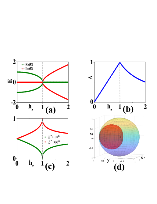
At $h_{x}=h_{z}$, a typical spontaneous $\mathcal{PT}$-symmetry breaking occurs: for the case of $h_{x}>h_{z},$ the energy levels $\left|+\right\rangle$ and $\left|-\right\rangle$ are $E_{\pm}=\pm\sqrt{h_{x}^{2}-h_{z}^{2}};$ For the case $h_{x}<h_{z},$ these two energy levels are $E_{\pm}=\pm i\sqrt{h_{z}^{2}-h_{x}^{2}};$ For the case of $h_{x}=h_{z}$, the system is at an EP with eigenstate coalescence and energy degeneracy. To strictly characterize the coalescence of the eigenstates, we define their state similarity, $\Lambda=|\langle\tilde{\psi}_{+}^{\mathrm{R}}|\tilde{\psi}_{-}^{\mathrm{R}}\rangle|$, where $|\tilde{\psi}_{+}^{\mathrm{R}}\rangle$ and $|\tilde{\psi}_{-}^{\mathrm{R}}\rangle$ are eigenstates satisfying the self-normalization conditions $|\langle\tilde{\psi}_{+}^{\mathrm{R}}|\tilde{\psi}_{+}^{\mathrm{R}}\rangle|=1$ and $|\langle\tilde{\psi}_{-}^{\mathrm{R}}|\tilde{\psi}_{-}^{\mathrm{R}}\rangle|=1$. Fig. 1(a) and Fig. 1(b) show the two energy levels and the state similarity $\Lambda$, respectively. It is obvious that both $E_{+}=E_{-}$ and $\Lambda=1$ hold at the EP ($h_{x}=h_{z}$).

Figure 1: (Color online) Physical properties of the EP ($h_{x}=h_{z}$) for the non-Hermitian two-level model $\hat{H}_{\mathrm{NH}}=h_{x}\sigma_{x}+ih_{z}\sigma_{z}$. $h_{x}$ is set to unity. (a) The two energy levels, $E_{\pm}.$ At the EP ($h_{x}=h_{z}$), these two energy levels become degenerate; (b) The state similarity $\Lambda=|\langle\tilde{\psi}_{+}^{\mathrm{R}}|\tilde{\psi}_{-}^{\mathrm{R}}\rangle|$ for two eigenstates $|\tilde{\psi}_{+}^{\mathrm{R}}\rangle$ and $|\tilde{\psi}_{-}^{\mathrm{R}}\rangle$ satisfying the self-normalization conditions $|\langle\tilde{\psi}_{+}^{\mathrm{R}}|\tilde{\psi}_{+}^{\mathrm{R}}\rangle|=1$ and $|\langle\tilde{\psi}_{-}^{\mathrm{R}}|\tilde{\psi}_{-}^{\mathrm{R}}\rangle|=1$. At the EP ($h_{x}=h_{z}$), we have $\Lambda=1$; (c) The self-normalization of the matrix basis, $\frac{1}{\mathcal{N}}^{\mathrm{R}}\langle 1|1\rangle^{\mathrm{R}}$ and $\frac{1}{\mathcal{N}}^{\mathrm{R}}\langle 2|2\rangle^{\mathrm{R}}$, where $\mathcal{N}=^{\mathrm{R}}\langle 1|1\rangle^{\mathrm{R}}+^{\mathrm{R}}\langle 2|2\rangle^{\mathrm{R}}.$ At the EP ($h_{x}=h_{z}$), we have $\frac{1}{\mathcal{N}}^{\mathrm{R}}\langle 1|1\rangle^{\mathrm{R}}=1$ and $\frac{1}{\mathcal{N}}^{\mathrm{R}}\langle 2|2\rangle^{\mathrm{R}}=0$; (d) The Bloch peach for the quantum states $|\psi^{\mathrm{R}}\rangle=\cos\frac{\theta}{2}\left|1\right\rangle^{\mathrm{R}}+e^{i\phi}\sin\frac{\theta}{2}\left|2\right\rangle^{\mathrm{R}}$ at the EP ($h_{x}=h_{z}$). Here, we have ${}^{\mathrm{R}}\langle 1|2\rangle^{\mathrm{R}}=0$, ${}^{\mathrm{R}}\langle 1|1\rangle^{\mathrm{R}}=1$, and ${}^{\mathrm{R}}\langle 2|2\rangle^{\mathrm{R}}=e^{-2\beta^{M}}$.

II.2 Singular non-Hermitian similar transformation

Let us understand why eigenvectors coalesce at EPs.

By performing a non-Hermitian similarity transformation $\mathcal{\hat{S}}_{M}=e^{-\beta^{M}\sigma_{y}}$, we transform the original non-Hermitian Hamiltonian $\hat{H}_{\mathrm{NH}}$ into a Hermitian/anti-Hermitian one, $\hat{H}_{0}$ ($\hat{H}_{0}^{\dagger}=\hat{H}_{0}$ or $\hat{H}_{0}^{\dagger}=-\hat{H}_{0}$), i.e.,

$$\hat{H}_{\mathrm{NH}}\rightarrow\mathcal{\hat{S}}_{M}^{-1}\hat{H}_{\mathrm{NH}}\mathcal{\hat{S}}_{M}=\hat{H}_{0},$$ (2)

where $\beta^{M}=\left|\frac{1}{2}\ln\left|\frac{h_{x}+h_{z}}{h_{x}-h_{z}}\right|\right|$. The eigenvalue of $\hat{H}_{0}$ is the same as that of $\hat{H}_{\mathrm{NH}}.$ Under the non-Hermitian similarity transformation $\mathcal{\hat{S}}_{M}$, the basis of $\hat{H}_{\mathrm{NH}}$ is correspondingly changed, i.e.,

$$\{|\psi_{0}^{\mathrm{R}}\rangle\}\rightarrow\{|\psi^{\mathrm{R}}\rangle\}=\{\mathcal{\hat{S}}_{M}(\sigma_{y},\beta^{M})|\psi_{0}\rangle\}.$$ (3)

In the following, we refer to $\{|\psi^{\mathrm{R}}\rangle\}$ as the matrix basis. If we select the initial basis $\{|\psi_{0}^{\mathrm{R}}\rangle\}$ to be the eigenstates of $\sigma_{y},$, i.e.,

$$\{|\psi_{0}^{\mathrm{R}}\rangle\} =\{\left|1\right\rangle,\left|2\right\rangle\}$$

$$=\{\frac{1}{\sqrt{2}}(\left|\uparrow\right\rangle+i\left|\downarrow\right\rangle),\frac{1}{\sqrt{2}}(\left|\uparrow\right\rangle-i\left|\downarrow\right\rangle)\},$$ (4)

then the matrix basis $\{|\psi^{\mathrm{R}}\rangle\}$ becomes

$$\{|\psi^{\mathrm{R}}\rangle\}=\{e^{-\beta^{M}\sigma_{y}}|\psi_{0}\rangle\}=\{\left|1\right\rangle^{\mathrm{R}},\left|2\right\rangle^{\mathrm{R}}\},$$ (5)

where $\left|1\right\rangle^{\mathrm{R}}=\left|1\right\rangle$ and $\left|2\right\rangle^{\mathrm{R}}=e^{-\beta^{M}}\left|2\right\rangle$. The matrix basis $\{\left|1\right\rangle^{\mathrm{R}},\left|2\right\rangle^{\mathrm{R}}\}$ obeys the orthogonal condition ${}^{\mathrm{R}}\langle 1|2\rangle^{\mathrm{R}}=0$ but does not obey the normalization conditions, i.e., ${}^{\mathrm{R}}\langle 1|1\rangle^{\mathrm{R}}=1$ and ${}^{\mathrm{R}}\langle 2|2\rangle^{\mathrm{R}}=e^{-2\beta^{M}}$.

Approaching the EP, the non-Hermitian similarity transformation becomes singular, i.e.,

$$\mathcal{\hat{S}}_{M}(\sigma_{y},\beta^{M})=e^{-\beta^{M}\sigma_{y}}$$ (6)

with $\beta^{M}=\left|\frac{1}{2}\ln\left|\frac{h_{x}+h_{z}}{h_{x}-h_{z}}\right|\right|\rightarrow\infty$. As a result, the matrix basis becomes defective, i.e.,

$$\{|\psi^{\mathrm{R}}\rangle\} =\{\mathcal{\hat{S}}_{M}(\sigma_{y},\beta^{M}\rightarrow\infty)|\psi_{0}\rangle\}$$

$$=\{\left|1\right\rangle^{\mathrm{R}},\left|2\right\rangle^{\mathrm{R}}\}\rightarrow\{\left|1\right\rangle^{\mathrm{R}},0\}.$$ (7)

Here, the base $\left|2\right\rangle^{\mathrm{R}}$  disappears! To illustrate the defectiveness of the matrix basis, in Fig. 1(c), we plot $\frac{1}{\mathcal{N}}^{\mathrm{R}}\langle 1|1\rangle^{\mathrm{R}}$ and $\frac{1}{\mathcal{N}}^{\mathrm{R}}\langle 2|2\rangle^{\mathrm{R}}$, where $\mathcal{N}=^{\mathrm{R}}\langle 1|1\rangle^{\mathrm{R}}+^{\mathrm{R}}\langle 2|2\rangle^{\mathrm{R}}$ is a normalization factor. Near the EP, $\frac{1}{\mathcal{N}}^{\mathrm{R}}\langle 2|2\rangle^{\mathrm{R}}$ becomes zero (${}^{\mathrm{R}}\langle 2|2\rangle^{\mathrm{R}}\rightarrow 0$).

As a result, according to the defective matrix basis without $\left|2\right\rangle^{\mathrm{R}},$ the two eigenstates $|\tilde{\psi}_{+}^{\mathrm{R}}\rangle$ and $|\tilde{\psi}_{-}^{\mathrm{R}}\rangle$ must coalesce into $\left|1\right\rangle$, i.e.,

$$|\tilde{\psi}_{+}^{\mathrm{R}}\rangle =\frac{1}{\sqrt{1+e^{-2\beta^{M}}}}(\left|1\right\rangle^{\mathrm{R}}+\left|2\right\rangle^{\mathrm{R}})$$

$$\rightarrow\frac{1}{\sqrt{1+e^{-2\beta^{M}}}}\left|1\right\rangle$$ (8)

and

$$|\tilde{\psi}_{-}^{\mathrm{R}}\rangle =\frac{1}{\sqrt{1+e^{-2\beta^{M}}}}(\left|1\right\rangle^{\mathrm{R}}-\left|2\right\rangle^{\mathrm{R}})$$

$$\rightarrow\frac{1}{\sqrt{1+e^{-2\beta^{M}}}}\left|1\right\rangle.$$ (9)

Now, near the EP, where $\beta^{M}\rightarrow\infty$, the state similarity $\Lambda=|\langle\tilde{\psi}_{+}^{\mathrm{R}}|\tilde{\psi}_{-}^{\mathrm{R}}\rangle|=\frac{1}{1+e^{-2\beta^{M}}}$ obviously approaches $1$. Thus, one can see that the singularity of the EP arises from the defective matrix basis $\{\left|1\right\rangle^{\mathrm{R}},0\}$ due to the singular non-Hermitian similarity transformation $\mathcal{\hat{S}}_{M}(\sigma_{y},\beta^{M}\rightarrow\infty)$.

II.3 Bloch peach for two-level states under the non-Hermitian similarity transformation

To further illustrate the singularity of EPs, we use a geometric approach to illustrate the deformation of the Bloch sphere under a singular non-Hermitian similarity transformation $\mathcal{\hat{S}}_{M}(\sigma_{y},\beta^{M}\rightarrow\infty)$.

For the Hermitian case, one may use a point on the Bloch sphere with SU(2) rotation symmetry to represent an arbitrary quantum state of the two-level system, i.e.,

$$|\psi\rangle=\cos\frac{\theta}{2}\left|1\right\rangle+e^{i\varphi}\sin\frac{\theta}{2}\left|2\right\rangle.$$ (10)

Here, $\theta\in[0,\pi]$ and $\varphi\in[0,2\pi]$ are real numbers, and the radius $r$ of the Bloch sphere can be obtained as $r=\langle\psi|\psi\rangle=1$.

For a two-level $\mathcal{PT}$ system, a quantum state under the non-Hermitian similarity transformation $\mathcal{\hat{S}}_{M}(\sigma_{y},\beta^{M})$ becomes

$$|\psi^{\mathrm{R}}\rangle=\mathcal{\hat{S}}_{M}|\psi\rangle=\cos\frac{\theta}{2}\left|1\right\rangle+e^{i\varphi}e^{-\beta^{M}}\sin\frac{\theta}{2}\left|2\right\rangle$$ (11)

(with $\theta\in[0,\pi]$ and $\varphi\in[0,2\pi]$), and the radius $R$ of the Bloch sphere can be obtained as

$$R=\langle\psi^{\mathrm{R}}|\psi^{\mathrm{R}}\rangle=\cos^{2}\frac{\theta}{2}+e^{-2\beta^{M}}\sin^{2}\frac{\theta}{2}.$$ (12)

Therefore, the original Bloch sphere changes into a peach-like closed surface with residue U(1) symmetry along the y-axis (we call this the Bloch peach). With increasing $\beta$, one pole of the Bloch peach moves upward. At the EP, this pole touches the origin of the coordinate system. See the illustration of the Bloch peach in the limit of $\beta^{M}\rightarrow\infty$ in Fig. 1(d).

III Protected non-Hermitian sub-systems

Before giving the definition of new type of EPs, we define protected non-Hermitian sub-systems.

Due to special conditions of symmetry/topology, there may exist protected sub-systems. To completely characterize the many-body model and its protected sub-systems, we give their definitions, $\{\hat{H}_{\mathrm{MB}},$ $B_{\mathrm{MB}}\}$ and $\{\hat{H}_{\mathrm{S}},$ $B_{\mathrm{S}}\},$ respectively. Here, both $\hat{H}_{\mathrm{MB}}$ and $\hat{H}_{\mathrm{S}}$ are Hermitian Hamiltonians, and both $B_{\mathrm{MB}}=\{|\Psi_{j}\rangle,j=1,2,...,N\}$ and $B_{\mathrm{S}}=\{\mathcal{P}|\Psi_{j}\rangle,j=1,2,...,N\}=\{|\mathrm{S}_{j}\rangle,j=1,2,...,K\}$ are normal basis with $B_{\mathrm{S}}=\mathcal{P}B_{\mathrm{MB}}\in B_{\mathrm{MB}}$ where $\mathcal{P}$ is a projected operator on the basis of the many-body system. It is obvious that $K<N$.

When one adds a non-Hermitian perturbation $i\delta\hat{H}$ on the many-body model, the total Hamiltonian becomes non-Hermitian, i.e.,

$$\hat{H}_{\mathrm{MB}}\rightarrow\hat{H}_{\mathrm{NH-MB}}=\hat{H}_{\mathrm{MB}}+i\delta\hat{H}.$$ (13)

Because the basis has no changing, the many-body model is denoted by $\{\hat{H}_{\mathrm{NH-MB}},$ $B_{\mathrm{MB}}\}$. In general, for a non-Hermitian sub-system, the biorthogonal set for the basis is defined by $|\Psi_{j}^{\mathrm{R}}\rangle$ and $|\Psi_{j}^{\mathrm{L}}\rangle$ ($j=1,2,...,K$), i.e.,

$$\hat{H}_{\mathrm{NH-MB}}|\Psi_{j}^{\mathrm{R}}\rangle=E_{j}|\Psi_{j}^{\mathrm{R}}\rangle,$$ (14)

and

$$\hat{H}_{\mathrm{NH-MB}}^{\dagger}|\Psi_{j}^{\mathrm{L}}\rangle=(E_{j})^{\ast}|\Psi_{j}^{\mathrm{L}}\rangle,$$ (15)

and $\langle\Psi_{j}^{\mathrm{L}}|\Psi_{j}^{\mathrm{R}}\rangle=1$ where $j$ is state index.

We then assume the non-Hermitian terms are perturbation and don’t change the existence of the protected sub-system and use $\{\hat{H}_{\mathrm{NH-S}},B_{\mathrm{S}}\}=\{\mathcal{P}\hat{H}_{\mathrm{MB}}\mathcal{P}^{-1},\mathcal{P}B_{\mathrm{MB}}\}$ to describe the protected (non-Hermitian) sub-system. Here, $\hat{H}_{\mathrm{NH-S}}=\mathcal{P}\hat{H}_{\mathrm{MB}}\mathcal{P}^{-1}$ is the effective Hamiltonian of the protected sub-system. Under the projected operation $\mathcal{P},$ the basis of the protected sub-system is obtained as

$$B_{\mathrm{MB}} =\{|\Psi_{j}^{\mathrm{R}}\rangle\}$$ (16)

$$\rightarrow B_{\mathrm{S}}=\mathcal{P}B_{\mathrm{MB}}=\{\mathcal{P}|\Psi_{j}^{\mathrm{R}}\rangle\}=\{|\psi_{j}^{\mathrm{R}}\rangle\}.$$

In addition, we show the method to calculate $\mathcal{\hat{H}}_{\mathrm{NH}}.$ Based on the basis $S_{\mathrm{NH}}=\{|\psi_{j}^{\mathrm{R}}\rangle\}$, an effective Hamiltonian of protected sub-system is derived as

$$\hat{H}_{\mathrm{NH-S}}={\displaystyle\sum\limits_{ij}}h_{IJ}$$ (17)

where

$$h_{IJ}=\left\langle\psi_{j}^{\mathrm{L}}\right|\hat{H}_{\mathrm{NH}}\left|\psi_{j}^{\mathrm{R}}\right\rangle,\text{ }I,J=1,2,...,K.$$ (18)

In particular, the basis of protected sub-sysrem $B_{\mathrm{S}}=\{|\psi_{j}^{\mathrm{R}}\rangle\}$ is always abnormal. For example, it does’t follow usual normalization $\langle\psi_{j}^{\mathrm{R}}|\psi_{j}^{\mathrm{R}}\rangle\neq 1$. In this paper, we only focus on the case of $K=2$.

IV General EPs – universal feature and classification

We next develop a universal theory for an arbitrary non-Hermitian protected two-level sub-system with a singularity and introduce the concept of general EPs. This phenomenon always occurs in subsystems of certain non-Hermitian models, for example, the defective edge states of a non-Hermitian topological insulator, the defective degenerate ground states in non-Hermitian systems with spontaneous symmetry breaking, or the topologically protected degenerate ground states in intrinsic topological orders.

A general non-Hermitian protected two-level sub-system is described by $\{\hat{H}_{\mathrm{NH}},\{|\psi_{0}^{\mathrm{R}}\rangle\}\}$. The Hamiltonian is

$$\hat{H}_{\mathrm{NH}}=h_{0}+\vec{h}\cdot\vec{\sigma},$$ (19)

where $h_{0}$ is a complex number, $\vec{h}=(h^{x},$ $h^{y},$ $h^{z})$ is a complex vector and $\vec{\sigma}=(\hat{\sigma}_{x},\hat{\sigma}_{y},\hat{\sigma}_{z})$ is the vector of Pauli matrices. $\{|\psi_{0}^{\mathrm{R}}\rangle\}=\{\mathcal{\hat{S}}_{B}|\psi_{0}\rangle\}$ denotes the initial basis where $\mathcal{\hat{S}}_{B}=e^{-\beta^{B}\cdot\vec{\sigma}^{B}}$ is a non-Hermitian similarity transformation with a real positive $\beta^{B}$ and $|\psi_{0}\rangle$ is a normal basis consisting of eigenstates of $\vec{\sigma}^{B}$ (or $\vec{\sigma}^{B}|\psi_{0}\rangle=\pm|\psi_{0}\rangle$).

IV.1 Representation under matrix basis

To identify the universal feature of general EPs, we transform the original non-Hermitian Hamiltonian $\hat{H}_{\mathrm{NH}}$ into a Hermitian/anti-Hermitian one and derive its representation under matrix basis, $\{\hat{H}_{0},\{|\psi^{\mathrm{R}}\rangle\}\}$.

First, we transform the non-Hermitian Hamiltonian $\hat{H}_{\mathrm{NH}}=h_{0}+\vec{h}\cdot\vec{\sigma}$ into

$$\hat{H}_{\mathrm{NH}}=h_{0}+(\operatorname{Re}\vec{h})\vec{\sigma}_{\operatorname{Re}}+i(\operatorname{Im}\vec{h})\vec{\sigma}_{\operatorname{Im}},$$ (20)

where $\vec{\sigma}_{\operatorname{Re}}$ and $\vec{\sigma}_{\operatorname{Im}}$ ($\vec{\sigma}_{\operatorname{Re}}\cdot\vec{\sigma}_{\operatorname{Re}}=1$ and $\vec{\sigma}_{\operatorname{Im}}\cdot\vec{\sigma}_{\operatorname{Im}}=1$) are the Pauli matrices corresponding to the real and imaginary parts of $\vec{h}$, respectively.

Second, we divide $i(\operatorname{Im}\vec{h})\vec{\sigma}_{\operatorname{Im}}$ into two parts, $i(\operatorname{Im}\vec{h})^{A}\vec{\sigma}_{\operatorname{Im}}^{A}$ and $i(\operatorname{Im}\vec{h})^{C}\vec{\sigma}_{\operatorname{Im}}^{C}$, with $\left[\vec{\sigma}_{\operatorname{Im}}^{C},\vec{\sigma}_{\operatorname{Re}}\right]=0$ and $\{\vec{\sigma}_{\operatorname{Im}}^{A},\vec{\sigma}_{\operatorname{Re}}\}=0.$ Then, the non-Hermitian Hamiltonian becomes

$$\hat{H}_{\mathrm{NH}}=h_{0}+\vec{h}_{\operatorname{Re}}^{\prime}\cdot\vec{\sigma}_{\operatorname{Re}}+i\vec{h}_{\operatorname{Im}}^{\prime}\cdot\vec{\sigma}_{\operatorname{Im}}^{A},$$ (21)

where $\vec{h}_{\operatorname{Re}}^{\prime}=(\operatorname{Re}\vec{h})+i(\operatorname{Im}\vec{h})^{C}$ and $\vec{h}_{\operatorname{Im}}^{\prime}=(\operatorname{Im}\vec{h})^{A}$.

Thirdly, under a non-Hermitian similarity transformation $\mathcal{\hat{S}}_{M}(\vec{\sigma}^{M},\beta^{M})$, we transform the original NH Hamiltonian $\hat{H}_{\mathrm{NH}}$ into a Hermitian/anti-Hermitian one, i.e.,

$$\hat{H}_{\mathrm{NH}} \rightarrow\mathcal{\hat{S}}_{M}^{-1}(\vec{\sigma}^{M},\beta^{M})\hat{H}_{\mathrm{NH}}\mathcal{\hat{S}}_{M}(\vec{\sigma}^{M},\beta^{M})$$

$$=\hat{H}_{0}=h_{0}+\sqrt{\vec{h}^{2}}\vec{\sigma}_{\operatorname{Re}},$$ (22)

where

$$\mathcal{\hat{S}}_{M}(\vec{\sigma}^{M},\beta^{M})=e^{-\beta^{M}\cdot\vec{\sigma}^{M}}$$ (23)

with $\vec{\sigma}^{M}=\frac{1}{2i}[\vec{\sigma}_{\operatorname{Im}}^{A},\vec{\sigma}_{\operatorname{Re}}]$ and $\beta^{M}=\left|\frac{1}{2}\ln\frac{\left|\vec{h}_{\operatorname{Re}}^{\prime}+\vec{h}_{\operatorname{Im}}^{\prime}\right|}{\left|\vec{h}_{\operatorname{Re}}^{\prime}-\vec{h}_{\operatorname{Im}}^{\prime}\right|}\right|$. As a result, the eigenvalue of $\hat{H}_{0}$ is the same as that of $\hat{H}_{\mathrm{NH}}$, i.e.,

$$E_{\pm}=h_{0}\pm\sqrt{\vec{h}^{2}}.$$ (24)

For the case of $\vec{h}^{2}>0,$ $\hat{H}_{0}$ is a Hermitian Hamiltonian, $\hat{H}_{0}=\hat{H}_{0}^{\dagger}$, whose energy levels $E_{\pm}=h_{0}\pm\left|\vec{h}\right|$ are real; for the case of $\vec{h}^{2}<0,$ $\hat{H}_{0}$ is an anti-Hermitian Hamiltonian, $\hat{H}_{0}=-\hat{H}_{0}^{\dagger}$, whose energy levels $E_{\pm}=h_{0}\pm i\left|\vec{h}\right|$ are an imaginary pair.

Finally, one can see that under the non-Hermitian similarity transformation, the initial basis $\{|\psi_{0}^{\mathrm{R}}\rangle\}$ is correspondingly changed into the unique matrix basis $\{|\psi^{\mathrm{R}}\rangle\}$, i.e.,

$$\{|\psi_{0}^{\mathrm{R}}\rangle\} \rightarrow\{|\psi^{\mathrm{R}}\rangle\}=\{\left|1\right\rangle^{\mathrm{R}},\left|2\right\rangle^{\mathrm{R}}\}$$

$$=\{\mathcal{\hat{S}}_{M}(\vec{\sigma}^{B},\beta^{B})|\psi_{0}^{\mathrm{R}}\rangle\}$$ (25)

$$=\{\mathcal{\hat{S}}_{M}(\vec{\sigma}^{M},\beta^{M})\mathcal{\hat{S}}_{B}(\vec{\sigma}^{B},\beta^{B})|\psi_{0}\rangle\}.$$

In addition, to describe the same non-Hermitian two-level system, one can also use another representation based on the normal basis, $\{\hat{H}_{\mathrm{NH}}^{\beta^{B}},\{|\psi_{0}\rangle\}\}$, i.e.,

$$\hat{H}_{\mathrm{NH}}^{\beta^{B}}=\mathcal{\hat{S}}_{B}^{-1}\hat{H}_{\mathrm{NH}}\mathcal{\hat{S}}_{B}$$ (26)

and $\{|\psi_{0}\rangle\}=\{\mathcal{\hat{S}}_{B}^{-1}|\psi_{0}^{\mathrm{R}}\rangle\}$. To clearly show the relationship among the three representations for the Hamiltonians of the same non-Hermitian two-level system, $\{\hat{H}_{\mathrm{NH}},\{|\psi_{0}^{\mathrm{R}}\rangle\}\}$ under the initial basis, $\{\hat{H}_{0},\{|\psi^{R}\rangle\}\}\}$ under the matrix basis, and $\{\hat{H}_{\mathrm{NH}}^{\beta^{B}},\{|\psi_{0}\rangle\}\}$ under the normal basis, we plot Fig. 2. $\mathcal{\hat{S}}_{M}$, $\mathcal{\hat{S}}_{B}$, and $\mathcal{\hat{S}}_{M}\mathcal{\hat{S}}_{B}$ are different non-Hermitian similarity transformations relating these representations.

Figure 2: (Color online) Schematic diagram of the relationship among three equivalent representations for a two-level system: $\{\hat{H}_{\mathrm{NH}},\{|\psi_{0}^{\mathrm{R}}\rangle\}\}$, under the initial basis; $\{\hat{H}_{0},\{|\psi^{R}\rangle\}\}$, under the matrix basis; and $\{\hat{H}_{\mathrm{NH}}^{\beta^{B}},\{|\psi_{0}\rangle\}\}$, under the normal basis. Here, $\hat{H}_{\mathrm{NH}}$ is the original non-Hermitian Hamiltonian with initial basis $\{|\psi_{0}^{\mathrm{R}}\rangle\}$. $\{|\psi^{R}\rangle\}=\{\mathcal{\hat{S}}_{M}|\psi_{0}^{\mathrm{R}}\rangle\}=\{\mathcal{\hat{S}}_{M}\mathcal{\hat{S}}_{B}|\psi_{0}\rangle\}$ is a matrix basis that classifies different types of GEPs (M-GEPs, B-GEPs, and H-GEPs). $\hat{H}_{\mathrm{NH}}^{\beta^{B}}=\mathcal{\hat{S}}_{B}\hat{H}_{\mathrm{NH}}\mathcal{\hat{S}}_{B}^{-1}$ classifies the subclasses of B-GEPs.

IV.2 Definition of general EPs

We point out that the universal feature of arbitrary non-Hermitian two-level systems with singularities is defectiveness of the matrix basis $\{|\psi^{\mathrm{R}}\rangle\}$ as $\beta^{M}\rightarrow\infty$ and/or $\beta^{B}\rightarrow\infty$ rather than energy degeneracy or state coalescence. Thus, we define general EPs as follows:

Definition – general EPs (GEPs): For an arbitrary non-Hermitian two-level system, GEPs exist if and only if the matrix basis $\{|\psi^{\mathrm{R}}\rangle\}=\{\left|1\right\rangle^{\mathrm{R}},\left|2\right\rangle^{\mathrm{R}}\}$ becomes defective, i.e., $\frac{1}{\mathcal{N}}^{\mathrm{R}}\langle 1|1\rangle^{\mathrm{R}}=1$ and ${}^{\mathrm{R}}\langle 2|2\rangle^{\mathrm{R}}=0$ or $\frac{1}{\mathcal{N}}^{\mathrm{R}}\langle 2|2\rangle^{\mathrm{R}}=1$ and ${}^{\mathrm{R}}\langle 1|1\rangle^{\mathrm{R}}=0$. Here, $\mathcal{N}=^{\mathrm{R}}\langle 1|1\rangle^{\mathrm{R}}+^{\mathrm{R}}\langle 2|2\rangle^{\mathrm{R}}$ is a normalization factor.

As a result, at GEPs, the two energy levels may not necessarily be degenerate, i.e., $E_{+}=E_{-}$ and $E_{+}\neq E_{-}$ are both allowed; the two eigenstates $\left|\tilde{\psi}_{+}^{\mathrm{R}}\right\rangle$ and $\left|\tilde{\psi}_{-}^{\mathrm{R}}\right\rangle$ may not necessarily coalesce, i.e., $\Lambda\equiv 1$ and $\Lambda\equiv 0$ are both allowed. In addition, in the form of Jordan block matrix, at GEPs the algebra multiplier of a matrix may be same to its geometric multiplier.

IV.3 Classification of general EPs

By considering different behaviors of defective bases, we can classify GEPs for an arbitrary non-Hermitian two-level system. Depending on the behavior of the defective matrix basis $\{|\psi^{\mathrm{R}}\rangle\}=\{\mathcal{\hat{S}}_{M}(\vec{\sigma}^{M},\beta^{M})\mathcal{\hat{S}}_{B}(\vec{\sigma}^{B},\beta^{B})|\psi_{0}\rangle\},$ there are three types of GEPs: matrix-type GEPs (or M-GEPs), with $\beta^{M}\rightarrow\infty$ and $\beta^{B}\nrightarrow\infty$; basis-type GEPs (or B-GEPs), with $\beta^{M}\nrightarrow\infty$ and $\beta^{B}\rightarrow\infty$; and hybrid-type GEPs (or H-GEPs), with $\beta^{M}\rightarrow\infty$ and $\beta^{B}\rightarrow\infty$.

In addition, there are two different classes of B-GEPs, i.e., IB-GEPs and IIB-GEPs. For IB-GEPs, the two eigenstates will never coalesce with each other, i.e., $\Lambda\equiv 0$; for IIB-GEPs, the two eigenstates will always coalesce each other, i.e., $\Lambda\equiv 1$.

To show the physical properties of these two classes of B-GEPs, we perform a non-Hermitian similarity transformation $\mathcal{\hat{S}}_{B}^{-1}$ on the initial basis $\{|\psi_{0}^{\mathrm{R}}\rangle$ and obtain a representation under the normal basis, i.e.,

$$\{|\psi_{0}^{\mathrm{R}}\rangle\}\rightarrow\{\mathcal{\hat{S}}_{B}^{-1}|\psi_{0}^{\mathrm{R}}\rangle\}=\{|\psi_{0}\rangle\}.$$ (27)

Correspondingly, the original Hamiltonian $\hat{H}_{\mathrm{NH}}$ is transformed into

$$\hat{H}_{\mathrm{NH}}^{\beta^{B}}=\mathcal{\hat{S}}_{B}\hat{H}_{\mathrm{NH}}\mathcal{\hat{S}}_{B}^{-1}.$$ (28)

There are two possibilities for $\hat{H}_{\mathrm{NH}}^{\beta^{B}}$, which correspond to the two classes of B-GEPs: one possibility is that all elements of $\hat{H}_{\mathrm{NH}}^{\beta^{B}}$ are finite, in which case the eigenstates do not coalesce (or $\Lambda\equiv 0$), and the other is one or more elements diverge, i.e., $(\hat{H}_{\mathrm{NH}}^{\beta^{B}})_{ij}\rightarrow\infty$, in which case the eigenstates coalesce (or $\Lambda\equiv 1$). It is obvious that at IB-GEPs the algebra multiplier of the Hamiltonian $\hat{H}_{\mathrm{NH}}$ is equal to its geometric multiplier.

Therefore, there exists a quantum phase transition between IB-GEPs (the region without eigenstate coalescence) and IIB-GEPs (the region with eigenstate coalescence). Let us give a simple explanation of this fact.

For IB-GEPs, the Hamiltonian $\hat{H}_{\mathrm{NH}}$ commutes with $\vec{\sigma}^{B}$, i.e., $[\hat{H}_{\mathrm{NH}},\vec{\sigma}^{B}]=0$. As a result, the Hamiltonian $\hat{H}_{\mathrm{NH}}$ must be written as $\lambda\vec{\sigma}^{B}$ with $\lambda\neq 0$. Under the non-Hermitian similarity transformation $\mathcal{\hat{S}}_{B}^{-1}=e^{\beta^{B}\vec{\sigma}^{B}}$, we have

$$\hat{H}_{\mathrm{NH}}^{\beta^{B}}=\mathcal{\hat{S}}_{B}^{-1}\hat{H}_{\mathrm{NH}}\mathcal{\hat{S}}_{B}=\lambda\vec{\sigma}^{B}.$$ (29)

Now, the matrix basis becomes normal, i.e.,

$$\{|\psi_{0}^{\mathrm{R}}\rangle\}\rightarrow\{\mathcal{\hat{S}}_{B}^{-1}|\psi_{0}^{\mathrm{R}}\rangle\}=\{|\psi_{0}\rangle\}.$$ (30)

Here, the $|\psi_{0}\rangle$ are eigenstates of $\vec{\sigma}^{B}$, or $\vec{\sigma}^{B}|\psi_{0}\rangle=\pm|\psi_{0}\rangle$. Because the eigenstates $|\psi_{\pm}^{\mathrm{R}}\rangle$ of $\hat{H}_{\mathrm{NH}}=\lambda\vec{\sigma}^{B}$ are also those of $|\psi_{0}\rangle$, the state similarity of $|\psi_{\pm}^{\mathrm{R}}\rangle$ must be zero, i.e.,

$$\Lambda=|\langle\tilde{\psi}_{+}^{\mathrm{R}}|\tilde{\psi}_{-}^{\mathrm{R}}\rangle|=0.$$ (31)

On the other hand, for IIB-GEPs, the Hamiltonian $\hat{H}_{\mathrm{NH}}$ does not commute with $\vec{\sigma}^{B},$ i.e., $[\hat{H}_{\mathrm{NH}},\vec{\sigma}^{B}]\neq 0$. The Hamiltonian $\hat{H}_{\mathrm{NH}}$ must be written as

$$\hat{H}_{\mathrm{NH}}=\lambda\vec{\sigma}^{B}+\eta(\vec{\sigma}^{B})^{\perp}$$ (32)

with $\lambda^{2}+\eta^{2}\neq 0$ and $\{(\vec{\sigma}^{B})^{\perp},\vec{\sigma}^{B}\}=0$. Now, one element of $\hat{H}_{\mathrm{NH}}^{\beta^{B}}=\mathcal{\hat{S}}_{B}^{-1}\hat{H}_{\mathrm{NH}}\mathcal{\hat{S}}_{B}$ diverges. On the basis of $\{|\psi_{0}\rangle\}$, the divergent term is proportional to $(\begin{array}[c]{cc}0&1\\ 0&0\end{array})$ or $(\begin{array}[c]{cc}0&0\\ 1&0\end{array})$. As a result, the Hamiltonian $\hat{H}_{\mathrm{NH}}^{\beta^{B}}=\mathcal{\hat{S}}_{B}^{-1}\hat{H}_{\mathrm{NH}}\mathcal{\hat{S}}_{B}$ is dominated by this divergent term, and we can ignore other terms. In this case, the state similarity of $|\psi_{\pm}^{\mathrm{R}}\rangle$ must be $1$, i.e.,

$$\Lambda=|\langle\tilde{\psi}_{+}^{\mathrm{R}}|\tilde{\psi}_{-}^{\mathrm{R}}\rangle|=1.$$ (33)

Without sudden changing the energy levels and the defectiveness of matrix basis, this quantum phase transition is always “hidden”.

V Example: 1D nonreciprocal Su–Schrieffer–Heeger model

V.1 The model

In this section, we take the 1D nonreciprocal Su–Schrieffer–Heeger (SSH) model as an example to illustrate the different types of GEPs for its topologically protected sub-space of two edge states.

The Bloch Hamiltonian for the nonreciprocal SSH model under periodic boundary conditions (PBC) is given by

$$\hat{H}_{\mathrm{PBC}}(k) =\sum_{k}c_{k}^{\dagger}\tau_{x}\left(t_{1}+t_{2}\cos k\right)c_{k}$$ (34)

$$+\sum_{k}c_{k}^{\dagger}\tau_{y}\left(t_{2}\sin k+i\gamma\right)c_{k}+i\varepsilon\sum_{k}c_{k}^{\dagger}\tau_{z}c_{k},$$

where $c_{k}^{\dagger}=(c_{k,\mathrm{A}}^{\dagger},c_{k,\mathrm{B}}^{\dagger})$; the $\tau_{i}$ are the Pauli matrices acting on the (A or B) sublattice subspaces; $t_{1}$ and $t_{2}$ describe the intracell and intercell hopping strengths, respectively; $\gamma$ describes unequal intracell hopping; and $\varepsilon$ denotes the strength of an imaginary staggered potential on the two sublattices. $t_{1}$, $t_{2}$, $\gamma$, and $\varepsilon$ are all real. In this paper, we set $t_{2}=1$.

Under a non-Hermitian similarity transformation $\mathcal{\hat{S}}_{\mathrm{NHP}}$, the physics properties of the 1D nonreciprocal SSH model under open boundary conditions (OBC) are characterized by $\hat{H}_{\mathrm{OBC}}(k)$ rather than $\hat{H}_{\mathrm{PBC}}(k)$Yao . Here, the non-Hermitian similarity transformation $\mathcal{\hat{S}}_{\mathrm{NHP}}$ given by

$$c_{k}^{\dagger}\rightarrow\tilde{c}_{k}^{\dagger}=c_{k-iq_{0}}^{\dagger}=\mathcal{\hat{S}}_{\mathrm{NHP}}c_{k}^{\dagger}$$ (35)

or

$$c_{n}^{\dagger}\rightarrow\tilde{c}_{n}^{\dagger}=e^{-q_{0}(n-1)}c_{n}^{\dagger}=\mathcal{\hat{S}}_{\mathrm{NHP}}c_{n}^{\dagger}$$ (36)

where $e^{q_{0}}=\sqrt{\frac{t_{1}-\gamma}{t_{1}+\gamma}}.$ Consequently, the effective hopping parameters become $\bar{t_{1}}=\sqrt{(t_{1}+\gamma)(t_{1}-\gamma)}$ and $\bar{t_{2}}=t_{2}$.

To characterize the topological properties of the non-Hermitian topological system, the non-Bloch topological invariant $\bar{w}$ of $\hat{H}_{\mathrm{OBC}}(k)$ is introduced, i.e.,

$$\bar{w}=\frac{1}{2\pi}\int_{-\pi}^{\pi}\partial\bar{\phi}(k)dk$$ (37)

where $\bar{\phi}(k)=\tan^{-1}(\bar{h}_{y}/\bar{h}_{x})$ and $\bar{h}_{x}=\bar{t}_{1}+\bar{t}_{2}\cos k$, $\bar{h}_{y}=\bar{t}_{2}\sin k$. In the region of $\left|\bar{t}_{1}\right|<\left|\bar{t}_{2}\right|$ and $\bar{w}=1$, the system is a topological insulator (the gray region in Fig. 3(a)); in the region of $\left|\bar{t}_{1}\right|>\left|\bar{t}_{2}\right|$ and $\bar{w}=0$, the system is a normal insulator (the white region in Fig. 3(a)). A quantum phase transition occurs at $\left|\bar{t}_{1}\right|=\left|\bar{t}_{2}\right|$, where the bulk energy gap under OBC is closed.

V.2 Two-level systems from two edge states in topological phase

In the topological phase with $\bar{w}=1$, there exist two edge states $\left|\psi_{1}^{\mathrm{R}}\right\rangle$ and $\left|\psi_{2}^{\mathrm{R}}\right\rangle$. These two edge states make up a topologically protected subspace denoted by $\{\hat{H}_{\mathrm{NH}},\{|\psi_{0}^{\mathrm{R}}\rangle\}\}$. Under the biorthogonal set, the initial basis $\{|\psi_{0}^{\mathrm{R}}\rangle\}$ is $\{\left|\psi_{1}^{\mathrm{R}}\right\rangle,\ \left|\psi_{2}^{\mathrm{R}}\right\rangle\}$. The effective Hamiltonian $\hat{H}_{\mathrm{NH}}$ is written as

$$\hat{H}_{\mathrm{NH}}=\left(\begin{array}[c]{cc}h_{11}&h_{12}\\ h_{21}&h_{22}\end{array}\right),$$ (38)

where $h_{ij}=\left\langle\psi_{i}^{\mathrm{L}}\right|\hat{H}\left|\psi_{j}^{\mathrm{R}}\right\rangle$, $i,j=1,2$. Through straightforward calculationsRan , we can analytically obtain the effective Hamiltonian of the two edge states as

$$\hat{H}_{\mathrm{NH}}=\bar{\Delta}\sigma^{x}+i\varepsilon\sigma^{z},$$ (39)

where $\bar{\Delta}=\frac{(\bar{t}_{2}^{2}-\bar{t}_{1}^{2})}{\bar{t}_{2}}(\frac{\bar{t}_{1}}{\bar{t}_{2}})^{N}$. The two energy levels for the two eigenstates $|\psi_{+}^{\mathrm{R}}\rangle$ and $|\psi_{-}^{\mathrm{R}}\rangle$ are $E=\pm\sqrt{\bar{\Delta}^{2}-\varepsilon^{2}}$.

Figure 3: (Color online) (a) is the global phase diagram for the 1D nonreciprocal SSH model under open boundary conditions ($N=20$ and $\varepsilon=0.001$): four red dots $\rightarrow$ M-GEPs; solid black lines $\rightarrow$ H-GEPs; yellow region $\rightarrow$ IB-GEPs; gray region $\rightarrow$ IIB-GEPs; dashed lines $\rightarrow$ hidden quantum phase transition between IB-GEPs and IIB-GEPs. (b₁), (b₂) and (b₃) show examples of the Bloch peaches for M-GEPs, B-GEPs, and H-GEPs, respectively.

V.3 General EPs

Then, based on $\{\hat{H}_{\mathrm{NH}},\{|\psi_{0}^{\mathrm{R}}\rangle\}\}$, we study the GEPs for the two edge states in the 1D nonreciprocal SSH model.

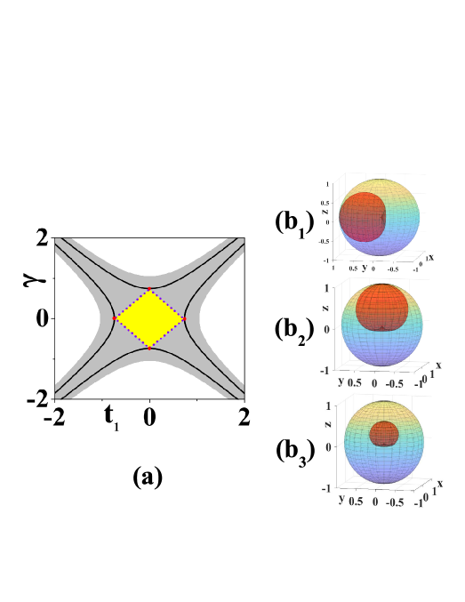
In topological phase with $\bar{w}=1$ (or $\left|\bar{t}_{1}\right|<\left|\bar{t}_{2}\right|$), we have GEPs for the two edge states except for the Hermitian/anti-Hermitian cases at $\gamma=0$ or $t_{1}=0$. Fig. 3(a) is an illustration of the global phase diagram for GEPs: the four red dots correspond to M-GEPs, the solid black lines correspond to H-GEPs, the yellow region corresponds to IB-GEPs, and the gray region corresponds to IIB-GEPs. The Bloch peaches for different types of GEPs are illustrated in Fig. 3(b₁) (an example for M-GEPs), Fig. 3(b₂) (an example for B-GEPs), and Fig. 3(b₃) (an example for H-GEPs).

Let us separately discuss the different types of GEPs one-by-one.

Figure 4: (Color online) (a) is the energy levels of two edge states; (b) is the state similarity of two edge states, $\Lambda=|\langle\tilde{\psi}_{+}^{\mathrm{R}}|\tilde{\psi}_{-}^{\mathrm{R}}\rangle|$. (a) and (b) are all for the case of $N=50$ , $t_{2}=1$, $\varepsilon=0.001$ and $t_{1}=0$. The two energy levels become degenerate and the state similarity becomes $1$ at the gray dotted line ($\gamma=\pm 0.86$), where the M-GEP occurs.

V.3.1 M-GEPs

Firstly, we consider the case of M-GEPs by setting $\varepsilon$ to a purely real value and $\gamma=0$. Now, the initial basis becomes normal, i.e.,

$$\{|\psi_{0}^{\mathrm{R}}\rangle\}=\{|\psi_{0}\rangle\}$$ (40)

with $\mathcal{\hat{S}}_{B}(\vec{\sigma}^{B},\beta^{B})=1$. The Hamiltonian of the effective two-level model is reduced to

$$\hat{H}_{\mathrm{NH}}=i\varepsilon\sigma^{z}+\Delta_{0}\sigma^{x},$$ (41)

where $\Delta_{0}=\frac{\left(t_{2}^{2}-t_{1}^{2}\right)}{t_{2}}(-\frac{t_{1}}{t_{2}})^{N}$.

A spontaneous $\mathcal{PT}$-symmetry-breaking transition occurs at $\left|\varepsilon\right|=\Delta_{0}.$ The energy levels become degenerate, shown as Fig. 4(a) i.e.,

$$E_{\pm}=\pm\sqrt{\varepsilon^{2}-\Delta_{0}^{2}}\rightarrow 0,$$ (42)

and the non-Hermitian similarity transformation becomes singular, i.e.,

$$\mathcal{\hat{S}}_{M}=e^{-\beta^{M}\cdot\sigma^{y}}$$ (43)

with $\beta^{M}=\left|\frac{1}{2}\ln\left|\frac{\Delta_{0}+\varepsilon}{\Delta_{0}-\varepsilon}\right|\right|\rightarrow\infty.$ We have an M-GEP with the following defective matrix basis:

$$\{|\psi^{\mathrm{R}}\rangle\}=\{\mathcal{\hat{S}}_{M}(\sigma^{y},\beta^{M}\rightarrow\infty)|\psi_{0}\rangle\}.$$ (44)

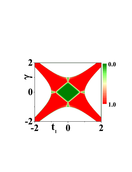
The state similarity $\Lambda=|\langle\tilde{\psi}_{+}^{\mathrm{R}}|\tilde{\psi}_{-}^{\mathrm{R}}\rangle|=1$ indicates the coalescence of the two edge states, shown as the Fig. 4(b). From the illustration of Fig. 4, we can obtain that at M-GEPs two energy levels become degenerate and two energy states coalesce ($E_{+}\neq E_{-}$, $\Lambda=1$), shown as the gray dotted line at $\gamma=\pm 0.86$. In addition, as shown in Fig. 3(b₁), the Bloch peach has a symmetric axis along the y-direction.

Figure 5: (Color online) (a) is the energy levels of two edge states; (b) is the state similarity of two edge states, $\Lambda=|\langle\tilde{\psi}_{+}^{\mathrm{R}}|\tilde{\psi}_{-}^{\mathrm{R}}\rangle|$. (a) and (b) are all for the case of $N=50$, $t_{2}=1$, $\varepsilon=0.001$ and $\gamma=0.5$. The two energy levels become degenerate ($E_{+}=E_{-}$) at the gray dotted line ($t_{1}=1.03$), where the H-GEP occurs with $\Lambda=1$; The orange dotted line ($t_{1}=0.38$) denoted the phase transition between IB-GEPs ($E_{+}\neq E_{-}$, $\Lambda=0$) and IIB-GEPs ($E_{+}\neq E_{-}$, $\Lambda=1$).

V.3.2 B-GEPs

Secondly, we consider the case of B-GEPs by setting $\left|\bar{\Delta}\right|\neq\left|\varepsilon\right|$ with $t_{1}\neq 0$ and $\gamma\neq 0$. Now, the initial basis becomes defective, i.e.,

$$\{|\psi_{0}^{\mathrm{R}}\rangle\}=\{\mathcal{\hat{S}}_{B}|\psi_{0}\rangle\}$$

with $\mathcal{\hat{S}}_{B}=e^{-\beta^{B}\cdot\sigma_{z}}$ and $\beta^{B}=Nq_{0}.$ Here, $q_{0}=\frac{1}{2}\ln(\frac{t_{1}-\gamma}{t_{1}+\gamma})$ is an imaginary wave vector that characterizes the non-Hermitian skin effect. In the thermodynamic limit $N\rightarrow\infty$, we have a B-GEP with the following defective matrix basis:

$$\{|\psi^{\mathrm{R}}\rangle\}=\{|\psi_{0}^{\mathrm{R}}\rangle\}=\{\mathcal{\hat{S}}_{B}(\sigma^{z},\beta^{B}\rightarrow\infty)|\psi_{0}\rangle\}.$$ (45)

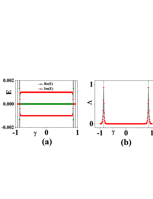
In Fig. 3(a), except for the black lines and red dots, B-GEPs exist throughout the whole topological insulator region. An interesting fact is that the energy levels are not degenerate, shown as Fig. 5(a), i.e.,

$$E_{\pm}=\pm\sqrt{\bar{\Delta}^{2}-\varepsilon^{2}}\neq 0.$$ (46)

As a result, this is an example of GEPs without energy degeneracy. Now, the Bloch peach has a symmetric axis along the z-direction; see the illustration in Fig. 3(b₂).

Let us discuss the classes of B-GEPs in detail.

After the application of a non-Hermitian similarity transformation $\mathcal{\hat{S}}_{B}$, the effective two-level model $\hat{H}_{\mathrm{NH}}$ is transformed into another non-Hermitian model, i.e.,

$$\hat{H}_{\mathrm{NH}}^{\beta^{B}} =(\mathcal{\hat{S}}_{B})^{-1}\hat{H}_{\mathrm{NH}}(\mathcal{\hat{S}}_{B})$$

$$=\bar{\Delta}^{+}\sigma^{+}+\bar{\Delta}^{-}\sigma^{-}+i\varepsilon\sigma^{z},$$ (47)

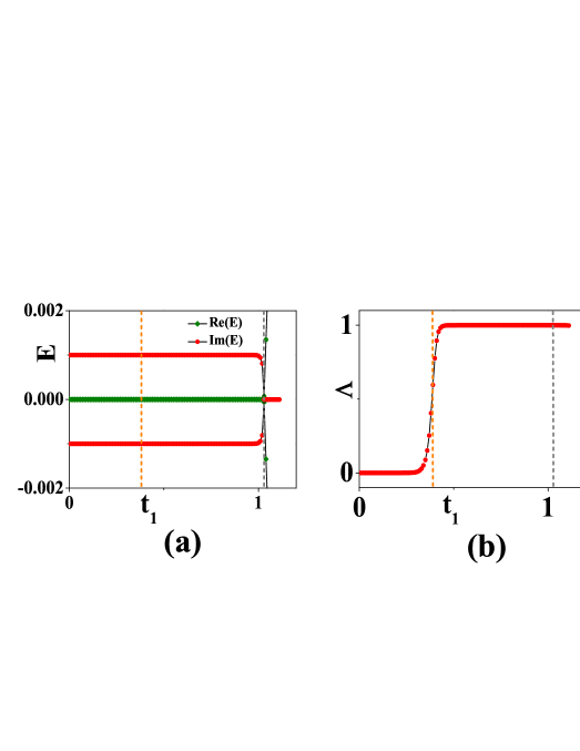
where $\bar{\Delta}^{+}=\bar{\Delta}\exp{(-Nq_{0})}$ and $\bar{\Delta}^{-}=\bar{\Delta}\exp{(Nq_{0})}$. In the thermodynamic limit $N\rightarrow\infty$, there exist three phases: a phase with $\left|\bar{\Delta}^{+}\right|\rightarrow\infty$ and $\left|\bar{\Delta}^{-}\right|\rightarrow 0$, a phase with $\left|\bar{\Delta}^{+}\right|\rightarrow 0$ and $\left|\bar{\Delta}^{-}\right|\rightarrow\infty$, and a phase with $\left|\bar{\Delta}^{+}\right|\rightarrow 0$ and $\left|\bar{\Delta}^{-}\right|\rightarrow 0$. At $\left|\bar{\Delta}^{\pm}\right|=1$ or $t_{1}\pm\gamma=\pm 1$, the “hidden” quantum phase transition occurs, with a sudden change between IB-GEPs ($\Lambda=0$) and IIB-GEPs ($\Lambda=1$). Shown as Fig. 5, the orange dotted line at $t_{1}=0.38$ identifies the phase transition between IB-GEPs ($E_{+}\neq E_{-}$, $\Lambda=0$) and IIB-GEPs ($E_{+}\neq E_{-}$, $\Lambda=1$). We find that the situation changes for the state similarity $\Lambda=|\langle\tilde{\psi}_{+}^{\mathrm{R}}|\tilde{\psi}_{-}^{\mathrm{R}}\rangle|$ of two edge states. In Fig. 6, one can see the “hidden” quantum phase transition from the numerical results for the case of $N=20$ and $\varepsilon=0.001$ that $\Lambda$ suddenly changes from $0$ to $1$ at $\left|\bar{\Delta}^{\pm}\right|=1.$

Figure 6: (Color online) The state similarity of two edge states, $\Lambda=|\langle\tilde{\psi}_{+}^{\mathrm{R}}|\tilde{\psi}_{-}^{\mathrm{R}}\rangle|$, for the case of $N=20$ and $\varepsilon=0.001$ as a function of $\gamma$ and $t_{1}$. A hidden phase transition occurs with a sudden change between IB-GEPs ($\Lambda=0$, green regions) and IIB-GEPs ($\Lambda=1$, red regions).

V.3.3 H-GEPs

Thirdly, we consider the case of H-GEPs by setting $\varepsilon$ to a purely real value, $\gamma\neq 0,$ and $\left|\bar{\Delta}\right|=\left|\varepsilon\right|$. On the one hand, the initial basis is defective, i.e.,

$$\{|\psi_{0}^{\mathrm{R}}\rangle\}=\{\mathcal{\hat{S}}_{B}|\psi_{0}\rangle\}=\{e^{-\beta^{B}\cdot\sigma_{z}}|\psi_{0}\rangle\}$$ (48)

with $\beta^{B}=Nq_{0}\rightarrow\infty$. In the thermodynamic limit $N\rightarrow\infty$, the two-level system may be regarded as a B-GEP. On the other hand, for the case of $\left|\frac{\bar{\Delta}}{\varepsilon}\right|=1$, the same system can be regarded as an M-GEP with another singular non-Hermitian similarity transformation $\mathcal{\hat{S}}_{B}(\beta^{M}\rightarrow\infty)$.

Therefore, in thermodynamic limit $N\rightarrow\infty$, we have an H-GEP with the following defective matrix basis:

$$\{|\psi^{\mathrm{R}}\rangle\} =\{\mathcal{\hat{S}}_{M}(\sigma_{y},\beta^{M}=\left|\frac{1}{2}\ln\left|\frac{\bar{\Delta}+\varepsilon}{\bar{\Delta}-\varepsilon}\right|\right|\rightarrow\infty)$$

$$\cdot\mathcal{\hat{S}}_{B}(\sigma_{z},\beta^{B} =Nq_{0}\rightarrow\infty)|\psi_{0}\rangle\}.$$

Now, the quantum state under the non-Hermitian similarity transformations $\mathcal{\hat{S}}_{M}(\sigma_{y},\beta^{M})$ and $\mathcal{\hat{S}}_{B}(\sigma_{z},\beta^{B})$ becomes

$$|\psi^{\mathrm{R}}\rangle =\frac{1}{\sqrt{2}}(\cos\frac{\theta}{2}+e^{-\beta^{B}}\sin\frac{\theta}{2})\left|1\right\rangle$$ (49)

$$+\frac{i}{\sqrt{2}}e^{i\varphi}e^{-\beta^{M}}(\cos\frac{\theta}{2}-e^{-\beta^{B}}\sin\frac{\theta}{2})\left|2\right\rangle$$

(with $\theta\in[0,\pi]$ and $\varphi\in[0,2\pi]$), and the radius of the Bloch sphere $R$ can be obtained as

$$R =\langle\psi^{\mathrm{R}}|\psi^{\mathrm{R}}\rangle=\frac{1}{\sqrt{2}}[(\cos\frac{\theta}{2}+e^{-\beta^{B}}\sin\frac{\theta}{2})^{2}$$ (50)

$$+e^{-2\beta^{M}}(\cos\frac{\theta}{2}-e^{-\beta^{B}}\sin\frac{\theta}{2})^{2}]^{1/2}.$$

As shown in Fig. 3(b₃), the Bloch peach, with a symmetric axis along the z-direction, shrinks.

In addition, for the non-Hermitian SSH model, the H-GEP is an unusual spontaneous $\mathcal{PT}$-symmetry breaking accompanied by a transition from real to complex spectra. From Fig. 6, the two energy levels become degenerate ($E_{+}=E_{-}$) at the gray dotted line with $t_{1}=1.03$, where the H-GEP occurs, and we can see that the state similarity of the two edge states is constant, i.e., $\Lambda\equiv 1$.

VI Conclusion and discussion

In this paper, we illustrate that the phenomenon of EPs in non-Hermitian quantum systems is much more interesting than expected. For general non-Hermitian two-level systems, there may exist three types of GEPs — M-GEPs (with a defective matrix basis and a normal initial basis), B-GEPs (with a normal matrix basis and a defective initial basis), and H-GEPs (with a defective matrix basis and a defective initial basis). In addition, there are two classes of B-GEPs — IB-GEPs, without eigenstate coalescence, and IIB-GEPs, with eigenstate coalescence. By taking the topologically protected edge states in the non-Hermitian SSH model as an example, we explore the physical properties of GEPs. In the future, we will study higher-order GEPs in non-Hermitian systems and attempt to develop a complete theory of GEPs.