did2s: Two-Stage Difference-in-Differences

Abstract

Recent work has highlighted the difficulties of estimating difference-in-differences models when the treatment is adopted at different times for different units. This article introduces the R package did2s which implements the estimator introduced in Gardner (2021). The article provides an approachable review of the underlying econometric theory and introduces the syntax for the function did2s. Further, the package introduces functions, event_study and plot_event_study, which uses a common syntax to implement all of the modern event-study estimators.

Introduction

A rapidly growing econometric literature has identified difficulties in traditional difference-in-differences estimation when treatment turns on at different times for different groups and when the effects of treatment vary across groups and over time (Callaway and Sant’Anna, 2020; Sun and Abraham, 2020; Goodman-Bacon, 2018; Borusyak et al., 2021; de Chaisemartin and D’Haultfoeuille, 2019). Gardner (2021) proposes an estimator of the two-way fixed-effects model that is quick and intuitive. The estimator relies on the standard two-way fixed-effect model (see the following section) and forms an intuitive estimate: the average difference in outcomes between treated and untreated units after removing fixed unit- and time-invariant shocks.

This article first discusses the modern difference-in-differences theory in an approachable way and second discusses the software package, did2s, which implements the two-stage estimation approach proposed by Gardner (2021) to estimate robustly the two-way fixed-effects (TWFE) model. There are two notable technical features of this package. First, did2s utilizes the incredibly fast package, fixest (Bergé, 2018), which can estimate regressions with a high number of fixed-effects very quickly. Since there are a few alternative TWFE event-study estimators implemented in R, each with their own syntax and data formatting requirements, the package also has a set of functions that allow quick estimation and plotting of every alternative event study estimator using a standardized syntax. This allows for easy comparison between the results of different methods.

Difference-in-Differences Theory

Researchers commonly use the difference-in-differences (DiD) methodology to estimate the effects of treatment in the case where treatment is non-randomly assigned. Instead of random assignment giving rise to identification, the DiD method relies on the so-called “parallel trends” assumption, which asserts that outcomes would evolve in parallel between the treated and untreated groups in a world where the treated were untreated. This is formalized with the two-way fixed-effects (TWFE) model. In a static setting where treatment effects are constant across treatment groups and over time, researchers estimate the static TWFE model:

$$y_{igt}=\mu_{g}+\eta_{t}+\tau D_{gt}+\varepsilon_{igt},$$ (1)

where $y_{igt}$ is the outcome variable of interest, $i$ denotes the individual, $t$ denotes time, and $g$ denotes group membership where “group” is defined as all units that start treatment at time $g$. $\mu_{g}$ is a vector of time-invariant group characteristics, $\eta_{t}$ is a vector of shocks in a given time period that is experienced by all individuals equally, and $D_{gt}$ is an indicator for whether initial-treatment group $g$ is receiving treatment in period $t$, i.e. $D_{gt}\equiv\mathbb{1}(g\leq t)$. The coefficient of interest is $\tau$, which is the (constant) average effect of the treatment on the treated (ATT). If it is indeed true that the treatment effect is constant across groups and over time, then the estimate formed by estimating the static TWFE model will be consistent for $\tau$.

However, treatment effects are not constant in most settings. The magnitude of a unit’s treatment effect can differ based on group status $g$ (e.g. if groups that benefit more from a policy implement it earlier) and treatment duration (e.g. if treatment effects grow as the policy has been in place for longer periods). Therefore to enrich our model, we allow heterogeneity in treatment effects across $g$ and $t$ by introducing the group-time average treatment effect, $\tau_{gt}$. Correspondingly, we modify the TWFE model as follows:

$$y_{igt}=\mu_{g}+\eta_{t}+\tau_{gt}D_{gt}+\varepsilon_{igt}.$$

The key difference is that treatment effects are allowed to differ based on group status $g$ and time period $t$. Estimating any individual $\tau_{gt}$ may not be desirable since there would be too few observations. Instead, researchers aggregate group-time average treatment effects into the overall average treatment effect, $\tau$, which averages across $\tau_{gt}$:

$$\tau\equiv\sum_{g,t}\frac{1}{N_{gt}}\tau_{gt},$$

where $N_{gt}$ denotes the number of (post-treatment) group-time pairs, $\{g,t\}$, observed in our sample. The natural question is, “does the static TWFE model produce a consistent estimate for the overall average treatment effect?” Except for a few specific scenarios, the answer is no (Sun and Abraham, 2020; Goodman-Bacon, 2018; Borusyak et al., 2021; de Chaisemartin and D’Haultfoeuille, 2019).

One way of thinking about this disappointing result is through the Frisch–Waugh–Lovell (FWL) theorem (Frisch and Waugh, 1933). This theorem says that estimating the Static TWFE model is equivalent to estimating

$$y_{igt}-\hat{\mu}_{g}-\hat{\eta}_{t}=\tau\tilde{D}_{gt}+\tilde{\varepsilon}_{gt},$$

where $\tilde{D}_{gt}$ denotes the residuals from regressing $D_{gt}$ on $\mu_{g}$ and $\eta_{t}$, $\hat{\mu}_{g}$ and $\hat{\eta}_{t}$ are estimates for the group and time fixed-effects, respectively. The left-hand side of this equation, under a parallel trends restriction on the error term $\varepsilon_{it}$, is our estimate for $\tau_{gt}$. Therefore, the FWL theorem tells us estimating the static TWFE model is equivalent to estimating

$$\hat{\tau}_{gt}=\tau\tilde{D}_{gt}+\tilde{\varepsilon}_{gt}$$

The resulting estimate for $\tau$ can be written as:

$$\hat{\tau}\equiv\sum_{g,t}w_{gt}\hat{\tau}_{gt},$$

where $w_{gt}$ is the weight put on the corresponding $\hat{\tau}_{gt}$. Results of Gardner (2021), Borusyak et al. (2021), and de Chaisemartin and D’Haultfoeuille (2019) all characterize the weights $w_{gt}$ from this regression. There are only two cases where the $\hat{\tau}$ is a consistent estimate for the overall average treatment effect. First, when treatment occurs at the same time for all treated units, then $w_{gt}$ is equal to $1/N_{gt}$ for all $\{g,t\}$ and therefore $\hat{\tau}$ is a consistent estimate for the overall average treatment effect. The other scenario when $\hat{\tau}$ estimates the overall average treatment effect is when $\tau_{gt}$ is constant across group and time, i.e. $\tau_{gt}=\tau$. Since the weights, $w_{gt}$, always sum to one, we have that $\hat{\tau}=\sum w_{gt}\hat{\tau}_{gt}\to\sum w_{gt}\tau=\tau$.

The above cases are not the norm in research. If there is heterogeneity in group-time treatment effects and differences in when units get treated, then $\hat{\tau}$ is not a consistent estimate for the average treatment effect $\tau$. Instead, $\hat{\tau}$ will be a weighted average of group-time treatment effects with some weights, $w_{gt}$, being potentially negative. This yields a treatment effect estimate that does not provide a good summary of the “average” treatment effect. It is even possible for the sign of $\hat{\tau}$ to differ from that of the overall average treatment effect. This would occur, for example, if negative weights are placed primarily on the largest (in magnitude) group-time treatment effects.

To summarize the modern literature, the fundamental problem faced in estimating the TWFE model is the potential negative weighting. The proposed methodology in Gardner (2021) is based on the fact that if $\hat{\tau}_{gt}$ is regressed on $D_{gt}$, instead of $\tilde{D}_{gt}$, the resulting weights would be exactly equal to $1/N_{gt}$ and the coefficient of $D_{gt}$ would estimate the overall average treatment effect.

Event-study Estimates

Researchers have attempted to model treatment effect heterogeneity by allowing treatment effects to change over time. To do this, they introduce a (dynamic) event-study TWFE model:

$$y_{igt}=\mu_{g}+\eta_{t}+\sum_{k=-L}^{-2}\tau^{k}D_{gt}^{k}+\sum_{k=1}^{K}\tau^{k}D_{gt}^{k}+\varepsilon_{igt},$$ (2)

where $D_{gt}^{k}$ are lags/leads of treatment ($k$ periods from initial treatment date). The coefficients of interests are the $\tau^{k}$, which represent the average effect of being treated for $k$ periods. For negative values of $k$, $\tau^{k}$ are known as “pretrends,” and represent the average deviation in outcomes for treated units $k$ periods away from treatment, relative to their value in the reference period. These pre-trend estimates are commonly used as a test of the parallel counterfactual trends assumption.

Our goal is to estimate the average treatment effect of being exposed for $k$ periods, an average of $\tau_{gt}$ for only the set of $\{g,t\}$ where $k$ periods have elapsed since $g$, i.e. $t-g=k$:

$$\tau^{k}=\sum_{g,t\ :\ t-g=k}\frac{1}{N_{gt}^{k}}\tau_{gt}$$

where the sum is over $\{g,t\}$ with $t-g=k$ and $N_{gt}^{k}$ is the count of $\{g,t\}$ pairs that satisfy that condition. The results of Sun and Abraham (2020) show that even though we allow for our average treatment effects to vary over time $\tau^{k}$, the negative weighting problems would arise if units are treated at different times and there is group-heterogeneity in treatment effects. Similar to the static TWFE model, the estimates of $\tau^{k}$ from running the event-study model form non-intuitively weighted averages of $\tau_{gt}$ with $w_{gt}^{k}\neq N_{gt}^{k}$. Even worse, the group-time treatment effects for $t-g\neq k$ will be included in the estimate of $\hat{\tau}^{k}$. Hence, the need for a robust difference-in-differences estimator remains even in the event-study model.

Two-stage Difference-in-Differences Estimator

Gardner (2021) proposes an estimator to resolve the problem with the two-way fixed-effects approaches. Rather than attempting to estimate the group and time effects simultaneously with the ATT (causing $D_{it}$ to be residualized), Gardner’s approach proceeds from the observation that, under parallel trends, the group and time effects are identified from the subsample of untreated/not-yet-treated observations ($D_{gt}=0$). This suggests a simple two-stage difference-in-differences estimator:

1. Estimate the model

   $$y_{igt}=\mu_{g}+\eta_{t}+\varepsilon_{igt}$$

   using the subsample of untreated/not-yet-treated observations (i.e., all observations for which $D_{gt}=0$), retaining the estimated group and time effects to form the adjusted outcomes $\tilde{y}_{igt}\equiv y_{igt}-\hat{\mu}_{g}-\hat{\eta}_{t}$.

2. Regress adjusted outcomes $\tilde{y}_{igt}$ on treatment status $D_{gt}$ or $D_{gt}^{k}$ in the full sample to estimate treatment effects $\tau$ or $\tau^{k}$.

To see why this procedure works, note that parallel trends implies that outcomes can be expressed as

$$y_{igt} =\mu_{g}+\eta_{t}+\tau_{gt}D_{gt}+\varepsilon_{igt}$$

$$=\mu_{g}+\eta_{t}+\bar{\tau}D_{gt}+(\tau_{gt}-\bar{\tau})D_{gt}+\varepsilon_{igt},$$

where $\tau_{gt}=E(Y^{1}_{igt}-Y^{0}_{igt}\ |\ g,t)$ is the average treatment effect for group $g$ in period $t$ and $\bar{\tau}=E(\tau_{gt}|D_{gt}=1)$ is the overall average treatment effect. Note from parallel trends, $E(\varepsilon_{igt}|D_{gt},g,t)=0$. Rearranging, this gives

$$y_{igt}-\mu_{g}-\eta_{t}=\bar{\tau}D_{gt}+(\tau_{gt}-\bar{\tau})D_{gt}+\varepsilon_{igt}.$$

Suppose you knew the time and group fixed-effects and were able to directly observe the left-hand side (later we will estimate the left-hand side). Regressing the adjusted $y$ variable, on $D_{gt}$ will produce a consistent estimator for $\bar{\tau}$. To see this, note that $E[(\tau_{gt}-\bar{\tau})D_{gt}\ |\ D_{gt}]=0$. Hence, the treatment dummy is uncorrelated with the omitted variable and the average treatment effect is identified in the second-stage. Since we are not able to directly observe $\mu_{g}$ and $\eta_{t}$, we estimate them using the untreated/not-yet-treated observations in the first-stage. However, standard errors need adjustment to account for the added uncertainty from the first-stage estimation.

This approach can be extended to dynamic models by replacing the second stage of the procedure with a regression of residualized outcomes onto the leads and lags of treatment status, $D_{gt}^{k}$, $k\in\{-L,\dots,K\}$. Under parallel trends, the second-stage coefficients on the lags identify the overall average effect of being treated for $k$ periods (where the average is taken over all units treated for at least that many periods). The second-stage coefficients on the leads identify the average deviation from predicted counterfactual trends among units that are $k$ periods away from treatment, which under parallel trends should be zero for any pre-treatment value of $k$. Hence, the coefficients on the leads represent a test of the validity of the parallel trends assumption.

Inference

The standard variance-covariance matrix from the second-stage regression will be incorrect since it fails to account for the fact that the dependent variable is generated from the first-stage regression. However, this estimator takes the form of a joint generalized method of moments (GMM) estimator whose asymptotic variance is well understood (Newey and McFadden, 1986).

Specifically, the estimator takes the form of a two-stage GMM estimator with the following two moment conditions:

$$m(\theta)=(Y-X_{10}^{\prime}\gamma)X_{10}$$ (3)

$$g(\gamma,\theta)=(Y-X_{1}^{\prime}\gamma-X_{2}^{\prime}\theta)X_{2},$$ (4)

where $X_{1}$ is the matrix of group and time fixed-effects, $X_{10}$ corresponds to the matrix $X_{1}$, but with rows corresponding to observations for which $D_{gt}=1$ replaced with zeros (as only observations with $D_{gt}=0$ are used in the first stage) and $X_{2}$ is the matrix of treatment variable(s). The first equation corresponds with the first stage and the second equation corresponds with the second stage. From Theorem 6.1 of Newey and McFadden (1986), the asymptotic variance of the two-stage estimator is

$$V=G_{\theta}^{-1}E\left[(g+G_{\gamma}\psi)(g+G_{\gamma}\psi)^{\prime}\right]G_{\theta}^{-1^{\prime}},$$ (5)

where from our moment conditions, we have:

$$G_{\theta}=-E\left(X_{2}X_{2}^{\prime}\right),$$

$$G_{\gamma}=-E\left(X_{2}X_{1}^{\prime}\right),$$

$$\psi=E(X_{10}X_{10}^{\prime})^{-1}\varepsilon_{10}X_{10}.$$

This can be estimated using

$$\left(X_{2}^{\prime}X_{2}\right)^{-1}\left(\sum_{g=1}^{G}W_{g}^{\prime}W_{g}\right)\left(X_{2}^{\prime}X_{2}\right)^{-1},$$ (6)

where

$$W_{g}=X_{2g}^{\prime}\hat{\varepsilon}_{2g}-\hat{\varepsilon}_{10g}^{\prime}X_{1g}\left(X_{1g}^{\prime}X_{1g}\right)^{-1}\left(X_{1g}^{\prime}X_{2g}\right)$$

and matrices indexed by $g$ correspond to the $g$th cluster.

The did2s Package

The did2s package introduces two sets of functions. The first is the did2s command which implements the two-stage difference-in-differences estimator as described above. The second is the event_study and plot_event_study commands that allow individuals to implement alternative ‘robust’ estimators using a singular common syntax.

The did2s Command

The command did2s implements the two-stage difference-in-differences estimator following Gardner (2021). The general syntax is

did2s(data, yname, first_stage, second_stage,      treatment, cluster_var, weights = NULL,      bootstrap = FALSE, n_bootstraps = 250,      verbose = TRUE)

and full details on the arguments is available in the help page, available by running ?did2s. There are a few arguments that are worth discussing in more detail.

The first_stage and second_stage arguments require formula arguments. These formulas are passed to the fixest::feols function from fixest and can therefore utilize two non-standard formula options that are worth mentioning (Bergé, 2018). First, fixed-effects can be inserted after the covariates, e.g. ~ x1 | fe_1 + fe_2, which will make estimation much faster than using factor(fe_1). Second, the function fixest::i can be used for treatment indicators instead of factor. The advantage of this is that you can easily specify the reference values, e.g. for event-study indicators where researchers typically want to drop time $t=-1$, ~ i(rel_year, ref = c(-1)) would be the correct second-stage formula. Additionally, fixest has a number of post-estimation exporting commands to make tables with fixest::etable and event-study plots with fixest::iplot/fixest::coefplot. The fixest::i function is better integrated with these functions as we will see below.

The option treatment is the variable name of a $0/1$ variable that denotes when treatment is active for a given unit, $D_{gt}$ in the above notation. Observations with $D_{gt}=0$ will be used to estimate the first stage, which removes the problem of treatment effects contaminating estimation of the unit and time fixed-effects. However, as an important note, if you suspect anticipation effects before treatment begins, the treatment variable should be shifted forward by $x$ periods for observations to prevent the aforementioned contamination. For example, if you suspect that units could experience treatment effects 1 period ahead of treatment (a so-called anticipatory effect), then the treatment should begin one period ahead. These anticipation effects can be estimated, after adjusting the treatment variable, by using a reference year of say, $t=-2$ and looking at the estimate for relative year $-1$.

Example usage of did2s

For basic usage, I will use the simulated dataset, df_het, that comes with the did2s package with the command

data(df_het, package = "did2s")

The data-generating process is displayed in Figure 1. The lines represent the mean outcome for each treatment group and the never-treated group. In the absence of treatment, each group is simulated to be on parallel trends. There is heterogeneity in treatment effects both within a treatment group over time and across treatment groups.

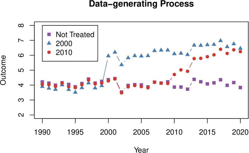
Figure 1: Example data with heterogeneous and dynamic treatment effects. Each line represents the average outcome in a given year for each group. In the absence of treatment, all three groups would exhibit parallel trends.

First, we will calculate a static difference-in-differences estimate using the did2s function.

static = did2s(    data = df_het,    yname = "dep_var",    treatment = "treat",    first_stage = ~ 0 | unit + year,    second_stage = ~ i(treat, ref = FALSE),    cluster_var = "unit",    verbose = FALSE)summary(static)

#> OLS estimation, Dep. Var.: dep_var#> Observations: 155,000#> Standard-errors: Custom#>             Estimate Std. Error t value  Pr(>|t|)#> treat::TRUE  2.25957   0.011705 193.037 < 2.2e-16 ***#> ---#> Signif. codes:  0 ’***’ 0.001 ’**’ 0.01 ’*’ 0.05 ’.’ 0.1 ’ ’ 1#> RMSE: 1.04088   Adj. R2: 0.513594

Since the returning object is a fixest object, all the accompanying output commands from fixest are available to use. For example, we can create regression tables:

fixest::etable(static, fitstat = c("n"), tex = TRUE,               title = "Estimate of Static TWFE Model",               notes = "Standard errors clustered at unit level.Estimated using Two-Stage Difference-in-Differences.proposed by Gardner (2021).")

Table 1: Estimate of Static TWFE Model

Dependent Variable:	dep_var
Model:	(1)
Variables
treat $=$ TRUE	2.260∗∗∗
	(0.0117)
Fit statistics
Observations	155,000
Custom standard-errors in parentheses
Signif. Codes: ***: 0.01, **: 0.05, *: 0.1

Standard errors clustered at unit level. Estimated using Two-Stage Difference-in-Differences. proposed by Gardner (2021).

However, since there are dynamic treatment effects in this example, it is much better to estimate the dynamic effects themselves using an event-study specification. We will then plot the results using fixest::iplot, which plots coefficients corresponding to an i() variable. Note that rel_year is coded as Inf for never-treated units, so this has to be noted in the reference part of the formula.

es = did2s(    data = df_het,    yname = "dep_var",    treatment = "treat",    first_stage = ~ 0 | unit + year,    second_stage = ~ i(rel_year, ref = c(-1, Inf)),    cluster_var = "unit",    verbose = FALSE)fixest::iplot(    es,    main = "Event study: Staggered treatment",    xlab = "Relative time to treatment",    col = "steelblue", ref.line = -0.5)# Add the (mean) true effectstrue_effects = tapply((df_het$te + df_het$te_dynamic), df_het$rel_year, mean)true_effects = head(true_effects, -1)points(-20:20, true_effects, pch = 20, col = "grey60")# Legendlegend(x=-20, y=3, col = c("steelblue", "grey60"),       pch = c(20, 20),       legend = c("Two-stage estimate", "True effect"))

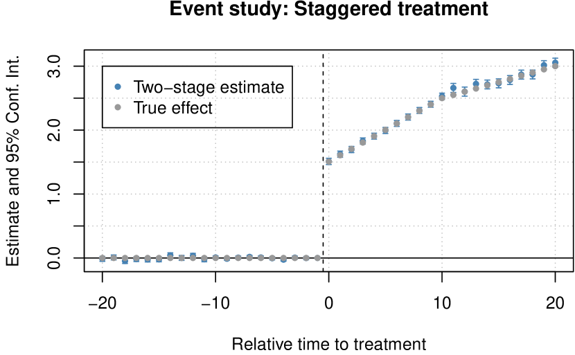
Figure 2: Event-study Estimate of TWFE Model. Standard Errors clustered at unit level. Estimated using the Two-Stage Difference-in-Differences proposed by Gardner (2021).

The event study estimates are found in Figure 2 and match closely to the true average treatment effects. For comparison to traditional OLS estimation of the event-study specification, Figure 3 plots point estimates from both methods. As pointed out by Sun and Abraham (2020), treatment effect heterogeneity between groups biases the estimated pre-trends. In the figure below, the OLS estimates appear to show violations of pre-trends even though the data was simulated under parallel pre-trends.

twfe = feols(dep_var ~ i(rel_year, ref=c(-1, Inf)) | unit + year, data = df_het)fixest::iplot(list(es, twfe), sep = 0.2, ref.line = -0.5,      col = c("steelblue", "#82b446"), pt.pch = c(20, 18),      xlab = "Relative time to treatment",      main = "Event study: Staggered treatment (comparison)")# True Effectspoints(-20:20, true_effects, pch = 20, col = "grey60")# Legendlegend(x=-20, y=3, col = c("steelblue", "#82b446", "grey60"), pch = c(20, 18, 20),       legend = c("Two-stage estimate", "TWFE", "True Effect"))

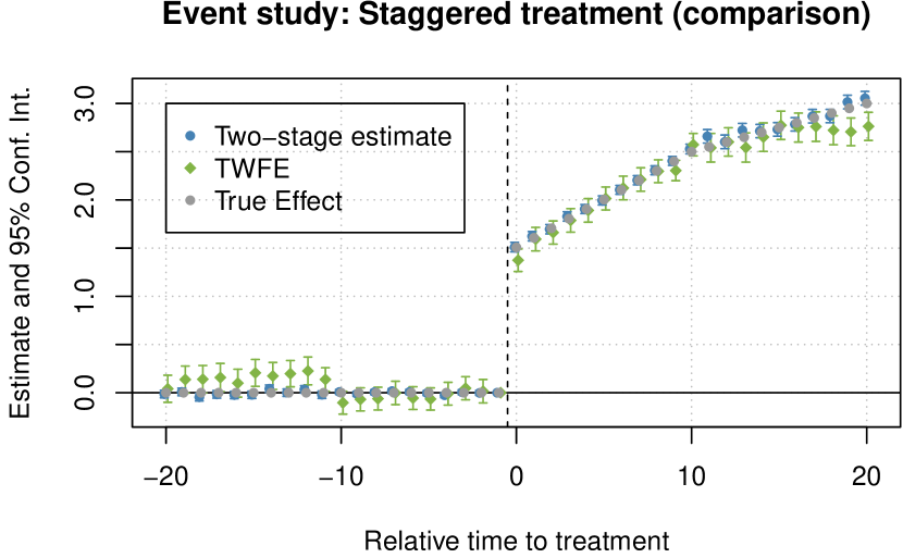
Figure 3: Event-study Estimate of TWFE Model. Standard Errors clustered at unit level. Estimated using the Two-Stage Difference-in-Differences proposed by Gardner (2021) and a Traditional TWFE model.

The event_study and plot_event_study command

The command event_study presents a common syntax that estimates the event-study TWFE model for treatment-effect heterogeneity robust estimators recommended by the literature and returns all the estimates in a data.frame for easy plotting by the command plot_event_study. The general syntax is

event_study(    data, yname, idname, tname, gname,    estimator,    xformla = NULL, horizon = NULL, weights = NULL)

The option data specifies the data set that contains the variables for the analysis. The four other required options are all names of variables: yname corresponds with the outcome variable of interest; idname is the variable corresponding to the (unique) unit identifier, $i$; tname is the variable corresponding to the time period, $t$; and gname is a variable indicating the period when treatment first starts (group status).

Table 2: Event Study Estimators

Estimator	R package /	Type	Comparison group	Main Assumptions	Uniform inference
	estimator argument
Gardner (2021)	did2s	Imputes $Y(0)$	Not-yet- and/or Never-treated	• Parallel Trends for all units • Limited anticipation∗ • Correct specification of $Y(0)$
Borusyak, Jaravel, and Spiess (2021)	didimputation	Imputes $Y(0)$	Not-yet- and/or Never-treated	• Parallel Trends for all units • Limited anticipation∗ • Correct specification of $Y(0)$
Callaway and Sant’Anna (2021)	did	2$\times$2 Aggregation	Either Not-yet- or Never-treated	• Parallel Trends for Not-yet-treated or Never-treated • Limited anticipation∗	Yes
Sun and Abraham (2020)	fixest/sunab	2$\times$2 Aggregation	Not-yet- and/or Never-treated	• Parallel Trends for all units • Limited anticipation∗
Roth and Sant’Anna (2021)	staggered	2$\times$2 Aggregation	Not-yet-treated	• Treatment timing is random • Limited anticipation∗

• This table summarizes the differences between various proposed event-study estimators in the econometric literature.

• Anticipation can be accounted for by adjusting ’initial treatment day’ back $x$ periods, where $x$ is the number of periods before treatment that anticipation can occur.

There are five main estimators available and the choice is specified for the estimator argument and are described in Table 2. The following paragraphs will aim to highlight the differences and commonalities between estimators. These estimators fall into two broad categories of estimators. First, did2s and didimputation (Butts, 2021) are imputation-based estimators as described above. Both rely on “residualizing” the outcome variable $\tilde{Y}=Y_{it}-\hat{\mu}_{g}-\hat{\eta}_{t}$ and then averaging those $\tilde{Y}$ to estimate the event-study average treatment effect $\tau^{k}$. These two estimators return identical point estimates, but differ in their asymptotic regime and hence their standard errors.

The second type of estimator, which we label 2x2 aggregation, takes a different approach for estimating event-study average treatment effects. The packages did (Callaway and Sant’Anna, 2021), fixest and staggered (Roth and Sant’Anna, 2021) first estimate $\tau_{gt}$ for all group-time pairs. To estimate a particular $\tau_{gt}$, they use a two-period (periods $t$ and $g-1$) and two-group (group $g$ and a “control group”) difference-in-differences estimator, known as a 2x2 difference-in-differences. The particular “control group” they use will differ based on estimator and is discussed in the next paragraph. Then, the estimator manually aggregate $\tau_{gt}$ across all groups that were treated for (at least) $k$ periods to estimate the event-study average treatment effect $\tau^{k}$.

These estimators do not all rely on the same underlying assumptions, so the rest of the table summarizes the primary differences between estimators. The comparison group column describes which units are utilized as comparison groups in the estimator and hence will determine which units need to satisfy a parallel trends assumption. For example, in some circumstances, treated units will look very different from never-treated units. In this case, parallel trends may only hold between ever-treated units and hence only these units should be used in estimation. In other cases, for example if treatment is assigned randomly, then it’s reasonable to assume that both not-yet- and never-treated units would all satisfy parallel trends.

For estimators labeled “Not-yet- and/or never-treated”, the default is to use both not-yet- and never-treated units in the estimator. However, if all never-treated units are dropped from the data set before using the estimator, then these estimators will use only not-yet-treated groups as the comparison group. did provides an option to use either the not-yet- treated or the never- treated group as a comparison group depending on which group a researcher thinks will make a better comparison group. staggered will automatically drop units that are never treated from the sample and hence only use not-yet-treated groups as a comparison group.

The next column, Main Assumptions, summarize concisely the main theoretical assumptions underlying each estimator. First, the assumptions about parallel trends match the previous discussion on the correct comparison group. The only estimator that doesn’t rely on a parallel trends assumption is staggered which relies on the assumption that when a unit receives treatment is random.

The next assumption, that is common across all estimators, is that there should be “limited anticipation” of treatment. In general, anticipatory effects are when units respond to treatment before it is actually implemented. For example, this can be common if the news of a policy triggers behavior responses before the treatment is put in place. “Limited anticipation” is when these anticipatory effects can only exist in a “few” pre-periods. In any of these cases, “treatment” should be manually moved back by the maximum number of periods where anticipation can occur. For example, if treatment starts in 2012 and anticipatory effects are reasonably only possible 2 years before, this units’ “group” should be labeled as 2010 in the data.

The imputation-based estimators require an additional assumption that the parametric model of $Y(0)=\mu_{i}+\eta_{t}+\varepsilon_{it}$ is correctly specified. This is because in the first stage, you have to accurately impute $Y(0)$ when residualizing $Y$ which relies on the correct specification of $Y(0)$. The 2x2 aggregation models do not estimate a parametric form of $Y(0)$ and hence only relies on a parallel trends assumption. The last column highlights that did allows for uniform inference of estimates. This addresses the problem that multiple hypotheses tests are being done by researchers (e.g. checking individually if all post periods are significant) by creating standard errors that adjust for multiple testing.

Example usage of event_study

The result of event_study is a tibble in a tidy format (Robinson et al., 2021) that contains point estimates and standard errors for each relative time indicator for each estimator. The results of event_study are stored as a dataframe with event-study term, the estimate, standard error, and a column containing which estimator is used for that estimate. This output dataframe will in turn be passed to plot_event_study for easy comparison. plot_event_study will return a ggplot object (Wickham, 2016). We return to the df_het dataset to see example usage of these functions.

data(df_het, package = "did2s")out = event_study(  data = df_het, yname = "dep_var", idname = "unit",  tname = "year", gname = "g", estimator = "all")

#> Estimating TWFE Model

#> Estimating using Gardner (2021)

#> Estimating using Callaway and Sant’Anna (2020)

#> Estimating using Sun and Abraham (2020)

#> Estimating using Borusyak, Jaravel, Spiess (2021)

#> Estimating using Roth and Sant’Anna (2021)

head(out)

#>    estimator  term   estimate  std.error#>       <char> <num>      <num>      <num>#> 1:      TWFE   -20 0.04097725 0.07167704#> 2:      TWFE   -19 0.13665695 0.07147683#> 3:      TWFE   -18 0.14015820 0.07245520#> 4:      TWFE   -17 0.15793252 0.07431871#> 5:      TWFE   -16 0.09910002 0.07379570#> 6:      TWFE   -15 0.20561127 0.07116478

plot_event_study(out, horizon = c(-5,10))

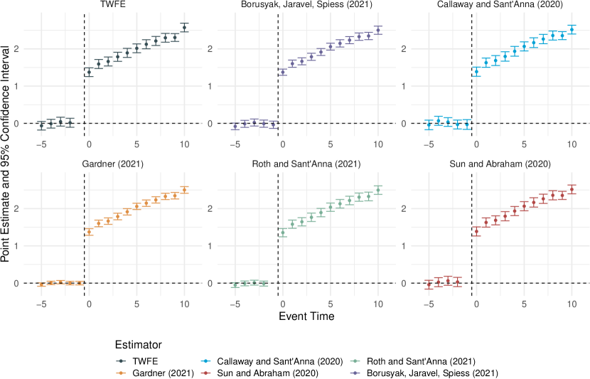
Figure 4: Event-study Estimators. This figure plots the results from the event_study command on example data.

Conclusion

This article introduced the package did2s which provides a fast, memory-efficient, and treatment-effect heterogeneity robust way to estimate two-way fixed-effect models. The package also includes the event_study and plot_event_study functions to allow for a single syntax for the various estimators introduced in the literature. A companion package in Stata is also available with similar syntax for the did2s function.

While this package includes an event_study function that aims to help individuals implement any of the proposed modern “solutions” to the difference-in-differences estimation, further research on this topic is needed to help practitioners be able to more precisely determine which estimators work best in their settings. Potentially, there could be data-driven methods to try to identify the plausibility of the different assumptions. Additionally, there is still more work to be done to formalize under what conditions covariates can flexibly be used in estimation. There is some initial work from Caetano et al. (2022), but there does not yet exist statistical software to perform their proposed estimator.

Kyle Butts
University of Colorado Boulder

https://www.kylebutts.com/
ORCiD: 0000-0002-9048-8059
buttskyle96@gmail.com

John Gardner
University of Mississippi

https://jrgcmu.github.io/
jrgardne@olemiss.edu

References

- Bergé (2018) L. Bergé. Efficient estimation of maximum likelihood models with multiple fixed-effects: the R package FENmlm. CREA Discussion Papers, (13), 2018.
- Borusyak et al. (2021) K. Borusyak, X. Jaravel, and J. Spiess. Revisiting event study designs: Robust and efficient estimation. Technical report, 2021.
- Butts (2021) K. Butts. didimputation: Difference-in-Differences estimator from Borusyak, Jaravel, and Spiess (2021), 2021. URL https://www.github.com/kylebutts/didimputation.
- Caetano et al. (2022) C. Caetano, B. Callaway, S. Payne, and H. S. Rodrigues. Difference in differences with time-varying covariates. Technical report, Feb 2022. URL http://arxiv.org/abs/2202.02903.