Holographic bottomonium formation in a cooling strong-interaction medium at finite baryon density

Abstract

The shrinking of the bottomonium spectral function towards narrow quasi-particle states in a cooling strong-interaction medium at finite baryon density is followed within a holographic bottom-up model. The 5-dimensional Einstein-dilaton-Maxwell background is adjusted to lattice-QCD results of sound velocity and susceptibilities. The zero-temperature bottomonium spectral function is adjusted to experimental $\Upsilon$ ground-state mass and first radial excitations. At baryo-chemical potential $\mu_{B}=0$, these two pillars let emerge the narrow quasi-particle state of the $\Upsilon$ ground state at a temperature of about 150 MeV. Excited states are consecutively formed at lower temperatures by about 10 (20) MeV for the $2S$ ($3S$) vector states. The baryon density, i.e. $\mu_{B}>0$, pulls that formation pattern to lower temperatures. At $\mu_{B}=200$ MeV, we find a shift by about 15 MeV.

I Introduction

The observation of sequential bottomonium suppression Chatrchyan:2012lxa ; Sirunyan:2017lzi ; Sirunyan:2018nsz ; Acharya:2018mni ; Acharya:2020kls in relativistic heavy-ion collisions at LHC has sparked a series of dedicated investigations, e.g. Aronson:2017ymv ; Du:2017qkv ; Hoelck:2016tqf ; Wolschin:2020kwt ; Yao:2018sgn ; Yao:2020xzw ; Yao:2020xwx ; Strickland:2019ukl ; Brambilla:2020qwo . Such heavy-quark flavor degrees of freedom receive currently some interest as valuable probes of hot and dense strong-interaction matter produced in heavy-ion collisions at LHC energies. The information encoded, e.g. in heavy quarkonia ($\bar{Q}Q=c\bar{c}$ or $b\bar{b}$) observables, supplements penetrating electromagnetic probes and hard (jet) probes and the rich flow observables, thus complementing each other in characterizing the dynamics of quarks and gluons up to the final hadronic states (cf. contributions in Proceedings:2019drx for the state of the art). Heavy quarks emerge essentially in early, hard processes, that is, they witness the course of a heavy-ion collision – either as individual entities or subjects of dissociating and regenerating bound states. Accordingly, the heavy-quark physics addresses such issues as charm ($c$, $\bar{c}$) and bottom ($b$, $\bar{b}$) dynamics related to transport coefficients Prino:2016cni ; Rapp:2018qla ; Xu:2018gux ; Cao:2018ews ; Brambilla:2019tpt ; Brambilla:2020qwo ; Song:2019cqz in the rapidly evolving and highly anisotropic ambient quark-gluon medium Chattopadhyay:2019jqj ; Bazow:2013ifa as well as $\bar{Q}Q$ states as open quantum systems Katz:2015qja ; Blaizot:2017ypk ; Blaizot:2018oev ; Brambilla:2017zei . The wealth of experimental data from LHC, and also from RHIC, enables a tremendous refinement of our understanding of heavy-quark dynamics. For a recent survey on the quarkonium physics we refer the interested reader to Rothkopf:2019ipj .

The yields of various hadron species, light nuclei and anti-nuclei emerging from heavy-ion collisions at LHC energies are well described by the thermo-statistical hadronization model Braun-Munzinger:2018hat ; Andronic:2017pug over an interval of nine orders of magnitude. The final hadrons and nuclear clusters are determined by two parameters: the freeze-out temperature $T_{fo}\approx 155$ MeV and a freeze-out volume depending on the system size or centrality of the collision. Due to the near-perfect matter-antimatter symmetry at top LHC energies the baryo-chemical potential $\mu_{B}$ is exceedingly small, $\mu_{B}/T_{fo}\ll 1$. While the authors of Reichert:2020yhx see a delicate interplay of elastic and inelastic hadron reactions as governing principle of the hadro-chemical freeze-out, it is argued in Andronic:2017pug that the freeze-out of color-neutral objects happens just in the demarcation region of hadron matter to quark-gluon plasma, i.e. confined vs. deconfined strong-interaction matter. In fact, lattice QCD results report a pseudo-critical temperature of $T_{pc}=(156\pm 1.5)$ MeV Bazavov:2018mes and $(158.0\pm 0.6)$ MeV Borsanyi:2020fev – values agreeing with the disappearance of the chiral condensates and the maximum of some susceptibilities. The key is the adjustment of physical quark masses and the use of 2+1 flavors Borsanyi:2013bia ; Bazavov:2014pvz , in short QCD₂₊₁(phys). Details of the coincidence of deconfinement and chiral symmetry restoration are matter of debate Suganuma:2017syi . Reference Bellwied:2018tkc advocates flavor-dependent freeze-out temperatures. Note that at $T_{pc}$ no phase transition happens, rather the thermodynamics is characterized by a cross-over accompanied by a pronounced nearby minimum of the sound velocity. This situation continues to non-zero baryon density as long as the baryo-chemical potential $\mu_{B}$ is small, $\mu_{B}/T_{pc}\ll 1$.

Among the tools for describing hadrons as composite strong-interaction systems is holography. Anchored in the famous AdS/CFT correspondence, holographic bottom-up approaches have facilitated a successful description of mass spectra, coupling strengths/decay constants etc. of various hadron species. While the direct link to QCD by a holographic QCD-dual or rigorous top-down formulations are still missing, one has to restrict the accessible observables to explore certain frameworks and scenarios. We consider here a framework which merges for the first time (i) QCD₂₊₁(phys) thermodynamics described by a dynamical holographic gravity-dilaton-Maxwell background and (ii) holographic probe quarkonia. We envisage a scenario which embodies QCD thermodynamics of QCD₂₊₁(phys) and the emergence of hadron states at $T_{c}$ at the same time. One motivation of our work is the exploration of a holographic model which is in agreement with the above hadron phenomenology in heavy-ion collisions at LHC energies. Early holographic studies Colangelo:2012jy ; Colangelo:2009ra ; Colangelo:2008us to hadrons at finite temperatures faced the problem of meson melting at temperatures significantly below the deconfinement temperature $T_{pc}$. Several proposals have been made Zollner:2016cgc ; Zollner:2017fkm ; Zollner:2017ggh to find rescue avenues which accommodate hadrons at and below $T_{pc}$. Otherwise, a series of holographic models of hadron melting without reference to realistic QCD thermodynamics, e.g. Braga:2015lck ; Braga:2016wkm ; Fujita:2009wc ; Fujita:2009ca ; Grigoryan:2010pj ; Braga:2017bml ; Braga:2019xwl ; Braga:2017oqw ; MartinContreras:2021bis – mostly with emphasis on quarkonium melting –, finds quarkonia states well above, at and below $T_{pc}$ in agreement with lattice QCD results Bazavov:2014cta ; Kim:2018yhk ; Ding:2019kva ; Larsen:2019zqv . It is therefore tempting to account for the proper QCD-related background.

In the temperature region $T={\cal O}(T_{pc})$, the impact of charm and bottom degrees of freedom on the quark-gluon–hadron thermodynamics is minor Borsanyi:2016ksw . Thus, we consider quarkonia, in particular bottomonium, as test particles. We follow Gubser:2008ny ; Finazzo:2014cna ; Finazzo:2013efa ; Zollner:2018uep and model the holographic background by a gravity-dilaton set-up supplemented by a Maxwell field DeWolfe:2010he ; DeWolfe:2011ts , i.e. without adding further fundamental degrees of freedom to the dilaton. That is, the dilaton potential and its coupling to the Maxwell field are adjusted to QCD₂₊₁(phys) lattice data. Our emphasis is here on the formation of bottomonium in a cooling strong-interaction environment. Thereby, the bottomonium properties are described by a spectral function. The primary aim of the present paper is to study the impact of a finite baryon density of the strong-interaction medium, thus complementing Zollner:2020cxb ; Zollner:2020nnt . Finite baryon effects become relevant at smaller beam energies, e.g. at RHIC, and are systematically accessible in the beam energy scans Odyniec:2019kfh ; Abdallah:2021fzj ; Bzdak:2019pkr . We restrict ourselves to equilibrium and leave non-equilibrium effects, e.g. Bellantuono:2017msk ; Yao:2017fuc , for future work.

Such $\mu_{B}>0$ effects on holographic bottomonium spectroscopy have been considered, e.g. in Braga:2017oqw ; Braga:2019xwl ; Braga:2020myi . Our present investigation is distinguished by choosing a holographic bottom-up background which is adjusted to QCD-lattice data of sound velocity and susceptibilities in the temperature range 100 MeV $<T<$ 600 MeV. That is, the gravity-dilaton-Maxwell fields are dynamically determined by solutions of the Einstein equations consistent with the equations of motion of dilaton and Maxwell fields. We do not touch the large-$\mu_{B}$ region or a conjectured critical point DeWolfe:2010he ; DeWolfe:2011ts ; Rougemont:2015wca ; Critelli:2017oub ; Knaute:2017opk ; Knaute:2017lll ; Grefa:2021qvt since the experimental access to bottomonium physics is expected to be feasible at not too small beam energies, i.e. at low-values of $\mu_{B}$ in the central rapidity region.

Our paper is organized as follows. In Section II, the dynamics of the probe quarkonia is formulated, and the coupling to the thermodynamics-related background is explained in Section III. Both ingredients are joint in Section IV for the calculation of the spectral functions. The numerical results for the bottomonium states $\Upsilon(1S,2S,3S)$ are presented in Section V. We summarize in Section VI. Appendix A details the field equations for the Einstein-dilaton-Maxwell model with radial bulk coordinate $z$. Appendix B considers some options for UV-IR matching to generate within holography the $\Upsilon(nS)$ $I^{G}(J^{PC})=0^{-}(1^{--})$ spectrum.

II Bottom-up model for quarkonia

In thermal equilibrium, the admixture of equilibrated heavy quarks in strong-interaction matter at $T<250$ MeV is small Borsanyi:2016ksw ; Bellwied:2015lba . Rather, initial hard parton interactions (essentially gluon fusion) create heavy quarks in heavy-ion collisions. Thus, heavy quark pairs serve as test particles and need not to be back-reacted. In particular, quarkonia constituents are decoupled from the ambient quark content, with the exception of the gluon component. In a model with minimalistic field content one would prefer to keep the effective gravity-dilaton background (extended by the Maxwell field ${\cal B}$ for mimicking $\mu_{B}>0$) to catch QCD thermodynamics and attribute to the test particles solely one vector field ${\cal A}$. A $U(1)$ gauge field ${\cal A}(z)$ in the bulk is supposed to be the dual of the vector meson current operator $\bar{Q}\gamma^{\mu}Q$ at the boundary. The string-frame action is accordingly

$$S_{m}^{V}=\frac{1}{k_{V}}\int\mathrm{d}^{4}x\,\mathrm{d}z\sqrt{g_{5}}\,\frac{1}{4}e^{-\phi_{m}}\,F_{\cal A}^{2},\quad\phi_{m}:=\phi-\log G_{m}(\phi),$$ (1)

where $F_{\cal A}$ stands for the Abelian field-strength tensor of ${\cal A}$ and $k_{V}=\frac{N_{c}}{24\pi^{2}}$ with number $N_{c}=3$ of colors.

In contrast to common previous practice, the background quantities $g_{5}$ (metric determinant) as well as $\phi$ (dilaton field) and ${\cal B}$ (Maxwell field) are universal for any test particle, therefore, $G_{m}$ encodes solely the essential properties of the respective test particle. We attribute the quarkonia masses to the considered test particle. Rather than including the heavy-quark masses explicitly, we encode them in the following manner in $G_{m}$. From the the ansatz ${\cal A}_{\mu}=\epsilon_{\mu}\,\varphi(z)\,\exp\{ip_{\nu}x^{\nu}\}$ with $\mu,\nu=0,\cdots,3$, which uniformly separates the $z$ dependence of the gauge field by the bulk-to-boundary propagator $\varphi$ for all components of ${\cal A}$, and the constant polarization vector $\epsilon_{\mu}$ and gauges ${\cal A}_{z}=0$ and $\partial^{\mu}{\cal A}_{\mu}=0$, the equation of motion follows from the action (1) as

$$\varphi^{\prime\prime}+\left[\frac{1}{2}A^{\prime}+(\partial_{\phi}\log G_{m}-1)\phi^{\prime}+(\log f)^{\prime}\right]\varphi^{\prime}+\frac{p^{\mu}p_{\mu}}{f^{2}}\varphi=0,$$ (2)

which is cast in the form of a one-dimensional Schrödinger equation with the tortoise coordinate $\xi$

$$\left[\partial_{\xi}^{2}-(U(z(\xi))-m_{n}^{2})\right]\psi_{n}(\xi)=0,\quad n=0,1,2,\cdots,$$ (3)

by the transformation $\psi(\xi)=\varphi(z(\xi))\,\exp\{\frac{1}{2}\int_{0}^{\xi}\mathrm{d}z\,{\cal S}(\xi)\}$ and $p^{\mu}p_{\mu}\to m_{n}^{2}$. One has to employ $z(\xi)$ from solving $\partial_{\xi}=(1/f)\partial_{z}$. The Schrödinger-equivalent potential in (3) is

$$U:=\left(\frac{1}{2}{\cal S}^{\prime}+\frac{1}{4}{\cal S}^{2}\right)f^{2}+\frac{1}{2}{\cal S}ff^{\prime}$$ (4)

as a function of $\xi(z)$ with

$${\cal S}:=\frac{1}{2}A^{\prime}-\phi^{\prime}+\partial_{z}\log G_{m}(\phi(z)).$$ (5)

A prime means the derivative w.r.t. the bulk coordinate $z$.

At $T=0$, we have $f=1$ and $\xi=z$, and $m_{n}$ in Eq. (3) is the quarkonium mass spectrum to be used as input. Therefore, the Schrödinger-equivalent potential $U(z)$ must be chosen in such a manner to deliver the wanted values of $m_{n}$. With given $U(z)$, the Ricatti equation (4) must be solved for ${\cal S}$, which in turn determines the heavy-quark mass-specific function $G_{m}(\phi)$ via Eq. (5). This $G_{m}(\phi)$ is assumed as independent of temperature and baryo-chemical potential, i.e. is ready for direct use at $T>0$ and $\mu_{B}>0$ as well.

In the described chain of operations for getting $G_{m}$, the zero-temperature background quantities $A(z)$ and $\phi(z)$ are needed. They are determined by the temperature independent dilation potential $V(\phi)$, which is adjusted to lattice-QCD thermodynamics data, briefly recalled in the next section.

III Background generated by the Einstein-dilaton-Maxwell bottom-up model

We follow here closely the Einstein-dilaton-Maxwell (EdM) model of Knaute:2017opk , see also Knaute:2017lll ; Critelli:2017oub ; Grefa:2021qvt . The EdM action reads

$$S_{EdM}=\frac{1}{2\kappa_{5}^{2}}\int\mathrm{d}^{4}x\,\mathrm{d}z\,\sqrt{-g_{5}}\left(R-\frac{1}{2}\partial^{M}\phi\,\partial_{M}\phi-V(\phi)-\frac{1}{4}{\cal F}(\phi)F_{{\cal B}}^{2}\right)+S_{GH},$$ (6)

where $R$ is the Einstein-Hilbert part, $F_{\cal B}^{MN}=\partial^{M}{\cal B}^{N}-\partial^{N}{\cal B}^{M}$ stands for the field strength tensor of Abelian gauge field ${\cal B}$ à la Maxwell with ${\cal B}_{M}\mathrm{d}x^{M}=\Phi(z)\,dt$ defining the electro-static potential, and $\phi$ is a real scalar (dilatonic) field with self-interaction described by the potential $V(\phi)$. The bulk Maxwell field is sourced by the conserved light-quark baryon-current $\bar{q}\gamma^{\mu}q$ at the boundary. In such manner, this field is related to baryon density effects, parameterized by $\mu_{B}$. The Maxwell field and dilaton are coupled by the dynamical strength function ${\cal F}(\phi)$ DeWolfe:2010he ; DeWolfe:2011ts . (Note the analogy of ${\cal F}(\phi)$ in (6) and $e^{-\phi_{m}}$ in (1).) The Gibbons-Hawking term $S_{GH}$ for a consistent formulation of the variational problem is not needed explicitly in our context. The numerical value of the “Einstein constant” $\kappa_{5}^{2}=8\pi G_{N}$ is irrelevant in our context. The metric determinant $g_{5}$ is related to the ansatz of the infinitesimal line element

$$\mathrm{d}s^{2}=g_{MN}\mathrm{d}x^{M}\mathrm{d}x^{N}:=\exp\{A(z,z_{H})\}\left[f(z,z_{H})\,\mathrm{d}t^{2}-\mathrm{d}\vec{x}^{2}-\frac{\mathrm{d}z^{2}}{f(z,z_{H})}\right],$$ (7)

with warp function $A$ and blackening function $f$, already used in Section II.

We relegate the field equations following from the action (6) in the coordinates (7) to Appendix A, but mention here the employed parameterizations

$$L^{2}V(\phi) = \left\{\begin{array}[]{l}-12\exp\{\frac{1}{2}a_{1}\phi^{2}+\frac{1}{4}a_{2}\phi^{4}\}\mbox{ for }\phi<\phi_{x},\\ a_{10}\cosh[a_{4}(\phi-a_{5})]^{a_{3}/a_{4}}\exp\{a_{6}\phi+\frac{a_{7}}{a_{8}}\tanh[a_{8}(\phi-a_{9})]\}\mbox{ for }\phi>\phi_{x},\end{array}\right.$$ (10)

$${\cal F}(\phi) = c_{0}+c_{1}\tanh[c_{2}(\phi-c_{3})]+c_{4}\exp\{-c_{5}\phi\}$$ (11)

and refer the interested reader to Knaute:2017opk for listings of the parameters $a_{1,\cdots,10}$, $\phi_{x}$, $c_{0,\cdots,5}$ etc. Figures 1 and 2 in Knaute:2017opk exhibit the excellent agreement with lattice-QCD data in the interval $T\in[100,500]$ MeV and remaining uncertainties due to limited precision, in particular of the sound velocity in the interval $T\in[100,160]$ MeV and the susceptibility $\chi_{4}$. The scale setting is accomplished by $L^{-1}=5.148$ GeV. The locus of the minimum sound velocity squared is described in leading order by $T_{min\{v_{s}^{2}\}}(\mu_{B})=T_{v_{s}^{2}}(\mu_{B}=0)\left[1-\kappa\left(\displaystyle\frac{\mu_{B}}{T_{v_{s}^{2}}(\mu_{B}=0)}\right)^{2}\right]$ with $T_{v_{s}^{2}}(\mu_{B}=0)=145$ MeV and $\kappa=0.0178$ MeV. Note that $T_{v_{s}^{2}}(\mu_{B}=0)<T_{pc}$. Despite the direct relation to an observabe, the location of $min\{v_{s}^{2}\}$ is not so precisely constrained by lattice-QCD data as that of the maximum of chiral susceptibility which determines quite accurately $T_{pc}$ Bazavov:2018mes ; Borsanyi:2020fev . In so far, the curves $T_{min\{v_{s}^{2}\}}(\mu_{B})$ and $T_{pc}(\mu_{B})$ need not to coincide.

The EdM model with these input data is then ready to transport the thermodynamic information from $\mu_{B}=0$ to $\mu_{B}>0$, thus uncovering the $T$-$\mu_{B}$ plane. This is very much the spirit of the quasi-particle model Peshier:1999ww ; Peshier:2002ww , where a flow equation facilitates such a transport.

IV Spectral functions

The equation of motion (2) of $\varphi$ can also be employed to compute quarkonia spectral functions, cf. Colangelo:2012jy ; Fujita:2009wc ; Fujita:2009ca ; Grigoryan:2010pj ; Hohler:2013vca ; Teaney:2006nc . For $\omega^{2}=p^{\mu}p_{\mu}>0$ fixed, the asymptotic boundary behavior facilitates two linearly independent solutions by considering the leading-order terms on both sides of the interval $[0,z_{H}]$. (i) For $z\to 0^{+}$, one has the general solution $\varphi(z\to 0)\to A(\omega)\varphi_{1}+B(\omega)\varphi_{2}$, due to the AdS asymptotic at the boundary, with two $\omega$-dependent complex constants $A$ and $B$, and $\varphi_{1}(z\to 0)\to 1$ and $\varphi_{2}(z\to 0)\to(z/z_{H})^{2}$. (ii) Near the horizon, $z\to z_{H}^{-}$, the asymptotic behavior of solutions of (2) is steered by the poles of $1/f$ and $1/f^{2}$. The two linearly independent solutions are $\varphi_{\pm}(z\to z_{H})\to(1-\frac{z}{z_{H}})^{\pm i\omega/|f^{\prime}(z_{H})|}$, where $\varphi_{\pm}$ represent out-going and in-falling solutions, respectively. The general near-horizon solution is given by $\varphi(z\to z_{H})\to C(\omega)\varphi_{(}z)++D(\omega)\varphi_{-}(z)$, again with complex constants $C$ and $D$ which depend on $\omega$. The side conditions for the bulk-to-boundary propagator are $\varphi(0)=1$, which means $A(\omega)=1$, and $\varphi(z\to z_{H})=\varphi_{-}(z\to z_{H})$ (purely in-falling solution at the black hole horizon), yielding $C(\omega)=0$. Due to the bilinear mapping $(A,B)\mapsto(C,D)$, the value of $B$ for getting the desired in-falling solution can be determined by solving the above equations twice, once with $A=1$, $B=0$ and once with $A=0$, $B=1$ and comparing the result with $\varphi_{-}$ to dig out the proper coefficients.

The corresponding retarded Green function $\mathcal{G}^{\rm R}$ of the dual current operator $\bar{Q}\gamma_{\mu}Q$, defined within the framework of the holographic dictionary via a generating functional by $\mathcal{G}^{\rm R}=\frac{\delta^{2}}{\delta{\cal A}^{0\,\mu}(-\omega)\delta{\cal A}^{0}_{\mu}(\omega)}\langle\exp\{i\int\mathrm{d}^{4}x\,{\cal A}^{0}_{\nu}\bar{Q}\gamma^{\nu}Q\}\rangle$, is given by

$$\mathcal{G}^{\rm R}(\omega)=\frac{\delta^{2}S_{m}^{V,\,\mbox{on-shell}}}{\delta\mathcal{A}^{0\,\mu}(-\omega)\,\delta\mathcal{A}^{0}_{\mu}(\omega)}=\frac{1}{k_{V}}\lim\limits_{z\to 0}\frac{1}{z}\varphi^{*}(z)\varphi^{\prime}(z)=\frac{2}{k_{V}z_{H}^{2}}B(\omega)$$ (12)

with $\mathcal{A}^{0}_{\mu}\equiv\epsilon_{\mu}\exp\{ip_{\nu}x^{\nu}\}$ for $\mu\in\{1,2,3\}$ Teaney:2006nc . The quantity $S_{m}^{V,\,\mbox{on-shell}}$ denotes here the action (1) with the solution $\varphi$ from (2). Finally, the spectral function $\rho$ follows from $\rho(\omega)=\mbox{Im}\,\mathcal{G}^{\rm R}(\omega)=\frac{2}{k_{V}z_{H}^{2}}\mbox{Im}\,B(\omega)$. It has the dimension of energy squared, suggesting to use $L^{2}\rho$ or $\rho/\omega^{2}$ as convenient representations.

V Numerical results

The spectral function $\rho(\omega,T,\mu_{B})$ is accessible by numerical means by the following chain of operations: (i) solving the equations of motion (13 - 16) following from the action (6) with boundary conditions (17 - 22) for the background encoded in $A_{0}(z)$, $f_{0}(z)=1$, $\phi_{0}(z)$ with the prescribed $V(\phi_{0})$ from Eq. (10) yields the input for Eqs. (4, 5) for the determination of $G_{m}(\phi)$ at $T=0$ (highlighted by the subscript “0”, using $U_{0}$ from Appendix B; for parameter values, see Appendix B.2), (ii) using afterwards that $G_{m}(\phi)$ in Eqs. (2, 12) but with $A(z;z_{H})$, $f(z;z_{H})$, $\phi(z,z_{H})$ determined again by $V(\phi)$ via the equations of motion(13 - 16) following from the action (6) with boundary conditions (17 - 22) and ${\cal F}(\phi)$ from Eq. (11), see Appendix A. Some care is needed in that numerical treatment.

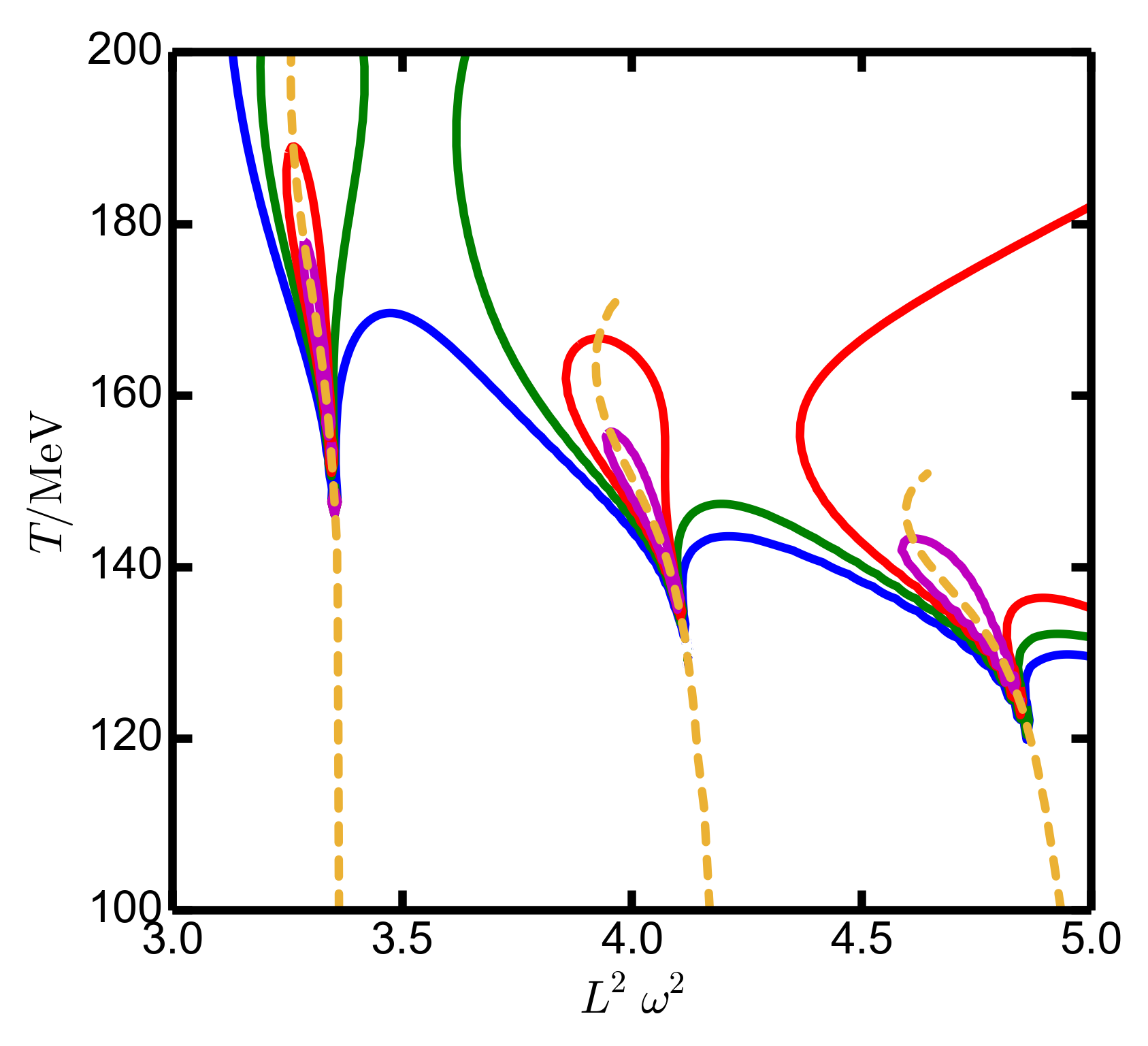
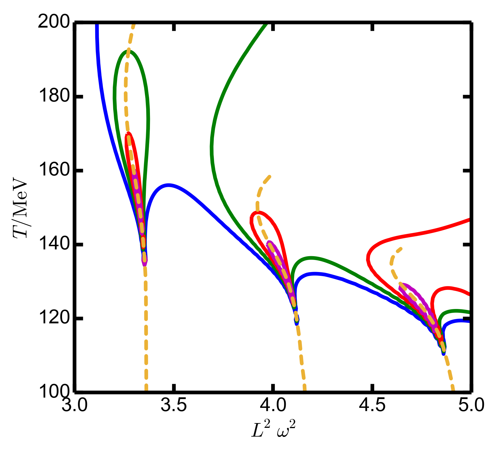
Figure 1: Contour plots of the $\Upsilon$ spectral function $L^{2}\rho(\omega,T,\mu_{B})$ over the temperature vs. scaled frequency $L^{2}\omega^{2}$ plane for $\mu_{B}=0$ (left), 100 MeV (middle) and 200 MeV (right); blue, green, red and magenta contour curves correspond to $L^{2}\rho=1$, 3, 10 and 30. The dashed orange curves mark the maximum positions of $L^{2}\rho(\omega,T,\mu_{B})$ w.r.t. $\omega$. At large temperatures, such local maxima disappear and the respective state can be considered as completely molten. At lower temperatures, sharp quasi-particles have been formed, i.e. the contours are squeezed and are hidden behind the dashed orange curves.

Figure 2: $\Upsilon$ spectral function $L^{2}\rho(\omega,T,\mu_{B})$ as a function of scaled frequency $L^{2}\omega^{2}$ for $\mu_{B}=0$ (left), 100 MeV (middle) and 200 MeV (right) at 155 MeV (red), 150 MeV (green) and 145 MeV (blue). These plots arise from Fig. 1 as cross sections at constant temperature.

Figure 3: Scaled $\Upsilon$ spectral function $\rho(\omega,T,\mu_{B})/\omega^{2}$ as a function of energy $\omega$ for $T=145$ MeV (left, i.e. at $T/T_{v_{s}^{2}}=1$), 150 MeV (middle) and 155 MeV (right, i.e. at $T\approx T_{pc}$) at $\mu_{B}=0$ (blue), 100 MeV (green) and 200 MeV (red). The data of Fig. 2 is rearranged to highlight the $\mu_{B}$ dependence and to furnish a comparison with experimental results which use $M_{\mu^{+}\mu^{-}}$ as abscissa.

Our results are exhibited in Fig. 1 for the $\Upsilon$ meson. We emphasize that neither an explicit quark-mass dependence enters our approach (instead, quark masses are implicitly accounted via $U_{0}(z)$ for entering $G_{m}$) nor a confinement criterion (instead, narrow spectral functions as quasi-particle states are considered as confined $J^{PC}=1^{--}$ $\bar{b}b$ states). In so far, the emergence of such narrow quasi-particle ground states at $T={\cal O}(T_{pc})$ is astonishing. The higher the excitation, the later the excited-state formation happens when considering the cooling due to expansion. The net effect of the finite baryon-chemical potential $\mu_{B}$ is a lowering of the formation temperature.

The density of low-mass color carriers is $\propto T^{3}+[\cdot]T^{2}\mu_{B}$ in leading order of small $\mu_{B}$ and species-dependent positive constant $[\cdot]$, i.e. increases with increasing $\mu_{B}$. In the spirit of the Matsui-Satz conjecture Matsui:1986dk , the color charge screening becomes stronger due to $\mu_{B}>0$, and the formation of bound states is delayed (suppressed) therefore in a cooling medium. A closer look on the contour curves at $T=140\cdots 160$ MeV suggests $\rho(\omega,T-15\leavevmode\nobreak\ \mbox{MeV},\mu_{B}=0)\approx\rho(\omega,T,\mu_{B}=200\leavevmode\nobreak\ \mbox{MeV})$, meaning that the $\Upsilon$ formation pattern is shifted down by a temperature of about 15 MeV by the impact of the baryo-chemical potential $\mu_{B}=200$ MeV. Otherwise, the minimum sound velocity, $T_{min\{v_{s}^{2}\}}(\mu_{B})$ drops only by about 5 MeV when going from $\mu_{B}=0$ to $\mu_{B}=200$ MeV. While being rather semi-quantitative and restricted to $\Upsilon$, this finding may be interpreted as a hint to $T_{fo}(\mu_{b})\neq T_{pc}(\mu_{b})$ at $\mu_{B}>0$.

Focusing on the crucial temperature region near $T_{pc}$ or $T_{v_{s}^{2}}$, one observes how rapidly the ground state evolves towards a sharp quasi-particle within this narrow interval of $T$ at $\mu_{B}=0$, see left sharp peak in left panel in Fig. 2. The first excitation (the middle peak) becomes clearly visible, with peak position noticeably shifting up upon dropping temperature. In contrast, the second excitation is identifiable at $T=145$ MeV but not so clearly at higher temperatures. These trends continue at $\mu_{B}>0$, see middle and right panels in Fig. 2. At $\mu_{B}=200$ MeV, the second excitation is not identifiable as clear peak down to $T=145$ MeV, while the first excitation sticks out only at $T\leq 150$ MeV. Let us emphasize that, at $\mu_{B}=0$, the first and (weakly) the second excitations are identifiable as peak structures, in contrast to MartinContreras:2021bis , where these excitations appear as molten, while the ground state persists up to high temperatures since it is kept by a narrow deep well potential.

To highlight the $\mu_{B}$ dependence, we exhibit in Fig. 3 the same spectral functions arranged in reversed order, i.e. various values of $\mu_{B}$ at a given temperature. Such a representation evidences the impact of the baryo-chemical potential in a clear manner. Note that in an adiabatically cooling strong-interaction system one should employ the isentropic curves $T(\mu_{B})$ to follow the evolution of the spectral function. Figure 3 provides some guidance for that.

Figure 4: The same data as in Fig. 2 is used but convoluted with a resolution function with width of 100 MeV (see the text) to enable a comparison with experimental results which use linear scales. An adaptive $\bar{\omega}$ grid with minimum spacing of $10^{-8}L$ is employed. Note that feeding is not included.

The relation of the spectral function to the resulting $\mu^{+}\mu^{-}$ spectrum from $\Upsilon\to\mu^{+}\mu^{-}$ may be elaborated as in previous studies, e.g. by superimposing the thermal yield (which needs a model of the space-time evolution of the fireball) and the post-freeze-out contribution (which is directly related to the $\Upsilon(nS)$ yields and feedings) and the various background sources. This is beyond the scope of our paper. Nevertheless, the emerging picture of our model (see $\mu_{B}=0$ curves in Fig. 3) appears at the fist glance qualitatively consistent with experimental observations Chatrchyan:2012lxa ; Sirunyan:2017lzi ; Sirunyan:2018nsz ; Acharya:2018mni . The strengths of excited states, $\Upsilon(2S,3S)$, are gradually suppressed w.r.t. to the ground state $\Upsilon(1S)$ in heavy-ion collisions with participant numbers $N_{part}>100$, most notably the $3S$ state, while in $pp$ collisions one clearly identifies $\Upsilon(2S,3S)$ as prominent peaks, albeit with decreasing strengths. One could imagine that convoluting our spectral functions with a finite (fiducial) resolution leads to a picture resembling better the observations, e.g. figure 1 in Chatrchyan:2012lxa . In fact, applying a Gaussian resolution function according to the scheme $\bar{\rho}_{\sigma}(\omega)=\int_{0}^{\infty}\mathrm{d}\bar{\omega}\,\bar{\rho}(\bar{\omega})\frac{1}{\sqrt{2\pi\sigma^{2}}}\exp\{-\frac{(\bar{\omega}-\omega)^{2}}{2\sigma^{2}}\}$ with $\bar{\rho}(\omega):=\rho(\omega)/\omega^{2}$ and selecting the ad hoc value $\sigma=0.1$ GeV generates a pattern closer to the observation, see Fig. 4. While the underlying soft-wall holographic potential captures approximately the mass spectrum of radial excitations at $T=0$, it facilitates, also in the present background, decay constants increasing with (or independent of) radial quantum number $n$, in contrast to experimental data. This imperfection seems to continue to $T>0$: the strengths of (i.e. yields from) excitations become too large. Therefore, we do not introduce a continuum or background subtraction, as discussed in MartinContreras:2021bis , and leave further refinements (e.g. the options offered in Appendix B.3 w.r.t. decay constants) and feeding corrections to follow-up work.

VI Conclusion and Summary

Using a bottom-up holographic model with minimalistic field content, we investigate the impact of the finite baryo-chemical potential $\mu_{B}$ on bottomonium formation at temperatures in the order of the hadron-chemical freeze-out in relativistic heavy-ion collisions. The model has two pillars: (i) the vector meson part which employs the bottomonium masses of ground state and radial excitations as input to adjust a suitable Schrödinger-equivalent potential, and (ii) the Einstein-dilaton-Maxwell background which is adjusted independently to lattice-QCD thermodynamics (sound velocity and light-quark susceptibilities). The field content is as follows: (i) a bottomonium-specific function $G_{m}(\phi)$, which encodes implicitly the $b$ quark masses via the Schrödinger-equivalent potential $U_{0}(z)$ and is essential for the bulk-to-boundary propagator $\varphi(z)$, and (ii) the gravity-dilaton-Maxwell part, determined dynamically by the dilaton potential $V(\phi)$ and the dilaton-Maxwell coupling ${\cal F}(\phi)$. Since there is neither a confinement criterion nor a chiral condensate as order parameter in such an approach, we consider the shrinking of the spectral function $\rho$ (determined by $\varphi$) to a narrow quasi-particle state as bottomonium formation in a cooling strong-interaction medium. Despite a simple two-parameter Schrödinger-equivalent potential $U_{0}$, we find the bottomonium ground-state formation at about a temperature of 150 MeV at $\mu_{B}=0$. Increasing $\mu_{B}$ drops the formation temperature. Excited states are consecutively formed at lower temperatures, or the spectral strengths are not yet concentrated completely at the $T=0$ quasi-particle energy at a given temperature. This fits well in the experimental observation that the $\Upsilon(2S)$ and $\Upsilon(3S)$ states are hardly identifiable in the di-lepton spectra in heavy-ion collisions ate LHC, while the ground state is clearly visible Chatrchyan:2012lxa . In contrast, $\Upsilon(1S,2S,3S)$ are clearly seen in proton-proton collisions at the same beam beam energies per nucleon.

Our approach assumes rapid thermalization and equilibration, since the cooling of the medium is handled as sequence of equilibrium states. Off-equilibrium phenomena up to dynamical freeze-out need to be considered in refined investigations. Highly desirable would be a closer contact to string theory to overcome the deployed phenomenological parameterizations steering our two pillars, background thermodynamics and vacuum mass spectrum.

Appendix A Using the bulk coordinate $\mathbf{z}$ in the EdM model

The equations of motion for the dilaton $\phi(z)$, the Maxwell field $\Phi(z)$ with the coupling function ${\cal F}(\phi)$, following from the action (6), read in the coordinates (7) with warp factor $\exp\{A(z)\}$ and blackening function $f(z)$

$$\phi^{\prime\prime} = -[\frac{3}{2}A^{\prime}+(\log f)^{\prime}]\phi^{\prime}-\frac{1}{f}[e^{A}\frac{\partial V(\phi)}{\partial\phi}+\frac{1}{8}\frac{\partial{\cal F}(\phi)}{\partial\phi}\Phi^{\prime 2}],$$ (13)

$$\Phi^{\prime\prime} = -[\frac{1}{2}A^{\prime}+\frac{1}{4}\frac{\log{\cal F}(\phi)}{\partial\phi}\phi^{\prime}]\Phi^{\prime},$$ (14)

$$A^{\prime\prime} = \frac{1}{2}A^{\prime 2}-\frac{1}{3}\phi^{\prime 2},$$ (15)

$$f^{\prime\prime} = -\frac{3}{2}A^{\prime}f^{\prime}-\frac{1}{4}{\cal F}(\phi)e^{-A}\Phi^{\prime 2}.$$ (16)

The leading-order initial conditions are (i) near boundary, i.e. $z\to 0^{+}$,

$$\lim_{z\to 0}\phi = 0,\hskip 82.51299pt\lim_{z\to 0}\phi^{\prime}=0,$$ (17)

$$\lim_{z\to 0}\Phi = \mu_{B}L,$$ (18)

$$\lim_{z\to 0}A = -2\log\frac{z}{L}+\cdots,\quad\lim_{z\to 0}A^{\prime}=-\frac{2}{z}+\cdots,$$ (19)

$$\lim_{z\to 0}f = 1,$$ (20)

and (ii) near horizon, i.e. $z\to z_{H}^{-}$,

$$\lim_{z\to z_{H}}\Phi =0,$$ (21)

$$\lim_{z\to z_{H}}f =0.$$ (22)

The Eqs. (21) and (22) make these equations a mixed boundary problem. The Hawking temperature is determined by $T(z_{H})=-\frac{1}{4\pi}f(z,z_{H})^{\prime}|_{z=z_{H}}$ with a freely chosen value of the horizon position $z_{H}$ and free choice of $\mu_{B}$. For completeness, we note also entropy density $s(T,\mu_{B})=\frac{2\pi}{\kappa_{5}^{2}}\exp\{\frac{3}{2}A(z_{H})\}$ and baryon density $n_{B}(T,\mu_{B})=-\frac{1}{\kappa_{5}^{2}}\Phi_{2}$ with $\Phi_{2}$ from the small-$z$ expansion $\Phi=\mu_{B}L+\Phi_{2}(z/L)^{2}+\cdots$.

References Knaute:2017opk ; Knaute:2017lll ; Critelli:2017oub ; Grefa:2021qvt use essentially the coordinates originally employed in DeWolfe:2010he ; DeWolfe:2011ts with special gauging of the radial coordinate. These solutions can be parameterized by the double $(\phi(z_{H}),\Phi(z_{H}))$ and need a posteriori the determination of the (screwed) $T$-$\mu_{B}$ mesh. The advantage of Eqs. (13 - 22) is in the boundary conditions (20) and (21), which make easier the scan of the $T$-$\mu_{B}$ plane.

Appendix B UV-IR matching

B.1 Generalities

In the zero-temperature limit, $T\to 0$ at $\mu_{B}=0$, one has $f\to 1$, $\xi\to z$ and $U\to U_{0}$ in Eq. (3). The primary request to any useful Schrödinger-equivalent potential $U_{0}(z)$ is to get the proper level spacing via

$$y^{\prime\prime}-(U_{0}-\hat{E}L^{-2})y=0.$$ (23)

A constant common shift of $U_{0}\to U_{0}^{b}=U_{0}+4b/L^{2}$ can be absorbed in $\hat{E}\to\hat{E}^{b}=\hat{E}+4b$ to accomplish the wanted meson ground-state mass squared, $L^{2}m_{0}^{(b)\,2}=\hat{E}_{0}+4b$, independent of $U_{0}(z)$. Here, we suppose that Eq. (23) delivers a set of discrete eigenvalues $\hat{E}_{n}\equiv L^{2}m_{n}^{2}$, $n=0,1,2,\cdots$ by the requirement of square-integrable solutions $y_{n}$.

We emphasize again hat $U_{0}(z)$ is an independent input in our approach which determines ${\cal S}_{0}$, via ${\cal S}_{0}^{\prime}{}^{2}+\frac{1}{2}{\cal S}_{0}^{2}-2U_{0}=0$ from Eq. (4), and $G_{m}(\phi_{0})$, via $(\log G_{m})^{\prime}-{\cal S}_{0}+\frac{1}{2}A_{0}^{\prime}-\phi_{0}^{\prime}=0$ from Eq. (5). (The needed holographic background quantities $A_{0}(z)$ and $\phi_{0}(z)$ are determined independently by the dilaton potential $V(\phi)=V(\phi_{0})$, where the quantities at $T=0$ and $\mu_{B}=0$ are labeled by the subscript “0”.) That $G_{m}(\phi)=G_{m}(\phi_{0})$ determines via Eqs. (2) and (12) the spectral function. In so far, the choice of $U_{0}$ deserves some special attention.

B.2 Approximately uncovering the $\Upsilon$ mass spectrum

The famous soft-wall (SW) model Karch:2006pv employs $U_{0}^{SW}=U_{0}^{UV}+U_{0}^{IR}=\frac{3}{4}z^{-2}+(a/L)^{2}(z/L)^{2}$ with the leading-order asymptotic parts

$$\lim_{z\to 0}U_{0}\to U_{0}^{UV}(z) := \frac{\alpha^{2}}{z^{2}},\quad\alpha^{2}\equiv\frac{3}{4},$$ (24)

$$\lim_{z\to\infty}U_{0}\to U_{0}^{IR}(z) := \frac{a^{2}}{L^{2}}\left(\frac{z}{L}\right)^{2}.$$ (25)

It has one free parameter, $a$, and, in general, cannot accommodate independently ground state mass and level spacing at the same time. Nevertheless, it delivers via $L^{2}m_{n}^{2}=4a(n+1)$, $n=0,1,2\cdots$, the Regge type mass spectrum – in Karch:2006pv termed “linear confinement”. Despite the imperfection, it has been used in Fujita:2009wc ; Fujita:2009ca for an investigation of the termal behavior of the $J/\psi$ spectral function. Supplemented with the shift parameter $b$, i.e. $U_{0}^{SW}\to U_{0}^{SW,b}=U_{0}^{SW}+4b/L^{2}$, however, the ground state mass and uniform level spacing can be tuned separately and may be used as minimum parameter model with $\hat{E}_{n}^{(b)}\equiv L^{2}m_{n}^{(b)\,2}=4b+4a(n+1)$. The decay constants are less perfectly reproduced, as stressed in Grigoryan:2010pj for $J/\psi$ and $\psi^{\prime}$. Nevertheless, due to its transparency we stay with this variant in our study of $\Upsilon$ spectral function. The parameters $a=0.2006$ and $b=0.6436$ together with the scale setting $L^{-1}=5.148$ GeV, used in Section V, result in $m_{0}^{(b)}=m_{\Upsilon(1S)}=9.460$ GeV, $m_{1}^{(b)}=10.524$ GeV ($=m_{\Upsilon(2S)}+5$%) and $m_{2}^{(b)}=11.490$ GeV ($=m_{\Upsilon(3S)}+11$%). A readjustment $a\to 0.1035$ and $b\to 0.7407$ would lead also to the exact experimental mass of $m_{1}^{(b)}=m_{\Upsilon(2S)}=10.0233$ GeV as well as $m_{2}^{(b)}=10.556$ GeV ($=m_{\Upsilon(3S)}+2$%) to be compared to $m_{\Upsilon(3S)}=10.3553$ GeV, but reduce somewhat the formation temperature, as discussed in Zollner:2020nnt . The below discussed dependencies on additional parameters can be used for fine-tuning by breaking the uniform level spacing $\hat{E}_{n+1}-\hat{E}_{n}=4a$ of the soft-wall model.

The relation $a\ll b$ suggests a separation of scales. The level spacing, $m^{2}(\Upsilon((n+1)S))-m^{2}(\Upsilon((nS))\ll\frac{1}{2}(m^{2}(\Upsilon((n+1)S))+m^{2}(\Upsilon((nS)))$ for $n=0,1,2$ may be attributed to QCD dynamics, while the mass gap or average hadron masses squared may be related to the heavy-quark mass. This calls for a separate consideration of the level spacing as part of fine-tuning in Subsection B.3.

In attempting fine-tuning, one may proceed in a two-step approach by (i) first accomplishing the level spacing only, and (ii) eventually shift the whole spectrum to accomplish the wanted values of $m_{n}^{(b)}$. Applied to $U_{0}^{SW,b}$, step (i) would fix $a$, and $b$ is obtained in step (ii). While such a two-step fine-tuning procedure looks promising, it could be hampered by a problem which we faced, e.g.  in Zollner:2020cxb ; Zollner:2020nnt : unfavorable parameterizations of $U_{0}(z)$ can lead to too low formation temperatures, such that at $T_{pc}$ quasi-particles are not yet formed, in contrast to the common understanding of hadron formation in relativistic heavy-ion collisions discussed in the introduction. The origin of the affair can be qualitatively explained within the transparent model $U_{0}^{SW,b}$. At finite temperatures, $U_{0}(z)\to U_{T}(z,z_{H}(T))$. Since $U_{T}(z,z_{H})\propto f(z,z_{H})$ according to Eq. (4), one can imagine $U_{T}(z,z_{H})\approx U_{0}(z)\Theta(z_{H}-z)$. To accommodate the ground state in such a potential, the IR turning point (t.p., in the spirit of WKB) $z^{IR\,t.p.}\approx 2\sqrt{a+b}/a$ must obey $z^{IR\,t.p.}<z_{H}\approx 1/(4\pi T)$. In other words, to allow for an “unmolested” state at given temperature $T$, the parameter $a$ must be sufficiently large to get small $z^{IR\,t.p.}$. This is the reasoning of considering the quark-mass effect encoded in $m_{0}$ as primary quantity and a less strict parameter adjustment for the level spacing, as deployed in the above parameter setting. (In stark contrast, Braga:2018hjt puts emphasis on the correct decay constants and is less restrictive to the bottomonium mass spectrum with the advantage of rather persistent states up to high temperatures $T>T_{pc}$.)

B.3 Fine-tuning of $U_{0}$ to recover $\Upsilon(1S,2S,3S)$ masses by proper level spacing

The asymptotic parts at small $z$ (UV), Eq. (24), and large $z$ (IR), Eq. (25), can be joint in many different ways to a common Schrödinger-equivalent potential $U_{0}(z)$ to be used in Eqs. (3) and, in vacuum, (23) to accomplish the wanted fine-tuning. Here we mention only one with a minimum set of parameters. An easy choice would be

$$U_{0}^{dip}=\left\{\begin{array}[]{l}U_{0}^{UV}(z)+b^{UV}L^{-2}\,\mbox{ for }z<z_{0},\\ \tilde{U}_{0}\,\mbox{ for }z_{0}\leq z\leq\lambda z_{0},\\ U_{0}^{IR}(z)+b^{IR}L^{-2}\,\mbox{ for }z>\lambda z_{0},\end{array}\right.$$ (26)

with constant parameters $b^{UV,IR}$, $\tilde{U}_{0}$ , $\lambda$ and scale setting parameter $L$. The options $\lambda=1$ (dip related to discontinuity at $x_{0}$), $\lambda\to 1$ (mimicking a Dirac delta dip at $x_{0}$ when $\tilde{U}_{0}\propto 1/(\lambda-1)$) and $\lambda>1$ (box-like dip within $x_{0}\cdots\lambda x_{0}$) w.r.t. fine-tuning of the mass spectrum are discussed in the Supplemental Material. We finish this essay by the expectation that the tendency of the $\mu_{B}$ dependence of spectral functions is not obstructed by the details of approximately or accurately adjusting parameters of $U_{0}$ to the $\Upsilon$ mass spectrum.

Supplemental Material: Discussion of the Schrödinger-equivalent potential (26)

The investigation of the quarkonium spectrum in Ebert:2011jc , based on the relativistic quark model with quasi-potential for parameterizing the $\bar{Q}Q$ interaction by a Schrödinger type equation (not to be messed up with our Schrödinger-equivalent equation (3) which arises by transforming a second-order equation of motion of the vector field ${\cal A}$ into a convenient form) unravels a non-linear $\Upsilon$ Regge trajectory of radial excitations deviating clearly from the linear regression fit $m_{n\,fit}^{2}=6.536\,\mbox{GeV}^{2}(n-1)+92.157\,\mbox{GeV}^{2}$ with $m_{\Upsilon(1S)}<m_{0\,fit}^{2}$ and $m_{\Upsilon(2,3S)}>m_{1,2\,fit}^{2}$ (see figure 7 in Ebert:2011jc ). The way of recalling such facts supports our below handling of the model parameters, which either approximately (Subsection B.2) or accurately (Subsection B.3) reproduce the experimental $\Upsilon(nS)$ $I^{G}(J^{PC})=0^{-}(1^{--})$ mass spectrum in vacuum, i.e. at $T=0$ and $\mu_{B}=0$.

For $\lambda=1$, Eq. (26) displays, in general, a discontinuity at $z_{0}$, which could be removed by suitable values of $b^{UV,IR}$ dependent on $z_{0}$: $z_{0}^{2}=\frac{L^{2}}{2a}(b^{UV}-b^{IR}\pm\sqrt{(b^{UV}-b^{IR})^{2}+3a})$. In Grigoryan:2010pj , such a discontinuity is admitted, even amplified by an additional negative Dirac distribution at $z_{0}$ (the “dip”, which demolishes the smoothness of $y^{\prime}$ at $z_{0}$, since $y^{\prime}(z_{0}^{+})-y^{\prime}(z_{0}^{-})=-y(z_{0})\int_{z_{0}^{-}}^{z_{0}^{+}}\mathrm{d}z\,U_{0}(z)\neq 0$ for $y\in C^{0}$ and $U_{0}$ piece-wise continuous; the Dirac delta dip can be mimicked by Eq. (26) by the limiting procedure $\lambda\to 1$ and $\tilde{U}_{0}=\Delta/(\lambda-1)$ being equivalent to $\Delta\delta(z-z_{0})$ for $z\in[z_{0}-\epsilon,z_{0}+\epsilon]$ at $\epsilon/z_{0}\ll 1$.) The emerging four-parameter “dip and shift” potential in Grigoryan:2010pj was adjusted to $m_{J/\psi,\psi^{\prime}(2S)}$ together with decay constants, see also Hohler:2013vca . We focus on the $1S$, $2S$, and $3S$ bottomonium masses only and include in $U_{0}^{dip}$ the finite-width dip $\propto(\lambda-1)$ of depth $\tilde{U}_{0}$. For a reduction of parameters we put henceforth $b^{UV,IR}=0$. Even then, the potential (26) displays for $\lambda=1$, in general, a discontinuity at $z_{0}$ with a dip at l.h.s. (r.h.s) of $z_{0}$ for $z_{0}<(>)(\frac{3}{4})^{1/4}a^{-1/2}$. The dip becomes pronounced for $\lambda>1$; we suppose $\tilde{U}_{0}<min\{U_{0}^{UV}(z_{0}),U_{0}^{IR}(\lambda z_{0})\}$. Rather than investigating the results for a particular point in parameter space, we are interested in the systematic enabled by the ansatz (26).

The solutions of the respective Schrödinger equations are as follows:

$$y^{\prime\prime}-(L^{2}U_{0}^{UV}-\hat{E})y = 0:\,y=c_{1}^{UV}\sqrt{x}J_{1}(\sqrt{\hat{E}}x)+c_{2}^{UV}\sqrt{x}Y_{1}(\sqrt{\hat{E}}x),$$ (I)

$$y^{\prime\prime}-(L^{2}\tilde{U}_{0}-\hat{E})y = 0:\,y=c_{1}^{dip}\exp\{\sqrt{L^{2}\tilde{U}_{0}-\hat{E}}x\}+c_{2}^{dip}\exp\{-\sqrt{L^{2}\tilde{U}_{0}-\hat{E}}x\},$$ (II)

$$y^{\prime\prime}-(L^{2}U_{0}^{IR}-\hat{E})y = 0:\,y=c_{1}^{IR}D_{\frac{\hat{E}-a}{2a}}(\sqrt{2a}x)+c_{2}^{IR}D_{-\frac{\hat{E}+a}{2a}}(i\sqrt{2a}x),$$ (III)

where $J_{1}$ and $Y_{1}$ stand for the Bessel functions, and $D_{\nu}$ are parabolic cylinder functions; $x\equiv z/L$ from here on. Given the asymptotic behavior (i) $\lim_{x\to 0}Y_{1}(x)\to-2/(\pi\,x)+\cdots$, the square-integrability requirement in $x\in(0,x_{0})$ facilitates $c_{2}^{UV}=0$, and (ii) since $D_{-\frac{\hat{E}+a}{2a}}(i\sqrt{2a}x)\propto\exp\{ax^{2}/2\}$ in leading order at large $x$, $c_{2}^{IR}=0$ ensures square-integrability in $x\in(\lambda x_{0},\infty)$. The solutions $y(\mbox{Eq.\leavevmode\nobreak\ (\ref{y_UV})})$, $y(\mbox{Eq.\leavevmode\nobreak\ (\ref{y_dip})})$ and $y(\mbox{Eq.\leavevmode\nobreak\ (\ref{y_IR})})$ and their logarithmic derivatives must be matched at $x_{0}=z_{0}/L$ and, if $\lambda>1$, at $\lambda x_{0}$. Properties of the eigenvalues $\hat{E}_{n}$ can be recognized in Fig. 5.

Let us first consider the case of $\lambda=1$, see left panel in Fig. 5 which is for $a=1$. The condition $x_{0}\ll 1$, i.e. an altitude-limited l.h.s. hard wall, facilitates corrections to the half-side harmonic oscillator, $\hat{E}_{n}\approx a(4n+3+\epsilon_{n})$ with $\epsilon_{n}=\frac{1}{6}\frac{(2n+2)!}{4^{n}n!(n+1)!}\sqrt{\frac{a}{\pi}}x_{0}$ of the small-$x_{0}$ expansion by zeroes of $D_{\frac{\hat{E}-a}{2a}}(\sqrt{2a}x_{0})=0$ as a function of $\hat{E}$ for the truncated harmonic oscillator which is l.h.s.-limited by a hard wall at position $x_{0}\geq 0$ . The opposite case, $x_{0}\gg 1$, is for an altitude-limited r.h.s. hard wall yielding $\hat{E}_{\ell}\approx(x_{\ell}/x_{0})^{2}$ with $x_{\ell}$ being the zeroes of $J_{1}$, $J_{1}(x_{\ell})=0$, $\ell=1,2,\cdots$, see dashed curves. In both cases, the respective energies $\hat{E}_{n,\ell}$ must be smaller than the maxima of the altitude-limited hard walls: $\hat{E}_{n}<L^{2}U_{0}^{UV}(x_{0}^{-})$ or $\hat{E}_{\ell}<L^{2}U_{0}^{IR}(x_{0}^{+})$.

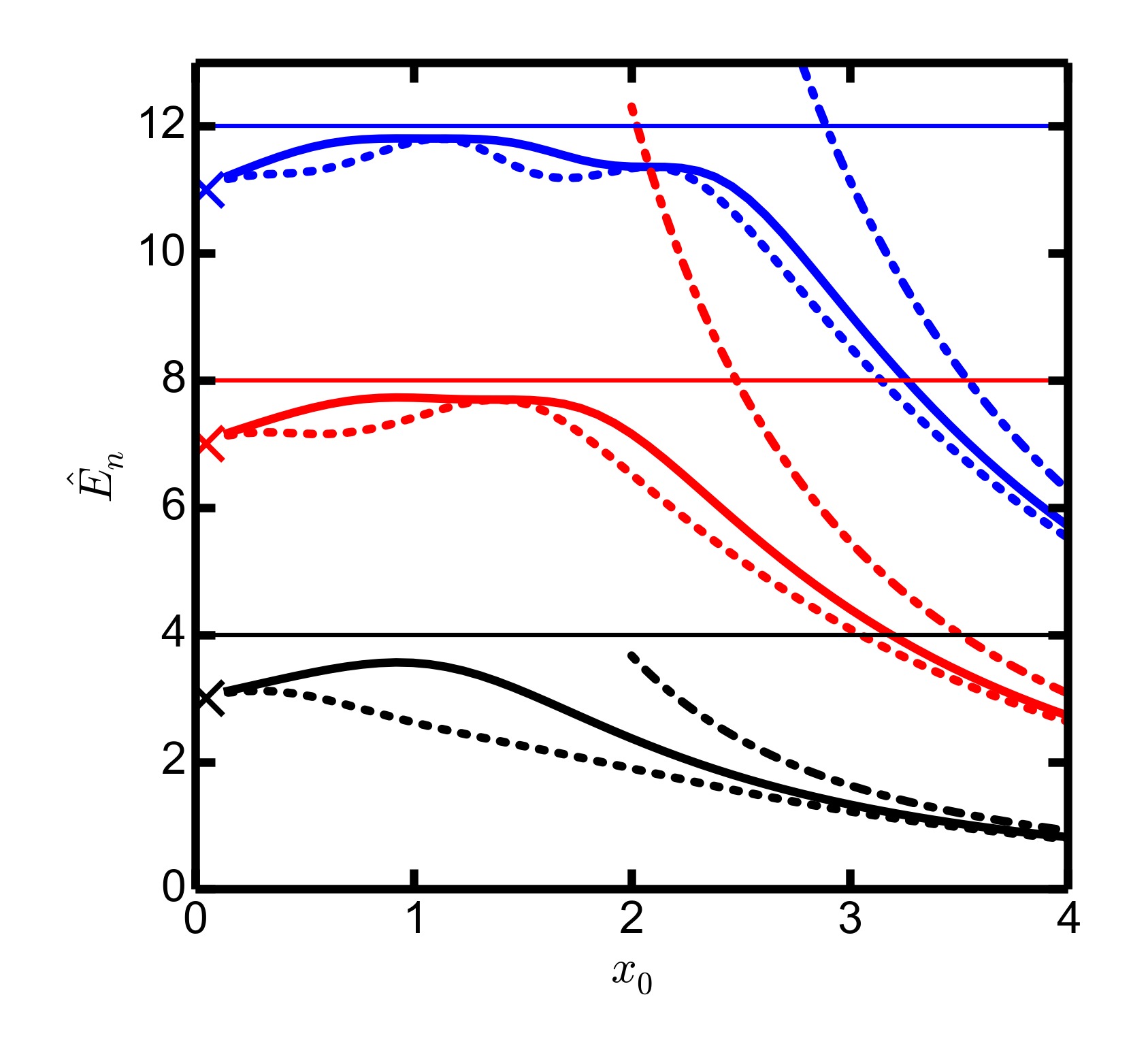
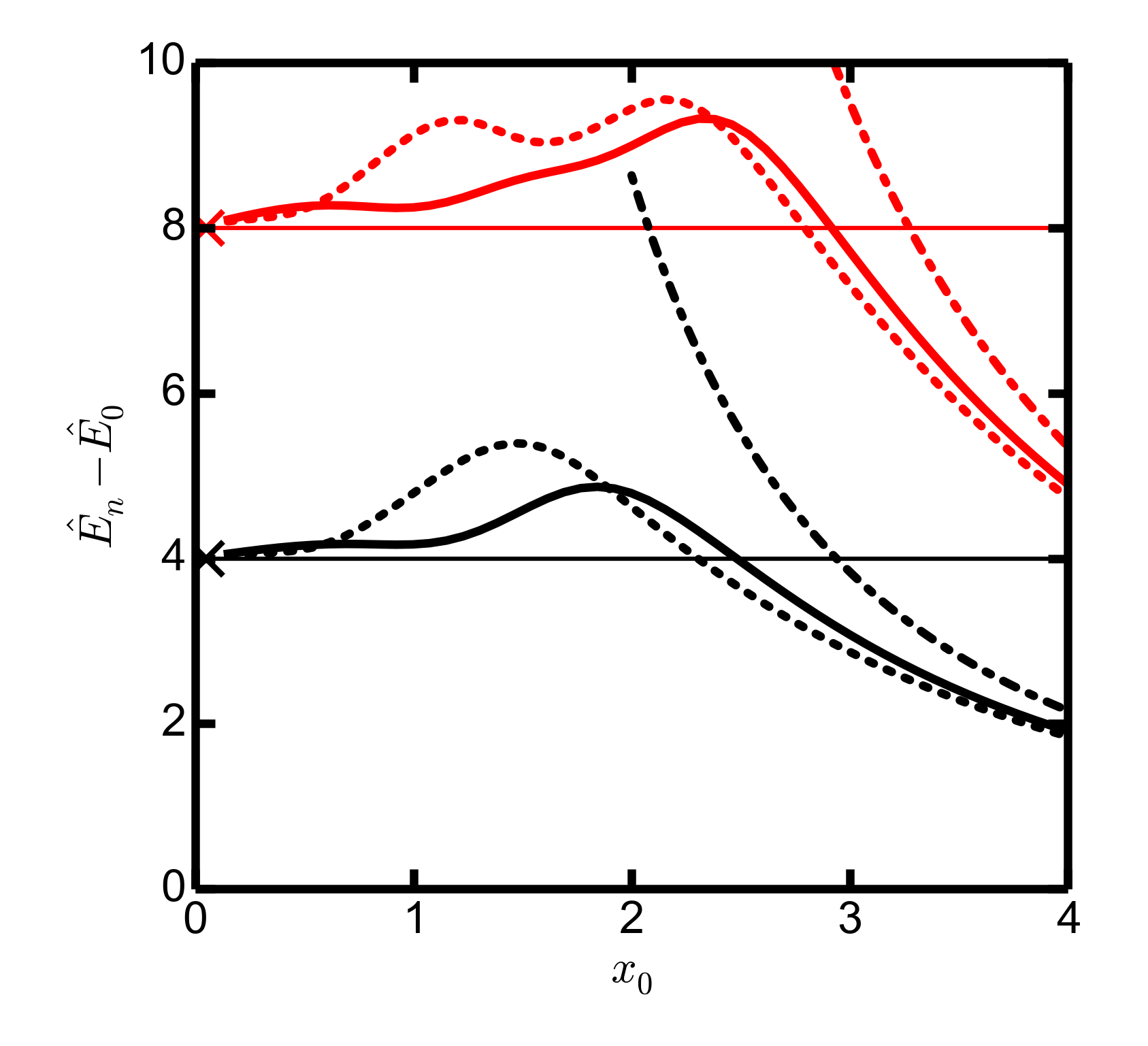
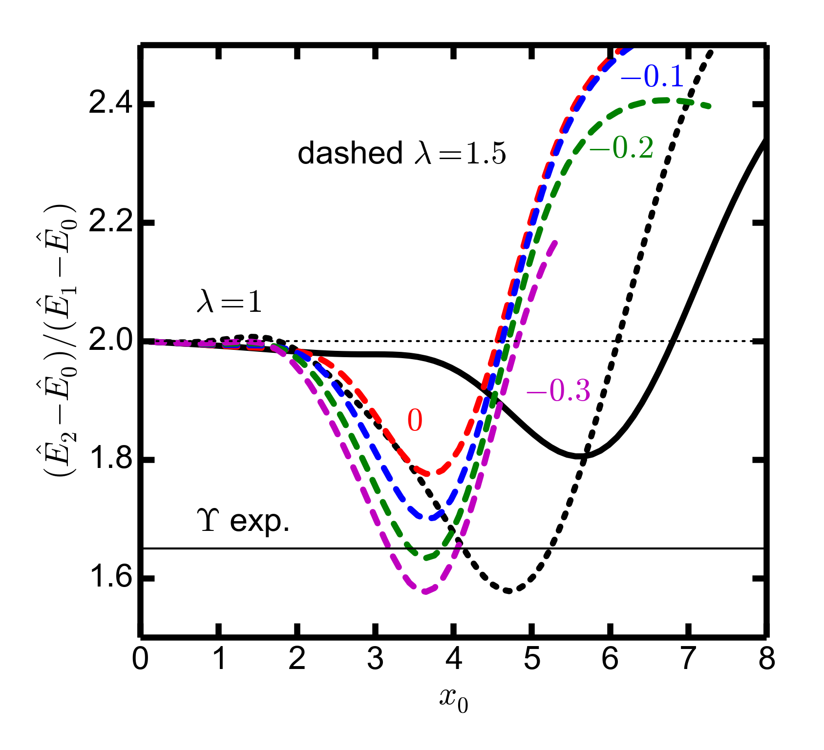
Figure 5: Survey on the properties of energy eigenvalues resulting from the Schrödinger-equivalent potential (26) under variation of the UV-IR matching point $x_{0}$ for the three options $\lambda=1$ (discontinuity at $x_{0}$), $\lambda\to 1$ (Dirac delta at $x_{0}$) and $\lambda>1$ ( box-like dip within $x_{0}\cdots\lambda x_{0}$). Left panel: The first energy eigenvalues $\hat{E}_{n}=L^{2}m_{n}^{2}$ for $\lambda=1$ (solid curves) and $\lambda\to 1$, $\tilde{U}_{0}=\Delta/(\lambda-1)$, $\Delta=-0.5L^{-2}$ (dotted curves). In addition, the crosses at $x_{0}=0$ are for the half-side harmonic oscillator, and the dashed curves at $x_{0}>2$ depict results of the r.h.s. hard wall at $x_{0}$. Thin horizontal lines are for the soft-wall model with $U_{0}^{SW}=U_{0}^{UV}+U_{0}^{IR}$. For $a=1$. Middle panel: As in left panel but for the level spacing, i.e. differences $\hat{E}_{n}-\hat{E}_{0}=L^{2}(m_{n}^{2}-m_{0}^{2})$. Right panel: Ratio $(\hat{E}_{2}-\hat{E}_{0})/(\hat{E}_{1}-\hat{E}_{0})=(m_{2}^{2}-m_{0}^{2})/(m_{1}^{2}-m_{0}^{2})$ for $\lambda=1$ (solid black curve) and $\lambda=1.5$ (dashed curves), displayed only for $\hat{E}_{n}>0$) with $L^{2}\tilde{U}_{0}=0$ (red), -0.1 (blue), -0.2 (green) and -0.3 (violet). The black dotted curve is as in the left and middle panels for the $\lambda\to 1$ model. The thin black horizontal line displays $(m_{\Upsilon(3S)}^{2}-m_{\Upsilon(1S)}^{2})/(m_{\Upsilon(2S)}^{2}-m_{\Upsilon(1S)}^{2})$ with experimental masses, while the thin dotted horizontal line depicts the maximum ratio value if one of the experimental masses is modified by $\pm 1$%. For $a=0.1$.

Despite the noticeable change of the energy eigenvalues $\hat{E}_{n}$ with changing parameter $x_{0}$ (see solid and dotted curves in the left panel), the level spacing is less influenced, see solid and dotted curves in the middle panel. The level spacing, given be differences of energy eigenvalues $\hat{E}_{n}-\hat{E}_{0}=L^{2}(m_{n}^{2}-m_{0}^{2})$ ($\approx 4a(n+1)$ for $x_{0}<1$, see middle panel), can be related to the $\Upsilon(1S,2S,3S)$ mass-squared differences $m_{n}^{2}-m_{0}^{2}$, 10.815 GeV² ($n=1$) and 17.623 GeV² ($n=2$), pointing either to $a\approx 0.1$ ($n=1$) or $a\approx 0.08$ ($n=2$), since $L^{-1}=5.148$ GeV. Clearly, the choice $\lambda=1$ only approximately accommodates the proper level spacing, as evidenced by two slightly different values of $a$.

In fact, the ratio $\frac{\hat{E}_{2}-\hat{E}_{0}}{\hat{E}_{1}-\hat{E}_{0}}$ (which is independent of $L^{2}$, $a$ and a shift by $b$) quantifies better the level spacing. It can be directly related to the experimental ratio $\frac{m_{\Upsilon(3S)}^{2}-m_{\Upsilon(1S)}^{2}}{m_{\Upsilon(2S)}^{2}-m_{\Upsilon(1S)}^{2}}$, see the thin black horizontal line in the right panel. The variation of the matching point $x_{0}$ in the $\lambda=1$ model (26) alone is not sufficient to meet exactly the experimental value, as pointed out above and depicted by the dashed black curve in the right panel. Tiny variations of one of the values of $m_{\Upsilon(nS)}$ on the 1% level induce changes of the ratio (see dotted horizontal line) which are comparable with the change caused by $x_{0}$ variation. The model (26) with $\lambda>1$ and suitable value of $\tilde{U}_{0}$, however, is capable to accommodate any of the wanted ratio value, see solid colored curves in the right panel for $a=0.1$. The choice $\lambda=1.5$ and various values of $L^{2}\tilde{U}_{0}$ represent examples of accomplishing the wanted fine-tuning. Analogously, the $\lambda\to 1$ model with suitable value of $\Delta$ is also appropriate (see black dotted curve).

The case $\lambda\to 1$ means replacing the $\tilde{U}_{0}$ dip in Eq. (26) for $x\in[x_{0},\lambda x_{0}]$ by a Dirac delta, $-\Delta\delta(x-x_{0})$. As pointed out above and in footnote 2, the solutions $y(\mbox{Eq.\leavevmode\nobreak\ (\ref{y_UV})})$ and $y(\mbox{Eq.\leavevmode\nobreak\ (\ref{y_IR})})$ and their derivatives must be matched at $x_{0}$ to yield

$$-\frac{1}{2x_{0}}\left[1-2\sqrt{\hat{E}}x_{0}\frac{J_{0}(\sqrt{\hat{E}}x_{0})}{J_{1}(\sqrt{\hat{E}}x_{0})}\right]-\frac{\sqrt{2a}}{2}\left[\sqrt{2a}x_{0}-2\frac{D_{\frac{\hat{E}+a}{2a}}(\sqrt{2a}x_{0})}{D_{\frac{\hat{E}-a}{2a}}(\sqrt{2a}x_{0})}\right]=\Delta$$ (IV)

for discrete energy eigenvalues $\hat{E}(x_{0},a,\Delta)$ to be numerated by $n$, see dotted curves in Fig. 5.