A meshfree arbitrary Lagrangian-Eulerian method for the BGK model of the Boltzmann equation with moving boundaries

Abstract

In this paper we present a novel technique for the simulation of moving boundaries and moving rigid bodies immersed in a rarefied gas using an Eulerian-Lagrangian formulation based on least square method. The rarefied gas is simulated by solving the Bhatnagar-Gross-Krook (BGK) model for the Boltzmann equation of rarefied gas dynamics. The BGK model is solved by an Arbitrary Lagrangian-Eulerian (ALE) method, where grid-points/particles are moved with the mean velocity of the gas. The computational domain for the rarefied gas changes with time due to the motion of the boundaries. To allow a simpler handling of the interface motion we have used a meshfree method based on a least-square approximation for the reconstruction procedures required for the scheme. We have considered a one way, as well as a two-way coupling of boundaries/rigid bodies and gas flow. The numerical results are compared with analytical as well as with Direct Simulation Monte Carlo (DSMC) solutions of the Boltzmann equation. Convergence studies are performed for one-dimensional and two-dimensional test-cases. Several further test problems and applications illustrate the versatility of the approach.

MSC2020: 65C05, 65M99, 70E99, 76P05, 76T20
Keywords: rarefied gas, kinetic equation, BGK model, meshfree method, ALE method, semi-implicit method, least squares method, gas rigid body interactions

1 Introduction

In recent years moving boundary problems for rarefied gas dynamics have been extensively investigated in the connection with Micro-Electro-Mechanical-Systems (MEMS), see [5, 12, 13, 16, 19, 23, 27, 28, 33, 29, 30]. In micro scale geometries the mean free path is often of the order or larger than the characteristic length of the geometry, even at standard condition of temperature and pressure, thus requiring the physical system to be described by kinetic equations. Usually, these flows have low Mach numbers, therefore, stochastic methods like DSMC are not the optimal choice, since statistical noise dominates the flow quantities. Moreover, when one considers moving rigid body, the gas domain will change in time and one has to encounter unsteady flow problems, so that averages over long runs cannot be taken. Instead, one has to perform many independent runs in order to get smooth solutions. Although some attempts have been made to reduce the statistical noise of DSMC type methods, see, for example, [11], or to adopt efficient solvers for the Boltzmann equation, such as those based on the Fourier-spectral method (see for example the review paper [14]), many works rather employ deterministic approaches for simplified models of the Boltzmann equation, like the Bhatnagar-Gross-Krook (BGK) model, see [12, 23, 29, 34, 35]. In the above mentioned works either Finite-Difference schemes or Semi-Lagrangian methods are used to solve the moving boundary problems, see [12] for an overview of methods used for the BGK equation. Since the rigid body moves in time, classical interpolation procedures near the rigid body become complicated and possibly inaccurate because of the arbitrary intersection of cells by the rigid body. Thus, a Cartesian cut cell method has been introduced in [13] to handle the moving object in the rarefied gas. A different technique has been used in [10], where the authors have used ghost point methods in a finite difference framework to treat moving boundaries. For immersed boundary type approaches applied to kinetic equations to simulate the fluid-rigid body interactions see [3, 12, 35].

In the present paper we use a deterministic Arbitrary Lagrangian-Eulerian approach for the BGK model. First and second order versions of the scheme and associated upwinding procedure are described and numerically tested. This approach, based on moving grid points, is simple, well suited and very efficient for the treatment of problems with moving boundaries. While the interior grid points are moved with the mean velocity of the gas, the moving boundaries are as well approximated by a discrete set of boundary points moving with the boundaries. This leads to a very flexible scheme also suited for complicated geometries and flows.

The paper is organised as follows. In section 2 we present the BGK model for the Boltzmann equation, the Newton-Euler equations for rigid body motions and the Chu reduction procedure. In section 3 we introduce the numerical scheme for the BGK model, in particular the spatial and temporal discretization with first and second order accuracy. Section 4 illustrates various numerical results in one and two space dimensions including a convergence study in 1D and 2D and comparisons with DSMC results. Finally, in section 5 some conclusions and an outlook are presented.

2 The BGK model for rarefied gas dynamics

We consider the BGK model of the Boltzmann equation for rarefied gas dynamics, where the collision term is modeled by a relaxation of the distribution function $f(t,x,v)$ to the Maxwellian equilibrium distribution. The evolution equation for the distribution function $f(t,x,v)$ is given by the following initial boundary value problem

$$\frac{\partial f}{\partial t}+v\cdot\nabla_{x}f=\frac{1}{\tau}(M-f)$$ (1)

with $t\geq 0,x\in\Omega\subset\mathbb{R}^{d_{x}},(d_{x}=1,2,3),\;v\in\mathbb{R}^{d_{v}},(d_{v}=1,2,3)$ and initial condition $f(0,x,v)=f_{0}(x,v)$. Additionally, suitable boundary conditions are described, see the next section. Here $\tau$ is the relaxation time, which may depend on local density and temperature, and $M$ is the local Maxwellian given by

$$M=\frac{\rho}{(2\pi RT)^{d_{v}/2}}\exp\left(\frac{|v-U|^{2}}{2RT}\right),$$ (2)

where the parameters $\rho(x,t)\in\mathbb{R},U(x,t)\in\mathbb{R}^{d_{v}},T(x,t)\in\mathbb{R}$ are the macroscopic quantities mass density, mean velocity and temperature, respectively. $R$ is the universal gas constant divided by the molecular mass of the gas. $\rho,U,T$ are computed from $f$ as follows. Let the moments of $f$ be defined by

$$(\rho,\rho U,E)=\int_{\mathbb{R}^{3}}\phi(v)f(t,x,v)dv.$$ (3)

where ${\phi}(v)=\left(1,v,\frac{|v|^{2}}{2}\right)$ denotes the vector of collision invariants. $E$ is the total energy density which is related to the temperature through the internal energy

$$e(t,{x})=\frac{3}{2}RT,\quad\quad\rho e=E-\frac{1}{2}\rho|U|^{2}.$$ (4)

The relaxation time $\tau=\tau(x,t)$ and the mean free path $\lambda$ are related according to [9]

$$\tau=\frac{4\lambda}{\pi\bar{C}},$$ (5)

where $\bar{C}=\sqrt{{8RT}/{\pi}}$ and the mean free path $\lambda$ is given by

$$\lambda=\frac{k_{B}}{\sqrt{2}\pi\rho Rd^{2}},$$ (6)

where $k_{B}$ is the Boltzmann constant and $d$ is the diameter of the gas molecules.

2.1 Newton-Euler equations for rigid body motion

The motion of a rigid body $S\subset\mathbb{R}^{d_{x}}$ is given by the Newton-Euler equations, compare [34],

$$M\frac{d{V}}{dt}={\mathcal{{F}}},\;\;[I]\cdot\frac{d{\omega}}{dt}+{{\omega}}\times({[I]\cdot}{{\omega}})={\mathcal{{T}}},$$ (7)

where $M$ is the total mass of the body with center of mass ${X}_{c}$, ${V}$ is the velocity of the center of mass ${X}_{c}$ and ${\omega}$ is the angular velocity of the rigid body. $\mathcal{{F}}$ is the translation force, $\mathcal{{T}}$ is the torque and $[I]$ is the moment of inertia. The center of mass of the rigid body is obtained by

$$\frac{d{X}_{c}}{dt}={V}.$$ (8)

Finally, the velocity of a point on the surface of the rigid body is given by ${{U}_{w}}={{V}}+{{\omega}}\times({{x}}-{{X}_{c}}),~{}{{x}}\in\partial S$.

The force $\mathcal{{F}}$ and torque ${\mathcal{{T}}}$, that the gas exerts on the rigid body, are computed according to

$$\mathcal{{F}}=\int_{\partial S}(-\varphi\cdot{{n}}_{s})dA,\;\;\mathcal{{T}}=\int_{\partial S}({x}-{X}_{c})\times(-\varphi\cdot{{n}}_{s})dA,$$ (9)

where $\varphi\in\mathbb{R}^{d_{x}\times d_{x}}$ is the stress tensor and is given by

$$\varphi=\int_{\mathbb{R}^{3}}({v}-{U}_{w})\otimes({v}-{U}_{w})f(t,{x},{v})d{v}.$$ (10)

2.2 Chu-reduction

In one and two physical space dimensions $d_{x}=1,2$ one might consider mathematically a one or two dimensional velocity space $d_{v}=1,2$, respectively. However, it is physically correct to consider in these situations still three velocity dimensions. To resolve the three-dimensional velocity space numerically requires unnecessary memory and computational time. In these cases, for the BGK model, the 3D velocity space can be reduced as suggested by Chu [6]. This reduction yields a considerable savings in memory allocation and computational time. For example, in a physically one-dimensional situation, in which all variables depend on $x\in\mathbb{R}$ and $t$ (slab geometry), the velocity space is reduced from three dimensions to one dimension defining the following reduced distributions [18]. Considering $v=(v_{1},v_{2},v_{3})\in\mathbb{R}^{3}$ we define

$$g_{\rm 1}(t,x,v_{1})=\int_{\mathbb{R}^{2}}f(t,x,v_{1},v_{2},v_{3})dv_{2}dv_{3},\quad g_{\rm 2}(t,x,v_{1})=\int_{\mathbb{R}^{2}}(v_{2}^{2}+v_{3}^{2})f(t,x,v_{1},v_{2},v_{3})dv_{2}dv_{3}.$$ (11)

Multiplying (1) by $1$ and $v_{2}^{2}+v_{2}^{2}$ and integrating with respect to $(v_{2},v_{3})\in\mathbb{R}^{2}$, we obtain the following system of two equations

$$\frac{\partial g_{1}}{\partial t}+v\frac{\partial g_{1}}{\partial x}=\frac{1}{\tau}(G_{1}-g_{1}),\quad\frac{\partial g_{2}}{\partial t}+v\frac{\partial g_{2}}{\partial x}=\frac{1}{\tau}(G_{2}-g_{2}),$$ (12)

where we denoted $v_{1}$ by $v$, and

$$G_{1}=\int_{\mathbb{R}^{2}}Mdv_{2}dv_{3}=\frac{\rho}{\sqrt{2RT}}\exp\left({-\frac{(v-U)^{2}}{2RT}}\right),\quad G_{2}=\int_{\mathbb{R}^{2}}(v_{2}^{2}+v_{3}^{2})Mdv_{2}dv_{3}=(2RT)G_{1}.$$ (13)

Assuming the initial condition is a local equilibrium, the initial distributions are defined via the parameters $(\rho_{0},U_{0},T_{0})\in\mathbb{R}^{3}$ and are given as

$$g_{1}(0,x,v)=\frac{\rho_{0}}{\sqrt{2RT_{0}}}\exp\left({-\frac{(v-U_{0})^{2}}{2RT_{0}}}\right),\quad g_{2}(0,x,v)=(2RT_{0})g_{1}(0,x,v).$$ (14)

The macroscopic quantities are given through the reduced distributions as

$$\rho=\int_{\mathbb{R}}g_{1}dv,\;\rho U=\int_{\mathbb{R}}vg_{1}dv,\;3\rho RT=\int_{\mathbb{R}}(v-U)^{2}g_{1}dv+\int_{\mathbb{R}}g_{2}dv.$$ (15)

Similarly, in two spatial dimensions $x\in\mathbb{R}^{2}$, the reduction from a three dimensional to a two dimensional velocity space is obtained by multiplying the BGK model (1) by $1$ and $v_{3}^{2}$ and integrating wrt $dv_{3}$ over $\mathbb{R}$. The reduced equations are two-dimensional versions of (12) with $v=(v_{1},v_{2})\in\mathbb{R}^{2}$, but the reduced Maxwellians $G_{1}$ and $G_{2}$ are given as

$$G_{1}=\frac{\rho}{2RT}\exp\left({-\frac{|v-U|^{2}}{2RT}}\right),\quad G_{2}=(RT)G_{1}$$ (16)

with $U=(U_{1},U_{2})\in\mathbb{R}^{2}$. The distribution functions are

$$g_{1}(t,x,v_{1},v_{2})=\int_{\mathbb{R}}f(t,x,v_{1},v_{2},v_{3})dv_{3},\quad g_{2}(t,x,v_{1},v_{2})=\int_{\mathbb{R}}v_{3}^{2}f(t,x,v_{1},v_{2},v_{3})dv_{3}.$$

3 Numerical schemes

We solve the original equation (1) and the reduced system of equations (12) by the ALE method described below. We use a time splitting, where the advection step is solved explicitly and the relaxation part is solved implicitly. Using a discrete velocity approximation of the distribution function (see Section 3.3) the information is stored on grid points in physical space moving with the mean velocity $U$ of the gas. The spatial derivatives of the distribution function at an arbitrary particle position are approximated using values at the point-cloud surrounding the particle and a weighted least squares method.

In the following. we present first and second order schemes in time as well as in space.

3.1 ALE formulation

We consider original and reduced model.

3.1.1 ALE formulation for the original model

We rewrite the equations (1) in Lagrangian form as

$$\frac{dx}{dt} = U$$ (17)

$$\frac{df}{dt} = -(v-U)\cdot\nabla_{x}f+\frac{1}{\tau}(M-f)$$ (18)

where ${d}/{dt}={\partial}/{\partial t}+U\cdot\nabla_{x}$. The first equation describes motion with the macroscopic mean velocity $U$ of the gas determined by (15). The second equation includes the remaining advection with the difference between microscopic and macroscopic velocity.

3.1.2 ALE for reduced model

In this case the equations (11) are reformulated in Lagrangian form as

$$\frac{dx}{dt} = U$$ (19)

$$\frac{dg_{1}}{dt} = -(v-U)\cdot\nabla_{x}g_{1}+\frac{1}{\tau}(G_{1}-g_{1})$$ (20)

$$\frac{dg_{2}}{dt} = -(v-U)\cdot\nabla_{x}g_{2}+\frac{1}{\tau}(G_{2}-g_{2}).$$ (21)

3.2 Time discretization

3.2.1 First order time splitting scheme for the original model

Time is discretized as $t^{n}=n\Delta t,n=0,1,\cdots,N_{t}$. We denote the numerical approximation of $f$ at $t_{n}$ by $f^{n}=f(t^{n},x,v)$. We use a time splitting scheme for equation (18), where the advection term is solved explicitly and the collision term is solved implicitly. In the first step of the splitting scheme we obtain the intermediate distribution $\tilde{f}^{n}$ by solving

$$\tilde{f}^{n} = f^{n}-\Delta t(v-U^{n})\cdot\nabla_{x}f^{n}.$$ (22)

In the second step we obtain the new distribution by solving

$$f^{n+1} = \tilde{f}^{n}+\frac{\Delta t}{\tau}(M^{n+1}-f^{n+1})$$ (23)

and the new positions of the grids are updated by

$$x^{n+1}=x^{n}+\Delta tU^{n}.$$ (24)

In the first step, we have to approximate the spatial derivatives of $f$ at every grid point. This is described in the following section.

Following [17, 18, 37] we obtain $f^{n+1}$ in the second step by first determining the parameters $\rho^{n+1},U^{n+1}$ and $T^{n+1}$ for $M^{n+1}$. Multiplying (23) by $1$, $v$ and $(v-U)^{2}$ and integrating over velocity space, we get

$$\rho^{n+1}=\int_{\mathbb{R}}\tilde{f}^{n}dv,\quad(\rho U)^{n+1}=\int_{\mathbb{R}}v\tilde{f}^{n}dv,\quad 3\rho RT^{n+1}=\int_{\mathbb{R}^{3}}|v-U|^{2}\tilde{f}^{n}dv$$ (25)

where we have used the conservation of mass, momentum and energy of the original BGK model.

Now, the parameters $\rho^{n+1},U^{n+1}$ and $T^{n+1}$ of $M^{n+1}$ are given in terms of $\tilde{f}$ from (25) . Hence the implicit step (23) can be explicitly solved as

$$f^{n+1}=\frac{\tau\tilde{f}^{n}+\Delta tM^{n+1}}{\tau+\Delta t}.$$ (26)

3.2.2 Second order splitting scheme for the original model (ARS(2,2,2))

For the second order splitting scheme we use the stiffly accurate ARS(2,2,2) scheme, [4], and compare the results with a slightly simpler scheme ARS(2,2,1). The Butcher tabueau of both schemes are reported below, in the usual form expressed in Table 1

$c$	$A$
	$b^{\intercal}$

$\tilde{c}$	$\tilde{A}$
	$\tilde{b}^{\intercal}$

Table 1: Classical form of the double Butcher tableau of an IMEX scheme: matrix $A$ and vectors $b$ and $c$ are relative to the implicit scheme, while $\tilde{A}$, $\tilde{b}$, $\tilde{c}$ denote the RK coefficients of the implicit scheme.

$$\quad\quad\begin{array}[]{ c | ccc }0&0&0&0\\ \beta&0&\beta&0\\ 1&0&1-\beta&\beta\\ \hline\cr&0&1-\beta&\beta\\ \end{array}\quad\begin{array}[]{ c | ccc }0&0&0&0\\ \beta&\beta&0&0\\ 1&\beta-1&2-\beta&0\\ \hline\cr&\beta-1&2-\beta&0\\ \end{array}\quad\quad\quad\begin{array}[]{ c | ccc }0&0&0&0\\ 1/2&0&1/2&0\\ 1&0&0&1\\ \hline\cr&0&0&1\\ \end{array}\quad\begin{array}[]{ c | ccc }0&0&0&0\\ 1/2&1/2&0&0\\ 1&0&1&0\\ \hline\cr&0&1&0\\ \end{array}$$

Table 2: Tableau of ARS(2,2,2) scheme (left) and of ARS(2,2,1) scheme (right). $\beta=1-1/\sqrt{2}$.

For equation (17-18) this leads to

Step 1:

$$x^{n+\frac{1}{2}} = x^{n}+\beta\Delta tU^{n}.$$ (27)

$$\tilde{f}^{n+\frac{1}{2}} = f^{n}-\beta\Delta t(v-U^{n})\cdot\nabla_{x}f^{n}.$$ (28)

The intermediate distributions $f^{n+\frac{1}{2}}$ are then obtained by solving

$$f^{n+\frac{1}{2}} = \tilde{f}^{n+\frac{1}{2}}+\beta\frac{\Delta t}{\tau}(M^{n+\frac{1}{2}}-f^{n+\frac{1}{2}})$$

or

$$f^{n+\frac{1}{2}}=\frac{\tau\tilde{f}^{n+\frac{1}{2}}+\beta\Delta tM^{n+\frac{1}{2}}}{\tau+\beta\Delta t}.$$ (29)

Step 2:

$$x^{n+1} = x^{n}+\Delta t((\beta-1)U^{n}+(2-\beta)U^{n+\frac{1}{2}}).$$ (30)

$$\tilde{f}^{n+1} = f^{n}-(2-\beta)\Delta t(v-U^{n+\frac{1}{2}})\cdot\nabla_{x}f^{n+\frac{1}{2}}$$

$$-(\beta-1)\Delta t(v-U^{n})\cdot\nabla_{x}f^{n}$$

$$+(1-\beta)\frac{\Delta t}{\tau}(M^{n+\frac{1}{2}}-f^{n+\frac{1}{2}}).$$

The new distributions are obtained by solving

$$f^{n+1} = \tilde{f}^{n+1}+\beta\frac{\Delta t}{\tau}(M^{n+1}-f^{n+1}).$$

or

$$f^{n+1}=\frac{\tau\tilde{f}^{n+1}+\beta\Delta tM^{n+1}}{\tau+\beta\Delta t}.$$ (32)

with $\beta=1-1/{\sqrt{2}}$. We note that the implicit computations of $M^{n+\frac{1}{2}}$ and of $M^{n}$ are similar to the implicit computation of $M^{n+1}$ in the first order scheme as described above.

3.2.3 Partial second order time splitting scheme for the original model ARS(2,2,1))

For later use we also describe a simplified scheme with an explicit second order solution of the advection equation and an implicit first order solution of the collision term. For the second order scheme we use a two step Runge-Kutta scheme. For equation (17-18) the scheme is given by
Step 1:

$$x^{n+\frac{1}{2}} = x^{n}+\frac{\Delta t}{2}U^{n}.$$ (33)

$$\tilde{f}^{n+\frac{1}{2}} = f^{n}-\frac{\Delta t}{2}(v-U^{n})\cdot\nabla_{x}f^{n}.$$ (34)

The intermediate distributions $f^{n+\frac{1}{2}}$ are then obtained by solving

$$f^{n+\frac{1}{2}} = \tilde{f}^{n+\frac{1}{2}}+\frac{1}{2}\frac{\Delta t}{\tau}(M^{n+\frac{1}{2}}-f^{n+\frac{1}{2}})$$

i.e.

$$f^{n+\frac{1}{2}}=\frac{2\tau\tilde{f}^{n+\frac{1}{2}}+\Delta tM^{n+\frac{1}{2}}}{2\tau+\Delta t}.$$ (35)

Step 2:

$$x^{n+1} = x^{n}+\Delta tU^{n+\frac{1}{2}}.$$ (36)

$$\tilde{f}^{n+1} = f^{n}-\Delta t(v-U^{n+\frac{1}{2}})\cdot\nabla_{x}f^{n+\frac{1}{2}}.$$ (37)

The new distributions are obtained by solving

$$f^{n+1} = \tilde{f}^{n+1}+\frac{\Delta t}{\tau}(M^{n+1}-f^{n+1}).$$ (38)

or

$$f^{n+1}=\frac{\tau\tilde{f}^{n+1}+\Delta tM^{n+1}}{\tau+\Delta t}.$$ (39)

Remark 1.

Note that this scheme is not the Midpoint rule, which is A-stable, but not L-stable. It is not second order, but it is L-stable, therefore it can be adopted with arbitrarily small values of the relaxation time $\tau$. However, the scheme is simpler and less costly than the ARS scheme and in the examples considered here, we obtain numerically second order of convergence.

3.2.4 Time splitting scheme for the reduced model

We use again a time splitting scheme. For the first order scheme with one-dimensional physical space $x\in\mathbb{R}$, we proceed as follows. In the first step we obtain the intermediate distributions $\tilde{g}^{n}_{1}$ and $\tilde{g}^{n}_{2}$ by solving for $v\in\mathbb{R}$ and $U\in\mathbb{R}$

$$\tilde{g}_{1}^{n}=g_{1}^{n}-\Delta t(v-U^{n})\partial_{x}g_{1}^{n}\quad\tilde{g}_{2}^{n}=g_{2}^{n}-\Delta t(v-U^{n})\partial_{x}g_{2}^{n}.$$

In the second step we obtain the new distributions by solving

$$g_{1}^{n+1} = \tilde{g}_{1}^{n}+\frac{\Delta t}{\tau}(G_{1}^{n+1}-g_{1}^{n+1})$$ (40)

$$g_{2}^{n+1} = \tilde{g}_{2}^{n}+\frac{\Delta t}{\tau}(G_{2}^{n+1}-g_{2}^{n+1})$$ (41)

and the new positions of the grids are updated by

$$x^{n+1}=x^{n}+\Delta tU^{n}.$$ (42)

For the second step we have to determine first the parameters $\rho^{n+1},U^{n+1}$ and $T^{n+1}$ for $G_{1}^{n+1}$ and $G_{2}^{n+1}$. Multiplying (40) by $1$ and $v$ and integrating with respect to $v$ over $\mathbb{R}$ we get

$$\rho^{n+1}=\int_{\mathbb{R}}\tilde{g}_{1}^{n}dv,\quad(\rho U)^{n+1}=\int_{\mathbb{R}}v\tilde{g}_{1}^{n}dv,$$ (43)

where we have used the conservation of mass and momentum of the original BGK model. In order to compute $T^{n+1}$ we note that the following identity is valid

$$\int_{\mathbb{R}}(v-U)^{2}(G_{1}-g_{1})dv+\int_{\mathbb{R}}(G_{2}-g_{2})dv=0.$$ (44)

Multiplying the equation (40) by $(v-U)^{2}$ and integrate with respect to $v$ over $\mathbb{R}$ we get

$$\int_{\mathbb{R}}(v-U)^{2}g_{1}^{n+1}dv=\int_{\mathbb{R}}(v-U)^{2}\tilde{g}_{1}^{n}dv+\frac{\Delta t}{\tau}\int_{\mathbb{R}}(v-U)^{2}(G_{1}^{n+1}-g_{1}^{n+1})dv.$$ (45)

Next, integrate both sides of 41) with respect to $v$ over $\mathbb{R}$ we get

$$\int_{\mathbb{R}}g_{2}^{n+1}dv=\int_{\mathbb{R}}\tilde{g}_{2}^{n}dv+\frac{\Delta t}{\tau}\int_{\mathbb{R}}(G_{2}^{n+1}-g_{2}^{n+1})dv.$$ (46)

Adding (45) and (46) and making use of the identity (44) we get

$$3\rho^{n+1}RT^{n+1}=\int_{\mathbb{R}}(v-U)^{2}\tilde{g}_{1}^{n}dv+\int_{\mathbb{R}}\tilde{g}_{2}^{n}dv.$$ (47)

Now, the parameters $\rho^{n+1},U^{n+1}$ and $T^{n+1}$ of $G_{1}^{n+1}$ and $G_{2}^{n+1}$ are given in terms of $\tilde{g}_{1}^{n}$ and $\tilde{g}_{2}^{n}$ from (43) and (47). Hence the implicit steps (40) and (41) can be rewritten as

$$g_{1}^{n+1}=\frac{\tau\tilde{g}_{1}^{n}+\Delta tG_{1}^{n+1}}{\tau+\Delta t}$$ (48)

$$g_{2}^{n+1}=\frac{\tau\tilde{g}_{2}^{n}+\Delta tG_{2}^{n+1}}{\tau+\Delta t}.$$ (49)

The second order time splitting for the reduced model follows the lines of the second order splitting procedure for the original model.

3.3 Velocity discretization

For the sake of simplicity we consider a one-dimensional velocity domain. Consider $N_{v}+1$ velocity grid points and a uniform velocity grid of size $\Delta v=2v_{\rm max}/N_{v}$ We assume that the distribution function is negligible for $|v|>v_{\rm max}$ and discretize $[-v_{\rm max},v_{\rm max}]$. That means for each velocity direction we have the discretization points $v_{j}=-v_{\rm max}+(j-1)\Delta{v},j=1,\ldots,N_{v}+1$. Note that the performance of the method could be improved by using a grid adapted to the mean velocity $U$, see, for example, [12].

3.4 Spatial discretization

We discuss the spatial discretization and upwinding procedures for first and second order schemes.

3.4.1 Approximation of spatial derivatives

In the above numerical schemes an approximation of the spatial derivatives of $g_{1}$ and $g_{2}$ is required. In this subsection, we describe a least squares approximation of the derivatives on the moving point cloud based on so called generalized finite differences, see [21, 26] and references there in. A stabilizing procedure using upwinding and a WENO type discretization for the higher order schemes will be described in the following.

For the sake of simplicity we consider a one-dimensional spatial domain $\Omega$. We first approximate the boundary of the domain by a set of discrete points called boundary particles. In the second step we approximate the interior of the computational domain using another set of interior points or interior particles. The sum of boundary and interior points gives the total number of points. We note that the boundary conditions are applied on the boundary points. The boundary points move together with the boundaries. The initial generation of grid points can be regular as well as arbitrary. When the points move they can form a cluster or can scatter away from each other. In these cases, either some grid points have to be removed or new grid points have to be added. We will describe this particle management in the next subsection.

Let ${x}_{i}\in\Omega,i=1,\ldots,N_{x}$, where $N_{x}$ is the total number of grid points with initial average spacing $\Delta x$. Let $f(x)$ be a scalar function and $f_{i}$ its discrete values in $x_{i}$. Our main task is to approximate the spatial derivatives of $f_{i}$ at an arbitrary position $x_{i}$ from its neighboring particles. We call $x_{i}$ a central point. We sort the neighboring points into different catagories, left, right and central neighbor. Note that the point $x_{i}$ is itself its neighbor in all sets of neighboring particles. We restrict to neighboring points within a radius $h$ in such a way that we have at least a minimum number of neighbors. $h$ is usually chosen in relation to $\Delta x$, compare [31]. For a first order approximation one can choose smaller values of $h$ than for a higher order approximation. In order to guarantee a better accuracy we associate a weight function depending on the distance of the central point and its neighbors. Let $P(x)=x_{k},k=1,\ldots,m$ be the set of $m$ neighbor points of $x=x_{i}$ inside the radius $h$. There are several choices of weight functions [25]. We choose a Gaussian weight function [31, 32]

$$w({x}_{k}-x;h)=\left\{\begin{array}[]{l}\exp\left(-\alpha\frac{(x_{k}-x)^{2}}{h^{2}}\right),\\ 0,\qquad\qquad\mbox{else},\end{array}\right.$$

with $\alpha$ a user defined positive constant. In our computation, we have chosen $\alpha=6$.

In order to approximate the derivatives we consider a second order Taylor expansion of $f(x_{k})$ around $x$

$$f(x_{k})=f(x)+(x_{k}-x)\cdot\partial_{x}f(x)+(x_{k}-x)^{T}\partial_{xx}f(x)(x_{k}-x)+e_{k},$$ (52)

for $k=1,\ldots,m$, where $e_{k}$ is the error in the Taylor’s expansion. The unknown $a=[\frac{\partial f}{\partial x}(x),\frac{\partial^{2}f}{\partial x^{2}}(x)]^{T}$ is now computed by minimizing the error $e_{k}$ for $k=1,\ldots,m$. The system of equations can be re-written in vector form as

$${e}={b}-Da,$$ (53)

where ${e}=[e_{1},\ldots,e_{m}]^{T}$, $b=[f_{1}-f(x),\ldots,f_{m}-f(x)]^{T}$ and

$$D=\left(\begin{array}[]{cc}dx_{1}&~{}\frac{1}{2}dx^{2}_{1}\\ \vdots&\vdots\\ dx_{m}&~{}\frac{1}{2}dx^{2}_{m}\end{array}\right)$$ (57)

with $dx_{k}=x_{k}-x$.

Imposing $e=0$ in (53) results in an overdetermined linear stems of algebraic equations, which in general has no solution. The unknown $a$ is therefore obtained from the weighted least squares method by minimizing the quadratic form

$$J=\sum_{k=1}^{m}w_{k}e_{k}^{2}=(Da-{b})^{T}W(Da-{b}),$$ (58)

where $W=\mathrm{d}iag(w_{1},\ldots,w_{m})$. The minimization of $J$ formally yields

$$a=(D^{T}WD)^{-1}(D^{T}W){b}.$$ (59)

3.4.2 First order upwind scheme

We describe the procedure for simplicity only for one-dimensional physical space. We compute the partial derivatives of $g_{1}$ and $g_{2}$ in the following way. If $v-U>0$, we compute the derivatives at $x_{i}$ from the set of left neighbors $P_{L}(x_{i})$ lying within the radius $h$. Similarly, for $v-U<0$ we use the set of right neighbors $P_{R}(x_{i})$ lying within the radius $h$. Then we use the Taylor expansion (52) to first order and compute the derivatives in the corresponding set of neighboring points.

3.4.3 Second order WENO-type procedure

When we apply a second order Taylor expansion, the scheme becomes unstable if the solution develops discontinuities. In this case we use the WENO idea in order to obtain higher order derivatives. We refer to [1, 2, 38] for similar approaches for SPH-type particle methods. For the sake of simplicity, we consider the one dimensional case to present our simplified WENO procedure. Let $P_{L}(x_{i}),P_{R}(x_{i})$ and $P_{C}(x_{i})$ be the sets of left, right and central neighbor points, see Fig. 1. Note that $P_{C}(x_{i})=P_{L}(x_{i})\cup P_{R}(x_{i})$.

Fig. 1: Central, left and right neighbor points.

Considering the Taylor expansions (52) and applying the least squares method, we obtain the derivatives

$${f_{x}}_{L},{f_{xx}}_{L},{f_{x}}_{R},{f_{xx}}_{R},{f_{x}}_{C},{f_{xx}}_{C}$$

using left, central and right neighbors, respectively. The desired first order derivative is obtained by the weighted sum

$$f_{x} = \omega_{L}{f_{x}}_{L}+\omega_{C}{f_{x}}_{C}+\omega_{R}{f_{x}}_{R},$$ (60)

where the weights are defined by

$$\omega_{k}=\frac{\beta_{k}}{\beta_{L}+\beta_{C}+\beta_{R}},\quad k=L,C,R$$ (61)

with

$$\beta_{k}=\frac{C_{k}}{({f_{x}}_{k}^{2}\Delta x^{2}+{f_{xx}}_{k}^{2}\Delta x^{4}+\epsilon)^{2}},\quad k=L,C,R$$ (62)

where $\epsilon=10^{-6}$ and $\Delta x$ is the initial spacing of particles. This is combined with the following choice of the coefficients $C_{k}$ depending on the sign of $v-U$. If $v-U>0$ the values are

$$C_{L}=0.5,C_{C}=0.5,C_{R}=0$$

and otherwise

$$C_{L}=0,C_{C}=0.5,C_{R}=0.5.$$

In 2D we proceed in an analogous way. Here the derivatives $f_{x}$ and $f_{y}$ are required. They are obtained by determining the sets of points in the left (L) and right (R) half plane for the determination of $f_{x}$ and the sets in the top (T) and bottom (B) half plane for the determination of $f_{y}$, see Fig. 2.

Fig. 2: Subdivision of the neighbors of a given point into subsets, used for the computation of the polynomials adopted in the WENO reconstuction in $2D$.

To compute the corresponding weights $w_{k},k=L,C,R$ and $w_{k},k=B,C,T$ respectively, we use the coefficients

$$\beta_{k}=\frac{C_{k}}{({f_{x}}_{k}^{2}\Delta x^{2}+{f_{y}}_{k}^{2}\Delta x^{2}+{f_{xx}}_{k}^{2}\Delta x^{4}+{f_{xy}}_{k}^{2}\Delta x^{4}+{f_{yy}}_{k}^{2}\Delta x^{4}+\epsilon)^{2}}.$$ (63)

3.5 Management of grid points

A very important aspect of the proposed ALE meshfree method is the grid management. It consists of three parts, which are presented in the following subsection, see [20, 15] for more details.

3.5.1 Initialization of grid points

The main parameter is the average distance between the particles $\Delta x$ which is approximately $\beta h$, where $\beta<1$. First of all we initialize the boundary points by establishing grid points on the boundaries at a distance $\Delta x$. To initialize the interior grid points the algorithm starts with the boundary particles. Then, a first layer inside the domain is constructed. Starting from this layer one proceeds as before until the domain is filled with points having a minimal distance $\beta h$ and a maximal distance $h$. The initial grid points are not distributed on a regular lattice. Moreover, since the grid points move, they may cluster or scatter in time. In these cases, a proper quality of the distribution of the grid points has to be guaranteed with the help of mechanisms to add and remove points, see below.

3.5.2 Neighbor search

Searching neighboring grid points at an arbitrary position is the most important and time consuming part of the meshfree method. After the initialization, grid points are numbered from $1$ to $N$ with positions ${x}_{i}$. The fundamental operation to be done on the point cloud is to find for all points at $x_{i}$ the neighbors inside a ball $B({x}_{i},h)$ with given radius $h$. To this purpose a voxel data structure containing the computational domain is constructed. The voxels form a regular grid of squares with side length $h$. Three types of lists are established. The first one contains the voxels of all points. This is of complexity $O(N)$. The second list is obtained from the first list by sorting with respect to the voxel indices. This is of complexity $O(N\log N)$. Finally, for each of the points ${x}_{i}$, all points inside the ball $B({x}_{i},h)$ have to be determined. This is done by testing all points in the voxel and its 8 neighboring voxels for being inside the ball using lists 1 and 2. Since each voxel contains $O(1)$ points, this operation is of constant effort. Hence the total complexity of a neighborhood search for every point is $O(N\log N)$. Finally, the neighborhood information is saved in the third list.

3.5.3 Adding and removing points

Determining whether the point-cloud is sufficiently uniform or not and correcting it is more complicated. To determine whether points have to be added, one considers the Voronoi cells [36] of each point ${x}_{i}$, i.e. the set of all points closer to ${x}_{i}$ than to any other point. We note that the existing voxel (or octree) structure can be used to construct local, partially overlapping, Voronoi diagrams. If the point cloud is not too deformed, such an approach successfully identifies regions with an insufficient number of grid particles in $O(N)$ time, since the number of points considered locally is of order $O(1)$. Once these regions are identified, new points are inserted. After the insertion of new grid points we use the moving least squares interpolation for the approximation of the particle distribution function. Particles which are too clustered are removed by merging pairs of close by points into a single one, see [20, 15] for more details. By an iterative application, also large clusters can be thinned out. The two closest points can be found in $O(N)$ time by looping over all points and for each point finding its closest neighbor by checking all points in its circular neighborhood. With the same procedure, one can find all points closer than a given distance. If two particles, that are closer than this distance, are detected, both are removed and replaced by a new particle inserted at the center of mass of the two particles under consideration. The distribution function is interpolated from the neighboring grid points with the help of the moving least squares method.

4 Numerical results

We consider a variety of numerical test cases ranging from smooth and non-smooth 1D and 2D solutions of the BGK equation to 1D and 2D moving boundaries with one-way and two-way coupling of moving objects and gas flow.

4.1 Example 1: The 1D-BGK model with smooth solution

For the convergence study we consider the BGK model (19-21) with 1D space and 3D velocity space for short time, compare [22]. The computational domain is $\Omega=[-1,1]$. The initial distribution is given by

$$f(0,x,v)=\frac{\rho_{0}}{(2\pi RT_{0})^{3/2}}\exp{\left(-\frac{|{v}-{U_{0}}|^{2}}{2RT_{0}}\right)}$$

with non-dimensional variables and with $R=1$. Then we choose $\rho_{0}=1,T_{0}=1$ and $U_{0}=(U_{0}^{(x)},0,0)$, where

$$U_{0}^{(x)}=\frac{1}{\sigma}\left(\exp(\left(-(\sigma x-1)^{2}\right)-2\exp\left(-(\sigma x+3)^{2}\right)\right),\quad\sigma=10.$$

The convergence study is performed up to time $t=0.04$, where the solution is still smooth. We consider a fixed relaxation time $\tau=10^{-5}$.

In Table 3 the $L^{1}$ and $L^{2}$ errors of the temperature determined from the numerical solutions of the first order scheme are shown. Table 4 shows the convergence rate for the ARS(2,2,2) scheme from section 3.2.2. The ARS(2,2,1) scheme from section 3.2.3 gives very similar results. Moreover, for larger relaxation time $\tau=0.1$ and $1$ the convergence rates for the ARS(2,2,1) scheme are shown in Tables 5 and 6. The scheme still produces second order convergence, as well as the ARS(2,2,2) scheme. The reference solution is the solution obtained from a grid with $N_{x}=2/{\Delta x}=801$, where $799$ points are interior points and $2$ are grid points. For the convergence study we used the grid size $\Delta x=0.35\cdot h$. In order to compute the errors, we have generated a mesh with $100$ points and approximated the fluid quantities on this mesh with the help of MLS interpolation from the surrounding grid points. For the velocity discretization we use a uniform grid with $N_{v}=20$ and the finite velocity interval $[-v_{\rm max},v_{\rm max}]$ with $v_{\rm max}=10$. The time step is always chosen such that the CFL condition

$$\Delta t=C\Delta x/v_{\rm max}$$

with $C=0.5$ is fulfilled for all grid sizes. Noting that the CFL condition for the ALE scheme with a fixed velocity grid is

$$\max_{x,v}\frac{|v-U|\Delta t}{h}<CFL,$$

the above simplified condition essentially means that the difference $|v-U|$ does not exceed $2v_{max}$, which is fulfilled for all examples. Note that in principle one could have a much better stability condition and use larger time steps, if, as suggested in subsection 3.3, the velocity grid is centered in $U$.

We observe that all schemes have the expected order of convergence.

$\Delta t$	$h$	$N_{x}$	$L^{1}$-error	Order	$L^{2}$ error	Order
$4\cdot 10^{-3}$	$0.28$	26	$2.50\cdot 10^{-2}$	$--$	$3.02\cdot 10^{-2}$	$--$
$2\cdot 10^{-3}$	$0.14$	51	$1.58\cdot 10^{-2}$	$0.66$	$1.91\cdot 10^{-2}$	$0.66$
$1\cdot 10^{-3}$	$0.07$	101	$9.02\cdot 10^{-3}$	$0.80$	$1.10\cdot 10^{-3}$	$0.78$
$5\cdot 10^{-4}$	$0.035$	201	$4.39\cdot 10^{-3}$	$1.04$	$5.40\cdot 10^{-3}$	$1.03$
$2.5\cdot 10^{-4}$	$0.0175$	401	$1.56\cdot 10^{-3}$	$1.49$	$1.93\cdot 10^{-3}$	$1.48$

Table 3: Example 1: 1-D smooth solution. Convergence of temperature for $\tau=10^{-5}$ at time $t=0.04$ from the first order scheme.

$\Delta t$	$h$	$N_{x}$	$L^{1}$-error	Order	$L^{2}$ error	Order
$4\cdot 10^{-3}$	$0.28$	26	$2.24\cdot 10^{-2}$	$--$	$2.90\cdot 10^{-2}$	$--$
$2\cdot 10^{-3}$	$0.14$	51	$1.05\cdot 10^{-2}$	$1.09$	$1.32\cdot 10^{-2}$	$1.14$
$1\cdot 10^{-3}$	$0.07$	101	$3.29\cdot 10^{-3}$	$1.68$	$3.89\cdot 10^{-3}$	$1.76$
$5\cdot 10^{-4}$	$0.035$	201	$6.38\cdot 10^{-4}$	$2.37$	$7.60\cdot 10^{-4}$	$2.35$
$2.5\cdot 10^{-4}$	$0.0175$	401	$1.57\cdot 10^{-4}$	$2.03$	$1.51\cdot 10^{-4}$	$2.33$

Table 4: Example 1: 1-D smooth solution. Convergence of temperature for $\tau=10^{-5}$ at time $t=0.04$ for the ARS(2,2,2) scheme.

$\Delta t$	$h$	$N_{x}$	$L^{1}$-error	Order	$L^{2}$ error	Order
$4\cdot 10^{-3}$	$0.28$	26	$1.68\cdot 10^{-2}$	$--$	$2.13\cdot 10^{-2}$	$--$
$2\cdot 10^{-3}$	$0.14$	51	$7.36\cdot 10^{-3}$	$1.19$	$8.96\cdot 10^{-3}$	$1.25$
$1\cdot 10^{-3}$	$0.07$	101	$2.41\cdot 10^{-3}$	$1.61$	$2.78\cdot 10^{-3}$	$1.69$
$5\cdot 10^{-4}$	$0.035$	201	$5.10\cdot 10^{-4}$	$2.23$	$5.82\cdot 10^{-4}$	$2.26$
$2.5\cdot 10^{-4}$	$0.0175$	401	$9.93\cdot 10^{-5}$	$2.36$	$1.21\cdot 10^{-4}$	$2.27$

Table 5: Example 1: 1-D smooth solution. Convergence of temperature for $\tau=0.1$ at time $t=0.04$ for the ARS(2,2,1) scheme.

$\Delta t$	$h$	$N_{x}$	$L^{1}$-error	Order	$L^{2}$ error	Order
$4\cdot 10^{-3}$	$0.28$	26	$1.65\cdot 10^{-2}$	$--$	$2.08\cdot 10^{-2}$	$--$
$2\cdot 10^{-3}$	$0.14$	51	$7.24\cdot 10^{-3}$	$1.19$	$8.79\cdot 10^{-3}$	$1.24$
$1\cdot 10^{-3}$	$0.07$	101	$2.41\cdot 10^{-3}$	$1.59$	$2.78\cdot 10^{-3}$	$1.66$
$5\cdot 10^{-4}$	$0.035$	201	$5.27\cdot 10^{-4}$	$2.20$	$5.98\cdot 10^{-4}$	$2.22$
$2.5\cdot 10^{-4}$	$0.0175$	401	$1.06\cdot 10^{-4}$	$2.32$	$1.25\cdot 10^{-4}$	$2.26$

Table 6: Example 1: 1-D smooth solution. Convergence of temperature for $\tau=1$ at time $t=0.04$ for the ARS(2,2,1) scheme.

In Figure 3 we have plotted density, mean velocity and temperature for $N_{x}=160$ grid points obtained from both schemes at time $t=0.04$ together with the reference solution. In all figures the improved approximation quality of the ARS schemes can be clearly observed.

Fig. 3: Example 1: 1-D smooth solution. Comparison of density, mean velocity and temperature computed from the reference solution and from the solutions obtained from the first order, ARS schemes for $N_{x}=100$ initial grid points and $N_{v}=30$ at time $T_{final}=0.04$.

4.2 Example 2: The 1D-BGK model for a Riemann problem

We consider a Riemann problem similar to Sod’s shock tube problem [24] to validate the numerical schemes for discontinuous solutions. On the one hand, we compare the first and second order numerical solutions of equations (19-21) with a very small value of the relaxation time $\tau$ to the hydrodynamic limit solution, i.e. the solution of the Euler equations. On the other hand, the numerical solutions of the BGK equation for larger values of $\tau$ are considered and compared to other numerical results and to DSMC solutions.

We consider the computational domain $[0,1]$. The initial condition is a Maxwellian distribution with the initial parameters

$$\rho_{l}=10^{-3},\;\;U_{l}^{(x)}=0,\;\;T_{l}=273\;\;\mbox{for}\;\;0\leq x<0.5$$

$$\rho_{r}=0.125\times 10^{-3},\;\;U_{r}^{(x)}=0,\;\;T_{r}=273\;\;\mbox{for}\;\;0.5\leq x\leq 1.$$

Diffuse reflection boundary conditions are applied and SI units with the gas constant $R=208$ are chosen. The initial values of $\lambda$ and $\tau$ on the left half of the domain are computed according to equations (6) and (5). We obtain $\lambda=1.110\times 10^{-4}$ and $\tau=3.69\times 10^{-7}$, respectively. The values on the right half of the domain are $8$ times larger. During the time evolution we consider variable relaxation times given by equations (5).

We use a uniform velocity grid with $N_{v}=30$. We have chosen the time step $\Delta t=5\cdot 10^{-4}$ which leads again to a CFL condition with constant $0.5$. The computation is performed up to $t=0.0008$. Initially $N_{x}=400$ grid points are generated uniformly with spacing $\Delta x=1/N_{x}$. The radius $h$ fulfills again $\Delta x=0.3\cdot h$. In Figure 4 we have plotted the numerical solutions obtained by first and second order schemes together with the analytical solutions of the compressible Euler equations. The improved accuracy of the second order scheme is clearly observed.

Fig. 4: Example 2: 1D shock tube. Comparison of the exact solutions of the Euler equations and the numerical solutions of the BGK problem with $\tau=3.69\times 10^{-7}$ initially for a shock tube problem with initial $N_{x}=400$ grid points and $N_{v}=30$.

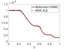
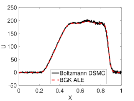
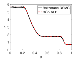
As already stated, we use this example also to consider the solutions of the BGK model for larger values of $\tau$ and compare them with those of the full Boltzmann equation. As before we use relaxation times $\tau$ according to equation (5). The density ratio between left and right part of the domain is again ${\rho_{l}}/{\rho_{r}}=8$, and we consider two more rarefied cases with $\rho_{l}=10^{-6},\rho_{l}=10^{-4}$, respectively, with corresponding values of the initial relaxation times $\tau_{l}=3.69\times 10^{-4},3.69\times 10^{-6}$ determined from (5). In the following figures 5 to 6 we have plotted the density, velocity and pressure obtained from the Boltzmann equation and the BGK model at the final time $0.0008$ . For the Boltzmann equation we consider a hard sphere monatomic gas. The solutions of the Boltzmann equation are obtained from a DSMC simulation averaging 20 independent runs. One observes in Fig. 5 and Fig. 6 that the solutions of the BGK model coincide with those of the Boltzmann equation for both values of the relaxation time $\tau$. Note that for the larger value of $\tau$, see Fig. 5, we have used a number of velocity grid points equal to $N_{v}=200$ to avoid oscillating solutions of the BGK model.

Fig. 5: Example 2: 1D shock tube. Comparison of the solutions obtained from the Boltzmann equation with DSMC and the BGK model with $N_{v}=200$ for $\rho_{l}=10^{-6}$ and the corresponding initial relaxation times $\tau_{l}=3.69\times 10^{-4}$.

Fig. 6: Example 2: 1D shock tube. Comparison of the solutions obtained from the Boltzmann equation with DSMC and the BGK model with $N_{v}=30$ for $\rho_{l}=10^{-4}$ and the corresponding initial relaxation times $3.69\times 10^{-6}$.

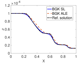
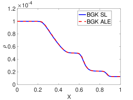
Furthermore, we compare the solutions of the BGK model obtained from the ALE method presented here with a higher order semi-Lagrangian (SL) scheme, see [7, 8]. We consider the initial densities $\rho_{l}=10^{-4}$. In Fig. 7 we have compared the densities obtained from ALE and SL scheme for different spatial resolutions. The solutions match perfectly well for a larger number of spatial grid points like $N_{x}=400$, see Fig. 7 on the right. We use this solution as the reference solution and compare it to the ALE and SL solutions for coarser grids. One observes that for $N_{x}=50$ and $N_{x}=100$ the solutions obtained from the ALE method deviates slightly from the reference solution, whereas the higher order SL solutions are still very near to the reference solution.

Fig. 7: Example 2: 1D shock tube. Comparison of the solutions obtained from the semi-Lagrange scheme and the ALE method with $N_{x}=50$ (left), $N_{x}=100$ (middle) and $N_{x}=400$ (right) for the BGK model with $N_{v}=30$ for $\rho_{l}=10^{-4}$ and the corresponding initial relaxation times $\tau_{l}=3.69\times 10^{-6}$.

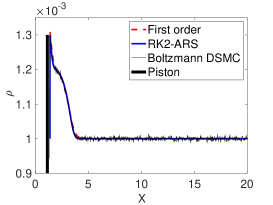
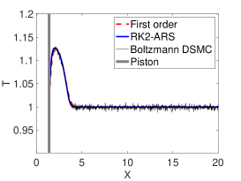
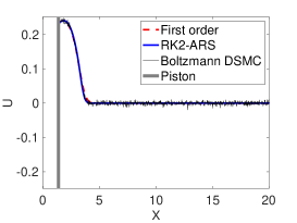
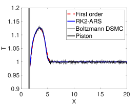
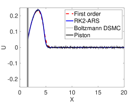
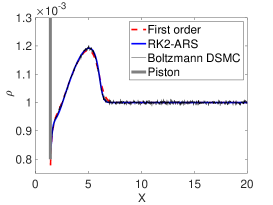
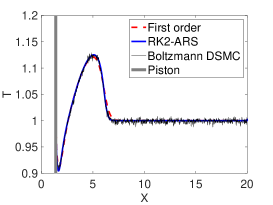
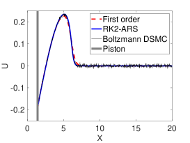
4.3 Example 3: Moving piston with prescribed velocity

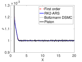
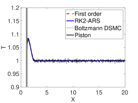
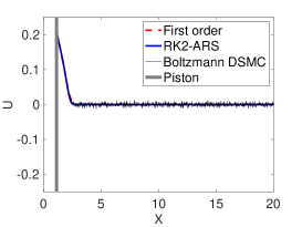
This problem has been considered in [12, 23] in a larger domain. We consider the one-dimensional domain $\Omega=[0,20]$. Initially the piston is positioned at $x=2$. We consider a total number $N_{x}=300$ grid points in physical space and $N_{v}=20$ grid points in velocity space. The left boundary moves with velocity

$$u_{p}=0.25*\sin(t).$$

Again we use non-dimensional variables with $R=1$. The initial velocity is $U_{0}=0$, the density $\rho_{0}=0.001$ and the temperature $T_{0}=1$. The minimum and maximum of the velocity are $v_{\rm min}=-10$ and $v_{\rm max}=10$. The initial distribution is the Maxwellian with the above initial macroscopic quantities. Initially particles are generated in the interval $[2,20]$. We have considered a fixed value of $\tau=1.83\cdot 10^{-2}$, a final time $t_{final}=4$ and a time step $\Delta t=0.001$. As in the previous section we compare the solutions obtained by the numerical method for the BGK equations to the solution obtained from a DSMC simulations of the full Boltzmann equation with a moving geometry, see [28]. For the DSMC method we use $\Delta x=20/900=2.22\cdot 10^{-2}$. In order to obtain a smooth solution for the DSMC simulations we have performed 50 independent runs.

Figure 8 to Figure 12 show the results for different times. When the piston starts to move in time, two situations occur: when the velocity is positive, the grid points are approaching each other. In this case one has to remove the grids points which are too close. We replace two grid points by a new one and locate it in the center between the two. When the velocity is negative new grid points have to be added. In both cases the distribution functions have to be updated in the additional grid points. This is done with the help of a least squares interpolation.

Fig. 8: Example 3: Moving piston. Comparison of ALE and DSMC methods at time $t=1$.

Fig. 9: Example 3: Moving piston. Comparison of ALE and DSMC methods at time $t=2$.

Fig. 10: Example 3: Moving piston. Comparison of ALE and DSMC methods at time $t=3$.

Fig. 11: Example 3: Moving piston. Comparison of ALE and DSMC methods at time $t=4$.

Fig. 12: Example 3: Moving piston. Zoom of the data obtained from ALE and DSMC methods at time $t=4$.

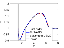
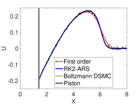
4.4 Example 4: Movement of a plate with pressure differences

We consider a computational domain as described in Figure 13 with $L=1$ and $l=0.1$.

Fig. 13: Example 4: Movement of a plate. Schematic view of a piston separating two subdomains with different temperature.

Initially, the center of mass of the plate is located at $X_{c}=0$. The gas and the plate are at rest. This problem has been studied in [12, 34]. We reconsider it as benchmark problem since an analytical expression is available for the equilibrium state. Using SI units, the initial temperature is $T_{0}=270$, gas constant $R=208$ and the initial pressures $P_{0}$ are the same on both sides of the plate and are equal to $0.0386$. The initial density $\rho_{0}$ is obtained from the equation of state. The initial Knudsen number is $0.08$ based on the characteristic length $2L$ and the relaxation time is fixed as $\tau=5.398\cdot 10^{-4}$. There are four boundary points, two are at the boundary of the domain and two are at the left and right end of the plate. The interior grid points are initialized with the spacing $\Delta x=2.2/200$ on the left and right of the plate. No grid points are initialized on the plate. The neighbor radius is given by $\Delta x=0.35h$ and the constant time step $\Delta t=2\cdot 10^{-6}$ is considered. We prescribe a higher temperature $T_{w}=330$ on the right side of plate and on the right boundary of the computational domain. On the left boundary of the plate and on the left boundary of the computational domain the temperature is fixed to $T_{0}$. Due to the high temperature on the right wall, the pressure on the right hand side starts to increase and the plate starts to move to the left hand side. The density of the plate is $10$ times larger than the density of the gas. This means, the mass of the plate is equal to $M=3.4366\cdot 10^{-5}$. The motion of the plate is computed from the Newton-Euler equations, where only a translational force is computed for the one dimensional case. Since the plate has two opposite normals $\pm 1$, from equations (9) and (10) the total force is given as the difference of pressure

$${F}=(\varphi_{\rm left}-\varphi_{\rm right})A,$$ (64)

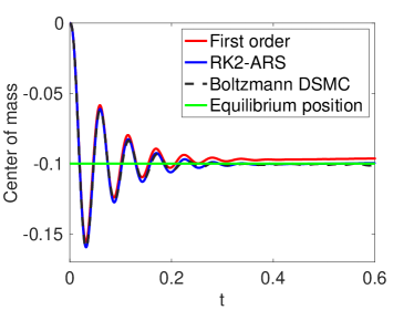
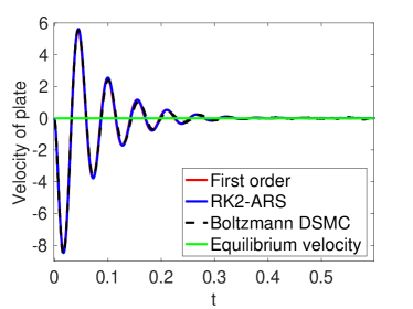
where $A$ is the area of the plate and $\varphi=\int_{\mathbb{R}}(v-U)^{2}g_{1}dv$. The plate starts oscillating and finally reaches the equilibrium position [12]

$$x_{\rm equi}=L\frac{(T_{0}-T_{w})}{(T_{0}+T_{w})}=-0.1.$$ (65)

We have compared the dynamics of the plate obtained from the ALE method with first and second order ARS schemes with a Boltzmann solution using the DSMC method. We observe that the oscillation of the plate obtained from both methods match. The simulations are performed up to the final time $t=0.6$ and the piston already reached the equilibrium at this time, see Figure 14. At the final time the simulated equilibrium position obtained from the first order method is $-9.639\cdot 10^{-3}$ and one given by the second order method is $-9.963\cdot 10^{-3}$ compared to the analytical solution which gives a value of $-0.1$, see (65). This yields an error of $3.7\%$ and $0.37\%$, respectively.

Fig. 14: Example 4: Movement of a plate. Comparison of position and velocity vs time of piston obtained from ALE and DSMC method

4.5 Example 5: The 2D-BGK model with smooth solution

For the convergence study we consider the BGK model with two-dimensional space and velocity domain for short time for a situation extending the one in section 4.1 to 2-D. The computational domain is $\Omega=[-1,1]\times[-1,1]$. The initial distribution is again the Maxwellian distribution and is given by

$$f(0,x,v)=\frac{\rho_{0}}{(2\pi RT_{0})^{3/2}}\exp{\left(-\frac{({v}-{U_{0}})^{2}}{2RT_{0}}\right)}$$

with $\rho_{0}=1,T_{0}=1,R=1$ and $U_{0}=(U_{0}^{(x)},U_{0}^{(y)},0)$ with

$$U_{0}^{(x)} = \frac{1}{\sigma}\left(\exp(\left(-(\sigma\sqrt{(x-0.2)^{2}+y^{2}}-1)^{2}\right)-2\exp\left(-(\sigma\sqrt{(x+0.2)^{2}+y^{2}}-1)^{2}\right)\right)$$

$$U_{0}^{(y)} = \frac{1}{\sigma}\left(\exp(\left(-(\sigma\sqrt{x^{2}+(y-0.2)^{2}}-1)^{2}\right)-2\exp\left(-(\sigma\sqrt{x^{2}+(y+0.2)^{2}}-1)^{2}\right)\right),$$

where $\sigma=10$. We have chosen again $\tau=10^{-5}$. Far field boundary conditions are applied on the boundaries with initial density, temperature and zero mean velocities. In order to perform the convergence study the time integration is carried out up to time $t=0.0208$, where the solution is still smooth. Different numbers of grid points are considered depending on the size of $h$. The initial grid spacing is $\Delta x=0.4~{}h$. The reference solution is the solution obtained from a grid with $h=0.013$, which corresponds to an initial number of grid points equal to $148996$. For the reference solution we use a time step equal to $\Delta t=2.6\cdot 10^{-5}$, which corresponds to a CFL condition with constant $0.5$. We refer to subsection 4.1 for a discussion of the CFL condition used here. This CFL number is also used for all other grid-sizes.

The convergence rate is determined by interpolating the temperature on $100$ grid points along $y=0$ for all grid sizes. In Figure 15 we have plotted the temperature obtained from the first order scheme and the ARS(2,2,1) scheme. Again, the ARS(2,2,2) scheme gives equivalent results. We note that we gain some computation time by using the ARS(2,2,1) scheme due to the additional function evaluations in the ARS(2,2,2) scheme.

Fig. 15: Example 5: 2D smooth solution. Temperature at $t=0.0208$ along $y=0$ for different $h$ obtained from the first order (left) and second order (right) schemes.

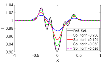
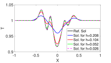
In Tables 7 and 8 we have presented the corresponding errors and the rate of convergence. It can be observed that the rates of convergence are as expected for the corresponding schemes.

$\Delta t$	$h$	$N_{x}$	$L^{1}$-error	Order	$L^{2}$ error	Order
$4.16\cdot 10^{-4}$	$0.208$	676	$5.57\cdot 10^{-2}$	$--$	$2.10\cdot 10^{-2}$	$--$
$2.08\cdot 10^{-4}$	$0.104$	2500	$1.01\cdot 10^{-2}$	$0.64$	$1.30\cdot 10^{-2}$	$0.69$
$1.04\cdot 10^{-4}$	$0.052$	9604	$5.18\cdot 10^{-3}$	$0.97$	$6.62\cdot 10^{-3}$	$0.98$
$5.20\cdot 10^{-5}$	$0.026$	37636	$1.93\cdot 10^{-3}$	$1.43$	$2.47\cdot 10^{-3}$	$1.42$

Table 7: Example 5: 2D smooth solution. Convergence of temperature at time $t=0.0208$ from the first order scheme.

$\Delta t$	$h$	$N_{x}$	$L^{1}$-error	Order	$L^{2}$ error	Order
$4.16\cdot 10^{-4}$	$0.208$	676	$1.48\cdot 10^{-2}$	$--$	$1.89\cdot 10^{-2}$	$--$
$2.08\cdot 10^{-4}$	$0.104$	2500	$5.71\cdot 10^{-3}$	$1.38$	$7.56\cdot 10^{-3}$	$1.33$
$1.04\cdot 10^{-4}$	$0.052$	9604	$1.15\cdot 10^{-3}$	$2.31$	$1.60\cdot 10^{-3}$	$2.34$
$5.20\cdot 10^{-5}$	$0.026$	37636	$2.49\cdot 10^{-4}$	$2.21$	$3.33\cdot 10^{-4}$	$2.27$

Table 8: Example 5: 2D smooth solution. Convergence of temperature at time $t=0.0208$ from the ARS(2,2,1) scheme.

4.6 Example 6: Moving 2D shuttle with prescribed velocity

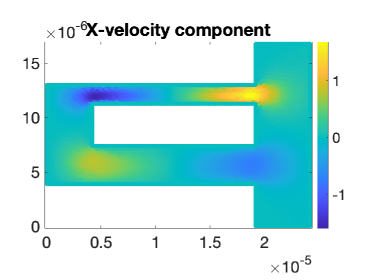
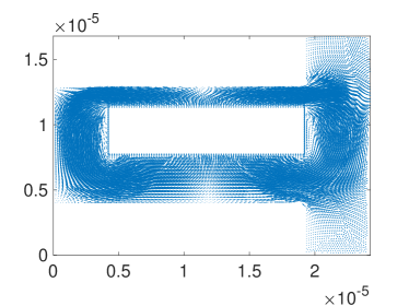
This example is an extension of Example 5 to two space dimensions. We use a 2D velocity space. We have taken this problem from the paper by Frangi et al. [16], where the authors have studied the biaxial accelerometer produced by STMicroelectronics with a surface micro-machining process. The authors have analysed the problem by considering a two-dimensional simplification. In Figure 16 we have sketched the computational domain in details. The shuttle lies initially in the middle of the domain. In the rest of the domain a gas flow is taking place. The shuttle oscillates with the velocity $v=v_{0}\cos(2\pi\nu t)$, where $\nu$ is the frequency. We use SI units in the following. We set $v_{0}=1$. The parameters mentioned in Figure 16 are $L_{1}=19.2\cdot 10^{-6},~{}d_{1}=4.2\cdot 10^{-6},~{}d_{2}=2.6\cdot 10^{-6},~{}d_{3}=5\cdot 10^{-6},~{}d_{4}=3.9\cdot 10^{-6},~{}d_{5}=18.8\cdot 10^{-6}$. We have changed the parameter $\nu$ in [16] and have chosen $\nu=40\cdot 4400$ Hz such that the maximum amplitude of the oscillations of the shuttle is half of the distance $d_{2}$ and the shuttle is not touching the boundaries of the domain. The initial pressure of the gas is equal to $0.125$ bar, which corresponds to an initial density $\rho_{0}=0.2$. These parameters give a relaxation time $\tau=1.73\times 10^{-9}$ which is fixed for all times.

The initial distribution $f_{0}$ of the gas is the Maxwellian with zero mean velocity, initial temperature $T_{0}=293$ and initial density $\rho_{0}$. A diffuse reflection boundary condition with wall temperature $T_{0}$ is applied on the solid lines and a far field boundary condition $f_{0}$ is applied on the dotted lines. We note that in the present investigation the time dependent motion of the shuttle is resolved, while in [16] the authors solve stationary equations with assigned non zero velocity on the boundary.

Fig. 16: Example 6: 2D shuttle. Geometry setup for moving $2D$ shuttle.

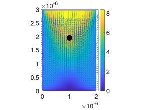
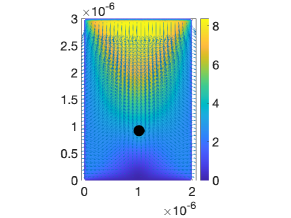
In Figure 17 we have plotted the velocity vector fields as well as $x$- and $y$- components of the velocity at times $t=1.2\cdot 10^{-6}$. Notice that the period of oscillations here is $T\approx 5.61\cdot 10^{-6}$. The total number of grid points is approximately $7000$ which gives $h=2.5\Delta x=4\cdot 10^{-7}$. The first order Euler scheme is used for the time integration with the time step $\Delta t=1.5\cdot 10^{-10}$.

Fig. 17: Example 6: 2D shuttle. First row: $x$- and $y$- velocity components at time $t=1.2\cdot 10^{-6}$. Second row: velocity fields at time $t=1.2\cdot 10^{-6}$.

4.6.1 Convergence study

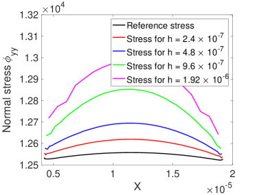
In Figure 18 we have plotted the normal stress tensor on the top wall of the shuttle at time $t=1.2\cdot 10^{-6}$. As a reference solution we consider the one obtained at the finest resolution with $h=1.2\cdot 10^{-7}$, which corresponds to approximately $111000$ grid points including boundary points. The finest time step is chosen as $8\cdot 10^{-11}$. The results of the convergence study are presented in Table 9.

Table 9 shows the results for the first order scheme in time and space. In order to estimate the error, we have generated a fixed number $N=100$ of points in equal distance at the upper boundary of the shuttle.

On these points we have interpolated the stress tensors from different resolutions including the reference solutions and then computed the errors. In Table 9 the $L^{1}$ and $L^{2}$ errors of the normal stress tensor $\varphi_{yy}$ are presented. The errors in the table show the first order convergence of the scheme.

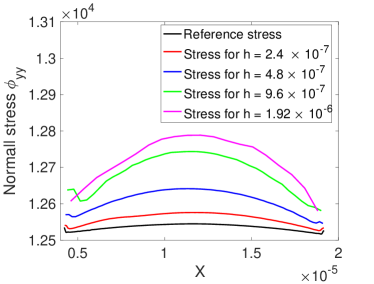
Table 10 shows the results for the ARS(2,2,1) scheme. We observe an improvement compared to the first order scheme, but we obtain in this situation a rate of convergence still below $2$, which is expected due to the non-smooth geometry.

Fig. 18: Example 6: 2D shuttle. The normal stress tensor on the top wall of the shuttle at $t=1.2\cdot 10^{-6}$ for different cell sizes. Left: First order in space and time. Right: Second order in space and time.

$\Delta t$	$h$	$L^{1}$-error	Order
$64\cdot 10^{-11}$	$1.92\cdot 10^{-6}$	$4.85\cdot 10^{-3}$	$--$
$32\cdot 10^{-11}$	$9.6\cdot 10^{-7}$	$3.27\cdot 10^{-3}$	$0.57$
$16\cdot 10^{-11}$	$4.8\cdot 10^{-7}$	$1.54\cdot 10^{-3}$	$1.08$
$8\cdot 10^{-11}$	$2.4\cdot 10^{-7}$	$7.04\cdot 10^{-4}$	$1.13$

Table 9: Example 6: 2D shuttle. Convergence of the normal stress tensor $\phi$ on the top wall of the shuttle at time $t=1.2\cdot 10{-6}$ from the first order scheme in space and time.

$\Delta t$	$h$	$L^{1}$-error	Order
$96\cdot 10^{-11}$	$1.92\cdot 10^{-6}$	$2.73\cdot 10^{-3}$	$--$
$48\cdot 10^{-11}$	$9.6\cdot 10^{-7}$	$2.22\cdot 10^{-3}$	$0.30$
$24\cdot 10^{-11}$	$4.8\cdot 10^{-7}$	$1.09\cdot 10^{-3}$	$1.03$
$12\cdot 10^{-11}$	$2.4\cdot 10^{-7}$	$3.55\cdot 10^{-4}$	$1.62$

Table 10: Example 6: 2D shuttle. Convergence of the normal stress tensor $\phi$ on the top wall of the shuttle at time $t=1.2\cdot 10^{-6}$ from the ARS(2,2,1) scheme.

4.7 Example 7: Transport of rigid particles

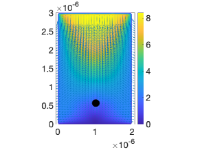
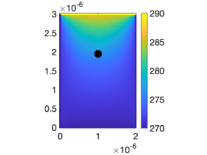
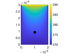
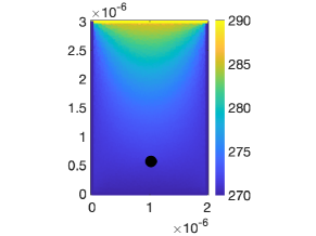
The main aim of the following tests is to demonstrate the ability of the scheme to simulate arbitrary shapes of rigid body motion immersed in a rarefied gas. We consider again two dimensional physical and velocity space. In the previous 2-D test case a one-way coupling of rigid body motion and gas was investigated. In the present example we consider a two-way coupling, where the gas is also influencing the motion of the rigid body. Using SI units, we consider the computational domain $\Omega=[0,2\cdot 10^{-6}]\times[0,3\cdot 10^{-6}]$. The initial density is $\rho_{0}=1$, the initial temperature $T_{0}=270$ and the initial mean velocity $U_{0}=(0,0)$. These parameters yield the initial relaxation time $\tau=3.71\times 10^{-10}$ which is fixed for all times. On the top we prescribe a Maxwellian with parameters $\rho=\rho_{0},T=290,U=U_{0}$. On the bottom boundary we use a diffuse reflection boundary condition with wall temperature $T_{w}=T_{0},U_{w}=U_{0}$.

On the left and right wall we apply far field boundary conditions, that means, we prescribe a Maxwellian with initial parameters $\rho_{0},T_{0},U_{0}$. On the rigid body we apply a diffuse reflection boundary condition with temperature $T(t,x)$ and velocity $U(t,x)$. We consider circular as well as chiral particles. For the following simulations we use the first order scheme in space and time.

4.7.1 Transportation of a circular particle

First we consider a circular particle of radius $0.1\cdot 10^{-6}$ and initial center of mass $(1.0\cdot 10^{-6},2.5\cdot 10^{-6})$. The grid points are generated equidistantly with $h=2.5\Delta x=5.25\cdot 10^{-8}$ which gives an initial number of grid points equal to $7273$. The time step is $\Delta t=1\cdot 10^{-11}$.

In Figures 19 and 20 we have plotted the positions of the circular particle together with velocity fields and temperature fields, respectively, at times $1\cdot 10^{-7},3\cdot 10^{-7}$ and $4.5\cdot 10^{-7}$.

Fig. 19: Example 7: Circular particles. Particle positions and velocity field at $t=1\cdot 10^{-7}$, $t=3\cdot 10^{-7}$ and $t=4.5\cdot 10^{-7}$.

Fig. 20: Example 7: Circular particles. Particle positions and temperature field at $t=1\cdot 10^{-7}$, $t=3\cdot 10^{-7}$ and $t=4.5\cdot 10^{-7}$.

4.7.2 Transportation of a chiral particle

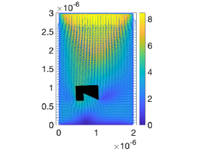
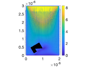
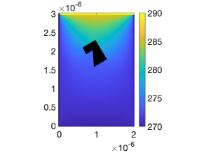
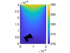
In this example, we consider a chiral particle with initial center of mass $(1.0\cdot 10^{-6},2.3\cdot 10^{-6})$. We have used a relatively fine grid with $h=6.25\cdot 10^{-8}$, which gives $9528$ particles and a time step $\Delta t=1\cdot 10^{-11}$. The boundary conditions are the same as in the case of the circular particle in the previous subsection.

In Figures 21 and 22 we have plotted the positions of the chiral particle together with velocity fields and temperature fields, respectively, at times $1\cdot 10^{-7},3\cdot 10^{-7}$ and $4.5\cdot 10^{-7}$.

Fig. 21: Example 7: Chiral particles. Particle positions and velocity field at $t=1\cdot 10^{-7}$, $t=3\cdot 10^{-7}$ and $t=4.5\cdot 10^{-7}$

Fig. 22: Example 7: Chiral particles. Particle positions and temperature field at $t=1\cdot 10^{-7}$, $t=3\cdot 10^{-7}$ and $t=4.5\cdot 10^{-7}$.

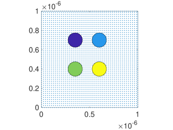
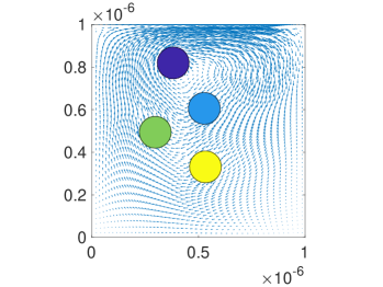
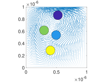
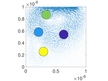
4.8 Multiple rigid particles in a driven cavity

We consider a square cavity $[0,L]\times[0,L]$ with $L=1\cdot 10^{-6}$. The initial parameters of the Maxwellian are the same as in the previous test case. Diffuse reflection boundary conditions with temperature $T_{0}$ are applied on all boundaries as well as on the rigid particles. At the top wall we prescribe a non-zero velocity in $x$-direction given by

$$U_{0}^{(x)}=10\left(\frac{2x}{L}\right)^{2}\left(2-\left(\frac{2x}{L}\right)^{2}\right).$$

This leads to a maximum velocity equal to $10$ at the center of the wall. The $y$-component of the top wall velocity is zero. The velocities on all other walls and on the rigid particles are zero. We have generated 4 rigid particles of radius $0.075L$ with initial position as in Figure 23, first panel. The numerical particles are generated according to the parameter $h=5.25\cdot 10^{-8}$ which gives, initially, a total number of $2313$ particles. The time step is chosen as $\Delta t=1\cdot 10^{-11}$.

Fig. 23: Example 8: Multiple particles in a driven cavity. Particle positions and velocity field. First row: $t=0$ and $t=1.5\cdot 10^{-7}$. Second row $t=3\cdot 10^{-7}$ and $t=6\cdot 10^{-7}$.

5 Conclusion and Outlook

In this paper, we have presented an Arbitrary Lagrangian-Eulerian method for the simulation of the BGK equation with moving boundaries. Besides the ALE approach, the method is based on first and second order least squares approximations. Several numerical tests are performed in order to validate the method, both in one and two space dimensions. Moreover, we compared the results with those obtained by DSMC solution of the Boltzmann equation and by a higher order conservative semi-Lagrangian scheme.

In particular, in 1D we consider the case of a moving plate immersed in a rarefied gas. In a first test we assume that the motion of the plate is prescribed (one way coupling), while in a second test the motion of the plate is computed from Newton’s equations (two way coupling). In two space dimensions we considered several test problems. A first test case investigates a situation where the motion of the object is prescribed (one -way coupling). We consider the motion of a shuttle in a 2D model of a Micro Electro Mechanical System, see [16]. Moreover, we considered some tests with rigid bodies/mesoscopic particles of arbitrary shape immersed in a gas and driven by either thermophoresis or driven cavity flow (two way coupling).

In future work the scheme will be extended to the case of gas-mixtures [18] and to three space dimensions. Moreover, larger collections of mesoscopic particles dispersed in a rarefied gas will be considered, thus providing a quantitative tool that can be used to validate homogenised macroscopic models of suspensions.

References

- [1] D. Avesani, M. Dumbser, A. Bellin, A new class of Moving-Least-Squares WENO-SPH schemes. J. Comput. Phys., 270:278-299, 2014.
- [2] D. Avesani, M. Dumbser, R. Vacondio, M. Righetti, An alternative SPH formulation: ADER-WENO-SPH. Computer Methods in Applied Mechanics and Engineering, 382:113871, 2021.
- [3] R. R. Arslanbekov, V. I. Kolobov, A. A. Frolova, Immersed boundary method for Boltzmann and Navier-Stokes solvers with adaptive cartesian mesh. AIP Conference Proceedings, 1333(1):873-877, 2011.
- [4] U. Ascher, S. Ruth, R.J. Spiteri, Implicit-explicit Runge-Kutta Methods for Time Dependent PDEs. Appl. Numer. Math., 25: 151-161, 1997.
- [5] T. Baier, S. Tiwari, S. Shrestha, A. Klar, H. Hardt, Thermophoresis of Janus particles at large Knudsen numbers. Phys. Rev. Fluids, 3:094202, 2018.
- [6] C. K. Chu, Kinetic-theoretic description of the formation of a shock wave, Phys. Fluids 8:12–22, 1965.
- [7] S. Y. Cho, S. Boscarino, G. Russo, S.-B. Yun, Conservative semi-Lagrangian schemes for kinetic equations - Part I: Reconstruction. J. Comput. Phys., 432:110951, 2021.
- [8] S. Y. Cho, S. Boscarino, G. Russo, S.-B. Yun, Conservative semi-Lagrangian schemes for kinetic equations Part II: Applications. J. Comp. Phys., 436:110281, 2021.
- [9] . S. Chapman, T. W. Cowling, The Mathematical Theory of Non-Uniform Gases, Cambridge University Press, 1970.
- [10] A. Chertock, A. Coco, A. Kurganov, G. Russo, A second-order finite-difference method for compressible fluids in domains with moving boundaries. Communications in Computational Physics, 23:230-263, 2018.
- [11] P. Degond, G. Dimarco, L. Pareschi, The moment-guided Monte Carlo method. Int. J. Num. Meth. Fluids, 67:189-213. 2011.
- [12] G. Dechristé, L. Mieussens Numerical simulation of micro flows with moving obstacles. Journal of Physics: Conference Series 362: 012030, 2012.
- [13] G. Dechristé, L. A. Mieussens, Cartesian cut cell method for rarefied flow simulations around moving obstacles. J. Comput. Phys. 314, 454–488, 2-16.
- [14] G. Dimarco, L. Pareschi, Numerical methods for kinetic equations. Acta Numerica, 23:369-520, 2014.
- [15] C. Drumm, S. Tiwari, J. Kuhnert, H.-J. Bart, Finite pointset method for simulation of the liquid–liquid flow field in an extractor. Computers & Chemical Engineering, 32(12):2946-2957, 2008.
- [16] A. Frangi, A. Frezzotti, S. Lorenzani, On the application of the BGK kinetic model to the analysis of gas-structure interactions in MEMS. Computers and Structures, 85:810-817, 2007.
- [17] M. Groppi, G. Russo, G. Stracquadanio, High order semi-Lagrangian methods for the BGK equation . Commun. Math. Sci., 14(2):389-417, 2007.
- [18] M. Groppi, G. Russo, G. Stracquadanio, Semi-Lagrangian Approximation of BGK Models for Inert and Reactive Gas Mixtures . P., Soares A. (eds) From Particle Systems to Partial Differential Equations. PSPDE 2016. Springer Proceedings in Mathematics & Statistics , 258, 2018.
- [19] G. Karniadakis, A. Beskok, N. Aluru, Microflows and Nano- flows: Fundamentals and Simulations. Springer, New York, 2005.
- [20] J. Kuhnert, General smoothed particle hydrodynamics. PhD Thesis, University of Kaiserslautern, Germany, 2999.
- [21] T. Liska, J. Orkisz, The finite difference method on arbitrary irregular grid and its application in applied mechanics. Computers and Structures, 11:83-95, 1980.
- [22] S. Pieraccini, G. Puppo, Implicit-Explicit Schemes for BGK Kinetic Equations. J. Sci. Comput., 32:1-28, 2007.
- [23] G. Russo, F. Filbet, Semi-Lagrangian schemes applied to moving boundary problems for the BGK model of rarefied gas dynamics. Kinetic and Related Model, Amer. Inst. Math. Sci. 2:231–250, 2009.
- [24] G. A. Sod, A survey of several finite difference methods for systems of nonlinear hyperbolic conservation laws. J. Comp. Phys., 27:1-31, 1978.
- [25] T. Sonar, Difference operators from interpolating moving least squares and their deviation from optimality . ESAIM:M2AN, 39(5):883-908, 2005.
- [26] P. Suchde, J. Kuhnert, S. Tiwari, On meshfree GFDM solvers for the incompressible Navier-Stokes equations. Computers and Fluids, 165:1-12, 2018.
- [27] S. Shrestha, S. Tiwari, A. Klar, Comparison of numerical simulations of the Boltzmann and the Navier-Stokes equations for a moving rigid circular body in a micro scaled cavity. Int. J. Adv. Eng. Sci. App. Math. , 7(1-2):38-50, 2015.
- [28] S. Shrestha, S. Tiwari, A. Klar, S. Hardt, Numerical Simulation of a moving rigid body in a rarefied gas. J. Comput. Phys., 292:239-252, 2015.
- [29] T. Tsuji, K. Aoki, Moving boundary problems for a rarefied gas: Spatially one dimensional case. J Comput Phys 250:574–600, 2013.
- [30] T. Tsuji, K. Aoki, Gas motion in a microgap between a stationary plate and a plate oscillating in its normal direction. Microfluid Nanofluid, 16:1033-1045, 2014.
- [31] S. Tiwari, J. Kuhnert, Modelling of two-phase flow with surface tension by Finite Point-set method (FPM). J. Comp. Appl. Math., 203:376-386, 2007.
- [32] S. Tiwari, A. Klar, S. Hardt, A particle-particle hybrid method for kinetic and continuum equations, J . Comp. Phys. 228:7109-7124, 2009.
- [33] S. Tiwari, A. Klar, S. Hardt, A. Donkov, Coupled solution of the Boltzmann and Navier–Stokes equations in gas–liquid two phase flow, Computers and Fluids 71:283-296, 2013.
- [34] S. Tiwari, A. Klar, G. Russo, A meshfree method for solving BGK model of rarefied gas dynamics . Int. J. Adv. Eng. Sci. Appl. Math., 11(3):187-197, 2019.
- [35] S. Tiwari, A. Klar, G. Russo, Interaction of rigid body motion and rarefied gas dynamics based on the BGK model, Mathematics in Engineering, 2(2): 203-229, 2020.
- [36] G. Voronoi, Nouvelles applications des parameters continus la theorie des formes quadratiques. J. Reine Angew. Math., 133:161, 1907.
- [37] T. Xiong, G. Russo, J.-M. Qiu, Conservative Multi-Dimensional Semi-Lagrangian Finite Difference Scheme: Stability and Applications to the Kinetic and Fluid Simulations. arXiv:1607.07409v1, 2016.
- [38] C. Zhang, G.M. Xiang, B. Wang, X.Y. Hu, N.A. Adams, A weakly compressible SPH method with WENO reconstruction. J. Comput. Phys., 392(1), 1-18, 2019.