Incompatibility measures in multi-parameter quantum estimation under hierarchical quantum measurements

Abstract

The incompatibility of the measurements constraints the achievable precisions in multi-parameter quantum estimation. Understanding the tradeoff induced by such incompatibility is a central topic in quantum metrology. Here we provide an approach to study the incompatibility under general $p$-local measurements, which are the measurements that can be performed collectively on at most $p$ copies of quantum states. We demonstrate the power of the approach by presenting a hierarchy of analytical bounds on the tradeoff among the precision limits of different parameters. These bounds lead to a necessary condition for the saturation of the quantum Cramér-Rao bound under $p$-local measurements, which recovers the partial commutative condition at p=1 and the weak commutative condition at $p=\infty$. As a further demonstration of the power of the framework, we present another set of tradeoff relations with the right logarithmic operators(RLD).

I Introduction

By utilizing quantum mechanical effects, such as superposition and entanglement, quantum metrology can achieve better precision limit than classical metrology. There is now a good understanding on the local precision limit for single-parameter quantum estimation, where the precision limit can be quantified by the single-parameter quantum Cramér-Rao boundHels76book ; Hole82book ; BrauCM96 ; GiovLM04 ; GiovLM06 ; Escher2011 ; Naga07beating ; HiggBBW07 ; XianHBW11 ; Slus17unconditional ; daryanoosh2018experimental ; yuan2017quantum ; yuan2017M ; Liu2022 . Practical applications, however, typically involve multiple parameters, for which the precision limits are much less understoodMatsumoto_2002 ; PhysRevLett.111.070403 ; PhysRevLett.119.130504 ; Haya05book ; Hou20minimal ; Federico2021 ; Houeabd2986 ; HouSuper2021 ; Yang2019 ; PhysRevLett.116.180402 ; Zhu2018universally ; Magdalena2016 ; PhysRevLett.123.200503 ; GillM00 ; ALBARELLI2020126311 ; Carollo_2019 ; Lu2021 ; Ragy2016 ; Chen_2017 ; Liu_2019 ; ChenHZ2019 ; Francesco2019 ; Rafal2020 ; Kok2020 ; vidrighin2014 ; crowley2014 ; Yue2014 ; Zhang2014 ; Liu2017 . Due to the incompatibility of the optimal measurements for different parameters, the multi-parameter quantum Cramér-Rao bound is in general not achievable. Tradeoffs among the precisions of different parameters have to be made. Quantifying such tradeoff is now one of the main subjects in quantum metrologyGillM00 ; ALBARELLI2020126311 ; Carollo_2019 ; Lu2021 ; Ragy2016 ; Chen_2017 ; Liu_2019 ; ChenHZ2019 ; Francesco2019 ; Rafal2020 ; Kok2020 ; vidrighin2014 ; crowley2014 ; Yue2014 ; Zhang2014 ; Liu2017 ; Roccia_2017 ; e22111197 ; Candeloro2021 ; Koichi2013 ; Kahn2009 ; Yuxiang2019 ; Suzuki2016 ; Sidhu2021 .

The incompatibility of the measurements is rooted in the prohibition of simultaneous measurement of non-commutative observables, which is one of the defining features of quantum mechanics. Previous studies on the incompatibility mostly focus on the extreme cases: either the measurement is separable or can be performed collectively on infinite copies of quantum states. When the measurements can be performed on infinite number of identical copies of quantum states, the Holevo bound quantifies the achievable precision Hole82book ; Koichi2013 ; Kahn2009 ; Yuxiang2019 . Except for few special casesSuzuki2016 ; Sidhu2021 , the Holevo bound in general can only be evaluated numericallyPhysRevLett.123.200503 . In practise the measurements typically can only be performed collectively on a finite number of quantum states, under which the Holevo bound is also not achievable in general. In the case of two parameters, Nagaoka provided a bound under the separable measurements which is tighter than the Holevo boundNagaoka1 ; Nagaoka2 . Conlon et al. recently generalized the Nagaoka bound to more than two parameters, which in general requires numerical optimizationConlon2021 . Gill-Massar bound provided an analytical measure on the tradeoff induced by the incompatibility of the separable measurementsGillM00 . For collective measurements on at most $2$ copies of quantum states, Zhu and Hayashi have obtained a tradeoff relation for completely unknown statesZhu2018universally . However, the incompatibilities under general $p$-local measurements, which are the measurements that can be performed collectively on at most $p$ copies of quantum states, are little understood.

Here we provides a framework to study the precision under general $p$-local measurements. This approach leads to new multi-parameter precision bounds which include the Holevo bound and the Nagaoka bound as special cases. We also provide a systematic way to generate hierarchical analytical tradeoff relations under general $p$-local measurements. The obtained tradeoff relations provide a necessary condition for the saturation of the multi-parameter quantum Cramér-Rao bound under $p$-local measurements, which recovers the partial commutative conditionYang2019 at $p=1$ and the weak commutative condition at $p=\infty$. Our study thus not only provides a framework that can generate new analytical bounds on the tradeoff under general $p$-local measurements, but also provides a coherent picture for the existing results on the extreme cases.

The article is organized as following: in Sec.II we introduce the notations and list the main results; in Sec.III we present analytical tradeoff relations for pure states; in Sec.IV we provide new multi-parameter precision bounds for mixed states and use it to derive analytical tradeoff relations for mixed states. The tradeoff relations leads to a necessary condition for the saturation of the QCRB and we show how it reduces to the partial commutative condition at $p=1$ and the weak commutative condition at $p\rightarrow\infty$; in Sec. V we demonstrate the versatility of the approach by presenting another set of tradeoff relations in terms of the right logarithmic derivative; in Sec.VI some examples are presented and Sec.VII concludes.

II Precision limit in quantum metrology

We first introduce the notations and terminologies that are used in this article and list the main results.

For the single-parameter quantum estimation, given a parametrized state, $\rho_{x}$, with $x$ as the parameter to be estimated, by performing a positive operator valued measurement(POVM), denoted as $\{M_{\alpha}\}$, on the state, we can get the measurement result, $\alpha$, with a probability $p(\alpha|x)=Tr(\rho_{x}M_{\alpha})$. The variance of any locally unbiased estimator, $\hat{x}$, is then lower bounded by the Cramér-Rao boundCram46 ; Fish22 as $\delta\hat{x}^{2}\geq\frac{1}{\nu F_{C}}$, here $\delta\hat{x}^{2}=E[\hat{x}-x]^{2}$ is the variance of the unbiased estimator, $F_{C}=\int_{\alpha}\frac{1}{p(\alpha|x)}(\frac{\partial_{x}p(\alpha|x)}{\partial x})^{2}d\alpha$ is the Fisher informationFish22 , $\nu$ is the number of repetitions of the procedure, which is assumed to be asymptotically large. By optimizing the POVM, we get the quantum Cramér-Rao bound(QCRB) Hels76book ; Hole82book ,

$$\delta\hat{x}^{2}\geq\frac{1}{\nu F_{C}}\geq\frac{1}{\nu F_{Q}},$$ (1)

here $F_{Q}$ is the quantum Fisher information (QFI), which is the maximization of the Fisher information over all POVMHels76book ; Hole82book . The QFI can be computed directly from the quantum state as $F_{Q}=Tr(\rho_{x}L^{2})$, here $L$ is the symmetric logarithmic operator(SLD) which is implicitly defined via the equation $\frac{\partial\rho_{x}}{\partial x}=\frac{1}{2}(L\rho_{x}+\rho_{x}L)$. For single-parameter estimation, the QCRB can always be saturated with the POVM performed separately on each copy of the state. One POVM that saturates the single-parameter QCRB is the projective measurement on the eigenvectors of the SLD.

For multi-parameter quantum estimation, where $x=(x_{1},\cdots,x_{n})$ with $n\geq 2$, the quantum Fisher information becomes the quantum Fisher information matrix with the $jk$-th entry given by

$$(F_{Q})_{jk}=Tr(\rho_{x}\frac{L_{j}L_{k}+L_{k}L_{j}}{2}),$$ (2)

here $L_{q}$ is the SLD corresponds to the parameter $x_{q}$, which satisfies $\partial_{x_{q}}\rho_{x}=\frac{1}{2}(\rho_{x}L_{q}+L_{q}\rho_{x})$, $\forall q\in\{1,\cdots,n\}$. The multi-parameter quantum Cramér-Rao bound is given by

$$Cov(\hat{x})\geq\frac{1}{\nu}F_{Q}^{-1},$$ (3)

where $Cov(\hat{x})$ is the covariance matrix for locally unbiased estimators, $\hat{x}=(\hat{x}_{1},\cdots,\hat{x}_{n})$, with the $jk$-th entry given by $Cov(\hat{x})_{jk}=E[(\hat{x}_{j}-x_{j})(\hat{x}_{k}-x_{k})]$, $\nu$ is the number of copies of quantum states. In this article, we assume $F_{Q}$ is non-singular so $F_{Q}^{-1}$ exists, in which case $Cov(\hat{x})\geq\frac{1}{\nu}F_{Q}^{-1}>0$ is also non-singular.

Different from the single-parameter quantum estimation, the multi-parameter quantum Cramér-Rao bound is in general not saturable. This is due to the incompatibility of the optimal measurements for different parameters. Such incompatibility is rooted in the prohibition of simultaneous measurement of non-commutative observables and its manifested effect in multi-parameter estimation is the tradeoff on the precision limits for the estimation of different parameters.

We can quantify the incompatibility through either $\frac{1}{\nu}Tr[F_{Q}^{-1}Cov^{-1}(\hat{x})]$ALBARELLI2020126311 or $\nu Tr[F_{Q}Cov(\hat{x})]$ ALBARELLI2020126311 ; Federico2021 ; Carollo_2019 , which measures how close $Cov(\hat{x})$ is to $\frac{1}{\nu}F_{Q}^{-1}$. These two quantities are roughly reciprocal to each another. Compared to the other quantities, such as $\|\nu Cov(\hat{x})-F_{Q}^{-1}\|$ or $\|\frac{1}{\nu}Cov^{-1}(\hat{x})-F_{Q}\|$, $\frac{1}{\nu}Tr[F_{Q}^{-1}Cov^{-1}(\hat{x})]$ and $\nu Tr[F_{Q}Cov(\hat{x})]$ both have the advantage of being invariant under reparametrization. In this article we will use $\Gamma=\frac{1}{\nu}Tr[F_{Q}^{-1}Cov^{-1}(\hat{x})]$ as the measure. When the QCRB is saturable, $Cov(\hat{x})=\frac{1}{\nu}F_{Q}^{-1}$, $\Gamma=Tr(I_{n})=n$, here $I_{n}$ denotes the $n\times n$ Identity matrix. This is the maximal value $\Gamma$ can achieve. When the QCRB is not saturable we have $\Gamma<n$. The gap between $n$ and $\Gamma$ quantifies the incompatibility. We will denote the measure under the $p$-local measurement as $\Gamma_{p}=\frac{1}{\nu}Tr[F_{Q}^{-1}Cov^{-1}(\hat{x})]$ with $Cov(\hat{x})$ as the covariance matrix achieved under the optimal $p$-local measurement. The gap between $n$ and $\Gamma_{p}$ decreases with $p$ since the measurements become less restrictive when $p$ increases, we thus have $\Gamma_{1}\leq\Gamma_{2}\leq\cdots\leq\Gamma_{\infty}$. For pure states, however, we have $\Gamma_{1}=\Gamma_{2}=\cdots=\Gamma_{\infty}$ since for pure states the optimal measurement can be taken as the 1-local measurement Matsumoto_2002 .

The existing results on the incompatibility are mostly on the extreme cases with either $p=\infty$ or $p=1,2$.

For $p=\infty$, the precision limit can be characterized by the Holevo boundHole82book , which is given by $\nu Tr[WCov(\hat{x})]\geq\min_{\{X_{j}\}}\{Tr[WReZ(X)]+\|\sqrt{W}ImZ(X)\sqrt{W}\|_{1}\}$, where $W\geq 0$ is a weighted matrix, $Z(X)$ is a matrix with its $jk$-th entry given by $Z(X)_{jk}=Tr(\rho_{x}X_{j}X_{k})$, here $\{X_{1},\cdots,X_{n}\}$ is a set of Hermitian operators that satisfy the local unbiased condition, $Tr(\rho_{x}X_{j})=0$ for any $j\in\{1,\cdots,n\}$ and $Tr(\partial_{x_{k}}\rho_{x}X_{j})=\delta_{k}^{j}$ with $\delta_{k}^{j}$ as the Kronecker delta, $\delta_{k}^{j}=1$ when $k=j$ and $\delta_{k}^{j}=0$ when $k\neq j$, $ReZ(x)=\frac{Z(x)+Z^{T}(x)}{2}$ is the real part of $Z(x)$, $ImZ(x)=\frac{Z(x)-Z^{T}(x)}{2i}$ is the imaginary part. The Holevo bound can only be evaluated numerically in generalPhysRevLett.123.200503 . For pure states, the Holevo bound can be saturated by $1$-local measurementsMatsumoto_2002 . For mixed states, the saturation of the Holevo bound in general requires collective measurements on infinite copies of the state.

A necessary and sufficient condition for the Holevo bound to coincide with the QCRB is $Tr(\rho_{x}[L_{j},L_{k}])=0$ for any $j,k\in\{1,\cdots,n\}$. This is called the weak commutative condition. When the weak commutative condition holds, there exists collective measurements on infinite copies of quantum states under which the QCRB is saturated and $\Gamma_{\infty}=n$.

As the Holevo bound corresponds to the minimal value upon all choice of $\{X_{j}\}$, by making a particular choice of $\{X_{j}\}$ as $X_{j}=\sum_{k}(F_{Q}^{-1})_{jk}L_{k}$ and $W=F_{Q}$, we haveCarollo_2019

$$\nu Tr[F_{Q}Cov(\hat{x})]\leq n+\|F_{Q}^{-\frac{1}{2}}F_{Im}F_{Q}^{-\frac{1}{2}}\|_{1}\leq 2n,$$ (4)

here $F_{Im}$ is a matrix with the $jk$-th entry given by $(F_{Im})_{jk}=\frac{1}{2i}Tr(\rho_{x}[L_{j},L_{k}])$. The last inequality is obtained from the fact that $F_{Q}+iF_{Im}\geq 0$, which leads to $\|F_{Q}^{-\frac{1}{2}}F_{Im}F_{Q}^{-\frac{1}{2}}\|_{1}\leq Tr(F_{Q}^{-\frac{1}{2}}F_{Q}F_{Q}^{-\frac{1}{2}})=n$. Through the Cauchy-Schwarz inequality,

$$\begin{aligned} &Tr[F_{Q}Cov(\hat{x}]Tr[F_{Q}^{-1}Cov^{-1}(\hat{x})]\\ &\geq|Tr[F_{Q}^{\frac{1}{2}}Cov^{\frac{1}{2}}(\hat{x})Cov^{-\frac{1}{2}}(\hat{x})F_{Q}^{-\frac{1}{2}}]|^{2}=n^{2},\end{aligned}$$ (5)

this leads to a lower bound on $\Gamma_{\infty}$ asFederico2021

$$\Gamma_{\infty}=\frac{1}{\nu}Tr[F_{Q}^{-1}Cov^{-1}(\hat{x})]\geq\frac{n^{2}}{n+\|F_{Q}^{-\frac{1}{2}}F_{Im}F_{Q}^{-\frac{1}{2}}\|_{1}}.$$ (6)

We note that the lower bound on $\Gamma_{\infty}$ is not sufficient to decide the incompatibility of the measurements at $p=\infty$ as it can not tell whether $\Gamma_{\infty}$ can reach $n$ and furthermore how close $\Gamma_{\infty}$ is to $n$. The upper bound is more informative in this sense. As if there exists an upper bound which is less than $n$, we can tell for sure that the measurements are incompatible, and furthermore the gap between $n$ and the upper bound provides a measure on the incompatibility. To our knowledge, except the trivial bound, $\Gamma_{\infty}\leq n$, there were no analytical upper bounds on $\Gamma_{\infty}$ even at the extreme case with $p=\infty$.

For the other extreme case with $p=1$, Nagaoka provided a bound on the precision limit in the case of two parameters($n=2$)Nagaoka1 ; Nagaoka2 , which is given by

$$\nu Tr[Cov(\hat{x})]$$ (7)

$$\geq \min_{\{X_{1},X_{2}\}}Tr(\rho_{x}X_{1}^{2})+Tr(\rho_{x}X_{2}^{2})+\|\sqrt{\rho_{x}}[X_{1},X_{2}]\sqrt{\rho_{x}}\|_{1},$$

where $\{X_{1},X_{2}\}$ are two Hermitian operators satisfying the locally unbiased condition. The Nagaoka bound in general can only be evaluated numerically and is tighter than the Holevo bound. Recently the Nagaoka bound has been generalized to $n$ parameters which also requires numerical evaluation Conlon2021 .

Gill and Massar provided an analytical upper bound on $\Gamma_{1}$ asGillM00

$$\Gamma_{1}\leq d-1,$$ (8)

here $d$ is the dimension of the Hilbert space for a single $\rho_{x}$. The Gill-Massar bound is nontrivial only when $n>d-1$. Recent studies have also obtained some tradeoff relations with the Ozawa’s uncertainty relation for pairs of parametersLu2021 .

A necessary condition for the saturation of the QCRB under 1-local measurements is the partial commutative conditionYang2019 , which requires all SLDs commute on the support of $\rho_{x}$. Specifically if we write $\rho_{x}$ in the eigenvalue decomposition as $\rho_{x}=\sum_{1}^{m}\lambda_{i}|\Psi_{i}\rangle\langle\Psi_{i}|$ with $\lambda_{i}>0$, the partial commutative condition is $\langle\Psi_{r}|[L_{j},L_{k}]|\Psi_{s}\rangle=0$ for any $j,k\in\{1,\cdots,n\}$, and any $r,s\in\{1,\cdots,m\}$. The connection between the partial commutative condition and the weak commutative condition remained openYang2019 .

For $p=2$, Zhu and Hayashi provided an upper bound on $\Gamma_{2}$ as

$$\Gamma_{2}=\frac{1}{\nu}Tr[F_{Q}^{-1}Cov^{-1}(\hat{x})]\leq\frac{3}{2}(d-1),$$ (9)

which is nontrivial only when $n>\frac{3}{2}(d-1)$.

For general $p$, the incompatibility is little understood. In this article, we provide a framework to study the incompatibility under general $p$-local measurements. This framework provides new precision bounds that include the Holevo bound and the Nagaoka bound as special cases, and leads to nontrivial analytical upper bounds for general $\Gamma_{p}$. A necessary condition for the saturation of the QCRB can also be obtained, which recovers the partial commutative condition at $p=1$ and the weak commutative condition at $p\rightarrow\infty$. The new multi-parameter precision bounds are presented in Sec.IV.1, here we first list the analytical upper bounds and the necessary condition for the saturation of QCRB under general p-local measurements.

1. For pure states, we have

   $$\begin{aligned} \frac{1}{\nu}Tr[F_{Q}^{-1}Cov^{-1}(\hat{x})]\leq&n-f(n)\|F_{Q}^{-\frac{1}{2}}F_{Im}F_{Q}^{-\frac{1}{2}}\|_{F}^{2},\end{aligned}$$ (10)

   here $\|\text{ }\|_{F}$ is the Frobenius norm and $n$ is the number of parameters, $f(n)=\max\{\frac{1}{4(n-1)},\frac{n-2}{(n-1)^{2}},\frac{1}{5}\}$ which can be equivalently written as

   $$f(n)=\left\{\begin{array}[]{lll}\frac{1}{4(n-1)}&\text{ when }&n=2\\ \frac{n-2}{(n-1)^{2}}&\text{ when }&n=3\text{ or }4\\ \frac{1}{5}&\text{ when }&n\geq 5\end{array}\right.$$

   We note the bounds for pure states do not depend on $p$ since for pure states $\Gamma_{1}=\Gamma_{2}=\cdots=\Gamma_{\infty}$.

2. For mixed states under $p$-local measurements, we have

   $$\begin{aligned} \Gamma_{p}\leq&n-f(n)\|\frac{F_{Q}^{-\frac{1}{2}}\mathbf{\bar{F}}_{Imp}F_{Q}^{-\frac{1}{2}}}{p}\|_{F}^{2},\end{aligned}$$ (11)

   where $f(n)=\max\{\frac{1}{4(n-1)},\frac{n-2}{(n-1)^{2}},\frac{1}{5}\}$, $\mathbf{\bar{F}}_{Imp}$ is the imaginary part of $\mathbf{\bar{F}}=\sum_{q}\bar{F}_{u_{q}}$ with each $\bar{F}_{u_{q}}$ equal to either $F_{u_{q}}$ or $F_{u_{q}}^{T}$, here $F_{u_{q}}$ is a $n\times n$ matrix with the $jk$-th entry given by

   $$(F_{u_{q}})_{jk}=\langle u_{q}|\sqrt{\rho_{x}^{\otimes p}}L_{jp}L_{kp}\sqrt{\rho_{x}^{\otimes p}}|u_{q}\rangle,$$ (12)

   $L_{jp}$ is the SLD of $\rho_{x}^{\otimes p}$ corresponding to the parameter $x_{j}$, and $\{|u_{q}\rangle\}$ are any set of vectors in $H_{d}^{\otimes p}$ that satisfies $\sum_{q}|u_{q}\rangle\langle u_{q}|=I_{d^{p}}$ with $I_{d^{p}}$ denote the $d^{p}\times d^{p}$ Identity matrix.

3. For mixed states under $p$-local measurements, we obtain another bound as

   $$\begin{aligned} \Gamma_{p}\leq n-\frac{1}{4(n-1)}\|\frac{C_{p}}{p}\|_{F}^{2},\end{aligned}$$ (13)

   here

   $$(C_{p})_{jk}=\frac{1}{2}\|\sqrt{\rho_{x}^{\otimes p}}[\tilde{L}_{jp},\tilde{L}_{kp}]\sqrt{\rho_{x}^{\otimes p}}\|_{1},$$ (14)

   $\tilde{L}_{jp}$ is the SLD of $\rho_{x}^{\otimes p}$ under the reparametrization such that the QFIM of $\rho_{x}$ equals to the Identity, specifically $\tilde{L}_{jp}=\sum_{q}(F_{Q}^{-\frac{1}{2}})_{jq}L_{qp}$ with $L_{qp}$ as the SLD of $\rho_{x}^{\otimes p}$ corresponding to the original parameter $x_{q}$. We note that $\|\frac{C_{p}}{p}\|_{F}\geq\|\frac{F_{Q}^{-\frac{1}{2}}\mathbf{\bar{F}}_{Imp}F_{Q}^{-\frac{1}{2}}}{p}\|_{F}$, this bound is thus tighter than the bound in Eq.(11) when $f(n)=\frac{1}{4(n-1)}$, however it can be less tighter when $f(n)=\frac{n-2}{(n-1)^{2}}$ or $\frac{1}{5}$.

4. From the above bound, we obtain a necessary condition for the saturation of the QCRB under $p$-local measurements, which is $\frac{C_{p}}{p}=0$. For $p=1$, this reduces to the partial commutative condition. For $p\rightarrow\infty$, we prove that

   $$\lim_{p\rightarrow\infty}\frac{(C_{p})_{jk}}{p}=\frac{1}{2}|Tr(\rho_{x}[\tilde{L}_{j},\tilde{L}_{k}])|.$$ (15)

   The condition, $\frac{C_{p}}{p}=0$, thus reduces to the weak commutative condition, $Tr(\rho_{x}[\tilde{L}_{j},\tilde{L}_{k}])=0$, $\forall j,k$, at $p\rightarrow\infty$. This clarifies the relation between the partial commutative condition and the weak commutative condition, which solves an open questionYang2019 .

5. We provide another simpler bound for mixed states which can be calculated with operators only on a single $\rho_{x}$.

   Given $\rho_{x}=\sum_{q=1}^{m}\lambda_{q}|\Psi_{q}\rangle\langle\Psi_{q}|$ with $\lambda_{q}>0$ in the eigenvalue decomposition, under $p$-local measurements we have

   $$\Gamma_{p}\leq n-\frac{1}{4(n-1)}\|\frac{T_{p}}{p}\|_{F}^{2},$$ (16)

   where $T_{p}$ is a $n\times n$ matrix with the $jk$-th entry given by

   $$(T_{p})_{jk}=\frac{1}{2}E(|\sum_{r=1}^{p}\langle\Phi_{r}|[\tilde{L}_{j},\tilde{L}_{k}]|\Phi_{r}\rangle|),$$ (17)

   here $E(\cdot)$ denotes the expected value, each $|\Phi_{r}\rangle$ is randomly and independently chosen from the eigenvectors of $\rho_{x}$ with a probability equal to the corresponding eigenvalue, i.e., each $|\Phi_{r}\rangle$ takes $|\Psi_{q}\rangle$ with probability $\lambda_{q}$ , $q\in\{1,\cdots,m\}$. $\tilde{L}_{j}=\sum_{\mu}(F_{Q}^{-{\frac{1}{2}}})_{j\mu}L_{\mu}$ and $\tilde{L}_{k}=\sum_{\mu}(F_{Q}^{-{\frac{1}{2}}})_{k\mu}L_{\mu}$.

   For large $p$, this bound is almost as tight as the bound with $\frac{C_{p}}{p}$, the difference between $\frac{T_{p}}{p}$ and $\frac{C_{p}}{p}$ is at most of the order $O(\frac{1}{\sqrt{p}})$ with

   $$\frac{(T_{p})_{jk}}{p}\leq\frac{(C_{p})_{jk}}{p}\leq\frac{(T_{p})_{jk}}{p}+O(\frac{1}{\sqrt{p}}).$$ (18)

   Asymptotically they converge to the same value,

   $$\lim_{p\rightarrow\infty}\frac{(T_{p})_{jk}}{p}=\lim_{p\rightarrow\infty}\frac{(C_{p})_{jk}}{p}=\frac{1}{2}|Tr(\rho_{x}[\tilde{L}_{j},\tilde{L}_{k}])|.$$ (19)

6. To demonstrate the versatility of the framework, we provide another set of bounds with the right logarithm derivative(RLD) operators.

   $$\begin{aligned} \Gamma_{p}&\leq Tr[F_{Q}^{-1}F_{Re}^{RLD}]-\frac{1}{4(n-1)}\|\frac{C_{p}^{RLD}}{p}\|_{F}^{2},\end{aligned}$$ (20)

   here $F_{Re}^{RLD}$ is the real part of the RLD quantum Fisher information matrix with the $jk$-th entry given by $(F^{RLD})_{jk}=Tr(\rho_{x}L_{j}^{R}L_{k}^{R\dagger})$, here $L_{j}^{R}$ is the RLD operator corresponding to the parameter $x_{j}$, which can be obtained from $\partial_{x_{j}}\rho_{x}=\rho_{x}L_{j}^{R}$, $(C_{p}^{RLD})_{jk}=\min\{\frac{1}{2}\|\sqrt{\rho_{x}^{\otimes p}}(\tilde{L}_{jp}^{R}\tilde{L}_{kp}^{R\dagger}-\tilde{L}_{kp}^{R}\tilde{L}_{jp}^{R\dagger})\sqrt{\rho_{x}^{\otimes p}}\|_{1},2p\}$ with $\tilde{L}^{R}_{jp}=\sum_{q}(F_{Q}^{-\frac{1}{2}})_{jq}L^{R}_{qp}$ and $\tilde{L}^{R}_{kp}=\sum_{q}(F_{Q}^{-\frac{1}{2}})_{kq}L^{R}_{qp}$ with $L^{R}_{qp}$ as the RLD operator of $\rho_{x}^{\otimes p}$ corresponding to the parameter $x_{q}$.

These bounds are in general not saturable, however they are nontrivial regardless of the number of the parameters and the dimension of the quantum states. The upper bounds can also be directly transformed to the lower bounds for various other measures via the Cauchy-Schwarz inequality. For example, from the upper bound

$$\begin{aligned} \frac{1}{\nu}Tr[F_{Q}^{-1}Cov^{-1}(\hat{x})]\leq n-\frac{1}{4(n-1)}\|\frac{C_{p}}{p}\|_{F}^{2},\end{aligned}$$ (21)

we can obtain a lower bound for $\nu Tr[F_{Q}Cov(\hat{x})]$ via the Cauchy-Schwarz inequality as

$$\begin{aligned} \nu Tr[F_{Q}Cov(\hat{x})]&\geq\frac{n^{2}}{\frac{1}{\nu}Tr[F_{Q}^{-1}Cov^{-1}(\hat{x})]}\\ &\geq\frac{n^{2}}{n-\frac{1}{4(n-1)}\|\frac{C_{p}}{p}\|_{F}^{2}}\\ &\geq n+\frac{1}{4(n-1)}\|\frac{C_{p}}{p}\|_{F}^{2},\end{aligned}$$ (22)

which provides a lower bound on $\nu Tr[F_{Q}Cov(\hat{x})]$ under p-local measurements. $\nu Tr[F_{Q}Cov(\hat{x})]$ achieves the minimal value, $n$, when the QCRB is saturable and the gap between $\nu Tr[F_{Q}Cov(\hat{x})]$ and $n$ provides a measure on the incompatibility. We note that the transformation from the upper bound to the lower bound via the Cauchy-Schwarz inequality does not work the other way, i.e., the lower bound on $\nu Tr[F_{Q}Cov(\hat{x})]$ can not be directly transformed to the upper bound on $\frac{1}{\nu}Tr[F_{Q}^{-1}Cov^{-1}(\hat{x})]$ via the Cauchy-Schwarz inequality. This is one advantage of choosing $\frac{1}{\nu}Tr[F_{Q}^{-1}Cov^{-1}(\hat{x})]$ over $\nu Tr[F_{Q}Cov(\hat{x})]$ as the measure of the incompatibility.

Similarly we can obtain lower bounds on the weighted covariance matrix, $\nu Tr[WCov(\hat{x})]$, via the Cauchy-Schwarz inequality as

$$\nu Tr[WCov(\hat{x})]\geq\frac{(Tr\sqrt{F_{Q}^{-\frac{1}{2}}WF_{Q}^{-\frac{1}{2}}})^{2}}{\frac{1}{\nu}Tr[F_{Q}^{-1}Cov^{-1}(\hat{x})]}.$$ (23)

For example, from the upper bound

$$\begin{aligned} \frac{1}{\nu}Tr[F_{Q}^{-1}Cov^{-1}(\hat{x})]\leq n-\frac{1}{4(n-1)}\|\frac{C_{p}}{p}\|_{F}^{2},\end{aligned}$$ (24)

we can obtain a lower bound,

$$\nu Tr[WCov(\hat{x})]\geq\frac{(Tr\sqrt{F_{Q}^{-\frac{1}{2}}WF_{Q}^{-\frac{1}{2}}})^{2}}{n-\frac{1}{4(n-1)}\|\frac{C_{p}}{p}\|_{F}^{2}},$$ (25)

which constraints the precision that can be achieved under p-local measurements.

Besides these analytical bounds, new multi-parameter precision bounds for mixed states, which requires numerical optimization, are presented in Sec.IV.1.

III Analytical bounds for pure states

We start the derivation of the bounds for pure states, then generalize it to mixed states in the next section.

Given a probe state $|\Psi_{x}\rangle$ with $x=(x_{1},x_{2},\cdots,x_{n})$, and $q$ operators $\{Y_{1},Y_{2},\cdots,Y_{q}\}$, we have

$$\begin{aligned} S&=\left(\begin{array}[]{ccc}Y_{1}|\Psi_{x}\rangle&\cdots&Y_{q}|\Psi_{x}\rangle\end{array}\right)^{\dagger}\left(\begin{array}[]{ccc}Y_{1}|\Psi_{x}\rangle&\cdots&Y_{q}|\Psi_{x}\rangle\end{array}\right)\\ &\geq 0,\end{aligned}$$ (26)

here $S$ is a $q\times q$ matrix with its $jk$-th entry given by $(S)_{jk}=\langle\Psi_{x}|Y_{j}^{\dagger}Y_{k}|\Psi_{x}\rangle=Tr(\rho_{x}Y_{j}^{\dagger}Y_{k})$ with $\rho_{x}=|\Psi_{x}\rangle\langle\Psi_{x}|$. We note that $S\geq 0$ also forms the basis for the generalized Robertson uncertainty relationPhysRev.46.794 ; Trifonov:2002aa .

We first consider a single copy of the state, for $\nu$ copies of the states, we can just replace $|\Psi(x)\rangle$ with $|\Psi(x)\rangle^{\otimes\nu}$. Given a measurement, $\{M_{\alpha}\}$ with $\sum_{\alpha}M_{\alpha}=I$, we can construct $n$ observables as

$$X_{j}=\sum_{\alpha}[\hat{x}_{j}(\alpha)-x_{j}]M_{\alpha},$$ (27)

where $\hat{x}_{j}$ is the estimator for $x_{j}$. For locally unbiased estimator, we have

$$Tr(\rho_{x}X_{j})=0,\qquad j=1,\cdots,n$$ (28)

and

$$\begin{aligned} Tr(\partial_{x_{j}}\rho_{x}X_{k})=\delta^{j}_{k}.\end{aligned}$$ (29)

Let $L_{j}$ be the SLD for $x_{j}$ with $j\in\{1,\cdots,n\}$, then by replacing the set of $\{Y_{j}\}$ in Eq.(26) with the $2n$ operators, $\{X_{1},\cdots,X_{n},L_{1},\cdots,L_{n}\}$, we have

$$S=\left(\begin{array}[]{cc}A&B\\ B^{\dagger}&F\\ \end{array}\right)\geq 0,$$ (30)

where $A,B,F$ are $n\times n$ matrices with the entries given by

$$\begin{aligned} (A)_{kj}&=Tr(\rho_{x}X_{k}X_{j}),\\ (B)_{kj}&=Tr(\rho_{x}X_{k}L_{j}),\\ (F)_{kj}&=Tr(\rho_{x}L_{k}L_{j}).\end{aligned}$$ (31)

We can write these matrices in terms of the real and imaginary part as $A=A_{Re}+iA_{Im}$, $B=B_{Re}+iB_{Im}$, $F=F_{Q}+iF_{Im}$, where

$$\begin{aligned} &(A_{Re})_{kj}=\frac{1}{2}Tr(\rho_{x}\{X_{k},X_{j}\}),\\ &(B_{Re})_{kj}=\frac{1}{2}Tr(\rho_{x}\{X_{k},L_{j}\}),\\ &(F_{Q})_{kj}=\frac{1}{2}Tr(\rho_{x}\{L_{k},L_{j}\}),\end{aligned}$$ (32)

here $\{X,Y\}=XY+YX$ is the anti-commutator, and

$$\begin{aligned} &(A_{Im})_{kj}=\frac{1}{2i}Tr(\rho_{x}[X_{k},X_{j}]),\\ &(B_{Im})_{kj}=\frac{1}{2i}Tr(\rho_{x}[X_{k},L_{j}]),\\ &(F_{Im})_{kj}=\frac{1}{2i}Tr(\rho_{x}[L_{k},L_{j}]),\end{aligned}$$ (33)

here $[X,Y]=XY-YX$ is the commutator. It is easy to see that $F_{Q}$ is exactly the quantum Fisher information matrix, and the local unbiased condition in Eq.(29) can be equivalently written as

$$\begin{aligned} Tr(\rho_{x}\frac{1}{2}\{L_{j},X_{k}\})=\delta^{j}_{k},\end{aligned}$$ (34)

which means $B_{Re}=I$. $A$ is the same as $Z(X)$ in the Holevo bound, however we use a different notation here as in the case of mixed states it can be different from $Z(X)$.

As $Cov(\hat{x})\geq A$Hole82book ; Haya05book ; HayaM05 , we have

$$\left(\begin{array}[]{cc}Cov(\hat{x})&B\\ B^{\dagger}&F\\ \end{array}\right)=\left(\begin{array}[]{cc}Cov(\hat{x})-A&0\\ 0&0\\ \end{array}\right)+\left(\begin{array}[]{cc}A&B\\ B^{\dagger}&F\\ \end{array}\right)\geq 0.$$ (35)

Using the Schur’s complementBoyd we have

$$F-B^{\dagger}Cov^{-1}(\hat{x})B\geq 0,$$ (36)

this can be equivalently written as

$$\begin{aligned} &F_{Q}-Cov^{-1}(\hat{x})-B_{Im}^{T}Cov^{-1}(\hat{x})B_{Im}\\ &+i[F_{Im}+B_{Im}^{T}Cov^{-1}(\hat{x})-Cov^{-1}(\hat{x})B_{Im}]\geq 0.\end{aligned}$$ (37)

Since for a positive semidefinite matrix, $M\geq 0$, the real part is also positive semidefinite, i.e., $M_{Re}=\frac{M+M^{T}}{2}\geq 0$. We thus have $F_{Q}-Cov^{-1}(\hat{x})-B_{Im}^{T}Cov^{-1}(\hat{x})B_{Im}\geq 0$, which can be equivalently written as

$$F_{Q}-Cov^{-1}(\hat{x})\geq B_{Im}^{T}Cov^{-1}(\hat{x})B_{Im}.$$ (38)

Note that $B_{Im}^{T}Cov^{-1}(\hat{x})B_{Im}\geq 0$, thus the real part of Eq.(37) already gives a tighter bound than the QCRB.

By multiplying $F_{Q}^{-\frac{1}{2}}$ from both the left and the right of Eq.(37), we get

$$\begin{aligned} &I-\tilde{Cov}^{-1}(\hat{x})-\tilde{B}_{Im}^{T}\tilde{Cov}^{-1}(\hat{x})\tilde{B}_{Im}\\ &+i[\tilde{F}_{Im}+\tilde{B}_{Im}^{T}\tilde{Cov}^{-1}(\hat{x})-\tilde{Cov}^{-1}(\hat{x})\tilde{B}_{Im}]\geq 0,\end{aligned}$$ (39)

here $\tilde{Cov}^{-1}(\hat{x})=F_{Q}^{-\frac{1}{2}}Cov^{-1}(\hat{x})F_{Q}^{-\frac{1}{2}}$, $\tilde{B}_{Im}=F_{Q}^{\frac{1}{2}}B_{Im}F_{Q}^{-\frac{1}{2}}$, $\tilde{F}_{Im}=F_{Q}^{-\frac{1}{2}}F_{Im}F_{Q}^{-\frac{1}{2}}$. This is equivalent to the reparametrization which changes the QFIM to the Identity, and $\tilde{Cov}(\hat{x})$ can be regarded as the covariance matrix under the reparametrization. Various tradeoff relations can be obtained from Eq.(39). In the appendix, we show that Eq.(39) implies

$$1-[\tilde{Cov}^{-1}(\hat{x})]_{jj}+1-[\tilde{Cov}^{-1}(\hat{x})]_{kk}\geq\frac{1}{2}|(\tilde{F}_{Im})_{jk}|^{2}.$$ (40)

This describes a tradeoff between $[\tilde{Cov}^{-1}(\hat{x})]_{jj}$ and $[\tilde{Cov}^{-1}(\hat{x})]_{kk}$ as they can not reach 1 simultaneously when $(\tilde{F}_{Im})_{jk}\neq 0$.

By summing Eq.(40) over all different choices of $j,k$, we can obtain

$$\begin{aligned} Tr[F_{Q}^{-1}Cov^{-1}(\hat{x})]&=Tr[\tilde{Cov}^{-1}(\hat{x})]\\ &\leq n-\frac{1}{4(n-1)}\|F_{Q}^{-\frac{1}{2}}F_{Im}F_{Q}^{-\frac{1}{2}}\|_{F}^{2},\end{aligned}$$ (41)

here $\|\cdot{}\|_{F}=\sqrt{\sum_{j,k}|(\cdot)_{jk}|^{2}}$ is the Frobenius norm.

When there are $\nu$ copies of the state, we can replace $|\Psi(x)\rangle$ with $|\Psi(x)\rangle^{\otimes\nu}$ and repeat the procedure to get the tradeoff relation as

$$\begin{aligned} &Tr[F_{Q\nu}^{-1}Cov^{-1}(\hat{x})]\\ &\leq n-\frac{1}{4(n-1)}\|F_{Q\nu}^{-\frac{1}{2}}F_{Im\nu}F_{Q\nu}^{-\frac{1}{2}}\|_{F}^{2},\end{aligned}$$ (42)

where $F_{\nu}=F_{Q\nu}+iF_{Im\nu}$ is the corresponding operator associate with $|\Psi(x)\rangle^{\otimes\nu}$. It is easy to verify that $F_{Q\nu}=\nu F_{Q}$, which is the QFIM for $|\Psi(x)\rangle^{\otimes\nu}$, and $F_{Im\nu}=\nu F_{Im}$. Thus when there are $\nu$ copies of the state, the tradeoff relation is given by

$$\begin{aligned} &\frac{1}{\nu}Tr[F_{Q}^{-1}Cov^{-1}(\hat{x})]\\ &\leq n-\frac{1}{4(n-1)}\|F_{Q}^{-\frac{1}{2}}F_{Im}F_{Q}^{-\frac{1}{2}}\|_{F}^{2},\end{aligned}$$ (43)

This tradeoff relation holds for arbitrary measurements on $\nu$ copies of the states.

The tradeoff relation for $\nu$ copies of the pure state can also be obtained in an alternative way. Note that for pure states the optimal measurement can be taken as the 1-local measurementMatsumoto_2002 , if we repeat the 1-local measurement $\nu$ times with $\nu$ copies of the state, $Cov(\hat{x})$ will be reduced by $\nu$ times. Eq.(41), which is the tradeoff relation for a single state, then directly becomes Eq.(43) since $Cov(\hat{x})$ is reduced by $\nu$ times. The two ways to get Eq.(43), however, have different meanings. The derivation that uses $|\Psi(x)\rangle^{\otimes\nu}$ allows arbitrary measurement on $|\Psi(x)\rangle^{\otimes\nu}$ while the derivation with the repetition of the 1-local measurement only uses 1-local measurement. The reason that they lead to the same tradeoff relation is that for pure states 1-local measurement is already optimal, allowing collective measurements does not improve the precision. The situation is different for mixed states as we will see in the next section.

The bound in Eq.(43) is obtained by summing the tradeoff relations between pairs of parameters in Eq.(40), which ignores the correlations with the other parameters. The presence of other parameters, however, can affect the precisions. In the appendix we show that when $n\geq 3$, by including the correlations among the parameters, the bound can be improved as

$$\begin{aligned} &\frac{1}{\nu}Tr[F_{Q}^{-1}Cov^{-1}(\hat{x})]\\ &\leq n-\frac{n-2}{(n-1)^{2}}\|F_{Q}^{-\frac{1}{2}}F_{Im}F_{Q}^{-\frac{1}{2}}\|_{F}^{2}.\end{aligned}$$ (44)

Since $\frac{n-2}{n-1}>\frac{1}{4}$ when $n\geq 3$, this is tighter than the bound in Eq.(43). It is also tighter than summing the tightest bound for a pair of parameters in previous studyLu2021 .

We can obtain even tighter tradeoff relation for large $n$ as(see appendix for detailed derivation)

$$\begin{aligned} \frac{1}{\nu}Tr[F_{Q}^{-1}Cov^{-1}(\hat{x})]&\leq n-\frac{1}{5}\|F_{Q}^{-\frac{1}{2}}F_{Im}F_{Q}^{-\frac{1}{2}}\|_{F}^{2},\end{aligned}$$ (45)

which is tighter than Eq.(44) when $n\geq 5$.

The three bounds in Eq.(43), Eq.(44) and Eq.(45) can be written concisely as

$$\begin{aligned} \frac{1}{\nu}Tr[F_{Q}^{-1}Cov^{-1}(\hat{x})]\leq&n-f(n)\|F_{Q}^{-\frac{1}{2}}F_{Im}F_{Q}^{-\frac{1}{2}}\|_{F}^{2},\end{aligned}$$ (46)

where $f(n)=\frac{1}{4(n-1)},\frac{n-2}{(n-1)^{2}}$ or $\frac{1}{5}$. These bounds are all valid for any $n$, since larger f(n) leads to tighter bound we can take $f(n)=\max\{\frac{1}{4(n-1)},\frac{n-2}{(n-1)^{2}},\frac{1}{5}\}$ to get a tighter upper bound.

IV Precision bounds for mixed states

For pure states, the ultimate precision under the local measurement can be quantified by the Holevo bound since for pure states the Holevo bound can be saturated with the 1-local measurement. For mixed states, however, the Holevo bound is in general not saturable under the local measurement. We will first provide a tighter bound for the mixed states under local measurement, then use it to obtain the upper bounds for the incompatibility measures.

IV.1 Multi-parameter precision bound for mixed states

For a mixed state, $\rho_{x}$, with $x=(x_{1},\cdots,x_{n})$, given any POVM, $\{M_{\alpha}\}$, and any $|u\rangle$, we define $Cov_{u}$ as a $n\times n$ matrix with the $jk$-th entry given by

$$(Cov_{u})_{jk}=\sum_{\alpha}(\hat{x}_{j}(\alpha)-x_{j})(\hat{x}_{k}(\alpha)-x_{k})\langle u|\sqrt{\rho_{x}}M_{\alpha}\sqrt{\rho_{x}}|u\rangle,$$ (47)

and $A_{u}$ as a $n\times n$ matrix with the $jk$-th entry given by

$$\begin{aligned} &(A_{u})_{jk}=\langle u|\sqrt{\rho_{x}}X_{j}^{\dagger}X_{k}\sqrt{\rho_{x}}|u\rangle\\ &=\frac{1}{2}\langle u|\sqrt{\rho_{x}}\{X_{j},X_{k}\}\sqrt{\rho_{x}}|u\rangle+i\frac{1}{2i}\langle u|\sqrt{\rho_{x}}[X_{j},X_{k}]\sqrt{\rho_{x}}|u\rangle,\end{aligned}$$ (48)

here $X_{j}=\sum_{\alpha}[\hat{x}_{j}(\alpha)-x_{j}]M_{\alpha}$ is locally unbiased.

We first note that for any set of $\{|u_{q}\rangle\}$ that satisfies $\sum_{q}|u_{q}\rangle\langle u_{q}|=I$, we have $Cov(\hat{x})=\sum_{q}Cov_{u_{q}}$. This can be verified by comparing $\sum_{q}(Cov_{u_{q}})_{jk}$ and $Cov(\hat{x})_{jk}$ as

$$\begin{aligned} &\sum_{q}(Cov_{u_{q}})_{jk}\\ &=\sum_{q}\sum_{\alpha}(\hat{x}_{j}(\alpha)-x_{j})(\hat{x}_{k}(\alpha)-x_{k})\langle u_{q}|\sqrt{\rho_{x}}M_{\alpha}\sqrt{\rho_{x}}|u_{q}\rangle\\ &=\sum_{\alpha}(\hat{x}_{j}(\alpha)-x_{j})(\hat{x}_{k}(\alpha)-x_{k})Tr(\rho_{x}M_{\alpha})\\ &=Cov(\hat{x})_{jk}.\end{aligned}$$ (49)

And for any $|u\rangle$, we have $Cov_{u}\geq A_{u}$(see appendix D). Since $Cov_{u}$ is symmetric, we also have $Cov_{u}=Cov_{u}^{T}\geq A_{u}^{T}$. Thus for any set of $\{|u_{q}\rangle\}$ that satisfies $\sum_{q}|u_{q}\rangle\langle u_{q}|=I$ and any choices of $\mathbf{\bar{A}}_{u_{q}}\in\{A_{u_{q}},A^{T}_{u_{q}}\}$, we have

$$Cov(\hat{x})=\sum_{q}Cov_{u_{q}}\geq\mathbf{\bar{A}}=\sum_{q}\mathbf{\bar{A}}_{u_{q}},$$ (50)

where $\mathbf{\bar{A}}_{u_{q}}$ equal to either $A_{u_{q}}$ or $A^{T}_{u_{q}}$. We can write $\mathbf{\bar{A}}$ in terms of the real and imaginary part as $\mathbb{\bar{A}}=\mathbb{\bar{A}}_{Re}+i\mathbb{\bar{A}}_{Im}$, then

$$\nu Tr[WCov(\hat{x})]\geq\min_{\{X_{j}\}}Tr[W\mathbb{\bar{A}}_{Re}]+\|\sqrt{W}\mathbb{\bar{A}}_{Im}\sqrt{W}\|_{1}.$$ (51)

where $W\geq 0$ is the weight matrix and the number of repetition, $\nu$, has been included.

This includes the Holevo boundHole82book and the Nagaoka boundNagaoka1 ; Nagaoka2 as special cases. To see the connection with the Holevo bound, we just choose $\mathbf{\bar{A}}_{u_{q}}=A_{u_{q}}$ for all $q$, then for any set of $\{|u_{q}\rangle\}$ that satisfies $\sum_{q}|u_{q}\rangle\langle u_{q}|=I$, we have $\mathbf{\bar{A}}=\sum_{q}A_{u_{q}}=Z(X)$ since (note that $X_{j}$ is Hermitian)

$$\begin{aligned} \mathbf{\bar{A}}_{jk}&=\sum_{q}(A_{u_{q}})_{jk}\\ &=\sum_{q}\langle u_{q}|\sqrt{\rho_{x}}X_{j}^{\dagger}X_{k}\sqrt{\rho_{x}}|u_{q}\rangle\\ &=Tr(\rho_{x}X_{j}^{\dagger}X_{k})\\ &=Z(X)_{jk}.\end{aligned}$$ (52)

Eq.(51) then reduces to the Holevo bound. When there are only two parameters, $x_{1}$ and $x_{2}$, we can choose the set of $\{|u_{q}\rangle\}$ as the eigenvectors of $\sqrt{\rho_{x}}[X_{1},X_{2}]\sqrt{\rho_{x}}$ and choose $\mathbb{\bar{A}}_{u_{q}}$ as

$$\mathbb{\bar{A}}_{u_{q}}:=\{\begin{array}[]{cc}A_{u_{q}},&\text{for }\frac{1}{2i}\langle u_{q}|\sqrt{\rho_{x}}[X_{1},X_{2}]\sqrt{\rho_{x}}|u_{q}\rangle\geq 0,\\ A^{T}_{u_{q}},&\text{for }\frac{1}{2i}\langle u_{q}|\sqrt{\rho_{x}}[X_{1},X_{2}]\sqrt{\rho_{x}}|u_{q}\rangle<0.\end{array}$$ (55)

Intuitively $A_{u_{q}}$ can be written as the real and imaginary part as $A_{u_{q}}=A_{u_{q}Re}+iA_{u_{q}Im}$, where $A_{u_{q}Im}$ is a $2\times 2$ skew symmetric matrix $\left(\begin{array}[]{cc}0&a_{q}\\ -a_{q}&0\end{array}\right)$ with $a_{q}=\frac{1}{2i}\langle u_{q}|\sqrt{\rho_{x}}[X_{1},X_{2}]\sqrt{\rho_{x}}|u_{q}\rangle$. $\mathbb{\bar{A}}_{u_{q}}$ is then chosen according to the sign of $a_{q}$, $\mathbb{\bar{A}}_{u_{q}}=A_{u_{q}}$ when $a_{q}\geq 0$ and $\mathbb{\bar{A}}_{u_{q}}=A_{u_{q}}^{T}$ when $a_{q}\leq 0$. The imaginary parts of different $\mathbb{\bar{A}}_{u_{q}}$ are then aligned and add up to $\frac{1}{2}\|\sqrt{\rho_{x}}[X_{1},X_{2}]\sqrt{\rho_{x}}\|_{1}$. With this choice we then have

$$\begin{aligned} \mathbb{\bar{A}}&=\sum_{q}\mathbb{\bar{A}}_{u_{q}}\\ &=\begin{pmatrix}Tr(\rho_{x}X_{1}^{2})&\frac{1}{2}Tr[\rho_{x}\{X_{1},X_{2}\}]\\ \frac{1}{2}Tr[\rho_{x}\{X_{1},X_{2}\}]&Tr(\rho_{x}X_{2}^{2})\end{pmatrix}\\ &+i\begin{pmatrix}0&\frac{1}{2}\|\sqrt{\rho_{x}}[X_{1},X_{2}]\sqrt{\rho_{x}}\|_{1}\\ -\frac{1}{2}\|\sqrt{\rho_{x}}[X_{1},X_{2}]\sqrt{\rho_{x}}\|_{1}&0\end{pmatrix}.\end{aligned}$$ (56)

Eq.(51) then becomes(with $W=I$)

$$\begin{aligned} &\nu Tr[Cov(\hat{x})]\\ &\geq\min_{\{X_{1},X_{2}\}}Tr[\mathbb{\bar{A}}_{Re}]+\|\mathbb{\bar{A}}_{Im}\|_{1}\\ &=\min_{\{X_{1},X_{2}\}}Tr(\rho_{x}X_{1}^{2})+Tr(\rho_{x}X_{2}^{2})+\|\sqrt{\rho_{x}}[X_{1},X_{2}]\sqrt{\rho_{x}}\|_{1},\end{aligned}$$ (57)

which recovers the Nagaoka boundNagaoka1 ; Nagaoka2 . The general bound thus establishes a connection between the Holevo bound and the Nagaoka bound and improves our understanding on these existing bounds.

The optimal choice of $|u_{q}\rangle$ and $\mathbf{\bar{A}}_{u_{q}}$ provides the tightest bound, but any choice lead to a valid bound. We now show how non-trivial analytical upper bounds on $\Gamma_{p}$ can be obtained by making particular choices of $|u_{q}\rangle$ and $\mathbf{\bar{A}}_{u_{q}}$.

IV.2 Incompatibility under 1-local measurements

Given a mixed state, $\rho_{x}$, we can make a reparametrization with $\tilde{x}=F_{Q}^{\frac{1}{2}}x$ under which $\tilde{F}_{Q}=I$, and $\tilde{Cov}(\hat{x})=F_{Q}^{\frac{1}{2}}Cov(\hat{x})F_{Q}^{\frac{1}{2}}$. Thus without loss of generality, we start with the case that the QFIM equals to the Identity.

We first consider the precision under 1-local measurements, i.e., separable measurements. Note that for any vector $|u\rangle$, we have

$$\begin{aligned} S_{u}&=\left(\begin{array}[]{cccccc}X_{1}\sqrt{\rho_{x}}|u\rangle&\cdots&X_{n}\sqrt{\rho_{x}}|u\rangle&L_{1}\sqrt{\rho_{x}}|u\rangle&\cdots&L_{n}\sqrt{\rho_{x}}|u\rangle\end{array}\right)^{\dagger}\left(\begin{array}[]{cccccc}X_{1}\sqrt{\rho_{x}}|u\rangle&\cdots&X_{n}\sqrt{\rho_{x}}|u\rangle&L_{1}\sqrt{\rho_{x}}|u\rangle&\cdots&L_{n}\sqrt{\rho_{x}}|u\rangle\end{array}\right)\\ &=\left(\begin{array}[]{cc}A_{u}&B_{u}\\ B_{u}^{\dagger}&F_{u}\end{array}\right)\geq 0,\end{aligned}$$ (58)

here $A_{u}$, $B_{u}$ and $F_{u}$ are $n\times n$ matrices with the entries given by

$$\begin{aligned} &(A_{u})_{jk}=\langle u|\sqrt{\rho_{x}}X_{j}^{\dagger}X_{k}\sqrt{\rho_{x}}|u\rangle\\ &=\frac{1}{2}\langle u|\sqrt{\rho_{x}}\{X_{j},X_{k}\}\sqrt{\rho_{x}}|u\rangle+i\frac{1}{2i}\langle u|\sqrt{\rho_{x}}[X_{j},X_{k}]\sqrt{\rho_{x}}|u\rangle,\\ &(B_{u})_{jk}=\langle u|\sqrt{\rho_{x}}X_{j}^{\dagger}L_{k}\sqrt{\rho_{x}}|u\rangle\\ &=\frac{1}{2}\langle u|\sqrt{\rho_{x}}\{X_{j},L_{k}\}\sqrt{\rho_{x}}|u\rangle+i\frac{1}{2i}\langle u|\sqrt{\rho_{x}}[X_{j},L_{k}]\sqrt{\rho_{x}}|u\rangle\\ &(F_{u})_{jk}=\langle u|\sqrt{\rho_{x}}L_{j}^{\dagger}L_{k}\sqrt{\rho_{x}}|u\rangle\\ &=\frac{1}{2}\langle u|\sqrt{\rho_{x}}\{L_{j},L_{k}\}\sqrt{\rho_{x}}|u\rangle+i\frac{1}{2i}\langle u|\sqrt{\rho_{x}}[L_{j},L_{k}]\sqrt{\rho_{x}}|u\rangle.\\ \end{aligned}$$ (59)

For a set of $\{|u_{q}\rangle\}$ with $\sum_{q}|u_{q}\rangle\langle u_{q}|=I$, we obtain a corresponding set of $\{S_{u_{1}},\cdots,S_{u_{d}}\}$. We then let $\mathbf{\bar{S}}=\sum_{q}\mathbb{\bar{S}}_{u_{q}}$ where $\mathbb{\bar{S}}_{u_{q}}\in\{S_{u_{q}},S_{u_{q}}^{T}\}$. Since $S_{u_{q}}\geq 0$ and $S_{u_{q}}^{T}\geq 0$, it is then easy to see that

$$\mathbf{\bar{S}}=\sum_{q}\mathbb{\bar{S}}_{u_{q}}=\left(\begin{array}[]{cc}\mathbb{\bar{A}}&\mathbb{\bar{B}}\\ \mathbb{\bar{B}}^{\dagger}&\mathbb{\bar{F}}\end{array}\right)\geq 0,$$ (62)

here $\mathbb{\bar{F}}=\sum_{q}\mathbb{\bar{F}}_{u_{q}}$ with $\mathbb{\bar{F}}_{u_{q}}$ equal to either $F_{u_{q}}$ or $F^{T}_{u_{q}}$, $\mathbb{\bar{A}}=\sum_{q}\mathbb{\bar{A}}_{u_{q}}$ with $\mathbb{\bar{A}}_{u_{q}}$ equals to either $A_{u_{q}}$ or $A^{T}_{u_{q}}$, and $\mathbb{\bar{B}}=\sum_{q}\mathbb{\bar{B}}_{u_{q}}$. Since $\mathbf{\bar{S}}_{u_{q}}$ has the same real part as $S_{u_{q}}$, the real part of $\mathbf{\bar{S}}$ is independent of the choices of $\mathbf{\bar{S}}_{u_{q}}$. In particular the real part of $\mathbf{\bar{F}}$ always equals to the QFIM as

$$\begin{aligned} (\mathbb{\bar{F}}_{Re})_{jk}&=\sum_{q}\frac{1}{2}\langle u_{q}|\sqrt{\rho_{x}}\{L_{j},L_{k}\}\sqrt{\rho_{x}}|u_{q}\rangle\\ &=Tr[\rho_{x}\frac{1}{2}\{L_{j},L_{k}\}]\\ &=(F_{Q})_{jk}.\end{aligned}$$ (63)

Similarly it is straightforward to see that the real part of $\mathbf{\bar{B}}$ also remains the same as

$$\begin{aligned} (\mathbf{\bar{B}}_{Re})_{jk}&=\sum_{q}\frac{1}{2}\langle u_{q}|\sqrt{\rho_{x}}\{X_{j},L_{k}\}\sqrt{\rho_{x}}|u_{q}\rangle\\ &=Tr[\rho_{x}\frac{1}{2}\{X_{j},L_{k}\}]\\ &=\delta_{k}^{j},\end{aligned}$$ (64)

where the last equality is the locally unbiased condition. We can thus write $\mathbf{\bar{B}}=I+i\mathbf{\bar{B}}_{Im}$. Since $Cov(\hat{x})\geq\mathbf{\bar{A}}$, we have

$$\left(\begin{array}[]{cc}Cov(\hat{x})&\mathbf{\bar{B}}\\ \mathbf{\bar{B}}^{\dagger}&\mathbf{\bar{F}}\end{array}\right)\geq 0.$$ (67)

Then by following the same derivation as in the previous section we have

$$\begin{aligned} &\frac{1}{\nu}Tr[F_{Q}^{-1}Cov^{-1}(\hat{x})]\\ &\leq n-f(n)\|F_{Q}^{-\frac{1}{2}}\mathbb{\bar{F}}_{Im}F_{Q}^{-\frac{1}{2}}\|_{F}^{2},\end{aligned}$$ (68)

where $f(n)=\max\{\frac{1}{4(n-1)},\frac{n-2}{(n-1)^{2}},\frac{1}{5}\}$, $\mathbb{\bar{F}}_{Im}$ is the imaginary part of $\mathbb{\bar{F}}=\sum_{q}\mathbb{\bar{F}}_{u_{q}}$ with each $\mathbb{\bar{F}}_{u_{q}}$ equals to either $F_{u_{q}}$ or $F^{T}_{u_{q}}$ which can be optimized to get the maximal $\|F_{Q}^{-\frac{1}{2}}\mathbb{\bar{F}}_{Im}F_{Q}^{-\frac{1}{2}}\|_{F}$.

We can also obtain additional bounds by combining different choices of $\{|u_{q}\rangle\}$. In particular, we can choose different set of $\{|u_{q}\rangle\}$ according to different pair of indexes, say $\alpha\neq\beta\in\{1,2,\cdots,n\}$. Specifically, for a given pair of index, $\alpha$ and $\beta$, we choose a set of $\{|u_{1}\rangle,\cdots,|u_{d}\rangle\}$ as the orthonormal eigenvectors of $\sqrt{\rho_{x}}[L_{\alpha},L_{\beta}]\sqrt{\rho_{x}}$. Note that $\sqrt{\rho_{x}}[L_{\alpha},L_{\beta}]\sqrt{\rho_{x}}$ is skew Hermitian whose eigenvalues are pure imaginary, thus for any eigenvector $|u_{q}\rangle$, $\langle u_{q}|\sqrt{\rho_{x}}[L_{\alpha},L_{\beta}]\sqrt{\rho_{x}}|u_{q}\rangle=ia_{q}$ with $a_{q}$ a real number. The imaginary axis of $(F_{u_{q}})_{\alpha\beta}=\langle u_{q}|\sqrt{\rho_{x}}L_{\alpha}L_{\beta}\sqrt{\rho_{x}}|u_{q}\rangle$ is then $\frac{1}{2i}\langle u_{q}|\sqrt{\rho_{x}}[L_{\alpha},L_{\beta}]\sqrt{\rho_{x}}|u_{q}\rangle=\frac{1}{2}a_{q}$. We then let

$$\mathbf{\bar{S}}_{u_{q}}:=\{\begin{array}[]{cc}S_{u_{q}},&\text{for }a_{q}\geq 0,\\ S^{T}_{u_{q}},&\text{for }a_{q}<0,\end{array}$$ (71)

and sum $\mathbb{\bar{S}}_{u_{q}}$ to get

$$\mathbf{\bar{S}}=\sum_{q}\mathbb{\bar{S}}_{u_{q}}=\left(\begin{array}[]{cc}\mathbb{\bar{A}}&\mathbb{\bar{B}}\\ \mathbb{\bar{B}}^{\dagger}&\mathbb{\bar{F}}\end{array}\right)\geq 0,$$ (74)

here $\mathbb{\bar{F}}=\sum_{q}\mathbb{\bar{F}}_{u_{q}}$ with $\mathbb{\bar{F}}_{u_{q}}$ equal to either $F_{u_{q}}$ or $F^{T}_{u_{q}}$ which are determined by the choices in Eq.(71) so that the imaginary parts of all $(\mathbb{\bar{F}}_{u_{q}})_{\alpha\beta}$ are all positive, $\mathbb{\bar{A}}=\sum_{q}\mathbb{\bar{A}}_{u_{q}}$ with $\mathbb{\bar{A}}_{u_{q}}$ equals to either $A_{u_{q}}$ or $A^{T}_{u_{q}}$, and $\mathbb{\bar{B}}=\sum_{q}\mathbb{\bar{B}}_{u_{q}}$. It is easy to verify that according to the choices in Eq.(71), which aligns the imaginary part of the $\alpha\beta$-th entry of each $\mathbf{\bar{F}}_{u_{q}}$ with the same sign, we have

$$(\mathbb{\bar{F}}_{Im})_{\alpha\beta}=\sum_{q}\frac{1}{2}|a_{q}|=\frac{1}{2}\|\sqrt{\rho_{x}}[L_{\alpha},L_{\beta}]\sqrt{\rho_{x}}\|_{1},$$ (75)

where $\|\text{ }\|_{1}$ is the trace norm which equals to the sum of singular values and for the skew-Hermitian matrix just equals to the sum of the absolute value of the eigenvalues. Again since $Cov(\hat{x})\geq\mathbf{\bar{A}}$, we have

$$\left(\begin{array}[]{cc}Cov(\hat{x})&\mathbf{\bar{B}}\\ \mathbf{\bar{B}}^{\dagger}&\mathbf{\bar{F}}\end{array}\right)\geq 0.$$ (78)

Then by following the same derivation as in the previous section, under the parametrization that $F_{Q}=I$, we can get the same tradeoff relation, similar as Eq.(40). In particular for the entries associated with $\alpha$ and $\beta$, we have

$$1-[Cov^{-1}(\hat{x})]_{\alpha\alpha}+1-[Cov^{-1}(\hat{x})]_{\beta\beta}\geq \frac{1}{2}|(\mathbb{\bar{F}}_{Im})_{\alpha\beta}|^{2}$$ (79)

with $(\mathbb{\bar{F}}_{Im})_{\alpha\beta}=\frac{1}{2}\|\sqrt{\rho_{x}}[L_{\alpha},L_{\beta}]\sqrt{\rho_{x}}\|_{1}$. We note that here we make the choices of $\{|u_{q}\rangle\}$ and $\{\mathbf{\bar{S}}_{u_{q}}\}$ according to a particular pair of indexes $\alpha$ and $\beta$, thus only the imaginary part of $(\mathbb{\bar{F}}_{Im})_{\alpha\beta}$ equals to $\frac{1}{2}\|\sqrt{\rho_{x}}[L_{\alpha},L_{\beta}]\sqrt{\rho_{x}}\|_{1}$, for other indexes $(j,k)\neq(\alpha,\beta)$, in general $(\mathbb{\bar{F}}_{Im})_{jk}\neq\frac{1}{2}\|\sqrt{\rho_{x}}[L_{j},L_{k}]\sqrt{\rho_{x}}\|_{1}$. However, for different pairs of indexes, we can repeat the procedure, i.e., choose another set of $\{|u_{q}\rangle\}$ and $\mathbf{\bar{S}}_{u_{q}}$, to get the same tradeoff relations with different indexes as

$$\begin{aligned} &1-[Cov^{-1}(\hat{x})]_{jj}+1-[Cov^{-1}(\hat{x})]_{kk}\\ \geq&\frac{1}{2}(\frac{1}{2}\|\sqrt{\rho_{x}}[L_{j},L_{k}]\sqrt{\rho_{x}}\|_{1})^{2}.\end{aligned}$$ (80)

We note that these tradeoff relations are on the same covariance matrix as the choices of $\{|u_{q}\rangle\}$ and $\mathbf{\bar{S}}_{u_{q}}$ do not affect the covariance matrix itself, they are only used to obtain the bounds.

By summing the tradeoff relations in Eq.(80) over all pairs of indexes we get

$$\frac{1}{\nu}Tr[Cov^{-1}(\hat{x})]\leq n-\frac{1}{4(n-1)}\|C_{1}\|_{F}^{2},$$ (81)

here $\nu$ comes from repeating the 1-local measurement on $\nu$ copies of the state, $C_{1}$ is a matrix with its entries given by

$$(C_{1})_{jk}=\frac{1}{2}\|\sqrt{\rho_{x}}[L_{j},L_{k}]\sqrt{\rho_{x}}\|_{1}.$$ (82)

We note that $C_{1}$ is different from any particular $\mathbf{\bar{F}}_{Im}$. We get different $\mathbf{\bar{F}}_{Im}$ by choosing different $\{|u_{q}\rangle\}$ and $\mathbf{\bar{S}}_{u_{q}}$ for different pairs of indexes. $C_{1}$ is obtained by combining the tradeoff relations in Eq.(80) which are obtained by choosing different $\{|u_{q}\rangle\}$ and $\mathbf{\bar{S}}_{u_{q}}$ for different indexes.

As stated at the beginning of this section, when $F_{Q}\neq I$ in the original parametrization, we can make a reparametrization, $\tilde{x}=F_{Q}^{\frac{1}{2}}x$, under which $\tilde{F}_{Q}=I$, $\tilde{Cov}(\hat{\tilde{x}})=F_{Q}^{\frac{1}{2}}Cov(\hat{x})F_{Q}^{\frac{1}{2}}$, $\tilde{L}_{j}=\sum_{q}(F_{Q}^{-\frac{1}{2}})_{jq}L_{q}$, the tradeoff relation in Eq.(81) can be written in the original parametrization as

$$\begin{aligned} \frac{1}{\nu}Tr[F_{Q}^{-1}Cov^{-1}(\hat{x})]&=\frac{1}{\nu}Tr[\tilde{Cov}^{-1}(\hat{x})]\\ &\leq n-\frac{1}{4(n-1)}\|C_{1}\|_{F}^{2},\end{aligned}$$ (83)

with the entries of $C_{1}$ given by

$$\begin{aligned} (C_{1})_{jk}&=\frac{1}{2}\|\sqrt{\rho_{x}}[\tilde{L}_{j},\tilde{L}_{k}]\sqrt{\rho_{x}}\|_{1}\\ &=\frac{1}{2}\|\sqrt{\rho_{x}}[\sum_{q}(F_{Q}^{-\frac{1}{2}})_{jq}L_{q},\sum_{q}(F_{Q}^{-\frac{1}{2}})_{kq}L_{q}]\sqrt{\rho_{x}}\|_{1}.\end{aligned}$$ (84)

The tradeoff relation immediately gives a necessary condition for the saturation of the QCRB under the 1-local measurement. To saturate the QCRB, i.e., for $Cov(\hat{x})=\frac{1}{\nu}F_{Q}^{-1}$, it requires $\frac{1}{\nu}Tr[F_{Q}^{-1}Cov^{-1}(\hat{x})]=n$, which is only possible when $C_{1}=0$, i.e., $\sqrt{\rho_{x}}[\tilde{L}_{j},\tilde{L}_{k}]\sqrt{\rho_{x}}=0$ for any $j,k$. This is the partial commutative condition expressed under the parameterization where $\tilde{F}_{Q}=I$, and is equivalent to the partial commutative condition in the original parametrization as $\sqrt{\rho_{x}}[L_{q},L_{s}]\sqrt{\rho_{x}}=0$ for any $q$ and $s$. The equivalence can be seen by writing $L_{q}=\sum_{j}(F_{Q}^{\frac{1}{2}})_{qj}\tilde{L}_{j}$ and $L_{s}=\sum_{k}(F_{Q}^{\frac{1}{2}})_{sk}\tilde{L}_{k}$, it is then easy to seen that when $\sqrt{\rho_{x}}[\tilde{L}_{j},\tilde{L}_{k}]\sqrt{\rho_{x}}=0$ for any $j,k$ we have $\sqrt{\rho_{x}}[L_{q},L_{s}]\sqrt{\rho_{x}}=0$ for any $q$ and $s$, and vice versa.

IV.3 Incompatibility measures under p-local measurements

For p-local measurements, which are the collective measurements on at most $p$ copies of the state, we can get the tradeoff relation by replacing $\rho_{x}$ with $\rho_{x}^{\otimes p}$ in the previous section. Again we first assume $F_{Q}=I$ for $\rho_{x}$, then $F_{Qp}=pI$ for $\rho_{x}^{\otimes p}$. Following the same procedure as the previous section, for a fixed pair of $j,k$, by substituting $\tilde{Cov}^{-1}(\hat{x})=F_{Qp}^{-\frac{1}{2}}Cov^{-1}(\hat{x})F_{Qp}^{-\frac{1}{2}}=\frac{Cov^{-1}(\hat{x})}{p}$ and $\tilde{F}_{Imp}=F_{Qp}^{-\frac{1}{2}}\mathbb{\bar{F}}_{Imp}F_{Qp}^{-\frac{1}{2}}=\frac{\mathbb{\bar{F}}_{Imp}}{p}$ in Eq.(40) we can get

$$1-\frac{Cov^{-1}(\hat{x})_{jj}}{p}+1-\frac{Cov^{-1}(\hat{x})_{kk}}{p}\geq\frac{1}{2}|\frac{(\mathbb{\bar{F}}_{Imp})_{jk}}{p}|^{2}$$ (85)

with $(\mathbb{\bar{F}}_{Imp})_{jk}=\frac{1}{2}\|\sqrt{\rho_{x}^{\otimes p}}[L_{jp},L_{kp}]\sqrt{\rho_{x}^{\otimes p}}\|_{1}$, here $L_{jp}$ is the SLD corresponding to the parameter $x_{j}$ for $\rho_{x}^{\otimes p}$, which can be written as $L_{jp}=\sum_{r=1}^{p}L_{j}^{(r)}$ with $L_{j}^{(r)}=I^{\otimes(r-1)}\otimes L_{j}\otimes I^{\otimes(p-r)}$, $r=1,\cdots,p$, $L_{j}$ is the SLD for a single copy of the state.

Again we can repeat the procedure for different pairs of $j,k$ and sum over all pairs of $j,k$ to get the tradeoff relation. Under the parameterization that $F_{Q}=I$, we have

$$\begin{aligned} \frac{1}{\nu/p}\frac{Tr[Cov^{-1}(\hat{x})]}{p}&=\frac{1}{\nu}Tr[Cov^{-1}(\hat{x})]\\ &\leq n-\frac{1}{4(n-1)}\|\frac{C_{p}}{p}\|_{F}^{2},\end{aligned}$$ (86)

where the factor $\frac{1}{\nu/p}$ comes from repeating the $p$-local measurement $\nu/p$ times on a total $\nu$ copies of the state, $C_{p}$ is a matrix with the entries given by

$$(C_{p})_{jk}=\frac{1}{2}\|\sqrt{\rho_{x}^{\otimes p}}[L_{jp},L_{kp}]\sqrt{\rho_{x}^{\otimes p}}\|_{1}.$$ (87)

If $F_{Q}\neq I$ in the initial parametrization, we can again make a reparametrization $\tilde{x}=F_{Q}^{\frac{1}{2}}x$ first, under which $\tilde{L}_{j}=\sum_{q}(F_{Q}^{-\frac{1}{2}})_{jq}L_{q}$. The tradeoff relation can then be written as

$$\begin{aligned} \frac{1}{\nu}Tr[F_{Q}^{-1}Cov^{-1}(\hat{x})]\leq n-\frac{1}{4(n-1)}\|\frac{C_{p}}{p}\|_{F}^{2},\end{aligned}$$ (88)

with

$$(C_{p})_{jk}=\frac{1}{2}\|\sqrt{\rho_{x}^{\otimes p}}[\tilde{L}_{jp},\tilde{L}_{kp}]\sqrt{\rho_{x}^{\otimes p}}\|_{1},$$ (89)

here $\tilde{L}_{jp}=\sum_{q}(F_{Q}^{-\frac{1}{2}})_{jq}L_{qp}$.

$\|\frac{C_{p}}{p}\|_{F}$ determines the gap between the bound and $n$, which measures the incompatibility of the measurements. Since $p$-local measurement is a subset of $(p+1)$-local measurement, we expect that $\|\frac{C_{p+1}}{p+1}\|_{F}\leq\|\frac{C_{p}}{p}\|_{F}$ since there should be less incompatibility when more measurements are allowed. This can be verified as

$$\begin{aligned} &\frac{\|\sqrt{\rho_{x}^{\otimes(p+1)}}[\tilde{L}_{j(p+1)},\tilde{L}_{k(p+1)}]\sqrt{\rho_{x}^{\otimes(p+1)}}\|_{1}}{p+1}\\ =&\frac{\|\sum_{r=1}^{p+1}\sqrt{\rho_{x}^{\otimes(p+1)}}[\tilde{L}^{(r)}_{j},\tilde{L}^{(r)}_{k}]\sqrt{\rho_{x}^{\otimes(p+1)}}\|_{1}}{p+1}\\ =&\frac{\|(1/p)\sum_{q=1}^{p+1}\sum_{r\neq q}\sqrt{\rho_{x}^{\otimes(p+1)}}[\tilde{L}^{(r)}_{j},\tilde{L}^{(r)}_{k}]\sqrt{\rho_{x}^{\otimes(p+1)}}\|_{1}}{p+1}\\ \leq&\frac{\sum_{q=1}^{p+1}\|\sum_{r\neq q}\sqrt{\rho_{x}^{\otimes(p+1)}}[\tilde{L}^{(r)}_{j},\tilde{L}^{(r)}_{k}]\sqrt{\rho_{x}^{\otimes(p+1)}}\|_{1}}{p(p+1)}\\ =&\frac{(p+1)\|\sqrt{\rho_{x}^{\otimes p}}[\tilde{L}_{jp},\tilde{L}_{kp}]\sqrt{\rho_{x}^{\otimes p}}\|_{1}}{p(p+1)}\\ =&\frac{\|\sqrt{\rho_{x}^{\otimes p}}[\tilde{L}_{jp},\tilde{L}_{kp}]\sqrt{\rho_{x}^{\otimes p}}\|_{1}}{p},\end{aligned}$$ (90)

i.e., $\frac{(C_{p+1})_{jk}}{p+1}\leq\frac{(C_{p})_{jk}}{p}$, which implies $\|\frac{C_{p+1}}{p+1}\|_{F}\leq\|\frac{C_{p}}{p}\|_{F}$.

A necessary condition for the saturation of the QCRB under the p-local measurement is $\frac{C_{p}}{p}=0$, which implies $\frac{\|\sqrt{\rho_{x}^{\otimes p}}[\tilde{L}_{jp},\tilde{L}_{kp}]\sqrt{\rho_{x}^{\otimes p}}\|_{1}}{p}=0$ for any $j,k$. This is equivalent to $\frac{\|\sqrt{\rho_{x}^{\otimes p}}[L_{jp},L_{kp}]\sqrt{\rho_{x}^{\otimes p}}\|_{1}}{p}=0$ for any $j,k$ in the original parameterization, and can be seen as the partial commutative condition under the p-local measurement.

At $p=1$, the condition $\frac{C_{p}}{p}=0$ is equivalent to the partial commutative condition. It is natural to ask whether this condition recovers the weak commutative condition at $p\rightarrow\infty$. In the appendix we explicitly show that this condition indeed reduces to the weak commutative condition when $p\rightarrow\infty$. Specifically we show that (regardless of the parametrization)

$$\lim_{p\rightarrow\infty}\frac{\|\sqrt{\rho_{x}^{\otimes p}}[\tilde{L}_{jp},\tilde{L}_{kp}]\sqrt{\rho_{x}^{\otimes p}}\|_{1}}{p}=|Tr(\rho_{x}[\tilde{L}_{j},\tilde{L}_{k}])|.$$ (91)

When $p\rightarrow\infty$ the partial commutative condition, $\frac{C_{p}}{p}=0$, is then equivalent to the weak commutative condition, $\tilde{F}_{Im}=0$, here $(\tilde{F}_{Im})_{jk}=\frac{1}{2}Tr(\rho_{x}[\tilde{L}_{j},\tilde{L}_{k}])$. This clarifies the connection between the partial commutative condition and the weak commutative condition and solves an open questionYang2019 . The connection also suggests that the partial commutative condition under p-local measurements, $\frac{C_{p}}{p}=0$, is likely also sufficient for the saturation of QCRB under $p$-local measurements, although we do not have a proof.

Since $\|\frac{C_{p}}{p}\|_{F}$ is monotone, we have

$$\|C_{1}\|_{F}\geq\|\frac{C_{2}}{2}\|_{F}\geq\cdots\geq\lim_{p\rightarrow\infty}\|\frac{C_{p}}{p}\|_{F}=\|\tilde{F}_{Im}\|_{F},$$ (92)

where $(C_{1})_{jk}=\frac{1}{2}\|\sqrt{\rho_{x}}[\tilde{L}_{j},\tilde{L}_{k}]\sqrt{\rho_{x}}\|_{1}$ and $(\tilde{F}_{Im})_{jk}=\frac{1}{2i}Tr(\rho_{x}[\tilde{L}_{j},\tilde{L}_{k}])$ with $\tilde{L}_{j}$ and $\tilde{L}_{k}$ as the SLDs under the reparametrization that $\tilde{F}_{Q}=I$. All values of $\frac{(C_{p})_{jk}}{p}$ are thus between $\frac{1}{2}|Tr(\sqrt{\rho_{x}}[\tilde{L}_{j},\tilde{L}_{k}]\sqrt{\rho_{x}})|$ and $\frac{1}{2}\|\sqrt{\rho_{x}}[\tilde{L}_{j},\tilde{L}_{k}]\sqrt{\rho_{x}}\|_{1}$, i.e., between the absolute value of the trace and the trace norm of the same matrix, $\frac{1}{2}\sqrt{\rho_{x}}[\tilde{L}_{j},\tilde{L}_{k}]\sqrt{\rho_{x}}$.

When $p\rightarrow\infty$, by substituting $\lim_{p\rightarrow\infty}\|\frac{C_{p}}{p}\|_{F}=\|\tilde{F}_{Im}\|_{F}$ into the bound

$$\begin{aligned} \Gamma_{p}\leq n-\frac{1}{4(n-1)}\|\frac{C_{p}}{p}\|_{F}^{2},\end{aligned}$$ (93)

we have

$$\begin{aligned} \Gamma_{\infty}\leq n-\frac{1}{4(n-1)}\|\tilde{F}_{Im}\|_{F}^{2}.\end{aligned}$$ (94)

Combined with the lower bound in Eq.(6)Carollo_2019 , which is

$$\begin{aligned} \Gamma_{\infty}&\geq&\frac{n^{2}}{n+\|\tilde{F}_{Im}\|_{1}}\geq n-\|\tilde{F}_{Im}\|_{1},\end{aligned}$$ (95)

we get

$$n-\|\tilde{F}_{Im}\|_{1}\leq\Gamma_{\infty}\leq n-\frac{1}{4(n-1)}\|\tilde{F}_{Im}\|_{F}^{2},$$ (96)

here $\tilde{F}_{Im}=F_{Q}^{-\frac{1}{2}}F_{Im}F_{Q}^{-\frac{1}{2}}$. It can be easily seen that the QCRB is saturable (in which case $\Gamma_{\infty}=n$) if and only if $\tilde{F}_{Im}=0$, which is just the weak commutative condition. This provides an alternative way of showing the weak commutative condition is necessary and sufficient for the saturation of QCRB at $p\rightarrow\infty$.

$\tilde{F}_{Im}$ has been proposed as a measure of quantumness based on the lower bound, $\Gamma_{\infty}\geq n-\|\tilde{F}_{Im}\|_{1}$Carollo_2019 . The upper bound obtained here adds another layer on the interpretation of $\tilde{F}_{Im}$ as the quantumness when $p\rightarrow\infty$. We note that if $\frac{C_{p}}{p}=0$ is also sufficient for the saturation of the QCRB under $p$-local measurements, $\frac{C_{p}}{p}$ can be used as a measure of the quantumness under $p$-local measurements.

Similarly we also have

$$\begin{aligned} \frac{1}{\nu}Tr[F_{Q}^{-1}Cov^{-1}(\hat{x})]\leq&n-f(n)\|\frac{F_{Q}^{-\frac{1}{2}}\mathbb{\bar{F}}_{Imp}F_{Q}^{-\frac{1}{2}}}{p}\|_{F}^{2},\end{aligned}$$ (97)

where $f(n)=\max\{\frac{1}{4(n-1)},\frac{n-2}{(n-1)^{2}},\frac{1}{5}\}$, $\mathbb{\bar{F}}_{Imp}$ is the imaginary part of $\mathbb{\bar{F}}=\sum_{q}\mathbb{\bar{F}}_{u_{q}}$ with $\mathbb{\bar{F}}_{u_{q}}$ equal to either $F_{u_{q}}$ or $F_{u_{q}}^{T}$, here $F_{u_{q}}$ is a $n\times n$ matrix with the $jk$-th entry given by

$$(F_{u_{q}})_{jk}=\langle u_{q}|\sqrt{\rho_{x}^{\otimes p}}L_{jp}L_{kp}\sqrt{\rho_{x}^{\otimes p}}|u_{q}\rangle,$$ (98)

$L_{jp}$ is the SLD of $\rho_{x}^{\otimes p}$ corresponding to the parameter $x_{j}$, and $\{|u_{q}\rangle\}$ are a set of vectors in $H_{d}^{\otimes p}$ that satisfies $\sum_{q}|u_{q}\rangle\langle u_{q}|=I_{d^{p}}$ with $I_{d^{p}}$ denote the $d^{p}\times d^{p}$ Identity matrix.

IV.4 Simpler bounds of the incompatibility measures

The obtained tradeoff relation under the p-local measurement in Eq.(83) needs to compute $\|\sqrt{\rho_{x}^{\otimes p}}[\tilde{L}_{jp},\tilde{L}_{kp}]\sqrt{\rho_{x}^{\otimes p}}\|_{1}$, which involves operators whose dimension increases exponentially with $p$. Here we provide an alternative tradeoff relation, which only uses operators on a single quantum state thus easier to compute.

If we write $\sqrt{\rho_{x}^{\otimes p}}[\tilde{L}_{jp},\tilde{L}_{kp}]\sqrt{\rho_{x}^{\otimes p}}=D_{p}^{(jk)}+O_{p}^{(jk)}$ with $D_{p}^{(jk)}$ as the diagonal part and $O_{p}^{(jk)}$ as the off-diagonal part, we have(see appendix)

$$\|D_{p}^{(jk)}\|_{1}\leq\|D_{p}^{(jk)}+O_{p}^{(jk)}\|_{1}\leq\|D_{p}^{(jk)}\|_{1}+\|O_{p}^{(jk)}\|_{1}.$$ (99)

In the appendix we show that with the eigenvalue decomposition, $\rho_{x}=\sum_{q=1}^{m}\lambda_{q}|\Psi_{q}\rangle\langle\Psi_{q}|$ with $\lambda_{q}>0$,

$$\begin{aligned} \|D_{p}^{(jk)}\|_{1}=\sum_{v_{1},\cdots,v_{p}}(\prod_{r=1}^{p}\lambda_{v_{r}})|\sum_{r=1}^{p}\langle\Psi_{v_{r}}|[\tilde{L}_{j},\tilde{L}_{k}]|\Psi_{v_{r}}\rangle|,\end{aligned}$$ (100)

where $v_{1},\cdots,v_{p}\in\{1,\cdots,m\}$, $\tilde{L}_{j}=\sum_{\mu}(F_{Q}^{-{\frac{1}{2}}})_{j\mu}L_{\mu}$ and $\tilde{L}_{k}=\sum_{\mu}(F_{Q}^{-{\frac{1}{2}}})_{k\mu}L_{\mu}$. As shown in the appendix, $\|O_{p}^{(jk)}\|_{1}\approx O(\sqrt{p})$, the difference between $\frac{\|D_{p}^{(jk)}\|_{1}}{p}$ and $\frac{\|\sqrt{\rho_{x}^{\otimes p}}[\tilde{L}_{jp},\tilde{L}_{kp}]\sqrt{\rho_{x}^{\otimes p}}\|_{1}}{p}$ is then within the order of $\frac{1}{\sqrt{p}}$, i.e.,

$$\frac{\|D_{p}^{(jk)}\|_{1}}{p}\leq\frac{\|\sqrt{\rho_{x}^{\otimes p}}[\tilde{L}_{jp},\tilde{L}_{kp}]\sqrt{\rho_{x}^{\otimes p}}\|_{1}}{p}\leq\frac{\|D_{p}^{(jk)}\|_{1}}{p}+O(\frac{1}{\sqrt{p}}).$$ (101)

Here $\|D_{p}^{(jk)}\|_{1}$ is quantitatively equivalent to the expected value of $|\sum_{r=1}^{p}\langle\Psi_{v_{r}}|[\tilde{L}_{j},\tilde{L}_{k}]|\Psi_{v_{r}}\rangle|$ with each eigenvector $|\Psi_{v_{r}}\rangle$ selected independently with probability $\lambda_{v_{r}}$, i.e.,

$$\|D_{p}^{(jk)}\|_{1}=E(|\sum_{r=1}^{p}\langle\Psi_{v_{r}}|[\tilde{L}_{j},\tilde{L}_{k}]|\Psi_{v_{r}}\rangle|)$$ (102)

where $E(\cdot)$ denotes the expectation, each $|\Psi_{v_{r}}\rangle$ is randomly and independently chosen from the eigenvectors of $\rho_{x}$ with a probability of the corresponding eigenvalue, $\lambda_{v_{r}}$.

By replacing $\|\sqrt{\rho_{x}^{\otimes p}}[\tilde{L}_{jp},\tilde{L}_{kp}]\sqrt{\rho_{x}^{\otimes p}}\|_{1}$ with $\|D_{p}^{(jk)}\|_{1}$, we then obtain the alternative bound

$$\frac{1}{\nu}Tr[F_{Q}^{-1}Cov^{-1}(\hat{x})]\leq n-\frac{1}{4(n-1)}\|\frac{T_{p}}{p}\|_{F}^{2},$$ (103)

with

$$\begin{aligned} (T_{p})_{jk}&=\frac{1}{2}E(|\sum_{r=1}^{p}\langle\Psi_{v_{r}}|[\tilde{L}_{j},\tilde{L}_{k}]|\Psi_{v_{r}}\rangle|).\end{aligned}$$ (104)

Here $T_{p}$ is also monotonically decreasing with $p$ as

$$\|T_{1}\|_{F}\geq\|\frac{T_{2}}{2}\|_{F}\geq\cdots\geq\lim_{p\rightarrow\infty}\|\frac{T_{p}}{p}\|_{F}=\|\tilde{F}_{Im}\|_{F}.$$ (105)

where $(\tilde{F}_{Im})_{jk}=\frac{1}{2}|Tr(\rho_{x}[\tilde{L}_{j},\tilde{L}_{k}])|$.

We note that this bound can be equivalently obtained by choosing the set of $\{|u_{q}\rangle\}$ in Eq.(49) as the eigenvectors of $\rho_{x}$ instead of the eigenvectors of $\sqrt{\rho_{x}}[\tilde{L}_{j},\tilde{L}_{k}]\sqrt{\rho_{x}}$.

V Incompatibility measures with RLDs

The approach can be used to obtain various other incompatibility measures with different operators. Here we demonstrate it with the right logarithmic operators(RLD)Hels76book ; Yuen1973 .

The quantum Cramer-Rao bound in terms of the RLD quantum Fisher information is given by

$$Cov(\hat{x})\geq\frac{1}{\nu}(F^{RLD})^{-1}.$$ (106)

where $(F^{RLD})_{jk}=Tr(\rho_{x}L_{j}^{R}L_{k}^{R\dagger})$, $L^{R}_{j}$($L^{R}_{k}$) is the RLD associated with the parameter $x_{j}$($x_{k}$), which can be obtained from the equation $\partial_{x_{j}}\rho_{x}=\rho_{x}L^{R}_{j}$Hels76book ; Yuen1973 ; Haya05book . Different from the SLD quantum Fisher information matrix, the RLD quantum Fisher information matrix is in general a complex matrix. If we decompose the inverse of the RLD quantum Fisher information matrix into the real and imaginary part as $(F^{RLD})^{-1}=(F^{RLD})^{-1}_{Re}+i(F^{RLD})^{-1}_{Im}$, Eq.(106) then leads to the standard RLD lower bound on the weighted covariance matrix as

$$\begin{aligned} &\nu Tr[WCov(\hat{x})]\\ &\geq Tr[W(F^{RLD})^{-1}_{Re}]+\|\sqrt{W}(F^{RLD})^{-1}_{Im}\sqrt{W}\|_{1}.\end{aligned}$$ (107)

For single-parameter estimation the standard RLD bound is always less tighter than the SLD bound. For multi-parameter quantum estimation, however, the RLD bound can be tighter than the SLD boundYuen1973 ; Rafal2020 ; Sidhu2021 .

We can obtain an upper bound on $\Gamma_{p}$ from the standard RLD bound. As $Cov^{-1}(\hat{x})\leq\nu F^{RLD}$, by writing $F^{RLD}=F^{RLD}_{Re}+iF^{RLD}_{Im}$ as the real and imaginary parts, we have

$$\frac{1}{\nu}Tr[F_{Q}^{-1}Cov^{-1}(\hat{x})]\leq Tr[F_{Q}^{-1}F^{RLD}_{Re}]-\|F_{Q}^{-\frac{1}{2}}F^{RLD}_{Im}F_{Q}^{-\frac{1}{2}}\|_{1}.$$ (108)

This bound is independent of $p$ since the RLD bound holds under any measurements.

We now show how the standard RLD bound can be improved in a similar way. By choosing the operators as $(X_{1},\cdots,X_{n},L_{1}^{R\dagger},\cdots,L_{n}^{R\dagger})$, we have

$$\begin{aligned} S_{u}&=\left(\begin{array}[]{cccccc}X_{1}\sqrt{\rho_{x}}|u\rangle&\cdots&X_{n}\sqrt{\rho_{x}}|u\rangle&L_{1}^{R\dagger}\sqrt{\rho_{x}}|u\rangle&\cdots&L_{n}^{R\dagger}\sqrt{\rho_{x}}|u\rangle\end{array}\right)^{\dagger}\left(\begin{array}[]{cccccc}X_{1}\sqrt{\rho}|u\rangle&\cdots&X_{n}\sqrt{\rho}|u\rangle&L_{1}^{R\dagger}\sqrt{\rho}|u\rangle&\cdots&L_{n}^{R\dagger}\sqrt{\rho}|u\rangle\end{array}\right)\\ &=\left(\begin{array}[]{cc}A_{u}&B_{u}\\ B_{u}^{\dagger}&F_{u}\end{array}\right)\geq 0,\end{aligned}$$ (109)

with $(A_{u})_{jk}=\langle u|\sqrt{\rho_{x}}X_{j}X_{k}\sqrt{\rho_{x}}|u\rangle$, $(B_{u})_{jk}=\langle u|\sqrt{\rho_{x}}X_{j}L_{k}^{R\dagger}\sqrt{\rho_{x}}|u\rangle$, $(F_{u})_{jk}=\langle u|\sqrt{\rho_{x}}L_{j}^{R}L_{k}^{R\dagger}\sqrt{\rho_{x}}|u\rangle$.

Similarly, if we choose a set of $\{|u_{q}\rangle\}$ with $\sum_{q}|u_{q}\rangle\langle u_{q}|=I$, we can get $\mathbf{\bar{S}}=\sum_{q}\mathbf{\bar{S}}_{u_{q}}$ with $\mathbf{\bar{S}}_{u_{q}}\in\{S_{u_{q}},S^{T}_{u_{q}}\}$. The standard RLD bound corresponds to choosing $\mathbf{\bar{S}}_{u_{q}}=S_{u_{q}}$ for all $q$. In this case $\mathbf{\bar{S}}=\sum_{q}S_{u_{q}}=\left(\begin{array}[]{cc}A&B\\ B^{\dagger}&F^{RLD}\end{array}\right)\geq 0$, where $(A)_{jk}=Tr(\rho_{x}X_{j}X_{k})$, $(B)_{jk}=Tr(\rho_{x}X_{j}L_{k}^{R\dagger})$, $(F^{RLD})_{jk}=Tr(\rho_{x}L_{j}^{R}L_{k}^{R\dagger})$. From the local unbiased condition,

$$\begin{aligned} &Tr(\rho_{x}L_{j}^{R}\hat{X}_{k})=\delta^{k}_{j},\qquad\end{aligned}$$ (110)

we can get

$$\begin{aligned} (B)_{jk}&=Tr(\rho_{x}X_{j}L_{k}^{R\dagger})\\ &=Tr(\rho_{x}L_{k}^{R}X_{j})^{*}\\ &=\delta_{k}^{j},\end{aligned}$$ (111)

thus in this case $B=I$. The standard RLD bound can then be obtained via the Schur’s complement as

$$Cov(\hat{x})\geq A\geq B(F^{RLD})^{-1}B^{\dagger}=(F^{RLD})^{-1}.$$ (112)

If it is repeated with $\nu$ times, we then obtain the standard RLD bound,

$$Cov(\hat{x})\geq\frac{1}{\nu}(F^{RLD})^{-1},$$ (113)

which then leads to the upper bound on $\Gamma_{p}$ as in Eq.(108). For any p-local measurements, we can replace $\rho_{x}$ with $\rho_{x}^{\otimes p}$ and repeat the measurement $\nu/p$ times, which leads to the same tradeoff relation as in Eq.(108). This is consistent with the fact the standard RLD bound holds for any measurements.

The standard RLD bound can be improved by making proper choices on $\{|u_{q}\rangle\}$ and $\{\mathbf{\bar{S}}_{u_{j}}\}$. Here we make a particular choice as an illustration. Again we first assume $F_{Q}=I$ and for a fixed pair of indexes, $j,k$, choose a complete basis, $\{|u_{1}\rangle,\cdots,|u_{d}\rangle\}$, as the orthonormal eigenvectors of $\sqrt{\rho_{x}}(L_{j}^{R}L_{k}^{R\dagger}-L_{k}^{R}L_{j}^{R\dagger})\sqrt{\rho_{x}}$. For any $|u_{q}\rangle$, the imaginary part of $(F_{u_{q}})_{jk}$ is $\frac{1}{2i}\langle u_{q}|\sqrt{\rho_{x}}(L_{j}^{R}L_{k}^{R\dagger}-L_{k}^{R}L_{j}^{R\dagger})\sqrt{\rho_{x}}|u_{q}\rangle$, which we denote as $t^{q}_{jk}$. We then let

$$\mathbb{\bar{S}}_{u_{q}}:=\{\begin{array}[]{cc}S_{u_{q}},\text{when }t^{q}_{jk}\geq 0,\\ S^{T}_{u_{q}},\text{when }t^{q}_{jk}<0.\end{array}$$ (116)

In this case we get

$$\mathbb{\bar{S}}=\sum_{q}\mathbb{\bar{S}}_{u_{q}}=\left(\begin{array}[]{cc}\mathbb{\bar{A}}&\mathbb{\bar{B}}\\ \mathbb{\bar{B}}^{\dagger}&\mathbb{\bar{F}}^{RLD}\end{array}\right),$$ (119)

here $\mathbb{\bar{B}}=I+i\mathbb{\bar{B}}_{Im}$, $\mathbb{\bar{F}}^{RLD}=\sum_{q}\mathbb{\bar{F}}_{u_{q}}$ with $\mathbb{\bar{F}}_{u_{q}}$ equals to either $F_{u_{q}}$ or $F^{T}_{u_{q}}$ according to the choices in Eq.(116)(which makes the imaginary part of $(\mathbb{\bar{F}}_{u_{q}})_{jk}$ always positive). The real part of $\mathbb{\bar{F}}^{RLD}$ remains the same as $F^{RLD}_{Re}$, the imaginary part of the $jk$-th entry of $\mathbb{\bar{F}}^{RLD}$ is

$$(\mathbb{\bar{F}}^{RLD}_{Im})_{jk}=\frac{1}{2}\|\sqrt{\rho_{x}}(L_{j}^{R}L_{k}^{R\dagger}-L_{k}^{R}L_{j}^{R\dagger})\sqrt{\rho_{x}}\|_{1}.$$ (120)

By following the same procedure, we can obtain the tradeoff relation under the 1-local measurement(under the parametrization such that $F_{Q}=I$) as

$$Tr[Cov^{-1}(\hat{x})]\leq Tr[\mathbb{\bar{F}}^{RLD}_{Re}]-\frac{1}{4(n-1)}\|C^{RLD}_{1}\|_{F}^{2},$$ (121)

where $(C^{RLD}_{1})_{jk}=\min\{\frac{1}{2}\|\sqrt{\rho_{x}}(L_{j}^{R}L_{k}^{R\dagger}-L_{k}^{R}L_{j}^{R\dagger})\sqrt{\rho_{x}}\|_{1},2\}$(see appendix). If we repeat the 1-local measurement on $\nu$ copies of the state, the tradeoff relation under 1-local measurements, with the parametrization such that $F_{Q}=I$, is then

$$\frac{1}{\nu}Tr[Cov^{-1}(\hat{x})]\leq Tr[F^{RLD}_{Re}]-\frac{1}{4(n-1)}\|C^{RLD}_{1}\|_{F}^{2}.$$ (122)

When $F_{Q}\neq I$ initially, we can first make a reparametrization with $\tilde{x}=F_{Q}^{-\frac{1}{2}}x$. The tradeoff relation in Eq.(122) can then be expressed in the original parametrization as

$$\begin{aligned} &\frac{1}{\nu}Tr[F_{Q}^{-1}Cov^{-1}(\hat{x})]\\ \leq&Tr[F_{Q}^{-1}F^{RLD}_{Re}]-\frac{1}{4(n-1)}\|C^{RLD}_{1}\|_{F}^{2}\end{aligned}$$ (123)

with the entries of $C^{RLD}_{1}$ given by $(C^{RLD}_{1})_{jk}=\min\{\frac{1}{2}\|\sqrt{\rho_{x}}(\tilde{L}_{j}^{R}\tilde{L}_{k}^{R\dagger}-\tilde{L}_{k}^{R}\tilde{L}_{j}^{R\dagger})\sqrt{\rho_{x}}\|_{1},2\}$, where $\tilde{L}^{R}_{j}=\sum_{q}(F_{Q}^{-\frac{1}{2}})_{jq}L^{R}_{q}$ and $\tilde{L}^{R}_{k}=\sum_{q}(F_{Q}^{-\frac{1}{2}})_{kq}L^{R}_{q}$(see appendix for detail).

For p-local measurements, we can similarly get

$$\frac{1}{\nu}Tr[F_{Q}^{-1}Cov^{-1}(\hat{x})]$$ (124)

$$\leq Tr[F_{Q}^{-1}F_{Re}^{RLD}]-\frac{1}{4(n-1)}\|\frac{C_{p}^{RLD}}{p}\|_{F}^{2},$$

where $(C_{p}^{RLD})_{jk}=\min\{\frac{1}{2}\|\sqrt{\rho_{x}^{\otimes p}}(\tilde{L}_{jp}^{R}\tilde{L}_{kp}^{R\dagger}-\tilde{L}_{kp}^{R}\tilde{L}_{jp}^{R\dagger})\sqrt{\rho_{x}^{\otimes p}}\|_{1},2p\}$.

VI Examples

VI.1 Example 1

Consider a state $\rho_{x}=\frac{1}{2}(I+\delta\sigma_{3}+x_{1}\sigma_{1}+x_{2}\sigma_{2}+x_{3}\sigma_{3})$, where the true values of the parameters, $x_{1},x_{2},x_{3}$ are all $0$ and $|\delta|<1$. The eigenvectors of $\rho_{x}$ are $|0\rangle$ and $|1\rangle$ with $\rho_{x}|0\rangle=\frac{1}{2}(1+\delta)|0\rangle$, $\rho_{x}|1\rangle=\frac{1}{2}(1-\delta)|1\rangle$. The SLD operators corresponding to the parameters can be easily obtained as

$$L_{1}=\begin{pmatrix}0&1\\ 1&0\end{pmatrix},L_{2}=\begin{pmatrix}0&-i\\ i&0\end{pmatrix},L_{3}=\begin{pmatrix}\frac{1}{1+\delta}&0\\ 0&\frac{-1}{1-\delta}\end{pmatrix},$$ (125)

from which we can get the QFIM

$$F_{Q}=\begin{pmatrix}1&0&0\\ 0&1&0\\ 0&0&\frac{1}{1-\delta^{2}}\end{pmatrix}.$$ (126)

The SLD under the reparametrization $\tilde{x}=F_{Q}^{\frac{1}{2}}x$ are given by

$$\tilde{L}_{1}=\begin{pmatrix}0&1\\ 1&0\end{pmatrix},\tilde{L}_{2}=\begin{pmatrix}0&-i\\ i&0\end{pmatrix},\tilde{L}_{3}=\begin{pmatrix}\sqrt{\frac{1-\delta}{1+\delta}}&0\\ 0&-\sqrt{\frac{1+\delta}{1-\delta}}\end{pmatrix}.$$ (127)

From $(C_{1})_{jk}=\frac{1}{2}\|\sqrt{\rho_{x}}[\tilde{L}_{j},\tilde{L}_{k}]\sqrt{\rho_{x}}\|_{1}$ we have

$$C_{1}=\begin{pmatrix}0&1&1\\ 1&0&1\\ 1&1&0\end{pmatrix},$$ (128)

which gives the tradeoff relation under the 1-local measurement as

$$\frac{1}{\nu}Tr[F_{Q}^{-1}Cov(\hat{x})^{-1}]\leq n-\frac{1}{4(n-1)}\|C_{1}\|_{F}^{2}=\frac{9}{4}.$$ (129)

With

$$\begin{aligned} (T_{1})_{jk}&=\frac{1}{2}\{\frac{1+\delta}{2}|\langle 0|[\tilde{L}_{j},\tilde{L}_{k}]|0\rangle|+\frac{1-\delta}{2}|\langle 1|[\tilde{L}_{j},\tilde{L}_{k}]|1\rangle\},\end{aligned}$$ (130)

we can obtain the bound with $T_{1}$ as

$$\frac{1}{\nu}Tr[F_{Q}^{-1}Cov(\hat{x})^{-1}]\leq n-\frac{1}{4(n-1)}\|T_{1}\|_{F}^{2}=\frac{11}{4}.$$ (131)

If we choose a set of $\{|u_{q}\rangle\}$ as $|u_{0}\rangle=\begin{pmatrix}1\\ 0\end{pmatrix}$, $|u_{1}\rangle=\begin{pmatrix}0\\ 1\end{pmatrix}$, which satisfies $|u_{0}\rangle\langle u_{0}|+|u_{1}\rangle\langle u_{1}|=I$, from $(F_{u_{q}})_{jk}=\langle u_{q}|\sqrt{\rho_{x}}\tilde{L}_{j}\tilde{L}_{k}\sqrt{\rho_{x}}|u_{q}\rangle$ we can obtain

$$F_{u_{0}}=\frac{1}{2}\begin{pmatrix}1+\delta&i(1+\delta)&0\\ -i(1+\delta)&1+\delta&0\\ 0&0&1-\delta\end{pmatrix},$$ (132)

$$F_{u_{1}}=\frac{1}{2}\begin{pmatrix}1-\delta&-i(1-\delta)&0\\ i(1-\delta)&1-\delta&0\\ 0&0&1+\delta\end{pmatrix}.$$

We can choose $\mathbf{\bar{F}}=F_{u_{0}}+F_{u_{1}}^{T}$ whose imaginary part is

$$\mathbb{\bar{F}}_{Im}=\begin{pmatrix}0&1&0\\ -1&0&0\\ 0&0&0\end{pmatrix},$$ (133)

the tradeoff relation in Eq.(97) then gives

$$\frac{1}{\nu}Tr[F_{Q}^{-1}Cov(\hat{x})^{-1}]\leq n-\frac{(n-2)}{(n-1)^{2}}\|\mathbb{\bar{F}}_{Im}\|_{F}^{2}=\frac{5}{2}.$$ (134)

For 2-local measurement, using $(C_{2})_{jk}=\frac{1}{2}\|\sqrt{\rho_{x}^{\otimes 2}}[\tilde{L}_{j2},\tilde{L}_{k2}]\sqrt{\rho_{x}^{\otimes 2}}\|_{1}$ with $\tilde{L}_{j2}=\tilde{L}_{j}\otimes I+I\otimes\tilde{L}_{j}$, we can obtain

$$C_{2}= \begin{pmatrix}0&1+\delta^{2}&\sqrt{1+\delta^{2}}\\ 1+\delta^{2}&0&\sqrt{1+\delta^{2}}\\ \sqrt{1+\delta^{2}}&\sqrt{1+\delta^{2}}&0\end{pmatrix},$$ (135)

which gives the tradeoff relation

$$\begin{aligned} \frac{1}{\nu}Tr[F_{Q}^{-1}Cov(\hat{x})^{-1}]&\leq n-\frac{1}{4(n-1)}\|\frac{C_{2}}{2}\|_{F}^{2}\\ &=\frac{45}{16}-\frac{1}{4}\delta^{2}-\frac{1}{16}\delta^{4}.\end{aligned}$$ (136)

From

$$(T_{2})_{jk}= \frac{1}{2}\left(\frac{1+\delta}{2}\right)^{2}|\langle 0|[\tilde{L}_{j},\tilde{L}_{k}]|0\rangle+\langle 0|[\tilde{L}_{j},\tilde{L}_{k}]|0\rangle|$$ (137)

$$+\frac{1+\delta}{2}\frac{1-\delta}{2}|\langle 0|[\tilde{L}_{j},\tilde{L}_{k}]|0\rangle+\langle 1|[\tilde{L}_{j},\tilde{L}_{k}]|1\rangle\}$$

$$+\frac{1}{2}\left(\frac{1-\delta}{2}\right)^{2}|\langle 1|[\tilde{L}_{j},\tilde{L}_{k}]|1\rangle+\langle 1|[\tilde{L}_{j},\tilde{L}_{k}]|1\rangle|,$$

we have

$$T_{2}=\begin{pmatrix}0&1+\delta^{2}&0\\ 1+\delta^{2}&0&0\\ 0&0&0\end{pmatrix},$$ (138)

which gives the tradeoff relation with $T_{2}$ as

$$\frac{1}{\nu}Tr[F_{Q}^{-1}Cov(\hat{x})^{-1}]\leq n-\frac{1}{4(n-1)}\|\frac{T_{2}}{2}\|_{F}^{2}=\frac{47}{16}-\frac{\delta^{2}}{8}-\frac{\delta^{4}}{16}.$$ (139)

If we choose a set of $\{|u_{q}\rangle\}$ in the two-qubit space as $|u_{0}\rangle=|00\rangle$, $|u_{1}\rangle=|01\rangle$, $|u_{2}\rangle=|10\rangle$, $|u_{3}\rangle=|11\rangle$, we can obtain

$$F_{u_{0}} =\frac{1}{2}\begin{pmatrix}(1+\delta)^{2}&i(1+\delta)^{2}&0\\ -i(1+\delta)^{2}&(1+\delta)^{2}&0\\ 0&0&2(1-\delta^{2})\end{pmatrix},$$ (140)

$$F_{u_{1}} =\frac{1}{2}\begin{pmatrix}1-\delta^{2}&0&0\\ 0&1-\delta^{2}&0\\ 0&0&2\delta^{2}\end{pmatrix},$$

$$F_{u_{2}} =\frac{1}{2}\begin{pmatrix}1-\delta^{2}&0&0\\ 0&1-\delta^{2}&0\\ 0&0&2\delta^{2}\end{pmatrix},$$

$$F_{u_{3}} =\frac{1}{2}\begin{pmatrix}(1-\delta)^{2}&-i(1-\delta)^{2}&0\\ i(1-\delta)^{2}&(1-\delta)^{2}&0\\ 0&0&2(1-\delta^{2})\end{pmatrix},$$

where the entries of $F_{u_{q}}$ are obtained as $(F_{u_{q}})_{jk}=\langle u_{q}|\sqrt{\rho_{x}^{\otimes 2}}\tilde{L}_{j2}\tilde{L}_{k2}\sqrt{\rho_{x}^{\otimes 2}}|u_{q}\rangle$. Let $\mathbb{\bar{F}}=F_{u_{0}}+F_{u_{1}}+F_{u_{2}}+F_{u_{3}}^{T}$, which has the imaginary part as

$$\mathbb{\bar{F}}_{Im2}=\begin{pmatrix}0&1+\delta^{2}&0\\ -(1+\delta^{2})&0&0\\ 0&0&0\end{pmatrix}.$$ (141)

This gives the tradeoff relation

$$\frac{1}{\nu}Tr[F_{Q}^{-1}Cov(\hat{x})^{-1}] \leq n-\frac{(n-2)}{(n-1)^{2}}\|\frac{\mathbb{\bar{F}}_{Im2}}{2}\|_{F}^{2}$$ (142)

$$=3-\frac{1}{8}(1+\delta^{2})^{2}.$$

When $\delta=0$, i.e., $\rho_{x}=\frac{1}{2}(I+x_{1}\sigma_{1}+x_{2}\sigma_{2}+x_{3}\sigma_{3})$, the tradeoff relations can be analytically calculated under general $p$-local measurement. In this case the SLD operators under the reparametrization is given by $\tilde{L}_{1}=\sigma_{1}$, $\tilde{L}_{2}=\sigma_{2}$, $\tilde{L}_{3}=\sigma_{3}$, thus

$$\begin{aligned} (C_{p})_{12}&=\frac{1}{2}\|\sqrt{\rho_{x}^{\otimes p}}[\tilde{L}_{1p},\tilde{L}_{2p}]\sqrt{\rho_{x}^{\otimes p}}\|_{1}\\ &=\frac{1}{2}\|\sqrt{\rho_{x}^{\otimes p}}[\sigma_{1p},\sigma_{2p}]\sqrt{\rho_{x}^{\otimes p}}\|_{1}\\ &=\frac{1}{2^{p}}\|\sigma_{3p}\|_{1},\end{aligned}$$ (143)

where $\sigma_{lp}=\sum_{r=1}^{p}\sigma_{l}^{(r)}$ for $l\in\{1,2,3\}$. As the eigenvalues of $\sigma_{lp}$ are $-p+2s$ with multiplicity $\binom{p}{s}$, here $s=0,1,...,p$, thus

$$\|\sigma_{3p}\|_{1} =\sum_{s=0}^{p}\binom{p}{s}|-p+2s|$$ (144)

$$=2\sum_{s=0}^{\left\lfloor{\frac{p}{2}}\right\rfloor}\binom{p}{s}(p-2s)=\begin{cases}2p\binom{p-1}{\frac{p-1}{2}},&\text{if}\ p\ \text{is odd},\\ p\binom{p}{\frac{p}{2}},&\text{if}\ p\ \text{is even}.\end{cases}$$

Due to the symmetry, $(C_{p})_{jk}$ takes the same value for all $j\neq k\in\{1,2,3\}$. The tradeoff relation under the $p$-local measurement is then given by

$$\Gamma_{p}=\frac{1}{\nu}Tr[F_{Q}^{-1}Cov(\hat{x})^{-1}] \leq n-\frac{1}{4(n-1)}\|\frac{C_{p}}{p}\|_{F}^{2}$$ (145)

$$=3-\frac{3}{4}\left(\frac{\mathcal{N}_{p}}{p}\right)^{2},$$

where $\mathcal{N}_{p}=\frac{1}{2^{p}}\|\sigma_{3p}\|_{1}$.

FOr the bound with $T_{p}$, we have

$$(T_{p})_{12} =\frac{1}{2}\sum_{s=0}^{p}\binom{p}{s}\left(\frac{1+\delta}{2}\right)^{s}\left(\frac{1-\delta}{2}\right)^{p-s}|2s-2(p-s)|$$ (146)

$$=\frac{1}{2^{p}}\sum_{s=0}^{p}\binom{p}{s}\left(1+\delta\right)^{s}\left(1-\delta\right)^{p-s}|2s-p|,$$

and $(T_{p})_{13}=(T_{p})_{23}=0$, thus

$$\begin{aligned} \frac{1}{\nu}Tr[F_{Q}^{-1}Cov^{-1}(\hat{x})]&\leq n-\frac{1}{4(n-1)}\|\frac{T_{p}}{p}\|_{F}^{2}\\ &=3-\frac{1}{4p^{2}}(T_{p})_{12}^{2}.\end{aligned}$$ (147)

In Fig.1 we plot the bounds as a function of $p$ in the case of $\delta=0$. Note that in this case the weak commutative condition holds, the Holevo bound equals to the QCRB, which is achievable when $p\rightarrow\infty$. For any finite $p$, however, the bounds are strictly less than 3, thus any collective measurement on finite copies can not saturate the Holevo bound which is only achievable with the collective measurement on genuinely infinite copies of states. It can also be seen that the difference between the bounds obtained from $C_{p}$ and $T_{p}$ is large for small $p$, but the difference decreases with $p$.

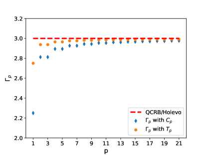
Figure 1: Upper bounds on $\Gamma_{p}$ obtained with $C_{p}$ and $T_{p}$, together with the QCRB/Holevo bound at the case $\delta=0$.

We also plot the bounds for the state $\rho_{x}=\frac{1}{2}(I+\delta\sigma_{3}+x_{1}\sigma_{1}+x_{2}\sigma_{2}+x_{3}\sigma_{3})$ with general $\delta$ in Fig. 2. The complexity of calculating the bound with $C_{p}$, which we compute up to $p=10$, increases exponentially with $p$. As a comparison, the bound with $T_{p}$ is much easier to compute, which we compute up to $p=100$. Since the difference between these two bounds decreases with $p$, a good strategy is to use the bound with $C_{p}$ for small $p$ and use the bound with $T_{p}$ for large $p$. We also plot the bound with the RLD for $p=2$, it can be seen that the RLD bound can be either tighter or less tight than the bound with $C_{p}$. We can combine these bounds and choose the minimal of them to get a tighter bound.

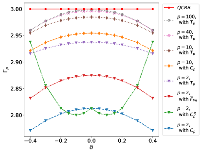
Figure 2: Comparison of different bounds of $\Gamma_{p}$ for the estimation of $\rho_{x}=\frac{1}{2}(I+\delta\sigma_{3}+x_{1}\sigma_{1}+x_{2}\sigma_{2}+x_{3}\sigma_{3})$ at $x_{1}=x_{2}=x_{3}=0$.

VI.2 Example 2

We consider another example with a three dimensional state, $\rho_{x}=\frac{1}{3}I+\sum_{j}x_{j}G_{j}$, where $G_{j}=\frac{1}{2}\Lambda_{j}$, here $\{\Lambda_{j}\}_{j=1}^{8}$ are the Gell-Mann matrices,

$$\Lambda_{1}=\begin{pmatrix}0&1&0\\ 1&0&0\\ 0&0&0\end{pmatrix},\Lambda_{2}=\begin{pmatrix}0&-i&0\\ i&0&0\\ 0&0&0\end{pmatrix},\Lambda_{3}=\begin{pmatrix}1&0&0\\ 0&-1&0\\ 0&0&0\end{pmatrix},$$ (148)

$$\Lambda_{4}=\begin{pmatrix}0&0&1\\ 0&0&0\\ 1&0&0\end{pmatrix},\Lambda_{5}=\begin{pmatrix}0&0&-i\\ 0&0&0\\ i&0&0\end{pmatrix},\Lambda_{6}=\begin{pmatrix}0&0&0\\ 0&0&1\\ 0&1&0\end{pmatrix},$$

$$\Lambda_{7}=\begin{pmatrix}0&0&0\\ 0&0&-i\\ 0&i&0\end{pmatrix},\Lambda_{8}=\frac{1}{\sqrt{3}}\begin{pmatrix}1&0&0\\ 0&1&0\\ 0&0&-2\end{pmatrix},$$

which form a basis for 3 by 3 Hermitian matrices. When the true values of the parameters are all 0, the SLDs can be obtained as $L_{j}=3G_{j}$, and $F_{Q}=\frac{3}{2}I$. The SLDs after the reparametrization which makes $\tilde{F}_{Q}=I$ are given by $\tilde{L}_{j}=\sqrt{\frac{2}{3}}L_{j}=\sqrt{6}G_{j}$. Since

$$(C_{1})_{jk}=\frac{1}{2}\|\sqrt{\rho_{x}}[\tilde{L}_{j},\tilde{L}_{k}]\sqrt{\rho_{x}}\|_{1}=\|[G_{j},G_{k}]\|_{1},$$ (149)

we have

$$C_{1}=\begin{pmatrix}0&1&1&\frac{1}{2}&\frac{1}{2}&\frac{1}{2}&\frac{1}{2}&0\\ 1&0&1&\frac{1}{2}&\frac{1}{2}&\frac{1}{2}&\frac{1}{2}&0\\ 1&1&0&\frac{1}{2}&\frac{1}{2}&\frac{1}{2}&\frac{1}{2}&0\\ \frac{1}{2}&\frac{1}{2}&\frac{1}{2}&0&1&\frac{1}{2}&\frac{1}{2}&\frac{\sqrt{3}}{2}\\ \frac{1}{2}&\frac{1}{2}&\frac{1}{2}&1&0&\frac{1}{2}&\frac{1}{2}&\frac{\sqrt{3}}{2}\\ \frac{1}{2}&\frac{1}{2}&\frac{1}{2}&\frac{1}{2}&\frac{1}{2}&0&1&\frac{\sqrt{3}}{2}\\ \frac{1}{2}&\frac{1}{2}&\frac{1}{2}&\frac{1}{2}&\frac{1}{2}&1&0&\frac{\sqrt{3}}{2}\\ 0&0&0&\frac{\sqrt{3}}{2}&\frac{\sqrt{3}}{2}&\frac{\sqrt{3}}{2}&\frac{\sqrt{3}}{2}&0\end{pmatrix}.$$ (150)

This gives the tradeoff relation under the 1-local measurement as

$$\frac{1}{\nu}Tr[F_{Q}^{-1}Cov^{-1}(\hat{x})] \leq n-\frac{1}{4(n-1)}\|C_{1}\|_{F}^{2}$$ (151)

$$=\frac{50}{7}\approx 7.14.$$

For $p$-local measurement, we can similarly obtain

$$(C_{p})_{jk}=\frac{1}{2}\|\sqrt{\rho_{x}^{\otimes p}}[\tilde{L}_{jp},\tilde{L}_{kp}]\sqrt{\rho_{x}^{\otimes p}}\|_{1}=\frac{1}{3^{p-1}}\|[G_{jp},G_{kp}]\|_{1},$$ (152)

where $[G_{jp},G_{kp}]=\sum_{r=1}^{p}[G_{j}^{(r)},G_{k}^{(r)}]$. Since the eigenvalues of $[G_{j},G_{k}]$ are $\{-\lambda,0,\lambda\}$, where $\lambda=\frac{1}{2}(C_{1})_{jk}$, the eigenvalues of $[G_{jp},G_{kp}]$ are given by $\lambda s$ with multiplicity $\binom{p}{s}_{2}$, for $s=-p,-p+1,\cdots,p$, here $\binom{p}{s}_{2}=\sum_{i=0}^{p}(-1)^{i}\binom{p}{i}\binom{2p-2i}{p-s-i}$ is the trinomial coefficient, which can be obtained as the $(j+p)$-th coefficient of the polynomial $(1+x+x^{2})^{p}$ (see appendix for details). We thus have

$$\begin{aligned} \|[G_{jp},G_{kp}]\|_{1}&=\sum_{s=-p}^{p}|\lambda s|\binom{p}{s}_{2}=2\lambda\sum_{s=0}^{p}s\binom{p}{s}_{2}\\ &=(C_{1})_{jk}\sum_{s=0}^{p}s\binom{p}{s}_{2},\end{aligned}$$ (153)

where we have used the fact that $\binom{p}{s}_{2}=\binom{p}{-s}_{2}$. Denote $\mathcal{N}_{p}=\sum_{s=0}^{p}s\binom{p}{s}_{2}$, we then have

$$(C_{p})_{jk}=\frac{1}{3^{p-1}}\|[G_{jp},G_{kp}]\|_{1}=(C_{1})_{jk}\frac{\mathcal{N}_{p}}{3^{p-1}},$$ (154)

which gives the Frobenius norm of $C_{p}$ as

$$\|C_{p}\|_{F} =\sqrt{\sum_{jk}(C_{p})_{jk}^{2}}=\sqrt{\sum_{jk}\left((C_{1})_{jk}\frac{1}{3^{p-1}}\mathcal{N}_{p}\right)^{2}}$$ (155)

$$=\frac{1}{3^{p-1}}\mathcal{N}_{p}\sqrt{\sum_{jk}\left((C_{1})_{jk}\right)^{2}}=\frac{1}{3^{p-1}}\mathcal{N}_{p}\|C_{1}\|_{F}.$$

The tradeoff relation under the $p$-local measurement is then given by

$$\frac{1}{\nu}Tr[F_{Q}^{-1}Cov^{-1}(\hat{x})] \leq n-\frac{1}{4(n-1)}\|\frac{C_{p}}{p}\|_{F}^{2}$$ (156)

$$=n-\frac{1}{4(n-1)}\|C_{1}\|_{F}^{2}\left(\frac{1}{p3^{p-1}}\mathcal{N}_{p}\right)^{2}$$

$$=8-\frac{6}{7}\left(\frac{1}{p3^{p-1}}\mathcal{N}_{p}\right)^{2}.$$

Here $\frac{1}{p3^{p-1}}\mathcal{N}_{p}$ monotonically decreases with $p$ and it is only equal to $0$ when $p\rightarrow\infty$. The Holevo bound, which equals to the QCRB in this case since the weak commutative condition holds, can thus only be achieved with collective measurement on genuinely infinite number of quantum states in this case.

If there are only three parameters, for example, $\{x_{1},x_{2},x_{5}\}$, the associated matrices are given by the $3\times 3$ submatrices of the original ones. Under the 1-local measurement we have

$$C_{1}=\begin{pmatrix}0&1&\frac{1}{2}\\ 1&0&\frac{1}{2}\\ \frac{1}{2}&\frac{1}{2}&0\end{pmatrix},$$ (157)

which gives the tradeoff relation

$$\begin{aligned} \frac{1}{\nu}Tr[F_{Q}^{-1}Cov(\hat{x})^{-1}]&\leq n-\frac{1}{4(n-1)}\|C_{1}\|_{F}^{2}\\ &=3-\frac{3}{8}=2.625.\end{aligned}$$ (158)

Under the $p$-local measurement, we have

$$\frac{1}{\nu}Tr[F_{Q}^{-1}Cov(\hat{x})^{-1}] \leq n-\frac{1}{4(n-1)}\|\frac{C_{p}}{p}\|_{F}^{2}$$ (159)

$$=n-\frac{1}{4(n-1)}\|C_{1}\|_{F}^{2}\left(\frac{1}{p3^{p-1}}\mathcal{N}_{p}\right)^{2}$$

$$=3-\frac{3}{8}\left(\frac{1}{p3^{p-1}}\mathcal{N}_{p}\right)^{2}.$$

For $p=2$, this gives

$$\begin{aligned} \frac{1}{\nu}Tr[F_{Q}^{-1}Cov(\hat{x})^{-1}]&\leq n-\frac{1}{4(n-1)}\|\frac{C_{2}}{2}\|_{F}^{2}\\ &=3-\frac{3}{8}\times\frac{1}{4}\times\frac{16}{9}\\ &=\frac{17}{6}\approx 2.83.\end{aligned}$$ (160)

The bound with $T_{p}$ can be similarly calculated as $(T_{p})_{jk}=\frac{1}{2}\sum_{s=0}^{p}\sum_{r=0}^{p-s}\binom{p}{s}\binom{p-s}{r}\left(\frac{1+3\delta}{3}\right)^{s}\left(\frac{1-3\delta}{3}\right)^{r}\left(\frac{1}{3}\right)^{p-s-r}|s\times\langle 0|[\tilde{L}_{j},\tilde{L}_{k}]|0\rangle+r\times\langle 1|[\tilde{L}_{j},\tilde{L}_{k}]|1\rangle+(p-s-r)\times\langle 2|[\tilde{L}_{j},\tilde{L}_{k}]|2\rangle|$. For $\delta=0$, the equation can be simplified as

$$(T_{p})_{12}=\frac{1}{2}\left(\frac{1}{3}\right)^{p}\sum_{s=0}^{p}\sum_{r=0}^{p-s}\binom{p}{s}\binom{p-s}{r}|3s-3r|$$ (161)

and $(T_{p})_{13}=0$, $(T_{p})_{23}=0$. This then gives

$$\begin{aligned} \frac{1}{\nu}Tr[F_{Q}^{-1}Cov^{-1}(\hat{x})]&\leq n-\frac{1}{4(n-1)}\|\frac{T_{p}}{p}\|_{F}^{2}\\ &=3-\frac{1}{4p^{2}}(T_{p})_{12}^{2}.\end{aligned}$$ (162)

We plot the bounds for $n=3$ as a typical case in Fig3. It can be seen that the Holevo bound, which equals to the QCRB as the weak commutative condition holds, is only achievable when $p\rightarrow\infty$. For any finite $p$, the bounds are strictly less than $n$.

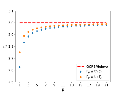
Figure 3: Precision bounds $\Gamma_{p}$ for $p$-local measurements and the Holevo bound when $n=3$.

If there are only two parameters, the associated matrices are then given by the $2\times 2$ submatrices of the original ones. For example, suppose the two parameters are $\{x_{1},x_{2}\}$, we then have

$$C_{1}=\begin{pmatrix}0&1\\ 1&0\end{pmatrix}$$ (163)

the tradeoff relation under the 1-local measurement is then given by

$$\frac{1}{\nu}Tr[F_{Q}^{-1}Cov(\hat{x})^{-1}]\leq n-\frac{1}{4(n-1)}\|C_{1}\|_{F}^{2}=\frac{3}{2},$$ (164)

in this case it is tighter than the Gill-Massar bound .

Under general $p$-local measurement, we have

$$\frac{1}{\nu}Tr[F_{Q}^{-1}Cov(\hat{x})^{-1}] \leq n-\frac{1}{4(n-1)}\|\frac{C_{p}}{p}\|_{F}^{2}$$ (165)

$$=n-\frac{1}{4(n-1)}\|C_{1}\|_{F}^{2}\left(\frac{1}{p3^{p-1}}\mathcal{N}_{p}\right)^{2}$$

$$=2-\frac{1}{2}\left(\frac{1}{p3^{p-1}}\mathcal{N}_{p}\right)^{2}.$$

For $p=2$, we have

$$\frac{1}{\nu}Tr[F_{Q}^{-1}Cov(\hat{x})^{-1}]\leq\frac{16}{9}\approx 1.78,$$ (166)

and for $p=3$,

$$\frac{1}{\nu}Tr[F_{Q}^{-1}Cov(\hat{x})^{-1}]\leq\frac{299}{162}\approx 1.85.$$ (167)

Similar as the previous example, we also consider the estimation of the state $\rho_{x}=\frac{1}{3}I+\delta G_{3}+x_{1}G_{1}+x_{2}G_{2}+x_{5}G_{5}$ with general $\delta$ and plot the precision bounds in Fig. 4, where we plotted the bounds with $C_{p}$ up to $p=6$ and the bounds with $T_{p}$ up to $p=100$. We also plotted the bounds with RLDs and $\mathbf{\bar{F}}_{Im}$ for $p=2$(see appendix for detailed calculations), as it can be seen the bound given by $\frac{1}{\nu}Tr[F_{Q}^{-1}Cov(\hat{x})^{-1}]\leq n-\frac{(n-2)}{(n-1)^{2}}\|\frac{\bar{F}_{Im2}}{2}\|_{F}^{2}$ is tighter than the bounds given by $C_{2}$ and $T_{2}$ in this case.

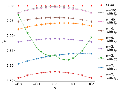
Figure 4: Comparison of different bounds of $\Gamma_{p}$ for the estimation of $\rho_{x}=\frac{1}{3}I+\delta G_{3}+x_{1}G_{1}+x_{2}G_{2}+x_{5}G_{5}$ at $x_{1}=x_{2}=x_{5}=0$.

VII Summary

The presented framework provided a versatile tool to obtain bounds on the precision limit in multi-parameter quantum estimation under general $p$-local measurements, which significantly increased our knowledge on the incompatibility in multi-parameter quantum estimation. The relation between the partial commutative condition and the weak commutative condition is also clarified. Future studies includes improving the bounds by exploring different choices of $\{|u_{q}\rangle\}$ and operators in $\mathbf{\bar{S}}$, clarifying whether the partial commutative condition is sufficient for the saturation of the QCRB, and identifying the ultimate precision under general $p$-local measurements. The approach can also be used to strengthen the uncertainty relations for multiple observables, which is another interesting directions to pursue.

Appendix A Tradeoff Relations

We derive the tradeoff relation from

$$S=\left(\begin{array}[]{cc}A&B\\ B^{\dagger}&F\\ \end{array}\right)\geq 0,$$ (168)

where $A,B,F$ are $n\times n$ matrices with $Cov(\hat{x})\geq A$, $B=I+iB_{Im}$ and $F=F_{Q}+iF_{Im}$. We note that the derivation below works regardless whether $S$ is obtained from pure states or mixed states.

Since $Cov(\hat{x})\geq A$, we have

$$\left(\begin{array}[]{cc}Cov(\hat{x})&B\\ B^{\dagger}&F\\ \end{array}\right)=\left(\begin{array}[]{cc}Cov(\hat{x})-A&0\\ 0&0\\ \end{array}\right)+\left(\begin{array}[]{cc}A&B\\ B^{\dagger}&F\\ \end{array}\right)\geq 0.$$ (169)

This implies that $F-B^{\dagger}Cov^{-1}(\hat{x})B\geq 0$. Since $F=F_{Q}+iF_{Im}$, $B=I+iB_{Im}$, we thus have

$$F_{Q}+iF_{Im}-[Cov^{-1}(\hat{x})+B_{Im}^{T}Cov^{-1}(\hat{x})B_{Im}+i(B_{Im}^{T}Cov^{-1}(\hat{x})-Cov^{-1}(\hat{x})B_{Im})]\geq 0,$$ (170)

which implies the real part is positive semidefinite, i.e.,

$$F_{Q}-Cov^{-1}(\hat{x})-B_{Im}^{T}Cov^{-1}(\hat{x})B_{Im}\geq 0.$$ (171)

This can be written as $F_{Q}-Cov^{-1}(\hat{x})\geq B_{Im}^{T}Cov^{-1}(\hat{x})B_{Im}\geq 0$, which is stronger than the quantum Cramer-Rao bound $F_{Q}-Cov^{-1}(\hat{x})\geq 0$, typically written as $Cov(\hat{x})\geq F_{Q}^{-1}$. To saturate the bound, i.e., $Cov(\hat{x})=F_{Q}^{-1}$, we need to have $B_{Im}^{T}Cov(\hat{x})^{-1}B_{Im}=0$. When the covariance matrix is full rank, which is always the case when $F_{Q}$ is invertable, this requires $B_{Im}=0$, Eq.(170) then becomes

$$F_{Q}+iF_{Im}-Cov^{-1}(\hat{x})\geq 0.$$ (172)

The saturation of the quantum Cramer-Rao bound then requires $iF_{Im}\geq 0$. Since $F_{Im}$ is anti-symmetric and its eigenvalues are in the form of $\pm i\beta$ with $\beta\in\mathbb{R}$, $iF_{Im}\geq 0$ is only possible when all the eigenvalues are zero, i.e., $F_{Im}=0$. This is exactly the weak commutative condition for the saturation of the quantum Cramer-Rao bound.

When $F_{Im}\neq 0$, the QCRB is not saturable. Denote $F_{C}=Cov^{-1}(\hat{x})$, we write Eq.(170) as

$$F_{Q}-F_{C}-B_{Im}^{T}F_{C}B_{Im}+i(F_{Im}+B_{Im}^{T}F_{C}-F_{C}B_{Im})]\geq 0.$$ (173)

By multiplying $F_{Q}^{-\frac{1}{2}}$ from both the left and the right, we get

$$I-F_{Q}^{-\frac{1}{2}}F_{C}F_{Q}^{-\frac{1}{2}}-F_{Q}^{-\frac{1}{2}}B_{Im}^{T}F_{C}B_{Im}F_{Q}^{-\frac{1}{2}}+i(F_{Q}^{-\frac{1}{2}}F_{Im}F_{Q}^{-\frac{1}{2}}+F_{Q}^{-\frac{1}{2}}B_{Im}^{T}F_{C}F_{Q}^{-\frac{1}{2}}-F_{Q}^{-\frac{1}{2}}F_{C}B_{Im}F_{Q}^{-\frac{1}{2}})]\geq 0.$$ (174)

Denote $\tilde{F}_{C}=F_{Q}^{-\frac{1}{2}}F_{C}F_{Q}^{-\frac{1}{2}}$, $\tilde{B}_{Im}=F_{Q}^{\frac{1}{2}}B_{Im}F_{Q}^{-\frac{1}{2}}$, $\tilde{F}_{Im}=F_{Q}^{-\frac{1}{2}}F_{Im}F_{Q}^{-\frac{1}{2}}$, we can write the inequality as

$$I-\tilde{F}_{C}-\tilde{B}_{Im}^{T}\tilde{F}_{C}\tilde{B}_{Im}+i(\tilde{F}_{Im}+\tilde{B}_{Im}^{T}\tilde{F}_{C}-\tilde{F}_{C}\tilde{B}_{Im}]\geq 0.$$ (175)

Since $F_{C}\leq F_{Q}$, we have $\tilde{F}_{C}\leq I$, thus $\tilde{F}_{C}\geq\tilde{F}_{C}^{2}$ and $\tilde{B}_{Im}^{T}\tilde{F}_{C}\tilde{B}_{Im}\geq\tilde{B}_{Im}^{T}\tilde{F}_{C}^{2}\tilde{B}_{Im}$. We then have

$$I-\tilde{F}_{C}-\tilde{B}_{Im}^{T}\tilde{F}_{C}^{2}\tilde{B}_{Im}+i(\tilde{F}_{Im}+\tilde{B}_{Im}^{T}\tilde{F}_{C}-\tilde{F}_{C}\tilde{B}_{Im}]\geq 0.$$ (176)

Now denote $\tilde{F}_{C}\tilde{B}_{Im}$ as $D$,

$$I-\tilde{F}_{C}-D^{T}D+i(\tilde{F}_{Im}+D^{T}-D)\geq 0.$$ (177)

Since any two by two principle submatrix of a positive semidefinite matrix is also positive semidefinite,

$$\begin{aligned} \left(\begin{array}[]{cc}1-(\tilde{F}_{C})_{jj}-(D^{T}D)_{jj}&-(\tilde{F}_{C})_{jk}-(D^{T}D)_{jk}\\ -(\tilde{F}_{C})_{kj}-(D^{T}D)_{kj}&1-(\tilde{F}_{C})_{kk}-(D^{T}D)_{kk}\\ \end{array}\right)&+i\left(\begin{array}[]{cc}0&(\tilde{F}_{Im})_{jk}+D_{kj}-D_{jk}\\ -(\tilde{F}_{Im})_{jk}-D_{kj}+D_{jk}&0\\ \end{array}\right)\end{aligned}$$ (178)

is then positive semidefinite. Note that $\tilde{F}_{C}$ and $D^{T}D$ are symmetric and the determination of a positive semidefinite matrix is nonnegative, we thus have

$$[1-(\tilde{F}_{C})_{jj}-(D^{T}D)_{jj}][1-(\tilde{F}_{C})_{kk}-(D^{T}D)_{kk}]\geq[(\tilde{F}_{C})_{jk}+(D^{T}D)_{jk}]^{2}+[(\tilde{F}_{Im})_{jk}+D_{kj}-D_{jk}]^{2},$$ (179)

from which we can get

$$\begin{aligned} &[1-(\tilde{F}_{C})_{jj}-(D^{T}D)_{jj}]+[1-(\tilde{F}_{C})_{kk}-(D^{T}D)_{kk}]\\ &\geq 2\sqrt{[1-(\tilde{F}_{C})_{jj}-(D^{T}D)_{jj}][1-(\tilde{F}_{C})_{kk}-(D^{T}D)_{kk}]}\\ &\geq 2\sqrt{[(\tilde{F}_{C})_{jk}+(D^{T}D)_{jk}]^{2}+[(\tilde{F}_{Im})_{jk}+D_{kj}-D_{jk}]^{2}}\\ &\geq 2|(\tilde{F}_{Im})_{jk}+D_{kj}-D_{jk}|,\end{aligned}$$ (180)

i.e.,

$$1-(\tilde{F}_{C})_{jj}+1-(\tilde{F}_{C})_{kk}\geq 2|(\tilde{F}_{Im})_{jk}+D_{kj}-D_{jk}|+(D^{T}D)_{jj}+(D^{T}D)_{kk}.$$ (181)

As $(D^{T}D)_{jj}=\sum_{p}D_{pj}^{2}\geq D_{kj}^{2}$ and $(D^{T}D)_{kk}=\sum_{p}D_{pk}^{2}\geq D_{jk}^{2}$, we have

$$(D^{T}D)_{jj}+(D^{T}D)_{kk}=\sum_{p}(D_{pj}^{2}+D_{pk}^{2})\geq D_{kj}^{2}+D_{jk}^{2}=\frac{1}{2}(D_{kj}-D_{jk})^{2}+\frac{1}{2}(D_{kj}+D_{jk})^{2},$$ (182)

and from $I+i\tilde{F}_{Im}=F_{Q}^{-\frac{1}{2}}FF_{Q}^{-\frac{1}{2}}\geq 0$, we have $|(\tilde{F}_{Im})_{jk}|\leq 1$. Thus

$$\begin{aligned} 1-(\tilde{F}_{C})_{jj}+1-(\tilde{F}_{C})_{kk}&\geq 2|(\tilde{F}_{Im})_{jk}+D_{kj}-D_{jk}|+(D^{T}D)_{jj}+(D^{T}D)_{kk}\\ &\geq 2|(\tilde{F}_{Im})_{jk}+D_{kj}-D_{jk}|+\frac{1}{2}(D_{kj}-D_{jk})^{2}\\ &\geq\frac{1}{2}|(\tilde{F}_{Im})_{jk}|^{2},\end{aligned}$$ (183)

where the last inequality we used the fact that $2|y+x|+\frac{1}{2}x^{2}\geq\frac{1}{2}y^{2}$ when $|y|\leq 1$, since

$$\begin{aligned} 2|y+x|+\frac{1}{2}x^{2}&=2|y+x|+\frac{1}{2}(y+x-y)^{2}\\ &=2|y+x|+\frac{1}{2}(y+x)^{2}-y(x+y)+\frac{1}{2}y^{2}\\ &\geq 2|y+x|-|y(x+y)|+\frac{1}{2}y^{2}\\ &=(2-|y|)|x+y|+\frac{1}{2}y^{2}\\ &\geq\frac{1}{2}y^{2}.\end{aligned}$$ (184)

This provides a tradeoff relation between $(\tilde{F}_{C})_{jj}$ and $(\tilde{F}_{C})_{kk}$. When $F_{Im}=0$, the quantum Cramér-Rao bound is saturable, $F_{C}$ can reach $F_{Q}$, in this case $\tilde{F}_{C}=I$, $(\tilde{F}_{C})_{jj}$ and $(\tilde{F}_{C})_{kk}$ can reach the maximal value simultaneously, which is 1. When $(\tilde{F}_{Im})_{jk}\neq 0$, $(\tilde{F}_{C})_{jj}$ and $(\tilde{F}_{C})_{kk}$ can not simultaneously reach 1, Eq.(183) puts a tradeoff between them.

By summing Eq.(183) over different choice of $j,k$ directly, we can get

$$2(n-1)\sum_{j}[1-(\tilde{F}_{C})_{jj}]\geq\frac{1}{2}\sum_{j,k,j\neq k}|(\tilde{F}_{Im})_{jk}|^{2}=\frac{1}{2}\|\tilde{F}_{Im}\|_{F}^{2},$$ (185)

which gives

$$Tr(\tilde{F}_{C})\leq n-\frac{1}{4(n-1)}\|\tilde{F}_{Im}\|_{F}^{2}.$$ (186)

where $\|\tilde{F}_{Im}\|_{F}^{2}=Tr(\tilde{F}_{Im}^{T}\tilde{F}_{Im})$. This can be rewritten as

$$\begin{aligned} Tr[F_{Q}^{-1}Cov^{-1}(\hat{x})]&\leq n-\frac{1}{4(n-1)}\|F_{Q}^{-\frac{1}{2}}F_{Im}F_{Q}^{-\frac{1}{2}}\|_{F}^{2}\\ &=n-\frac{1}{4(n-1)}Tr(F_{Q}^{-1}F_{Im}^{T}F_{Q}^{-1}F_{Im}),\end{aligned}$$ (187)

The same relation can be obtained by including the number of copies of the state, $\nu$, explicitly, essentially just replace $F_{Q}$ and $F_{Im}$ with $\nu F_{Q}$ and $\nu F_{Im}$. The tradeoff relation with $\nu$ copies of the state is then

$$\frac{1}{\nu}Tr[F_{Q}^{-1}Cov^{-1}(\hat{x})]\leq n-\frac{1}{4(n-1)}\|F_{Q}^{-\frac{1}{2}}F_{Im}F_{Q}^{-\frac{1}{2}}\|_{F}^{2}.$$ (188)

When the number of the parameters, $n\geq 3$, the tradeoff can be tightened by keeping all terms in $(D^{T}D)_{jj}$ and $(D^{T}D)_{kk}$ in Eq.(181) as

$$\sum_{j,k,j\neq k}[1-(\tilde{F}_{C})_{jj}+1-(\tilde{F}_{C})_{kk}]\geq\sum_{j,k,j\neq k}[2|(\tilde{F}_{Im})_{jk}+D_{kj}-D_{jk}|+(D^{T}D)_{jj}+(D^{T}D)_{kk}],$$ (189)

here

$$(D^{T}D)_{jj}+(D^{T}D)_{kk}=\sum_{p}(D_{pj}^{2}+D_{pk}^{2}),$$ (190)

which not only includes the correlations between the $j,k$-th entry, but also with other entries. By summing over all choice of $j,k$, we have

$$\begin{aligned} 2(n-1)\sum_{j}[1-(\tilde{F}_{C})_{jj}]&\geq\sum_{j,k,j\neq k}2|(\tilde{F}_{Im})_{jk}+D_{kj}-D_{jk}|+2(n-1)\sum_{j}(D^{T}D)_{jj}\\ &=\sum_{j,k,j\neq k}2|(\tilde{F}_{Im})_{jk}+D_{kj}-D_{jk}|+2(n-1)\sum_{j,k}D_{jk}^{2}\\ &\geq\sum_{j,k,j\neq k}\{2|(\tilde{F}_{Im})_{jk}+D_{kj}-D_{jk}|+(n-1)(D_{jk}^{2}+D_{kj}^{2})\}\\ &=\sum_{j,k,j\neq k}\{2|(\tilde{F}_{Im})_{jk}+D_{kj}-D_{jk}|+\frac{n-1}{2}(D_{kj}-D_{jk})^{2}+\frac{n-1}{2}(D_{kj}+D_{jk})^{2}\}\\ &\geq\frac{2(n-2)}{n-1}\sum_{j,k,j\neq k}|(\tilde{F}_{Im})_{jk}|^{2}\\ &=\frac{2(n-2)}{n-1}\|\tilde{F}_{Im}\|_{F}^{2},\end{aligned}$$ (191)

where the last inequality we used the fact that

$$\begin{aligned} 2|y+x|+\frac{n-1}{2}x^{2}&=2|y+x|+\frac{n-1}{2}(y+x-y)^{2}\\ &=2|y+x|+\frac{n-1}{2}(y+x)^{2}-(n-1)y(x+y)+\frac{n-1}{2}y^{2}\\ &\geq\frac{n-1}{2}(y+x)^{2}+2|y||y+x|-(n-1)|y(x+y)|+\frac{n-1}{2}y^{2}\\ &=\frac{n-1}{2}(y+x)^{2}-(n-3)|y||x+y|+\frac{n-1}{2}y^{2}\\ &=\frac{n-1}{2}(|y+x|-\frac{n-3}{n-1}|y|)^{2}+\frac{2(n-2)}{n-1}y^{2}\\ &\geq\frac{2(n-2)}{n-1}y^{2}.\end{aligned}$$ (192)

This then gives a tradeoff relation on $\tilde{F}_{C}$ as

$$Tr(\tilde{F}_{C})\leq n-\frac{n-2}{(n-1)^{2}}\|\tilde{F}_{Im}\|_{F}^{2}.$$ (193)

With $\nu$ copies of the state, this can be equivalently written

$$\frac{1}{\nu}Tr[F_{Q}^{-1}Cov^{-1}(\hat{x})]\leq n-\frac{n-2}{(n-1)^{2}}\|F_{Q}^{-\frac{1}{2}}F_{Im}F_{Q}^{-\frac{1}{2}}\|_{F}^{2}.$$ (194)

The bound can be further improved. From Eq.(177),

$$I-\tilde{F}_{C}-D^{T}D+i(\tilde{F}_{Im}+D^{T}-D)\geq 0,$$ (195)

we have

$$I-\tilde{F}_{C}-D^{T}D\geq-i(\tilde{F}_{Im}+D^{T}-D),$$ (196)

from which we can obtain

$$Tr(I-\tilde{F}_{C}-D^{T}D)\geq\|\tilde{F}_{Im}+D^{T}-D\|_{1}.$$ (197)

Note that $\tilde{F}_{Im}+D^{T}-D$ is skew symmetric with purely imaginary eigenvalues, and the singular values are just the amplitude of the eigenvalues as $\{|\lambda_{1}|,\cdots,|\lambda_{n}|\}$. Since

$$-i(\tilde{F}_{Im}+D^{T}-D)\leq I-\tilde{F}_{C}-D^{T}D\leq I,$$ (198)

we have $|\lambda_{j}|\leq 1$, thus $|\lambda_{j}|\geq|\lambda_{j}|^{2}$. As

$$\begin{aligned} \|\tilde{F}_{Im}+D^{T}-D\|_{1}=\sum_{j=1}^{n}|\lambda_{j}|&\geq\sum_{j=1}^{n}|\lambda_{j}|^{2}\\ &=Tr[(\tilde{F}_{Im}+D^{T}-D)^{T}(\tilde{F}_{Im}+D^{T}-D)]\\ &=\sum_{jk}[(\tilde{F}_{Im}+D^{T}-D)_{jk}]^{2},\end{aligned}$$ (199)

from Eq.(197) we then have

$$\begin{aligned} Tr(I-\tilde{F}_{C})&\geq Tr(D^{T}D)+\|\tilde{F}_{Im}+D^{T}-D\|_{1}\\ &\geq\sum_{k}(D^{T}D)_{kk}+\sum_{jk}[(\tilde{F}_{Im}+D^{T}-D)_{jk}]^{2}\\ &=\sum_{jk}D_{jk}^{2}+[(\tilde{F}_{Im})_{jk}+D_{kj}-D_{jk}]^{2}\\ &=\sum_{jk}\frac{1}{2}(D_{jk}^{2}+D_{kj}^{2})+[(\tilde{F}_{Im})_{jk}+D_{kj}-D_{jk}]^{2}\\ &\geq\sum_{jk}\frac{1}{4}(D_{jk}-D_{kj})^{2}+[(\tilde{F}_{Im})_{jk}+D_{kj}-D_{jk}]^{2}\\ &\geq\sum_{jk}\frac{1}{5}(\tilde{F}_{Im})_{jk}^{2}\\ &=\frac{1}{5}\|\tilde{F}_{Im}\|_{F}^{2},\end{aligned}$$ (200)

where the last inequality we used the fact that

$$\begin{aligned} \frac{1}{4}x^{2}+(y+x)^{2}&=\frac{5}{4}x^{2}+2xy+y^{2}\\ &=\frac{5}{4}(x+\frac{4}{5}y)^{2}+\frac{1}{5}y^{2}\\ &\geq\frac{1}{5}y^{2}.\end{aligned}$$ (201)

We thus have

$$Tr(\tilde{F}_{C})\leq n-\frac{1}{5}\|\tilde{F}_{Im}\|_{F}^{2}.$$ (202)

For $\nu$ copies of the state, this gives the tradeoff relation

$$\frac{1}{\nu}Tr[F_{Q}^{-1}Cov^{-1}(\hat{x})]\leq n-\frac{1}{5}\|F_{Q}^{-\frac{1}{2}}F_{Im}F_{Q}^{-\frac{1}{2}}\|_{F}^{2},$$ (203)

which is tighter than Eq.(193) when $n\geq 5$.

Appendix B Connection between the partial commutative condition and the weak commutative condition

Here we show

$$\lim_{p\rightarrow\infty}\frac{\|\sqrt{\rho_{x}^{\otimes p}}[L_{jp},L_{kp}]\sqrt{\rho_{x}^{\otimes p}}\|_{1}}{p}=|Tr(\rho_{x}[L_{j},L_{k}])|.$$ (204)

We write the state in the eigenvalue decomposition as $\rho_{x}=\sum_{q=1}^{m}\lambda_{q}|\Psi_{q}\rangle\langle\Psi_{q}|$ with $\lambda_{q}>0$ and $\sum_{q=1}^{m}\lambda_{q}=1$. Then $\sqrt{\rho_{x}}=\sum_{q}\sqrt{\lambda_{q}}|\Psi_{q}\rangle\langle\Psi_{q}|$,

$$\begin{aligned} \|\sqrt{\rho_{x}^{\otimes p}}[L_{jp},L_{kp}]\sqrt{\rho_{x}^{\otimes p}}\|_{1}=&\|\sqrt{\rho_{x}^{\otimes p}}\sum_{r=1}^{p}[L_{j}^{(r)},L_{k}^{(r)}]\sqrt{\rho_{x}^{\otimes p}}\|_{1}\\ =&\|\sum_{r=1}^{p}\rho_{x}^{\otimes(r-1)}\otimes(\sqrt{\rho_{x}}[L_{j},L_{k}]\sqrt{\rho_{x}})\otimes\rho_{x}^{\otimes(p-r)}\|_{1},\end{aligned}$$ (205)

here $L_{j}^{(r)}=I^{\otimes(r-1)}\otimes L_{j}\otimes I^{\otimes(p-r)}$. The support of $\sum_{r=1}^{p}\rho_{x}^{\otimes(r-1)}\otimes(\sqrt{\rho_{x}}[L_{j},L_{k}]\sqrt{\rho_{x}})\otimes\rho_{x}^{\otimes(p-r)}$ is in the subspace spanned by $\{|\Psi_{v_{1}}\Psi_{v_{2}}\cdots\Psi_{v_{p}}\rangle\}$, with $|\Psi_{v_{1}}\rangle,\cdots,|\Psi_{v_{p}}\rangle\in\{|\Psi_{1}\rangle,\cdots,|\Psi_{m}\rangle\}$, here $\{|\Psi_{1}\rangle,\cdots,|\Psi_{m}\rangle\}$ are the eigenvectors of $\rho_{x}$ with nonzero eigenvalues. We can focus on the support space and calculate the entries of $\sum_{r=1}^{p}\rho_{x}^{\otimes(r-1)}\otimes\sqrt{\rho_{x}}[L_{j},L_{k}]\sqrt{\rho_{x}}\otimes\rho_{x}^{\otimes(p-r)}$ in the basis of $|\Psi_{v_{1}}\Psi_{v_{2}}\cdots\Psi_{v_{p}}\rangle$ with $v_{1},\cdots,v_{p}\in\{1,\cdots,m\}$ and show that when $p\rightarrow\infty$, $\frac{\|\sqrt{\rho_{x}^{\otimes p}}[L_{jp},L_{kp}]|\sqrt{\rho_{x}^{\otimes p}}\|_{1}}{p}\rightarrow|Tr(\rho_{x}[L_{j},L_{k}])|$.

The entries of $\sqrt{\rho_{x}^{\otimes p}}[L_{jp},L_{kp}]|\sqrt{\rho_{x}^{\otimes p}}$ is given by

$$\begin{aligned} &\langle\Psi_{\tilde{v}_{1}}\cdots\Psi_{\tilde{v}_{p}}|\sum_{r=1}^{p}\rho_{x}^{\otimes(r-1)}\otimes\sqrt{\rho_{x}}[L_{j},L_{k}]\sqrt{\rho_{x}}\otimes\rho_{x}^{\otimes(p-r)}|\Psi_{v_{1}}\cdots\Psi_{v_{p}}\rangle\\ &=\sum_{r=1}^{p}[\langle\Psi_{\tilde{v}_{r}}|\sqrt{\rho_{x}}[L_{j},L_{k}]\sqrt{\rho_{x}}|\Psi_{v_{r}}\rangle\prod_{q\neq r}(\delta_{\tilde{v}_{q}}^{v_{q}}\lambda_{v_{q}})].\end{aligned}$$ (206)

It is easy to see that when the indexes $\{v_{1},v_{2}\cdots,v_{p}\}$ and $\{\tilde{v}_{1},\cdots,\tilde{v}_{p}\}$ differ at two or more entries, the corresponding matrix entry equals to 0. When the two indexes differ at only one entry, for example, $v_{r}\neq\tilde{v}_{r}$ but $v_{q}=\tilde{v}_{q}$ for all $q\neq r$, the corresponding matrix entry equals to

$$\begin{aligned} \langle\Psi_{\tilde{v}_{r}}|\sqrt{\rho_{x}}[L_{j},L_{k}]\sqrt{\rho_{x}}|\Psi_{v_{r}}\rangle\prod_{q\neq r}\lambda_{\tilde{v}_{q}}=\frac{\langle\Psi_{\tilde{v}_{r}}|\sqrt{\rho_{x}}[L_{j},L_{k}]\sqrt{\rho_{x}}|\Psi_{v_{r}}\rangle}{\lambda_{\tilde{v}_{r}}}\prod_{q=1}^{p}\lambda_{\tilde{v}_{q}}.\end{aligned}$$ (207)

When the indexes $\{v_{1},v_{2}\cdots,v_{p}\}$ and $\{\tilde{v}_{1},\cdots,\tilde{v}_{p}\}$ are the same, we get the diagonal entries of $\sqrt{\rho_{x}^{\otimes p}}[L_{jp},L_{kp}]|\sqrt{\rho_{x}^{\otimes p}}$ as

$$\begin{aligned} \sum_{r=1}^{p}(\langle\Psi_{v_{r}}|\sqrt{\rho_{x}}[L_{j},L_{k}]\sqrt{\rho_{x}}|\Psi_{v_{r}}\rangle\prod_{q\neq r}\lambda_{v_{q}})&=\sum_{r=1}^{p}(\langle\Psi_{v_{r}}|[L_{j},L_{k}]|\Psi_{v_{r}}\rangle\prod_{q=1}^{p}\lambda_{v_{q}})\\ &=(\prod_{q=1}^{p}\lambda_{v_{q}})\sum_{r=1}^{p}\langle\Psi_{v_{r}}|[L_{j},L_{k}]|\Psi_{v_{r}}\rangle.\end{aligned}$$ (208)

Next we write $\sqrt{\rho_{x}^{\otimes p}}[L_{jp},L_{kp}]|\sqrt{\rho_{x}^{\otimes p}}=D_{p}^{(jk)}+O_{p}^{(jk)}$ with $D_{p}^{(jk)}$ as the diagonal part of the matrix and $O_{p}^{(jk)}$ as the off-diagonal part of the matrix. We then use the inequality

$$\|D_{p}^{(jk)}\|_{1}\leq\|D_{p}^{(jk)}+O_{p}^{(jk)}\|_{1}\leq\|D_{p}^{(jk)}\|_{1}+\|O_{p}^{(jk)}\|_{1}$$ (209)

to bound $\|\sqrt{\rho_{x}^{\otimes p}}[L_{jp},L_{kp}]|\sqrt{\rho_{x}^{\otimes p}}\|_{1}$, here the first inequality comes from the fact that for any matrix, $M$, $\|M\|_{1}\geq\sum_{q}|M_{qq}|$, and for diagonal matrix $\|D_{p}^{(jk)}\|_{1}=\sum_{q}|(D_{p}^{(jk)})_{qq}|$, the second inequality is from the triangle inequality of the trace norm.

The singular values of the diagonal matrix, $D_{p}^{(jk)}$, are just the absolute value of the diagonal entries, which are $\{(\prod_{r=1}^{p}\lambda_{v_{r}})|\sum_{r=1}^{p}\langle\Psi_{v_{r}}|[L_{j},L_{k}]|\Psi_{v_{r}}\rangle|\}$. These entries can be interpreted as the absolute value of the summation of $p$ randomly chosen $\langle\Psi_{v_{r}}|[L_{j},L_{k}]|\Psi_{v_{r}}\rangle$ multiplied with the corresponding probabilities, where each term $\langle\Psi_{v_{r}}|[L_{j},L_{k}]|\Psi_{v_{r}}\rangle$ is selected with probability $\lambda_{v_{r}}$. For a given diagonal entry with a particular choice of $p$ terms, $|\sum_{r=1}^{p}\langle\Psi_{v_{r}}|[L_{j},L_{k}]|\Psi_{v_{r}}\rangle|$, the associated probability is $\prod_{r=1}^{p}\lambda_{v_{r}}$. $\|D_{p}^{(jk)}\|_{1}$, which equals to the summation of the absolute value of all diagonal entries, then corresponds to the expected value of $|\sum_{r=1}^{p}\langle\Psi_{v_{r}}|[L_{j},L_{k}]|\Psi_{v_{r}}\rangle|$ with each $|\Psi_{v_{r}}\rangle$ selected with probability $\lambda_{v_{r}}$. When $p\rightarrow\infty$, by the law of large numbers, $\frac{\sum_{r=1}^{p}\langle\Psi_{v_{r}}|[L_{j},L_{k}]|\Psi_{v_{r}}\rangle}{p}$ converges to the expected value of $\langle\Psi_{v_{r}}|[L_{j},L_{k}]|\Psi_{v_{r}}\rangle$ with probability one, i.e., with probability one

$$\begin{aligned} \frac{\sum_{r=1}^{p}\langle\Psi_{v_{r}}|[L_{j},L_{k}]|\Psi_{v_{r}}\rangle}{p}&\rightarrow E[\langle\Psi_{v_{r}}|[L_{j},L_{k}]|\Psi_{v_{r}}\rangle]\\ &=\sum_{q=1}^{m}\lambda_{q}\langle\Psi_{q}|[L_{j},L_{k}]|\Psi_{q}\rangle\\ &=\sum_{q=1}^{m}\lambda_{q}Tr(|\Psi_{q}\rangle\langle\Psi_{q}|[L_{j},L_{k}])\\ &=Tr(\rho_{x}[L_{j},L_{k}]).\end{aligned}$$ (210)

Thus when $p\rightarrow\infty$,

$$\begin{aligned} \|D_{p}^{(jk)}\|_{1}&=E[|\sum_{r=1}^{p}\langle\Psi_{v_{r}}|[L_{j},L_{k}]|\Psi_{v_{r}}\rangle|]\\ &\rightarrow 1\times|E[\sum_{r=1}^{p}\langle\Psi_{v_{r}}|[L_{j},L_{k}]|\Psi_{v_{r}}\rangle]|\\ &=p|Tr(\rho_{x}[L_{j},L_{k}])|.\end{aligned}$$ (211)

For the off-diagonal part, note that for any matrix, we have $\|M\|_{1}\leq\sum_{j}\sqrt{\sum_{k}|M_{jk}|^{2}}$, and

$$\begin{aligned} &|\frac{\langle\Psi_{\tilde{v}_{r}}|\sqrt{\rho_{x}}[L_{j},L_{k}]\sqrt{\rho_{x}}|\Psi_{v_{r}}\rangle}{\lambda_{\tilde{v}_{r}}}\prod_{q=1}^{p}\lambda_{\tilde{v}_{q}}|\leq&l_{\max}\prod_{q=1}^{p}\lambda_{\tilde{v}_{q}},\end{aligned}$$ (212)

here $l_{\max}=\max_{\tilde{v}_{r}\neq v_{r}}\{|\frac{\langle\Psi_{\tilde{v}_{r}}|\sqrt{\rho_{x}}[L_{j},L_{k}]\sqrt{\rho_{x}}|\Psi_{v_{r}}\rangle}{\lambda_{\tilde{v}_{r}}}|\}$, we then have

$$\begin{aligned} \|O_{p}^{(jk)}\|_{1}&\leq\sum_{\tilde{v}_{1},\cdots,\tilde{v}_{p}}\sqrt{\sum_{r=1}^{p}\sum_{v_{r}\neq\tilde{v}_{r}}l_{\max}^{2}\prod_{q=1}^{p}\lambda^{2}_{\tilde{v}_{q}}}\\ &=\sum_{\tilde{v}_{1},\cdots,\tilde{v}_{p}}\sqrt{p(m-1)l_{\max}^{2}\prod_{q=1}^{p}\lambda^{2}_{\tilde{v}_{q}}}\\ &=\sqrt{(m-1)p}l_{\max}\sum_{\tilde{v}_{1},\cdots,\tilde{v}_{p}}\prod_{q=1}^{p}\lambda_{\tilde{v}_{q}}\\ &=\sqrt{(m-1)p}l_{\max}\prod_{q=1}^{p}(\sum_{\tilde{v}_{q}=1}^{m}\lambda_{\tilde{v}_{q}})\\ &=\sqrt{(m-1)p}l_{\max}.\end{aligned}$$ (213)

Thus when $p\rightarrow\infty$,

$$\begin{aligned} \frac{\|D_{p}^{(jk)}+O_{p}^{(jk)}\|_{1}}{p}&\geq\frac{\|D_{p}^{(jk)}\|_{1}}{p}=|Tr(\rho_{x}[L_{j},L_{k}])|,\\ \frac{\|D_{p}^{(jk)}+O_{p}^{(jk)}\|_{1}}{p}&\leq\frac{\|D_{p}^{(jk)}\|_{1}+\|O_{p}^{(jk)}\|_{1}}{p}\leq|Tr(\rho_{x}[L_{j},L_{k}])|+\frac{\sqrt{(m-1)}l_{\max}}{\sqrt{p}},\end{aligned}$$ (214)

i.e.,

$$\begin{aligned} |Tr(\rho_{x}[L_{j},L_{k}])|\leq\frac{\|\sqrt{\rho_{x}^{\otimes p}}[L_{jp},L_{kp}]|\sqrt{\rho_{x}^{\otimes p}}\|_{1}}{p}\leq|Tr(\rho_{x}[L_{j},L_{k}])|+\frac{\sqrt{(m-1)}l_{\max}}{\sqrt{p}}.\end{aligned}$$ (215)

From which it is easy to see that $\lim_{p\rightarrow\infty}\frac{\|\sqrt{\rho_{x}^{\otimes p}}[L_{jp},L_{kp}]|\sqrt{\rho_{x}^{\otimes p}}\|_{1}}{p}=|Tr(\rho_{x}[L_{j},L_{k}])|$. The condition, $\frac{\|\sqrt{\rho_{x}^{\otimes p}}[L_{jp},L_{kp}]|\sqrt{\rho_{x}^{\otimes p}}\|_{1}}{p}=0$, then reduces to the weak commutative condition, $Tr(\rho_{x}[L_{j},L_{k}])=0$, when $p\rightarrow\infty$.

It can also be seen that $\frac{\|D_{p}^{(jk)}\|_{1}}{p}$ provides a lower bound on $\frac{\|\sqrt{\rho_{x}^{\otimes p}}[L_{jp},L_{kp}]|\sqrt{\rho_{x}^{\otimes p}}\|_{1}}{p}$ and the difference between them is in the order of $O(\frac{1}{\sqrt{p}})$. We can thus use $\|D_{p}^{(jk)}\|_{1}$ to provide an alternative tradeoff relation, which is less tight but easier to compute. Under p-local measurements the tradeoff relation can be written as

$$\frac{1}{\nu}Tr[F_{Q}^{-1}Cov^{-1}(\hat{x})]\leq n-\frac{1}{4(n-1)}\|\frac{T_{p}}{p}\|_{F}^{2},$$ (216)

where

$$\begin{aligned} (T_{p})_{jk}&=\frac{1}{2}\|D_{p}^{(jk)}\|_{1}\\ &=\frac{1}{2}\sum_{v_{1},\cdots,v_{p}}(\prod_{r=1}^{p}\lambda_{v_{r}})|\sum_{r=1}^{p}\langle\Psi_{v_{r}}|[\tilde{L}_{j},\tilde{L}_{k}]|\Psi_{v_{r}}\rangle|,\end{aligned}$$ (217)

where $\tilde{L}_{j}=\sum_{\mu}(F_{Q}^{-{\frac{1}{2}}})_{j\mu}L_{\mu}$ and $\tilde{L}_{k}=\sum_{\mu}(F_{Q}^{-{\frac{1}{2}}})_{k\mu}L_{\mu}$. Compared to $C_{p}$, $T_{p}$ is expressed only with operators on a single copy of the state. We note that $T_{p}$ can be equivalently obtained by choosing the set of $\{|u_{j}\rangle\}$ in Eq.(49) as the eigenvectors of $\rho_{x}$, instead of the eigenvectors of $\sqrt{\rho_{x}}[\tilde{L}_{j},\tilde{L}_{k}]\sqrt{\rho_{x}}$.

Appendix C Bound on the trace norm

For completeness, here we include a proof for the inequality $\sum_{j}|M_{jj}|\leq\|M\|_{1}\leq\sum_{j}\sqrt{\sum_{k}|M_{jk}|^{2}}$, which is used in the derivation that $\frac{C_{p}}{p}=0$ reduces to the weak commutative condition when $p\rightarrow\infty$.

We first show $\|M\|_{1}\leq\sum_{j}\sqrt{\sum_{k}|M_{jk}|^{2}}$.

From the singular value decomposition, $M=U\Lambda V$, we have

$$\begin{aligned} \|M\|_{1}&=Tr(\Lambda)=Tr(U^{\dagger}MV^{\dagger})=Tr(V^{\dagger}U^{\dagger}M)=Tr(WM),\end{aligned}$$ (218)

where $W=V^{\dagger}U^{\dagger}$ is a unitary matrix. Note that

$$\begin{aligned} (WM)_{jj}&=\sqrt{|(WM)_{jj}|^{2}}\leq\sqrt{\sum_{k}|(WM)_{jk}|^{2}}\\ &=\|(WM)_{j}\|_{2}\\ &=\|WM_{j}\|_{2}\\ &=\|M_{j}\|_{2}\\ &=\sqrt{\sum_{k}M^{2}_{jk}},\end{aligned}$$ (219)

where we used $()_{j}$ to denote the $j$-th column of a matrix(thus $(WM)_{j}$ is the $j$-th column of $WM$ which equals to $WM_{j}$, $W$ multiples the $j$-th column of $M$), and $\|v\|_{2}=\sqrt{\sum_{k}|v_{k}|^{2}}$ as the $l_{2}$ norm for a vector. It is then straightforward to see

$$\begin{aligned} \|M\|_{1}&=Tr(WM)=\sum_{j}(WM)_{jj}\leq\sum_{j}\sqrt{\sum_{k}M^{2}_{jk}},\end{aligned}$$ (220)

Next we show $\sum_{j}|M_{jj}|\leq\|M\|_{1}$. From the singular value decomposition, $M=U\Lambda V$, we have

$$M_{jj}=\sum_{k}U_{jk}\Lambda_{kk}V_{kj},$$ (221)

thus

$$\begin{aligned} \sum_{j}|M_{jj}|&=\sum_{j}|\sum_{k}U_{jk}\Lambda_{kk}V_{kj}|\\ &\leq\sum_{j}\sum_{k}|U_{jk}\Lambda_{kk}V_{kj}|\\ &=\sum_{k}\sum_{j}\Lambda_{kk}|U_{jk}V_{kj}|\\ &\leq\sum_{k}\Lambda_{kk}\sqrt{(\sum_{j}|U_{jk}|^{2})(\sum_{j}|V_{kj}|^{2})}\\ &=\sum_{k}\Lambda_{kk}\\ &=\|M\|_{1}.\end{aligned}$$ (222)

Appendix D Proof of $Cov_{u}\geq A_{u}$

For a mixed state, $\rho_{x}$, with $x=(x_{1},\cdots,x_{n})$, given any POVM, $\{M_{\alpha}\}$, and any $|u\rangle$, we define $Cov_{u}$ as a $n\times n$ matrix with the $jk$-th entry given by

$$(Cov_{u})_{jk}=\sum_{\alpha}(\hat{x}_{j}(\alpha)-x_{j})(\hat{x}_{k}(\alpha)-x_{k})\langle u|\sqrt{\rho_{x}}M_{\alpha}\sqrt{\rho_{x}}|u\rangle,$$ (223)

and $A_{u}$ as a $n\times n$ matrix with the $jk$-th entry given by

$$\begin{aligned} &(A_{u})_{jk}=\langle u|\sqrt{\rho_{x}}X_{j}^{\dagger}X_{k}\sqrt{\rho_{x}}|u\rangle\\ &=\frac{1}{2}\langle u|\sqrt{\rho_{x}}\{X_{j},X_{k}\}\sqrt{\rho_{x}}|u\rangle+i\frac{1}{2i}\langle u|\sqrt{\rho_{x}}[X_{j},X_{k}]\sqrt{\rho_{x}}|u\rangle,\end{aligned}$$ (224)

here $X_{j}=\sum_{\alpha}[\hat{x}_{j}(\alpha)-x_{j}]M_{\alpha}$ is locally unbiased.

We then have $Cov_{u}\geq A_{u}$ since for any vector $b=(b_{1},\cdots,b_{n})^{T}$,

$$\begin{aligned} &b^{\dagger}Cov_{u}b-b^{\dagger}A_{u}b\\ =&\langle u|\sum_{j,k}b_{j}^{*}b_{k}\{\sum_{\alpha}(\hat{x}_{j}(\alpha)-x_{j})(\hat{x}_{k}(\alpha)-x_{k})\sqrt{\rho_{x}}M_{\alpha}\sqrt{\rho_{x}}-\sum_{\beta}(\hat{x}_{j}(\beta)-x_{j})\sqrt{\rho_{x}}M_{\beta}\sum_{\gamma}(\hat{x}_{k}(\gamma)-x_{k})M_{\gamma}]\sqrt{\rho_{x}}\}|u\rangle\\ =&\langle u|\sum_{j,k}\{\sum_{\alpha}(\hat{x}_{j}(\alpha)-x_{j})b_{j}^{*}(\hat{x}_{k}(\alpha)-x_{k})b_{k}\sqrt{\rho_{x}}M_{\alpha}\sqrt{\rho_{x}}\\ &-\sum_{\beta}(\hat{x}_{j}(\beta)-x_{j})b_{j}^{*}\sqrt{\rho_{x}}M_{\beta}(\sum_{\alpha}M_{\alpha})\sum_{\gamma}(\hat{x}_{k}(\gamma)-x_{k})b_{k}M_{\gamma}]\sqrt{\rho_{x}}\}|u\rangle\\ =&\langle u|\sum_{\alpha}\{[\sum_{j}(\hat{x}_{j}(\alpha)-x_{j})b_{j}^{*}\sqrt{\rho_{x}}-\sum_{j}\sum_{\beta}(\hat{x}_{j}(\beta)-x_{j})b_{j}^{*}\sqrt{\rho_{x}}M_{\beta}]M_{\alpha}[\sum_{k}(x_{k}(\alpha)-x_{k})b_{k}\sqrt{\rho_{x}}\\ &-\sum_{k}\sum_{\gamma}(\hat{x}_{k}(\gamma)-x_{k})b_{k}M_{\gamma}\sqrt{\rho_{x}}]\}|u\rangle\\ =&\langle u|\sum_{\alpha}M^{\dagger}(b)M_{\alpha}M(b)]|u\rangle\geq 0,\end{aligned}$$ (225)

here $M(b)=\sum_{k}(x_{k}(\alpha)-x_{k})b_{k}\sqrt{\rho_{x}}-\sum_{k}\sum_{\gamma}(\hat{x}_{k}(\gamma)-x_{k})b_{k}M_{\gamma}\sqrt{\rho_{x}}$.

Appendix E Tradeoff relations with RLDs

Let

$$S_{u}=\left(\begin{array}[]{cc}A_{u}&B_{u}\\ B^{\dagger}_{u}&F_{u}\\ \end{array}\right)\geq 0,$$ (226)

with $(A_{u})_{jk}=\langle u|\sqrt{\rho_{x}}X_{j}X_{k}\sqrt{\rho_{x}}|u\rangle$, $(B_{u})_{jk}=\langle u|\sqrt{\rho_{x}}X_{j}L_{k}^{R\dagger}\sqrt{\rho_{x}}|u\rangle$, $(F_{u})_{jk}=\langle u|\sqrt{\rho_{x}}L_{j}^{R}L_{k}^{R\dagger}\sqrt{\rho_{x}}|u\rangle$, where $L_{j}^{R}$ is the RLD corresponding to the parameter $x_{j}$.

If we choose a complete basis, $\{|u_{1}\rangle,\cdots,|u_{d}\rangle\}$, and let $S=\sum_{j}S_{u_{j}}=\left(\begin{array}[]{cc}A&B\\ B^{\dagger}&F^{RLD}\end{array}\right)\geq 0$, where $(A)_{jk}=Tr(\rho_{x}X_{j}X_{k})$, $(B)_{jk}=Tr(\rho_{x}X_{j}L_{k}^{R\dagger})=I$, $(F^{RLD})_{jk}=Tr(\rho_{x}L_{j}^{R}L_{k}^{R\dagger})$, we obtain the RLD bound

$$Cov(\hat{x})\geq A\geq(F^{RLD})^{-1}.$$ (227)

This can be equivalently written as

$$Cov^{-1}(\hat{x})\leq F^{RLD}=F^{RLD}_{Re}+iF^{RLD}_{Im},$$ (228)

with $F^{RLD}_{Re}$ and $F^{RLD}_{Im}$ as the real and imaginary part of $F^{RLD}$ respectively, $F^{RLD}_{Re}=\frac{1}{2}[F^{RLD}+(F^{RLD})^{T}]$ is real symmetric and $F^{RLD}_{Im}=\frac{1}{2}[F^{RLD}-(F^{RLD})^{T}]$ is real skew-symmetric. By taking the transpose, we also have(note $Cov(\hat{x})$ is symmetric)

$$Cov^{-1}(\hat{x})\leq(F^{RLD})^{T}=F^{RLD}_{Re}-iF^{RLD}_{Im}.$$ (229)

From which we get

$$\begin{aligned} F_{Q}^{-\frac{1}{2}}Cov^{-1}(\hat{x})F_{Q}^{-\frac{1}{2}}\leq F_{Q}^{-\frac{1}{2}}F^{RLD}_{Re}F_{Q}^{-\frac{1}{2}}\pm iF_{Q}^{-\frac{1}{2}}F^{RLD}_{Im}F_{Q}^{-\frac{1}{2}}.\end{aligned}$$ (230)

Then for any vector, $|w\rangle$, we have

$$\langle w|F_{Q}^{-\frac{1}{2}}Cov^{-1}(\hat{x})F_{Q}^{-\frac{1}{2}}|w\rangle\leq\langle w|F_{Q}^{-\frac{1}{2}}F^{RLD}_{Re}F_{Q}^{-\frac{1}{2}}|w\rangle-|\langle w|F_{Q}^{-\frac{1}{2}}F^{RLD}_{Im}F_{Q}^{-\frac{1}{2}}|w\rangle|.$$ (231)

By choosing $|w\rangle$ as all the eigenvectors of $F_{Q}^{-\frac{1}{2}}F^{RLD}_{Im}F_{Q}^{-\frac{1}{2}}$ and making a summation, we obtain the tradeoff relation from the standard RLD as

$$Tr[F_{Q}^{-1}Cov^{-1}(\hat{x})]\leq Tr[F_{Q}^{-1}F^{RLD}_{Re}]-\|F_{Q}^{-\frac{1}{2}}F^{RLD}_{Im}F_{Q}^{-\frac{1}{2}}\|_{1}.$$ (232)

When there are $\nu$ copies of the state, this gives

$$\frac{1}{\nu}Tr[F_{Q}^{-1}Cov^{-1}(\hat{x})]\leq Tr[F_{Q}^{-1}F^{RLD}_{Re}]-\|F_{Q}^{-\frac{1}{2}}F^{RLD}_{Im}F_{Q}^{-\frac{1}{2}}\|_{1}.$$ (233)

The bound can be improved by taking transposes on any $S_{u}$. We choose a complete basis, $\{|u_{1}\rangle,\cdots,|u_{d}\rangle\}$, as the orthonormal eigenvectors of $\sqrt{\rho_{x}}(L_{j}^{R}L_{k}^{R\dagger}-L_{k}^{R}L_{j}^{R\dagger})\sqrt{\rho_{x}}$. As mentioned in the main text, for any $|u_{q}\rangle$, $\frac{1}{2i}\langle u_{q}|\sqrt{\rho_{x}}(L_{j}^{R}L_{k}^{R\dagger}-L_{k}^{R}L_{j}^{R\dagger})\sqrt{\rho_{x}}|u_{q}\rangle$, which is the imaginary part of $(F_{u_{q}})_{jk}$, is a real number, which we denote as $t^{q}_{jk}$. We then define

$$\bar{S}_{u_{q}}:=\{\begin{array}[]{cc}S_{u_{q}},\text{when }t^{q}_{jk}\geq 0,\\ S^{T}_{u_{q}},\text{when }t^{q}_{jk}<0.\end{array}$$ (236)

By summing $\bar{S}_{u_{q}}$ we get

$$\bar{S}=\sum_{q}\bar{S}_{u_{q}}=\left(\begin{array}[]{cc}\bar{A}&\bar{B}\\ \bar{B}^{\dagger}&\bar{F}^{RLD}\end{array}\right),$$ (239)

here $\bar{B}=I+i\bar{B}_{Im}$, $\bar{F}^{RLD}=\sum_{q}\bar{F}_{u_{q}}$ with $\bar{F}_{u_{q}}$ equals to either $F_{u_{q}}$ or $F^{T}_{u_{q}}$ so that the imaginary part of $(\bar{F}_{u_{q}})_{jk}$ is always positive. The imaginary part of the $jk$-th entry of $\bar{F}^{RLD}$ is then given by

$$(\bar{F}_{Im})_{jk}=\frac{1}{2}\|\sqrt{\rho_{x}}(L_{j}^{R}L_{k}^{R\dagger}-L_{k}^{R}L_{j}^{R\dagger})\sqrt{\rho_{x}}\|_{1},$$ (240)

and the real part of $\bar{F}^{RLD}$ remains the same as $F^{RLD}_{Re}$.

By the Schur’s complement we then have $\bar{F}^{RLD}-\bar{B}^{\dagger}Cov^{-1}(\hat{x})\bar{B}\geq 0$, which can be equivalently written as

$$\bar{F}_{Re}^{RLD}+i\bar{F}_{Im}^{RLD}-[Cov^{-1}(\hat{x})+\bar{B}_{Im}^{T}Cov^{-1}(\hat{x})\bar{B}_{Im}+i(\bar{B}_{Im}^{T}Cov^{-1}(\hat{x})-Cov^{-1}(\hat{x})\bar{B}_{Im})]\geq 0.$$ (241)

We first assume $F_{Q}=I$, in this case $Cov^{-1}(\hat{x})\leq F_{Q}=I$. Then by following the same procedure as previous, we denote $Cov^{-1}(\hat{x})\bar{B}_{Im}$ as $D$ and get

$$\bar{F}_{Re}^{RLD}-Cov^{-1}(\hat{x})-D^{T}D+i(\bar{F}_{Im}^{RLD}+D^{T}-D]\geq 0.$$ (242)

By taking a $2\times 2$ principle submatrix we have

$$\begin{aligned} &\left(\begin{array}[]{cc}(\bar{F}_{Re}^{RLD})_{jj}-Cov^{-1}(\hat{x})_{jj}-(D^{T}D)_{jj}&-Cov^{-1}(\hat{x})_{jk}-(D^{T}D)_{jk}\\ -Cov^{-1}(\hat{x})_{kj}-(D^{T}D)_{kj}&(\bar{F}_{Re}^{RLD})_{kk}-Cov^{-1}(\hat{x})_{kk}-(D^{T}D)_{kk}\\ \end{array}\right)\\ +&i\left(\begin{array}[]{cc}0&(\bar{F}_{Im}^{RLD})_{jk}+D_{kj}-D_{jk}\\ -(\bar{F}_{Im}^{RLD})_{jk}-D_{kj}+D_{jk}&0\\ \end{array}\right)\geq 0.\end{aligned}$$ (243)

From the positiveness of the determinant, we have

$$\begin{aligned} &[(\bar{F}_{Re}^{RLD})_{jj}-Cov^{-1}(\hat{x})_{jj}-(D^{T}D)_{jj}][(\bar{F}_{Re}^{RLD})_{kk}-Cov^{-1}(\hat{x})_{kk}-(D^{T}D)_{kk}]\\ \geq&[Cov^{-1}(\hat{x})_{jk}+(D^{T}D)_{jk}]^{2}+[(\bar{F}_{Im}^{RLD})_{jk}+D_{kj}-D_{jk}]^{2},\end{aligned}$$ (244)

from which we can get

$$\begin{aligned} &[(\bar{F}_{Re}^{RLD})_{jj}-Cov^{-1}(\hat{x})_{jj}-(D^{T}D)_{jj}]+[(\bar{F}_{Re}^{RLD})_{kk}-Cov^{-1}(\hat{x})_{kk}-(D^{T}D)_{kk}]\\ &\geq 2\sqrt{[(\bar{F}_{Re}^{RLD})_{jj}-Cov^{-1}(\hat{x})_{jj}-(D^{T}D)_{jj}][(\bar{F}_{Re}^{RLD})_{kk}-Cov^{-1}(\hat{x})_{kk}-(D^{T}D)_{kk}]}\\ &\geq 2\sqrt{[Cov^{-1}(\hat{x})_{jk}+(D^{T}D)_{jk}]^{2}+[(\bar{F}_{Im}^{RLD})_{jk}+D_{kj}-D_{jk}]^{2}}\\ &\geq 2|(\bar{F}_{Im}^{RLD})_{jk}+D_{kj}-D_{jk}|,\end{aligned}$$ (245)

i.e.,

$$(\bar{F}_{Re}^{RLD})_{jj}-Cov^{-1}(\hat{x})_{jj}+(\bar{F}_{Re}^{RLD})_{kk}-Cov^{-1}(\hat{x})_{kk}\geq 2|(\bar{F}_{Im}^{RLD})_{jk}+D_{kj}-D_{jk}|+(D^{T}D)_{jj}+(D^{T}D)_{kk}.$$ (246)

Again as $(D^{T}D)_{jj}=\sum_{p}D_{pj}^{2}\geq D_{kj}^{2}$ and $(D^{T}D)_{kk}=\sum_{p}D_{pk}^{2}\geq D_{jk}^{2}$, we have

$$(D^{T}D)_{jj}+(D^{T}D)_{kk}=\sum_{p}(D_{pj}^{2}+D_{pk}^{2})\geq D_{kj}^{2}+D_{jk}^{2}=\frac{1}{2}(D_{kj}-D_{jk})^{2}+\frac{1}{2}(D_{kj}+D_{jk})^{2}.$$ (247)

Thus

$$\begin{aligned} &(\bar{F}_{Re}^{RLD})_{jj}-Cov^{-1}(\hat{x})_{jj}+(\bar{F}_{Re}^{RLD})_{kk}-Cov^{-1}(\hat{x})_{kk}\geq&2|(\bar{F}_{Im}^{RLD})_{jk}+D_{kj}-D_{jk}|+(D^{T}D)_{jj}+(D^{T}D)_{kk}.\\ \geq&2|(\bar{F}_{Im}^{RLD})_{jk}+D_{kj}-D_{jk}|+\frac{1}{2}(D_{kj}-D_{jk})^{2}\\ \geq&\min\{\frac{1}{2}|(\bar{F}_{Im})_{jk}|^{2},2\},\end{aligned}$$ (248)

where the last inequality we used the fact that when $|y|\leq 2$, $2|y+x|+\frac{1}{2}x^{2}\geq\frac{1}{2}y^{2}$ since

$$\begin{aligned} 2|y+x|+\frac{1}{2}x^{2}&=2|y+x|+\frac{1}{2}(y+x-y)^{2}\\ &=2|y+x|+\frac{1}{2}(y+x)^{2}-y(x+y)+\frac{1}{2}y^{2}\\ &\geq 2|y+x|-|y(x+y)|+\frac{1}{2}y^{2}\\ &=(2-|y|)|x+y|+\frac{1}{2}y^{2}\\ &\geq\frac{1}{2}y^{2},\end{aligned}$$ (249)

while when $|y|\geq 2$, $2|y+x|+\frac{1}{2}x^{2}\geq 2$ since

$$\begin{aligned} 2|y+x|+\frac{1}{2}x^{2}&\geq 2(|y|-|x|)+\frac{1}{2}x^{2}\\ &=\frac{1}{2}(|x|-2)^{2}-2+2|y|\\ &\geq 2|y|-2\\ &\geq 2.\end{aligned}$$ (250)

From which we can get

$$\begin{aligned} (\bar{F}^{RLD}_{Re})_{jj}-Cov^{-1}(\hat{x})_{jj}+(\bar{F}^{RLD}_{Re})_{kk}-Cov^{-1}(\hat{x})_{kk}\geq\min\{\frac{1}{2}|\bar{F}^{RLD}_{Im})_{jk}|^{2},2\}.\end{aligned}$$ (251)

By repeating the procedure for different choices of $j,k$ and make a summation, we then get the tradeoff relation, under the parametrization that $F_{Q}=I$, as

$$Tr[Cov^{-1}(\hat{x})]\leq Tr[\bar{F}^{RLD}_{Re}]-\frac{1}{4(n-1)}\|C^{RLD}_{1}\|_{F}^{2},$$ (252)

with $(C^{RLD}_{1})_{jk}=\min\{\frac{1}{2}\|\sqrt{\rho_{x}}(L_{j}^{R}L_{k}^{R\dagger}-L_{k}^{R}L_{j}^{R\dagger})\sqrt{\rho_{x}}\|_{1},2\}$.

If we repeat the 1-local measurement on $\nu$ copies of the state, the tradeoff relation under the 1-local measurement, with the parametrization that $F_{Q}=I$, is then

$$\frac{1}{\nu}Tr[Cov^{-1}(\hat{x})]\leq Tr[F^{RLD}_{Re}]-\frac{1}{4(n-1)}\|C^{RLD}_{1}\|_{F}^{2}$$ (253)

When $F_{Q}\neq I$ initially, we can first make a reparametrization with $\tilde{x}=F_{Q}^{-\frac{1}{2}}x$. The tradeoff relation in Eq.(253) can then be expressed in the original parametrization as

$$\begin{aligned} &\frac{1}{\nu}Tr[F_{Q}^{-1}Cov(\hat{x})^{-1}]\\ \leq&Tr[F_{Q}^{-1}F^{RLD}_{Re}]-\frac{1}{4(n-1)}\|C^{RLD}_{1}\|_{F}^{2}\end{aligned}$$ (254)

with the entries of $C^{RLD}_{1}$ given by

$$\begin{aligned} (C^{RLD}_{1})_{jk}&=\min\{\frac{1}{2}\|\sqrt{\rho_{x}}(\tilde{L}_{j}^{R}\tilde{L}_{k}^{R\dagger}-\tilde{L}_{k}^{R}\tilde{L}_{j}^{R\dagger})\sqrt{\rho_{x}}\|_{1},2\}\end{aligned}$$ (255)

where $\tilde{L}^{R}_{j}=\sum_{q}(F_{Q}^{-\frac{1}{2}})_{jq}L^{R}_{q}$ and $\tilde{L}^{R}_{k}=\sum_{q}(F_{Q}^{-\frac{1}{2}})_{kq}L^{R}_{q}$.

For p-local measurements, we can similarly get

$$\frac{1}{\nu}Tr[F_{Q}^{-1}Cov^{-1}(\hat{x})]\leq Tr[F_{Q}^{-1}F_{Re}^{RLD}]-\frac{1}{4(n-1)}\|\frac{C_{p}^{RLD}}{p}\|_{F}^{2},$$ (256)

where $(C_{p}^{RLD})_{jk}=\min\{\frac{1}{2}\|\sqrt{\rho_{x}^{\otimes p}}(\tilde{L}_{jp}^{R}\tilde{L}_{kp}^{R\dagger}-\tilde{L}_{kp}^{R}\tilde{L}_{jp}^{R\dagger})\sqrt{\rho_{x}^{\otimes p}}\|_{1},2p\}$.

Appendix F Example 2

Here we provided more detailed calculations for example 2.

For mixed states $\rho_{x}=\frac{1}{3}I+\sum_{j}x_{j}G_{j}$ with $G_{j}=\frac{1}{2}\Lambda_{j}$, where $\{\Lambda_{j}\}_{j=1}^{8}$ are the Gell-Mann matrices,

$$\Lambda_{1}=\begin{pmatrix}0&1&0\\ 1&0&0\\ 0&0&0\end{pmatrix},\Lambda_{2}=\begin{pmatrix}0&-i&0\\ i&0&0\\ 0&0&0\end{pmatrix},\Lambda_{3}=\begin{pmatrix}1&0&0\\ 0&-1&0\\ 0&0&0\end{pmatrix},$$ (257)

$$\Lambda_{4}=\begin{pmatrix}0&0&1\\ 0&0&0\\ 1&0&0\end{pmatrix},\Lambda_{5}=\begin{pmatrix}0&0&-i\\ 0&0&0\\ i&0&0\end{pmatrix},$$

$$\Lambda_{6}=\begin{pmatrix}0&0&0\\ 0&0&1\\ 0&1&0\end{pmatrix},\Lambda_{7}=\begin{pmatrix}0&0&0\\ 0&0&-i\\ 0&i&0\end{pmatrix},\Lambda_{8}=\frac{1}{\sqrt{3}}\begin{pmatrix}1&0&0\\ 0&1&0\\ 0&0&-2\end{pmatrix}.$$

If the parameters $x_{j}$ are all close to 0, the SLDs and RLDs are all given by $L_{j}=3G_{j}$. Thus the tradeoff relations from the SLDs and RLDs will be the same. The QFI matrix is given as $F_{Q}=F^{RLD}=\frac{3}{2}I$, thus $\tilde{L}_{j}=\sqrt{\frac{2}{3}}L_{j}=\sqrt{6}G_{j}$. The entries of $C_{1}$ is given by

$$(C_{1})_{jk}=\frac{1}{2}\|\sqrt{\rho_{x}}[\tilde{L}_{j},\tilde{L}_{k}]\sqrt{\rho_{x}}\|_{1}=\|[G_{j},G_{k}]\|_{1},$$ (258)

from which the matrix form of $C_{1}$ can be computed as

$$C_{1}=\begin{pmatrix}0&1&1&\frac{1}{2}&\frac{1}{2}&\frac{1}{2}&\frac{1}{2}&0\\ 1&0&1&\frac{1}{2}&\frac{1}{2}&\frac{1}{2}&\frac{1}{2}&0\\ 1&1&0&\frac{1}{2}&\frac{1}{2}&\frac{1}{2}&\frac{1}{2}&0\\ \frac{1}{2}&\frac{1}{2}&\frac{1}{2}&0&1&\frac{1}{2}&\frac{1}{2}&\frac{\sqrt{3}}{2}\\ \frac{1}{2}&\frac{1}{2}&\frac{1}{2}&1&0&\frac{1}{2}&\frac{1}{2}&\frac{\sqrt{3}}{2}\\ \frac{1}{2}&\frac{1}{2}&\frac{1}{2}&\frac{1}{2}&\frac{1}{2}&0&1&\frac{\sqrt{3}}{2}\\ \frac{1}{2}&\frac{1}{2}&\frac{1}{2}&\frac{1}{2}&\frac{1}{2}&1&0&\frac{\sqrt{3}}{2}\\ 0&0&0&\frac{\sqrt{3}}{2}&\frac{\sqrt{3}}{2}&\frac{\sqrt{3}}{2}&\frac{\sqrt{3}}{2}&0\end{pmatrix},$$ (259)

Thus we have

$$\frac{1}{\nu}Tr[F_{Q}^{-1}Cov(\hat{x})^{-1}] \leq n-\frac{1}{4(n-1)}\|C_{1}\|_{F}^{2}$$ (260)

$$=8-\frac{1}{28}\times 2(5\times 1+4\times\frac{3}{4}+16\times\frac{1}{4})=\frac{50}{7}\approx 7.14.$$

For $p$-local measurements on $\rho_{x}$, the entries of $C_{p}$ is given by

$$(C_{p})_{jk}=\frac{1}{2}\|\sqrt{\rho_{x}^{\otimes p}}[\tilde{L}_{jp},\tilde{L}_{kp}]\sqrt{\rho_{x}^{\otimes p}}\|_{1}=\frac{1}{3^{p-1}}\|[G_{jp},G_{kp}]\|_{1},$$ (261)

For all $j,k$, the eigenvalues of $[G_{j},G_{k}]$ are $\{-\lambda,0,\lambda\}$, where $\lambda=\frac{1}{2}$ or $\frac{1}{4}$ or $\frac{\sqrt{3}}{4}$. Suppose that the eigenvectors corresponding to eigenvalues $\{-\lambda,0,\lambda\}$ can be written as $\{|\Phi_{l}\rangle\}_{l\in\{-\lambda,0,\lambda\}}$. The eigenvectors of $[G_{jp},G_{kp}]=\sum_{r=1}^{p}[G_{j}^{(r)},G_{k}^{(r)}]$ are then given by $\otimes_{r=1}^{p}|\Phi_{l_{r}}\rangle$ with the corresponding eigenvalues $\sum_{r=1}^{p}l_{r}$, here $l_{r}\in\{-\lambda,0,\lambda\}$. , The recursive relation to obtain the eigenvalues is depicted in Fig. 5(a), where in Fig. 5(b) a few possible values of $\sum_{r=1}^{p}l_{r}$ have been listed(note that the $(p+1)$-th row in Fig. 5(b) corresponds to all possible values of $\sum_{r=1}^{p}l_{r}$). The multiplicity of each eigenvalue can be obtained as Fig. 5(c), which is just the trinomial triangle that corresponds to the coefficients of $(1+x+x^{2})^{p}$.

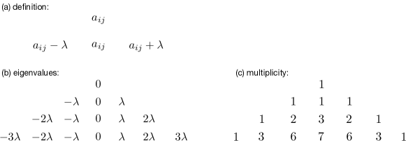
Figure 5: Eigenvalues and multiplicities of $\sum_{r=1}^{p}[G_{j}^{(r)},G_{k}^{(r)}]$.

Hence the eigenvalues of $[G_{jp},G_{kp}]=\sum_{r=1}^{p}[G_{j}^{(r)},G_{k}^{(r)}]$ are $\lambda s$ with multiplicity $\binom{p}{s}_{2}$ for $s=-p,-p+1,\cdots,p$, here $\binom{p}{s}_{2}=\sum_{i=0}^{p}(-1)^{i}\binom{p}{i}\binom{2p-2i}{p-s-i}$ is the trinomial coefficient.

Denote $\mathcal{N}_{p}=\sum_{s=0}^{p}s\binom{p}{s}_{2}$, we then have

$$(C_{p})_{jk}=\frac{1}{3^{p-1}}\|[G_{jp},G_{kp}]\|_{1}=(C_{1})_{jk}\frac{\mathcal{N}_{p}}{3^{p-1}}.$$ (262)

The Frobenius norm of $C_{p}$ is then given by

$$\|C_{p}\|_{F} =\sqrt{\sum_{jk}(C_{p})_{jk}^{2}}=\sqrt{\sum_{jk}\left((C_{1})_{jk}\frac{1}{3^{p-1}}\mathcal{N}_{p}\right)^{2}}$$ (263)

$$=\frac{1}{3^{p-1}}\mathcal{N}_{p}\sqrt{\sum_{jk}\left((C_{1})_{jk}\right)^{2}}=\frac{1}{3^{p-1}}\mathcal{N}_{p}\|C_{1}\|_{F}.$$

Using the tradeoff relations for $p$-local measurements, we have

$$\frac{1}{\nu}Tr[F_{Q}^{-1}Cov(\hat{x})^{-1}] \leq n-\frac{1}{4(n-1)}\|\frac{C_{p}}{p}\|_{F}^{2}$$ (264)

$$=n-\frac{1}{4(n-1)}\|C_{1}\|_{F}^{2}\left(\frac{1}{p3^{p-1}}\mathcal{N}_{p}\right)^{2}$$

$$=8-\frac{6}{7}\left(\frac{1}{p3^{p-1}}\mathcal{N}_{p}\right)^{2}$$

Specifically, for 2-local measurements,

$$\frac{1}{\nu}Tr[F_{Q}^{-1}Cov(\hat{x})^{-1}]\leq n-\frac{1}{4(n-1)}\|\frac{C_{2}}{2}\|_{F}^{2}=8-\frac{6}{7}\times\frac{1}{4}\times\frac{16}{9}=\frac{160}{21}\approx 7.62$$ (265)

and for 3-local measurements,

$$\frac{1}{\nu}Tr[F_{Q}^{-1}Cov(\hat{x})^{-1}]\leq n-\frac{1}{4(n-1)}\|\frac{C_{3}}{3}\|_{F}^{2}=8-\frac{6}{7}\times\frac{1}{9}\times\frac{25}{9}=\frac{1462}{189}\approx 7.74$$ (266)

If we choose the basis $\{|u\rangle_{q}\}$ as computational basis $|u\rangle_{0}=|0\rangle$, $|u\rangle_{1}=|1\rangle$, $|u\rangle_{2}=|2\rangle$, the matrices $F_{u_{q}}$ are given as

$$F_{u_{0}}=\frac{1}{2}\begin{pmatrix}1&i&0&0&0&0&0&0\\ -i&1&0&0&0&0&0&0\\ 0&0&1&0&0&0&0&\frac{\sqrt{3}}{3}\\ 0&0&0&1&i&0&0&0\\ 0&0&0&-i&1&0&0&0\\ 0&0&0&0&0&0&0&0\\ 0&0&0&0&0&0&0&0\\ 0&0&\frac{\sqrt{3}}{3}&0&0&0&0&\frac{1}{3}\end{pmatrix},F_{u_{1}}=\frac{1}{2}\begin{pmatrix}1&-i&0&0&0&0&0&0\\ i&1&0&0&0&0&0&0\\ 0&0&1&0&0&0&0&-\frac{\sqrt{3}}{3}\\ 0&0&0&0&0&0&0&0\\ 0&0&0&0&0&0&0&0\\ 0&0&0&0&0&1&i&0\\ 0&0&0&0&0&-i&1&0\\ 0&0&-\frac{\sqrt{3}}{3}&0&0&0&0&\frac{1}{3}\end{pmatrix}$$ (267)

$$F_{u_{2}}=\frac{1}{2}\begin{pmatrix}0&0&0&0&0&0&0&0\\ 0&0&0&0&0&0&0&0\\ 0&0&0&0&0&0&0&0\\ 0&0&0&1&-i&0&0&0\\ 0&0&0&i&1&0&0&0\\ 0&0&0&0&0&1&-i&0\\ 0&0&0&0&0&i&1&0\\ 0&0&0&0&0&0&0&\frac{4}{3}\end{pmatrix},\bar{F}_{Im}=\begin{pmatrix}0&1&0&0&0&0&0&0\\ -1&0&0&0&0&0&0&0\\ 0&0&0&0&0&0&0&0\\ 0&0&0&0&1&0&0&0\\ 0&0&0&-1&0&0&0&0\\ 0&0&0&0&0&0&0&0\\ 0&0&0&0&0&0&0&0\\ 0&0&0&0&0&0&0&0\end{pmatrix}$$ (268)

Let $\bar{F}=F_{u_{0}}+F_{u_{1}}^{T}+F_{u_{2}}^{T}$, this gives a bound as

$$\frac{1}{\nu}Tr[F_{Q}^{-1}Cov(\hat{x})^{-1}]\leq n-\frac{(n-2)}{(n-1)^{2}}\|\bar{F}_{Im}\|_{F}^{2}=8-\frac{6}{49}\times 4\approx 7.51,$$ (269)

If we only estimate $\{x_{1},x_{2},x_{4},x_{5}\}$, the associated matrices are given by the $4\times 4$ submatrices of the original ones,

$$C_{1}=\begin{pmatrix}0&1&\frac{1}{2}&\frac{1}{2}\\ 1&0&\frac{1}{2}&\frac{1}{2}\\ \frac{1}{2}&\frac{1}{2}&0&1\\ \frac{1}{2}&\frac{1}{2}&1&0\end{pmatrix},\bar{F}_{Im}=\begin{pmatrix}0&1&0&0\\ -1&0&0&0\\ 0&0&0&1\\ 0&0&-1&0\end{pmatrix},$$ (270)

which further gives $\|C_{1}\|_{F}=\sqrt{6}$, $\|\bar{F}_{Im}\|_{F}=2$. Then we have

$$\frac{1}{\nu}Tr[F_{Q}^{-1}Cov(\hat{x})^{-1}]\leq n-\frac{1}{4(n-1)}\|C_{1}\|_{F}^{2}=4-\frac{1}{2}=\frac{7}{2}=3.5,$$ (271)

$$\frac{1}{\nu}Tr[F_{Q}^{-1}Cov(\hat{x})^{-1}]\leq n-\frac{(n-2)}{(n-1)^{2}}\|\bar{F}_{Im}\|_{F}^{2}=4-\frac{8}{9}=\frac{28}{9}\approx 3.11.$$ (272)

For $p$-local measurements, by following the same derivation as the previous case, we have

$$\frac{1}{\nu}Tr[F_{Q}^{-1}Cov(\hat{x})^{-1}] \leq n-\frac{1}{4(n-1)}\|\frac{C_{p}}{p}\|_{F}^{2}$$ (273)

$$=n-\frac{1}{4(n-1)}\|C_{1}\|_{F}^{2}\left(\frac{1}{p3^{p-1}}\mathcal{N}_{p}\right)^{2}$$

$$=4-\frac{1}{2}\left(\frac{1}{p3^{p-1}}\mathcal{N}_{p}\right)^{2}$$

Specifically, for p=2 we have

$$\frac{1}{\nu}Tr[F_{Q}^{-1}Cov(\hat{x})^{-1}]\leq n-\frac{1}{4(n-1)}\|\frac{C_{2}}{2}\|_{F}^{2}=4-\frac{1}{2}\times\frac{1}{4}\times\frac{16}{9}=\frac{34}{9}\approx 3.78,$$ (274)

and for p=3,

$$\frac{1}{\nu}Tr[F_{Q}^{-1}Cov(\hat{x})^{-1}]\leq n-\frac{1}{4(n-1)}\|\frac{C_{3}}{3}\|_{F}^{2}=4-\frac{1}{2}\times\frac{1}{9}\times\frac{25}{9}=\frac{623}{162}\approx 3.85.$$ (275)

If we choose the basis $\{|u_{q}\rangle\}$ as the computational basis $|u_{0}\rangle=|00\rangle$, $|u_{1}\rangle=|01\rangle$, $|u_{2}\rangle=|02\rangle$, $|u_{3}\rangle=|10\rangle$,…, $|u_{8}\rangle=|22\rangle$, the imaginary part of the matrices $F_{u_{q}}$ are given as

$$F_{u_{0}Im}=\begin{pmatrix}0&\frac{1}{3}&0&0\\ -\frac{1}{3}&0&0&0\\ 0&0&0&\frac{1}{3}\\ 0&0&-\frac{1}{3}&0\end{pmatrix},F_{u_{4}Im}=\begin{pmatrix}0&-\frac{1}{3}&0&0\\ \frac{1}{3}&0&0&0\\ 0&0&0&0\\ 0&0&0&0\end{pmatrix},F_{u_{8}Im}=\begin{pmatrix}0&0&0&0\\ 0&0&0&0\\ 0&0&0&-\frac{1}{3}\\ 0&0&\frac{1}{3}&0\end{pmatrix},$$ (276)

$$F_{u_{1}Im}=F_{u_{3}Im}=\frac{1}{2}\begin{pmatrix}0&0&0&0\\ 0&0&0&0\\ 0&0&0&\frac{1}{3}\\ 0&0&-\frac{1}{3}&0\end{pmatrix},F_{u_{2}Im}=F_{u_{6}Im}=\frac{1}{2}\begin{pmatrix}0&\frac{1}{3}&0&0\\ -\frac{1}{3}&0&0&0\\ 0&0&0&0\\ 0&0&0&0\end{pmatrix},$$

$$F_{u_{5}Im}=F_{u_{7}Im}=\frac{1}{2}\begin{pmatrix}0&-\frac{1}{3}&0&0\\ \frac{1}{3}&0&0&0\\ 0&0&0&-\frac{1}{3}\\ 0&0&\frac{1}{3}&0\end{pmatrix}.$$

The optimal $\bar{F}_{Im2}$ is then given by $\bar{F}_{Im2}=F_{u_{0}Im}+F_{u_{4}Im}^{T}+F_{u_{8}Im}^{T}+(F_{u_{1}Im}+F_{u_{3}Im})+(F_{u_{2}Im}+F_{u_{6}Im})+(F_{u_{5}Im}+F_{u_{7}Im})^{T}$, i.e.,

$$\bar{F}_{Im2}=\begin{pmatrix}0&\frac{4}{3}&0&0\\ -\frac{4}{3}&0&0&0\\ 0&0&0&\frac{4}{3}\\ 0&0&-\frac{4}{3}&0\end{pmatrix},$$ (277)

which gives a tighter bound as

$$\frac{1}{\nu}Tr[F_{Q}^{-1}Cov(\hat{x})^{-1}]\leq n-\frac{(n-2)}{(n-1)^{2}}\|\frac{\bar{F}_{Im2}}{2}\|_{F}^{2}=4-\frac{2}{9}\times\frac{1}{4}\times 4\times\frac{16}{9}=4-\frac{32}{81}\approx 3.60.$$ (278)

If we only estimate $\{x_{1},x_{2},x_{5}\}$, the associated matrices are given by the $3\times 3$ submatrices of the original ones,

$$C_{1}=\begin{pmatrix}0&1&\frac{1}{2}\\ 1&0&\frac{1}{2}\\ \frac{1}{2}&\frac{1}{2}&0\end{pmatrix},\bar{F}_{Im}=\begin{pmatrix}0&1&0\\ -1&0&0\\ 0&0&0\end{pmatrix},$$ (279)

which further gives $\|C_{1}\|_{F}=\sqrt{3}$, $\|\bar{F}_{Im}\|_{F}=\sqrt{2}$. Then we have the tradeoff relations

$$\frac{1}{\nu}Tr[F_{Q}^{-1}Cov(\hat{x})^{-1}]\leq n-\frac{1}{4(n-1)}\|C_{1}\|_{F}^{2}=3-\frac{3}{8}=\frac{21}{8}=2.625,$$ (280)

$$\frac{1}{\nu}Tr[F_{Q}^{-1}Cov(\hat{x})^{-1}]\leq n-\frac{(n-2)}{(n-1)^{2}}\|\bar{F}_{Im}\|_{F}^{2}=3-\frac{1}{2}=\frac{5}{2}=2.5.$$ (281)

For $p$-local measurements, we have

$$\frac{1}{\nu}Tr[F_{Q}^{-1}Cov(\hat{x})^{-1}] \leq n-\frac{1}{4(n-1)}\|\frac{C_{p}}{p}\|_{F}^{2}$$ (282)

$$=n-\frac{1}{4(n-1)}\|C_{1}\|_{F}^{2}\left(\frac{1}{p3^{p-1}}\mathcal{N}_{p}\right)^{2}$$

$$=3-\frac{3}{8}\left(\frac{1}{p3^{p-1}}\mathcal{N}_{p}\right)^{2}$$

Specifically, for p=2,

$$\frac{1}{\nu}Tr[F_{Q}^{-1}Cov(\hat{x})^{-1}]\leq n-\frac{1}{4(n-1)}\|\frac{C_{2}}{2}\|_{F}^{2}=3-\frac{3}{8}\times\frac{1}{4}\times\frac{16}{9}=\frac{17}{6}\approx 2.83,$$ (283)

and for p=3,

$$\frac{1}{\nu}Tr[F_{Q}^{-1}Cov(\hat{x})^{-1}]\leq n-\frac{1}{4(n-1)}\|\frac{C_{3}}{3}\|_{F}^{2}=3-\frac{3}{8}\times\frac{1}{9}\times\frac{25}{9}=\frac{623}{216}\approx 2.88.$$ (284)

For 2-local measurements, if we choose the basis $\{|u_{q}\rangle\}$ as the computational basis $|u_{0}\rangle=|00\rangle$, $|u_{1}\rangle=|01\rangle$, $|u_{2}\rangle=|02\rangle$, $|u_{3}\rangle=|10\rangle$,…, $|u_{8}\rangle=|22\rangle$, the imaginary part of the matrices $F_{u_{q}}$ are given as

$$F_{u_{0}Im}=\begin{pmatrix}0&\frac{1}{3}&0\\ -\frac{1}{3}&0&0\\ 0&0&0\end{pmatrix},F_{u_{4}Im}=\begin{pmatrix}0&-\frac{1}{3}&0\\ \frac{1}{3}&0&0\\ 0&0&0\end{pmatrix},F_{u_{1}Im}=F_{u_{3}Im}=F_{u_{8}Im}=\mathbf{0},$$ (285)

$$F_{u_{2}Im}=F_{u_{6}Im}=\frac{1}{2}\begin{pmatrix}0&\frac{1}{3}&0\\ -\frac{1}{3}&0&0\\ 0&0&0\end{pmatrix},F_{u_{5}Im}=F_{u_{7}Im}=\frac{1}{2}\begin{pmatrix}0&-\frac{1}{3}&0\\ \frac{1}{3}&0&0\\ 0&0&0\end{pmatrix}.$$

The optimal $\bar{F}_{Im2}$ is then given by $\bar{F}_{Im2}=F_{u_{0}Im}+F_{u_{4}Im}^{T}+(F_{u_{2}Im}+F_{u_{6}Im})+(F_{u_{5}Im}+F_{u_{7}Im})^{T}$, i.e.,

$$\bar{F}_{Im2}=\begin{pmatrix}0&\frac{4}{3}&0\\ -\frac{4}{3}&0&0\\ 0&0&0\end{pmatrix},$$ (286)

which gives

$$\frac{1}{\nu}Tr[F_{Q}^{-1}Cov(\hat{x})^{-1}]\leq n-\frac{(n-2)}{(n-1)^{2}}\|\frac{\bar{F}_{Im2}}{2}\|_{F}^{2}=3-\frac{1}{4}\times\frac{1}{4}\times 2\times\frac{16}{9}=3-\frac{2}{9}\approx 2.78.$$ (287)

This is tighter than the bound given by $C_{2}$.

If we only estimate $\{x_{1},x_{2}\}$, the associated matrices are given by the $2\times 2$ submatrices of the original ones,

$$C_{1}=\begin{pmatrix}0&1\\ 1&0\end{pmatrix}$$ (288)

which further gives $\|C_{1}\|_{F}=\sqrt{2}$. Then we have the tradeoff relation

$$\frac{1}{\nu}Tr[F_{Q}^{-1}Cov(\hat{x})^{-1}]\leq n-\frac{1}{4(n-1)}\|C_{1}\|_{F}^{2}=2-\frac{1}{2}=\frac{3}{2}.$$ (289)

For $p$-local measurements, we have

$$\frac{1}{\nu}Tr[F_{Q}^{-1}Cov(\hat{x})^{-1}] \leq n-\frac{1}{4(n-1)}\|\frac{C_{p}}{p}\|_{F}^{2}$$ (290)

$$=n-\frac{1}{4(n-1)}\|C_{1}\|_{F}^{2}\left(\frac{1}{p3^{p-1}}\mathcal{N}_{p}\right)^{2}$$

$$=2-\frac{1}{2}\left(\frac{1}{p3^{p-1}}\mathcal{N}_{p}\right)^{2}$$

Specifically, for p=2,

$$\frac{1}{\nu}Tr[F_{Q}^{-1}Cov(\hat{x})^{-1}]\leq n-\frac{1}{4(n-1)}\|\frac{C_{2}}{2}\|_{F}^{2}=2-\frac{1}{2}\times\frac{1}{4}\times\frac{16}{9}=\frac{16}{9}\approx 1.78,$$ (291)

and for p=3,

$$\frac{1}{\nu}Tr[F_{Q}^{-1}Cov(\hat{x})^{-1}]\leq n-\frac{1}{4(n-1)}\|\frac{C_{3}}{3}\|_{F}^{2}=2-\frac{1}{2}\times\frac{1}{9}\times\frac{25}{9}=\frac{299}{162}\approx 1.85.$$ (292)

We plot the bound with different $p$ in Fig.6. It can be seen that the Holevo bound, which equals to the QCRB since the weak commutative condition holds in this case, is only achievable when $p\rightarrow\infty$.

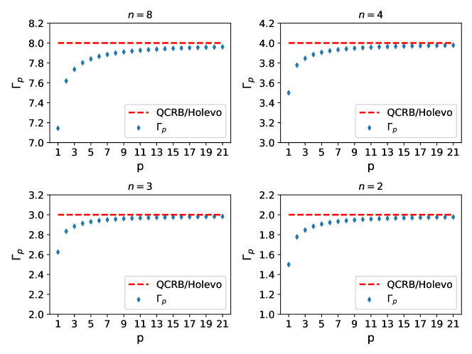
Figure 6: Upper bound on $\Gamma_{p}$ and the QCRB/Holevo bound with the number of parameters equal to $8,4,3,2$ respectively.

References

(1)
HongZhen Chen, Yu Chen, Haidong Yuan,
Distortion of Information Geometry under hirachical quantum measurements.
Phys. Rev. Letts.
(2)
Carl W. Helstrom.
Quantum Detection and Estimation Theory.
Academic Press, New York, 1976.
(3)
A. S. Holevo.
Probabilistic and Statistical Aspects of Quantum Theory.
North-Holland, Amsterdam, 1982.
(4)
Samuel L. Braunstein, Carlton M. Caves, and G. J. Milburn.
Generalized uncertainty relations: Theory, examples, and Lorentz
invariance.
Ann. Phys., 247(1):135–173, 1996.
(5)
Vittorio Giovannetti, Seth Lloyd, and Lorenzo Maccone.
Quantum-enhanced measurements: Beating the standard quantum limit.
Science, 306:1330, 2004.
(6)
Vittorio Giovannetti, Seth Lloyd, and Lorenzo Maccone.
Quantum metrology.
Phys. Rev. Lett., 96:010401, 2006.
(7)
B M Escher, R L de Matos Filho, and L Davidovich.
General framework for estimating the ultimate precision limit in
noisy quantum-enhanced metrology.
Nat. Phys., 7(5):406–411, may 2011.
(8)
Tomohisa Nagata, Ryo Okamoto, Jeremy L O’brien, Keiji Sasaki, and Shigeki
Takeuchi.
Beating the standard quantum limit with four-entangled photons.
Science, 316(5825):726–729, 2007.
(9)
B. L. Higgins, D. W. Berry, S. D. Bartlett, H. M. Wiseman, and G. J. Pryde.
Entanglement-free Heisenberg-limited phase estimation.
Nature, 450(7168):393–396, 2007.
(10)
G. Y. Xiang, B. L. Higgins, D. W. Berry, H. M. Wiseman, and G. J. Pryde.
Entanglement-enhanced measurement of a completely unknown optical
phase.
Nat. Photonics, 5:43, 2011.
(11)
Sergei Slussarenko, Morgan M Weston, Helen M Chrzanowski, Lynden K Shalm,
Varun B Verma, Sae Woo Nam, and Geoff J Pryde.
Unconditional violation of the shot-noise limit in photonic quantum
metrology.
Nature Photonics, 11(11):700, 2017.
(12)
Shakib Daryanoosh, Sergei Slussarenko, Dominic W Berry, Howard M Wiseman, and
Geoff J Pryde.
Experimental optical phase measurement approaching the exact
heisenberg limit.
Nature communications, 9(1):4606, 2018.
(13)
Haidong Yuan and Chi-Hang Fred Fung.
Quantum parameter estimation with general dynamics.
NPJ Quantum Information, 3(1):14, 2017.
(14)
Haidong Yuan and Chi-Hang Fred Fung.
Quantum metrology matrix.
Phys. Rev. A, 96 (1), 012310, 2017.
(15)
Jing Liu, Mao Zhang, Hongzhen Chen, Lingna Wang, and Haidong Yuan.
Optimal scheme for quantum metrology.
Adv. Quantum Technol, 5:2100080, 2022.
(16)
K Matsumoto.
A new approach to the cramér-rao-type bound of the pure-state
model.
Journal of Physics A: Mathematical and General,
35(13):3111–3123, mar 2002.
(17)
Peter C. Humphreys, Marco Barbieri, Animesh Datta, and Ian A. Walmsley.
Quantum enhanced multiple phase estimation.
Phys. Rev. Lett., 111:070403, Aug 2013.
(18)
Luca Pezzè, Mario A. Ciampini, Nicolò Spagnolo, Peter C. Humphreys, Animesh
Datta, Ian A. Walmsley, Marco Barbieri, Fabio Sciarrino, and Augusto Smerzi.
Optimal measurements for simultaneous quantum estimation of multiple
phases.
Phys. Rev. Lett., 119:130504, Sep 2017.
(19)
M. Hayashi, editor.
Asymptotic Theory of Quantum Statistical Inference.
World Scientific, Singapore, 2005.
(20)
Zhibo Hou, Zhao Zhang, Guo-Yong Xiang, Chuan-Feng Li, Guang-Can Guo, Hongzhen
Chen, Liqiang Liu, and Haidong Yuan.
Minimal tradeoff and ultimate precision limit of multiparameter
quantum magnetometry under the parallel scheme.
Phys. Rev. Lett., 125:020501, Jul 2020.
(21)
Federico Belliardo and Vittorio Giovannetti.
Incompatibility in quantum parameter estimation.
New Journal of Physics, 23(6):063055, jun 2021.
(23)
Zhibo Hou, Yan Jin, Hongzhen Chen, Jun-Feng Tang, Chang-Jiang Huang, Haidong
Yuan, Guo-Yong Xiang, Chuan-Feng Li, and Guang-Can Guo.
”super-heisenberg” and heisenberg scalings achieved simultaneously in
the estimation of a rotating field.
Phys. Rev. Lett., 126:070503, Feb 2021.
(24)
Jing Yang, Shengshi Pang, Yiyu Zhou, and Andrew N. Jordan.
Optimal measurements for quantum multiparameter estimation with
general states.
Phys. Rev. A, 100:032104, Sep 2019.
(25)
Nan Li, Christopher Ferrie, Jonathan A. Gross, Amir Kalev, and Carlton M.
Caves.
Fisher-symmetric informationally complete measurements for pure
states.
Phys. Rev. Lett., 116:180402, May 2016.
(26)
Huangjun Zhu and Masahito Hayashi.
Universally fisher-symmetric informationally complete measurements.
Phys. Rev. Lett., 120:030404, Jan 2018.
(27)
Magdalena Szczykulska, Tillmann Baumgratz, and Animesh Datta.
Multi-parameter quantum metrology.
Advances in Physics: X, 1(4):621–639, 2016.
(28)
Francesco Albarelli, Jamie F. Friel, and Animesh Datta.
Evaluating the holevo cramér-rao bound for multiparameter quantum
metrology.
Phys. Rev. Lett., 123:200503, Nov 2019.
(29)
Richard D. Gill and Serge Massar.
State estimation for large ensembles.
Phys. Rev. A, 61:042312, Mar 2000.
(30)
F. Albarelli, M. Barbieri, M.G. Genoni, and I. Gianani.
A perspective on multiparameter quantum metrology: From theoretical
tools to applications in quantum imaging.
Physics Letters A, 384(12):126311, 2020.
(31)
Angelo Carollo, Bernardo Spagnolo, Alexander A Dubkov, and Davide Valenti.
On quantumness in multi-parameter quantum estimation.
Journal of Statistical Mechanics: Theory and Experiment,
2019(9):094010, sep 2019.
(32)
Xiao-Ming Lu and Xiaoguang Wang.
Incorporating heisenberg’s uncertainty principle into quantum
multiparameter estimation.
Phys. Rev. Lett., 126:120503, Mar 2021.
(33)
Sammy Ragy, Marcin Jarzyna, and Rafal Demkowicz-Dobrzański.
Compatibility in multiparameter quantum metrology.
Phys. Rev. A, 94:052108, Nov 2016.
(34)
Yu Chen and Haidong Yuan.
Maximal quantum fisher information matrix.
New Journal of Physics, 19(6):063023, jun 2017.
(35)
Jing Liu, Haidong Yuan, Xiao-Ming Lu, and Xiaoguang Wang.
Quantum fisher information matrix and multiparameter estimation.
Journal of Physics A: Mathematical and Theoretical,
53(2):023001, dec 2020.
(36)
Hongzhen Chen and Haidong Yuan.
Optimal joint estimation of multiple rabi frequencies.
Phys. Rev. A, 99:032122, Mar 2019.
(37)
Francesco Albarelli, Marco Barbieri, Marco G. Genoni, and Ilaria Gianani.
A perspective on multiparameter quantum metrology: From theoretical
tools to applications in quantum imaging.
Phys. Lett. A, 384:126311, 2020.
(38)
R. Demkowicz-Dobrzański, W. Górecki, and M. Guţă.
Multi-parameter estimation beyond quantum fisher information.
J. Phys. A: Math. Theor., 53:363001, 2020.
(39)
Jasminder S. Sidhu and Pieter Kok.
Geometric perspective on quantum parameter estimation.
AVS Quantum Sci., 2:014701, 2020.
(40)
M. D. Vidrighin, G. Donati, M. G. Genoni, X.-M. Jin, W. S. Kolthammer, M. S.
Kim, A. Datta, M. Barbieri, and I. A. Walmsley.
Joint estimation of phase and phase diffusion for quantum metrology.
Nat. Commun., 5:3532, 2014.
(41)
Philip J. D. Crowley, Animesh Datta, Marco Barbieri, and I. A. Walmsley.
Tradeoff in simultaneous quantum-limited phase and loss estimation in
interferometry.
Phys. Rev. A, 89:023845, Feb 2014.
(42)
J.-D. Yue, Y.-R. Zhang, and H Fan.
Quantum-enhanced metrology for multiple phase estimation with noise.
Sci. Rep., 4:5933, 2014.
(43)
Yu-Ran Zhang and Heng Fan.
Quantum metrological bounds for vector parameters.
Phys. Rev. A, 90:043818, Oct 2014.
(44)
Jing Liu and Haidong Yuan.
Control-enhanced multiparameter quantum estimation.
Phys. Rev. A, 96:042114, Oct 2017.
(45)
Emanuele Roccia, Ilaria Gianani, Luca Mancino, Marco Sbroscia, Fabrizia Somma,
Marco G Genoni, and Marco Barbieri.
Entangling measurements for multiparameter estimation with two
qubits.
Quantum Science and Technology, 3(1):01LT01, nov 2017.
(46)
Sholeh Razavian, Matteo G. A. Paris, and Marco G. Genoni.
On the quantumness of multiparameter estimation problems for qubit
systems.
Entropy, 22(11), 2020.
(47)
Alessandro Candeloro, Matteo G.A. Paris, and Marco G. Genoni.
On the properties of the asymptotic incompatibility measure in
multiparameter quantum estimation.
arxiv, page 2107.13426, 2021.
(48)
Koichi Yamagata, Akio Fujiwara, and Richard D. Gill.
Quantum local asymptotic normality based on a new quantum likelihood
ratio.
The Annals of Statistics, 41(4):2197 – 2217, 2013.
(49)
Jonas Kahn and Mădălin Guţă.
Local asymptotic normality for finite dimensional quantum systems.
Communications in Mathematical Physics, 289:597–652, Jul 2009.
(50)
Yuxiang. Yang, Giulio Chiribella, and Masahito Hayashi.
Attaining the ultimate precision limit in quantum state estimation.
Communications in Mathematical Physics, 368:223–293, 2019.
(51)
Jun Suzuki.
Explicit formula for the holevo bound for two-parameter qubit-state
estimation problem.
Journal of Mathematical Physics, 57(4):042201, 2016.
(52)
Jasminder S. Sidhu, Yingkai Ouyang, Earl T. Campbell, and Pieter Kok.
Tight bounds on the simultaneous estimation of incompatible
parameters.
Phys. Rev. X, 11:011028, Feb 2021.
(53)
H. Nagaoka.
A new approach to cramer–rao bounds for quantum state estimation.
In Masahito Hayashi, editor, Asymptotic theory of quantum
statistical inference: Selected Papers, Singapore, 2005. World scientific.
Originally published as IEICE Technical Report, 89, 228, IT 89–42,
9–14 (1989).
(54)
H. Nagaoka.
A generalization of the simultaneous diagonalization of hermitian
matrices and its relation to quantum estimation theory.
In Masahito Hayashi, editor, Asymptotic theory of quantum
statistical inference: Selected Papers, Singapore, 2005. World scientific.
(55)
Lorcán O. Conlon, Jun. Suzuki, Ping Koy Lam, and Syed M. Assad.
Efficient computation of the nagaoka–hayashi bound for
multiparameter estimation with separable measurements.
npj Quantum Information, 7:110, Jul 2021.
(56)
Harald Cramér.
Mathematical Methods of Statistics.
Princeton University Press, Princeton, NJ, 1946.
(57)
R. A. Fisher.
On the mathematical foundations of theoretical statistics.
Philos. Trans. R. Soc. Lond. A, 222:309–368, 1922.
(58)
H. P. Robertson.
An indeterminacy relation for several observables and its classical
interpretation.
Phys. Rev., 46:794–801, Nov 1934.
(59)
D. A. Trifonov.
Generalizations of heisenberg uncertainty relation.
The European Physical Journal B - Condensed Matter and Complex
Systems, 29(2):349–353, 2002.
(60)
Masahito Hayashi and Keiji Matsumoto.
Statistical model with measurement degree of freedom and quantum
physics.
In Masahito Hayashi, editor, Asymptotic theory of quantum
statistical inference: Selected Papers, Singapore, 2005. World scientific.
Original Japanese version was published in Surikaiseki Kenkyusho
Kokyuroku, 1055:96-110, 1998.
(61)
S. Boyd and L. Vandenberghe.
Convex Optimization.
Cambridge University Press, Cambridge, 2004.
(62)
Horace Yuen and M. Lax.
Multiple parameter quantum estimation and measurement of
nonselfadjoint observables.
IRE Professional Group on Information Theory, 19:740–750,
1973.