Inexact Bregman Proximal Gradient Method and its Inertial Variant with Absolute and Relative Stopping Criteria

Abstract

The Bregman proximal gradient method (BPGM), which uses the Bregman distance as a proximity measure in the iterative scheme, has recently been re-developed for minimizing convex composite problems without the global Lipschitz gradient continuity assumption. This makes the BPGM appealing for a wide range of applications, and hence it has received growing attention in recent years. However, most existing convergence results are only obtained under the assumption that the involved subproblems are solved exactly, which is not realistic in many applications. For the BPGM to be implementable and practical, in this paper, we develop inexact versions of the BPGM by employing either an absolute-type stopping criterion or a relative-type stopping criterion solving the subproblems. The iteration complexity of $\mathcal{O}(1/k)$ and the convergence of the sequence are also established for our iBPGM under some conditions. Moreover, we develop an inertial variant of our iBPGM (denoted by v-iBPGM) and establish the iteration complexity of $\mathcal{O}(1/k^{\gamma})$, where $\gamma\geq 1$ is a restricted relative smoothness exponent. When the smooth part in the objective has a Lipschitz continuous gradient and the kernel function is strongly convex, we have $\gamma=2$ and thus the v-iBPGM improves the iteration complexity of the iBPGM from $\mathcal{O}(1/k)$ to $\mathcal{O}(1/k^{2})$, in accordance with the existing results on the exact accelerated BPGM. Finally, some preliminary numerical experiments for solving the discrete quadratic regularized optimal transport problem are conducted to illustrate the convergence behaviors of our iBPGM and v-iBPGM under different inexactness settings.

Keywords:  Proximal gradient method; Bregman distance; relative smoothness; inexact stopping criteria; Nesterov’s acceleration.

1 Introduction

In this paper, we consider the following convex composite problem:

$$\min\limits_{\bm{x}\in\mathcal{Q}}~{}F(\bm{x}):=P(\bm{x})+f(\bm{x}),$$ (1.1)

where $\mathcal{Q}\subseteq\mathbb{E}$ is a closed convex set with nonempty interior denoted by $\mathrm{int}\,\mathcal{Q}$, and $\mathbb{E}$ is a real finite dimensional Euclidean space equipped with an inner product $\langle\cdot,\cdot\rangle$ and its induced norm $\|\cdot\|$. The functions $f,\,P:\mathbb{E}\rightarrow(-\infty,\infty]$ are proper closed convex functions and $f$ is differentiable on $\mathrm{int}\,\mathcal{Q}$. Problem (1.1) is a generic optimization problem that arises in many application areas such as machine learning, data science, image/signal processing, to mention just a few, and has been extensively studied in the literature; see, for example, [5, 10, 16, 24, 27, 38, 43, 45, 47].

A classical method for solving problem (1.1) is the proximal gradient method (PGM) [22, 30] (also known as the forward-backward splitting method), whose basic iterative step is given by

$$\bm{x}^{k+1}=\mathop{\mathrm{argmin}}\limits_{\bm{x}\in\mathcal{Q}}\left\{P(\bm{x})+\langle\nabla f(\bm{x}^{k}),\,\bm{x}-\bm{x}^{k}\rangle+\frac{L}{2}\|\bm{x}-\bm{x}^{k}\|^{2}\right\},$$

where $L>0$ is a constant. This scheme is developed based on the construction of a quadratic upper approximation of the smooth part $f$. Therefore, a central assumption required in the development and analysis of the PGM is that $\nabla f$ is Lipschitz continuous on $Q$. Moreover, one can consider the Bregman distance $\mathcal{D}_{\phi}$ associated with a kernel function $\phi$ as a proximity measure (see next section for definition), and naturally generalize the PGM to the Bregman proximal gradient method (BPGM) (see, for example, [3, 5, 32, 46, 47]), whose basic iterative step reads as follows:

$$\bm{x}^{k+1}=\mathop{\mathrm{argmin}}\limits_{\bm{x}\in\mathcal{Q}}\left\{P(\bm{x})+\langle\nabla f(\bm{x}^{k}),\,\bm{x}-\bm{x}^{k}\rangle+L\mathcal{D}_{\phi}(\bm{x},\,\bm{x}^{k})\right\}.$$ (1.2)

Comparing to the PGM, the BPGM with a suitable choice of $\mathcal{D}_{\phi}$ is better able to exploit the underlying geometry/structure of the problem and possibly obtains a more tractable subproblem (1.2) (see, for example, [9, Section 5], [37, Lemma 4]). More importantly, as investigated in recent insightful works [5, 32], the BPGM can be developed based on the notion of relative smoothness, which is weaker than the longstanding global Lipschitz gradient continuity assumption. This makes the BPGM applicable for a wider range of problems, such as the Poisson inverse problem [5] and D-optimal design [32], where $f$ involves the logarithm function in the form of relative entropy and log-determinant, respectively. Because of such an appealing potential, the BPGM and its variants have gained increasing attention in recent years; see, for example, [4, 5, 12, 20, 23, 32, 45, 48, 51].

Unfortunately, although the underlying geometry/structure can possibly be captured by the kernel function, the subproblem (1.2) still has no closed-form solution in many applications and its computation may still be demanding numerically; see examples in [17, 26, 42] and the one in our numerical section. Thus, for the BPGM to be implementable and practical, it must allow one to solve the subproblem approximately with progressive accuracy and the corresponding stopping criterion should be practically verifiable. However, unlike the inexact PGM which has been widely studied under different inexact criteria (see, for example, [19, 43, 49]), the study on the inexact BPGM is still at an early stage. Kabbadj [28] recently developed an inexact BPGM by allowing an $\varepsilon$-minimizer for each subproblem (1.2). Since the optimal objective value of subproblem (1.2) is generally unknown, such an inexact stopping criterion can be difficult, if not impossible, to verify in practice. In [44], Stonyakin et al. proposed a general inexact algorithmic framework for first-order methods containing the BPGM as a special case, where an approximate solution of the subproblem (1.2) is accepted when a certain inexact condition [44, Definition 2.12] holds. In our context, their inexact condition can be covered by our absolute-type stopping criterion (AbSC) with the additional requirements that $\delta_{k}\equiv 0$ and $\bm{x}^{k+1}\equiv\widetilde{\bm{x}}^{k+1}$ (see Step 1 in Algorithm 1). But we note that their condition might be difficult to verify in some practical cases; see an example in Remark 3.1.

Over the last few decades, Nesterov’s series of seminal works [34, 35, 37] (see also [36]) on accelerated gradient methods have inspired numerous accelerated variants of the PGM (see, e.g., [10, 13, 38, 46, 47]) as well as their inexact counterparts (see, e.g., [2, 14, 27, 43, 49]). Naturally, those developments also motivated many researchers to explore whether and how the BPGM can be accelerated. A successful attempt was made by Auslender and Teboulle [3, Section 5], who proposed an improved interior gradient algorithm (a Bregman gradient scheme) for solving a special case of problem (1.1) with $P\equiv 0$ and showed that this algorithm can achieve a faster rate of $\mathcal{O}(1/k^{2})$. Later on, it was extended by Tseng [46, 47] to handle problem (1.1) in a more general composite setting. Other accelerated variants of the BPGM can also be found in [29, 46, 47]. Note that all these works [3, 29, 46, 47] just mentioned require the assumptions that $f$ has a globally Lipschitz gradient and that the kernel function of the Bregman distance is strongly convex. Until recently, based on the relative smoothness assumption and a so-called triangle scaling property of the Bregman distance, Hanzely, Richtárik and Xiao [24] developed an accelerated BPGM that attains a rate of $\mathcal{O}(1/k^{\gamma})$, where $\gamma\in(0,2]$ is the triangle scaling exponent. Later, a similar result was also derived under a slightly broader smoothness condition by Gutman and Peña [23, Section 3.3]. Very recently, Dragomir et al. [20] further showed that the rate of $\mathcal{O}(1/k)$ is indeed optimal for the BPGM to solve the class of problems merely satisfying the relative smoothness assumption, and thus the BPGM cannot be accelerated if no other regularity condition is imposed. But empirically improving the BPGM via an inertial step and a certain adaptive backtracking strategy is still possible, as discussed in [24, 33].

However, among the aforementioned works that have investigated the possibility of improving the BPGM, none of them take into account of the possible errors incurred when one solves the involved subproblem approximately. Indeed, as far as we know, the rigorous study on the inexact inertial BPGM is very limited. Stonyakin et al. [44] have developed an inexact inertial variant of the BPGM in their work. But as we have mentioned in the last paragraph, the inexact stopping criterion used in [44] can be covered by our absolute-type stopping criterion and may still require improvements regarding its practical verification. Moreover, we also note that Hien et al. [25] recently proposed a block alternating Bregman majorization-minimization framework with extrapolation, which gives an inertial BPGM if only one block of variables is considered, and employed a surrogate function for $P$ to obtain a more tractable auxiliary subproblem which possibly admits a closed-form solution. But such a surrogate function could be nontrivial to find when $P$ is complex, and the auxiliary subproblem needs to be solved exactly. Thus, the kind of inexactness considered in [25] is very different from what we consider in this paper. Moreover, replacing $P$ by its surrogate might also potentially slow down the BPGM, especially when the surrogate is not a good approximation of $P$.

In this paper, to facilitate the practical implementations of the BPGM and its inertial variant, we attempt to develop their inexact counterparts and provide theoretical insights on how the error incurred in the inexact minimization of the subproblem would affect the convergence rate in terms of the objective function value. As we shall see later, our inexact framework is developed based on either an absolute-type stopping criterion or a relative-type stopping criterion. Both of them also have a two-point feature, which is motivated by our recent works [18, 50] on a new inexact Bregman proximal point algorithm. Thus, the resulting inexact framework is rather broad and can handle different types of errors that may occur when solving the subproblem, and it is also helpful to circumvent the underlying feasibility difficulty in evaluating the Bregman distance when the problem has a complex feasible set; see Remark 3.1 for more details.

The contributions of this paper are summarized as follows.

• We develop an inexact Bregman proximal gradient method (iBPGM) based on either an absolute-type stopping criterion or a relative-type stopping criterion, both of which are distinct from the existing ones in [28, 44] and are practically verifiable. The iteration complexity of $\mathcal{O}(1/k)$ and the convergence of the sequence are also established for our iBPGM under some proper conditions.

• We develop an inertial variant of our iBPGM (denoted by v-iBPGM) and establish the iteration complexity of $\mathcal{O}(1/k^{\gamma})$ ($\gamma\geq 1$) under an additional restricted relative smoothness assumption (see Assumption C). Our result can subsume the related results in [3, 24, 46, 47] wherein the subproblem is solved exactly, and as a byproduct, our analysis indeed provides a unified treatment of these existing results which are developed under different conditions. In particular, when the smooth part in the objective has a Lipschitz continuous gradient and the kernel function is strongly convex, we have $\gamma=2$ and thus the v-iBPGM improves the iteration complexity of the iBPGM from $\mathcal{O}(1/k)$ to $\mathcal{O}(1/k^{2})$.

• We conduct some preliminary numerical experiments to evaluate the performances of our iBPGM and v-iBPGM under different inexactness settings. The computational results empirically verify the necessity of developing inexact versions of those methods and also illustrate that different methods with different types of stopping criteria do have different inherent inexactness tolerance requirements, in accordance with our theoretical results.

The rest of this paper is organized as follows. We present notation and preliminaries in Section 2. We then describe our iBPGM for solving problem (1.1) and establish the convergence results in Section 3. A possibly faster inertial variant of our iBPGM is developed and analyzed in Section 4. Some preliminary numerical results are reported in Section 5, with some concluding remarks given in Section 6.

2 Notation and preliminaries

Assume that $f:\mathbb{E}\rightarrow(-\infty,\infty]$ is a proper closed convex function. For a given $\nu\geq 0$, the $\nu$-subdifferential of $f$ at $\bm{x}\in{\rm dom}\,f$ is defined by $\partial_{\nu}f(\bm{x}):=\{\bm{d}\in\mathbb{E}:f(\bm{y})\geq f(\bm{x})+\langle\bm{d},\,\bm{y}-\bm{x}\rangle-\nu,~{}\forall\,\bm{y}\in\mathbb{E}\}$, and when $\nu=0$, $\partial_{\nu}f$ is simply denoted by $\partial f$, which is referred to as the subdifferential of $f$. The conjugate function of $f$ is the function $f^{*}:\mathbb{E}\rightarrow(-\infty,\infty]$ defined by $f^{*}(\bm{y}):=\sup\left\{\langle\bm{y},\,\bm{x}\rangle-f(\bm{x}):\bm{x}\in\mathbb{E}\right\}$. A proper closed convex function $f$ is essentially smooth if (i) $\mathrm{int}\,\mathrm{dom}\,f$ is not empty; (ii) $f$ is differentiable on $\mathrm{int}\,\mathrm{dom}\,f$; (iii) $\|\nabla f(x_{k})\|\to\infty$ for every sequence $\{x_{k}\}$ in $\mathrm{int}\,\mathrm{dom}\,f$ converging to a boundary point of $\mathrm{int}\,\mathrm{dom}\,f$; see [41, page 251].

For a vector $\bm{x}\in\mathbb{R}^{n}$, $x_{i}$ denotes its $i$-th entry, $\mathrm{Diag}(\bm{x})$ denotes the diagonal matrix whose $i$th diagonal entry is $x_{i}$, $\|\bm{x}\|$ denotes its $\ell_{2}$ (Euclidean) norm. For a matrix $A\in\mathbb{R}^{m\times n}$, $a_{ij}$ denotes its $(i,j)$th entry, $A_{:j}$ denotes its $j$th column, $\|A\|_{F}$ denotes its Frobenius norm. For a closed convex set $\mathcal{X}\subseteq\mathbb{E}$, its indicator function $\delta_{\mathcal{X}}$ is defined by $\delta_{\mathcal{X}}(\bm{x})=0$ if $\bm{x}\in\mathcal{X}$ and $\delta_{\mathcal{X}}(\bm{x})=+\infty$ otherwise.

Given a proper closed strictly convex function $\phi:\mathbb{E}\rightarrow(-\infty,\infty]$, finite at $\bm{x}$, $\bm{y}$ and differentiable at $\bm{y}$ but not necessarily at $\bm{x}$, the Bregman distance [15] between $\bm{x}$ and $\bm{y}$ associated with the kernel function $\phi$ is defined as

$$\mathcal{D}_{\phi}(\bm{x},\,\bm{y}):=\phi(\bm{x})-\phi(\bm{y})-\langle\nabla\phi(\bm{y}),\,\bm{x}-\bm{y}\rangle.$$

It is easy to see that $D_{\phi}(\bm{x},\,\bm{y})\geq 0$ and equality holds if and only if $\bm{x}=\bm{y}$ due to the strict convexity of $\phi$. When $\mathbb{E}:=\mathbb{R}^{n}$ and $\phi(\cdot):=\|\cdot\|^{2}$, $\mathcal{D}_{\phi}(\cdot,\cdot)$ readily recovers the classical squared Euclidean distance. Based on the Bregman distance, we then define the restricted relative smoothness as follows.

Definition 2.1 (Restricted relative smoothness on $\mathcal{X}$).

Let $f,\,\phi:\mathbb{E}\to(-\infty,\infty]$ be proper closed convex functions with $\mathrm{dom}\,f\supseteq\mathrm{dom}\,\phi$ and $f,\,\phi$ be differentiable on $\mathrm{int}\,\mathrm{dom}\,\phi$. Given a closed convex set $\mathcal{X}\subseteq\mathbb{E}$ with $\mathcal{X}\cap\mathrm{int}\,\mathrm{dom}\,\phi\neq\emptyset$, we say that $f$ is $L$-smooth relative to $\phi$ restricted on $\mathcal{X}$ if there exists $L\geq 0$ such that

$$f(\bm{y})\leq f(\bm{x})+\langle\nabla f(\bm{x}),\,\bm{y}-\bm{x}\rangle+L\mathcal{D}_{\phi}(\bm{y},\,\bm{x}),\quad\forall\,\bm{x}\in\mathcal{X}\cap\mathrm{int}\,\mathrm{dom}\,\phi,~{}\bm{y}\in\mathcal{X}\cap\mathrm{dom}\,\phi.$$ (2.1)

The above restricted relative smoothness modifies the original relative smoothness (or the Lipschitz-like/convexity condition) introduced in [5, 32] by imposing a restricted set $\mathcal{X}$, and it readily reduces to the original notion when $\mathcal{X}=\mathbb{E}$. Such a restriction would help to extend the notion of the relative smoothness to more choices of $(f,\,\phi)$ with a proper $\mathcal{X}$. For example, when $\nabla f$ is $L_{f}$-Lipschitz continuous on $\mathbb{R}^{n}$ and $\phi$ is $\mu_{\phi}$-strongly convex on $\mathcal{X}\subseteq\mathbb{R}^{n}$, then it can be verified that $f$ is $\frac{L_{f}}{\mu_{\phi}}$-smooth relative to $\phi$ restricted on $\mathcal{X}$, but $f$ may not be $L$-smooth relative to $\phi$ according to the original definition in [5, 32] because $\phi$ may not be strongly convex on its domain. For example, the entropy function $\phi(x)=\sum^{n}_{i=1}x_{i}(\log x_{i}-1)$ is $\frac{1}{\alpha}$-strongly convex on $[0,\,\alpha]^{n}$ with any $\alpha>0$, but it is not strongly convex on $\mathrm{dom}\,\phi=\mathbb{R}^{n}_{+}$. Therefore, employing the notion of restricted relative smoothness in Definition 2.1 could broaden the possible applications of the BPGM and its inertial variants. More discussions on the relative smoothness can be found in [5, 32].

In order to establish the rigorous analysis under the relatively smooth setting, we make the following blanket technical assumptions.

Assumption A.

Problem (1.1) and the kernel function $\phi$ satisfy the following assumptions.

• $\phi:\mathbb{E}\to(-\infty,\infty]$ is essentially smooth and strictly convex on $\mathrm{int}\,\mathrm{dom}\,\phi$. Moreover, $\overline{\mathrm{dom}}\,\phi=\mathcal{Q}$, where $\overline{\mathrm{dom}}\,\phi$ denotes the closure of $\mathrm{dom}\,\phi$.

• $P:\mathbb{E}\to(-\infty,\infty]$ is a proper closed convex function with $\mathrm{dom}\,P\cap\mathrm{int}\,\mathcal{Q}\neq\emptyset$.

• $f:\mathbb{E}\to(-\infty,\infty]$ is a proper closed convex function with $\mathrm{dom}\,f\supseteq\mathrm{dom}\,\phi$ and $f$ is differentiable on $\mathrm{int}\,\mathrm{dom}\,\phi$. Moreover, there exists a closed convex set $\mathcal{X}\supseteq\mathrm{dom}\,P\cap\mathrm{dom}\,\phi$ such that $f$ is $L$-smooth relative to $\phi$ restricted on $\mathcal{X}$.

• $F^{*}:=\inf\left\{F(\bm{x}):\bm{x}\in\mathcal{Q}\right\}>-\infty$, i.e., problem (1.1) is bounded from below.

• Each subproblem in the iBPGM and its inertial variant is well-defined in the sense that the subproblem has a unique minimizer, which lies in $\mathrm{int}\,\mathrm{dom}\,\phi$.

Note that, in Assumption A1, $\overline{\mathrm{dom}}\,\phi=\mathcal{Q}$ implies $\mathrm{int}\,\mathrm{dom}\,\phi=\mathrm{int}\,\mathcal{Q}$ due to the convexity of $\mathrm{dom}\,\phi$ and [8, Proposition 3.36(iii)]. Then, one can see from Assumptions A2&3 that

$$\mathrm{dom}\,(P+f)\cap\mathrm{int}\,\mathrm{dom}\,\phi=\mathrm{dom}\,P\cap\mathrm{int}\,\mathrm{dom}\,\phi=\mathrm{dom}\,P\cap\mathrm{int}\,\mathcal{Q}\not=\emptyset.$$

This, together with $\overline{\mathrm{dom}}\,\phi=\mathcal{Q}$ and [8, Proposition 11.1(iv)] implies that

$$F^{*}=\inf\left\{F(\bm{x}):\bm{x}\in\mathcal{Q}\right\}=\inf\left\{F(\bm{x}):\bm{x}\in\mathrm{dom}\,\phi\right\}.$$ (2.2)

Assumption A5 is standard and is commonly made for ensuring the well-posedness of Bregman-type methods. It can be satisfied when, for example, $\phi$ is strongly convex. Other sufficient conditions are given in [5, Lemma 2].

Finally, we give four supporting lemmas that will be used in the subsequent analysis. The identity in first lemma is routine to verify and the proofs of last two lemmas are relegated to Appendix A.

Lemma 2.1 (Four points identity).

Suppose that a proper closed strictly convex function $\phi:\mathbb{E}\rightarrow(-\infty,\infty]$ is finite at $\bm{a},\,\bm{b},\,\bm{c},\,\bm{d}$ and differentiable at $\bm{a},\,\bm{b}$. Then,

$$\langle\nabla\phi(\bm{a})-\nabla\phi(\bm{b}),\,\bm{c}-\bm{d}\rangle=\mathcal{D}_{\phi}(\bm{c},\,\bm{b})+\mathcal{D}_{\phi}(\bm{d},\,\bm{a})-\mathcal{D}_{\phi}(\bm{c},\,\bm{a})-\mathcal{D}_{\phi}(\bm{d},\,\bm{b}).$$ (2.3)

Lemma 2.2 ([40, Section 2.2]).

Suppose that $\{\alpha_{k}\}_{k=0}^{\infty}\subseteq\mathbb{R}$ and $\{\beta_{k}\}_{k=0}^{\infty}\subseteq\mathbb{R}_{+}$ are two sequences such that $\{\alpha_{k}\}$ is bounded from below, $\sum_{k=0}^{\infty}\beta_{k}<\infty$, and $\alpha_{k+1}\leq\alpha_{k}+\beta_{k}$ holds for all $k$. Then, $\{\alpha_{k}\}$ is convergent.

Lemma 2.3.

Let $\{\alpha_{k}\}_{k=0}^{\infty}$ be a nonnegative sequence. If $\sum^{\infty}_{k=0}\alpha_{k}<\infty$, then $\frac{1}{k}\sum^{k-1}_{i=0}i\alpha_{i}\to 0$.

Lemma 2.4.

Suppose that Assumption A holds and $\mathcal{X}$ is the closed convex set in Assumption A3. Given any $\bm{y}\in\mathcal{X}\cap\mathrm{int}\,\mathrm{dom}\,\phi$ and $\lambda\geq 0$, let $(\bm{x}^{*},\,\widetilde{\bm{x}}^{*})$ be a pair of approximate solutions of

$$\min\limits_{\bm{x}}\,P(\bm{x})+\langle\nabla f(\bm{y}),\,\bm{x}-\bm{y}\rangle+\lambda\mathcal{D}_{\phi}(\bm{x},\,\bm{y})$$

such that $\bm{x}^{*}\in\mathcal{X}\cap\mathrm{int}\,\mathrm{dom}\,\phi$, $\widetilde{\bm{x}}^{*}\in\mathrm{dom}\,P\cap\mathrm{dom}\,\phi$, and

$$\Delta\in\partial_{\delta}P(\widetilde{\bm{x}}^{*})+\nabla f(\bm{y})+\lambda(\nabla\phi(\bm{x}^{*})-\nabla\phi(\bm{y})).$$ (2.4)

Then, for any $\bm{x}\in\mathrm{dom}\,P\cap\mathrm{dom}\,\phi$, we have

$$\quad F(\widetilde{\bm{x}}^{*})-F(\bm{x})$$

$$\leq\lambda\mathcal{D}_{\phi}(\bm{x},\,\bm{y})-\lambda\mathcal{D}_{\phi}(\bm{x},\,\bm{x}^{*})-(\lambda-L)\mathcal{D}_{\phi}(\widetilde{\bm{x}}^{*},\,\bm{y})+\lambda\mathcal{D}_{\phi}(\widetilde{\bm{x}}^{*},\,\bm{x}^{*})+\delta+|\langle\Delta,\,\widetilde{\bm{x}}^{*}-\bm{x}\rangle|.$$

3 An inexact Bregman proximal gradient method

In this section, we develop an inexact Bregman proximal gradient method (iBPGM) based on two types of inexact stopping criteria for solving problem (1.1) and study the convergence properties. The complete iterative framework is presented as Algorithm 1.

Algorithm 1 An inexact Bregman proximal gradient method (iBPGM) for problem (1.1)

Input: Follow Assumption A to choose a kernel function $\phi$ with $L\geq 0$ and $\mathcal{X}\supseteq\mathrm{dom}\,P\cap\mathrm{dom}\,\phi$. Choose $\bm{x}^{0}\in\mathcal{X}\cap\mathrm{int}\,\mathrm{dom}\,\phi$ and $\widetilde{\bm{x}}^{0}\in\mathrm{dom}\,P\cap\mathrm{dom}\,\phi$. For (AbSC), choose $\lambda\geq L$ and a sequence of nonnegative scalars $\{\varepsilon_{k}\}_{k=0}^{\infty}$. For (ReSC), choose $\lambda>L$ and $0\leq\sigma<1-\lambda^{-1}L$. Set $k=0$.
while a termination criterion is not met, do

• Find a pair $(\bm{x}^{k+1},\,\widetilde{\bm{x}}^{k+1})$ and an error pair $(\Delta^{k},\delta_{k})$ by approximately solving

  $$\min\limits_{\bm{x}}\,P(\bm{x})+\langle\nabla f(\bm{x}^{k}),\,\bm{x}-\bm{x}^{k}\rangle+\lambda\mathcal{D}_{\phi}(\bm{x},\,\bm{x}^{k}),$$ (3.1)

  such that $\bm{x}^{k+1}\in\,\mathcal{X}\cap\mathrm{int}\,\mathrm{dom}\,\phi$, $\widetilde{\bm{x}}^{k+1}\in\mathrm{dom}\,P\cap\mathrm{dom}\,\phi$, and

  $$\Delta^{k}\in\partial_{\delta_{k}}P(\widetilde{\bm{x}}^{k+1})+\nabla f(\bm{x}^{k})+\lambda\big{(}\nabla\phi(\bm{x}^{k+1})-\nabla\phi(\bm{x}^{k})\big{)},$$ (3.2)

  satisfying either an absolute-type stopping criterion (AbSC) or a relative-type stopping criterion (ReSC) as follows:

  $$\textbf{(AbSC)}\qquad\|\Delta^{k}\|+\lambda^{-1}\delta_{k}+\mathcal{D}_{\phi}(\widetilde{\bm{x}}^{k+1},\,\bm{x}^{k+1})\leq\varepsilon_{k},$$

  $$\textbf{(ReSC)}\qquad\|\Delta^{k}\|=0~{}~{}\mbox{and}~{}~{}\lambda^{-1}\delta_{k}+\mathcal{D}_{\phi}(\widetilde{\bm{x}}^{k+1},\,\bm{x}^{k+1})\leq\sigma\mathcal{D}_{\phi}(\widetilde{\bm{x}}^{k+1},\,\bm{x}^{k}).$$

• Set $k=k+1$ and go to Step 1.

end while
Output: $(\bm{x}^{k},\,\widetilde{\bm{x}}^{k})$

One can see from Algorithm 1 that, at each iteration, our inexact framework allows one to approximately solve the subproblem (3.1) under condition (3.2) satisfying either an absolute-type stopping criterion (AbSC) or a relative-type stopping criterion (ReSC). Since the subproblem (3.1) has an unique solution $\bm{x}^{k,*}\in\mathrm{dom}\,P\cap\mathrm{int}\,\mathrm{dom}\,\phi$ (by Assumption A5), then condition (3.2) always holds at $\bm{x}^{k+1}=\widetilde{\bm{x}}^{k+1}=\bm{x}^{k,*}$ and hence it is achievable. When setting $\varepsilon_{k}\equiv 0$ in (AbSC) or setting $\sigma=0$ in (ReSC), it means that $\bm{x}^{k+1}$ (equals to $\widetilde{\bm{x}}^{k+1}$) should be an optimal solution of the subproblem, and thus, our iBPGM readily reduces to the exact BPGM studied in [5, 32, 47, 51]. Moreover, when the conditions $\delta_{k}\equiv 0$ and $\bm{x}^{k+1}\equiv\widetilde{\bm{x}}^{k+1}$ are imposed in (AbSC), condition (3.2) with (AbSC) is equivalent to the inexact condition considered in [44, Definition 2.12] for the subproblem (3.1), and hence our iBPGM subsumes the inexact BPGM studied in [44] as a special case.

Both inexact stopping criteria (AbSC) and (ReSC) are of two-point type (meaning that two points $\bm{x}^{k+1}$ and $\widetilde{\bm{x}}^{k+1}$ are used in the criterion), and they are inspired by the inexact stopping criterion proposed in the recent works [18, 50] for developing a new practical inexact Bregman proximal point algorithm. They may look unusual at the first glance, but actually provide a rather broad inexact framework in which the approximate solutions are handled through the error term $\Delta^{k}$ appearing on the left-hand-side of the optimality condition, $\partial_{\delta_{k}}P$ (an approximation of $\partial P$), and the deviation $\mathcal{D}_{\phi}(\widetilde{\bm{x}}^{k+1},\,\bm{x}^{k+1})$. Thus, our inexact framework is amenable to different type of errors incurred when one solves the subproblem inexactly. In particular, the admissible deviation allows $\partial_{\delta_{k}}P$ and $\nabla\phi$ to be computed at two slightly different points, respectively. Such a simple strategy would help to circumvent the possible feasibility difficulty of requiring $\bm{x}^{k+1}\in\mathrm{dom}\,P\cap\mathrm{dom}\,\nabla\phi$ by the exact BPGM studied in [5, 32, 47, 51] and by the inexact BPGM studied in [44], as exemplified in Remark 3.1. We have also noticed a recent work by Kabbadj [28], who proposed an inexact BPGM by allowing an $\varepsilon$-minimizer for the subproblem (3.1). However, such an inexact condition cannot be directly used in practical implementations since the optimal objective value of the subproblem is generally unknown a priori.

One can also observe that the main difference between (AbSC) and (ReSC) is the strategy to control the error incurred in the inexact computation of the subproblem. In (AbSC), at each iteration, the error $\|\Delta^{k}\|+\lambda^{-1}\delta_{k}+\mathcal{D}_{\phi}(\widetilde{\bm{x}}^{k+1},\,\bm{x}^{k+1})$ is simply controlled by a prespecified tolerance parameter $\varepsilon_{k}$. This is a natural and common way to design an inexact stopping criterion. To guarantee the progressive accuracy and convergence under this type of criterion, certain summable conditions (see, for example, Theorem 3.1) are also required on the error-tolerance sequence $\{\varepsilon_{k}\}_{k=0}^{\infty}$, which may need careful tuning for the iBPGM to achieve good practical efficiency, as seen from Figure 1 in the numerical section. In contrast, in (ReSC), the error $\lambda^{-1}\delta_{k}+\mathcal{D}_{\phi}(\widetilde{\bm{x}}^{k+1},\,\bm{x}^{k+1})$ is controlled by the difference $\sigma\mathcal{D}_{\phi}(\widetilde{\bm{x}}^{k+1},\,\bm{x}^{k})$, where only a single tolerance parameter $\sigma$ is involved and thus the corresponding parameter tuning is typically easier. But the computation of $\mathcal{D}_{\phi}(\widetilde{\bm{x}}^{k+1},\,\bm{x}^{k})$ may also incur non-negligible extra cost, especially when the problem size is large. Moreover, in our current convergence analysis, we also require $\|\Delta^{k}\|=0$ for (ReSC). Although such a requirement can be satisfied in many cases (see examples in [18, 50] and the one in our numerical section), it may narrow the applicability of (ReSC). It is interesting to exploit whether such a requirement can be removed, which we leave for future research. The preliminary numerical study on the performances of our iBPGM under these two types of stopping criteria can be found in Section 5.

Remark 3.1 (Comments on the underlying feasibility difficulty).

To illustrate the underlying feasibility difficulty when solving the subproblem in the BPGM, we give the following example, which is also a test problem in our numerical experiments. Given $A\in\mathbb{R}^{m\times n}$ and $\bm{b}\in\mathbb{R}^{m}$, let $P$ be an indicator function $\delta_{\mathcal{C}}$ with $\mathcal{C}:=\{\bm{x}\in\mathbb{R}^{n}:A\bm{x}=\bm{b},\,\bm{x}\geq 0\}$, and consider the entropy function $\phi(\bm{x})=\sum_{i=1}^{n}x_{i}(\log x_{i}-1)$ as the kernel function with dom $\phi=\mathbb{R}^{n}_{+}$. Then, the subproblem (3.1) can be expressed as

$$\min\limits_{\bm{x}}~{}\langle\nabla f(\bm{x}^{k}),\,\bm{x}-\bm{x}^{k}\rangle+L\mathcal{D}_{\phi}(\bm{x},\,\bm{x}^{k})\quad\mathrm{s.t.}\quad A\bm{x}=\bm{b},~{}~{}\bm{x}\geq 0.$$ (3.3)

Thus, when employing the exact BPGM in [5, 32, 47, 51] or the inexact BPGM in [44], one needs to find the exact solution or an inexact solution $\bar{\bm{x}}^{k+1}$ that should be strictly contained in $\mathrm{dom}\,P\cap\mathrm{dom}\,\nabla\phi=\{\bm{x}\in\mathbb{R}^{n}:A\bm{x}=\bm{b},\,\bm{x}>0\}=:\mathrm{relin}\,\mathcal{C}$ (namely, the relative interior of $\mathcal{C}$). However, for most choices of $A$, a subroutine for solving (3.3) may only return a candidate approximate solution $\bm{x}^{k+1}$ that is located outside $\mathcal{C}$. Hence, one has to further perform a proper projection/rounding step at $\bm{x}^{k+1}$ to compute an approximate solution $\bar{\bm{x}}^{k+1}$ in $\mathrm{relin}\,\mathcal{C}$ and then check the inexact condition at $\bar{\bm{x}}^{k+1}$. Due to the non-closedness of $\mathrm{relin}\,\mathcal{C}$, this step is indeed difficult to implement especially when some entries of the exact solution are very close to zero. In contrast, our two-point inexact condition requires separately $\bm{x}^{k+1}\in\mathcal{X}\cap\mathrm{int}\,\mathrm{dom}\,\phi$ and $\widetilde{\bm{x}}^{k+1}\in\mathrm{dom}\,P\cap\mathrm{dom}\,\phi=\mathcal{C}$, where $\mathcal{X}\supseteq\mathrm{dom}\,P\cap\mathrm{dom}\,\phi$ can be any closed convex set satisfying Assumption A3. The point $\bm{x}^{k+1}$ (which is generally located outside $\mathcal{C}$) can be easily obtained from the subroutine and the point $\widetilde{\bm{x}}^{k+1}$ can be computed by performing a proper projection/rounding step at $\bm{x}^{k+1}$ over $\mathcal{C}$, which is clearly easier and more practical than computing a point in $\mathrm{relin}\,\mathcal{C}$. In this regard, our iBPGM is more favorable than the exact BPGM in [5, 32, 47, 51] and the inexact BPGM in [44]. More discussions on the potential advantages of such a two-point-type inexact condition over existing ones can be found in [50, Section 4].

We next establish the convergence of our iBPGM under the (AbSC) or (ReSC) stopping criterion when solving the subproblems. The analysis is inspired by [5, 32], but is more involved due to the approximate minimization of the subproblem under (AbSC) or (ReSC). We first give the following sufficient-descent-like property.

Lemma 3.1.

Suppose that Assumption A holds. Let $\{\bm{x}^{k}\}$ and $\{\widetilde{\bm{x}}^{k}\}$ be the sequences generated by the iBPGM in Algorithm 1. Then, for any $k\geq 0$ and any $\bm{x}\in\mathrm{dom}\,P\cap\mathrm{dom}\,\phi$,

$$F(\widetilde{\bm{x}}^{k+1})-F(\bm{x}) \leq\lambda\mathcal{D}_{\phi}(\bm{x},\,\bm{x}^{k})-\lambda\mathcal{D}_{\phi}(\bm{x},\,\bm{x}^{k+1})-(\lambda-L)\mathcal{D}_{\phi}(\widetilde{\bm{x}}^{k+1},\,\bm{x}^{k})$$ (3.4)

$$\qquad+\lambda\big{(}\mathcal{D}_{\phi}(\widetilde{\bm{x}}^{k+1},\,\bm{x}^{k+1})+\lambda^{-1}\delta_{k}\big{)}+|\langle\Delta^{k},\,\widetilde{\bm{x}}^{k+1}-\bm{x}\rangle|.$$

Proof.

The desired result can be easily obtained by applying Lemma 2.4 with $\widetilde{\bm{x}}^{*}=\widetilde{\bm{x}}^{k+1}$, $\bm{x}^{*}=\bm{x}^{k+1}$ and $\bm{y}=\bm{x}^{k}$.      $\Box$

We then have the following results concerning the convergence of the function value.

Theorem 3.1 (Iteration complexity of the iBPGM with (AbSC)).

Suppose that Assumption A holds and $\lambda\geq L$. Let $\{\bm{x}^{k}\}$ and $\{\widetilde{\bm{x}}^{k}\}$ be the sequences generated by the iBPGM with (AbSC) in Algorithm 1, and let $e(\bm{x}):=F(\bm{x})-F^{*}$, where $F^{*}:=\inf\left\{F(\bm{x}):\bm{x}\in\mathcal{Q}\right\}>-\infty$. The following statements hold.

• (Summability) For any $\bm{x}\in\mathrm{dom}\,P\cap\mathrm{dom}\,\phi$, we have that

  $$(\lambda-L){\textstyle\sum^{k}_{i=0}}\mathcal{D}_{\phi}(\widetilde{\bm{x}}^{i+1},\,\bm{x}^{i})\leq\lambda\mathcal{D}_{\phi}(\bm{x},\,\bm{x}^{0})+ke(\bm{x})+(\|\bm{x}\|+\lambda){\textstyle\sum^{k}_{i=0}}\varepsilon_{i}+{\textstyle\sum^{k}_{i=0}}|\langle\Delta^{i},\,\widetilde{\bm{x}}^{i+1}\rangle|.$$

  Moreover, if problem (1.1) has an optimal solution $\bm{x}^{*}\in\mathrm{dom}\,\phi$, $\lambda>L$, $\sum\varepsilon_{k}<\infty$ and $\sum|\langle\Delta^{k},\,\widetilde{\bm{x}}^{k+1}\rangle|<\infty$, then $\sum^{\infty}_{k=0}\mathcal{D}_{\phi}(\widetilde{\bm{x}}^{k+1},\,\bm{x}^{k})<\infty$.

• (At the averaged iterate) For any $k\geq 0$ and any $\bm{x}\in\mathrm{dom}\,P\cap\mathrm{dom}\,\phi$, we have that

  $$\quad F\left(\frac{1}{k+1}\sum^{k}_{i=0}\widetilde{\bm{x}}^{i+1}\right)-F(\bm{x})$$ (3.5)

  $$\leq\frac{1}{k+1}\left(\lambda\mathcal{D}_{\phi}(\bm{x},\,\bm{x}^{0})+(\|\bm{x}\|+\lambda)\sum^{k}_{i=0}\varepsilon_{i}+\sum^{k}_{i=0}|\langle\Delta^{i},\,\widetilde{\bm{x}}^{i+1}\rangle|\right).$$

  Moreover, if $\frac{1}{k}\sum^{k-1}_{i=0}\varepsilon_{i}\to 0$ and $\frac{1}{k}\sum^{k-1}_{i=0}|\langle\Delta^{i},\,\widetilde{\bm{x}}^{i+1}\rangle|\to 0$, then we get $F\big{(}{\textstyle\frac{1}{k}\sum^{k-1}_{i=0}}\,\widetilde{\bm{x}}^{i+1}\big{)}\to F^{*}$. In addition, if problem (1.1) has an optimal solution $\bm{x}^{*}\in\mathrm{dom}\,\phi$, $\sum\varepsilon_{k}<\infty$ and $\sum|\langle\Delta^{k},\,\widetilde{\bm{x}}^{k+1}\rangle|<\infty$, then we have that

  $$F\left(\frac{1}{k}\sum^{k-1}_{i=0}\,\widetilde{\bm{x}}^{i+1}\right)-F^{*}\leq\mathcal{O}\left(\frac{1}{k}\right).$$

• (At the last iterate) For any $k\geq 0$ and any $\bm{x}\in\mathrm{dom}\,P\cap\mathrm{dom}\,\phi$, we have that

  $$\quad F(\widetilde{\bm{x}}^{k+1})-F(\bm{x})$$ (3.6)

  $$\leq\frac{1}{k+1}\left(\lambda\mathcal{D}_{\phi}(\bm{x},\,\bm{x}^{0})+(\|\bm{x}\|+2\lambda)\sum^{k}_{i=0}\big{(}\varepsilon_{i}+i\varepsilon_{i}\big{)}+\sum^{k}_{i=0}\big{(}|\langle\Delta^{i},\,\widetilde{\bm{x}}^{i+1}\rangle|+i|\langle\Delta^{i},\,\widetilde{\bm{x}}^{i+1}-\widetilde{\bm{x}}^{i}\rangle|\big{)}\right).$$

  Moreover, if $\frac{1}{k}\sum^{k-1}_{i=0}i\varepsilon_{i}\to 0$ and $\frac{1}{k}\sum^{k-1}_{i=0}\big{(}|\langle\Delta^{i},\,\widetilde{\bm{x}}^{i+1}\rangle|+i|\langle\Delta^{i},\,\widetilde{\bm{x}}^{i+1}-\widetilde{\bm{x}}^{i}\rangle|\big{)}\to 0$, then we get $F(\widetilde{\bm{x}}^{k})\to F^{*}$. In addition, if problem (1.1) has an optimal solution $\bm{x}^{*}\in\mathrm{dom}\,\phi$, $\sum k\varepsilon_{k}<\infty$ and $\sum\big{(}|\langle\Delta^{k},\,\widetilde{\bm{x}}^{k+1}\rangle|+k|\langle\Delta^{k},\,\widetilde{\bm{x}}^{k+1}-\widetilde{\bm{x}}^{k}\rangle|\big{)}<\infty$, the we have that

  $$F(\widetilde{\bm{x}}^{k})-F^{*}\leq\mathcal{O}\left(\frac{1}{k}\right).$$

Proof.

Statement (i). First, it follows from (3.4) and (AbSC) that, for any $i\geq 0$ and any $\bm{x}\in\mathrm{dom}\,P\cap\mathrm{dom}\,\phi$,

$$\quad F(\widetilde{\bm{x}}^{i+1})-F(\bm{x})\;\leq\;\lambda\mathcal{D}_{\phi}(\bm{x},\,\bm{x}^{i})-\lambda\mathcal{D}_{\phi}(\bm{x},\,\bm{x}^{i+1})-(\lambda-L)\mathcal{D}_{\phi}(\widetilde{\bm{x}}^{i+1},\,\bm{x}^{i})$$ (3.7)

$$\hskip 105.27519pt+|\langle\Delta^{i},\,\widetilde{\bm{x}}^{i+1}-\bm{x}\rangle|+\lambda\big{(}\mathcal{D}_{\phi}(\widetilde{\bm{x}}^{i+1},\,\bm{x}^{i+1})+\lambda^{-1}\delta_{i}\big{)}$$

$$\leq\lambda\mathcal{D}_{\phi}(\bm{x},\,\bm{x}^{i})-\lambda\mathcal{D}_{\phi}(\bm{x},\,\bm{x}^{i+1})-(\lambda-L)\mathcal{D}_{\phi}(\widetilde{\bm{x}}^{i+1},\,\bm{x}^{i})+(\|\bm{x}\|+\lambda)\varepsilon_{i}+|\langle\Delta^{i},\,\widetilde{\bm{x}}^{i+1}\rangle|,$$

which, together with $F(\widetilde{\bm{x}}^{i+1})\geq F^{*}$ for all $i\geq 0$, implies that

$$(\lambda-L)\mathcal{D}_{\phi}(\widetilde{\bm{x}}^{i+1},\,\bm{x}^{i})\leq\lambda\mathcal{D}_{\phi}(\bm{x},\,\bm{x}^{i})-\lambda\mathcal{D}_{\phi}(\bm{x},\,\bm{x}^{i+1})+e(\bm{x})+(\|\bm{x}\|+\lambda)\varepsilon_{i}+|\langle\Delta^{i},\,\widetilde{\bm{x}}^{i+1}\rangle|.$$

Summing this inequality from $i=0$ to $i=k$ yields

$$\quad(\lambda-L){\textstyle\sum^{k}_{i=0}}\mathcal{D}_{\phi}(\widetilde{\bm{x}}^{i+1},\,\bm{x}^{i})$$

$$\leq\lambda\mathcal{D}_{\phi}(\bm{x},\,\bm{x}^{0})-\lambda\mathcal{D}_{\phi}(\bm{x},\,\bm{x}^{k+1})+ke(\bm{x})+(\|\bm{x}\|+\lambda){\textstyle\sum^{k}_{i=0}}\varepsilon_{i}+{\textstyle\sum^{k}_{i=0}}|\langle\Delta^{i},\,\widetilde{\bm{x}}^{i+1}\rangle|$$

$$\leq\lambda\mathcal{D}_{\phi}(\bm{x},\,\bm{x}^{0})+ke(\bm{x})+(\|\bm{x}\|+\lambda){\textstyle\sum^{k}_{i=0}}\varepsilon_{i}+{\textstyle\sum^{k}_{i=0}}|\langle\Delta^{i},\,\widetilde{\bm{x}}^{i+1}\rangle|.$$

Moreover, if problem (1.1) has an optimal solution $\bm{x}^{*}\in\mathrm{dom}\,\phi$, we can substitute $\bm{x}^{*}$ in the above relation and obtain from $e(\bm{x}^{*})=0$ that

$$(\lambda-L){\textstyle\sum^{k}_{i=0}}\mathcal{D}_{\phi}(\widetilde{\bm{x}}^{i+1},\,\bm{x}^{i})\leq\lambda\mathcal{D}_{\phi}(\bm{x}^{*},\,\bm{x}^{0})+(\|\bm{x}^{*}\|+\lambda){\textstyle\sum^{k}_{i=0}}\varepsilon_{i}+{\textstyle\sum^{k}_{i=0}}|\langle\Delta^{i},\,\widetilde{\bm{x}}^{i+1}\rangle|.$$

Thus, if, in addition, $\lambda>L$, $\sum\varepsilon_{k}<\infty$ and $\sum|\langle\Delta^{k},\,\widetilde{\bm{x}}^{k+1}\rangle|<\infty$, one can conclude that $\sum^{\infty}_{k=0}\mathcal{D}_{\phi}(\widetilde{\bm{x}}^{k+1},\,\bm{x}^{k})<\infty$.

Statement (ii). From (3.7) and $\lambda\geq L$, we see that, for any $i\geq 0$,

$$F(\widetilde{\bm{x}}^{i+1})-F(\bm{x})\leq\lambda\mathcal{D}_{\phi}(\bm{x},\,\bm{x}^{i})-\lambda\mathcal{D}_{\phi}(\bm{x},\,\bm{x}^{i+1})+(\|\bm{x}\|+\lambda)\varepsilon_{i}+|\langle\Delta^{i},\,\widetilde{\bm{x}}^{i+1}\rangle|.$$

Summing this inequality from $i=0$ to $i=k$ gives

$$\quad{\textstyle\sum^{k}_{i=0}}F(\widetilde{\bm{x}}^{i+1})-(k+1)F(\bm{x})$$ (3.8)

$$\leq\lambda\mathcal{D}_{\phi}(\bm{x},\,\bm{x}^{0})-\lambda\mathcal{D}_{\phi}(\bm{x},\,\bm{x}^{k+1})+(\|\bm{x}\|+\lambda){\textstyle\sum^{k}_{i=0}}\varepsilon_{i}+{\textstyle\sum^{k}_{i=0}}|\langle\Delta^{i},\,\widetilde{\bm{x}}^{i+1}\rangle|.$$

Using this inequality and $F\big{(}\frac{1}{k+1}\sum^{k}_{i=0}\widetilde{\bm{x}}^{i+1}\big{)}\leq\frac{1}{k+1}\sum^{k}_{i=0}F(\widetilde{\bm{x}}^{i+1})$ (by the convexity of $F$), we obtain (3.5).

Moreover, if $\frac{1}{k}\sum^{k-1}_{i=0}\varepsilon_{i}\to 0$ and $\frac{1}{k}\sum^{k-1}_{i=0}|\langle\Delta^{i},\,\widetilde{\bm{x}}^{i+1}\rangle|\to 0$, one can see from (3.5) that

$$\limsup\limits_{k\to\infty}\,F\big{(}{\textstyle\frac{1}{k}\sum^{k-1}_{i=0}}\,\widetilde{\bm{x}}^{i+1}\big{)}\leq F(\bm{x}),\quad\forall\,\bm{x}\in\mathrm{dom}\,P\cap\mathrm{dom}\,\phi.$$

This together with $\frac{1}{k}\sum^{k-1}_{i=0}\widetilde{\bm{x}}^{i+1}\in\mathrm{dom}\,P\cap\mathrm{dom}\,\phi\subseteq\mathrm{dom}\,P\cap\mathrm{dom}\,f\cap Q$ and (2.2) implies that

$$F^{*}\leq\liminf\limits_{k\to\infty}\,F\big{(}{\textstyle\frac{1}{k}\sum^{k-1}_{i=0}}\,\widetilde{\bm{x}}^{i+1}\big{)}\leq\limsup\limits_{k\to\infty}\,F\big{(}{\textstyle\frac{1}{k}\sum^{k-1}_{i=0}}\,\widetilde{\bm{x}}^{i+1}\big{)}\leq F^{*},$$

from which, we can conclude that $F\big{(}{\textstyle\frac{1}{k}\sum^{k-1}_{i=0}}\widetilde{\bm{x}}^{i+1}\big{)}\to F^{*}$.

In addition, if problem (1.1) has an optimal solution $\bm{x}^{*}\in\mathrm{dom}\,\phi$, $\sum\varepsilon_{k}<\infty$ and $\sum|\langle\Delta^{k},\,\widetilde{\bm{x}}^{k+1}\rangle|<\infty$, one can see from (3.5) with $\bm{x}^{*}$ in place of $\bm{x}$ that $F\big{(}\frac{1}{k}\sum^{k-1}_{i=0}\widetilde{\bm{x}}^{i+1}\big{)}-F^{*}\leq\mathcal{O}(k^{-1})$.

Statement (iii). For any $i\geq 0$, by setting $\bm{x}=\widetilde{\bm{x}}^{i}$ in (3.4), we obtain

$$F(\widetilde{\bm{x}}^{i+1})-F(\widetilde{\bm{x}}^{i}) \leq\lambda\mathcal{D}_{\phi}(\widetilde{\bm{x}}^{i},\,\bm{x}^{i})-\lambda\mathcal{D}_{\phi}(\widetilde{\bm{x}}^{i},\,\bm{x}^{i+1})-(\lambda-L)\mathcal{D}_{\phi}(\widetilde{\bm{x}}^{i+1},\,\bm{x}^{i})$$

$$\qquad+\lambda\big{(}\mathcal{D}_{\phi}(\widetilde{\bm{x}}^{i+1},\,\bm{x}^{i+1})+\lambda^{-1}\delta_{i}\big{)}+|\langle\Delta^{i},\,\widetilde{\bm{x}}^{i+1}-\widetilde{\bm{x}}^{i}\rangle|$$

$$\leq\lambda(\varepsilon_{i}+\varepsilon_{i-1})+|\langle\Delta^{i},\,\widetilde{\bm{x}}^{i+1}-\widetilde{\bm{x}}^{i}\rangle|,$$

where the last inequality follows from $\lambda\geq L$ and (AbSC). Then, we see that, for any $i\geq 0$,

$$iF(\widetilde{\bm{x}}^{i+1}) \leq iF(\widetilde{\bm{x}}^{i})+\lambda i(\varepsilon_{i}+\varepsilon_{i-1})+i|\langle\Delta^{i},\,\widetilde{\bm{x}}^{i+1}-\widetilde{\bm{x}}^{i}\rangle|$$

$$~{}~{}\Longleftrightarrow~{}~{}F(\widetilde{\bm{x}}^{i+1}) \geq(i+1)F(\widetilde{\bm{x}}^{i+1})-iF(\widetilde{\bm{x}}^{i})-\lambda i(\varepsilon_{i}+\varepsilon_{i-1})-i|\langle\Delta^{i},\,\widetilde{\bm{x}}^{i+1}-\widetilde{\bm{x}}^{i}\rangle|,$$

which can induce that

$${\textstyle\sum^{k}_{i=0}}F(\widetilde{\bm{x}}^{i+1})\geq(k+1)F(\widetilde{\bm{x}}^{k+1})-\lambda{\textstyle\sum^{k}_{i=0}}\,i(\varepsilon_{i}+\varepsilon_{i-1})-{\textstyle\sum^{k}_{i=0}}\,i|\langle\Delta^{i},\,\widetilde{\bm{x}}^{i+1}-\widetilde{\bm{x}}^{i}\rangle|.$$

This together with (3.8) implies that

$$\quad(k+1)\big{(}F(\widetilde{\bm{x}}^{k+1})-F(\bm{x})\big{)}$$

$$\leq{\textstyle\sum^{k}_{i=0}}F(\widetilde{\bm{x}}^{i+1})-(k+1)F(\bm{x})+\lambda{\textstyle\sum^{k}_{i=0}}\,i(\varepsilon_{i}+\varepsilon_{i-1})+{\textstyle\sum^{k}_{i=0}}\,i|\langle\Delta^{i},\,\widetilde{\bm{x}}^{i+1}-\widetilde{\bm{x}}^{i}\rangle|$$

$$\leq\lambda\mathcal{D}_{\phi}(\bm{x},\,\bm{x}^{0})-\lambda\mathcal{D}_{\phi}(\bm{x},\,\bm{x}^{k+1})+(\|\bm{x}\|+\lambda){\textstyle\sum^{k}_{i=0}}\,\varepsilon_{i}+\lambda{\textstyle\sum^{k}_{i=0}}\,i(\varepsilon_{i}+\varepsilon_{i-1})$$

$$\qquad+{\textstyle\sum^{k}_{i=0}}|\langle\Delta^{i},\,\widetilde{\bm{x}}^{i+1}\rangle|+{\textstyle\sum^{k}_{i=0}}\,i|\langle\Delta^{i},\,\widetilde{\bm{x}}^{i+1}-\widetilde{\bm{x}}^{i}\rangle|$$

$$\leq\lambda\mathcal{D}_{\phi}(\bm{x},\,\bm{x}^{0})-\lambda\mathcal{D}_{\phi}(\bm{x},\,\bm{x}^{k+1})+(\|\bm{x}\|+2\lambda){\textstyle\sum^{k}_{i=0}}\,\big{(}\varepsilon_{i}+i\varepsilon_{i}\big{)}$$

$$\qquad+{\textstyle\sum^{k}_{i=0}}\,\big{(}|\langle\Delta^{i},\,\widetilde{\bm{x}}^{i+1}\rangle|+i|\langle\Delta^{i},\,\widetilde{\bm{x}}^{i+1}-\widetilde{\bm{x}}^{i}\rangle|\big{)}.$$

Dividing the above inequality by $k+1$, we can get (3.6).

Moreover, if $\frac{1}{k}\sum^{k-1}_{i=0}i\varepsilon_{i}\to 0$ (which readily yields $\frac{1}{k}\sum^{k-1}_{i=0}\varepsilon_{i}\to 0$) and $\frac{1}{k}\sum^{k-1}_{i=0}\big{(}|\langle\Delta^{i},\,\widetilde{\bm{x}}^{i+1}\rangle|+i|\langle\Delta^{i},\,\widetilde{\bm{x}}^{i+1}-\widetilde{\bm{x}}^{i}\rangle|\big{)}\to 0$, it is easy to see from (3.6) that

$$\limsup\limits_{k\to\infty}\,F(\widetilde{\bm{x}}^{k})\leq F(\bm{x}),\quad\forall\,\bm{x}\in\mathrm{dom}\,P\cap\mathrm{dom}\,\phi.$$

This, together with $\widetilde{\bm{x}}^{k}\in\mathrm{dom}\,P\cap\mathrm{dom}\,\phi\subseteq\mathrm{dom}\,P\cap\mathrm{dom}\,f\cap Q$ and (2.2), implies that

$$F^{*}\leq\liminf\limits_{k\to\infty}\,F(\widetilde{\bm{x}}^{k})\leq\limsup\limits_{k\to\infty}\,F(\widetilde{\bm{x}}^{k})\leq F^{*},$$

from which we can conclude that $F(\widetilde{\bm{x}}^{k})\to F^{*}$.

In addition, $\sum k\varepsilon_{k}<\infty$ yields $\sum\varepsilon_{k}<\infty$. Thus, if problem (1.1) has an optimal solution $\bm{x}^{*}\in\mathrm{dom}\,\phi$, $\sum k\varepsilon_{k}<\infty$ and $\sum\big{(}|\langle\Delta^{k},\,\widetilde{\bm{x}}^{k+1}\rangle|+k|\langle\Delta^{k},\,\widetilde{\bm{x}}^{k+1}-\widetilde{\bm{x}}^{k}\rangle|\big{)}<\infty$, we can obtain from (3.6) with $\bm{x}^{*}$ in place of $\bm{x}$ that $F(\widetilde{\bm{x}}^{k})-F^{*}\leq\mathcal{O}(k^{-1})$. This completes the proof.      $\Box$

Remark 3.2 (Comments on iteration complexity of the iBPGM with (AbSC)).

We see from Theorem 3.1 that, under proper summable-error conditions, the convergence of the function value achieves the rate of $\mathcal{O}(1/k)$ at both the averaged iterate ${\textstyle\frac{1}{k}\sum^{k-1}_{i=0}}\,\widetilde{\bm{x}}^{i+1}$ and the last iterate $\widetilde{\bm{x}}^{k}$. The latter result requires (unsurprisingly) stronger summability conditions and covers the related complexity results in [5, 32, 51] wherein each subproblem is solved exactly. Next we comment on how the condition $\sum|\langle\Delta^{k},\,\widetilde{\bm{x}}^{k+1}\rangle|<\infty$ (or $\sum\big{(}|\langle\Delta^{k},\,\widetilde{\bm{x}}^{k+1}\rangle|+k|\langle\Delta^{k},\,\widetilde{\bm{x}}^{k+1}-\widetilde{\bm{x}}^{k}\rangle|\big{)}<\infty$) can be ensured. First, as is the case in our experiments, if no error occurs on the left-hand-side of the optimality condition (3.2) (namely, $\Delta^{k}=0$) when applying a certain subroutine for solving the subproblem, such summable conditions can be readily satisfied. Moreover, if one knows a priori that $\{\widetilde{\bm{x}}^{k}\}$ will be bounded (for example, when $\mathrm{dom}\,P\cap\mathrm{dom}\,\phi$ is bounded as the test problem in our numerical experiments), then it readily reduces to $\sum\|\Delta^{k}\|<\infty$ (or $\sum k\|\Delta^{k}\|<\infty$), which can be guaranteed by $\sum\varepsilon_{k}<\infty$ (or $\sum k\varepsilon_{k}<\infty$). In addition, one could also set an arbitrarily summable nonnegative sequence $\{\eta_{k}\}$, and during the iterations, check that $|\langle\Delta^{k},\,\widetilde{\bm{x}}^{k+1}\rangle|\leq\eta_{k}$ (or $|\langle\Delta^{k},\,\widetilde{\bm{x}}^{k+1}\rangle|+k|\langle\Delta^{k},\,\widetilde{\bm{x}}^{k+1}-\widetilde{\bm{x}}^{k}\rangle|\leq\eta_{k}$). This then ensures that $\sum|\langle\Delta^{k},\,\widetilde{\bm{x}}^{k+1}\rangle|<\infty$ (or $\sum\big{(}|\langle\Delta^{k},\,\widetilde{\bm{x}}^{k+1}\rangle|+k|\langle\Delta^{k},\,\widetilde{\bm{x}}^{k+1}-\widetilde{\bm{x}}^{k}\rangle|\big{)}<\infty$). The last summability requirement also indicates that if $\{\widetilde{\bm{x}}^{k}\}$ appears to be unbounded, one may need to drive $\Delta^{k}$ to zero more quickly.

We next study the iteration complexity of the iBPGM with (ReSC).

Theorem 3.2 (Iteration complexity of the iBPGM with (ReSC)).

Suppose that Assumption A holds, $\lambda>L$, and $0<\sigma<\frac{\lambda-L}{\lambda}$. Let $\{\bm{x}^{k}\}$ and $\{\widetilde{\bm{x}}^{k}\}$ be the sequences generated by the iBPGM with the stopping condition (ReSC) in Algorithm 1, and let $e(\bm{x}):=F(\bm{x})-F^{*}$, where $F^{*}:=\inf\left\{F(\bm{x}):\bm{x}\in\mathcal{Q}\right\}>-\infty$. Then, the following statements hold.

• (Summability) For any $\bm{x}\in\mathrm{dom}\,P\cap\mathrm{dom}\,\phi$, we have that

  $${\textstyle\sum^{k}_{i=0}}\mathcal{D}_{\phi}(\widetilde{\bm{x}}^{i+1},\,\bm{x}^{i})\leq(\lambda-L-\lambda\sigma)^{-1}\big{(}\lambda\mathcal{D}_{\phi}(\bm{x},\,\bm{x}^{0})+ke(\bm{x})\big{)}.$$

  Moreover, if problem (1.1) has an optimal solution $\bm{x}^{*}\in\mathrm{dom}\,\phi$, then $\sum^{\infty}_{k=0}\mathcal{D}_{\phi}(\widetilde{\bm{x}}^{k+1},\,\bm{x}^{k})<\infty$ and $\sum^{\infty}_{k=0}\mathcal{D}_{\phi}(\widetilde{\bm{x}}^{k+1},\,\bm{x}^{k+1})<\infty$.

• (At the averaged iterate) For any $k\geq 0$ and any $\bm{x}\in\mathrm{dom}\,P\cap\mathrm{dom}\,\phi$, we have that

  $$F\left(\frac{1}{k+1}\sum^{k}_{i=0}\,\widetilde{\bm{x}}^{i+1}\right)-F(\bm{x})\leq\frac{\lambda}{k+1}\mathcal{D}_{\phi}(\bm{x},\,\bm{x}^{0})$$ (3.9)

  and $F\big{(}{\textstyle\frac{1}{k}\sum^{k-1}_{i=0}}\,\widetilde{\bm{x}}^{i+1}\big{)}\to F^{*}$. Moreover, if problem (1.1) has an optimal solution $\bm{x}^{*}\in\mathrm{dom}\,\phi$, then we have that

  $$F\left(\frac{1}{k}\sum^{k-1}_{i=0}\,\widetilde{\bm{x}}^{i+1}\right)-F^{*}\leq\mathcal{O}\left(\frac{1}{k}\right).$$

• (At the last iterate) For any $k\geq 0$ and any $\bm{x}\in\mathrm{dom}\,P\cap\mathrm{dom}\,\phi$, we have that

  $$F(\widetilde{\bm{x}}^{k+1})-F(\bm{x})\leq\frac{1}{k+1}\left(a\mathcal{D}_{\phi}(\bm{x},\bm{x}^{0})+bke(\bm{x})+c\sum^{k}_{i=0}i\mathcal{D}_{\phi}(\widetilde{\bm{x}}^{i+1},\bm{x}^{i+1})\right).$$ (3.10)

  where $a:=(1+b)\lambda$, $b:=(\lambda-L-\lambda\sigma)^{-1}\sigma\lambda$, and $c:=2\lambda-(\lambda-L)\sigma^{-1}$. Moreover, if problem (1.1) has an optimal solution $\bm{x}^{*}\in\mathrm{dom}\,\phi$; or $0<\sigma\leq\frac{\lambda-L}{2\lambda}$; or $\frac{1}{k}\sum^{k-1}_{i=0}i\mathcal{D}_{\phi}(\widetilde{\bm{x}}^{i+1},\bm{x}^{i+1})\to 0$, then we have that $F(\widetilde{\bm{x}}^{k})\to F^{*}$. In addition, if problem (1.1) has an optimal solution $\bm{x}^{*}\in\mathrm{dom}\,\phi$ together with $0<\sigma\leq\frac{\lambda-L}{2\lambda}$ or $\sum^{\infty}_{k=0}k\mathcal{D}_{\phi}(\widetilde{\bm{x}}^{k+1},\bm{x}^{k+1})<\infty$, then we have that

  $$F(\widetilde{\bm{x}}^{k})-F^{*}\leq\mathcal{O}\left(\frac{1}{k}\right).$$

Proof.

Statement (i). First, it follows from (3.4) and (ReSC) that, for any $i\geq 0$ and any $\bm{x}\in\mathrm{dom}\,P\cap\mathrm{dom}\,\phi$,

$$\quad F(\widetilde{\bm{x}}^{i+1})-F(\bm{x})$$ (3.11)

$$\leq\lambda\mathcal{D}_{\phi}(\bm{x},\,\bm{x}^{i})-\lambda\mathcal{D}_{\phi}(\bm{x},\,\bm{x}^{i+1})-(\lambda-L)\mathcal{D}_{\phi}(\widetilde{\bm{x}}^{i+1},\,\bm{x}^{i})+\lambda\big{(}\mathcal{D}_{\phi}(\widetilde{\bm{x}}^{i+1},\,\bm{x}^{i+1})+\lambda^{-1}\delta_{i}\big{)}$$

$$\leq\lambda\mathcal{D}_{\phi}(\bm{x},\,\bm{x}^{i})-\lambda\mathcal{D}_{\phi}(\bm{x},\,\bm{x}^{i+1})-(\lambda-L-\lambda\sigma)\mathcal{D}_{\phi}(\widetilde{\bm{x}}^{i+1},\,\bm{x}^{i}),$$

which, together with $F(\widetilde{\bm{x}}^{i+1})\geq F^{*}$ for all $i\geq 0$, implies that

$$(\lambda-L-\lambda\sigma)\mathcal{D}_{\phi}(\widetilde{\bm{x}}^{i+1},\,\bm{x}^{i})\leq\lambda\mathcal{D}_{\phi}(\bm{x},\,\bm{x}^{i})-\lambda\mathcal{D}_{\phi}(\bm{x},\,\bm{x}^{i+1})+e(\bm{x}).$$

Summing this inequality from $i=0$ to $i=k$, we have that

$$(\lambda-L-\lambda\sigma){\textstyle\sum^{k}_{i=0}}\mathcal{D}_{\phi}(\widetilde{\bm{x}}^{i+1},\,\bm{x}^{i})\leq\lambda\mathcal{D}_{\phi}(\bm{x},\,\bm{x}^{0})-\lambda\mathcal{D}_{\phi}(\bm{x},\,\bm{x}^{k+1})+ke(\bm{x})\leq\lambda\mathcal{D}_{\phi}(\bm{x},\,\bm{x}^{0})+ke(\bm{x}),$$

which, together with $\lambda>L$ and $0<\sigma<\frac{\lambda-L}{\lambda}$, yields

$${\textstyle\sum^{k}_{i=0}}\mathcal{D}_{\phi}(\widetilde{\bm{x}}^{i+1},\,\bm{x}^{i})\leq(\lambda-L-\lambda\sigma)^{-1}\big{(}\lambda\mathcal{D}_{\phi}(\bm{x},\,\bm{x}^{0})+ke(\bm{x})\big{)}.$$

Moreover, by (ReSC), we have $\mathcal{D}_{\phi}(\widetilde{\bm{x}}^{i+1},\,\bm{x}^{i+1})\leq\sigma\mathcal{D}_{\phi}(\widetilde{\bm{x}}^{i+1},\,\bm{x}^{i})$ for all $i\geq 0$. Thus, we obtain that

$${\textstyle\sum^{k}_{i=0}}\mathcal{D}_{\phi}(\widetilde{\bm{x}}^{i+1},\,\bm{x}^{i+1})\leq\sigma{\textstyle\sum^{k}_{i=0}}\mathcal{D}_{\phi}(\widetilde{\bm{x}}^{i+1},\,\bm{x}^{i})\leq(\lambda-L-\lambda\sigma)^{-1}\sigma\big{(}\lambda\mathcal{D}_{\phi}(\bm{x},\,\bm{x}^{0})+ke(\bm{x})\big{)}.$$ (3.12)

Now, if problem (1.1) has an optimal solution $\bm{x}^{*}\in\mathrm{dom}\,\phi$, we can substitute $\bm{x}^{*}$ in the above relations and obtain from $e(\bm{x}^{*})=0$ that

$${\textstyle\sum^{k}_{i=0}}\mathcal{D}_{\phi}(\widetilde{\bm{x}}^{i+1},\,\bm{x}^{i}) \leq(\lambda-L-\lambda\sigma)^{-1}\lambda\mathcal{D}_{\phi}(\bm{x}^{*},\,\bm{x}^{0}),$$

$${\textstyle\sum^{k}_{i=0}}\mathcal{D}_{\phi}(\widetilde{\bm{x}}^{i+1},\,\bm{x}^{i+1}) \leq(\lambda-L-\lambda\sigma)^{-1}\sigma\lambda\mathcal{D}_{\phi}(\bm{x}^{*},\,\bm{x}^{0}).$$

Then, we have that $\sum^{\infty}_{k=0}\mathcal{D}_{\phi}(\widetilde{\bm{x}}^{k+1},\,\bm{x}^{k})<\infty$ and $\sum^{\infty}_{k=0}\mathcal{D}_{\phi}(\widetilde{\bm{x}}^{k+1},\,\bm{x}^{k+1})<\infty$.

Statement (ii). From (3.11) with $\lambda>L$ and $0<\sigma<\frac{\lambda-L}{\lambda}$, we also have that, for any $i\geq 0$,

$$F(\widetilde{\bm{x}}^{i+1})-F(\bm{x})\leq\lambda\mathcal{D}_{\phi}(\bm{x},\,\bm{x}^{i})-\lambda\mathcal{D}_{\phi}(\bm{x},\,\bm{x}^{i+1}).$$

Summing this inequality from $i=0$ to $i=k$ gives

$${\textstyle\sum^{k}_{i=0}}F(\widetilde{\bm{x}}^{i+1})-(k+1)F(\bm{x})\leq\lambda\mathcal{D}_{\phi}(\bm{x},\,\bm{x}^{0})-\lambda\mathcal{D}_{\phi}(\bm{x},\,\bm{x}^{k+1})\leq\lambda\mathcal{D}_{\phi}(\bm{x},\,\bm{x}^{0}),$$ (3.13)

which, together with $F\big{(}\frac{1}{k+1}\sum^{k}_{i=0}\widetilde{\bm{x}}^{i+1}\big{)}\leq\frac{1}{k+1}\sum^{k}_{i=0}F(\widetilde{\bm{x}}^{i+1})$ (by the convexity of $F$), yields (3.9). Moreover, one can see from (3.9) that

$$\limsup\limits_{k\to\infty}\,F\big{(}{\textstyle\frac{1}{k}\sum^{k-1}_{i=0}}\,\widetilde{\bm{x}}^{i+1}\big{)}\leq F(\bm{x}),\quad\forall\,\bm{x}\in\mathrm{dom}\,P\cap\mathrm{dom}\,\phi.$$

This together with $\frac{1}{k}\sum^{k-1}_{i=0}\widetilde{\bm{x}}^{i+1}\in\mathrm{dom}\,P\cap\mathrm{dom}\,\phi\subseteq\mathrm{dom}\,P\cap\mathrm{dom}\,f\cap Q$ and (2.2) implies that

$$F^{*}\leq\liminf\limits_{k\to\infty}\,F\big{(}{\textstyle\frac{1}{k}\sum^{k-1}_{i=0}}\,\widetilde{\bm{x}}^{i+1}\big{)}\leq\limsup\limits_{k\to\infty}\,F\big{(}{\textstyle\frac{1}{k}\sum^{k-1}_{i=0}}\,\widetilde{\bm{x}}^{i+1}\big{)}\leq F^{*},$$

from which we can conclude that $F\big{(}{\textstyle\frac{1}{k}\sum^{k-1}_{i=0}}\widetilde{\bm{x}}^{i+1}\big{)}\to F^{*}$. In addition, if problem (1.1) has an optimal solution $\bm{x}^{*}\in\mathrm{dom}\,\phi$, one can see from (3.9) with $\bm{x}^{*}$ in place of $\bm{x}$ that $F\big{(}\frac{1}{k}\sum^{k-1}_{i=0}\widetilde{\bm{x}}^{i+1}\big{)}-F^{*}\leq\mathcal{O}(k^{-1})$.

Statement (iii). For any $i\geq 0$, by setting $\bm{x}=\widetilde{\bm{x}}^{i}$ in (3.4), we have

$$\quad F(\widetilde{\bm{x}}^{i+1})-F(\widetilde{\bm{x}}^{i})\;\leq\;\lambda\mathcal{D}_{\phi}(\widetilde{\bm{x}}^{i},\,\bm{x}^{i})-\lambda\mathcal{D}_{\phi}(\widetilde{\bm{x}}^{i},\,\bm{x}^{i+1})-(\lambda-L-\lambda\sigma)\mathcal{D}_{\phi}(\widetilde{\bm{x}}^{i+1},\,\bm{x}^{i})$$

$$\leq\lambda\mathcal{D}_{\phi}(\widetilde{\bm{x}}^{i},\,\bm{x}^{i})-(\lambda-L-\lambda\sigma)\sigma^{-1}\mathcal{D}_{\phi}(\widetilde{\bm{x}}^{i+1},\,\bm{x}^{i+1})$$

$$=\lambda\mathcal{D}_{\phi}(\widetilde{\bm{x}}^{i},\,\bm{x}^{i})-\lambda\mathcal{D}_{\phi}(\widetilde{\bm{x}}^{i+1},\,\bm{x}^{i+1})+\big{[}2\lambda-(\lambda-L)\sigma^{-1}\big{]}\mathcal{D}_{\phi}(\widetilde{\bm{x}}^{i+1},\,\bm{x}^{i+1}),$$

where the second inequality follows from $\sigma>0$ and $\mathcal{D}_{\phi}(\widetilde{\bm{x}}^{i+1},\,\bm{x}^{i+1})\leq\sigma\mathcal{D}_{\phi}(\widetilde{\bm{x}}^{i+1},\,\bm{x}^{i})$ for all $i\geq 0$ by (ReSC). Then, it follows from the above relation that, for any $i\geq 0$,

$$i\big{[}F(\widetilde{\bm{x}}^{i+1})+\lambda\mathcal{D}_{\phi}(\widetilde{\bm{x}}^{i+1},\,\bm{x}^{i+1})\big{]}\leq i\big{[}F(\widetilde{\bm{x}}^{i})+\lambda\mathcal{D}_{\phi}(\widetilde{\bm{x}}^{i},\,\bm{x}^{i})\big{]}+\big{[}2\lambda-(\lambda-L)\sigma^{-1}\big{]}i\mathcal{D}_{\phi}(\widetilde{\bm{x}}^{i+1},\,\bm{x}^{i+1}),$$

which implies that

$$F(\widetilde{\bm{x}}^{i+1})+\lambda\mathcal{D}_{\phi}(\widetilde{\bm{x}}^{i+1},\,\bm{x}^{i+1}) \geq(i+1)\big{[}F(\widetilde{\bm{x}}^{i+1})+\lambda\mathcal{D}_{\phi}(\widetilde{\bm{x}}^{i+1},\,\bm{x}^{i+1})\big{]}-i\big{[}F(\widetilde{\bm{x}}^{i})+\lambda\mathcal{D}_{\phi}(\widetilde{\bm{x}}^{i},\,\bm{x}^{i})\big{]}$$

$$\qquad-\big{[}2\lambda-(\lambda-L)\sigma^{-1}\big{]}i\mathcal{D}_{\phi}(\widetilde{\bm{x}}^{i+1},\,\bm{x}^{i+1}).$$

Summing this inequality from $i=0$ to $i=k$ yields

$$\quad{\textstyle\sum^{k}_{i=0}}\big{[}F(\widetilde{\bm{x}}^{i+1})+\lambda\mathcal{D}_{\phi}(\widetilde{\bm{x}}^{i+1},\,\bm{x}^{i+1})\big{]}$$

$$\geq(k+1)\big{[}F(\widetilde{\bm{x}}^{k+1})+\lambda\mathcal{D}_{\phi}(\widetilde{\bm{x}}^{k+1},\,\bm{x}^{k+1})\big{]}-\big{[}2\lambda-(\lambda-L)\sigma^{-1}\big{]}{\textstyle\sum^{k}_{i=0}}\,i\mathcal{D}_{\phi}(\widetilde{\bm{x}}^{i+1},\,\bm{x}^{i+1})$$

$$\geq(k+1)F(\widetilde{\bm{x}}^{k+1})-\big{[}2\lambda-(\lambda-L)\sigma^{-1}\big{]}{\textstyle\sum^{k}_{i=0}}\,i\mathcal{D}_{\phi}(\widetilde{\bm{x}}^{i+1},\,\bm{x}^{i+1}).$$

This together with (3.13) implies that

$$\quad(k+1)\big{(}F(\widetilde{\bm{x}}^{k+1})-F(\bm{x})\big{)}$$

$$\leq{\textstyle\sum^{k}_{i=0}}F(\widetilde{\bm{x}}^{i+1})-(k+1)F(\bm{x})+\lambda{\textstyle\sum^{k}_{i=0}}\mathcal{D}_{\phi}(\widetilde{\bm{x}}^{i+1},\,\bm{x}^{i+1})+\big{[}2\lambda-(\lambda-L)\sigma^{-1}\big{]}{\textstyle\sum^{k}_{i=0}}\,i\mathcal{D}_{\phi}(\widetilde{\bm{x}}^{i+1},\,\bm{x}^{i+1})$$

$$\leq\lambda\mathcal{D}_{\phi}(\bm{x},\,\bm{x}^{0})+\lambda{\textstyle\sum^{k}_{i=0}}\mathcal{D}_{\phi}(\widetilde{\bm{x}}^{i+1},\,\bm{x}^{i+1})+\big{[}2\lambda-(\lambda-L)\sigma^{-1}\big{]}{\textstyle\sum^{k}_{i=0}}\,i\mathcal{D}_{\phi}(\widetilde{\bm{x}}^{i+1},\,\bm{x}^{i+1})$$

$$\leq a\mathcal{D}_{\phi}(\bm{x},\,\bm{x}^{0})+bke(\bm{x})+c\,{\textstyle\sum^{k}_{i=0}}\,i\mathcal{D}_{\phi}(\widetilde{\bm{x}}^{i+1},\,\bm{x}^{i+1}),$$

where the last inequality follows from (3.12) with $a:=(1+b)\lambda$, $b:=(\lambda-L-\lambda\sigma)^{-1}\sigma\lambda$, and $c:=2\lambda-(\lambda-L)\sigma^{-1}$. Then, dividing the above inequality by $k+1$, we can get (3.10). We next consider the following three cases.

• If problem (1.1) has an optimal solution $\bm{x}^{*}\in\mathrm{dom}\,\phi$, we have from (3.10) with $\bm{x}^{*}$ in place of $\bm{x}$ that

  $$F(\widetilde{\bm{x}}^{k+1})-F^{*}\leq{\textstyle\frac{1}{k+1}}\left(a\,\mathcal{D}_{\phi}(\bm{x}^{*},\bm{x}^{0})+c\,{\textstyle\sum^{k}_{i=0}}i\mathcal{D}_{\phi}(\widetilde{\bm{x}}^{i+1},\bm{x}^{i+1})\right).$$ (3.14)

  Since $\sum^{\infty}_{k=0}\mathcal{D}_{\phi}(\widetilde{\bm{x}}^{k+1},\,\bm{x}^{k+1})<\infty$ by statement (i), it then follows from Lemma 2.3 that $\frac{1}{k+1}\sum^{k}_{i=0}i\mathcal{D}_{\phi}(\widetilde{\bm{x}}^{i+1},\bm{x}^{i+1})\to 0$. This fact together with (3.14) implies that $F(\widetilde{\bm{x}}^{k})\to F^{*}$.

• If $0<\sigma\leq\frac{\lambda-L}{2\lambda}$, we see that $c:=2\lambda-(\lambda-L)\sigma^{-1}\leq 0$ and hence

  $$F(\widetilde{\bm{x}}^{k+1})-F(\bm{x})\leq{\textstyle\frac{a}{k+1}}\mathcal{D}_{\phi}(\bm{x},\bm{x}^{0})+be(\bm{x}),\quad\forall\,\bm{x}\in\mathrm{dom}\,P\cap\mathrm{dom}\,\phi.$$

  Then, we have that

  $$\limsup\limits_{k\to\infty}\,F\big{(}\widetilde{\bm{x}}^{k}\big{)}\leq F(\bm{x})+be(\bm{x}),\quad\forall\,\bm{x}\in\mathrm{dom}\,P\cap\mathrm{dom}\,\phi.$$

  This together with $\widetilde{\bm{x}}^{k}\in\mathrm{dom}\,P\cap\mathrm{dom}\,\phi\subseteq\mathrm{dom}\,P\cap\mathrm{dom}\,f\cap Q$ and (2.2) implies that

  $$F^{*}\leq\liminf\limits_{k\to\infty}\,F\big{(}\widetilde{\bm{x}}^{k}\big{)}\leq\limsup\limits_{k\to\infty}\,F\big{(}\widetilde{\bm{x}}^{k}\big{)}\leq F^{*},$$

  from which, we can conclude that $F\big{(}\widetilde{\bm{x}}^{k}\big{)}\to F^{*}$.

• If $\frac{1}{k}\sum^{k-1}_{i=0}i\mathcal{D}_{\phi}(\widetilde{\bm{x}}^{i+1},\bm{x}^{i+1})\to 0$, one can see from (3.10) that

  $$\limsup\limits_{k\to\infty}\,F\big{(}\widetilde{\bm{x}}^{k}\big{)}\leq F(\bm{x})+be(\bm{x}),\quad\forall\,\bm{x}\in\mathrm{dom}\,P\cap\mathrm{dom}\,\phi.$$

  Then, using the same arguments as above, we have that $F\big{(}\widetilde{\bm{x}}^{k}\big{)}\to F^{*}$.

In addition, when problem (1.1) has an optimal solution $\bm{x}^{*}\in\mathrm{dom}\,\phi$, we have (3.14). In this case, if $0<\sigma\leq\frac{\lambda-L}{2\lambda}$ or $\sum^{\infty}_{k=0}k\mathcal{D}_{\phi}(\widetilde{\bm{x}}^{k+1},\bm{x}^{k+1})<\infty$, one can see that the right-hand side of (3.14) is finite and hence $F(\widetilde{\bm{x}}^{k})-F^{*}\leq\mathcal{O}\left(\frac{1}{k}\right)$. This completes the proof.      $\Box$

Theorems 3.1 and 3.2 give the iteration complexity of our iBPGM under (AbSC) and (ReSC), respectively. To establish the convergence result for the sequence of iterates, we need to make some additional assumptions on the kernel function $\phi$, which are often used for studying the convergence of a Bregman-distance-based method (see, for example, [5, 45, 50]) and can be satisfied by, for example, the quadratic kernel function $\phi(\bm{x}):=\frac{1}{2}\|\bm{x}\|^{2}$ and the entropy kernel function $\phi(\bm{x}):=\sum_{i=1}^{n}x_{i}(\log x_{i}-1)$. More discussions and explanations on functions with these properties can be found in [6] and references therein.

Assumption B.

Assume that the kernel function $\phi$ satisfies the following conditions.

• $\mathrm{dom}\,\phi=\overline{\mathrm{dom}}\,\phi=\mathcal{Q}$, i.e., the domain of $\phi$ is closed.

• For any $\bm{x}\in\mathrm{dom}\,\phi$ and $\alpha\in\mathbb{R}$, the level set $\big{\{}\bm{y}\in\mathrm{int}\,\mathrm{dom}\,\phi:\mathcal{D}_{\phi}(\bm{x},\,\bm{y})\leq\alpha\big{\}}$ is bounded.

• If $\{\bm{x}^{k}\}\subseteq\mathrm{int}\,\mathrm{dom}\,\phi$ converges to some $\bm{x}^{*}\in\mathrm{dom}\,\phi$, then $\mathcal{D}_{\phi}(\bm{x}^{*},\,\bm{x}^{k})\to 0$.

• (Convergence consistency) If $\{\bm{x}^{k}\}\subseteq\mathrm{dom}\,\phi$ and $\{\bm{y}^{k}\}\subseteq\mathrm{int}\,\mathrm{dom}\,\phi$ are two sequences such that $\{\bm{x}^{k}\}$ is bounded, $\bm{y}^{k}\to\bm{y}^{*}$ and $\mathcal{D}_{\phi}(\bm{x}^{k},\,\bm{y}^{k})\to 0$, then $\bm{x}^{k}\to\bm{y}^{*}$.

With Assumption B, we have the convergence results below for the iterates of Algorithm 1.

Theorem 3.3.

Suppose that Assumptions A and B hold. Moreover, suppose that $\lambda\geq L$ and $\sum\varepsilon_{k}<\infty$ for (AbSC), and that $\lambda>L$ and $0<\sigma<\frac{\lambda-L}{\lambda}$ for (ReSC). Let $\{\bm{x}^{k}\}$ and $\{\widetilde{\bm{x}}^{k}\}$ be the sequences generated by the iBPGM in Algorithm 1. If $\{\widetilde{\bm{x}}^{k}\}$ is bounded and the optimal solution set of problem (1.1) is nonempty, then the following statements hold.

• Any cluster point of $\{\widetilde{\bm{x}}^{k}\}$ is an optimal solution of problem (1.1).

• The sequences $\{\bm{x}^{k}\}$ and $\{\widetilde{\bm{x}}^{k}\}$ converge to the same limit that is an optimal solution of problem (1.1).

Proof.

Statement (i). For (AbSC), since $\sum\varepsilon_{k}<\infty$, it follows from Lemma 2.3 that $\frac{1}{k}\sum^{k-1}_{i=0}i\varepsilon_{i}\to 0$. This together with Theorem 3.1(iii) implies that $F(\widetilde{\bm{x}}^{k})\to F^{*}$. On the other hand, for (ReSC), we also have from (iii) and (iv) in Theorem 3.2 that $F(\widetilde{\bm{x}}^{k})\to F^{*}$. Now, suppose that $\widetilde{\bm{x}}^{\infty}$ is a cluster point (which must exist since $\{\widetilde{\bm{x}}^{k}\}$ is bounded) and $\{\widetilde{\bm{x}}^{k_{i}}\}$ is a convergent subsequence such that $\lim\limits_{i\to\infty}\widetilde{\bm{x}}^{k_{i}}=\widetilde{\bm{x}}^{\infty}$. Then,

$$\min\left\{F(\bm{x}):\bm{x}\in\mathcal{Q}\right\}=F^{*}=\lim\limits_{k\to\infty}\,F(\widetilde{\bm{x}}^{k})=\lim\limits_{k_{i}\to\infty}\,F(\widetilde{\bm{x}}^{k_{i}})\geq F(\widetilde{\bm{x}}^{\infty}),$$

where the last inequality follows from the lower semicontinuity of $F$ (since $P$ and $f$ are closed by Assumptions A2&3). This implies that $F(\widetilde{\bm{x}}^{\infty})$ is finite and hence $\widetilde{\bm{x}}^{\infty}\in\mathrm{dom}\,F$. Moreover, since $\widetilde{\bm{x}}^{k}\in\mathrm{dom}\,P\cap\mathrm{dom}\,\phi\subseteq\mathrm{dom}\,\phi$, then $\widetilde{\bm{x}}^{\infty}\in\overline{\mathrm{dom}}\,\phi=\mathcal{Q}$. Therefore, $\widetilde{\bm{x}}^{\infty}$ is an optimal solution of problem (1.1). This proves statement (i).

Statement (ii). Let $\bm{x}^{*}$ be an arbitrary optimal solution of problem (1.1). From Assumptions A3 and B1, we see that $\bm{x}^{*}\in\mathrm{dom}\,P\cap\mathrm{dom}\,f\cap\mathcal{Q}=\mathrm{dom}\,P\cap\mathrm{dom}\,\phi$. Then, we set $\bm{x}=\bm{x}^{*}$ in (3.4) and obtain after rearranging the resulting inequality that

$$\mathcal{D}_{\phi}(\bm{x}^{*},\,\bm{x}^{k+1}) \leq\mathcal{D}_{\phi}(\bm{x}^{*},\,\bm{x}^{k})-\lambda^{-1}(F(\widetilde{\bm{x}}^{k+1})-F(\bm{x}^{*}))-\lambda^{-1}(\lambda-L)\mathcal{D}_{\phi}(\widetilde{\bm{x}}^{k+1},\,\bm{x}^{k})$$ (3.15)

$$\qquad+\big{(}\mathcal{D}_{\phi}(\widetilde{\bm{x}}^{k+1},\,\bm{x}^{k+1})+\lambda^{-1}\delta_{k}\big{)}+\lambda^{-1}|\langle\Delta^{k},\,\widetilde{\bm{x}}^{k+1}-\bm{x}^{*}\rangle|.$$

We next show that $\{\mathcal{D}_{\phi}(\bm{x}^{*},\,\bm{x}^{k})\}$ is convergent.

• For (AbSC), we have from (3.15), $\lambda\geq L$ and $F(\widetilde{\bm{x}}^{k+1})\geq F(\bm{x}^{*})$ for all $k\geq 0$ that $\mathcal{D}_{\phi}(\bm{x}^{*},\,\bm{x}^{k+1})\leq\mathcal{D}_{\phi}(\bm{x}^{*},\,\bm{x}^{k})+\big{(}\lambda^{-1}\|\widetilde{\bm{x}}^{k+1}-\bm{x}^{*}\|+1\big{)}\varepsilon_{k}$. Then, using this fact, the nonnegativity of $\mathcal{D}_{\phi}(\bm{x}^{*},\,\bm{x}^{k})$, $\sum\varepsilon_{k}<\infty$, the boundedness of $\{\widetilde{\bm{x}}^{k}\}$, and Lemma 2.2, we obtain that $\{\mathcal{D}_{\phi}(\bm{x}^{*},\,\bm{x}^{k})\}$ is convergent.

• For (ReSC), we have from (3.15) that

  $$\mathcal{D}_{\phi}(\bm{x}^{*},\,\bm{x}^{k+1}) \leq\mathcal{D}_{\phi}(\bm{x}^{*},\,\bm{x}^{k})-\lambda^{-1}(F(\widetilde{\bm{x}}^{k+1})-F(\bm{x}^{*}))-\lambda^{-1}(\lambda-L-\lambda\sigma)\mathcal{D}_{\phi}(\widetilde{\bm{x}}^{k+1},\,\bm{x}^{k})$$

  $$\leq\mathcal{D}_{\phi}(\bm{x}^{*},\,\bm{x}^{k}),$$

  where the last inequality follows from $\lambda>L$, $0<\sigma<\frac{\lambda-L}{\lambda}$, and $F(\widetilde{\bm{x}}^{k+1})\geq F(\bm{x}^{*})$ for all $k\geq 0$. Thus, $\{\mathcal{D}_{\phi}(\bm{x}^{*},\,\bm{x}^{k})\}$ is nonincreasing. This together with the nonnegativity of $\mathcal{D}_{\phi}(\bm{x}^{*},\,\bm{x}^{k})$ implies that $\{\mathcal{D}_{\phi}(\bm{x}^{*},\,\bm{x}^{k})\}$ is convergent.

Since $\{\mathcal{D}_{\phi}(\bm{x}^{*},\,\bm{x}^{k})\}$ is convergent, it then follows from Assumption B2 that the sequence $\{\bm{x}^{k}\}$ is bounded and hence has at least one cluster point. Suppose that $\bm{x}^{\infty}$ is a cluster point and $\{\bm{x}^{k_{j}}\}$ is a convergent subsequence such that $\lim_{j\to\infty}\bm{x}^{k_{j}}=\bm{x}^{\infty}$. Then, from $\lim_{j\to\infty}\mathcal{D}_{\phi}(\widetilde{\bm{x}}^{k_{j}},\,\bm{x}^{k_{j}})=0$ (by Theorem 3.2(i)), the boundedness of $\{\widetilde{\bm{x}}^{k_{j}}\}$ and Assumption B4, we have that $\lim_{j\to\infty}\widetilde{\bm{x}}^{k_{j}}=\bm{x}^{\infty}$. This together with statement (i) implies that $\bm{x}^{\infty}$ is an optimal solution of problem (1.1). Moreover, by using (3.15) with $\bm{x}^{*}$ replaced by $\bm{x}^{\infty}$, we can conclude that $\{\mathcal{D}_{\phi}(\bm{x}^{\infty},\,\bm{x}^{k})\}$ is convergent. On the other hand, it follows from $\lim_{j\to\infty}\bm{x}^{k_{j}}=\bm{x}^{\infty}$ and Assumption B3 that $\mathcal{D}_{\phi}(\bm{x}^{\infty},\,\bm{x}^{k_{j}})\to 0$. Consequently, we must have that $\mathcal{D}_{\phi}(\bm{x}^{\infty},\,\bm{x}^{k})\to 0$. Now, let $\bm{z}$ be arbitrary cluster point of $\{\bm{x}^{k}\}$ with a convergent subsequence $\{\bm{x}^{k^{\prime}_{j}}\}$ such that $\bm{x}^{k^{\prime}_{j}}\to\bm{z}$. Since $\mathcal{D}_{\phi}(\bm{x}^{\infty},\,\bm{x}^{k})\to 0$, then we have $\mathcal{D}_{\phi}(\bm{x}^{\infty},\,\bm{x}^{k^{\prime}_{j}})\to 0$. From this and Assumption B4, we see that $\bm{x}^{\infty}=\bm{z}$. Since $\bm{z}$ is arbitrary, we can conclude that $\lim_{k\to\infty}\bm{x}^{k}=\bm{x}^{\infty}$. Finally, using this together with the boundedness of $\{\widetilde{\bm{x}}^{k}\}$, $\mathcal{D}_{\phi}(\widetilde{\bm{x}}^{k},\,\bm{x}^{k})\to 0$ and Assumption B4, we deduce that $\{\widetilde{\bm{x}}^{k}\}$ also converges to $\bm{x}^{\infty}$. This completes the proof.      $\Box$

4 An inertial variant of the iBPGM

In this section, we shall develop an inertial variant of our iBPGM based on two types of inexact stopping criteria to obtain a possibly faster convergence speed. Before proceeding, we introduce an additional restricted relative smoothness assumption, which modifies the one proposed by Gutman and Peña in [23, Section 3.3]. This assumption is crucial for developing the complexity of our inertial variant and can subsume the related conditions used in [3, 24, 46, 47] for developing inertial methods.

Assumption C.

In addition to Assumption A3 with a closed convex set $\mathcal{X}\supseteq\mathrm{dom}\,P\cap\mathrm{dom}\,\phi$, $f$ also satisfies the following smoothness condition relative to $\phi$ restricted on $\mathcal{X}$: there exist two constants $\tau>0$ and $\gamma\geq 1$ such that, for any $\bm{x},\,\widetilde{\bm{z}}\in\mathrm{dom}\,P\cap\mathrm{dom}\,\phi$ and $\bm{z}\in\mathrm{int}\,\mathrm{dom}\,\phi\cap\mathcal{X}$,

$$\mathcal{D}_{f}\big{(}(1-\theta)\bm{x}+\theta\widetilde{\bm{z}},\,(1-\theta)\bm{x}+\theta\bm{z}\big{)}\leq\tau L\,\theta^{\gamma}\,\mathcal{D}_{\phi}(\widetilde{\bm{z}},\,\bm{z}),\quad\forall\,\theta\in(0,\,1].$$ (4.1)

Here, $\gamma$ is called the restricted relative smoothness exponent of $f$ relative to $\phi$ restricted on $\mathcal{X}$.

We provide below two representative examples of $(f,\,\phi)$ satisfying Assumption C.

Example 1.

If $\nabla f$ is $L_{f}$-Lipschitz continuous on $\mathcal{X}$ and $\phi$ is $\mu_{\phi}$-strongly convex on $\mathcal{X}$, one can verify that

$$\mathcal{D}_{f}\big{(}(1-\theta)\bm{x}+\theta\widetilde{\bm{z}},\,(1-\theta)\bm{x}+\theta\bm{z}\big{)}\leq\frac{L_{f}\theta^{2}}{2}\|\widetilde{\bm{z}}-\bm{z}\|^{2}\leq\mu_{\phi}^{-1}L_{f}\,\theta^{2}\,\mathcal{D}_{\phi}(\widetilde{\bm{z}},\,\bm{z}).$$

Thus, (4.1) holds with $\tau=\mu_{\phi}^{-1}$, $L=L_{f}$ and $\gamma=2$. Here, we would like to point out that, without the restriction on the set $\mathcal{X}$, the above inequality may not hold for the entropy kernel function $\phi(\bm{x})=\sum_{i}x_{i}(\log x_{i}-1)$ even when $\nabla f$ is Lipschitz continuous on $\mathbb{R}^{n}$, since the entropy kernel is not strongly convex on its whole domain $\mathbb{R}^{n}_{+}$. In contrast, when taking into consideration of the restriction on the set $\mathcal{X}$ and when $\mathcal{X}$ is a bounded and closed subset of $\mathbb{R}^{n}_{+}$, one can have the above inequality with the exponent $\gamma=2$ for the entropy kernel function. As we shall see later from Theorem 4.1(iii), this would lead to a faster convergence rate of $\mathcal{O}(1/k^{2})$. Therefore, introducing the set $\mathcal{X}$ is important to broaden the choices of $(f,\,\phi)$.

Example 2.

If $f$ is $L$-smooth relative to $\phi$ restricted on $\mathcal{X}$ and the Bregman distance $\mathcal{D}_{\phi}$ has the so-called triangle scaling property (TSP) [24, Definition 2]) with a triangle scaling exponent $\gamma\geq 1$, one can verify that

$$\mathcal{D}_{f}\big{(}(1-\theta)\bm{x}+\theta\widetilde{\bm{z}},\,(1-\theta)\bm{x}+\theta\bm{z}\big{)}\leq L\mathcal{D}_{\phi}\big{(}(1-\theta)\bm{x}+\theta\widetilde{\bm{z}},\,(1-\theta)\bm{x}+\theta\bm{z}\big{)}\leq L\theta^{\gamma}\mathcal{D}_{\phi}(\widetilde{\bm{z}},\,\bm{z}).$$

Thus, (4.1) holds with $\tau=1$ and some $\gamma\geq 1$ determined by $\mathcal{D}_{\phi}$. For example, when considering the entropy function $\phi(\bm{x})=\sum_{i}x_{i}(\log x_{i}-1)$ as a kernel function, $\mathcal{D}_{\phi}(\cdot,\,\cdot)$ is jointly convex and hence $\mathcal{D}_{\phi}$ has the TSP with $\gamma=1$.

We also need to specify the conditions on the choice of the parameters sequence $\{\theta_{k}\}_{k=-1}^{\infty}$, which will be used for developing the inertial method in the sequel. Specifically, the sequence of the parameters $\{\theta_{k}\}_{k=-1}^{\infty}\subseteq(0,1]$ with $\theta_{-1}=\theta_{0}=1$ is chosen such that, for all $k\geq 1$,

$$\theta_{k}\leq\frac{\alpha-1}{k+\alpha-1},~{}~{}\alpha\geq\gamma+1,$$ (4.2)

$$\widehat{\theta}_{k}:=\frac{1}{\theta_{k-1}^{\gamma}}-\frac{1-\theta_{k}}{\theta_{k}^{\gamma}}\geq 0,$$ (4.3)

where $\gamma\geq 1$ is the restricted relative smoothness exponent specified in Assumption C. These conditions are inspired by several works on accelerated methods (see, for example, [16, 24, 46]), and they actually provide a unified and broader framework to choose $\{\theta_{k}\}$. Using similar arguments as in [24, Lemma 3], one can show that, for any $\alpha\geq\gamma+1$, $\theta_{k}=\frac{\alpha-1}{k+\alpha-1}$, $\forall k\geq 1$, satisfy conditions (4.2) and (4.3). One can also obtain a sequence $\{\theta_{k}\}$ by iteratively solving the equality form of (4.3) via an appropriate root-finding procedure. It should be noted that these conditions allow $\{\theta_{k}\}$ to decrease but not too fast. Moreover, we have the following lemma whose proof can be found in Appendix A.

Lemma 4.1.

For any sequence $\{\theta_{k}\}_{k=-1}^{\infty}\subseteq(0,1]$ with $\theta_{-1}=\theta_{0}=1$ satisfying conditions (4.2) and (4.3), we have that $\theta_{k}\geq\frac{1}{k+\gamma}$ for all $k\geq 0$ and

$$\sum^{k}_{i=0}\widehat{\theta}_{i}\leq 2+\frac{(k+1+\gamma)^{\gamma}}{\gamma}.$$

We are now ready to present an inertial variant of our iBPGM (denoted by v-iBPGM for short) with two types of inexact stopping criteria for solving problem (1.1). The complete framework is presented as Algorithm 2.

Algorithm 2 An inertial variant of the iBPGM (v-iBPGM) for solving problem (1.1)

Input: Let $\{\varepsilon_{k}\}_{k=0}^{\infty}$ be a sequence of nonnegative scalars, $\mathcal{X}\supseteq\mathrm{dom}\,P\cap\mathrm{dom}\,\phi$ be the closed convex set in Assumption A3, and $\gamma\geq 1$ be the restricted relative smoothness exponent specified in Assumption C. Choose $\bm{x}^{0}\in\mathrm{dom}\,P\cap\mathrm{dom}\,\phi$ and $\bm{z}^{0}\in\mathcal{X}\cap\mathrm{int}\,\mathrm{dom}\,\phi$. Set $\theta_{0}=1$ and $k=0$.
while the termination criterion is not met, do

• Compute $\bm{y}^{k}=(1-\theta_{k})\bm{x}^{k}+\theta_{k}\bm{z}^{k}$.

• Find a pair $(\bm{z}^{k+1},\,\widetilde{\bm{z}}^{k+1})$ and an error pair $(\Delta^{k},\delta_{k})$ by approximately solving

  $$\min\limits_{\bm{z}}~{}P(\bm{z})+\langle\nabla f(\bm{y}^{k}),\,\bm{z}-\bm{y}^{k}\rangle+\lambda\,\theta_{k}^{\gamma-1}\mathcal{D}_{\phi}(\bm{z},\,\bm{z}^{k}),$$ (4.4)

  such that $\bm{z}^{k+1}\in\mathcal{X}\cap\mathrm{int}\,\mathrm{dom}\,\phi$, $\widetilde{\bm{z}}^{k+1}\in\mathrm{dom}\,P\cap\mathrm{dom}\,\phi$ and

  $$\Delta^{k}\in\partial_{\delta_{k}}P(\widetilde{\bm{z}}^{k+1})+\nabla f(\bm{y}^{k})+\lambda\,\theta_{k}^{\gamma-1}(\nabla\phi(\bm{z}^{k+1})-\nabla\phi(\bm{z}^{k})),$$ (4.5)

  satisfying either an absolute-type stopping criterion (AbSC’) or a relative-type stopping criterion (ReSC’) as follows:

  $$\textbf{(AbSC')}\qquad\|\Delta^{k}\|+\lambda^{-1}\theta_{k}^{1-\gamma}\delta_{k}+\mathcal{D}_{\phi}(\widetilde{\bm{z}}^{k+1},\,\bm{z}^{k+1})\leq\varepsilon_{k},$$

  $$\textbf{(ReSC')}\qquad\|\Delta^{k}\|=0~{}~{}\mbox{and}~{}~{}\lambda^{-1}\theta_{k}^{1-\gamma}\delta_{k}+\mathcal{D}_{\phi}(\widetilde{\bm{z}}^{k+1},\,\bm{z}^{k+1})\leq\sigma\mathcal{D}_{\phi}(\widetilde{\bm{z}}^{k+1},\,\bm{z}^{k}).$$

• Compute $\bm{x}^{k+1}=(1-\theta_{k})\bm{x}^{k}+\theta_{k}\widetilde{\bm{z}}^{k+1}$.

• Choose $\theta_{k+1}\in(0,1]$ satisfying conditions (4.2) and (4.3).

• Set $k=k+1$ and go to Step 1.

end while
Output: $\bm{x}^{k}$

Our v-iBPGM in Algorithm 2 is inspired by Hanzely, Richtárik and Xiao’s accelerated Bregman proximal gradient method [24], which extends Auslender and Teboulle’s improved interior gradient algorithm [3, Section 5] and Tseng’s extension [46, 47] to the relatively smooth setting. However, note that none of the methods in [3, 24, 46, 47] allow the subproblem to be solved approximately. Moreover, the analysis in [24] is established based on the relative smoothness condition and a crucial triangle scaling property (TSP) for the Bregman distance. Since TSP may not imply the strong convexity of the kernel function, the convergence results in [24] actually cannot recover the related results in [3, 46, 47] when $\nabla f$ is $L$-Lipschitz continuous. In contrast, our analysis shall use the restricted relative smoothness condition (2.1) together with the more general condition (4.1) in Assumption C that could be satisfied by the conditions used in [3, 24, 46, 47]. Thus, our subsequent convergence results can readily subsume the related results in [3, 24, 46, 47] when the subproblem is solved exactly.

Lemma 4.2.

Suppose that Assumptions A and C hold, $\lambda\geq\tau L$, and $0\leq\sigma\leq\frac{\lambda-\tau L}{\lambda}$. Let $\{\bm{x}^{k}\}$, $\{\bm{z}^{k}\}$ and $\{\widetilde{\bm{z}}^{k}\}$ be the sequences generated by the v-iBPGM in Algorithm 2. Then, for any $k\geq 0$ and any $\bm{x}\in\mathrm{dom}\,P\cap\mathrm{dom}\,\phi$, the following statements hold.

• For (AbSC’), we have that

  $$\quad\theta_{k+1}^{-\gamma}(1-\theta_{k+1})\big{(}F(\bm{x}^{k+1})-F(\bm{x})\big{)}+\lambda\mathcal{D}_{\phi}(\bm{x},\,\bm{z}^{k+1})$$ (4.6)

  $$\leq\theta_{k}^{-\gamma}(1-\theta_{k})\big{(}F(\bm{x}^{k})-F(\bm{x})\big{)}+\lambda\mathcal{D}_{\phi}(\bm{x},\,\bm{z}^{k})+\widehat{\theta}_{k+1}e(\bm{x})$$

  $$\qquad+\big{(}\lambda+\|\bm{x}\|\theta_{k}^{1-\gamma}\big{)}\varepsilon_{k}+\theta_{k}^{1-\gamma}|\langle\Delta^{k},\,\widetilde{\bm{z}}^{k+1}\rangle|.$$

• For (ReSC’), we have that

  $$\quad\theta_{k+1}^{-\gamma}(1-\theta_{k+1})\big{(}F(\bm{x}^{k+1})-F(\bm{x})\big{)}+\lambda\mathcal{D}_{\phi}(\bm{x},\,\bm{z}^{k+1})$$ (4.7)

  $$\leq\theta_{k}^{-\gamma}(1-\theta_{k})\big{(}F(\bm{x}^{k})-F(\bm{x})\big{)}+\lambda\mathcal{D}_{\phi}(\bm{x},\,\bm{z}^{k})+\widehat{\theta}_{k+1}e(\bm{x}).$$

Here, $\widehat{\theta}_{k+1}:=\theta_{k}^{-\gamma}-\theta_{k+1}^{-\gamma}(1-\theta_{k+1})$ and $e(\bm{x}):=F(\bm{x})-F^{*}$ with $F^{*}:=\inf\left\{F(\bm{x}):\bm{x}\in\mathcal{Q}\right\}>-\infty$ (see Assumption A4).

Proof.

First, using the similar arguments for deducing (A.3), we have that, for any $k\geq 0$ and any $\bm{x}\in\mathrm{dom}\,P\cap\mathrm{dom}\,\phi$,

$$P(\widetilde{\bm{z}}^{k+1}) \leq P(\bm{x})-\langle\nabla f(\bm{y}^{k}),\,\widetilde{\bm{z}}^{k+1}-\bm{x}\rangle+h_{k}(\bm{x}),$$

where

$$h_{k}(\bm{x}):= \;\lambda\theta_{k}^{\gamma-1}\mathcal{D}_{\phi}(\bm{x},\,\bm{z}^{k})-\lambda\theta_{k}^{\gamma-1}\mathcal{D}_{\phi}(\bm{x},\,\bm{z}^{k+1})-\lambda\theta_{k}^{\gamma-1}\mathcal{D}_{\phi}(\widetilde{\bm{z}}^{k+1},\,\bm{z}^{k})$$

$$+\lambda\theta_{k}^{\gamma-1}\big{(}\mathcal{D}_{\phi}(\widetilde{\bm{z}}^{k+1},\,\bm{z}^{k+1})+\lambda^{-1}\theta_{k}^{1-\gamma}\delta_{k}\big{)}+|\langle\Delta^{k},\,\widetilde{\bm{z}}^{k+1}-\bm{x}\rangle|.$$

This implies that

$$P(\widetilde{\bm{z}}^{k+1})+f(\bm{y}^{k})+\langle\nabla f(\bm{y}^{k}),\,\widetilde{\bm{z}}^{k+1}-\bm{y}^{k}\rangle$$ (4.8)

$$\leq P(\bm{x})+f(\bm{y}^{k})+\langle\nabla f(\bm{y}^{k}),\,\bm{x}-\bm{y}^{k}\rangle+h_{k}(\bm{x})\;\leq\;P(\bm{x})+f(\bm{x})+h_{k}(\bm{x}),$$

where the last inequality follows from the convexity of $f$. Next, we see that

$$\quad F(\bm{x}^{k+1})=P(\bm{x}^{k+1})+f(\bm{x}^{k+1})=P\big{(}(1-\theta_{k})\bm{x}^{k}+\theta_{k}\widetilde{\bm{z}}^{k+1}\big{)}+f(\bm{x}^{k+1})$$

$$\leq(1-\theta_{k})P(\bm{x}^{k})+\theta_{k}P(\widetilde{\bm{z}}^{k+1})+f(\bm{y}^{k})+\langle\nabla f(\bm{y}^{k}),\,\bm{x}^{k+1}-\bm{y}^{k}\rangle+\mathcal{D}_{f}(\bm{x}^{k+1},\,\bm{y}^{k})$$

$$=(1-\theta_{k})\!\left[P(\bm{x}^{k})+f(\bm{y}^{k})+\langle\nabla f(\bm{y}^{k}),\,\bm{x}^{k}-\bm{y}^{k}\rangle\right]+\theta_{k}\!\left[P(\widetilde{\bm{z}}^{k+1})+f(\bm{y}^{k})+\langle\nabla f(\bm{y}^{k}),\,\widetilde{\bm{z}}^{k+1}-\bm{y}^{k}\rangle\right]$$

$$\qquad+\mathcal{D}_{f}\big{(}(1-\theta_{k})\bm{x}^{k}+\theta_{k}\widetilde{\bm{z}}^{k+1},\,(1-\theta_{k})\bm{x}^{k}+\theta_{k}\bm{z}^{k}\big{)}$$

$$\leq(1-\theta_{k})F(\bm{x}^{k})+\theta_{k}F(\bm{x})+\lambda\theta_{k}^{\gamma}\mathcal{D}_{\phi}(\bm{x},\bm{z}^{k})-\lambda\theta_{k}^{\gamma}\mathcal{D}_{\phi}(\bm{x},\bm{z}^{k+1})$$

$$\qquad-(\lambda-\tau L)\theta_{k}^{\gamma}\mathcal{D}_{\phi}(\widetilde{\bm{z}}^{k+1},\bm{z}^{k})+\lambda\theta_{k}^{\gamma}\big{(}\mathcal{D}_{\phi}(\widetilde{\bm{z}}^{k+1},\,\bm{z}^{k+1})+\lambda^{-1}\theta_{k}^{1-\gamma}\delta_{k}\big{)}+\theta_{k}|\langle\Delta^{k},\,\widetilde{\bm{z}}^{k+1}-\bm{x}\rangle|,$$

where the first inequality follows from the convexity of $P$ and the definition of $\mathcal{D}_{f}$, and the last inequality follows from (4.1) and (4.8). Now, in the above inequality, subtracting $F(\bm{x})$ from both sides, dividing both sides by $\theta_{k}^{\gamma}$ and rearranging the resulting relation, we have that for any $k\geq 0$,

$$\quad\theta_{k}^{-\gamma}\big{(}F(\bm{x}^{k+1})-F(\bm{x})\big{)}+\lambda\mathcal{D}_{\phi}(\bm{x},\bm{z}^{k+1})$$ (4.9)

$$\leq\theta_{k}^{-\gamma}(1-\theta_{k})\big{(}F(\bm{x}^{k})-F(\bm{x})\big{)}+\lambda\mathcal{D}_{\phi}(\bm{x},\bm{z}^{k})-(\lambda-\tau L)\mathcal{D}_{\phi}(\widetilde{\bm{z}}^{k+1},\bm{z}^{k})$$

$$\qquad+\lambda\big{(}\mathcal{D}_{\phi}(\widetilde{\bm{z}}^{k+1},\,\bm{z}^{k+1})+\lambda^{-1}\theta_{k}^{1-\gamma}\delta_{k}\big{)}+\theta_{k}^{1-\gamma}|\langle\Delta^{k},\,\widetilde{\bm{z}}^{k+1}-\bm{x}\rangle|.$$

Moreover,

$$\theta_{k}^{-\gamma}\big{(}F(\bm{x}^{k+1})-F(\bm{x})\big{)} =\theta_{k+1}^{-\gamma}(1-\theta_{k+1})\big{(}F(\bm{x}^{k+1})-F(\bm{x})\big{)}+\widehat{\theta}_{k+1}\big{(}F(\bm{x}^{k+1})-F(\bm{x})\big{)}$$

$$\geq\theta_{k+1}^{-\gamma}(1-\theta_{k+1})\big{(}F(\bm{x}^{k+1})-F(\bm{x})\big{)}+\widehat{\theta}_{k+1}\big{(}F^{*}-F(\bm{x})\big{)},$$

where the last inequality follows from $\widehat{\theta}_{k+1}\geq 0$ (by condition (4.3)) and $F(\bm{x}^{k+1})\geq F^{*}$ for all $k\geq 0$. Then, combining the above relations yields

$$\quad\theta_{k+1}^{-\gamma}(1-\theta_{k+1})\big{(}F(\bm{x}^{k+1})-F(\bm{x})\big{)}+\lambda\mathcal{D}_{\phi}(\bm{x},\,\bm{z}^{k+1})$$ (4.10)

$$\leq\theta_{k}^{-\gamma}(1-\theta_{k})\big{(}F(\bm{x}^{k})-F(\bm{x})\big{)}+\lambda\mathcal{D}_{\phi}(\bm{x},\,\bm{z}^{k})+\widehat{\theta}_{k+1}(F(\bm{x})-F^{*})$$

$$\quad-(\lambda-\tau L)\mathcal{D}_{\phi}(\widetilde{\bm{z}}^{k+1},\bm{z}^{k})+\lambda\big{(}\mathcal{D}_{\phi}(\widetilde{\bm{z}}^{k+1},\,\bm{z}^{k+1})+\lambda^{-1}\theta_{k}^{1-\gamma}\delta_{k}\big{)}+\theta_{k}^{1-\gamma}|\langle\Delta^{k},\,\widetilde{\bm{z}}^{k+1}-\bm{x}\rangle|.$$

Thus, one can have the following results.

• When using (AbSC’), we have that

  $$-(\lambda-\tau L)\mathcal{D}_{\phi}(\widetilde{\bm{z}}^{k+1},\bm{z}^{k})+\lambda\big{(}\mathcal{D}_{\phi}(\widetilde{\bm{z}}^{k+1},\,\bm{z}^{k+1})+\lambda^{-1}\theta_{k}^{1-\gamma}\delta_{k}\big{)}+\theta_{k}^{1-\gamma}|\langle\Delta^{k},\,\widetilde{\bm{z}}^{k+1}-\bm{x}\rangle|$$ (4.11)

  $$\leq\lambda\varepsilon_{k}+\theta_{k}^{1-\gamma}|\langle\Delta^{k},\,\bm{x}\rangle|+\theta_{k}^{1-\gamma}|\langle\Delta^{k},\,\widetilde{\bm{z}}^{k+1}\rangle|\leq\big{(}\lambda+\|\bm{x}\|\theta_{k}^{1-\gamma}\big{)}\varepsilon_{k}+\theta_{k}^{1-\gamma}|\langle\Delta^{k},\,\widetilde{\bm{z}}^{k+1}\rangle|,$$

  which, together with (4.10), gives (4.6).

• When using (ReSC’) with $0\leq\sigma\leq\frac{\lambda-\tau L}{\lambda}$, we have that

  $$-(\lambda-\tau L)\mathcal{D}_{\phi}(\widetilde{\bm{z}}^{k+1},\bm{z}^{k})+\lambda\big{(}\mathcal{D}_{\phi}(\widetilde{\bm{z}}^{k+1},\,\bm{z}^{k+1})+\lambda^{-1}\theta_{k}^{1-\gamma}\delta_{k}\big{)}+\theta_{k}^{1-\gamma}|\langle\Delta^{k},\,\widetilde{\bm{z}}^{k+1}-\bm{x}\rangle|$$ (4.12)

  $$\leq-(\lambda-\tau L-\lambda\sigma)\mathcal{D}_{\phi}(\widetilde{\bm{z}}^{k+1},\bm{z}^{k})\leq 0,$$

  which, together with (4.10), gives (4.7).

We then complete the proof.      $\Box$

Theorem 4.1 (Iteration complexity of the v-iBPGM with (AbSC’)).

Suppose that Assumptions A and C hold, and $\lambda\geq\tau L$. Let $\{\bm{x}^{k}\}$, $\{\bm{z}^{k}\}$ and $\{\widetilde{\bm{z}}^{k}\}$ be the sequences generated by the v-iBPGM with (AbSC’) in Algorithm 2. Then, the following statements hold.

• For any $k\geq 0$ and any $\bm{x}\in\mathrm{dom}\,P\cap\mathrm{dom}\,\phi$,

  $$\quad F(\bm{x}^{k+1})-F(\bm{x})$$

  $$\leq\left(\frac{\alpha-1}{k+\alpha-1}\right)^{\gamma}\left(\lambda\mathcal{D}_{\phi}(\bm{x},\,\bm{z}^{0})+e(\bm{x}){\textstyle\sum^{k}_{i=0}}\widehat{\theta}_{i}+{\textstyle\sum^{k}_{i=0}}\big{(}\lambda+\|\bm{x}\|\theta_{i}^{1-\gamma}\big{)}\varepsilon_{i}+{\textstyle\sum^{k}_{i=0}}\,\theta_{i}^{1-\gamma}|\langle\Delta^{i},\,\widetilde{\bm{z}}^{i+1}\rangle|\right),$$

  where $e(\bm{x}):=F(\bm{x})-F^{*}$ with $F^{*}:=\inf\left\{F(\bm{x}):\bm{x}\in\mathcal{Q}\right\}>-\infty$, $\widehat{\theta}_{k+1}:=\theta_{k}^{-\gamma}-\theta_{k+1}^{-\gamma}(1-\theta_{k+1})$, and $\alpha$ is as in (4.2).

• If $k^{-\gamma}\sum^{k-1}_{i=0}\theta_{i}^{1-\gamma}\varepsilon_{i}\to 0$ and $k^{-\gamma}\sum^{k-1}_{i=0}\,\theta_{i}^{1-\gamma}|\langle\Delta^{i},\,\widetilde{\bm{z}}^{i+1}\rangle|\to 0$, then $F(\bm{x}^{k})\to F^{*}$.

• If $\sum\theta_{k}^{1-\gamma}\varepsilon_{k}<\infty$, $\sum\theta_{k}^{1-\gamma}|\langle\Delta^{k},\,\widetilde{\bm{z}}^{k+1}\rangle|<\infty$ and problem (1.1) has an optimal solution $\bm{x}^{*}$ such that $\bm{x}^{*}\in\mathrm{dom}\,\phi$, then

  $$F(\bm{x}^{k})-F^{*}\leq\mathcal{O}\left(\frac{1}{k^{\gamma}}\right).$$

Proof.

Statement (i). First, we see from (4.6) that, for any $i\geq 0$ and any $\bm{x}\in\mathrm{dom}\,P\cap\mathrm{dom}\,\phi$,

$$\quad~{}\theta_{i+1}^{-\gamma}(1-\theta_{i+1})\big{(}F(\bm{x}^{i+1})-F(\bm{x})\big{)}+\lambda\mathcal{D}_{\phi}(\bm{x},\,\bm{z}^{i+1})$$

$$\leq\theta_{i}^{-\gamma}(1-\theta_{i})\big{(}F(\bm{x}^{i})-F(\bm{x})\big{)}+\lambda\mathcal{D}_{\phi}(\bm{x},\,\bm{z}^{i})+e(\bm{x})\widehat{\theta}_{i+1}$$

$$\qquad+\big{(}\lambda+\|\bm{x}\|\theta_{i}^{1-\gamma}\big{)}\varepsilon_{i}+\theta_{i}^{1-\gamma}|\langle\Delta^{i},\,\widetilde{\bm{z}}^{i+1}\rangle|.$$

For any $k\geq 1$, summing this inequality from $i=0$ to $i=k-1$ and recalling $\theta_{0}=1$ results in

$$\quad\theta_{k}^{-\gamma}(1-\theta_{k})\big{(}F(\bm{x}^{k})-F(\bm{x})\big{)}+\lambda\mathcal{D}_{\phi}(\bm{x},\,\bm{z}^{k})$$

$$\leq\lambda\mathcal{D}_{\phi}(\bm{x},\,\bm{z}^{0})+e(\bm{x}){\textstyle\sum^{k-1}_{i=0}}\widehat{\theta}_{i+1}+{\textstyle\sum^{k-1}_{i=0}}\big{(}\lambda+\|\bm{x}\|\theta_{i}^{1-\gamma}\big{)}\varepsilon_{i}+{\textstyle\sum^{k-1}_{i=0}}\theta_{i}^{1-\gamma}|\langle\Delta^{i},\,\widetilde{\bm{z}}^{i+1}\rangle|,$$

which, together with (4.9), (4.11) and $\sum^{k-1}_{i=0}\widehat{\theta}_{i+1}\leq\sum^{k}_{i=0}\widehat{\theta}_{i}$, implies that, for any $k\geq 1$,

$$\quad\theta_{k}^{-\gamma}\big{(}F(\bm{x}^{k+1})-F(\bm{x})\big{)}+\lambda\mathcal{D}_{\phi}(\bm{x},\,\bm{z}^{k+1})$$

$$\leq\lambda\mathcal{D}_{\phi}(\bm{x},\,\bm{z}^{0})+e(\bm{x}){\textstyle\sum^{k}_{i=0}}\,\widehat{\theta}_{i}+{\textstyle\sum^{k}_{i=0}}\big{(}\lambda+\|\bm{x}\|\theta_{i}^{1-\gamma}\big{)}\varepsilon_{i}+{\textstyle\sum^{k}_{i=0}}\,\theta_{i}^{1-\gamma}|\langle\Delta^{i},\,\widetilde{\bm{z}}^{i+1}\rangle|.$$

Moreover, it is easy to verify that this inequality also holds for $k=0$ (using (4.9) for $k=0$). Thus, multiplying the above inequality by $\theta_{k}^{\gamma}$ and using condition (4.2), we can obtain the desired result in statement (i).

Statement (ii). Note from Lemma 4.1 that $\sum^{k}_{i=0}\widehat{\theta}_{i}\leq 2+\frac{(k+1+\gamma)^{\gamma}}{\gamma}$. Thus, one can verify that, for all $k\geq 0$,

$$\left(\frac{\alpha-1}{k+\alpha-1}\right)^{\gamma}\sum^{k}_{i=0}\widehat{\theta}_{i}\leq 2\left(\frac{\alpha-1}{k+\alpha-1}\right)^{\gamma}+\left(\frac{\alpha-1}{k+\alpha-1}\right)^{\gamma}\frac{(k+1+\gamma)^{\gamma}}{\gamma}$$

$$\leq 2+\frac{(\alpha-1)^{\gamma}}{\gamma}\left(\frac{k+1+\gamma}{k+\alpha-1}\right)^{\gamma}\leq 2+\frac{\max\big{\{}(\alpha-1)^{\gamma},\,(1+\gamma)^{\gamma}\big{\}}}{\gamma},$$

where the second inequality follows from $\frac{\alpha-1}{k+\alpha-1}\leq 1$ and the last inequality follows from $\frac{k+1+\gamma}{k+\alpha-1}\leq\max\big{\{}1,\,\frac{1+\gamma}{\alpha-1}\big{\}}$. Using this fact, $k^{-\gamma}\sum^{k-1}_{i=0}\theta_{i}^{1-\gamma}\varepsilon_{i}\to 0$ (which implies $k^{-\gamma}\sum^{k-1}_{i=0}\varepsilon_{i}\to 0$ since $\theta_{i}^{1-\gamma}\geq 1$), and $k^{-\gamma}\sum^{k-1}_{i=0}\,\theta_{i}^{1-\gamma}|\langle\Delta^{i},\,\widetilde{\bm{z}}^{i+1}\rangle|\to 0$, one can see from statement (i) that

$$\limsup\limits_{k\to\infty}\,F(\bm{x}^{k})\leq F(\bm{x})+\left(2+\frac{\max\big{\{}(\alpha-1)^{\gamma},\,(1+\gamma)^{\gamma}\big{\}}}{\gamma}\right)e(\bm{x}),\quad\forall\,\bm{x}\in\mathrm{dom}\,P\cap\mathrm{dom}\,\phi.$$

This together with (2.2) implies that

$$F^{*}\leq\liminf\limits_{k\to\infty}\,F(\bm{x}^{k})\leq\limsup\limits_{k\to\infty}\,F(\bm{x}^{k})\leq F^{*},$$

from which, we can conclude that $F(\bm{x}^{k})\to F^{*}$ and prove statement (ii).

Statement (iii). When problem (1.1) has an optimal solution $\bm{x}^{*}$ such that $\bm{x}^{*}\in\mathrm{dom}\,\phi$, we have $F^{*}=F(\bm{x}^{*})=\min\left\{F(\bm{x}):\bm{x}\in\mathcal{Q}\right\}$. Then, applying statement (i) with $\bm{x}=\bm{x}^{*}$, we get

$$\quad F(\bm{x}^{k+1})-F^{*}$$

$$\leq\left(\frac{\alpha-1}{k+\alpha-1}\right)^{\gamma}\left(\lambda\mathcal{D}_{\phi}(\bm{x}^{*},\bm{z}^{0})+{\textstyle\sum^{k}_{i=0}}\big{(}\lambda+\|\bm{x}^{*}\|\theta_{i}^{1-\gamma}\big{)}\varepsilon_{i}+{\textstyle\sum^{k}_{i=0}}\,\theta_{i}^{1-\gamma}|\langle\Delta^{i},\,\widetilde{\bm{z}}^{i+1}\rangle|\right).$$

Since $\sum\theta_{k}^{1-\gamma}\varepsilon_{k}<\infty$ and $\sum\theta_{k}^{1-\gamma}|\langle\Delta^{k},\,\widetilde{\bm{z}}^{k+1}\rangle|<\infty$, it is easy to see that $F(\bm{x}^{k})-F^{*}\leq\mathcal{O}(k^{-\gamma})$. This completes the proof.      $\Box$

Remark 4.1 (Comments on iteration complexity of the v-iBPGM with (AbSC’)).

Similar to the discussions in Remark 3.2, the condition that $\sum\theta_{k}^{1-\gamma}|\langle\Delta^{k},\,\widetilde{\bm{z}}^{k+1}\rangle|<\infty$ can be readily guaranteed if no error occurs on the left-hand-side of the optimality condition (namely, $\Delta^{k}=0$) when applying a certain subroutine for solving the subproblem, as is the case in our experiments. It can also reduces to $\sum\theta_{k}^{1-\gamma}\varepsilon_{k}<\infty$ if, for example, $\mathrm{dom}\,P\cap\mathrm{dom}\,\phi$ is bounded, which is the case for the test problem in our numerical experiments. One could also set an arbitrarily summable nonnegative sequence $\{\eta_{k}\}$ and check $\theta_{k}^{1-\gamma}|\langle\Delta^{k},\,\widetilde{\bm{z}}^{k+1}\rangle|\leq\eta_{k}$ at each iteration to ensure this condition.

Theorem 4.2 (Iteration complexity of the v-iBPGM with (ReSC’)).

Suppose that Assumptions A and C hold, $\lambda\geq\tau L$, and $0\leq\sigma\leq\frac{\lambda-\tau L}{\lambda}$. Let $\{\bm{x}^{k}\}$, $\{\bm{z}^{k}\}$ and $\{\widetilde{\bm{z}}^{k}\}$ be the sequences generated by the v-iBPGM with (ReSC’) in Algorithm 2. Then, the following statements hold.

• For any $k\geq 0$ and any $\bm{x}\in\mathrm{dom}\,P\cap\mathrm{dom}\,\phi$,

  $$F(\bm{x}^{k+1})-F(\bm{x})\leq\left(\frac{\alpha-1}{k+\alpha-1}\right)^{\gamma}\left(\lambda\mathcal{D}_{\phi}(\bm{x},\,\bm{z}^{0})+e(\bm{x}){\textstyle\sum^{k}_{i=0}}\widehat{\theta}_{i}\right),$$

  where $e(\bm{x}):=F(\bm{x})-F^{*}$ with $F^{*}:=\inf\left\{F(\bm{x}):\bm{x}\in\mathcal{Q}\right\}>-\infty$, $\widehat{\theta}_{k+1}:=\theta_{k}^{-\gamma}-\theta_{k+1}^{-\gamma}(1-\theta_{k+1})$, and $\alpha$ is as in (4.2).

• It holds that $F(\bm{x}^{k})\to F^{*}$.

• If problem (1.1) has an optimal solution $\bm{x}^{*}$ such that $\bm{x}^{*}\in\mathrm{dom}\,\phi$, then

  $$F(\bm{x}^{k})-F^{*}\leq\mathcal{O}\left(\frac{1}{k^{\gamma}}\right).$$

Proof.

Statement (i). First, we see from (4.7) that, for any $i\geq 0$ and any $\bm{x}\in\mathrm{dom}\,P\cap\mathrm{dom}\,\phi$,

$$\quad~{}\theta_{i+1}^{-\gamma}(1-\theta_{i+1})\big{(}F(\bm{x}^{i+1})-F(\bm{x})\big{)}+\lambda\mathcal{D}_{\phi}(\bm{x},\,\bm{z}^{i+1})$$

$$\leq\theta_{i}^{-\gamma}(1-\theta_{i})\big{(}F(\bm{x}^{i})-F(\bm{x})\big{)}+\lambda\mathcal{D}_{\phi}(\bm{x},\,\bm{z}^{i})+e(\bm{x})\widehat{\theta}_{i+1}.$$

For any $k\geq 1$, summing this inequality from $i=0$ to $i=k-1$ and recalling $\theta_{0}=1$ results in

$$\theta_{k}^{-\gamma}(1-\theta_{k})\big{(}F(\bm{x}^{k})-F(\bm{x})\big{)}+\lambda\mathcal{D}_{\phi}(\bm{x},\,\bm{z}^{k})\leq\lambda\mathcal{D}_{\phi}(\bm{x},\,\bm{z}^{0})+e(\bm{x}){\textstyle\sum^{k-1}_{i=0}}\widehat{\theta}_{i+1},$$

which, together with (4.9), (4.12) and $\sum^{k-1}_{i=0}\widehat{\theta}_{i+1}\leq\sum^{k}_{i=0}\widehat{\theta}_{i}$, implies that, for any $k\geq 1$,

$$\theta_{k}^{-\gamma}\big{(}F(\bm{x}^{k+1})-F(\bm{x})\big{)}+\lambda\mathcal{D}_{\phi}(\bm{x},\,\bm{z}^{k+1})\leq\lambda\mathcal{D}_{\phi}(\bm{x},\,\bm{z}^{0})+e(\bm{x}){\textstyle\sum^{k}_{i=0}}\widehat{\theta}_{i}.$$

Moreover, it is easy to verify that this inequality also holds for $k=0$ (using (4.9) for $k=0$). Thus, multiplying the above inequality by $\theta_{k}^{\gamma}$ and using condition (4.2), we can obtain the desired result in statement (i).

With statement (i), the proofs of statements (ii) and (iii) are similar to those in Theorem 4.1 and thus are omitted to save space.      $\Box$

One can see from Theorems 4.1 and 4.2 that our v-iBPGM with (AbSC’) or (ReSC’) achieves a flexible convergence rate of $\mathcal{O}(1/k^{\gamma})$ with $\gamma\geq 1$ being a restricted relative smoothness exponent. Thus, when $\gamma>1$, the v-iBPGM indeed improves the $\mathcal{O}(1/k)$ convergence rate of the iBPGM at both the averaged iterate and the last iterate. In particular, when $\gamma=2$, $\tau=1$, and $\mathrm{dom}\,P\cap\mathrm{dom}\,\phi$ is bounded, along with the fact $\theta_{k}=\mathcal{O}(1/k)$ (see condition (4.2) and Lemma 4.1), the summable-error conditions required by the v-iBPGM with (AbSC’) in Theorem 4.1 readily boil down to $\sum k\varepsilon_{k}<\infty$, which is the same as the one required by the iBPGM with (AbSC) in Theorem 3.1. Moreover, in this case, the tolerance condition $0\leq\sigma\leq\frac{\lambda-L}{\lambda}$ required by the v-iBPGM with (ReSC’) in Theorem 4.2 is also looser than the condition $0<\sigma\leq\frac{\lambda-L}{2\lambda}$ by the iBPGM with (ReSC) in Theorem 3.2. Thus, it is interesting to see that the v-iBPGM appears to achieve a faster convergence rate at the last iterate under a same or even weaker level of error controls as the iBPGM. But we should be mindful that, since $\theta_{k}$ is contained as part of the proximal parameter in the subproblem (4.4) of the v-iBPGM, and it goes to zero eventually, we may have a more difficult subproblem to solve when $\theta_{k}$ becomes very small. This is somewhat the price we have to pay to obtain a theoretically faster convergence rate, and hence the true practical performance is indeed problem-dependent, as shown in our numerical section.

Before closing this section, we give the subsequential convergence result for the v-iBPGM, but the global convergence could be more challenging to establish even when the subproblem is solved exactly and will be left for future research.

Theorem 4.3 (Subsequential convergence of the v-iBPGM).

Suppose that Assumptions A and C hold. Moreover, for (AbSC’), suppose that $\lambda\geq\tau L$, $k^{-\gamma}\sum^{k-1}_{i=0}\theta_{i}^{1-\gamma}\varepsilon_{i}\to 0$ and $k^{-\gamma}\sum^{k-1}_{i=0}\,\theta_{i}^{1-\gamma}|\langle\Delta^{i},\,\widetilde{\bm{z}}^{i+1}\rangle|\to 0$; for (ReSC’), suppose that $\lambda\geq\tau L$ and $0\leq\sigma\leq\frac{\lambda-\tau L}{\lambda}$. Let $\{\bm{x}^{k}\}$ and $\{\widetilde{\bm{z}}^{k}\}$ be the sequences generated by the v-iBPGM in Algorithm 2. If the optimal solution set of problem (1.1) is nonempty and $\{\bm{x}^{k}\}$ is bounded, then any cluster point of $\{\bm{x}^{k}\}$ is an optimal solution of problem (1.1).

Proof.

If the optimal solution set of problem (1.1) is nonempty and $\{\bm{x}^{k}\}$ is bounded, we have that $F^{*}=\min\left\{F(\bm{x}):\bm{x}\in\mathcal{Q}\right\}$ and $\{\bm{x}^{k}\}$ has at least one cluster point. Suppose that $\bm{x}^{\infty}$ is a cluster point and $\{\bm{x}^{k_{i}}\}$ is a convergent subsequence such that $\lim\limits_{i\to\infty}\bm{x}^{k_{i}}=\bm{x}^{\infty}$. Then, from Theorem 4.1(ii) or Theorem 4.2(ii) together with the lower semicontinuity of $F$ (since $P$ and $f$ are closed by Assumptions A2&3), we see that

$$\min\left\{F(\bm{x}):\bm{x}\in\mathcal{Q}\right\}=F^{*}=\lim\limits_{k\to\infty}\,F(\bm{x}^{k})\geq F(\bm{x}^{\infty}).$$

This implies that $F(\bm{x}^{\infty})$ is finite and hence $\bm{x}^{\infty}\in\mathrm{dom}\,F$. Moreover, since $\bm{x}^{k}\in\mathrm{dom}\,P\cap\mathrm{dom}\,\phi\subseteq\mathrm{dom}\,\phi$, then $\bm{x}^{\infty}\in\overline{\mathrm{dom}}\,\phi=\mathcal{Q}$. Therefore, $\bm{x}^{\infty}$ is an optimal solution of problem (1.1). This completes the proof.      $\Box$

5 Numerical experiments

In this section, we conduct some numerical experiments to test our iBPGM and v-iBPGM with the absolute-type and relative-type stopping criteria for solving the discrete quadratic regularized optimal transport (QOT) problem. Our purpose here is to preliminarily show the influence of different inexact stopping criteria on the convergence behaviors of different methods. All experiments are run in Matlab R2023a on a PC with Intel processor i7-12700K@3.60GHz (with 12 cores and 20 threads) and 64GB of RAM, equipped with a Windows OS.

The QOT problem, as an important variant of the classic optimal transport problem, has attracted particular attention in recent years; see, e.g., [11, 21, 31] for more details. Mathematically, the discrete QOT problem is given as follows:

$$\min\limits_{X}~{}\langle C,\,X\rangle+\frac{\nu}{2}\|X\|_{F}^{2}$$ (5.1)

$$~{}\mathrm{s.t.}\quad X\in\Omega:=\big{\{}X\in\mathbb{R}^{m\times n}:X\bm{e}_{n}=\bm{a},~{}X^{\top}\bm{e}_{m}=\bm{b},~{}X\geq 0\big{\}},$$

where $\nu>0$ is a given regularization parameter, $C\in\mathbb{R}^{m\times n}_{+}$ is a given cost matrix, $\bm{a}:=(a_{1},\cdots,a_{m})^{\top}\in\Sigma_{m}$ and $\bm{b}:=(b_{1},\cdots,b_{n})^{\top}\in\Sigma_{n}$ are given probability vectors with $\Sigma_{m}$ (resp., $\Sigma_{n}$) denoting the $m$ (resp., $n$)-dimensional unit simplex, and $\bm{e}_{m}$ (resp., $\bm{e}_{n}$) denotes the $m$ (resp., $n$)-dimensional vector of all ones. It is obvious that problem (5.1) falls into the form of (1.1) via some simple reformulations, and thus our iBPGM and v-iBPGM are applicable.

5.1 Implementations of the iBPGM and v-iBPGM

To apply the iBPGM and v-iBPGM, we equivalently reformulate problem (5.1) as

$$\min\limits_{X}~{}\delta_{\Omega^{\circ}}(X)+\langle C,\,X\rangle+\frac{\nu}{2}\|X\|_{F}^{2}\quad\mathrm{s.t.}\quad X\geq 0,$$ (5.2)

where $\Omega^{\circ}:=\big{\{}X\in\mathbb{R}^{m\times n}:X\bm{e}_{n}=\bm{a},\,X^{\top}\bm{e}_{m}=\bm{b}\big{\}}$ is an affine space. Clearly, this problem takes the form of (1.1) with $P(X):=\delta_{\Omega^{\circ}}(X)$, $f(X):=\langle C,\,X\rangle+\frac{\nu}{2}\|X\|_{F}^{2}$ and $\mathcal{Q}:=\mathbb{R}^{n\times n}_{+}$. Then, we consider the entropy kernel function $\phi(X)=\sum_{ij}x_{ij}(\log x_{ij}-1)$ whose domain is $\mathbb{R}^{n\times n}_{+}$ and choose $\mathcal{X}=[0,1]^{m\times n}$ which contains $\mathrm{dom}\,P\cap\mathrm{dom}\,\phi$. One can easily verify that $\phi$ is 1-strongly convex on $\mathcal{X}$. This, together with the Lipschitz continuity of $\nabla f$, implies that $f$ is $L$-smooth relative to $\phi$ restricted on $\mathcal{X}$ with $L=\nu$. Using these facts, one can further see from Example 1 in Section 4 that $(f,\,\phi)$ satisfies Assumption C with $\tau=1$ and $\gamma=2$. Thus, we can readily apply our iBPGM and v-iBPGM with the entropy kernel function to solve problem (5.2) (and hence problem (5.1)).

The subproblem at the $k$-th iteration ($k\geq 0$) takes the following form

$$\min_{X}~{}\delta_{\Omega^{\circ}}(X)+\langle D^{k},\,X\rangle+\mu_{k}\mathcal{D}_{\phi}(X,\,S^{k}),$$

where $D^{k}\in\mathbb{R}^{m\times n}$, $S^{k}\in\mathbb{R}^{m\times n}$, and $\mu_{k}>0$ are specified in (3.1) or (4.4). This problem is further equivalent to

$$\min\limits_{X}~{}\langle M^{k},\,X\rangle+\mu_{k}\,{\textstyle\sum_{ij}}x_{ij}(\log x_{ij}-1),\quad\mathrm{s.t.}\quad X\bm{e}_{n}=\bm{a},~{}~{}X^{\top}\bm{e}_{m}=\bm{b},$$ (5.3)

where $M^{k}:=D^{k}-\mu_{k}\log S^{k}$. Problem (5.3) has the same form as the entropic regularized optimal transport problem and hence can be readily solved by the popular Sinkhorn’s algorithm; see [39, Section 4.2] for more details. Specifically, let $\Xi^{k}:=e^{-M^{k}/\mu_{k}}$. Then, given an arbitrary initial positive vector $\bm{v}^{k,0}$, the iterative scheme is given by

$$\bm{u}^{k,t}=\bm{e}./\big{(}\Xi^{k}\bm{v}^{k,t-1}\big{)},\quad\bm{v}^{k,t}=\bm{e}./\big{(}(\Xi^{k})^{\top}\bm{u}^{k,t}\big{)},$$

where ‘$./$’ denotes the entrywise division between two vectors. When a pair $(\bm{u}^{k,t},\,\bm{v}^{k,t})$ is obtained based on a certain stopping criterion, an approximate solution of (5.3) can be recovered by setting $X^{k,t}:=\mathrm{Diag}(\bm{u}^{k,t})\,\Xi^{k}\,\mathrm{Diag}(\bm{v}^{k,t})$. Note that $X^{k,t}$ is in general not exactly feasible for (5.1). Thus, a proper projection or rounding procedure is needed for the verification of the inexact condition. Let $\mathcal{G}_{\Omega}$ be a rounding procedure given in [1, Algorithm 2] so that $\widetilde{X}^{k,t}:=\mathcal{G}_{\Omega}(X^{k,t})\in\Omega$. Then, using similar arguments as in [50, Section 4.2], we have

$$0\in\partial\delta_{\Omega^{\circ}}(\widetilde{X}^{k,t})+D^{k}+\mu_{k}\big{(}\log X^{k,t}-\log S^{k}\big{)}.$$ (5.4)

From this relation, we see that our inexact condition (3.2) or (4.5) with the absolute-type or relative-type stopping criterion is verifiable at the pair $(X^{k,t},\,\widetilde{X}^{k,t})$, and can be satisfied when the Bregman distance $\mathcal{D}_{\phi}(\widetilde{X}^{k,t},\,X^{k,t})$ is smaller than a specified tolerance parameter $\varepsilon_{k}$ or a Bregman distance as shown in (5.5) or (5.6), respectively.

Remark 5.1 (Comments on errors incurred in computation).

Here, we remind the reader that, as shown in above discussions, when applying Sinkhorn’s algorithm for solving problem (5.3), no error occurs on the left-hand-side of the optimality condition (3.2) or (4.5) (i.e., $\Delta^{k}=0$) and the computation of $\partial\delta_{\Omega^{\circ}}$ (i.e., $\delta_{k}=0$) in (5.4), but such a phenomenon indeed depends on the problem and the subroutine used to solve the subproblem. In fact, different subroutines may incur errors at different parts of the optimality condition of the subproblem. We refer the reader to an example in [18, Section 3.2] where the $\delta$-subdifferential is incurred when employing a block coordinate descent method to solve the subproblem in the entropic proximal point algorithm. Therefore, a flexible inexact condition in form of (3.2) or (4.5) that allows different type of errors is useful and necessary to fit different situations in practice.

In view of the above, we employ Sinkhorn’s algorithm as a subroutine in our iBPGM and v-iBPGM, and as guided by our inexact stopping criteria, at the $k$-th iteration ($k\geq 0$), we will terminate Sinkhorn’s algorithm when the following absolute-type or relative-type stopping criterion is satisfied.

• The absolute-type criterion:

  $$\mathcal{D}_{\phi}(\widetilde{X}^{k,t},\,X^{k,t})\leq\max\left\{\Upsilon/(k+1)^{p},\,10^{-10}\right\}.$$ (5.5)

  Here, the coefficient $\Upsilon$ controls the initial accuracy for solving the subproblem and, together with $p$, would determine the tightness of the tolerance requirement. Generally, a small $\Upsilon$ or a large $p$ could give a tight tolerance control, which may cause excessive cost of solving each subproblem, while a large $\Upsilon$ or a small $p$ could give a loose tolerance control, which may greatly increase the number of outer iterations. Therefore, there is a tradeoff on the choices of $\Upsilon>0$ and $p>0$. In our experiments, we will choose $\Upsilon\in\{1,\,10^{-3}\}$ and $p\in\{1.1,\,2.1,\,3.1\}$ for comparisons.

• The relative-type criterion:

  $$\mathcal{D}_{\phi}(\widetilde{X}^{k,t},\,X^{k,t})\leq\sigma\mathcal{D}_{\phi}(\widetilde{X}^{k,t},\,X^{k}),$$ (5.6)

  where $0<\sigma<1$ is the tolerance parameter and $X^{k}$ is the iterate obtained from the previous iteration. Note from Theorems 3.2 and 4.2 that the tolerance conditions $0<\sigma\leq\frac{\lambda-L}{2\lambda}$ and $0\leq\sigma\leq\frac{\lambda-\tau L}{\lambda}$ are needed for the iBPGM and v-iBPGM respectively to guarantee the corresponding convergence rates. However, as observed from our experiments, such theoretical requirements are usually too conservative to achieve good empirical performances. In our experiments, we will choose $\sigma\in\{0.99,\,0.5,\,0.09\}$ for comparisons.

For ease of future reference, in the following, we use the iBPGM-Ab/v-iBPGM-Ab and iBPGM-Re/v-iBPGM-Re to denote the iBPGM and v-iBPGM with the absolute-type and relative-type stopping criteria, respectively. In all methods, we choose $\lambda=2\nu$. Moreover, in both v-iBPGM-Ab and v-iBPGM-Re, we choose $\theta_{k}=\frac{\alpha-1}{k+\alpha-1}$ with $\alpha=5$ for all $k\geq 1$. We initialize all methods with $X^{0}:=\bm{a}\bm{b}^{\top}$ and perform a warm-start strategy to initialize Sinkhorn’s algorithm. Specifically, at each iteration, we initialize Sinkhorn’s algorithm with $\bm{v}^{k,0}=\bm{v}^{k-1,t}$, where $\bm{v}^{k-1,t}$ is the iterate obtained by Sinkhorn’s algorithm in the previous outer iteration.

We follow [50, Section 6.1] to randomly generate the simulated data. Specifically, we first generate two discrete probability distributions $\big{\{}(a_{i},\,\bm{p}_{i})\in\mathbb{R}_{+}\times\mathbb{R}^{3}:i=1,\cdots,m\big{\}}$ and $\big{\{}(b_{j},\,\bm{q}_{j})\in\mathbb{R}_{+}\times\mathbb{R}^{3}:j=1,\cdots,n\big{\}}$. Here, $\bm{a}:=(a_{1},\cdots\!,a_{m})^{\top}$ and $\bm{b}:=(b_{1},\cdots\!,b_{n})^{\top}$ are probabilities/weights, which are generated from the uniform distribution on the open interval $(0,\,1)$ and further normalized such that $\sum^{m}_{i}a_{i}=\sum^{n}_{j}b_{j}=1$. Moreover, $\{\bm{p}_{i}\}$ and $\{\bm{q}_{j}\}$ are support points whose entries are drawn from a Gaussian mixture distribution via the following Matlab commands:

  num = 5; mean = [-20;-10;0;10;20]; sigma(1,1,:) = 5*ones(num,1);
  weights = rand(num,1); distrib = gmdistribution(mean,sigma,weights);

Then, the cost matrix $C$ is generated by $c_{ij}=\|\bm{p}_{i}-\bm{q}_{j}\|^{2}$ for $1\leq i\leq m$ and $1\leq j\leq n$ and normalized by dividing (element-wise) by its maximal entry.

Since problem (5.1) is a quadratic programming (QP) problem, we also apply Gurobi (with default settings) to solve it. It is well known that Gurobi is a powerful commercial solver for QPs and is able to obtain high quality solutions. Therefore, we will use the objective function value obtained by Gurobi as the benchmark to evaluate the qualities of the solutions obtained by our methods.

5.2 Comparison results

In the following comparisons, we choose $m=n=500$, generate 10 instances with different random seeds, and terminate all methods when the number of Sinkhorn iterations exceeds $20000$. Figures 1 and 2 show the average numerical performances of the iBPGM-Ab/v-iBPGM-Ab and iBPGM-Re/v-iBPGM-Re, respectively. In each figure, we plot the “nfval” against the number of Sinkhorn iterations, where “nfval” denotes the normalized function value $\big{|}\langle C,\,\mathcal{G}_{\Omega}(X^{k,t})\rangle+\frac{\nu}{2}\|\mathcal{G}_{\Omega}(X^{k,t})\|_{F}^{2}-f^{*}\big{|}\,/\,|f^{*}|$, $f^{*}$ is the highly accurate optimal function value computed by Gurobi and $X^{k,t}$ is the approximate solution computed by Sinkhorn’s algorithm at the $t$-th inner iteration of the $k$-th outer iteration. Note that the computation mainly lies in the Sinkhorn iteration and hence the total computational cost is directly proportional to the number of Sinkhorn iterations. From the results, we have several observations as follows.

The overall performance (namely, “nfval” vs “Sinkhorn iteration”) of each method is unsurprisingly affected by the choice of $(\Upsilon,p)$ or $\sigma$ which determines the tightness of the inexact tolerance requirement. Generally, given a fixed $\Upsilon$ and a fixed number of inner Sinkhorn iterations (we set 20000 in our experiments), a smaller $p$ or a larger $\sigma$ would lead to a larger number of outer iterations, since the stopping criterion (5.5) or (5.6) is easier to satisfy. However, when $p$ is too small or $\sigma$ is too large, the tolerance control of solving the subproblems could be too loose and hence the method may not behave well in some cases. For example, when $\nu=0.01$, the “nfval” of the iBPGM-Ab/v-iBPGM-Ab with $\Upsilon=1,~{}p=1.1$ appears to stagnate earlier than the “nfval” of the iBPGM-Ab/v-iBPGM-Ab with $\Upsilon=1,~{}p=2.1$, while the “nfval” of the v-iBPGM-Re with $\sigma=0.99$ directly stagnates at the level of $10^{-2}$. Such observations somewhat match our theoretical results, where the convergence (rate) is only guaranteed under certain requirements on the inexact errors, though current theoretical requirements appear to be conservative.

On the other hand, the choice of $p=3.1$ (especially with $\Upsilon=10^{-3}$) or $\sigma=0.09$ yields the fastest tolerance decay, but clearly does not give the best overall computational performance for any method, mainly due to the excessive cost of solving each subproblem. This indicates that a tighter tolerance requirement does not necessarily lead to a better overall efficiency and there is a trade-off between the number of outer and inner iterations. Indeed, one can see from Figures 1 and 2 that the choice of $p=1.1$ or $\sigma=0.99$ could lead to the best overall efficiency for most cases.

Moreover, one can also see that the v-iBPGM-Ab/v-iBPGM-Re can outperform the iBPGM-Ab/iBPGM-Re for a larger $\nu$ (e.g., $\nu=10$). This empirically verifies the improved iteration complexity of the v-iBPGM-Ab/v-iBPGM-Re under similar tolerance requirements for the iBPGM-Ab/iBPGM-Re, as we can expect from Theorems 4.1 and 4.2 with $\gamma=2$ for the QOT problem. But, we also note that the improvement becomes less significant when $\nu$ becomes small. The possible reason is that when $\nu$ becomes smaller, together with the gradually decrease of $\theta_{k}$, the proximal parameter $\lambda\theta_{k}$ in (4.4) becomes smaller quickly, making the subproblem more difficult to be solved by Sinkhorn’s algorithm (hence more Sinkhorn iterations are needed for solving each subproblem). This implies that the true performance of the inertial variant could rely on the difficulty of the subproblem and the efficiency of the subroutine for solving the subproblem in different scenarios.

Finally, one can see that, with proper choices of tolerance parameters, the iBPGM-Ab (resp., v-iBPGM-Ab) and the iBPGM-Re (resp., v-iBPGM-Re) can be comparable to each other when measuring “nfval” against the number of Sinkhorn iterations, as shown in Figures 1 and 2. This is actually reasonable because the iBPGM-Ab (resp., v-iBPGM-Ab) and the iBPGM-Re (resp., v-iBPGM-Re) essentially use the same iBPGM (resp., v-iBPGM) framework but with different stopping criteria for solving the subproblems. Note that the iBPGM-Re and v-iBPGM-Re only involve a single tolerance parameter $\sigma$. Therefore, they could be more friendly to parameter tunings, in comparison to the iBPGM-Ab and v-iBPGM-Ab, which require a summable error-tolerance sequence $\{\varepsilon_{k}\}$ in which the careful tuning is needed for the methods to achieve good practical efficiency. Specifically, the absolute-type criterion in (5.5) requires the careful tuning of the two parameters $\Upsilon$ and $p$ for the methods to achieve good practical performance. But we should also note that the iBPGM-Re and v-iBPGM-Re may incur extra overhead (e.g., the computation of $\mathcal{D}_{\phi}(\widetilde{X}^{k,t},\,X^{k})$ on the right-hand side of (5.6)) on checking the relative-type stopping criterion.

In summary, allowing the subproblem to be solved approximately is necessary and important for the BPGM and its inertial variant to be implementable and practical. Different methods with different types of stopping criteria also have different inherent inexactness tolerance requirements. The study of such phenomena can deepen our understanding of these methods under different inexact stopping criteria, which can further guide us to choose a proper method with a suitable inexact stopping criterion in practical implementations.

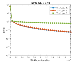
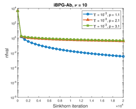
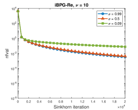
(a) $\nu=10$

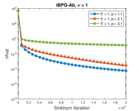
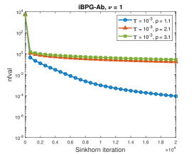
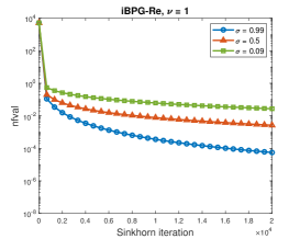
(b) $\nu=1$

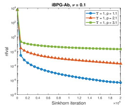
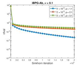
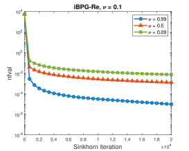
(c) $\nu=0.1$

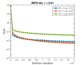
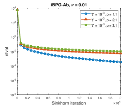
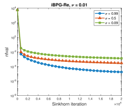
(d) $\nu=0.01$

Figure 1: Comparisons between iBPGM-Ab and iBPGM-Re under different choices of tolerance parameters for difference choices of $\nu$.

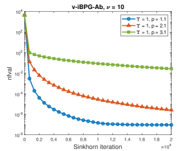
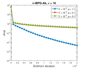
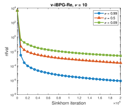
(a) $\nu=10$

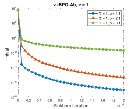
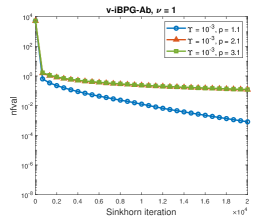
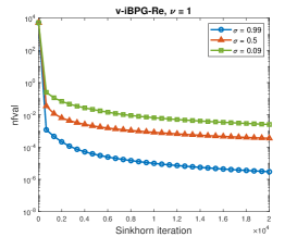
(b) $\nu=1$

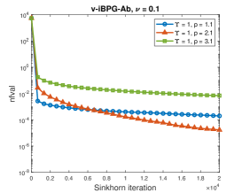
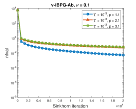
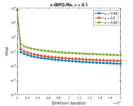
(c) $\nu=0.1$

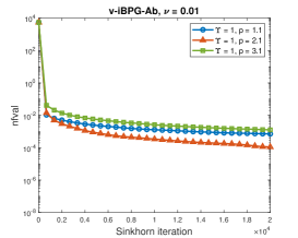
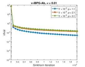
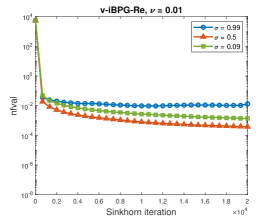
(d) $\nu=0.01$

Figure 2: Comparisons between v-iBPGM-Ab and v-iBPGM-Re under different choices of tolerance parameters for difference choices of $\nu$.

6 Concluding remarks

In this paper, we develop an inexact Bregman proximal gradient method (iBPGM) based on two types of two-point inexact stopping criteria, and establish the iteration complexity of $\mathcal{O}(1/k)$ as well as the convergence of the sequence under some proper conditions. To improve the convergence speed, we further develop an inertial variant of our iBPGM (denoted by v-iBPGM) and show that it has the iteration complexity of $\mathcal{O}(1/k^{\gamma})$, where $\gamma\geq 1$ is a restricted relative smoothness exponent. Thus, when $\gamma>1$, the v-iBPGM can improve the $\mathcal{O}(1/k)$ convergence rate of the iBPGM. We also conduct some preliminary numerical experiments for solving the discrete quadratic regularized optimal transport problem to show the convergence behaviors of the iBPGM and v-iBPGM under different inexactness settings.

Appendix A Proofs of supporting lemmas

A.1 Proof of Lemma 2.3

For any $\varepsilon>0$, we have from $\sum^{\infty}_{k=0}\alpha_{k}<\infty$ that there exists $\widetilde{N}\geq 0$ such that $\sum^{\infty}_{k=\widetilde{N}}\alpha_{k}\leq\varepsilon/2$. Now, let $N_{\varepsilon}:=\max\left\{\widetilde{N}+1,\,2\varepsilon^{-1}\sum^{\widetilde{N}-1}_{i=0}i\alpha_{i}\right\}$. Then, for any $k\geq N_{\varepsilon}$, we see that

$$\frac{1}{k}\sum^{k-1}_{i=0}i\alpha_{i}=\frac{1}{k}\sum^{\widetilde{N}-1}_{i=0}i\alpha_{i}+\frac{1}{k}\sum^{k-1}_{i=\widetilde{N}}i\alpha_{i}\leq\frac{1}{N_{\varepsilon}}\sum^{\widetilde{N}-1}_{i=0}i\alpha_{i}+\sum^{k-1}_{i=\widetilde{N}}\alpha_{i}\leq\varepsilon.$$

Since $\varepsilon$ is arbitrary, we can conclude that $\frac{1}{k}\sum^{k-1}_{i=0}i\alpha_{i}\to 0$.

A.2 Proof of Lemma 2.4

First, from condition (2.4), there exists $\bm{d}\in\partial_{\delta}P(\widetilde{\bm{x}}^{*})$ such that $\bm{d}+\nabla f(\bm{y})+\lambda(\nabla\phi(\bm{x}^{*})-\nabla\phi(\bm{y}))=\Delta$. Then, for any $\bm{x}\in\mathrm{dom}\,P\cap\mathrm{dom}\,\phi$, we see that

$$P(\bm{x})\geq P(\widetilde{\bm{x}}^{*})+\langle\bm{d},\,\bm{x}-\widetilde{\bm{x}}^{*}\rangle-\delta=P(\widetilde{\bm{x}}^{*})+\langle\Delta-\nabla f(\bm{y})-\lambda(\nabla\phi(\bm{x}^{*})-\nabla\phi(\bm{y})),\,\bm{x}-\widetilde{\bm{x}}^{*}\rangle-\delta,$$

which implies that

$$P(\widetilde{\bm{x}}^{*})\leq P(\bm{x})-\langle\nabla f(\bm{y}),\,\widetilde{\bm{x}}^{*}-\bm{x}\rangle+\lambda\langle\nabla\phi(\bm{x}^{*})-\nabla\phi(\bm{y}),\,\bm{x}-\widetilde{\bm{x}}^{*}\rangle+|\langle\Delta,\,\widetilde{\bm{x}}^{*}-\bm{x}\rangle|+\delta.$$ (A.1)

Note from the four points identity (2.3) that

$$\langle\,\nabla\phi(\bm{x}^{*})-\nabla\phi(\bm{y}),\,\bm{x}-\widetilde{\bm{x}}^{*}\,\rangle=\mathcal{D}_{\phi}(\bm{x},\,\bm{y})-\mathcal{D}_{\phi}(\bm{x},\,\bm{x}^{*})-\mathcal{D}_{\phi}(\widetilde{\bm{x}}^{*},\,\bm{y})+\mathcal{D}_{\phi}(\widetilde{\bm{x}}^{*},\,\bm{x}^{*})$$ (A.2)

Thus, combining (A.1) and (A.2), we obtain that

$$P(\widetilde{\bm{x}}^{*}) \leq P(\bm{x})-\langle\nabla f(\bm{y}),\,\widetilde{\bm{x}}^{*}-\bm{x}\rangle+\lambda\mathcal{D}_{\phi}(\bm{x},\,\bm{y})-\lambda\mathcal{D}_{\phi}(\bm{x},\,\bm{x}^{*})-\lambda\mathcal{D}_{\phi}(\widetilde{\bm{x}}^{*},\,\bm{y})$$ (A.3)

$$\qquad+\lambda\mathcal{D}_{\phi}(\widetilde{\bm{x}}^{*},\,\bm{x}^{*})+|\langle\Delta,\,\widetilde{\bm{x}}^{*}-\bm{x}\rangle|+\delta.$$

On the other hand, since $f$ is $L$-smooth relative to $\phi$ restricted on $\mathcal{X}$ (by Assumption A3) and $f$ is convex with $\mathrm{dom}\,f\supseteq\mathrm{dom}\,\phi$, then

$$f(\widetilde{\bm{x}}^{*}) \leq f(\bm{y})+\langle\nabla f(\bm{y}),\,\widetilde{\bm{x}}^{*}-\bm{y}\rangle+L\mathcal{D}_{\phi}(\widetilde{\bm{x}}^{*},\,\bm{y}),$$

$$f(\bm{x}) \geq f(\bm{y})+\langle\nabla f(\bm{y}),\,\bm{x}-\bm{y}\rangle.$$

Summing the above two inequalities, we obtain that

$$f(\widetilde{\bm{x}}^{*})\leq f(\bm{x})+\langle\nabla f(\bm{y}),\,\widetilde{\bm{x}}^{*}-\bm{x}\rangle+L\mathcal{D}_{\phi}(\widetilde{\bm{x}}^{*},\,\bm{y}).$$ (A.4)

Thus, summing (A.3) and (A.4), one can obtain the desirsed result.

A.3 Proof of Lemma 4.1

We first show by induction that $\theta_{k}\geq\frac{1}{k+\gamma}$ for all $k\geq 0$. This obviously holds for $k=0$ since $\theta_{0}=1$. Suppose that $\theta_{k}\geq\frac{1}{k+\gamma}$ holds for some $k\geq 0$. Since $0<\theta_{k}\leq 1$ and $\gamma\geq 1$, then $(1-\theta_{k})^{\gamma}\leq 1-\theta_{k}$. Using this and (4.3), we see that

$$\frac{(1-\theta_{k+1})^{\gamma}}{\theta_{k+1}^{\gamma}}\leq\frac{1}{\theta_{k}^{\gamma}}\quad\Longleftrightarrow\quad\frac{1-\theta_{k+1}}{\theta_{k+1}}\leq\frac{1}{\theta_{k}},$$

from which, we have that $\theta_{k+1}\geq\frac{\theta_{k}}{\theta_{k}+1}=\frac{1}{k+1+\gamma}$. This completes the induction. Using this fact, we further get

$$\quad\sum^{k}_{i=0}\frac{1}{\theta_{i-1}^{\gamma}}-\frac{1-\theta_{i}}{\theta_{i}^{\gamma}}=\frac{1}{\theta_{-1}^{\gamma}}-\frac{1}{\theta_{k}^{\gamma}}+\sum^{k}_{i=0}\frac{1}{\theta_{i}^{\gamma-1}}\leq 2+\sum^{k}_{i=1}\frac{1}{\theta_{i}^{\gamma-1}}$$

$$\leq 2+\sum^{k}_{i=1}(i+\gamma)^{\gamma-1}\leq 2+\int^{k+1}_{0}(t+\gamma)^{\gamma-1}\mathrm{d}t\leq 2+\frac{(k+1+\gamma)^{\gamma}}{\gamma}.$$

This completes the proof.

References

- [1] J. Altschuler, J. Weed, and P. Rigollet. Near-linear time approximation algorithms for optimal transport via Sinkhorn iteration. In Advances in Neural Information Processing Systems, volume 30, 2017.
- [2] J-F Aujol and Ch Dossal. Stability of over-relaxations for the forward-backward algorithm, application to FISTA. SIAM J. Optim., 25(4):2408–2433, 2015.
- [3] A. Auslender and M. Teboulle. Interior gradient and proximal methods for convex and conic optimization. SIAM J. Optim., 16(3):697–725, 2006.
- [4] H.H. Bauschke, J. Bolte, J. Chen, M. Teboulle, and X. Wang. On linear convergence of non-Euclidean gradient methods without strong convexity and Lipschitz gradient continuity. J. Optim. Theory Appl., 182(3):1068–1087, 2019.
- [5] H.H. Bauschke, J. Bolte, and M. Teboulle. A descent lemma beyond Lipschitz gradient continuity: First-order methods revisited and applications. Math. Oper. Res., 42(2):330–348, 2017.
- [6] H.H. Bauschke and J.M. Borwein. Legendre functions and the method of random Bregman projections. J. Convex Anal., 4(1):27–67, 1997.
- [7] H.H. Bauschke and J.M. Borwein. Joint and separate convexity of the Bregman distance. In Studies in Computational Mathematics, volume 8, pages 23–36. Elsevier, 2001.
- [8] H.H. Bauschke and P.L. Combettes. Convex Analysis and Monotone Operator Theory in Hilbert Spaces, volume 408. Springer, 2011.
- [9] A. Beck and M. Teboulle. Mirror descent and nonlinear projected subgradient methods for convex optimization. Oper. Res. Lett., 31(3):167–175, 2003.
- [10] A. Beck and M. Teboulle. A fast iterative shrinkage-thresholding algorithm for linear inverse problems. SIAM J. Imaging Sci., 2(1):183–202, 2009.
- [11] M. Blondel, V. Seguy, and A. Rolet. Smooth and sparse optimal transport. In International Conference on Artificial Intelligence and Statistics, volume 84, pages 880–889, 2018.
- [12] J. Bolte, S. Sabach, M. Teboulle, and Y. Vaisbourd. First order methods beyond convexity and Lipschitz gradient continuity with applications to quadratic inverse problems. SIAM J. Optim., 28(3):2131–2151, 2018.
- [13] S. Bonettini, F. Porta, and V. Ruggiero. A variable metric forward-backward method with extrapolation. SIAM J. Sci. Comput., 38(4):A2558–A2584, 2016.
- [14] S. Bonettini, S. Rebegoldi, and V. Ruggiero. Inertial variable metric techniques for the inexact forward-backward algorithm. SIAM J. Sci. Comput., 40(5):A3180–A3210, 2018.
- [15] L.M. Bregman. The relaxation method of finding the common point of convex sets and its application to the solution of problems in convex programming. USSR Comput. Math. Math. Phys., 7(3):200–217, 1967.
- [16] A. Chambolle and Ch Dossal. On the convergence of the iterates of the “fast iterative shrinkage/thresholding algorithm”. J. Optim. Theory Appl., 166(3):968–982, 2015.
- [17] H.-H. Chao and L. Vandenberghe. Entropic proximal operators for nonnegative trigonometric polynomials. IEEE Trans. Signal Process., 66(18):4826–4838, 2018.
- [18] H. Chu, L. Liang, K.-C. Toh, and L. Yang. An efficient implementable inexact entropic proximal point algorithm for a class of linear programming problems. Comput. Optim. Appl., 85(1):107–146, 2023.
- [19] P.L. Combettes and V.R. Wajs. Signal recovery by proximal forward-backward splitting. Multiscale Model. Simul., 4(4):1168–1200, 2005.
- [20] R.-A. Dragomir, A. Taylor, A. d’Aspremont, and J. Bolte. Optimal complexity and certification of Bregman first-order methods. Math. Program., 194(1-2):41–83, 2022.
- [21] M. Essid and J. Solomon. Quadratically regularized optimal transport on graphs. SIAM Journal on Scientific Computing, 40(4):A1961–A1986, 2018.
- [22] M. Fukushima and H. Mine. A generalized proximal point algorithm for certain non-convex minimization problems. Int. J. Syst. Sci., 12(8):989–1000, 1981.
- [23] D.H. Gutman and J.F. Peña. Perturbed Fenchel duality and first-order methods. Math. Program., 198(1):443–469, 2023.
- [24] F. Hanzely, P. Richtárik, and L. Xiao. Accelerated Bregman proximal gradient methods for relatively smooth convex optimization. Comput. Optim. Appl., 79(2):405–440, 2021.
- [25] L.T.K. Hien, D.N. Phan, N. Gillis, M. Ahookhosh, and P. Patrinos. Block Bregman majorization minimization with extrapolation. SIAM J. Math. Data Sci., 4(1):1–25, 2022.
- [26] K. Jiang, W. Si, C. Chen, and C. Bao. Efficient numerical methods for computing the stationary states of phase field crystal models. SIAM J. Sci. Comput., 42(6):B1350–B1377, 2020.
- [27] K. Jiang, D.F. Sun, and K.-C. Toh. An inexact accelerated proximal gradient method for large scale linearly constrained convex SDP. SIAM J. Optim., 22(3):1042–1064, 2012.
- [28] S. Kabbadj. Inexact version of Bregman proximal gradient algorithm. In Abstract and Applied Analysis, volume 2020, 2020.
- [29] G. Lan, Z. Lu, and R.D.C. Monteiro. Primal-dual first-order methods with iteration-complexity for cone programming. Math. Program., 126(1):1–29, 2011.
- [30] P.L. Lions and B. Mercier. Splitting algorithms for the sum of two nonlinear operators. SIAM J. Numer. Anal., 16(6):964–979, 1979.
- [31] D.A. Lorenz, P. Manns, and C. Meyer. Quadratically regularized optimal transport. Applied Mathematics & Optimization, 83:1919–1949, 2021.
- [32] H. Lu, M.R. Freund, and Y. Nesterov. Relatively smooth convex optimization by first-order methods, and applications. SIAM J. Optim., 28(1):333–354, 2018.
- [33] M.C. Mukkamala, P. Ochs, T. Pock, and S. Sabach. Convex-concave backtracking for inertial Bregman proximal gradient algorithms in nonconvex optimization. SIAM J. Math. Data Sci., 2(3):658–682, 2020.
- [34] Y. Nesterov. A method of solving a convex programming problem with convergence rate . Soviet Math. Dokl., 27(2):372–376, 1983.
- [35] Y. Nesterov. On an approach to the construction of optimal methods of minimization of smooth convex functions. Èkonom. i. Mat. Metody, 24:509–517, 1988.
- [36] Y. Nesterov. Introductory Lectures on Convex Optimization: A Basic Course, volume 87. Springer Science & Business Media, 2003.
- [37] Y. Nesterov. Smooth minimization of non-smooth functions. Math. Program., 103(1):127–152, 2005.
- [38] Y. Nesterov. Gradient methods for minimizing composite functions. Math. Program., 140(1):125–161, 2013.
- [39] G. Peyré and M. Cuturi. Computational optimal transport. Found. Trends Mach. Learn., 11(5-6):355–607, 2019.
- [40] B.T. Polyak. Introduction to Optimization. Optimization Software Inc., New York, 1987.
- [41] R.T. Rockafellar. Convex Analysis. Princeton University Press, Princeton, 1970.
- [42] M. Romain and A. d’Aspremont. A Bregman method for structure learning on sparse directed acyclic graphs. arXiv preprint arXiv:2011.02764, 2020.
- [43] M. Schmidt, N. Roux, and F. Bach. Convergence rates of inexact proximal-gradient methods for convex optimization. In Advances in Neural Information Processing Systems, volume 24, 2011.
- [44] F. Stonyakin, A. Tyurin, A. Gasnikov, P. Dvurechensky, A. Agafonov, D. Dvinskikh, M. Alkousa, D. Pasechnyuk, S. Artamonov, and V. Piskunova. Inexact model: A framework for optimization and variational inequalities. Optim. Methods Softw., 36(6):1155–1201, 2021.
- [45] M. Teboulle. A simplified view of first order methods for optimization. Math. Program., 170(1):67–96, 2018.
- [46] P. Tseng. On accelerated proximal gradient methods for convex-concave optimization. Technical report, 2008.
- [47] P. Tseng. Approximation accuracy, gradient methods, and error bound for structured convex optimization. Math. Program., 125(2):263–295, 2010.
- [48] Q. Van Nguyen. Forward-backward splitting with Bregman distances. Vietnam J. Math., 45(3):519–539, 2017.
- [49] S. Villa, S. Salzo, L. Baldassarre, and A. Verri. Accelerated and inexact forward-backward algorithms. SIAM J. Optim., 23(3):1607–1633, 2013.
- [50] L. Yang and K.-C. Toh. Bregman proximal point algorithm revisited: A new inexact version and its variant. SIAM J. Optim., 32(3):1523–1554, 2022.
- [51] Y. Zhou, Y. Liang, and L. Shen. A simple convergence analysis of Bregman proximal gradient algorithm. Comput. Optim. Appl., 73(3):903–912, 2019.