Raise a Child in Large Language Model:
Towards Effective and Generalizable Fine-tuning

Abstract

Recent pretrained language models extend from millions to billions of parameters. Thus the need to fine-tune an extremely large pretrained model with a limited training corpus arises in various downstream tasks. In this paper, we propose a straightforward yet effective fine-tuning technique, Child-Tuning, which updates a subset of parameters (called child network) of large pretrained models via strategically masking out the gradients of the non-child network during the backward process. Experiments on various downstream tasks in GLUE benchmark show that Child-Tuning consistently outperforms the vanilla fine-tuning by $1.5\sim 8.6$ average score among four different pretrained models, and surpasses the prior fine-tuning techniques by $0.6\sim 1.3$ points. Furthermore, empirical results on domain transfer and task transfer show that Child-Tuning can obtain better generalization performance by large margins.

1 Introduction

Pretrained Language Models (PLMs) have had a remarkable effect on the natural language processing (NLP) landscape recently (Devlin et al., 2019; Liu et al., 2019; Clark et al., 2020). Pretraining and fine-tuning have become a new paradigm of NLP, dominating a large variety of tasks.

Despite its great success, how to adapt such large-scale pretrained language models with millions to billions of parameters to various scenarios, especially when the training data is limited, is still challenging. Due to the extremely large capacity and limited labeled data, conventional transfer learning tends to aggressive fine-tuning (Jiang et al., 2020), resulting in: 1) degenerated results on the test data due to overfitting (Devlin et al., 2019; Phang et al., 2018; Lee et al., 2020), and 2) poor generalization ability in transferring to out-of-domain data or other related tasks (Mahabadi et al., 2021; Aghajanyan et al., 2021).

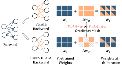
Figure 1: The illustration of Child-Tuning. Left: It forwards on the whole network while backwarding on a subset of network (i.e., child network). Right: To achieve this, a task-free or task-driven mask is performed on the gradients of the non-child network, resetting them to zero (grey diagonal grids).

Preventing the fine-tuned models to deviate too much from the pretrained weights (i.e., with less knowledge forgetting), is proved to be effective to mitigate the above challenges (Gouk et al., 2020). For instance, RecAdam (Chen et al., 2020) introduces $L_{2}$ distance penalty between the fine-tuned weights and their pretrained weights. In addition, Mixout (Lee et al., 2020) randomly replaces part of the model parameters with their pretrained weights during fine-tuning. The core idea behind them is to utilize the pretrained weights to regularize the fine-tuned model.

In this paper, we propose to mitigate the aggressive fine-tuning problem from a new perspective. Based on the observation that it is unnecessary to update all the parameters within the large-scale model during fine-tuning, we propose an effective fine-tuning technique, Child-Tuning, which straightforwardly updates a subset of parameters (called child network) via strategically masking out the gradients of non-child network in the backward process, as illustrated in Figure 1. Note that it is different from model pruning, since it still forwards on the whole network, thus making the full use of knowledge hidden in the pretrained weights.

In detail, we propose two variants, Child-Tuning_F and Child-Tuning_D, which respectively detect the child network in a task-free and a task-driven way. Child-Tuning_F chooses out the child network in the absence of task data via a Bernoulli distribution. It introduces noise to the full gradients, playing a role of regularization, hence preventing overfitting to small datasets and leading to better generalization. Furthermore, Child-Tuning_D utilizes the downstream task data to detect the most task-related parameters as the child network and freezes the parameters in non-child network to their pretrained weights. It decreases the hypothesis space of the model via a task-specific mask applied to the full gradients, helping to effectively adapt the large-scale pretrained model to various tasks and meanwhile greatly maintain its original generalization ability.

Our extensive experiments on the GLUE benchmark show that Child-Tuning can be more excellent at fine-tuning different PLMs, with up to $8.60$ average score improvement on CoLA/RTE/MRPC/STS-B tasks compared to vanilla fine-tuning (Section. 3.3). Moreover, it achieves better generalization ability in transferring to out-of-domain data and other related tasks (Section. 3.4). Experimental results also demonstrate that Child-Tuning yields consistently greater improvements than state-of-the-art fine-tuning methods. More importantly, since Child-Tuning is orthogonal to these prior methods, integrating Child-Tuning with them can even lead to further improvements (Section. 4.1).

In summary, our contributions are three-fold:

• We propose Child-Tuning, a straightforward yet effective fine-tuning technique that only updates the parameters in the child network. We explore to detect the child network in both task-free and task-driven ways.

• Child-Tuning can effectively adapt the large-scale pretrained model to various downstream scenarios, from in-domain to out-of-domain, and cross-task transfer learning.

• Since Child-Tuning is orthogonal to prior fine-tuning methods, integrating Child-Tuning with them can further boost the fine-tuning performance.

2 Methodology

To better adapt large-scale pretrained language model to various downstream tasks, we propose a simple yet effective fine-tuning technique, Child-Tuning. We firstly introduce a gradient mask in the backward process to achieve the aim of updating a subset of parameters (i.e., child network), while still utilizing the knowledge of the whole large model in the forward process (Section 2.1). Then, we explore two ways to detect the child network (i.e., generate different gradient masks): Child-Tuning_F that are in a task-free way (Section 2.2), and Child-Tuning_D that are in a task-driven way ( Section 2.3).

2.1 Overview of Child-Tuning

We start the introduction of Child-Tuning by giving a general formulation of the back propagation during the vanilla fine-tuning. We denote the parameters of the model at the $t$-th iteration as $\mathbf{w}_{t}$ ($\mathbf{w}_{0}$ refers to the pretrained weights). The vanilla fine-tuning computes the gradient of the loss $\mathcal{L}(\mathbf{w}_{t})$ and then applies gradient descent to all parameters, which can be formulated as:

$$\mathbf{w}_{t+1} =\mathbf{w}_{t}-\eta\frac{\partial\mathcal{L}(\mathbf{w}_{t})}{\partial\mathbf{w}_{t}}$$ (1)

where $\frac{\partial\mathcal{L}(\mathbf{w}_{t})}{\partial\mathbf{w}_{t}}$ are the gradients corresponding to the model parameters $\mathbf{w}_{t}$, $\eta$ is the learning rate.

Child-Tuning also backwardly computes the gradients of all trainable parameters like standard fine-tuning. However, the key difference is that Child-Tuning determines a child network $\mathcal{C}_{t}$ at the $t$-th iteration, and only updates this part of parameters. To achieve this, we firstly define a $0$-$1$ mask that is the same-sized as $\mathbf{w}$ as follows:

$${\color[rgb]{0.25,0.39453125,0.5859375}\bm{M}^{(i)}_{t}}=\left\{\begin{array}[]{lc}1,&\mathbf{w}^{(i)}_{t}\in\mathcal{C}_{t}\\ 0,&\mathbf{w}^{(i)}_{t}\notin\mathcal{C}_{t}\end{array}\right.$$ (2)

where $\bm{M}^{(i)}_{t}$ and $\mathbf{w}^{(i)}_{t}$ denote the $i$-th element of the mask $\bm{M}_{t}$ and parameters $\mathbf{w}_{t}$ at the $t$-th training iteration, respectively.

Then, we formally define Child-Tuning technique by simply replacing Eq. 1 with the following equation:

$$\mathbf{w}_{t+1}=\mathbf{w}_{t}-\eta\frac{\partial\mathcal{L}(\mathbf{w}_{t})}{\partial\mathbf{w}_{t}}\odot{\color[rgb]{0.25,0.39453125,0.5859375}\bm{M}_{t}}$$ (3)

Algorithm 1 Child-Tuning for Adam Optimizer

1:$\mathbf{w}_{0}$: initial pretrained weights; $\mathcal{L}(\mathbf{w})$: stochastic objective function with parameters $\mathbf{w}$; $\eta$: learning rate; $\beta_{1},\beta_{2}\in[0,1)$: exponential decay rates for the moment estimates;

2:initialize timestep $t\leftarrow 0$, first moment vector $m_{0}\leftarrow 0$, second moment vector $v_{0}\leftarrow 0$

3:while not converged do

4:     $t\leftarrow t+1$

5:      // Get gradients

6:     $\mathbf{g}_{t}\leftarrow\frac{\partial\mathcal{L}(\mathbf{w}_{t})}{\partial\mathbf{w}_{t}}$

7:      // Get task-free/task-driven child network

8:     $\mathcal{C}_{t}\leftarrow\text{GetChildNetwork}()$

9:      // Generate a corresponding gradient mask

10:     $\bm{M}_{t}\leftarrow\text{GenerateMask}(\mathcal{C}_{t})$

11:      // Employ mask for gradients

12:     $\mathbf{g}_{t}\leftarrow\mathbf{g}_{t}\odot\bm{M}_{t}$

13:     $\mathbf{m}_{t}\leftarrow\beta_{1}\cdot\mathbf{m}_{t-1}+(1-\beta_{1})\cdot\mathbf{g}_{t}$

14:     $\mathbf{v}_{t}\leftarrow\beta_{2}\cdot\mathbf{v}_{t-1}+(1-\beta_{2})\cdot\mathbf{g}^{2}_{t}$

15:      // Bias correction

16:     $\hat{\mathbf{m}}_{t}\leftarrow\mathbf{m}_{t}/(1-\beta_{1}^{t})$

17:     $\hat{\mathbf{v}}_{t}\leftarrow\mathbf{v}_{t}/(1-\beta_{2}^{t})$

18:      // Update weights

19:     $\mathbf{w}_{t}\leftarrow\mathbf{w}_{t-1}-\eta\cdot\hat{\bm{m}}_{t}/(\sqrt{\hat{\bm{v}}_{t}}+\epsilon)$

20:end while

21:return $\mathbf{w}_{t}$

Algorithm 1 provides the pseudo-code of Child-Tuning when applied to widely used Adam (Kingma and Ba, 2015) optimizer. The main difference is the insertion of line $5$-$7$.

2.2 Task-Free Variant: Child-Tuning_F

In this section, we firstly explore the choice of the child network that does not require any downstream task data, i.e., a task-free technique called Child-Tuning_F. Specifically, Child-Tuning_F generates a $0$-$1$ mask $\bm{M_{t}}$ at the $t$-th iteration drawn from a Bernoulli distribution with a probability $p_{F}$:

$$\bm{M}_{t}\sim\mathrm{Bernoulli}(p_{F})$$ (4)

The higher the $p_{F}$ is, the larger the child network is, and hence more parameters are updated. When $p_{F}=1$, Child-Tuning_F degenerates into the vanilla fine-tuning method. Note that we also enlarge the reserved gradients by $\frac{1}{p_{F}}$ to maintain the expectation of the gradients.

We theoretically justify the effectiveness of Child-Tuning_F. We denote $\mathbf{\Delta w}$ as the update at each iteration:

$$\mathbf{\Delta w}=\eta\frac{\partial\mathcal{L}(\mathbf{w})}{\partial\mathbf{w}}\odot\bm{M}$$ (5)

Intuitively, Theorem 1 shows the variance of gradients is a strictly decreasing function of $p_{F}$. Thus, Child-Tuning_F improves the variance of the gradients, and the trade-off between exploration and exploitation can be controlled by adjusting $p_{F}$. As illustrated in Theorem 2, with higher variance, the model can converge to more flat local minima (smaller $\rho$ in Theorem 2). Inspired by studies that show flat minima tends to generalize better (Keskar et al., 2017; Sun et al., 2020; Foret et al., 2021), we can further prove Child-Tuning_F decreases the generalization error bound.

Theorem 1.

Suppose $\mathcal{L}$ denotes the loss function on the parameter $\mathbf{w}$, the gradients obey a Gaussian distribution $\mathcal{N}(\frac{\partial\mathcal{L}}{\partial\mathbf{w}},\sigma^{2}_{\mathbf{g}}\mathbf{I}_{k})$, and SGD with learning rate $\eta$ is used. For a randomly sampled batch $\mathcal{B}$, if GradMask reserves gradients with probability $p_{F}$, the mean and covariance of the update $\mathbf{\Delta w}$ are,

$$\mathbb{E}[\mathbf{\Delta w}] =-\eta\frac{\partial\mathcal{L}}{\partial\mathbf{w}}$$ (6)

$$\Sigma[\mathbf{\Delta w}] =\frac{\eta^{2}\sigma_{\mathbf{g}}^{2}\mathbf{I}_{k}}{p_{F}|\mathcal{B}|}+\frac{(1-p_{F})\eta^{2}\text{diag}\{\frac{\partial\mathcal{L}}{\partial\mathbf{w}}\}^{2}}{p_{F}}$$ (7)

Specially, when $\mathbf{w}$ is a local minima, $\mathbb{E}[\mathbf{\Delta w}]=\mathbf{0}_{k},\Sigma[\mathbf{\Delta w}]=\sigma^{2}\mathbf{I}_{k}$ and $\sigma^{2}=\frac{\eta^{2}\sigma_{\mathbf{g}}^{2}}{p_{F}|\mathcal{B}|}$ is a strictly decreasing function of $p_{F}$.

Theorem 2.

Suppose $\mathbf{w}_{0}$ denotes the pretrained parameter; $k$ is the number of parameters; $\mathbf{w}$ denotes the local minima the algorithm converges to; $\rho$ is the greatest eigenvalue of the Hessian matrix on $\mathbf{w}$, which indicates the sharpness. If $\mathbf{\Delta w}\sim N(\mathbf{0}_{k},\sigma^{2}\mathbf{I}_{k})$, when the following bound holds, the algorithm can converge to the local minima $\mathbf{w}$ with high probability,

$$\rho\leq O\big{(}\frac{1}{\sigma^{2}}\big{)}$$ (8)

Suppose the prior over parameters after training is $P=N(\mathbf{w}_{0},\sigma_{0}^{2}\mathbf{I}_{k})$, the following generalization error bound holds with high probability,

(9)

where $\mathcal{R}$ is a term not determined by $\sigma$.

Thus, Child-Tuning_F can be viewed as a strong regularization for the optimization process. It enables the model to skip the saddle point in the loss landscape and encourages the model to converge to a more flat local minima. Please refer to Appendix E for more details about stated theorems and proofs.

2.3 Task-Driven Variant: Child-Tuning_D

Taking the downstream labeled data into consideration, we propose Child-Tuning_D, which detects the most important child network for the target task. Specifically, we adopt the Fisher information estimation to find the highly relevant subset of the parameters for a specific downstream task. Fisher information serves as a good way to provide an estimation of how much information a random variable carries about a parameter of the distribution (Tu et al., 2016a, b). For a pretrained model, Fisher information can be used to measure the relative importance of the parameters in the network towards the downstream tasks.

Formally, the Fisher Information Matrix (FIM) for the model parameters $\mathbf{w}$ is defined as follows:

where $\mathbf{x}$ and $y$ denote the input and the output respectively. It can be also viewed as the covariance of the gradient of the log likelihood with respect to the parameters $\mathbf{w}$. Following Kirkpatrick et al. (2016), given the task-specific training data data $D$, we use the diagonal elements of the empirical FIM to point-estimate the task-related importance of the parameters. Formally, we derive the Fisher information for the $i$-th parameter as follows:

$$\mathbf{F}^{(i)}\left(\mathbf{w}\right)=\frac{1}{\left|D\right|}\sum_{j=1}^{\left|D\right|}\left(\frac{\partial\log p\left(y_{j}|\mathbf{x}_{j};\mathbf{w}\right)}{\partial\mathbf{w}^{(i)}}\right)^{2}$$ (10)

We assume that the more important the parameter towards the target task, the higher Fisher information it conveys. Hence the child network $\mathcal{C}$ is comprised of the parameters with the highest information. The child network ratio is $p_{D}=\frac{\left|\mathcal{C}\right|}{\left|\mathcal{C}\right|+\left|\overline{\mathcal{C}}\right|}\in(0,1]$, where $\overline{\mathcal{C}}$ denotes the non-child network. As $p_{D}$ rises, the scale of the child network also increases, and when $p_{D}=1$ it degenerates into the vanilla fine-tuning strategy.

Method	BERT					XLNet
	CoLA	RTE	MRPC	STS-B	Avg	CoLA	RTE	MRPC	STS-B	Avg
Vanilla Fine-tuning	63.13	70.18	90.77	89.61	78.42	47.14	77.62	91.90	91.77	77.11
Child-TuningF	63.71	72.06	91.22	90.18	79.29	52.07	78.05	92.29	91.81	78.56
Child-TuningD	64.92	73.14	91.42	90.18	79.92	51.54	80.94	92.46	91.82	79.19
Method	RoBERTa					ELECTRA
	CoLA	RTE	MRPC	STS-B	Avg	CoLA	RTE	MRPC	STS-B	Avg
Vanilla Fine-tuning	66.10	85.20	92.62	92.04	83.99	47.42	88.23	92.95	81.86	77.62
Child-TuningF	65.99	84.80	92.66	92.15	83.90	62.31	88.41	93.09	91.73	83.89
Child-TuningD	66.71	86.14	92.78	92.36	84.50	70.62	88.90	93.32	92.02	86.22

Table 1: Comparison between Child-Tuning and vanilla fine-tuning applied to four widely used large-scale Pretrained Language Models (PLMs). Average scores on all tasks are underlined. The best results are bold. It shows that Child-Tuning yields consistent improvements across all tasks among different PLMs, especially for Child-Tuning_D that detects the child network in a task-driven way.

Since the overhead of obtaining the task-driven child network is heavier than that of the task-free one, we simply derive the child network for Child-Tuning_D at the beginning of fine-tuning, and keep it unchanged during the fine-tuning, i.e., $\mathcal{C}_{0}=\mathcal{C}_{1}=\dots=\mathcal{C}_{T}$. In this way, Child-Tuning_D dramatically decreases the hypothesis space of the large-scale models, thus alleviating overfitting. Meanwhile, keeping the non-child network freezed to their pretrained weights can substantially maintain the generalization ability.

3 Experiments

3.1 Datasets

GLUE benchmark

Following previous studies (Lee et al., 2020; Dodge et al., 2020), we conduct experiments on various datasets from GLUE leaderboard (Wang et al., 2019), including linguistic acceptability (CoLA), natural language inference (RTE, QNLI, MNLI), paraphrase and similarity (MRPC, STS-B, QQP), and sentiment classification (SST-2). CoLA and SST-2 are single-sentence classification tasks and the others are involved with a pair of sentences. The detailed statistics and metrics are provided in Appendix A. Following most previous works (Phang et al., 2018; Lee et al., 2020; Dodge et al., 2020), we fine-tune the pretrained model on the training set and directly report results on the dev set using the last checkpoint, since the test results are only accessible by the leaderboard with a limitation of the number of submissions.

NLI datasets

In this paper, we also conduct experiments to explore the generalization ability of the fine-tuned model based on several Natural Language Inference (NLI) tasks. Specifically, we additionally introduce three NLI datasets, i.e., SICK (Marelli et al., 2014), SNLI (Bowman et al., 2015) and SciTail (Khot et al., 2018). We also report results on the dev set consistent with GLUE.

3.2 Experiments Setup

We use the pretrained models and codes provided by HuggingFace (Wolf et al., 2020), and follow their default hyperparameter settings unless noted otherwise. Appendix B provides detailed experimental setups (e.g., batch size, training steps, and etc.) for BERT_LARGE (Devlin et al., 2019), XLNet_LARGE Yang et al. (2019), RoBERTa_LARGE Liu et al. (2019), and ELECTRA_LARGE Clark et al. (2020). We report the averaged results over $10$ random seeds.

Datasets	MNLI					SNLI
	Vanilla	C.TuningF	$\Delta_{F}$	C.TuningD	$\Delta_{D}$	Vanilla	C.TuningF	$\Delta_{F}$	C.TuningD	$\Delta_{D}$
MNLI	75.30	75.95	+0.65	76.61	+1.31	65.80	66.01	+0.21	66.82	+1.02
MNLI–m	76.50	77.79	+1.29	77.98	+1.48	67.71	67.27	–0.44	68.48	+0.77
SNLI	69.61	70.35	+0.74	71.17	+1.56	82.90	83.17	+0.27	83.66	+0.76
SICK	48.25	49.13	+0.88	50.15	+1.90	51.50	51.16	–0.34	51.42	–0.08
SciTail	73.65	75.42	+1.77	75.08	+1.43	69.35	70.74	+1.39	71.10	+1.75
QQP	71.37	72.24	+0.87	72.67	+1.30	70.60	71.52	+0.92	71.19	+0.59
Avg∗	67.88	68.99	+1.11	69.41	+1.53	64.99	65.34	+0.35	65.80	+0.81

Table 2: Probing domain generalization. The models are trained on MNLI/SNLI and tested on out-of-domain data. $\Delta_{F}$ and $\Delta_{D}$ denotes the improvement of C.Tuning_F and C.Tuning_D compared with vanilla fine-tuning. Average scores (marked with ^∗) is computed excluding in-domain results (underlined). Positive transfer results are highlighted in blue. Child-Tuning can better maintain the out-of-domain generalization ability of the model.

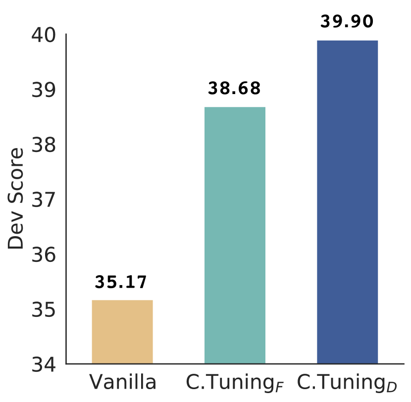
(a) CoLA (Matthews Corr)

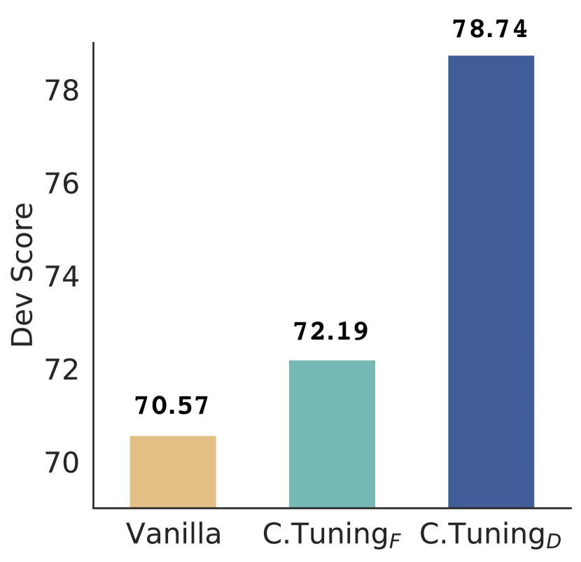
(b) STS-B (Spearman Corr)

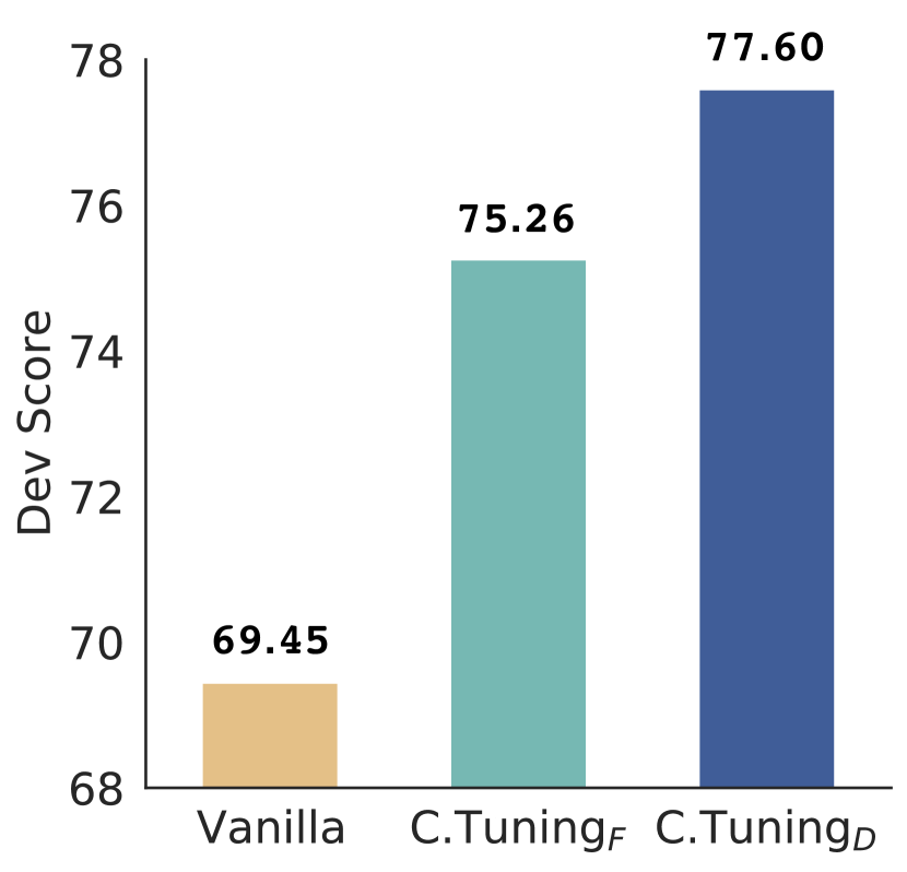
(c) QNLI (Accuracy)

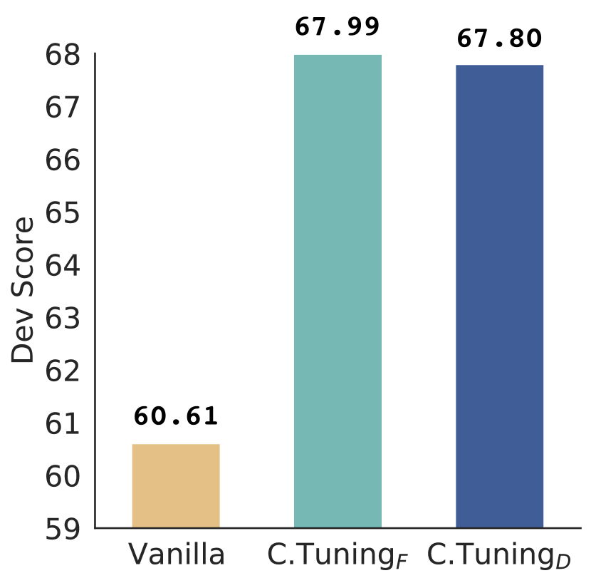
(d) QQP (F1)

Figure 2: Probing task generalization. The model is fine-tuned on MRPC task and transferred to four different tasks. Child-Tuning can maintain more generalizable representations compared with vanilla fine-tuning.

3.3 Results on GLUE Benchmark

In this section, we show the results of four widely used large PLMs on four GLUE tasks: CoLA, RTE, MRPC, and STS-B, following Lee et al. (2020). Besides vanilla fine-tuning, we also report the results of two variants of Child-Tuning, including both Child-Tuning_F $\left(p_{F}={0.2,0.3,0.4}\right)$ and Child-Tuning_D $\left(p_{D}={0.1,0.2,0.3}\right)$.

As Table 1 illustrates, Child-Tuning outperforms vanilla fine-tuning by a large gain across all the tasks on different PLMs. For instance, Child-Tuning yields an improvement of up to $2.08$ average score on XLNet, and $8.60$ average score on ELECTRA. Besides, the straightforward task-free variant, Child-Tuning_F, can still provide an improvement of $0.87$ average score on BERT and $6.27$ on ELECTRA. Child-Tuning_D, which detects child network in a task-driven way, is more aware of the unique characteristics of the downstream task, and therefore achieves the best performance, with up to $1.50$ and $8.60$ average score improvement on BERT and ELECTRA. In summary, we can come to a conclusion that Child-Tuning is model-agnostic and can consistently outperform vanilla fine-tuning on different PLMs.

3.4 Probing Generalization Ability of the Fine-tuned Model

To measure the generalization properties of various fine-tuning methods, in this section, we conduct probing experiments from two aspects, that is, domain generalization and task generalization.

3.4.1 Domain Generalization

Besides boosting performance on the target downstream task, we also expect Child-Tuning can help the fine-tuned model achieve better generalization ability towards out-of-domain data.

We evaluate how well the fine-tuned model generalizes to out-of-domain data based on several Natural Language Inference (NLI) tasks. In detail, we fine-tune BERT_LARGE with different strategies on $5k$ subsampled MNLI and SNLI datasets respectively, and directly test the accuracy of the fine-tuned models on other NLI datasets in different domains, including MNLI, MNLI-mismatch, SNLI, SICK, SciTail, and QQP. As Table 2 illustrates, Child-Tuning outperforms vanilla fine-tuning across different out-of-domain datasets. Specifically, Child-Tuning_F improves $1.11$/$0.35$ average score for models trained on MNLI/SNLI, while Child-Tuning_D improves up to $1.53$/$0.81$ average score. In particular, Child-Tuning_D achieves $1.90$ score improvement on SICK task and $1.56$ on SNLI task for models trained on MNLI.

The results suggest that Child-Tuning encourages the model to learn more general semantic features during fine-tuning, rather than some superficial features unique to the training data. Hence, the fine-tuned model can well generalize to different datasets, even though their domains are quite different from the dataset the model is trained on.

Methods	CoLA	RTE	MRPC	STS-B	Avg	$\Delta$
Vanilla Fine-tuning†	60.60 (   –   )	70.40 (   –   )	88.00 (   –   )	90.00 (   –   )	77.25	–
Vanilla Fine-tuning	63.13 (64.31)	70.18 (72.56)	90.77 (91.42)	89.61 (90.12)	78.42	0.00
Weight Decay Daumé III (2007)	63.63 (64.56)	71.99 (74.37)	90.93 (91.70)	89.82 (90.29)	79.09	+0.67
Top-$K$ Tuning Houlsby et al. (2019)	62.63 (64.06)	70.90 (74.73)	91.09 (92.20)	89.97 (90.15)	78.65	+0.23
Mixout Lee et al. (2020)	63.60 (64.82)	72.15 (75.45)	91.29 (91.85)	89.99 (90.13)	79.26	+0.84
RecAdam Chen et al. (2020)	64.33 (65.33)	71.63 (73.29)	90.85 (92.01)	89.86 (90.42)	79.17	+0.75
R3F Aghajanyan et al. (2021)	64.13 (66.32)	72.28 (74.73)	91.18 (91.57)	89.61 (90.12)	79.30	+0.88
Child-TuningF	63.71 (66.06)	72.06 (74.73)	91.22 (91.85)	90.18 (90.92)	79.29	+0.87
Child-TuningD	64.92 (66.03)	73.14 (76.17)	91.42 (92.17)	90.18 (90.64)	79.92	+1.50
Child-TuningD + R3F	65.18 (66.03)	73.43 (76.17)	92.23 (92.65)	90.18 (90.64)∗	80.26	+1.84

Table 3: Comparison between Child-Tuning with other fine-tuning methods. We report the mean (max) results of $10$ random seeds. Results with ^† are taken from Yang et al. (2019), and others are from our implementation. The task-driven variant, Child-Tuning_D, achieves the best performance compared with other methods. Integrating Child-Tuning_D with other fine-tuning methods like R3F can yield further improvements. Note that since R3F is not applicable to regression task, the result on STS-B (marked with ^∗) is the same as Child-Tuning_D.

3.4.2 Task Generalization

To justify the generalization ability of the model from another perspective, we follow the probing experiments from  Aghajanyan et al. (2021), which first freezes the representations from the model trained on one task and then only trains a linear classifier on top of the model for another task.

In particular, we fine-tune BERT_LARGE on MRPC task, and transfer to four other GLUE tasks, i.e., CoLA, STS-B, QNLI, and QQP. As Figure 2 shows, Child-Tuning consistently outperforms vanilla fine-tuning on different transferred tasks. Compared with vanilla fine-tuning, Child-Tuning_F improves $4.58$ average score ($58.95\rightarrow 63.53$), while Child-Tuning_D even gains up to $7.06$ average score improvement ($58.95\rightarrow 66.01$).

In summary, fine-tuning with Child-Tuning gains better performance when the fine-tuned model is transferred to another task, demonstrating that Child-Tuning can maintain more generalizable representations produced by the model than vanilla fine-tuning.

4 Analysis and Discussion

4.1 Comparison with Prior Methods

In this section, we review and compare prior studies towards effective fine-tuning: 1) Weight Decay (Daumé III, 2007), which adds the $\lambda\|\mathbf{w}-\mathbf{w}_{0}\|_{2}$ penalty to the loss function, where $\mathbf{w}_{0}$ denotes the pretrained weights; 2) Top-$K$ Tuning, which only fine-tune the top-$K$ layers of the model with other layers freezed.  Houlsby et al. (2019) uses it as a strong baseline; 3) Mixout (Lee et al., 2020), which randomly replaces the parameters with their pretrained weights; 4) RecAdam (Chen et al., 2020), which is similar to Weight Decay while its loss weights $\lambda$ keeps changing during fine-tuning; 5) Robust Representations through Regularized Finetuning (R3F) (Aghajanyan et al., 2021), which is rooted in trust region theory. Appendix C shows detailed hyperparameter settings.

We compare Child-Tuning with these methods based on BERT_LARGE, and report the mean (max) score results in Table 3, following  Lee et al. (2020). While all the fine-tuning methods can bring improvements across four different tasks compared with vanilla fine-tuning, Child-Tuning achieves the best performance. In detail, among prior fine-tuning methods, Mixout and R3F yield the highest improvement with $0.84$ and $0.88$ average score respectively. Child-Tuning_F has performance on par with Mixout and R3F, while Child-Tuning_D achieves $1.50$ average score improvement in total. More importantly, Child-Tuning is flexible and orthogonal to most fine-tuning methods. Thus, integrating Child-Tuning with other methods can further boost the performance. For instance, combining Child-Tuning_D with R3F leads to a $1.84$ average score improvement in total.

In short, compared with prior fine-tuning methods, we find that 1) Child-Tuning is more effective in adapting PLMs to various tasks, especially for the task-driven variant Child-Tuning_D, and 2) Child-Tuning has the advantage that it is flexible enough to integrate with other methods to potentially achieve further improvements.

4.2 Results in Low-resource Scenarios

Dataset	Vanilla	C.TuningF	C.TuningD
CoLA	47.48	48.44	50.37
RTE	65.09	65.52	68.09
MRPC	84.91	85.44	86.49
STS-B	81.86	82.25	82.76
SST2	90.25	90.34	90.39
QNLI	81.68	83.09	83.42
QQP	71.30	72.15	71.79
MNLI	55.72	62.47	62.93
Avg	72.29	73.71	74.53

Table 4: Results in low-resource scenarios. Child-Tuning is better than vanilla fine-tuning in alleviating overfitting problems.

Fine-tuning a large pretrained model on extremely small datasets can be very challenging since the risk of overfitting rises (Dodge et al., 2020). Thus, in this section, we explore the effect of Child-Tuning with only a few training examples. To this end, we downsample all datasets in GLUE to $1$k training examples and fine-tune BERT_LARGE on them.

As Table 4 demonstrates, compared with vanilla fine-tuning, Child-Tuning_F improves the average score by $1.42$, and the improvement is even larger for Child-Tuning_D, which is up to $2.24$. It suggests that although overfitting is quite severe when the training data is in extreme low-resource scenarios, Child-Tuning can still effectively improve the model performance, especially for Child-Tuning_D since it decreases the hypothesis space of the model.

4.3 What is the Difference Between Child-Tuning and Model Pruning?

Child-Tuning_D detects the most important child network in a task-driven way, and only updates this parameters within the child network during the fine-tuning with other parameters freezed. It is very likely to be confused with model pruning (Li et al., 2017; Zhu and Gupta, 2018; Lin et al., 2020), which also detects a subnetwork within the model (but then removes the other parameters).

Actually, Child-Tuning and model pruning are different in both the objectives and methods. Regarding objectives, model pruning aims at improving the inference efficiency and maintaining the performance at the same time, while Child-Tuning is proposed to address the overfitting problem and improve the generalization ability for large-scale language models during fine-tuning. Regrading methods, model pruning abandons the unimportant parameters during inference, while the parameters that do not belong to the child network are still reserved for Child-Tuning during training and inference. In this way, the knowledge of the non-child network hidden in the pretrained weights will be fully utilized.

To better illustrate the effectiveness of Child-Tuning_D compared to model pruning, we set all the parameters not belonging to the child network to zero, which is referred to as Prune in Table 5. It shows that, once we abandon parameters out of the child network, the score dramatically decreases by $33.89$ points averaged on four tasks (CoLA/RTE/MRPC/STS-B), and the model even collapses on CoLA task. It also suggests that besides parameters in child network, those in the non-child network are also necessary since they can provide general knowledge learned in pretraining.

Methods	CoLA	RTE	MRPC	STS-B
Vanilla	63.13	70.18	90.77	89.61
Prune	0.00	51.12	81.40	45.63
Random	63.23	70.69	90.83	89.67
Lowest Info.	60.33	59.86	83.82	88.52
C.TuningD	64.92	72.78	91.26	90.18

Table 5: Ablation study of Child-Tuning_D. Prune: Abandon parameters out of the child network. Random: Randomly choose a child network and keep it unchanged during fine-tuning. Lowest Info.: Detect a child network with lowest Fisher information instead.

4.4 Is the Task-Driven Child Network Really that Important to the Target Task?

Child-Tuning_D detects the task-specific child network by means of choosing parameters with the highest Fisher information towards the downstream task data. In this section, we exlore whether the detected task-driven child network is really that important to the task.

To this end, we introduce two ablation studies for Child-Tuning_D: 1) Random: We randomly choose a child network and keep it unchanged during fine-tuning; 2) Lowest Info.: We choose those parameters with lowest Fisher information as the child network, contrasted to the highest Fisher information adopted in Child-Tuning_D.

As shown in Table 5, choosing the child network randomly can even outperform vanilla fine-tuning, with $0.18$ average score improvement. It supports our claim that there is no need to update all parameters of the large PLMs, and decreasing the hypothesis space can reduce the risk of overfitting. However, it is still worth finding a proper child network to further boost the performance. If we choose parameters with the lowest Fisher information (Lowest Fisher), the average score is dramatically decreased by $6.65$ compared with choosing with the highest Fisher information adopted in Child-Tuning_D. Hence, we can conclude that the child network detected by Child-Tuning_D is indeed important to the downstream task.

4.5 What is the Relationship among Child Networks for Different Tasks?

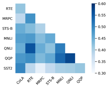
Figure 3: The overlapping ratio among task-driven child networks among GLUE tasks.

As the task-driven child networks are correlated with the tasks, we further explore the relationship among child networks for different tasks. To this end, we visualize the overlapping rate among different task-driven child networks, where we use the Jaccard similarity coefficient, $\frac{\left|\mathcal{C}^{i}\cap\mathcal{C}^{j}\right|}{\left|\mathcal{C}^{i}\cup\mathcal{C}^{j}\right|}$, to calculate the overlapping rate between task $i$ and $j$.

Figure 3 shows the overlap among GLUE tasks. As we expected, similar tasks tend to have higher overlapping ratios of child network. For example, the overlapping ratio among NLI tasks is remarkably higher than others, such as RTE and QNLI, QNLI and MNLI. For different kinds of tasks, their overlapping ratio is relatively lower, such as CoLA and MRPC. It is also interesting to find that the task-driven child network for SST2 overlaps less with other tasks except CoLA, even though SST2 and CoLA is not so similar. The reason may be that both SST2 and CoLA belongs to a single sentence classification task, while others are in a different format of sentence-pair classification tasks.

5 Related Work

Explosion of PLMs.

There has been an explosion of studies on Pretrained Language Models (PLMs). Devlin et al. (2019) propose BERT that is pretrained on large quantities of unannotated corpus with self-supervised tasks. Many PLMs also emerged such as GPT-$2$ Radford et al. (2018), GPT-$3$ Brown et al. (2020), ELECTRA (Clark et al., 2020), XLNet (Yang et al., 2019), RoBERTa (Liu et al., 2019), and BART (Lewis et al., 2020). The number of parameters of PLMs also explodes. BERT_LARGE has $340$ millions of parameters, and the number for GPT-$3$ is even up to $175$ billions.

Effective and generalizable fine-tuning.

With a mass of parameters, fine-tuning large PLMs tend to achieve degenerated performance due to overfitting and have poor generalization ability, especially on small datasets (Devlin et al., 2019; Phang et al., 2018; Lee et al., 2020). Therefore, different fine-tuning techniques have been proposed. Some of them utilize the pretrained weights to regularize the deviation of the fine-tuned model (Lee et al., 2020; Daumé III, 2007; Chen et al., 2020), while others compress the output information (Mahabadi et al., 2021) or injects noise into the input (Jiang et al., 2020; Aghajanyan et al., 2021). Moreover, Zhang et al. (2021) and Mosbach et al. (2021) point out that the omission of bias correction in the Adam optimizer used in Devlin et al. (2019) is also responsible for the degenerated results. Orthogonal to these methods, Child-Tuning address the problems by detecting the child network within the model in a task-free or task-driven way. It only updates parameters within the child network via a gradient mask, which is proved to be effective in adapting large PLMs to various tasks, along with better generalization ability.

Parameter-efficient Fine-tuning.

There are also studies focusing on parameter-efficient fine-tuning, for example, the adapter-based methods (Houlsby et al., 2019; Pfeiffer et al., 2020; Karimi Mahabadi et al., 2021), and the Diff-Pruning method (Guo et al., 2021). However, our Child-Tuning is different from this line of works. Firstly, they aim at fine-tuning as few as possible parameters to maintain performance, while we target effective and generalizable fine-tuning. Secondly, Diff-Pruning sparsifies diff-vector with gradient estimators, and adapter-based methods fine-tune new added module during training, while we detect the child network inside the model without extra parameters and only need to calculate the FIM before training for Child-Tuning_D. Finally, we consistently outperform vanilla fine-tuning by a large margin, while they achieve competitive performance with full model training.

6 Conclusion

To mitigate the overfitting problem and improve generalization for fine-tuning large-scale PLMs, we propose a straightforward yet effective fine-tuning technique, Child-Tuning, which only updates the child network during fine-tuning via strategically masking out the gradients of the non-child network. Two variants are introduced, Child-Tuning_F and Child-Tuning_D, which detect the child network in a task-free and task-driven way, respectively. Extensive experiments on various downstream tasks show that both of them can outperform vanilla fine-tuning and prior works by large gains among four different pretrained language models, and meanwhile largely enhance the generalization ability of the fine-tuned models. Since Child-Tuning is orthogonal to most prior fine-tuning techniques, integrating Child-Tuning with them can further boost the performance.

Appendix A GLUE Benchmark Introduction

In this paper, we conduct experiments on $8$ datasets in GLUE benchmark (Wang et al., 2019) as shown in Table 6, including single-sentence tasks, inference tasks, and similarity and paraphrase tasks. Note that the original GLUE benchmark includes $9$ different datasets in total. However, there are some issues with the construction of the WNLI dataset. Therefore most studies exclude this dataset (Devlin et al., 2019; Dodge et al., 2020) and we follow them. The metrics we report for each dataset are also illustrated in Table 6.

Dataset	#Train	#Dev	Metrics
Single-sentence Tasks
CoLA	8.5k	1.0k	Matthews Corr
SST-2	67k	872	Accuracy
Inference
RTE	2.5k	277	Accuracy
QNLI	105k	5.5k	Accuracy
MNLI	393k	9.8k	Accuracy
Similarity and Paraphrase
MRPC	3.7k	408	F1
STS-B	5.7k	1.5k	Spearman Corr
QQP	364k	40k	F1

Table 6: Statistics and metrics of eight datasets used in this paper form GLUE benchmark.

Appendix B Settings for Different Pretrained Language Models

In this paper, we fine-tune different large pretrained language models with Child-Tuning, including BERT_LARGE, XLNet_LARGE, RoBERTa_LARGE, and ELECTRA_LARGE. The training epochs/steps, batch size, and warmup steps are listed in Table 7. We use AdamW (Loshchilov and Hutter, 2019) optimizer, and set $\beta_{1}=0.9$, $\beta_{2}=0.999$, $\epsilon=1\text{e-}6$. We clip the gradients with a maximum norm of $1$, and the maximum sequence length is set as $128$. For Child-Tuning_F, we uses $p_{F}=\left\{0.2,0.3,0.4\right\}$ and re-scale the gradients to ensure the gradients after Child-Tuning_F are unbiased. For Child-Tuning_D, we use $p_{D}=\left\{0.1,0.2,0.3\right\}$. We use grid search for learning rate from $\left\{1\text{e-}5,2\text{e-}5,\dots,1\text{e-}4\right\}$. We conduct all the experiments on a single GTX-3090 GPU.

Model	Dataset	Batch Size	Training Epochs/Steps	Warmup Ratio/Steps
BERT	all	16	3 epochs	10%
XLNet	CoLA	128	1200 steps	120 steps
	RTE	32	800 steps	200 steps
	MRPC	32	800 steps	200 steps
	STS-B	32	3000 steps	500 steps
RoBERTa	CoLA	16	5336 steps	320 steps
	RTE	16	2036 steps	122 steps
	MRPC	16	2296 steps	137 steps
	STS-B	16	3598 steps	214 steps
ELECTRA	CoLA	32	3 epochs	10%
	RTE	32	10 epochs	10%
	MRPC	32	3 epochs	10%
	STS-B	32	10 epochs	10%

Table 7: Hyperparameters settings for different pretrained models on variant tasks. These settings are reported in the their official repository for best practice.

These pretrained models are all Transformer-based. XLNet (Yang et al., 2019) is an autoregressive pretrained language model with token permutations. It generates tokens in an autoregressive way while can still capture bidirectional context information. RoBERTa (Liu et al., 2019) is a robustly optimized version of BERT. It uses a dynamic masking mechanism, larger batch size, and longer training times, and it also abandons the next sentence prediction task. ELECTRA (Clark et al., 2020) pretrains the model with a generator and a discriminator. The discriminator is trained to distinguish whether the token is generated by the generator or the original token.

Appendix C Settings for Other Fine-tuning Methods

We compare Child-tuning with several other regularization approaches in our paper. In this section, we simply introduce these approaches and their hyperparameters settings.

Weight Decay

Daumé III (2007) proposes to adds a penalty item to the loss function to regulate the $L_{2}$ distance between fine-tuned models and the pretrained models. Therefore, the loss function is as follows:

$$\mathcal{L}(\mathbf{w})=\mathcal{L}_{\mathrm{CE}}(\mathbf{w})+\lambda_{\mathrm{WD}}\|\mathbf{w}-\mathbf{w}_{0}\|_{2}]$$

We grid search the optimal $\lambda_{\mathrm{WD}}$ from $\left\{10,1,10^{-1},10^{-2},10^{-3},10^{-4}\right\}$.

Top-$K$ Fine-tuning

Top-$K$ Fine-tuning is a common method and Houlsby et al. (2019) uses it as a strong baseline. Top-$K$ Fine-tuning only updatess the top $K$ layers along with the classification layer, while freezing all the other bottom layers. We grid search the optimal $K$ from $\left\{0,3,6,12\right\}$ in our paper.

Mixout

Lee et al. (2020) randomly replace the parameters with its pretrained weights with a certainly probability $p$ during fine-tuning, which aims to minimize the deviation of the fine-tuned model towards the pretrained weights. In our paper, we grid search the optimal $p$ from $\left\{0.1,0.2,\dots,0.8\right\}$. We use the implementation in https://github.com/bloodwass/mixout.

RecAdam

Chen et al. (2020) proposes a new optimizer RecAdam for fine-tuning, which can be considered as an advanced version of Weight Decay, because the coefficient of two different loss items are changed as the training progresses. The following equations demonstrate the new loss function, where $k$ and $t_{0}$ are controlling hyperparameters and $t$ is the current training step.

$$\mathcal{L}(\mathbf{w}) =\lambda_{\mathrm{Rec}}(t)\mathcal{L}_{\mathrm{CE}}(\mathbf{w})$$

$$+(1-\lambda_{\mathrm{Rec}}(t))\|\mathbf{w}-\mathbf{w}_{0}\|_{2}$$

$$\lambda_{\mathrm{Rec}}(t)=\frac{1}{1+\exp(-k\cdot(t-t_{0}))}$$

We grid search the $k$ from $\left\{0.05,0.1,0.2,0.5,1.0\right\}$, and $t_{0}$ from $\left\{50,100,250,500\right\}$. We use the implementation in https://github.com/Sanyuan-Chen/RecAdam.

Robust Representations through Regularized Fine-tuning (R3F)

Aghajanyan et al. (2021) propose R3F for fine-tuning based on trust region theory, which adds noise into the sequence input embedding and tries to minimize the symmetrical KL divergence between probability distributions given original input and noisy input. The loss function of R3F is as follows:

$$\mathcal{L}(\mathbf{w}) =\mathcal{L}_{\mathrm{CE}}(\mathbf{w})+\lambda_{\mathrm{R3F}}KL_{S}(f(x)||f(x+z))$$

$$s.t. \quad z\sim\mathcal{N}(0,\sigma^{2}I)\quad or\quad z\sim\mathcal{U}(-\sigma,\sigma)$$

where $f(\cdot)$ denotes the model and $z$ denotes the noise sampled from either normal distribution or uniform distribution controlled by hyperparameter $\sigma$, and $KL_{S}(x||y)=KL(x||y)+KL(y||x)$. We use both normal and unform distribution, $\lambda_{\mathrm{R3F}}=1$, and grid search the $\sigma$ from $\left\{0.1,0.5,1.0,5.0\right\}$. We use the implementation in https://github.com/pytorch/fairseq/tree/master/examples/rxf.

Appendix D Label Mapping in Task Generalization

MNLI and SNLI datasets contain three labels, i.e., entailment, neutral, and contradiction. For SciTail, it only has two labels, entailment and neutral, and therefore we map both neutral and contradiction in source label space to neutral in target label space following Mahabadi et al. (2021). For QQP, it has two labels, duplicate and not duplicate, and  Gong et al. (2018) interpret them as entailment and neutral respectively. We follow  Gong et al. (2018) and use the same mapping strategy as SciTail.

Appendix E Theoretical Details

We theoretically justify the effectiveness of Child-Tuning_F. Assume Child-Tuning_F reserves gradients with probability $p_{F}\in\left(0,1\right]$, and we simply use $p$ to denote $p_{F}$ in the following content. Theorem 1 shows the variance of gradients is a strictly decreasing function of $p$. When $p=1$, it degenerates into normal fine-tuning methods. Therefore, Child-Tuning_F can improve the variance of the gradients of the model. Next, Theorem 2 shows that with higher variance, the model can converge to more flat local minima (smaller $\rho$ in Theorem 2). Inspired by studies that show flat minima tends to generalize better (Keskar et al., 2017; Sun et al., 2020; Foret et al., 2021), we can further prove Child-Tuning_F decreases the generalization error bound.

Theorem 1.

Suppose $\mathcal{L}$ denotes the loss function on the parameter $\mathbf{w}$, for multiple data instances in the training set $\mathbf{x}\sim\mathcal{S}$, the gradients obey a Gaussian distribution $\mathcal{N}(\frac{\partial\mathcal{L}}{\partial\mathbf{w}},\sigma^{2}_{\mathbf{g}}\mathbf{I}_{k})$. For a randomly sampled batch $\mathcal{B}\sim\mathcal{S}$, when the learning algorithm is SGD with learning rate $\eta$, the reserving probability of the Child-Tuning_F is $p$, then the mean and covariance of the update $\mathbf{\Delta w}$ are,

$$\mathbb{E}[\mathbf{\Delta w}] =-\eta\frac{\partial\mathcal{L}}{\partial\mathbf{w}}$$ (11)

$$\Sigma[\mathbf{\Delta w}] =\frac{\eta^{2}\sigma_{\mathbf{g}}^{2}\mathbf{I}_{k}}{p|\mathcal{B}|}+\frac{(1-p)\eta^{2}\text{diag}\{\frac{\partial\mathcal{L}}{\partial\mathbf{w}}\}^{2}}{p}$$ (12)

where $\Sigma$ is the covariance matrix and diag$(\mathbf{x})$ is the diagonal matrix of the vector $\mathbf{x}$.

Specially, when $\mathbf{w}$ is a local minima, $\mathbb{E}[\mathbf{\Delta w}]=\mathbf{0}_{k},\Sigma[\mathbf{\Delta w}]=\sigma^{2}\mathbf{I}_{k}$ and $\sigma^{2}=\frac{\eta^{2}\sigma_{\mathbf{g}}^{2}}{p|\mathcal{B}|}$ is a strictly decreasing function of $p$.

Theorem 2.

Suppose $\mathcal{L}$ denotes the expected error rate loss function; $\mathbf{w}_{0}$ denotes the pretrained parameter; $k$ is the number of parameters; $\mathbf{w}$ denotes the local minima the algorithm converges to; $\mathbf{H}$ is the Hessian matrix on $\mathbf{w}$ and $\rho$ is its greatest eigenvalue; $F_{k}$ is the cumulative distribution function of the $\chi^{2}(k)$ distribution.

If the next update of the algorithm $\mathbf{\Delta w}\sim N(\mathbf{0}_{k},\sigma^{2}\mathbf{I}_{k})$ and the training loss increases more than $\epsilon$ with probability $\delta$, we assume the algorithm will escape the local minima $\mathbf{w}$. When the following bound holds, the algorithm can converge to the local minima $\mathbf{w}$, with higher order infinity omitted,

$$\rho\leq\frac{2\epsilon}{F^{-1}_{k}(1-\delta)\sigma^{2}}$$ (13)

Suppose the prior over parameters after training is $P=N(\mathbf{w}_{0},\sigma_{0}^{2}\mathbf{I}_{k})$, the following generalization error bound holds with probability 1-$\delta$ over the choice of training set $\mathcal{S}\sim\mathcal{D}$,

$$\text{bound}(\mathbf{w})\leq\frac{(k\sigma_{0}^{2}-\|\mathbf{w}-\mathbf{w}_{0}\|^{2})\epsilon}{kF_{k}^{-1}(1-\delta)\sigma^{2}}+\mathcal{R}$$ (14)

where $\text{bound}(\mathbf{w})=\mathcal{L}_{\mathcal{S}}(\mathbf{w})-\mathcal{L}_{\mathcal{D}}(\mathbf{w})$, $\mathcal{R}=\sqrt{\frac{k\log\left(1+\frac{k\|\mathbf{w}-\mathbf{w}_{0}\|^{2}_{2}}{k\sigma_{0}^{2}-{\|\mathbf{w}-\mathbf{w}_{0}\|^{2}}}\big{(}1+\sqrt{\frac{\log|\mathcal{S}|}{k}}\big{)}^{2}\right)+4\log\frac{|\mathcal{S}|}{\delta}}{2(|\mathcal{S}|-1)}}$, with higher order infinity omitted.

E.1 Proof of Theorem 1

Proof.

Suppose $\mathbf{g}^{(i)}$ is the gradient of data instance $\mathbf{x}^{(i)},(1\leq i\leq|\mathcal{B}|)$, then $\mathbf{g}^{(i)}\sim N(\frac{\partial\mathcal{L}}{\partial\mathbf{w}},\sigma_{\mathbf{g}}^{2}\mathbf{I}_{k})$. Then, define $\mathbf{g}=\sum\limits_{i=1}^{|\mathcal{B}|}\frac{\mathbf{g}^{(i)}}{|\mathcal{B}|}$, we have

$$\mathbf{\Delta w}=-\eta\sum\limits_{i=1}^{|\mathcal{B}|}\frac{\mathbf{g}^{(i)}}{|\mathcal{B}|}\odot M=-\eta\mathbf{g}\odot M$$ (15)

Consider $\mathbf{g}$, we have

$$\mathbb{E}[\mathbf{g}]=\frac{\mathcal{\partial\mathcal{L}}}{\partial\mathbf{w}},\Sigma[\mathbf{g}]=\frac{\sigma_{\mathbf{g}}^{2}\mathbf{I}_{k}}{\mathcal{|B|}}$$ (16)

Suppose $\mathbf{\hat{g}}=\frac{\mathbf{g}}{p}\odot M$, therefore,

$$\mathbb{E}[\mathbf{\hat{g}}] =\frac{p}{p}\times\frac{\mathcal{\partial\mathcal{L}}}{\partial\mathbf{w}}=\frac{\mathcal{\partial\mathcal{L}}}{\partial\mathbf{w}}$$ (17)

Suppose $\hat{g}_{i},g_{i}$ are the $i$-th dimension of $\mathbf{\hat{g}},\mathbf{g}$, we have

$$\textbf{D}[\hat{g}_{i}] =\mathbb{E}[\hat{g}_{i}^{2}]-(\mathbb{E}[\hat{g}_{i}])^{2}$$ (18)

$$=p\mathbb{E}[(\frac{g_{i}}{p})^{2}]-(\mathbb{E}[\hat{g}_{i}])^{2}$$ (19)

$$=\frac{\mathbb{E}[g_{i}^{2}]}{p}-(\mathbb{E}[\hat{g}_{i}])^{2}$$ (20)

$$=\frac{(\mathbb{E}[g_{i}])^{2}+\textbf{D}[g_{i}]}{p}-(\mathbb{E}[\hat{g}_{i}])^{2}$$ (21)

$$=\frac{\textbf{D}[g_{i}]}{p}+\frac{(1-p)(\mathbb{E}[\hat{g}_{i}])^{2}}{p}$$ (22)

Therefore,

$$\Sigma[\mathbf{\hat{g}}]=\frac{\sigma_{\mathbf{g}}^{2}\mathbf{I}_{k}}{p|\mathcal{B}|}+\frac{(1-p)\text{diag}\{\mathbb{E}[\mathbf{g}]\}^{2}}{p}$$ (23)

Therefore,

$$\mathbb{E}[\mathbf{\Delta w}] =-\eta\frac{\partial\mathcal{L}}{\partial\mathbf{w}}$$ (24)

$$\Sigma[\mathbf{\Delta w}] =\frac{\eta^{2}\sigma_{\mathbf{g}}^{2}\mathbf{I}_{k}}{p|\mathcal{B}|}+\frac{(1-p)\eta^{2}\text{diag}\{\frac{\partial\mathcal{L}}{\partial\mathbf{w}}\}^{2}}{p}$$ (25)

Specially, when $\mathbf{w}$ is a local minima, $\frac{\partial\mathcal{L}}{\partial\mathbf{w}}=\mathbf{0}_{k}$. Therefore, $\mathbb{E}[\mathbf{\Delta w}]=\mathbf{0}_{k},\Sigma[\mathbf{\Delta w}]=\sigma^{2}\mathbf{I}_{k}$ and $\sigma^{2}=\frac{\eta^{2}\sigma_{\mathbf{g}}^{2}}{p|\mathcal{B}|}$ is a strictly decreasing function of $p$. ∎

E.2 Proof of Theorem 2

Proof.

We first prove Eq. 13. Apply a Taylor expansion on training loss $\mathcal{L}$, notice that $\nabla_{\mathbf{w}}\mathcal{L}(\mathbf{w})=\mathbf{0}_{k}$ since $\mathbf{w}$ is a local minima. When the algorithm can escape the local minima $\mathbf{w}$, with higher order infinity omitted, we have,

$$\epsilon \leq\mathcal{L}(\mathbf{w}+\mathbf{v})-\mathcal{L}(\mathbf{w})$$ (26)

$$= \mathbf{v}^{\text{T}}\nabla_{\mathbf{w}}\mathcal{L}(\mathbf{w})+\frac{1}{2}\mathbf{v}^{\text{T}}\mathbf{H}\mathbf{v}+o(\|\mathbf{v}\|_{2}^{2})$$ (27)

$$\leq \frac{\rho\|\mathbf{v}\|_{2}^{2}}{2}+o(\|\mathbf{v}\|_{2}^{2})=\frac{\rho\|\mathbf{v}\|_{2}^{2}}{2}$$ (28)

If the probability of escaping, $P_{\text{esc}}$, we have

$$P_{\text{esc}} =P(\mathcal{L}(\mathbf{w}+\mathbf{\Delta w})-\mathcal{L}(\mathbf{w})\geq\epsilon)$$ (29)

$$\leq P(\frac{\rho\|\mathbf{\Delta w}\|_{2}^{2}}{2}\geq\epsilon)$$ (30)

$$=P(\|\frac{\mathbf{\Delta w}}{\sigma}\|_{2}^{2}\geq\frac{2\epsilon}{\rho\sigma^{2}})$$ (31)

namely, $P(\|\frac{\mathbf{\Delta w}}{\sigma}\|_{2}^{2}\leq\frac{2\epsilon}{\rho\sigma^{2}})\leq 1-P_{\text{esc}}$.

Since $\frac{\mathbf{\Delta w}}{\sigma}\sim N(\mathbf{0}_{k},\mathbf{I}_{k})$, $\|\frac{\mathbf{\Delta w}}{\sigma}\|_{2}^{2}\sim\chi^{2}(k)$, we have,

$$P(\|\frac{\mathbf{\Delta w}}{\sigma}\|_{2}^{2}\leq\frac{2\epsilon}{\rho\sigma^{2}})=F_{k}(\frac{2\epsilon}{\rho\sigma^{2}})$$ (32)

when Eq. 13 holds,

$$P(\|\frac{\mathbf{\Delta w}}{\sigma}\|_{2}^{2}\leq\frac{2\epsilon}{\rho\sigma^{2}})=F_{k}(\frac{2\epsilon}{\rho\sigma^{2}})$$ (33)

$$\geq F_{k}(F^{-1}_{k}(1-\delta))=1-\delta$$ (34)

Therefore, $P_{\text{esc}}\leq 1-P(\|\frac{\mathbf{\Delta w}}{\sigma}\|_{2}^{2}\leq\frac{2\epsilon}{\rho\sigma^{2}})\leq\delta$. The algorithm will not escape the local minima $\mathbf{w}$ and can converge to the local minima $\mathbf{w}$.

To prove Eq. 14, we introduce Lemma 1 in paper Foret et al. (2021), which is Theorem 2 in the paper.

Lemma 1.

Suppose $d>0$, the prior over parameters is $P=N(\mathbf{w}_{P},\sigma_{P}^{2}\mathbf{I}_{k})$ and $\sigma_{P}^{2}=d^{2}+\frac{{\|\mathbf{w}-\mathbf{w}_{P}\|^{2}}}{k}$, the following bound holds with probability 1-$\delta$ over the choice of training set $\mathcal{S}\sim\mathcal{D}$,

$$\mathcal{L}_{\mathcal{D}}(\mathbf{w})\leq\max\limits_{\|\mathbf{\Delta w}\|_{2}\leq d}\mathcal{L}_{\mathcal{S}}(\mathbf{w}+\mathbf{\Delta w})+\mathcal{R}$$ (35)

where $k$ denotes the number of parameters and $\mathcal{R}=\sqrt{\frac{k\log\left(1+\frac{\|\mathbf{w}-\mathbf{w}_{P}\|^{2}_{2}}{d^{2}}\big{(}1+\sqrt{\frac{\log|\mathcal{S}|}{k}}\big{)}^{2}\right)+4\log\frac{|\mathcal{S}|}{\delta}}{2(|\mathcal{S}|-1)}}$, with higher order infinity omitted.

  

In Lemma 1, when we set $\mathbf{w}_{P}=\mathbf{w}_{0}$ and $\sigma_{P}=\sigma_{0}$, we have $d^{2}=\sigma_{0}^{2}-\frac{\|\mathbf{w}-\mathbf{w}_{0}\|^{2}}{k}$ and $\mathcal{R}=\sqrt{\frac{k\log\left(1+\frac{k\|\mathbf{w}-\mathbf{w}_{0}\|^{2}_{2}}{k\sigma_{0}^{2}-{\|\mathbf{w}-\mathbf{w}_{0}\|^{2}}}\big{(}1+\sqrt{\frac{\log|\mathcal{S}|}{k}}\big{)}^{2}\right)+4\log\frac{|\mathcal{S}|}{\delta}}{2(|\mathcal{S}|-1)}}$.

  

  

With higher order infinity omitted, we have

$$\max\limits_{\|\mathbf{\Delta w}\|_{2}\leq d}\mathcal{L}_{\mathcal{S}}(\mathbf{w}+\mathbf{\Delta w})=\mathcal{L}_{\mathcal{S}}(\mathbf{w})+\frac{\rho d^{2}}{2}$$ (36)

$$\leq\frac{(k\sigma_{0}^{2}-\|\mathbf{w}-\mathbf{w}_{0}\|^{2})\epsilon}{kF_{k}^{-1}(1-\delta)\sigma^{2}}$$ (37)

Therefore, the following generalization error bound holds,

$$\text{bound}(\mathbf{w})\leq\frac{(k\sigma_{0}^{2}-\|\mathbf{w}-\mathbf{w}_{0}\|^{2})\epsilon}{kF_{k}^{-1}(1-\delta)\sigma^{2}}+\mathcal{R}$$ (38)

where higher order infinity is omitted and $\mathcal{R}=\sqrt{\frac{k\log\left(1+\frac{k\|\mathbf{w}-\mathbf{w}_{0}\|^{2}_{2}}{k\sigma_{0}^{2}-{\|\mathbf{w}-\mathbf{w}_{0}\|^{2}}}\big{(}1+\sqrt{\frac{\log|\mathcal{S}|}{k}}\big{)}^{2}\right)+4\log\frac{|\mathcal{S}|}{\delta}}{2(|\mathcal{S}|-1)}}$. ∎

References

- Aghajanyan et al. (2021) Armen Aghajanyan, Akshat Shrivastava, Anchit Gupta, Naman Goyal, Luke Zettlemoyer, and Sonal Gupta. 2021. Better fine-tuning by reducing representational collapse. In International Conference on Learning Representations (ICLR).
- Bowman et al. (2015) Samuel R. Bowman, Gabor Angeli, Christopher Potts, and Christopher D. Manning. 2015. A large annotated corpus for learning natural language inference. In Proceedings of the 2015 Conference on Empirical Methods in Natural Language Processing (EMNLP).
- Brown et al. (2020) Tom B. Brown, Benjamin Mann, Nick Ryder, Melanie Subbiah, Jared Kaplan, Prafulla Dhariwal, Arvind Neelakantan, Pranav Shyam, Girish Sastry, Amanda Askell, Sandhini Agarwal, Ariel Herbert-Voss, Gretchen Krueger, Tom Henighan, Rewon Child, Aditya Ramesh, Daniel M. Ziegler, Jeffrey Wu, Clemens Winter, Christopher Hesse, Mark Chen, Eric Sigler, Mateusz Litwin, Scott Gray, Benjamin Chess, Jack Clark, Christopher Berner, Sam McCandlish, Alec Radford, Ilya Sutskever, and Dario Amodei. 2020. Language models are few-shot learners. In Advances in Neural Information Processing Systems (NeurIPS).
- Chen et al. (2020) Sanyuan Chen, Yutai Hou, Yiming Cui, Wanxiang Che, Ting Liu, and Xiangzhan Yu. 2020. Recall and learn: Fine-tuning deep pretrained language models with less forgetting. In Proceedings of the 2020 Conference on Empirical Methods in Natural Language Processing (EMNLP).
- Clark et al. (2020) Kevin Clark, Minh-Thang Luong, Quoc V. Le, and Christopher D. Manning. 2020. Electra: Pre-training text encoders as discriminators rather than generators. In International Conference on Learning Representations (ICLR).
- Daumé III (2007) Hal Daumé III. 2007. Frustratingly easy domain adaptation. In Proceedings of the 45th Annual Meeting of the Association of Computational Linguistics (ACL).
- Devlin et al. (2019) Jacob Devlin, Ming-Wei Chang, Kenton Lee, and Kristina Toutanova. 2019. BERT: Pre-training of deep bidirectional transformers for language understanding. In Proceedings of the 2019 Conference of the North American Chapter of the Association for Computational Linguistics: Human Language Technologies (NAACL-HLT).
- Dodge et al. (2020) Jesse Dodge, Gabriel Ilharco, Roy Schwartz, Ali Farhadi, Hannaneh Hajishirzi, and Noah A. Smith. 2020. Fine-tuning pretrained language models: Weight initializations, data orders, and early stopping. arXiv preprint, arXiv:2002.06305.
- Foret et al. (2021) Pierre Foret, Ariel Kleiner, Hossein Mobahi, and Behnam Neyshabur. 2021. Sharpness-aware minimization for efficiently improving generalization. In International Conference on Learning Representations (ICLR).
- Gong et al. (2018) Yichen Gong, Heng Luo, and Jian Zhang. 2018. Natural language inference over interaction space. In International Conference on Learning Representations (ICLR).
- Gouk et al. (2020) Henry Gouk, Timothy M. Hospedales, and Massimiliano Pontil. 2020. Distance-based regularisation of deep networks for fine-tuning. arXiv preprint, arXiv:2002.08253.
- Guo et al. (2021) Demi Guo, Alexander Rush, and Yoon Kim. 2021. Parameter-efficient transfer learning with diff pruning. In Proceedings of the 59th Annual Meeting of the Association for Computational Linguistics (ACL).
- Houlsby et al. (2019) Neil Houlsby, Andrei Giurgiu, Stanislaw Jastrzebski, Bruna Morrone, Quentin De Laroussilhe, Andrea Gesmundo, Mona Attariyan, and Sylvain Gelly. 2019. Parameter-efficient transfer learning for NLP. In Proceedings of the 36th International Conference on Machine Learning (ICML).
- Jiang et al. (2020) Haoming Jiang, Pengcheng He, Weizhu Chen, Xiaodong Liu, Jianfeng Gao, and Tuo Zhao. 2020. SMART: Robust and efficient fine-tuning for pre-trained natural language models through principled regularized optimization. In Proceedings of the 58th Annual Meeting of the Association for Computational Linguistics (ACL).
- Karimi Mahabadi et al. (2021) Rabeeh Karimi Mahabadi, Sebastian Ruder, Mostafa Dehghani, and James Henderson. 2021. Parameter-efficient multi-task fine-tuning for transformers via shared hypernetworks. In Proceedings of the 59th Annual Meeting of the Association for Computational Linguistics (ACL).
- Keskar et al. (2017) Nitish Shirish Keskar, Dheevatsa Mudigere, Jorge Nocedal, Mikhail Smelyanskiy, and Ping Tak Peter Tang. 2017. On large-batch training for deep learning: Generalization gap and sharp minima. In 5th International Conference on Learning Representations (ICLR).
- Khot et al. (2018) Tushar Khot, Ashish Sabharwal, and Peter Clark. 2018. Scitail: A textual entailment dataset from science question answering. In Proceedings of the Thirty-Second Conference on Artificial Intelligence (AAAI).
- Kingma and Ba (2015) Diederik P. Kingma and Jimmy Ba. 2015. Adam: A method for stochastic optimization. In International Conference on Learning Representations (ICLR).
- Kirkpatrick et al. (2016) James Kirkpatrick, Razvan Pascanu, Neil C. Rabinowitz, Joel Veness, Guillaume Desjardins, Andrei A. Rusu, Kieran Milan, John Quan, Tiago Ramalho, Agnieszka Grabska-Barwinska, Demis Hassabis, Claudia Clopath, Dharshan Kumaran, and Raia Hadsell. 2016. Overcoming catastrophic forgetting in neural networks. In Proceedings of the National Academy of Sciences (PNAS).
- Lee et al. (2020) Cheolhyoung Lee, Kyunghyun Cho, and Wanmo Kang. 2020. Mixout: Effective regularization to finetune large-scale pretrained language models. In 8th International Conference on Learning Representations (ICLR).
- Lewis et al. (2020) Mike Lewis, Yinhan Liu, Naman Goyal, Marjan Ghazvininejad, Abdelrahman Mohamed, Omer Levy, Veselin Stoyanov, and Luke Zettlemoyer. 2020. BART: Denoising sequence-to-sequence pre-training for natural language generation, translation, and comprehension. In Proceedings of the 58th Annual Meeting of the Association for Computational Linguistics (ACL).
- Li et al. (2017) Hao Li, Asim Kadav, Igor Durdanovic, Hanan Samet, and Hans Peter Graf. 2017. Pruning filters for efficient convnets. In International Conference on Learning Representations (ICLR).
- Lin et al. (2020) Tao Lin, Sebastian U. Stich, Luis Barba, Daniil Dmitriev, and Martin Jaggi. 2020. Dynamic model pruning with feedback. In International Conference on Learning Representations (ICLR).
- Liu et al. (2019) Yinhan Liu, Myle Ott, Naman Goyal, Jingfei Du, Mandar Joshi, Danqi Chen, Omer Levy, Mike Lewis, Luke Zettlemoyer, and Veselin Stoyanov. 2019. Roberta: A robustly optimized BERT pretraining approach. arXiv preprint, arXiv:1907.11692.
- Loshchilov and Hutter (2019) Ilya Loshchilov and Frank Hutter. 2019. Decoupled weight decay regularization. In International Conference on Learning Representations (ICLR).
- Mahabadi et al. (2021) Rabeeh Karimi Mahabadi, Yonatan Belinkov, and James Henderson. 2021. Variational information bottleneck for effective low-resource fine-tuning. In International Conference on Learning Representations (ICLR).
- Marelli et al. (2014) Marco Marelli, Stefano Menini, Marco Baroni, Luisa Bentivogli, Raffaella Bernardi, and Roberto Zamparelli. 2014. A SICK cure for the evaluation of compositional distributional semantic models. In Proceedings of the Ninth International Conference on Language Resources and Evaluation (LREC).
- Mosbach et al. (2021) Marius Mosbach, Maksym Andriushchenko, and Dietrich Klakow. 2021. On the stability of fine-tuning BERT: Misconceptions, explanations, and strong baselines. In International Conference on Learning Representations (ICLR).
- Pfeiffer et al. (2020) Jonas Pfeiffer, Ivan Vulić, Iryna Gurevych, and Sebastian Ruder. 2020. MAD-X: An Adapter-Based Framework for Multi-Task Cross-Lingual Transfer. In Proceedings of the 2020 Conference on Empirical Methods in Natural Language Processing (EMNLP).
- Phang et al. (2018) Jason Phang, Thibault Févry, and Samuel R. Bowman. 2018. Sentence encoders on stilts: Supplementary training on intermediate labeled-data tasks. arXiv preprint, arXiv:1811.01088.
- Radford et al. (2018) Alec Radford, Jeffrey Wu, Rewon Child, David Luan, Dario Amodei, and Ilya Sutskever. 2018. Language models are unsupervised multitask learners.
- Sun et al. (2020) Xu Sun, Zhiyuan Zhang, Xuancheng Ren, Ruixuan Luo, and Liangyou Li. 2020. Exploring the vulnerability of deep neural networks: A study of parameter corruption. arXiv preprint, arXiv:2006.05620.
- Tu et al. (2016a) M. Tu, V. Berisha, Y. Cao, and J. Seo. 2016a. Reducing the model order of deep neural networks using information theory. In 2016 IEEE Computer Society Annual Symposium on VLSI (ISVLSI).
- Tu et al. (2016b) M. Tu, V. Berisha, M. Woolf, J. Seo, and Y. Cao. 2016b. Ranking the parameters of deep neural networks using the fisher information. In 2016 IEEE International Conference on Acoustics, Speech and Signal Processing (ICASSP).
- Wang et al. (2019) Alex Wang, Amanpreet Singh, Julian Michael, Felix Hill, Omer Levy, and Samuel R. Bowman. 2019. GLUE: A multi-task benchmark and analysis platform for natural language understanding. In International Conference on Learning Representations (ICLR).
- Wolf et al. (2020) Thomas Wolf, Lysandre Debut, Victor Sanh, Julien Chaumond, Clement Delangue, Anthony Moi, Pierric Cistac, Tim Rault, Remi Louf, Morgan Funtowicz, Joe Davison, Sam Shleifer, Patrick von Platen, Clara Ma, Yacine Jernite, Julien Plu, Canwen Xu, Teven Le Scao, Sylvain Gugger, Mariama Drame, Quentin Lhoest, and Alexander Rush. 2020. Transformers: State-of-the-art natural language processing. In Proceedings of the 2020 Conference on Empirical Methods in Natural Language Processing: System Demonstrations (EMNLP).
- Yang et al. (2019) Zhilin Yang, Zihang Dai, Yiming Yang, Jaime Carbonell, Russ R Salakhutdinov, and Quoc V Le. 2019. Xlnet: Generalized autoregressive pretraining for language understanding. In Advances in Neural Information Processing Systems (NeurIPS).
- Zhang et al. (2021) Tianyi Zhang, Felix Wu, Arzoo Katiyar, Kilian Q Weinberger, and Yoav Artzi. 2021. Revisiting few-sample BERT fine-tuning. In International Conference on Learning Representations (ICLR).
- Zhu and Gupta (2018) Michael Zhu and Suyog Gupta. 2018. To prune, or not to prune: Exploring the efficacy of pruning for model compression. In International Conference on Learning Representations (ICLR).