Barzilai and Borwein conjugate gradient method equipped with a non-monotone line search technique and its application on non-negative matrix factorization

Abstract

In this paper, we propose a new non-monotone conjugate gradient method for solving unconstrained nonlinear optimization problems. We first modify the non-monotone line search method by introducing a new trigonometric function to calculate the non-monotone parameter, which plays an essential role in the algorithm’s efficiency. Then, we apply a convex combination of the Barzilai-Borwein method (Barzilai and Borwein, 1988) for calculating the value of step size in each iteration. Under some suitable assumptions, we prove that the new algorithm has the global convergence property. The efficiency and effectiveness of the proposed method are determined in practice by applying the algorithm to some standard test problems and non-negative matrix factorization problems.

Keywords Non-negative matrix factorization $\cdot$ Initialization algorithms

1 Introduction

In this paper, we are interested to solve the following unconstrained optimization problem:

$$\min_{x\in\mathbb{R}^{n}}f(x),$$ (1)

in which $f:\mathbb{R}^{n}\rightarrow\mathbb{R}$ is a continuously differentiable function. There are various iterative approaches for solving (1) (Nocedal and Wright, 2006). The Conjugate Gradient (CG) method is one such approach. The CG based methods do not need any second-order information of the objective function. For a given point $x_{0}\in\mathbb{R}^{n}$, the iterative formula describing the CG method is:

$$x_{k+1}=x_{k}+\alpha_{k}d_{k},$$ (2)

in which $x_{k}$ is current iterate point, $\alpha_{k}$ is the step size, and $d_{k}$ is the search direction determined by:

$$d_{k}=\left\{\begin{array}[]{lr}-g_{k}\qquad\qquad\quad\qquad k=0,&\\ -g_{k}+\beta_{k-1}d_{k-1}\qquad k\geq 1,&\\ \end{array}\right.$$ (5)

where $g_{k}=\nabla f(x_{k})$ is the gradient of the objective function in the current iteration. The conjugate gradient parameter is $\beta_{k}$, whose choice of different values leads to various CG methods. The most well-known of the CG methods are the Hestenes-Stiefel (HS) method (Hestenes et al., 1952), Fletcher-Reeves (FR) method (Fletcher and Reeves, 1964), Conjugate Descent (CD) (Fletcher, 2013), and Polak-Ribiere-Polyak (PRP) (Polak and Ribiere, 1969).

There are various approaches to determining a suitable step size in each iteration such as Armijo line search, Goldstein line search, and Wolfe line search (Nocedal and Wright, 2006). The Armijo line search finds the largest value of step size in each iteration such that the following inequality holds:

$$f(x_{k}+\alpha_{k}d_{k})\leq f(x_{k})+\gamma\alpha_{k}g_{k}^{T}d_{k}$$ (6)

in which $\gamma\in(0,1)$ is a constant parameter. Grippo et al. (Grippo et al., 1986) introduced a non-monotone Armijo-type line search technique as another way to compute step size. The Incorporation of the non-monotone strategy into the gradient and projected gradient approaches, the conjugate gradient method, and the trust-region methods has led to significant improvements to these methods. Zhang and Hager (Zhang and Hager, 2004) gave some conditions to improve the convergence rate of this strategy. Ahookhosh et al. (Ahookhosh et al., 2012) built on these results and investigated a new non-monotone condition:

$$f(x_{k}+\alpha_{k}d_{k})\leq R_{k}+\gamma\alpha_{k}g_{k}^{T}d_{k},$$ (7)

where $R_{k}$ is defined by

$$R_{k}=\eta_{k}f_{l_{k}}+(1-\eta_{k})f_{k},$$ (8)

$$\eta_{k}\in[\eta_{\min},\eta_{\max}],~{}\eta_{\min}\in[0,1),\ \eta_{\max}\in[\eta_{\min},1],$$

$$f_{l_{k}}=\max_{0\leq j\leq m_{k}}\{f_{k-j}\},$$

$$m_{0}=0,\ \ 0\leq m_{k}\leq\min\{m_{k-1}+1,N\}\mbox{ for some }N\geq 0.$$ (9)

Note that $\eta_{k}$ is known as the non-monotone parameter and plays an essential role in the algorithm’s convergence.

Although this new non-monotone strategy in (Ahookhosh et al., 2012) has some appealing properties, especially in functional performance, current algorithms based on this non-monotone strategy face the following challenges.

• The existing schemes for determining the parameter $\eta_{k}$ may not reduce the value of the objective function significantly in initial iterations. To overcome this drawback, we propose a new scheme for choosing $\eta_{k}$ based on the gradient behaviour of the objective function. This can reduce the total number of iterations.

• Many evaluations of the objective function are needed to find the step length $\alpha_{k}$ in step $k$. To make this step more efficient, we use an adaptive and composite step length procedure from (Li and Wan, 2019) to determine the initial value of the step length in inner iterations.

• The third issue is the global convergence for the non-monotone CG method. Most exiting CG methods use the Wolfe condition, which plays a vital role in establishing the global convergence of various CG methods (Nazareth, 1999). Wolfe line search is more expensive than the Armijo line search strategy. Here, we define a suitable conjugate gradient parameter so that the scheme proposed here has global convergence property.

By combining the outlined strategies, we propose a modification to the non-monotone line search method. Then, we incorporate this approach into the CG method and introduce a new non-monotone CG algorithm. We prove that our proposed algorithm has global convergence. Finally, we compare our algorithm and eight other algorithms on standard tests and non-negative matrix factorization instances. We utilize some criteria such as the number of objective function evaluations, the number of gradient evaluations, the number of iterations, and the CPU time to compare the performance of algorithms.

2 An improved non-monotone line search algorithm

This section discusses the issues with the state of the art of non-monotone line search strategy, choice of the step sizes, and finally, the conjugate gradient parameter.

2.1 A new scheme of choosing $\eta_{k}$

Recall that the non-monotone line search strategy is determined by equation (7) in step $k$. The parameter $\eta_{k}$ is involved in the non-monotone term (8) and its choice can have a significant impact on the performance of the algorithm. There are two common approaches for calculating $\eta_{k}$. The scheme proposed by Ahookhosh et al. (Ahookhosh et al., 2012) has been used in most of the existing non-monotone algorithms (Esmaeili and Kimiaei, 2014; Ahookhosh and Amini, 2012; Amini and Ahookhosh, 2014; Ahookhosh and Ghaderi, 2017). This strategy can be formulated as $\eta_{k}=\frac{1}{3}\eta_{0}(-\frac{1}{2})^{k}+\frac{2}{3}\eta_{0}$ where $\eta_{0}=0.15$ and the limit value of $\eta_{k}$ is 0.1. The other scheme proposed by Amini et al. (Amini et al., 2014), which depends on the behaviour of gradient is given by:

$$\eta_{0}=0.95,\ \ \eta_{k}=\left\{\begin{array}[]{ll}\frac{2}{3}\eta_{k-1}+0.01,&\mbox{if }~{}\|g_{k}\|_{\infty}\leq 10^{-3};\\ \max\{0.99\eta_{k-1},0.5\},&\mbox{otherwise}.\end{array}\right.$$ (10)

To illustrate the behaviour of $\eta_{k}$ proposed in (Ahookhosh et al., 2012) and (Amini et al., 2014), we solve the problem $f(x)=(x_{0}-5)^{2}+\sum_{i=1}^{40}(x_{i}-1)^{2}$ for $x\in\mathbb{R}^{41}$. The values of the parameter $\eta_{k}$ corresponding to the two schemes are displayed in Fig. 1 (Left).

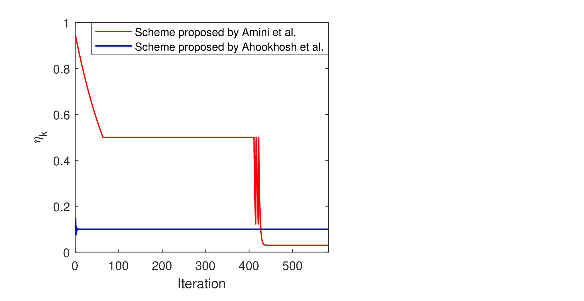
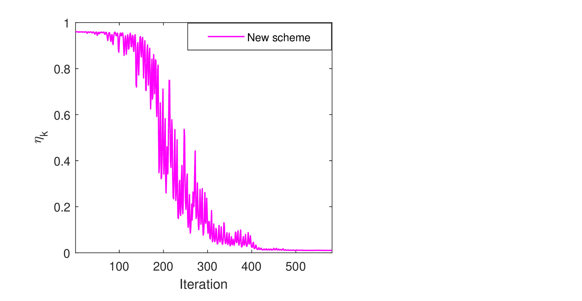
Figure 1: (Left): Values of $\eta_{k}$ proposed in (Ahookhosh et al., 2012) and (Amini et al., 2014), (Right): Values of $\eta_{k}$ for the new scheme.

As shown in Fig. 1, for the scheme proposed by Ahookhosh et al. (Ahookhosh et al., 2012), $\eta_{k}$ is close to $0.1$ after only a few iterations. Notice that $\eta_{k}$ in each iteration does not have any connection with the behaviour of the objective function. Thus this scheme is not effective. In addition, there are two issues with the scheme introduced by Amini et al. in (Amini et al., 2014). One problem indicated by Fig. 1 is that that $\eta_{k}$ decreases relatively quickly for the first 65 iterations. Since the algorithm requires the long iterations to solve his problem, ideally $\eta_{k}$ should be close to 1 for these initial iterations. The second problem is that the value of $\eta_{k}$ remains the same for a large number of iterations and it is not affected by the behaviour of the objective function.

To avoid theses challenges, we propose an adaptive strategy for calculating the value of $\eta_{k}$:

$$\eta_{k}=0.95\sin\left(\frac{\pi\|g_{k}\|}{1+2\|g_{k}\|}\right)+0.01.$$ (11)

When $x_{k}$ is far away from the minimizer, we can reasonably assume that $\|g_{k}\|$ is large. Thus the value of $\eta_{k}$ defined by (11) is close to 1. This makes the scheme closer to the original non-monotone strategy in the initial iterations, providing a chance to reduce the value of the objective function more significantly in the initial iterations. On the other hand, when $x_{k}$ is close to the minimizer, $\|g_{k}\|$ is small, then the value of $\eta_{k}$ is close to zero. Thus, the step length is small so that the new point stays in the neighbourhood of the optimal point. Thus the new scheme is closer to the monotone strategy. We plot the behaviour of $\eta_{k}$ denoted by (11) in Fig. 1 (Right), using the same values of the gradient for the optimization problem mentioned above.

2.2 New schemes for choosing $\alpha_{k}$

We utilize a convex combination of the Barzilai-Borwein (BB) step sizes to calculate an appropriate $\alpha_{k}$ in each outer iteration as in (Li and Wan, 2019). Our strategy calculates the value of $\alpha_{k}$, using the following equation:

$$\alpha_{k}^{{\scriptscriptstyle\textrm{CBB}}}=\mu_{k}\alpha^{(1)}_{k}+(1-\mu_{k})\alpha^{(2)}_{k},$$ (12)

where

$$\alpha_{k}^{(1)}=\frac{s_{k}^{T}s_{k}}{s_{k}^{T}y_{k}},\quad\alpha^{(2)}_{k}=\frac{s_{k}^{T}y_{k}}{y_{k}^{T}y_{k}},\quad s_{k}:=x_{k}-x_{k-1},\quad y_{k}:=g_{k}-g_{k-1};$$

$$\mu_{k}=\frac{K_{2}}{K_{1}+K_{2}}\quad K_{1}=\|\alpha^{(1)}_{k}y_{k}-s_{k}\|^{2},\quad K_{2}=\|(\alpha^{(2)}_{k})^{-1}s_{k}-y_{k}\|^{2}.$$

2.3 Conjugate gradient parameter

Here, we propose the new conjugate gradient parameter given by:

$$\beta_{k}=\omega\frac{\|g_{k}\|}{\|d_{k-1}\|},\quad\omega\in(0,1).$$ (13)

The complete algorithm is in Appendix 5 (see Algorithm 1). The next lemma proves a key property of $\beta_{k}$ which is very important in proving the algorithm’s convergence. The proofs are in the Appendix 5.

Lemma 2.1.

For the search direction $d_{k}$ and the constant $c>0$ we have:

$$d_{k}^{T}g_{k}\leq-c\|g_{k}\|.$$ (14)

The following assumptions are used to analyze the convergence properties of Algorithm 1.

H1

The level set $\mathcal{L}(x_{0})=\{x|f(x)\leq f(x_{0}),~{}~{}~{}~{}x\in\mathbb{R}^{n}\}$ is bounded set.

H2

The gradient of objective function is Lipschitz continuous over an open convex set $C$ containing $\mathcal{L}(x_{0})$. That is:

$$\|g(x)-g(y)\|\leq L\|x-y\|,\qquad\forall~{}x,y\in C.$$

We prove the following Theorem about the global convergence of Algorithm 1, the proof of which follows from the Lemmas presented in this section. Please see the appendix for the proofs.

Theorem 2.2.

Let $(H1)$, $(H2)$, and Lemmas 2.1 and 2.3 hold. Then, for the sequence $\{x_{k}\}$ generated by Algorithm 1, we have $\lim_{k\rightarrow\infty}\|g_{k}\|=0.$

Lemma 2.3.

Suppose that the search direction $d_{k}$ with the CG parameter $\beta_{k}$ given by (13) is generated by Algorithm 1. Then, an upper bound for $d_{k}$ is given by $\|d_{k}\|\leq(1+\omega)\|g_{k}\|.$

Lemma 2.4.

Suppose that $x_{k}$ is not a stationary point of (1). Then there exists a constant

$${\lambda}=\min\left\{\beta_{1}\rho,\frac{2(1-\omega)\rho(1-\gamma)}{L(1+\omega)^{2}}\right\},$$

such that $\alpha_{k}\geq{\lambda}$.

3 Numerical Results

In this section we test the new algorithm to solve a set of standard optimization problems and the non-negative matrix factorization problem, which is a non-convex optimization problem. The implementation level details are in Appendix 6. To demonstrate the efficiency of the proposed algorithm, we compare our algorithm and eight other existing algorithms introduced in (Ahookhosh et al., 2012; Amini et al., 2014; Jiang and Jian, 2019; Hager and Zhang, 2005) on a set of $110$ standards test problems. To describe the behaviour of each strategy, we use performance profiles proposed by Dolan and Moré (Dolan and Moré, 2002). Note that the performance profile for an algorithm $p_{s}(\tau):\mathbb{R}\mapsto[0,1]$ is a non-decreasing, piece-wise constant function, continuous from the right at each breakpoint. Moreover, the value $p_{s}(1)$ denotes the probability that the algorithm will win against the rest of the algorithm. More information on the performance profile is in Appendix 6. We plot the performance profile of each algorithm in terms of the total number of outer iteration and the CPU time on the set of standard test problems in Fig. 2.

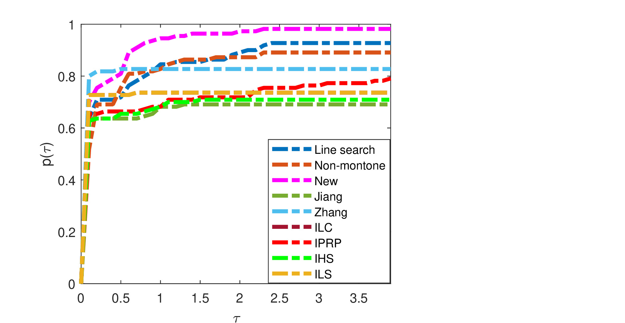
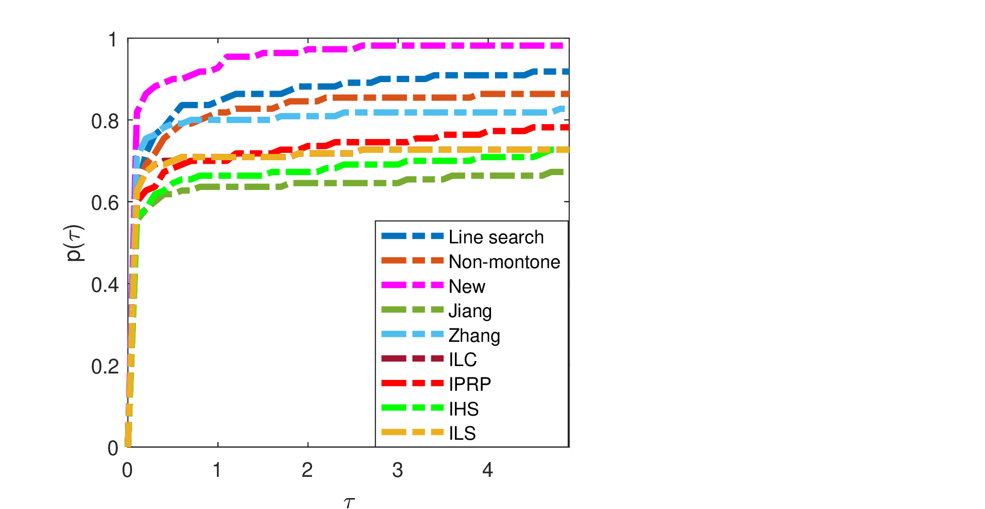
Figure 2: (Left): Performance profiles of the total number of outer iterations, (Right): Performance profiles of CPU Time.

We also apply our algorithm to solve the Non-Negative Matrix Factorization (NMF) which has several applications in image processing such as face detection problems. Given a non-negative matrix $V\in\mathbb{R}^{m\times n}$, a NMF finds two non-negative matrices $W\in\mathbb{R}^{m\times k}$ and $H\in\mathbb{R}^{k\times n}$ with $k\ll\min(m,n)$ such that $X\approx WH$. This problem can be formulated as

$$\min_{W,H\geq 0}F(W,H)=\frac{1}{2}\|V-WH\|_{F}^{2}.$$ (15)

Equation (15) is a non-convex optimization problem. We compare our method and Zhang’s algorithm (Hager and Zhang, 2005) on some random datasets and reported these results in Appendix 6.

4 Conclusion

In this paper, we introduced a new non-monotone conjugate gradient algorithm based on efficient Barzilai-Borwein step size. We introduced a new non-monotone parameter based on gradient behaviour and determined by a trigonometric function. We use a convex combination of the determined method to compute the step size value in each iteration. We prove that the proposed algorithm has global convergence. We implemented and tested our algorithm on a set of standard test problems and the non-negative matrix factorization problems. The proposed algorithm can solve $98\%$ of the test problems for a set of standard test instances. For the non-negative matrix factorization, the results indicate that our algorithm is more efficient compared to Zhang’ s method (Hager and Zhang, 2005).

5 Appendix A

5.1 Algorithm

In this section, we describe the new non-monotone conjugate gradient algorithm. Algorithm 1 consists of two loops, inner and outer loop. In each inner loop, the value of step size by using non-monotone line search strategy is computed and then the new point, search direction, and conjugate gradient parameter are calculated.

Input: $x_{0}\in\mathbb{R}^{n},~{}~{}\epsilon>0,~{}\rho\in(0,1),~{}~{}\gamma\in(0,1),$ and $N=5$

Output: $x^{*}$

Set: $k=0$

1 while $\|g_{k}\|\geq\epsilon$ do

2       while Eq. (7) is False do

3            $\alpha\leftarrow\rho\alpha$

4      $\alpha_{k}\leftarrow\alpha$

5       Generate the new point $x_{k+1}=x_{k}+\alpha_{k}d_{k}$

6       Compute the parameter $\beta_{k}$ by (13)

7       Generate $d_{k+1}$ by (5)

8       Calculate $\eta_{k+1}$ by using (11)

9       $k\leftarrow k+1$

Algorithm 1 An improved non-monotone conjugate gradient method

5.2 Convergence

The proofs of the various lemmas and the main theorem are presented in this section.

Proof.

Proof of Lemma 2.1:
If $k=0$, we have

$$d_{k}^{T}g_{k}=-\|g_{k}\|^{2}<0.$$

If $k\geq 1$, using (5) and (13), and we have:

$$d_{k}^{T}g_{k}=-\|g_{k}\|^{2}+\omega\frac{\|g_{k}\|}{\|d_{k-1}\|}d_{k-1}^{T}g_{k}.$$

Using the Cauchy-Schwarz inequality and we have:

$$d_{k}^{T}g_{k}\leq-\|g_{k}\|^{2}+\omega\|g_{k}\|^{2}=-(1-\omega)\|g_{k}\|^{2}.$$ (16)

∎

Proof.

Proof of Lemma 2.3:
The proof is obtained by combining (5) and the triangle inequality, that is:

$$\|d_{k}\|\leq\|g_{k}\|+\beta_{k}\|d_{k-1}\|=(1+\omega)\|g_{k}\|.$$

∎

To prove the convergence results, we need the following elementary lemmas.

Lemma 5.1.

Suppose that the sequence $\{x_{k}\}$ is generated by Algorithm 1. Then, $f_{l_{k}}$ is a decreasing sequence.

Proof.

We use the definition $R_{k}$ and (8), which imply that

$$R_{k}=\eta_{k}f_{l(k)}+(1-\eta_{k})f_{k}\leq\eta_{k}f_{l(k)}+(1-\eta_{k})f_{l(k)}=f_{l(k)}.$$ (17)

It follows that:

$$f_{k+1}\leq R_{k}+\gamma\alpha_{k}g_{k}^{T}d_{k}\leq f_{l(k)}+\gamma\alpha_{k}g_{k}^{T}d_{k}.$$

By using the Lemma 2.1, we can conclude that:

$$f_{k+1}\leq f_{l(k)}.$$ (18)

On the other hand, from (8) we have:

$$f_{l(k+1)} = \max_{0\leq j\leq m(k+1)}\left\{f_{k+1-j}\right\}$$

$$\leq \max_{0\leq j\leq m(k)+1}\left\{f_{k+1-j}\right\}=\max\left\{f_{l(k)},f_{k+1}\right\}.$$

By applying (18), that is $f_{k+1}\leq f_{l(k)}$, we conclude that $f_{l(k+1)}\leq f_{l(k)}$. This shows that the sequence $f_{l(k)}$ is a decreasing sequence. ∎

Lemma 5.2.

Suppose that the sequence $\{x_{k}\}$ is generated by Algorithm 1. Then, for all $k\geq{0}$, we have $x_{k}\in\mathcal{L}(x_{0})$.

Proof.

Definition of $f_{l(k+1)}$ implies that $f_{k+1}\leq f_{l(k+1)}$ for any $k\geq 0$. Therefore, we have:

$$f_{k+1} = \eta_{k+1}f_{k+1}+(1-\eta_{k+1})f_{k+1}$$ (19)

$$\leq \eta_{k+1}f_{l({k+1})}+(1-\eta_{k+1})f_{k+1}=R_{k+1},\qquad\forall~{}k\in N_{k}$$

By using definition of $R_{k}$, we can conclude that $R_{0}=f_{0}$. Now, by induction, assuming $x_{i}\in\mathcal{L}(x_{0})$, for all $i=1,2,\ldots,k$, we show that $x_{k+1}\in\mathcal{L}(x_{0})$. Relations (8) and (17) together with Lemma 5.1 imply that:

$$f_{k+1}\leq f_{l(k+1)}\leq f_{l(k)}\leq f_{0},$$

which implies that the sequence ${x_{k}}$ is contained in $\mathcal{L}(x_{0})$. ∎

The next part of this section describes some convergence results for the Algorithm 1.

Lemma 5.3.

Suppose that Algorithm 1 generates the sequence $\{x_{k}\}$ and ($H1$)–($H2$) hold. Then, the sequence $\{f_{l(k)}\}$ is convergent.

Proof.

By using Lemma 5.1 and the fact that $f_{l(0)}=f_{0}$ imply that the sequence $\{x_{l(k)}\}$ remains in level set $\mathcal{L}(x_{0})$. On the other hand, this fact $f(x_{k})\leq f(x_{l(k)})$ proves that the sequence $\{x_{k}\}$ remains in $\mathcal{L}(x_{0})$. Therefore, ($H1$) together with Lemma 5.1 imply that the sequence $\{f_{l(k)}\}$ is convergent. ∎

Lemma 5.4.

Suppose that (H1) holds and the direction $d_{k}$ satisfies the first item of Lemma 5.1. Then for the sequence $\{x_{k}\}$ generated by Algorithm 1, we have:

$$\lim_{k\rightarrow\infty}f_{l(k)}=\lim_{k\rightarrow\infty}f_{k}.$$

Proof.

The proof is similar to Lemma 2 in [Amini et al., 2014]. Therefore, we omit it here. ∎

Lemma 5.5.

Suppose that (H1) holds and the direction $d_{k}$ satisfies the first item of Lemma 5.1. If the sequence $\{x_{k}\}$ generated by Algorithm 1, then we have:

$$\lim_{k\rightarrow\infty}R_{k}=\lim_{k\rightarrow\infty}f_{k}.$$

Proof.

Using (17) and (19), we conclude that:

$$f_{k}\leq R_{k}\leq f_{l(k)}$$

By applying Lemma 5.4, we obtain the result. ∎

Now, we can prove the Lemma 2.4.

Proof.

Proof of Lemma 2.4:
We consider two cases: If $\frac{\alpha_{k}}{\rho}\geq\beta_{1}$, which implies that $\alpha_{k}\geq\beta_{1}\rho$ and it completes the proof. Now, we assume that $\frac{\alpha_{k}}{\rho}<\beta_{1}$. In this case we have $\alpha_{k}<\beta_{1}\rho$. Therefore, the non-monotone condition does not hold, i.e.,

$$f(x_{k}+\frac{\alpha_{k}}{\rho}d_{k})>R_{k}+\gamma\frac{\alpha_{k}}{\rho}g_{k}^{T}d_{k}$$ (20)

Now, by using the mean value theorem, i.e., Cauchy–Schwarz inequality, we conclude that:

$$f(x_{k}+\alpha d_{k}) = f(x_{k})+\alpha g_{k}^{T}d_{k}+\int_{0}^{1}\alpha(g(x_{k}+t\alpha d_{k})-g_{k})^{T}d_{k}dt$$

$$\leq f(x_{k})+\alpha g_{k}^{T}d_{k}+\alpha\|d_{k}\|\int_{0}^{1}\|(g(x_{k}+t\alpha d_{k})-g_{k}^{T})\|dt$$

Now, by using ($H2$) and the fact that $R_{k}\geq f_{k}$, we have:

$$f(x_{k}+\alpha d_{k}) \leq f(x_{k})+\alpha g_{k}^{T}d_{k}+L\alpha^{2}\|d_{k}\|^{2}\int_{0}^{1}tdt$$ (22)

$$= f(x_{k})+\alpha g_{k}^{T}d_{k}+\frac{L}{2}\alpha^{2}\|d_{k}\|^{2}$$

$$\leq R_{k}+\alpha g_{k}^{T}d_{k}+\frac{L}{2}\alpha^{2}\|d_{k}\|^{2}$$

By putting $\alpha=\frac{\alpha_{k}}{\rho}$ and combining (20) with (22), we conclude that:

$$R_{k}+\frac{\alpha_{k}}{\rho}g_{k}^{T}d_{k}+\frac{L}{2\rho^{2}}\alpha_{2}^{2}\|d_{k}\|^{2}\geq R_{k}+\gamma\frac{\alpha_{k}}{\rho}g_{k}^{T}d_{k}.$$

Using Lemmas 2.1 and 2.3, we conclude that:

$$\frac{L}{2\rho}(1+\omega)^{2}\alpha_{2}^{2}\|g_{k}\|^{2}\geq\frac{L}{2\rho}\alpha_{2}^{2}\|d_{k}\|^{2}>-(1-\gamma)g^{T}_{k}d_{k}\geq(1-\omega)(1-\gamma)\|g_{k}\|^{2}.$$ (23)

It implies that:

$$\alpha_{k}\geq\frac{2(1-\omega)\rho(1-\gamma)}{L(1+\omega)^{2}}.$$

∎

Now, we prove the Theorem 2.2, which shows that Algorithm 1 has global convergence.

Proof.

Proof of Theorem 2.2:
We have:

$$R_{k}+\gamma\alpha_{k}g^{T}_{k}d_{k} \geq f_{k+1}$$

$$\Rightarrow R_{k}-f_{k+1} \geq -\gamma\alpha_{k}g^{T}_{k}d_{k}\geq c_{1}\gamma\alpha_{k}\|g_{k}\|^{2}\geq 0.$$ (24)

This fact together with Lemma 5.5 imply that $\lim_{k\rightarrow\infty}\|g_{k}\|=0$. This shows that proposed algorithm has global convergence. ∎

6 Appendix B

6.1 Numerical Results

Here, we present some implementation level details. Since our algorithm improves the non-monotone scheme, we chose two algorithms from the non-monotone line search category and six algorithms from the Wolfe line search area for performing the comparison. We select the following two state of art algorithms in the non-monotone category. These algorithms calculate the value of step size using a the non-monotone line search strategy in each iteration.

$\bullet$

Ahookhosh’s strategy in [Ahookhosh et al., 2012]

$\bullet$

Amini’s strategy in [Amini et al., 2014]

Following six other algorithms that use the Wolfe line search conditions to compute step size in each iteration are used for comparison.

$\bullet$

$\beta^{Jiang}$ proposed in [Jiang and Jian, 2019]

$\bullet$

$\beta^{Zhang}$ proposed in [Hager and Zhang, 2005]

$\bullet$

$\beta^{ILC}$ proposed in [Jiang and Jian, 2019]

$\bullet$

$\beta^{IPRP}$ proposed in [Jiang and Jian, 2019]

$\bullet$

$\beta^{IHS}$ proposed in [Jiang and Jian, 2019]

$\bullet$

$\beta^{ILS}$ proposed in [Jiang and Jian, 2019]

All algorithms were coded in MATLAB 2017 environment and tested on a laptop (Intel(R) Core(TM) i5-7200U CPU 3.18 GHz with 12GB RAM). For all algorithms, we use the following initial values.

$$\gamma=10^{-4},\qquad N=5,\qquad\rho=0.75,\qquad c=10^{-4}.$$

All the experiments terminate when the following conditions are met:

$\bullet$

$\|g_{k}\|<10^{-6}$

$\bullet$

The number of iterations is greater than 20000.

As parameter $\omega$ can take positive real values in the interval $(0,1)$, there are many choices for it. We tried several strategies and chosen the following strategy, which perform better. The key idea of this choice is from the structure of the conjugate gradient parameter proposed by Jiang [Jiang and Jian, 2019].

$$\omega_{k}=\left\{\begin{array}[]{lr}0.001\qquad\qquad\quad\qquad if~{}\frac{|g^{T}_{k}d_{k-1}|}{-g^{T}_{k-1}d_{k-1}}\leq 0,&\\ 0.999\qquad\qquad\quad\qquad if~{}\frac{|g^{T}_{k}d_{k-1}|}{-g^{T}_{k-1}d_{k-1}}\geq 1,&\\ \frac{|g^{T}_{k}d_{k-1}|}{-g^{T}_{k-1}d_{k-1}}\qquad\qquad\qquad otherwise.&\\ \end{array}\right.$$

The following subsection presents the results on a set of $110$ standard test problems.

6.2 A set of standard test problems

We run all the algorithms on 110 standard test problems from [Andrei, 2008] with dimensions ranging between $2$ to $5,000,000$. When the algorithm stops under the second condition, i.e., the number of iterations is greater than $20000$, the method is deemed to fail for solving the corresponding test problem. The comparison between considered algorithms is based on the number of function evaluations, the number of gradient evaluations, the number of iterations, and the CPU time(s).
To visualize the complete behaviour of the algorithms, we use the performance profiles proposed by Dolan and Moré [Dolan and Moré, 2002]. Note that the performance profile $p_{s}(\tau):\mathbb{R}\mapsto[0,1]$ for an algorithm is a non-decreasing, piece-wise constant function, continuous from the right at each breakpoint. Moreover, the value of $p_{s}(1)$ denotes the probability that the algorithm will win over the rest.

Suppose that $K$ is a set of $n_{k}$ test functions and $S$ is a set of $n_{s}$ solvers. For $s\in S$ and function $k\in K$, consider $a_{p,s}$ as the number of gradient evaluations, objective function evaluations, CPU Time, or the number of iterations required to solve function $k\in K$ by algorithm $s\in S$. Then the algorithms comparison is based on the performance ratio as follows:

$$r_{k,s}=\frac{a_{k,s}}{\min\{a_{k,s},~{}k\in K,~{}s\in S\}}$$

We obtain the overall evaluation of each algorithm by:

$$p_{s}(\tau)=\frac{1}{n_{k}}~{}size~{}\{k\in K:r_{k,s}\leq\tau\}$$ (26)

In general, solvers with high values of $p_{s}(\tau)$ or in the upper right of the figure represent the best algorithm.

The performance profile in terms of function evaluations and the number of gradient evaluations are presented in figures 3 and 4, respectively.

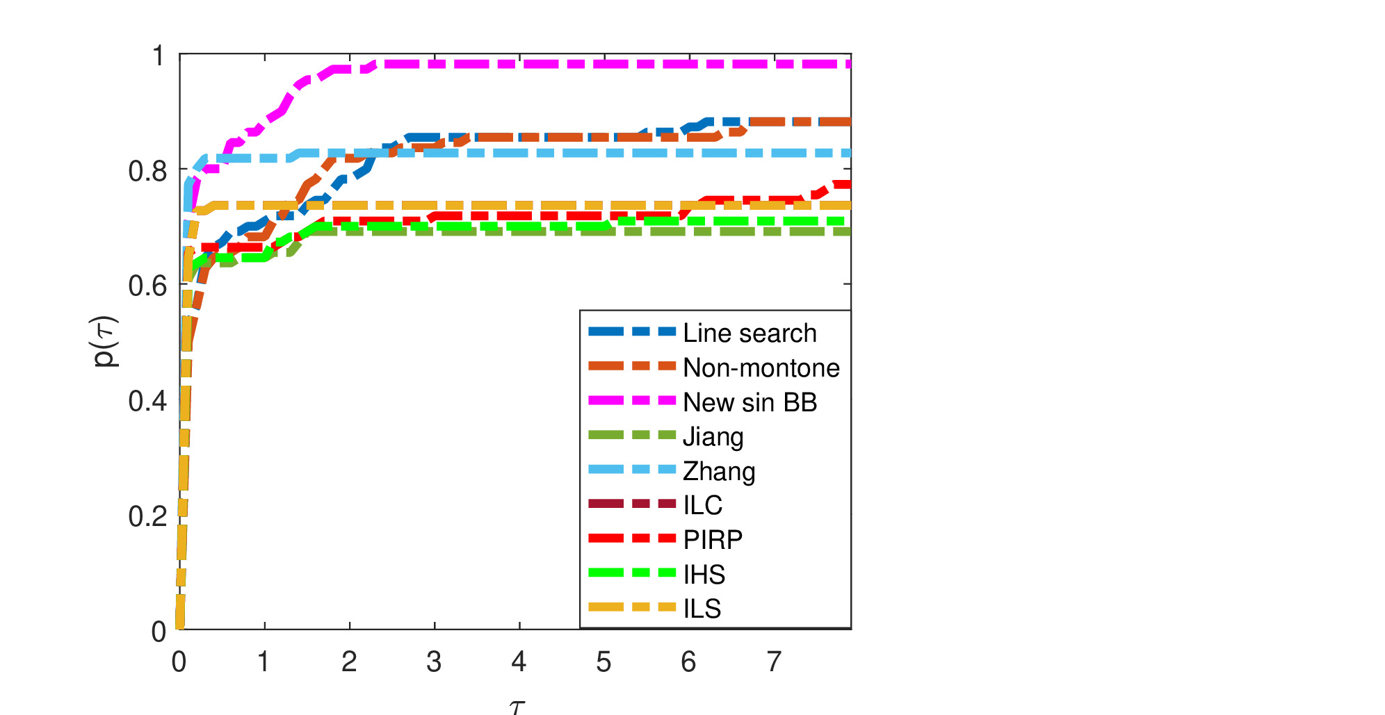
Figure 3: Performance profiles of the total number of function evaluations

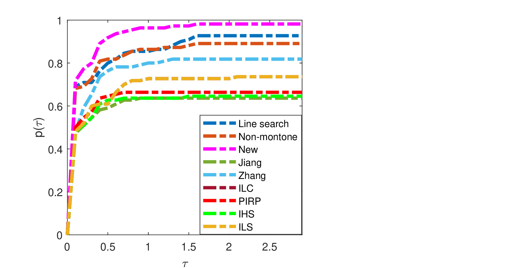
Figure 4: Performance profiles of the total number of gradient evaluations

Figures 5 and 6 show the performance profile in terms of the number of iterations and the CPU time(s) for the proposed algorithm and eight other algorithms.

Figure 5: Performance profiles of the total number of outer iterations

Figure 6: Performance profiles of CPU Time

We conclude from the figures that the proposed algorithm can solve $98\%$ of the test problems. The performance profiles for the number of iterations, total CPU, time, number of gradient evaluations, and number of function evaluations indicate that the proposed method has a high computational performance compared to the other methods.

6.3 Some non-negative matrix factorization test problems

Here, we apply our algorithm to Non-Negative Matrix Factorization (NMF) which has several applications in image processing, such as face detection problems. Given a non-negative matrix $V\in\mathbb{R}^{m\times n}$, a NMF finds two non-negative matrices $W\in\mathbb{R}^{m\times k}$ and $H\in\mathbb{R}^{k\times n}$ with $k\ll\min(m,n)$ such that

$$V\approx WH.$$ (27)

This problem can be formulated as a non-convex optimization problem:

$$\min_{W,H\geq 0}F(W,H)=\frac{1}{2}\|V-WH\|_{F}^{2}.$$ (28)

In recent years, several iterative approaches have been introduced for solving (28), for example, [Han et al., 2009, Lee and Seung, ]. The alternating non-negative least squares (ANLS) framework is a popular approach for solving (28), which finds the optimal solution by solving the following two convex sub-problems:

$$W^{k+1}=\text{arg}\min_{W\geq 0}F(W,H^{k})=\frac{1}{2}\|V-WH^{k}\|_{F}^{2},$$ (29)

and

$$H^{k+1}=\text{arg}\min_{H\geq 0}F(W^{k+1},H)=\frac{1}{2}\|V-W^{k+1}H\|_{F}^{2}.$$ (30)

To solve this problem, we use the following strategy:

S0

Algorithm starts with the initial point, i.e., $\bar{W}\geq 0$ and $\bar{H}\geq 0$, set $k=0$.

S1

Stop if $\|[\nabla_{H}F(\bar{W}^{k},\bar{H}^{k}),\nabla_{W}F(\bar{W^{k}},\bar{H}^{k})]\|_{F}\leq\epsilon\|[\nabla_{H}F(\bar{W^{0}},\bar{H^{0}}),\nabla_{W}F(\bar{W^{0}},\bar{H}^{0})]\|_{F}.$

S2

To get $W^{k+1}$, solve the sub-problem: $\min_{W\geq 0}F(W,\bar{H}^{k})=\frac{1}{2}\|V-W\bar{H}^{k}\|_{F}^{2}$.

S4

Set $\bar{W}^{k+1}=W^{k+1}$.

S2

To get $H^{k+1}$, solve the sub-problem: $\min_{H\geq 0}F(\bar{W}^{k+1},H)=\frac{1}{2}\|V-\bar{W}^{k+1}H\|_{F}^{2}$.

S5

Set $\bar{H}^{k+1}=H^{k+1}$.

S6

Set $k:=k+1$ and go to S1.

Now, we use the above setup to solve some NMF problems using our algorithm and compare it to Zhang’s algorithm [Hager and Zhang, 2005] which had the best results for solving a set of standard test problems. To this end, we generate a random matrix $V$ as random with elements in $[0,1]$. We run the algorithm for matrices with ranks $\{5,10,15,20,40,50\}$. For each case, we run each of the algorithms 10 times. We, calculated the average of the results and presented them in Table 1. In this table, $m$ and $n$ denote the number of rows and columns of matrix $V$, $k$ denote the matrix rank. The number of outer iterations is denoted by “Iter”. We use the “Niter” for the number of inner iterations. The value of gradient is denoted by “Pgn”. The CPU time and error for each of the algorithms are denoted by “Time” and “Error” respectively.

$m$        $n$        $k$	${Iter}$	${Niter}$	${Pgn}$	${Time}$	$Error$	$Algorithm$
$50\times 25\times 5$	29.20	187.30	0.0045	0.02	0.014	Zhang
	26.70	72.60	0.0043	0.02	0.014	New
$100\times 50\times 5$	24.20	165.30	0.058	0.03	0.12	Zhang
	22.30	85.80	0.033	0.01	0.12	New
$100\times 200\times 15$	25.30	196.10	0.015	0.137	0.086	Zhang
	17.50	112.80	0.018	0.032	0.085	New
$200\times 100\times 10$	19.00	134.80	.093	0.10	0.08	Zhang
	17.10	103.40	.073	0.03	0.08	New
$300\times 100\times 20$	25.00	212.40	0.55	0.32	0.08	Zhang
	20.60	131.50	0.44	0.15	0.08	New
$300\times 500\times 20$	29.00	128.90	1.98	0.75	0.054	Zhang
	25.80	90.80	0.96	0.14	0.054	New
$500\times 100\times 20$	36.10	231.80	7.6	0.48	0.06	Zhang
	31.70	90.70	4.8	0.12	0.05	New
$1000\times 500\times 50$	36.10	187.50	18.5	2.89	0.04	Zhang
	32.40	130.80	12.75	1.06	0.03	New

Table 1: The results of performing new algorithm and Zhang’s algorithm on some random datasets

As we see that in most cases, the proposed algorithm performs better than previous best algorithm due to Zhang [Hager and Zhang, 2005].

References

- Barzilai and Borwein [1988] Jonathan Barzilai and Jonathan M Borwein. Two-point step size gradient methods. IMA journal of numerical analysis, 8(1):141–148, 1988.
- Nocedal and Wright [2006] Jorge Nocedal and Stephen Wright. Numerical optimization. Springer Science & Business Media, 2006.
- Hestenes et al. [1952] Magnus Rudolph Hestenes, Eduard Stiefel, et al. Methods of conjugate gradients for solving linear systems, volume 49. NBS Washington, DC, 1952.
- Fletcher and Reeves [1964] Reeves Fletcher and Colin M Reeves. Function minimization by conjugate gradients. The computer journal, 7(2):149–154, 1964.
- Fletcher [2013] Roger Fletcher. Practical methods of optimization. John Wiley & Sons, 2013.
- Polak and Ribiere [1969] Elijah Polak and Gerard Ribiere. Note sur la convergence de méthodes de directions conjuguées. ESAIM: Mathematical Modelling and Numerical Analysis-Modélisation Mathématique et Analyse Numérique, 3(R1):35–43, 1969.
- Grippo et al. [1986] Luigi Grippo, Francesco Lampariello, and Stephano Lucidi. A nonmonotone line search technique for newton’s method. SIAM journal on Numerical Analysis, 23(4):707–716, 1986.
- Zhang and Hager [2004] Hongchao Zhang and William W Hager. A nonmonotone line search technique and its application to unconstrained optimization. SIAM journal on Optimization, 14(4):1043–1056, 2004.
- Ahookhosh et al. [2012] Masoud Ahookhosh, Keyvan Amini, and Mohammad Reza Peyghami. A nonmonotone trust-region line search method for large-scale unconstrained optimization. Applied Mathematical Modelling, 36(1):478–487, 2012.
- Li and Wan [2019] Ting Li and Zhong Wan. New adaptive barzilai–borwein step size and its application in solving large-scale optimization problems. The ANZIAM Journal, 61(1):76–98, 2019.
- Nazareth [1999] JL Nazareth. Conjugate-gradient methods, encyclopedia of optimization, c. floudas and p. pardalos, eds, 1999.
- Esmaeili and Kimiaei [2014] Hamid Esmaeili and Morteza Kimiaei. A new adaptive trust-region method for system of nonlinear equations. Applied mathematical modelling, 38(11-12):3003–3015, 2014.
- Ahookhosh and Amini [2012] Masoud Ahookhosh and Keyvan Amini. An efficient nonmonotone trust-region method for unconstrained optimization. Numerical Algorithms, 59(4):523–540, 2012.
- Amini and Ahookhosh [2014] Keyvan Amini and Masoud Ahookhosh. A hybrid of adjustable trust-region and nonmonotone algorithms for unconstrained optimization. Applied Mathematical Modelling, 38(9-10):2601–2612, 2014.
- Ahookhosh and Ghaderi [2017] Masoud Ahookhosh and Susan Ghaderi. On efficiency of nonmonotone armijo-type line searches. Applied Mathematical Modelling, 43:170–190, 2017.
- Amini et al. [2014] Keyvan Amini, Masoud Ahookhosh, and Hadi Nosratipour. An inexact line search approach using modified nonmonotone strategy for unconstrained optimization. Numerical Algorithms, 66(1):49–78, 2014.
- Jiang and Jian [2019] Xianzhen Jiang and Jinbao Jian. Improved fletcher–reeves and dai–yuan conjugate gradient methods with the strong wolfe line search. Journal of Computational and Applied Mathematics, 348:525–534, 2019.
- Hager and Zhang [2005] William W Hager and Hongchao Zhang. A new conjugate gradient method with guaranteed descent and an efficient line search. SIAM Journal on optimization, 16(1):170–192, 2005.
- Dolan and Moré [2002] Elizabeth D Dolan and Jorge J Moré. Benchmarking optimization software with performance profiles. Mathematical programming, 91(2):201–213, 2002.
- Andrei [2008] Neculai Andrei. An unconstrained optimization test functions collection. Adv. Model. Optim, 10(1):147–161, 2008.
- Han et al. [2009] Lixing Han, Michael Neumann, and Upendra Prasad. Alternating projected barzilai-borwein methods for nonnegative matrix factorization. Electron. Trans. Numer. Anal, 36(6):54–82, 2009.
- [22] DD Lee and HS Seung. Algorithms for non-negative matrix factorization. nips (2000). Google Scholar, pages 556–562.