Physical limits on electromagnetic response

Abstract

Photonic devices play an increasingly important role in advancing physics and engineering, and while improvements in nanofabrication and computational methods have driven dramatic progress in expanding the range of achievable optical characteristics, they have also greatly increased design complexity. These developments have led to heightened relevance for the study of fundamental limits on optical response. Here, we review recent progress in our understanding of these limits with special focus on an emerging theoretical framework that combines computational optimization with conservation laws to yield physical limits capturing all relevant wave effects. Results pertaining to canonical electromagnetic problems such as thermal emission, scattering cross sections, Purcell enhancement, and power routing are presented. Finally, we identify areas for additional research, including conceptual extensions and efficient numerical schemes for handling large-scale problems.

Photonics has become an indispensable tool of scientific discovery, enabling key advances in communications [1], sensing [2, 3], photovoltaics [4], computing [5, 6], quantum engineering [7, 8], and many other fields. At the center of the broad applicability of optical methods is a small but powerful set of design schemes for confining and transferring energy in time and space—notions such as index guiding, wave interference, polaritonics, and effective medium engineering—that provides physical intuition for extracting concrete functionality from the abstract mathematical richness within Maxwell’s equations. Each offers a mixture of distinctive capabilities and limitations, and determining the best approach or combination of approaches for any particular application remains a subject of continuing challenge for photonics design [9].

As a concrete example, consider the problem of enhancing light-matter interactions via the photonic local density of states (LDOS)—the Purcell effect—reducing to the familiar Purcell factor $F_{P}=\frac{6}{\pi^{2}}\left(\frac{\lambda}{2n}\right)^{3}\frac{Q}{V}$ in the case where a single resonance dominates [10]. Integrated micro-resonators [11] based on index guiding can achieve extremely long lifetimes (high quality factors $Q$) at the expense of reduced spatial localization (large mode volumes $V$). Electronic plasmon- and phonon-polariton resonances allow for tight subwavelength confinement (small $V$) but suffer from high material absorption (small $Q$) [12]. Photonic crystals [10] and bandgap engineering provide a flexible low-loss platform for manipulating light at the wavelength scale but are limited in practice by achievable bandwidths and a lack of forms exhibiting omnidirectional bandgaps. Metamaterials offer conceptual simplicity in engineering exotic dispersions and large LDOS [13] but in practice are constrained by fabrication limitations, the breakdown of effective-medium approximations at large wavenumbers, and challenges related to light coupling [14, 15].

Growing out of these general design principles, continued increases in computational power have paved the way for the development of inverse methods that, given a set of desired electromagnetic objectives and constraints, exploit global [16], gradient-based [17, 18, 19], and data-driven optimization algorithms [20, 21] to search through potentially millions of structural degrees of freedom in pursuit of ideal response characteristics. This capacity has greatly expanded the accessible design space, and has led to vast improvements in device performance. However, for typical problems, the vast range of design possibilities and complicated interplay between standard objectives and constraints also makes it practically impossible to determine truly optimal structures, and one can at most hope for a well performing local optimum . While our arsenal of design techniques and algorithms gives us enormous capability to tackle a wide range of engineering applications, it cannot rigorously answer a natural question of increasing relevance: what are the fundamental limits to optical control and how close are existing devices to reaching them?

The notion of fundamental limits, encoded in bedrock principles like the finite speed of light and second law of thermodynamics, is ubiquitous in physics. Beyond added theoretical understanding, limits have and continue to play an important role as signposts for further technological improvement. Attempts to overcome the Abbe diffraction limit led in large part to the development of the field of super-resolution microscopy, with diverse techniques exploiting evanescent fields [23, 24, 25], nonlinear effects [24, 26], and active temporal control [27]. Knowledge of the physical origins of the factors forming the Shockley-Queisser limit [28] for solar cell efficiency pointed the way to diverse developments in concentrators [29], tandem [30], and intermediate band photovoltaics [31]. The breakdown of familiar blackbody limits to nanoscale separations sparked interest in super-Planckian thermal devices [32, 33].

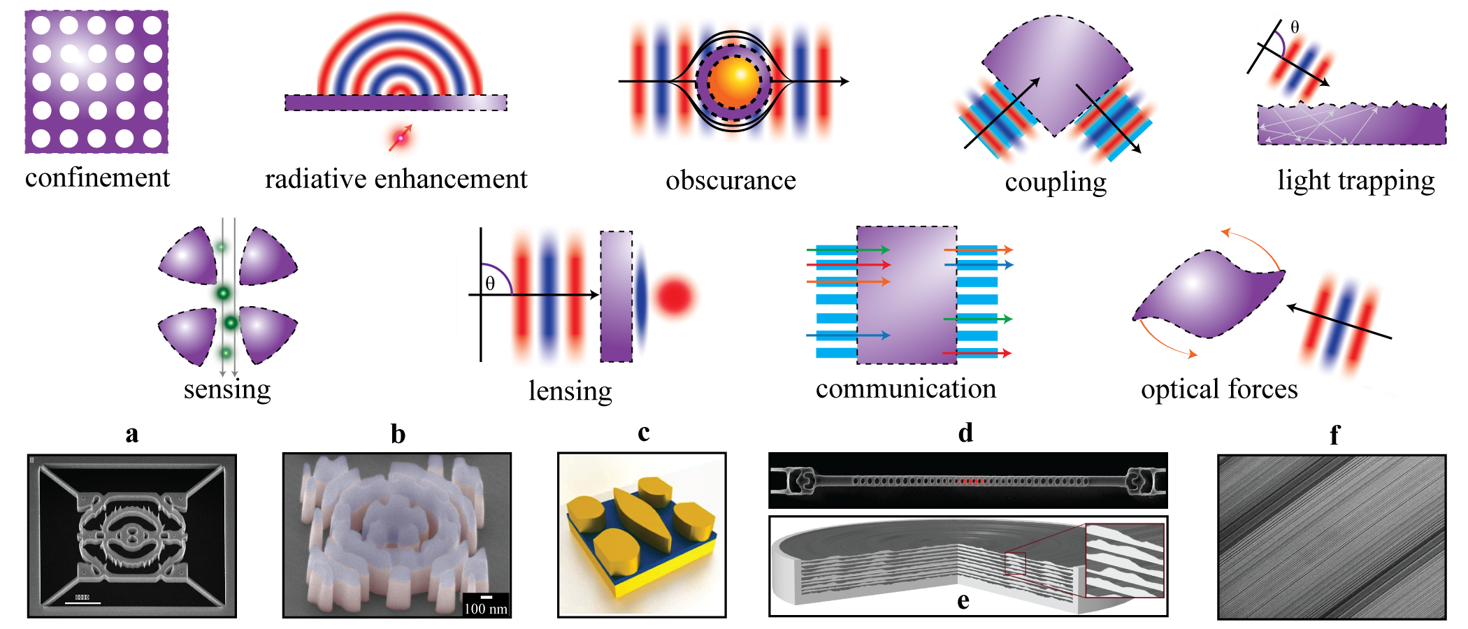
Figure 1: Applications of photonics and computational design. The top part of the figure shows a collection of representative photonic functionalities. In each instance, performance is critically effected by the possibility of using (sub)wavelength-scale structuring to confine or transform optical fields and, as such, is intrinsically linked to physical limits on these phenomena. The bottom part of the figure depicts several (recent) examples of computationally synthesized devices for achieving improved performance in the operations shown above. Moving from left to right, these examples are a a dielectric cavity achieving nanometer scale confinement, Ref. [34]; b a “photon extractor” enhancing the emission collection rate of a nitrogen vacancy center, Ref. [8]; c a frequency selective emitter for thermo-photovoltaic applications, Ref. [35]; d a photon-extractor (i.e. cavity and coupler) for diamond photonics, Ref. [7]; e and f large area, high-efficiency, metalenses, Ref. [36] and Ref. [37] respectively.

In this review, we first present a historical overview on the development of electromagnetic limits, following representative examples that illustrate a general thematic evolution essentially mirroring the history of optics itself: from simplifying and restrictive assumptions (homogeneity, quasistatics, and ray optics, etc.) pertinent to low-dimensional, deeply subwavelength, and large-etalon systems, toward increasingly sophisticated wave arguments applicable to any length scale. We then focus our discussion on an emerging general methodology for evaluating photonic design bounds based on optimization theory and conservation principles that follow either directly from Maxwell’s equations or the identities of scattering theory. Originally developed as an instrument for investigating maximal scattering cross section limits [38, 39, 40], the framework is applicable to a broad range of design problems where the objective can be expressed as a quadratic function of the fields [41, 42, 43]. The constraints have clear physical meaning, limiting both the amplitude of the polarization response, important to power transfer, and the extent that the phase of the polarization response can be modified, with consequences on the engineering of resonances. To better handle problems involving near field effects and rapidly varying length scales, spatially localized constraints can be introduced, with a denser distribution of local constraints giving tighter bounds at the expense of higher computational complexity [41, 42]. In this sense the framework emphasizes the complementary role of limits and structural optimization: structural optimization enforces Maxwell’s equations exactly (up to computational discretization) and produces specific devices corresponding to local optima; the limits framework instead produces bounds that apply to all possible structures via conservation-law based constraints over spatial regions that can be viewed as a relaxation of Maxwell’s equations.

Through instructive results concerning thermal emission, scattering/absorption cross sections, LDOS enhancement, and power splitting, we describe physical implications behind various components of the framework, drawing connections to well-known prior results and demonstrating its broad applicability. For readers interested in the mathematical details of the underlying optimization theory, we also recommend the excellent review by Angeris et al. Ref. [44]. Finally, we detail remaining challenges and opportunities, including the need for numerical methods that can handle larger systems, generalizations to other physical settings beyond photonics, and potential improvements to structural optimizations that may arise from knowledge of optimal fields.

Historical overview

Since the first measurement of the speed of light in vacuum by Rømer, and the subsequent postulates of special relativity demanding that information cannot travel faster than $c$, rigorous proofs of subluminal energy velocity $v_{e}\leq c$ have been deduced from increasingly general assumptions, moving from homogeneous non-absorbing media, through the inclusion of dispersion, anisotropy, and nonlocality [45, 46, 47, 48], to the simple unifying requirement of passivity: materials which do no net work on electromagnetic fields [49, 48, 50]. In complement, there has also been great interest in establishing limits on minimal energy velocity or “slow light”, i.e., engineered devices such as optical delay lines and buffers [51, 52, 53, 54, 55]. Under the approximation of zero bandwidth, the delay experienced by a light pulse can essentially be made indefinitely long, e.g., near the band edge of a photonic crystal where the group velocity vanishes [56]. For finite bandwidths, however, delay-bandwidth product limits (e.g., the uncertainty principle) must set a fundamental lower bound. For a slow light waveguide with an idealized linear dispersion relation across the bandwidth of interest, the delay bandwidth product limit takes the form $\Delta T\Delta f\leq\frac{L}{\lambda_{c}}(n_{avg}-n_{min})$, where L is the length of the device, $\lambda_{c}$ is the free-space bandwidth at the band center, and $n_{avg}$, $n_{min}$ are the average and minimum effective index of refraction across the bandwidth, respectively [51]. For the simple case of explicitly 1D wave propagation and material structuring, more general bounds can be derived without the notion of an effective index of refraction and the assumption of idealized linear dispersion: $\Delta T\Delta f\leq\frac{1}{2\sqrt{3}}\frac{L}{\lambda_{c}}\frac{\max\lVert\epsilon(z,f)-\epsilon_{ro}\rVert}{\epsilon_{ro}}$, where $\epsilon(z,f)$ is the (possibly complex) relative dielectric constant as a function of the propagation coordinate $z$ and frequency $f$, $\epsilon_{ro}$ is the relative dielectric constant of the background medium, and the maximum is taken across space and bandwidth [57, 58]. Further work is needed to extend these results to accommodate rigorous full-wave descriptions of three-dimensional structures.

Related bandwidth arguments have also been used to derive performance bounds on optical cloaks—devices that eliminate or greatly reduce scattering of incident light [59]. Most commonly, metamaterial cloaks are designed via transformation optics to carry out prescribed phase and amplitude manipulations by mapping coordinate transformations, $\mathbf{x}\to\mathcal{J}\mathbf{x}^{\prime}$, onto effective homogenized susceptibility parameters, $\{\epsilon,\mu\}\to\{\epsilon^{\prime},\mu^{\prime}\}=\frac{\mathcal{J}^{\dagger}\{\epsilon,\mu\}\mathcal{J}}{\mathrm{det}\mathcal{J}}$, in a design volume surrounding the object. Because light must go around the cloaked object and maintain an unperturbed wavefront, the phase velocity in any cloak must be superluminal, necessitating the existence of dispersion in order to respect causality, and thereby precluding perfect cloaking in vacuum over any finite bandwidth [60]. One way around this limitation is to consider “ground-plane” cloaking, wherein the object to be concealed is positioned adjacent to a reflecting boundary. With this shift in perspective, the original causality constraint does not apply, as the reflected waves from the cloak travel a shorter distance than reflected waves from the ground plane itself. Yet, because the wavefront within the cloak must now be delayed, the basic challenge posed by the need to respect delay-bandwidth limits remains, and, in the simplifying case of 1D waves, leads to a bound on the minimum thickness of the cloak $d\gtrsim\frac{h}{n(n-1)}\frac{\Delta\omega}{\omega}$ as a function of the object size $h$ and the bandwidth $\Delta\omega$. Generalizing to 3D [61], any ground plane cloak must obey the inequality $V_{c}\geq V_{c}^{\prime}/B$ where $V_{c}$ is the volume of the cloak, $V_{c}^{\prime}$ is combined volume of cloak and object, $B$ represents the maximum achievable index contrast (eigenvalues of $\mathcal{J}^{T}\mathcal{J}$). While instructive, determining attainable $\mathcal{J}$, and hence $B$, requires specific geometric analyses.

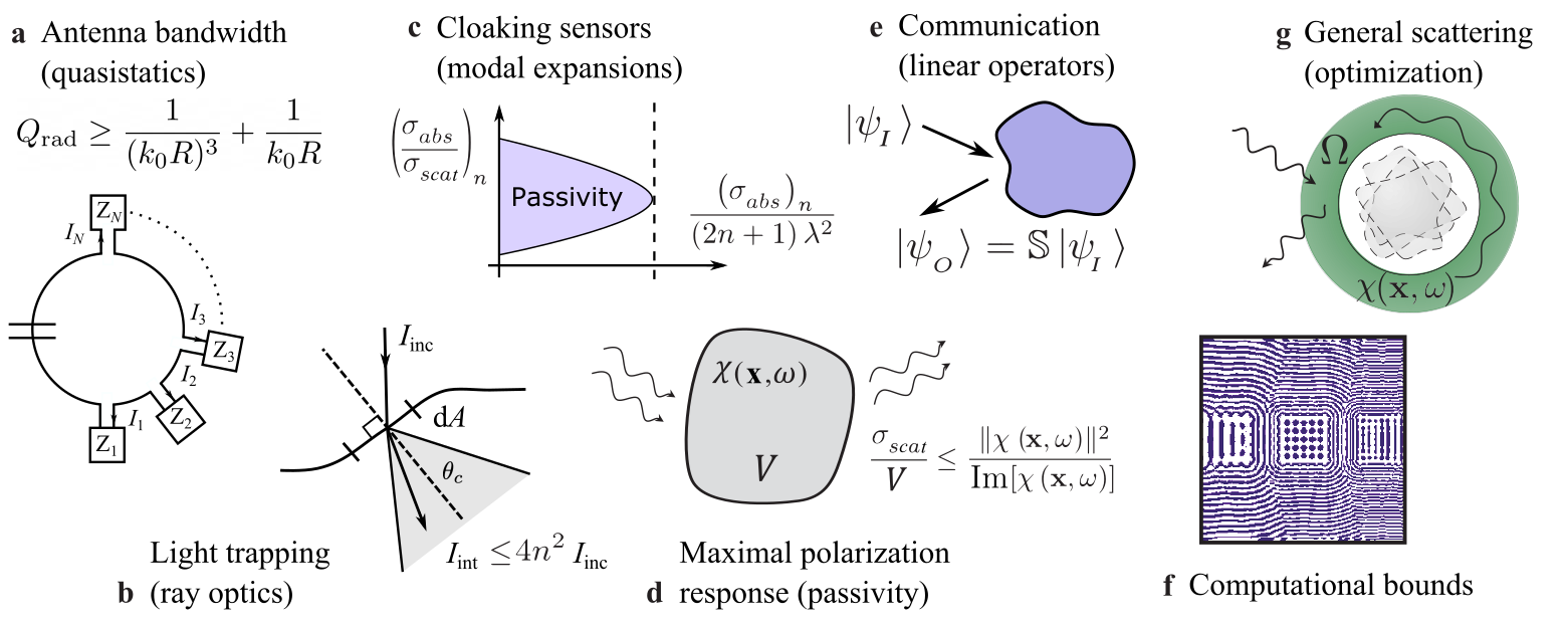
Figure 2: Overview of representative electromagnetic limits. The figure illustrates a collection of representative photonic bounds, arranged from left to right in roughly chronological order. a Equivalent circuit of an omnidirectional antenna, adapted from [62]. For electrically small antennas, taking the quasistatic limit yields the celebrated Chu limit. b Yablonovitch limits to light trapping at a rough interface, combining geometric (ray) optics with a statistical description of the scattering angle [63]. c and d Limits based on passivity: for a passive device both the absorbed and scattered power must be non-negative. c shows the feasible region for cloaking as a function of absorption efficiency $\sigma_{sca}/\sigma_{abs}$ and net absorption $\sigma_{abs}$ [64]. d illustrates upper bounds on scattering cross sections dependent on the material susceptibility $\chi$. e Schematic showing a scattering matrix description of an optical device connecting input waves to output waves. Tools of linear algebra such as singular value decompositions can be used to analyze limits on communication and power transfer using lightwaves [65, 57, 66]. f Suggested initial design for a multimode 2D Helmholtz resonator, based on the solution of the Lagrange dual problem of the design optimization [67]. g Schematic (adapted from [68]) representing a Lagrange dual framework for evaluating general photonic bounds using only knowledge of the design region $\Omega$ and material susceptibility $\chi$, through constraints based on conservation laws derived from Maxwell’s equations. Overall we see a trend from early results that are problem or regime specific towards more recent limits with broader applicability.

The intertwined concepts of optical delay and waveguide propagation naturally lead to questions concerning optical confinement [11]. Two main techniques are commonly used to confine light, without relying on coupling to material resonances [69]: index guiding, a generalization of total internal reflection to wavelength-scale cavities (e.g. whispering gallery or ring resonators), and bandgap confinement, a generalization of Bragg scattering with embodiments in photonic crystal waveguides and holey fibers [10]. Except for the simplest cases, determining the propagation characteristics of a specific design requires numerical computation, making sufficient conditions for the existence of guided modes, in analogy with related variational conditions for bounds states in quantum mechanics, conceptually and practically useful. For instance, the displacement field $D_{c}$ of the fundamental mode of a waveguide with permittivity profile $\epsilon$ and cladding profile $\epsilon_{c}$ was recently shown to necessarily satisfy $\int D_{c}^{*}(\epsilon^{-1}-\epsilon_{c}^{-1})D_{c}<0$ within the cladding [70]. Relatedly, the degree of localization achievable by a photonic crystal defect mode is intuitively proportional to bandgap size [10], leading to recent variational bounds on the minimum index contrast required to engineer 2D bandgaps [71]. Generalizations to incorporate conditions for dual-polarization and 3D localization, along with considerations of quasicrystalline [72] and disordered media [73] remain open problems.

Light confinement is also an integral tool for enhancing light–matter interactions in optical modulators, lasers, and quantum devices. As detailed in the Introduction, a resonant mode enhances the power radiated by a nearby dipolar emitter in accordance with the Purcell factor, which grows proportionally with the quality factor $Q$ (longer lifetimes) and inversely with mode volume $V$ (higher field intensities). Beyond modal descriptions that do not readily generalize to multi-resonant systems [74], or that refer to specific geometric designs, the electromagnetic local density of states (LDOS) stands as a fundamental figure of merit quantifying optical response in arbitrary settings. By enforcing passivity for scattered power [75], recent quadratic optimization arguments have made it possible to constrain the magnitude of achievable polarization response independent of geometric or modal considerations. For a dipole emitter a small distance $d$ away from a device enclosed within a half space, such conservation arguments yield a material bound on the dominant contribution of evanescent fields to LDOS enhancement at a single wavelength, $\frac{\rho(\omega)}{\rho_{0}(\omega)}\leq\frac{1}{8\pi^{3}}(\frac{\lambda}{d})^{3}\frac{\lVert\chi(\omega)\rVert^{2}}{\imaginary\chi(\omega)}$, where $\rho_{0}(\omega)$ is the free-space LDOS. As detailed later in this Review, the positivity of scattered power alone cannot fully account for wave effects and resonance conditions, and in fact is only one of several other important constraints that limit optical response beyond quasi-static settings [38]. Passivity arguments based on Kramers–Kronig conditions similarly place limits on the frequency-integrated material response of a medium, yielding sum rules of the form, $\int_{0}^{\infty}d\omega\,\frac{\rho(\mathbf{x},\omega)-\rho_{0}(\omega)}{\rho_{0}(\omega)}=0$ [76, 77]. Both these arguments and related Thomas–Reich–Kuhn sum rules have in turn been used to derive upper bounds on nonlinear response, e.g., molecular hyperpolarizabilities [78, 79].

Another important aspect of localization relates to the focusing of optical power from a source to a receiver. When restricted to systems described by geometric optics, the conservation of etendue [80] places a lower bound on how tight the light rays from a source can be focused down [81]; accounting for wave effects, scattering concentration bounds over input-output modal channels of the form $\langle\lVert c_{out,\hat{u}}\rVert^{2}\rangle\leq\text{maxeig}(\rho_{in})$ yield the maximum concentration of power achievable for any linear combination of output channels represented by the unit vector $\hat{u}$ in terms of the largest eigenvalue of $\rho_{in}$, the density matrix describing the power flow and coherence across input channels [82]. Achromatic metalenses [83, 84, 85, 86, 87, 88] that focus several incident beams onto the same focal spot are further restricted by causality and, thus, delay-bandwidth limitations [89].

More broadly, limits on focusing are connected to the general theme of using light as a conduit for information and energy transfer. An early constraint related to energy transfer is Kirchhoff’s law, equating the emissivity and absorptivity of an object, often associated with the second law of thermodynamics (detailed balance) and originally derived under assumptions of geometrical optics and reciprocity [90, 91, 92]. Generalizations of this concept via the formalism of a linear “mode-converter” have been used as models of communication capacity, and are in principle capable of accounting for wave effects and non-reciprocal media [66]. In particular, information encoded in waves transferred between a source $S$ and receiver region $R$, in free space, can be quantified via a Frobenius norm, $\int_{V_{S}}\int_{V_{R}}\lVert\mathbb{G}_{0}(\mathbf{x},\mathbf{x}^{\prime})\rVert^{2}$, of the vacuum Green’s function connecting the two enclosing volumes, $V_{S}$ and $V_{R}$. Adaptations to describe communication mediated by devices (e.g., lenses and multiplexers), which can strongly modify electromagnetic fields and thus “channel capacity”, remain an active area of investigation [93, 43].

A related perspective on communication can be gleaned by considering heat as a stochastic source of energy transfer. The blackbody limit as applied to radiative heat transfer constrains the flux emitted by a macroscopic body of area $A$ and temperature $T$ to be $H\leq\sigma T^{4}A$, where $\sigma$ is the famous Stefan–Boltzmann constant [91]. However, this result is only applicable to objects where all characteristic lengths are substantially larger than the thermal wavelength $\lambda_{T}=\frac{2\pi c\hslash}{k_{B}T}$, and hence does not explain, for instance, the power exchanged between two bodies held at different temperatures separated by a subwavelength vacuum gap $d$; nor does it account for the material constraints subsumed in the assumption of perfect absorption, i.e. the difficulty of engineering absorption over a wide bandwidth in a device of a limited size [94, 95, 96]. Just as with LDOS, the positivity of scattered power sets material constraints on the achievable polarization response that waves originating in one body may excite in another [75], yielding an upper bound on the mutual absorption of light $\propto\frac{\lVert\chi_{S}\rVert^{2}}{\mathrm{Im}\chi_{S}}\frac{\lVert\chi_{R}\rVert^{2}}{\mathrm{Im}\chi_{R}}\int_{V_{S}}\int_{V_{R}}\lVert\mathbb{G}_{0}(\mathbf{x},\mathbf{x}^{\prime})\rVert^{2}$ (generalizing the aforementioned communication bounds to incorporate material considerations in the source/receivers), and a corresponding upper bound on the spectrally integrated heat transfer of $H\leq\sigma T^{4}A\frac{2}{7(kd)^{2}}\frac{\lVert\chi\rVert^{3}}{\imaginary\chi}$. Going further, accounting for radiative losses due to mutual scattering between bodies reveals the much tighter bound of $H\leq 2\sigma T^{4}A\big{(}\frac{\lambda_{T}}{d}\big{)}^{2}\frac{\imaginary\chi}{\lVert\chi\rVert^{2}}\ln\left[\frac{\lVert\chi\rVert^{2}}{4\imaginary\chi}\right]$. The origin of this reduced material scaling lies in the infeasibility of achieving resonant optical response for all waves and is elaborated on further below [97].

The difficulty in engineering blackbody response is directly related to limits on the absorption of incident radiation, also known as light trapping in the context of photovoltaic applications. The celebrated Yablonovitch limit [63], originally derived via a statistical description of rays scattering off rough surfaces, posits a maximum absorption enhancement factor $F\leq 4n^{2}$, compared to the expected single pass absorption $\alpha d$ of a weakly absorbing bulk film of thickness $d$ and absorption coefficient $\alpha$. The dependence on the refractive index $n$ enters via the total internal reflection angle $\theta_{c}=\arcsin(1/n)$, which sets the emission cone from which light can escape. Analyses of maximum absorptivities for films of thickness $d\lesssim\lambda$ have been carried out through modal decomposition techniques [98], allowing the associated limit to be expressed as a $\frac{1}{\Delta\omega}\sum_{m}\sigma_{m,max}$, with the maximum spectral absorption cross section for each mode $\sigma_{m,max}$ determined by specific material and geometric considerations. In the simplifying regime of a thin film supporting a single guided band for each polarization, this approach gives a limit absorption enhancement of $F\leq\big{(}\frac{\lambda}{d}\frac{\alpha_{wg}}{\alpha}\frac{1}{2n_{wg}}\big{)}4n_{wg}^{2}$, where $n_{wg}$ is the group index of the mode(s) and $\frac{\alpha_{wg}}{\alpha}$ characterizes the spatial overlap between the mode profile and absorption layer. As examined below, aside from their practical utility in predicting performance for specific geometries, such modal summations can be employed to gain a qualitative understanding of achievable absorption characteristics. In contrast, limits based on maximal material response of the form $\frac{\sigma_{\mathrm{abs}}}{V}\leq\frac{\lVert\chi\rVert^{2}}{\imaginary\chi}$ [75] remedy the need of geometric specificity (beyond a linear volumetric $V$ dependence), but can be shown to be loose beyond quasistatic settings, or in cases where it is not possible to achieve resonant response.

Besides transferring energy, light also imparts a force [99, 100]: the elastic scattering of impinging photons on a body of size much larger than $\lambda$ transfers a momentum of $\Delta p=2hf/c$. For bodies with wavelength-scale features, the impact of wave effects and nanostructuring on the scattering cross section becomes pronounced. For quantum and thermal waves originating within bodies—often associated with Van der Waals and Casimir forces—the situation is even more complicated due to the broadband and incoherent nature of thermodynamic fluctuations. Despite these challenges, a no-go theorem establishing the impossibility of repulsive interactions between mirror-symmetric bodies separated through vacuum [101] exists, as do recent bounds on Casimir–Polder forces on nanoparticles [102].

Finally, as can be seen from the preceding surveys of cloaking, heat radiation, light trapping, and optical force limits, the concept of a scattering cross section is central to a great range of electromagnetic problems (others include optical tweezers, laser heating, etc.); and it is for this reason that it will occupy much of our ensuing discussion. For bodies of dimensions $a$ much greater than $\lambda$, the scattering cross section $\sigma_{sca}\propto a^{2}$ is known to scale like the geometric area. For electrically small dielectric particles with $a\ll\lambda$, the well-known Rayleigh scattering result is $\sigma_{sca}\propto a^{6}$. Resonant metallic particles in the quasistatic regime provide larger relative optical response $\propto V$, captured in the aforementioned absorption bounds. As discussed below, recent limit techniques make it now possible to interpolate between these asymptotic regimes.

General scattering bounds—A common feature across the panoply of electromagnetic limits mentioned so far is the search for simplifying assumptions that “relax” physical constraints and thereby make analysis feasible: working in the geometric optics regime; maximizing modal contributions without regards for geometric constraints; maximizing material response by application of optical theorems based on passivity. Over the past few years, a collection of work has formalized the notion of physical relaxations through the mathematical language of optimization theory, and it is this perspective that will dominate the subsequent text.

Before moving to this topic proper, it is important to recognize that there are other closely related lines of investigation. With regards to antenna design, a great deal of progress has been made deriving flexible limits to various aspects of antenna performance by formulating the limits as the solutions of convex optimizations over possible current distributions of particular antenna geometries [103, 104, 105, 106]. For problems where an ideal target field distribution $\hat{\mathbf{E}}(\mathbf{x})$ is known, the design may be specified as minimizing the norm squared deviation $\lVert\mathbf{E}-\hat{\mathbf{E}}\rVert^{2}$ subject to the constraint of Maxwell’s equations $\mathbb{M}\mathbf{E}=i\omega\mu_{0}\mathbf{J}$, with the Maxwell operator $\mathbb{M}=\curl\curl\,-k_{0}^{2}$ [10] and $\mathbf{J}$ being fixed sources of the problem. Both the field distribution $\mathbf{E}(\mathbf{x})$ and material distribution $\epsilon(\mathbf{x})$ are then treated as optimization degrees of freedom, resulting in a non-convex optimization problem where finding the minimum possible deviation is computationally difficult [44]. Nevertheless, much along the lines of what will be done below, the minimum deviation can be bounded by the global optimum of the convex Lagrangian dual relaxation [107], giving a limit on how closely $\hat{\mathbf{E}}$ can be realized in practice; an analogous procedure was used to obtain bounds on minimum achievable mode volumes of dielectric resonators, given constraints on device size and material [108]. More broadly, the method can be extended to any separable functions of the field at different positions $f(\mathbf{E})=\sum_{\mathbf{x}}f_{\mathbf{x}}(\mathbf{E}(\mathbf{x}))$, which are of great relevance to any design problem concerning the actualizing of some specific field transformations. For other types of objectives, especially if there is no rigorous way to assert that some particular field solution is optimal, it may be difficult to actually evaluate the form of the dual function and thereby obtain limits [44].

Technical description

Scattering preliminaries—As noted above, the core idea motivating the study of physical limits is to extract attributes that apply to many realizable instances (devices with different material parameters, structural parameters, etc.) by means of some relaxation: when the space of possible designs (or solutions) is too complex to be characterized directly, as is almost always the case, the only tractable approach to understanding the degree to which universal properties may be controlled is to equate large groups of designs by purposefully filtering out certain details. To this end, the perspective offered by scattering theory is quite helpful. First, by working from the basic definitions of scattering theory, the relationship between the structure of the potential and the polarization density generated by a particular excitation becomes more apparent. Second, as scattering descriptions innately lead to integral formulations, the constraints of any scattering theory are naturally organized into a spatial hierarchy that meshes well with both physical intuition and optimization. These two aspects, taken together, establish the crucial link between the features that may be imparted to waves through material structuring, and the standard forms and techniques of optimization theory. Throughout the following text, the constitutive relations $\textbf{D}\left(\textbf{x},\omega\right)=\epsilon_{0}\mathbb{V}\left(\textbf{x},\omega\right)\cdot\textbf{E}\left(\textbf{x},\omega\right)$ and $\textbf{B}\left(\textbf{x},\omega\right)=\mu_{0}\textbf{H}\left(\textbf{x},\omega\right)$ will be assumed for simplicity. However, much of the subsequent development can be carried out in greater generality, e.g. magnetic media, non-reciprocal media, etc., c.f. Ref. [42].

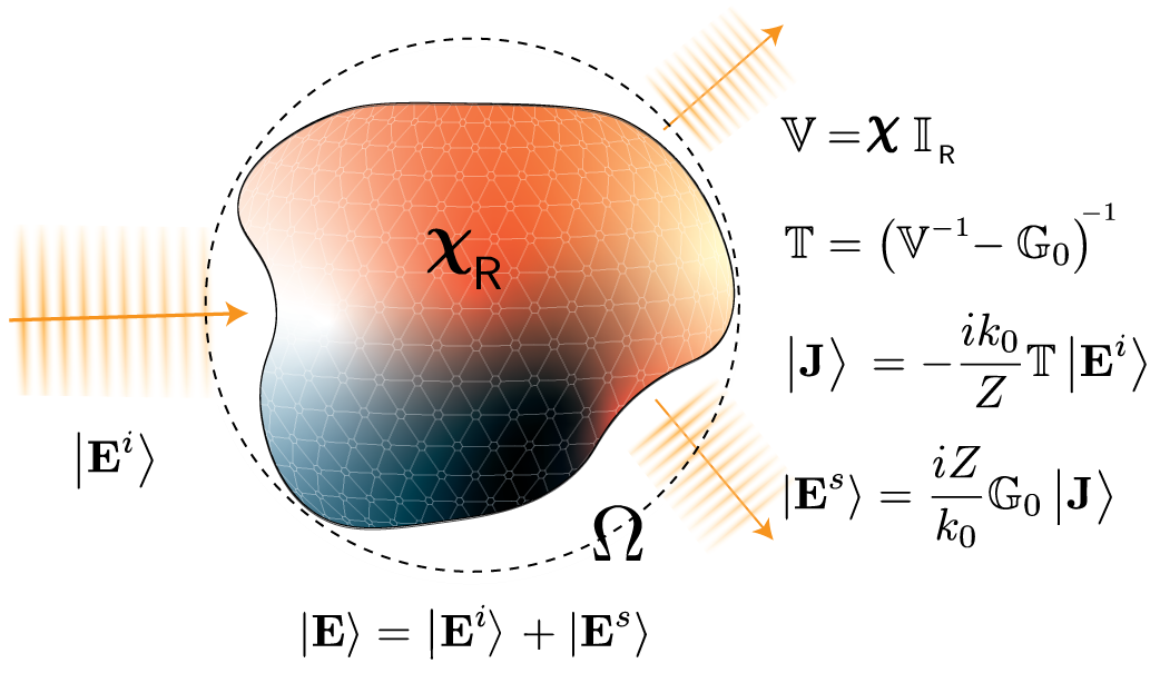
Figure 3: Schematic of scattering theory. The basis of scattering theory broadly rests on the existence, for each particular object (scattering potential), of an exact relation (the $\mathbb{T}$-operator) between incident (initial or free) electromagnetic fields and total (generated or net) polarization currents. Once this relation is known, the total electromagnetic field (the solution of Maxwell’s equations) is given by applying the Green’s function of the free (empty) domain $\mathbb{G}_{0}$ to the total current associated with the incident field.

At the finest level of detail that the design of a photonic device may be described (“true physics”), Maxwell’s wave equation associates each unique inhomogeneous dielectric profile $\mathbb{V}\left(\textbf{x},\omega\right)$ within a given domain $\Omega$ (assumed to enforce outgoing scattered fields [109, 110]), with a unique differential equation,

$$\nabla\times\nabla\times\textbf{E}\left(\textbf{x},\omega\right)-k_{0}^{2}~{}\mathbb{V}\left(\textbf{x},\omega\right)\cdot\textbf{E}\left(\textbf{x},\omega\right)=i\omega\mu_{0}~{}\textbf{J}^{f}\left(\textbf{x},\omega\right),$$ (1)

where $k_{0}=\omega/c=2\pi/\lambda$ and $\lambda$ is the free space wavelength. Unless $\mathbb{V}\left(\textbf{x},\omega\right)$ exhibits special symmetries, equations like (1) do not typically have complete closed form solutions, meaning that it is usually not possible to fully analyze how changes to the potential $\mathbb{V}$ alter the total field E beyond local expansions (derivatives) [111]. Nevertheless, this does not mean that the relation between $\mathbb{V}$ and E is completely opaque. In particular, suppose that $\textbf{J}^{f}\left(\textbf{x},\omega\right)=\textbf{0}$, and that the boundary conditions on $\Omega$ are set to describe an incident (incoming) electromagnetic field with electric component $\textbf{E}^{i}\left(\textbf{x},\omega\right)$. Introducing $\mathbb{I}_{{}_{\Omega}}\left(\textbf{x},\omega\right)$ as the identity operator, $\mathbb{I}_{{}_{\Omega}}\cdot\textbf{A}=\textbf{A}$, Eq. (1) may be rewritten as

$$\nabla\times\nabla\times\textbf{E}\left(\textbf{x},\omega\right)-k_{0}^{2}~{}\mathbb{I}_{{}_{\Omega}}\left(\textbf{x},\omega\right)\cdot\textbf{E}\left(\textbf{x},\omega\right)=$$

$$k_{0}^{2}~{}\left(\mathbb{V}\left(\textbf{x},\omega\right)-\mathbb{I}_{{}_{\Omega}}\left(\textbf{x},\omega\right)\right)\cdot\textbf{E}\left(\textbf{x},\omega\right).$$ (2)

The scheme of Eq. (2) is no different than that of Eq. (1) as applied to vacuum and the polarization “source” $\left(-ik_{0}/Z\right)$ $\left(\mathbb{V}\left(\textbf{x},\omega\right)-\mathbb{I}\left(\textbf{x},\omega\right)\right)\cdot\textbf{E}\left(\textbf{x},\omega\right)$, and as such, Eq. (2) implies an implicit integral relation on E (a volume integral formulation [112, 113]) that, while offering a distinct conceptual perspective [114] and possible computational advantages [115, 116, 117], is functionally equivalent to Maxwell’s equations. Setting $\mathbb{R}\left(\textbf{x},\omega\right)=\mathbb{V}\left(\textbf{x},\omega\right)-\mathbb{I}\left(\textbf{x},\omega\right)$ and decomposing $\textbf{E}\left(\textbf{x},\omega\right)$ as $\textbf{E}\left(\textbf{x},\omega\right)=\textbf{E}^{i}\left(\textbf{x},\omega\right)+\textbf{E}^{s}\left(\textbf{x},\omega\right)$ (with the $i$ superscript standing for “incident” and the $s$ superscript for “scattered”), regardless of what the shape specified by $\mathbb{R}\left(\textbf{x},\omega\right)$ actually is, $\textbf{E}\left(\textbf{x},\omega\right)$ must obey the self-referential (Lippmann-Schwinger [118] or Liouville-Neumann series relation [119, 120]) 

$$\textbf{E}^{s}\left(\textbf{x},\omega\right) =\int\limits_{{}_{\Omega}}\!\!d\textbf{x}^{\prime}~{}\mathbb{G}_{0}\left(\textbf{x},\textbf{x}^{\prime},\omega\right)\cdot\mathbb{R}\left(\textbf{x}^{\prime},\omega\right)\cdot\textbf{E}\left(\textbf{x}^{\prime},\omega\right)$$ (3)

$$=\int\limits_{{}_{\Omega}}\!\!\mathbb{G}_{0}\cdot\mathbb{R}\cdot\textbf{E}^{i}+\iint\limits_{{}_{\Omega}}\!\!\mathbb{G}_{0}\cdot\mathbb{R}\cdot\mathbb{G}_{0}\cdot\mathbb{R}\cdot\textbf{E}^{i}+\dots,$$

where, taking r to be $k_{0}\left(\textbf{x}-\textbf{x}^{\prime}\right)$, $r=\lVert\textbf{r}\rVert$, $\hat{\textbf{r}}\otimes\hat{\textbf{r}}$ to be the vector outer product of $\hat{\textbf{r}}=\textbf{r}/\lVert\textbf{r}\rVert$ with itself, and $\overline{\textbf{id}}$ the $3\times 3$ vector identity matrix,

$$\mathbb{G}_{0}\left(\textbf{x}-\textbf{x}^{\prime},\omega\right)=$$

$$\frac{k_{0}^{3}}{4\pi}\frac{e^{ir}}{r}\Bigg{[}\left(1+\frac{ir-1}{r^{2}}\right)\overline{\textbf{id}}~{}-\left(1+3\frac{ir-1}{r^{2}}\right)\hat{\textbf{r}}\otimes\hat{\textbf{r}}\Bigg{]},$$ (4)

is the vacuum Green’s function for the left hand side of Eq. (2) . (Note that an the additional factor of $k_{0}^{2}$ is included in Eq. (4) compared to its usual definition [123]. This is done so that every length that appears in the use of the Green’s function inside volume integrals is defined relative to the wavelength.) The mathematical form of Eq. (3) abstractly shows that $\textbf{J}\left(\textbf{x},\omega\right)=-\frac{ik_{0}}{Z}\mathbb{R}\left(\textbf{x},\omega\right)\cdot\textbf{E}\left(\textbf{x},\omega\right)$ must be regarded as the total polarization current density generated in response to $\textbf{E}^{i}\left(\textbf{x},\omega\right)$, and that Eq. (2) may be equivalently stated (in Fredholm integral form [113, 124]) as

$$\textbf{J}\left(\textbf{x},\omega\right)-\int\limits_{{}_{\Omega}}\!\!d\textbf{x}^{\prime}~{}\mathbb{R}\left(\textbf{x},\omega\right)\cdot\mathbb{G}_{0}\left(\textbf{x},\textbf{x}^{\prime},\omega\right)\cdot\textbf{J}\left(\textbf{x}^{\prime},\omega\right)=$$

$$-\frac{ik_{0}}{Z}~{}\mathbb{R}\left(\textbf{x},\omega\right)\cdot\textbf{E}^{i}\left(\textbf{x}^{\prime},\omega\right)=\textbf{J}^{i}\left(\textbf{x},\omega\right),$$ (5)

where $\bm{\mathrm{J}}^{i}$ is the “initial” polarization current density setup in response to the initial electric field, see Fig. 3.

Eqs. (3) and (5) rest at the foundation of scattering theory and definition of the $\mathbb{T}$-operator [125, 120] ($\mathbb{S}$-matrix [126, 127, 128]). Directly, via Eq. (3), every incident electric field is related to a specific polarization current density (the polarization that it generates) by

$$\mathbb{I}_{{}_{\mathsf{R}}}\textbf{E}^{i}\left(\textbf{x},\omega\right)=$$ (6)

$$\!\int\limits_{\mathsf{R}}\!d\textbf{x}^{\prime}~{}\left(\bm{\delta}\left(\textbf{x}-\textbf{x}^{\prime}\right)-\mathbb{G}_{0}\left(\textbf{x},\textbf{x}^{\prime},\omega\right)\cdot\mathbb{R}\left(\textbf{x}^{\prime},\omega\right)\right)\cdot\textbf{E}\left(\textbf{x}^{\prime},\omega\right)=$$

$$\!\frac{iZ}{k_{0}}\int\limits_{\mathsf{R}}\!d\textbf{x}^{\prime}~{}\left(\mathbb{R}^{-1}\left(\textbf{x}^{\prime},\omega\right)-\mathbb{G}_{0}\left(\textbf{x},\textbf{x}^{\prime},\omega\right)\right)\cdot\textbf{J}\left(\textbf{x}^{\prime},\omega\right),$$

where $\mathsf{R}$ is the subdomain of $\Omega$ where $\mathbb{R}\left(\textbf{x},\omega\right)\neq\textbf{0}$, the “material” extent of the scattering potential, and $\mathbb{R}^{-1}\left(\textbf{x},\omega\right)$ is the pseudo inverse of $\mathbb{R}$, the inverse over the subdomain where $\mathbb{R}$ is nonzero. Because $\mathbb{R}$ and $\mathbb{G}$ describe causal, passive, linear system responses, the total linear operator relating J to $\textbf{E}^{i}$ within $\mathsf{R}$ must be “invertible” [129, 130]. Accordingly, Eq. (3) delineates the existence of the inverse relation

$$\textbf{J}\left(\textbf{x},\omega\right)=-\frac{ik_{0}}{Z}\int_{{}_{\mathsf{R}}}d\textbf{x}^{\prime}~{}\mathbb{T}\left(\textbf{x},\textbf{x}^{\prime},\omega\right)\cdot\textbf{E}^{i}\left(\textbf{x}^{\prime},\omega\right)\Rightarrow$$ (7)

$$\mathbb{I}_{{}_{\mathsf{R}}}=\int\limits_{\mathsf{R}}d\textbf{x}^{\prime}~{}\left(\mathbb{R}^{-1}\left(\textbf{x}^{\prime},\omega\right)-\mathbb{G}_{0}\left(\textbf{x},\textbf{x}^{\prime},\omega\right)\right)\cdot\mathbb{T}\left(\textbf{x}^{\prime},\textbf{x}^{\prime\prime},\omega\right),$$

defining for each unique scattering potential $\mathbb{V}$ a unique linear response function $\mathbb{T}$ that relates any incident field $\textbf{E}^{i}$ to the polarization current density J that self-consistently solves Maxwell’s equations through Eq. (3). The operator relation governing the $\mathbb{T}$-operator, the Green’s function, and $\mathbb{V}$ given in Eq. (7), like Eqs. (3) and (6), is fully equivalent to Maxwell’s equations and serve as an advantageous starting point for deriving conserved quantities.

From Eq. (6), relatively little must be done to reframe the determination of an optimal scattering object $\mathbb{V}$ in terms of the polarization current density. First, by integrating against the characteristic function of any other known subdomain $\mathsf{P}$ of $\Omega$, together with a local “polarization” projection matrix $\mathbb{P}\left(\textbf{x},\omega\right)$—a linear response that does not mix distinct spatial points—the integration domains appearing in Eq. (5) are shifted from $\mathsf{P}$ to $\mathsf{R}\cap\mathsf{P}$, standing for the common spatial volume of $\mathsf{R}$ and $\mathsf{P}$. Next, by applying this result against the conjugate of $\textbf{J}\left(\textbf{x},\omega\right)$ itself, for any $\mathbb{P}\left(\textbf{x},\omega\right)$ Eq. (6) is transformed into

$$\int\limits_{{}_{\mathsf{P}}}\!\!d\textbf{x}~{}~{}\textbf{J}^{*}\left(\textbf{x},\omega\right)\cdot\mathbb{P}\left(\textbf{x},\omega\right)\cdot\\ \left(\underline{\mathbb{R}}^{-1}\left(\textbf{x},\omega\right)\cdot\textbf{J}\left(\textbf{x},\omega\right)-\int\limits_{{}_{\Omega}}\mathbb{G}_{0}\left(\textbf{x}-\textbf{x}^{\prime},\omega\right)\cdot\textbf{J}\left(\textbf{x}^{\prime},\omega\right)\right)=\\ -\frac{ik_{0}}{Z}\int\limits_{{}_{\mathsf{P}}}\!\!d\textbf{x}~{}\textbf{J}^{*}\left(\textbf{x},\omega\right)\cdot\mathbb{P}\left(\textbf{x},\omega\right)\cdot\textbf{E}^{i}\left(\textbf{x}\right);$$ (8)

where, crucially, the dependence of the domains of integration on the spatial structure of $\mathbb{R}\left(\textbf{x},\omega\right)$ has been removed. Based on the fact that $\mathbb{R}\left(\textbf{x},\omega\right)=\textbf{0}$ implies that $\textbf{J}\left(\textbf{x},\omega\right)=\textbf{0}$, the content of Eq. (8) is unchanged for any choice of response function $\underline{\mathbb{R}}^{-1}$ on $\Omega$ so long as $\underline{\mathbb{R}}^{-1}\left(\textbf{x},\omega\right)=\mathbb{R}^{-1}\left(\textbf{x},\omega\right)$ when $\textbf{x}\in\mathsf{R}$. If $\mathbb{V}\left(\textbf{x},\omega\right)$ may only take on a single $3\times 3$ matrix form distinct from 0, as is usually true in photonics when designing a device composed of a single material , then Eq. (8), with $\bm{\chi}\left(\omega\right)$ denoting the electric susceptibility matrix of the material, may be further simplified by setting $\underline{\mathbb{R}}^{-1}\left(\textbf{x},\omega\right)=\bm{\chi}^{-1}\left(\textbf{x},\omega\right)$, see Eq. (10) below. The only quantity in Eq. (8) that is not typically known from the outset of a design problem is $\textbf{J}\left(\textbf{x},\omega\right)$. At the same time, because the physics of Maxwell’s equation is incorporated through $\mathbb{G}_{0}$, the true behaviour of the dielectric scattering potential is incorporated through $\bm{\chi}^{-1}$, and the self-consistency of viewing $\textbf{J}\left(\textbf{x},\omega\right)$ as the electric polarization current density resulting from the electromagnetic field given by $\textbf{E}^{i}\left(\textbf{x},\omega\right)$ is incorporated by association with Eq. (3), any vector field that respects Eq. (8) for all possible choices of $\mathbb{P}\left(\textbf{x},\omega\right)$ actually defines an effective medium scattering structure [43] (a mix between the material properties asserted by $\mathbb{V}\left(\textbf{x},\omega\right)$ and the background).

Optimization bounds—The observation that every constraint of the form given by Eq. (8) applies to any structure of a given material within $\Omega$ implies that a great number of common photonic objectives can be stated as quadratically constrained quadratic programs (QCQPs) [44], and, in turn, bounded using standard relaxation techniques from optimization theory [107]. The connection between Eq. (8) and QCQPs is most easily seen by switching to a more compact notation. Making use of the fact that integration may be viewed as an inner product for fields or functions [132] , with $\left<\textbf{A}\big{|}\textbf{B}\right>=\int d\bm{\mathrm{x}}~{}\textbf{A}^{*}(\bm{\mathrm{x}})\cdot\textbf{B}(\bm{\mathrm{x}})$ denoting the standard complex-conjugate inner product, Eq. (8) may be written in bra-ket form as

$$\left<\textbf{T}\right|\mathbb{P}\left(\bm{\chi}^{-1}-\mathbb{G}_{0}\right)\left|\textbf{T}\right>=\left<\textbf{T}\right|\mathbb{P}\left|\textbf{E}^{i}\right>,$$ (9)

with $\left|\textbf{T}\right>=\frac{iZ}{k_{0}}\left|\textbf{J}\right>=\mathbb{T}\left|\textbf{E}^{i}\right>$, leading to the following equivalent adjoint quadratic constraint equations

$$\imaginary\left(\left<\textbf{E}^{i}\right|\mathbb{P}\left|\textbf{T}\right>\right)-\left<\textbf{T}\right|\left[\left(\bm{\chi}^{-1\dagger}-\mathbb{G}_{0}^{\dagger}\right)\mathbb{P}\right]^{\mathsf{A}}\left|\textbf{T}\right>=0,$$

$$\real\left(\left<\textbf{E}^{i}\right|\mathbb{P}\left|\textbf{T}\right>\right)-\left<\textbf{T}\right|\left[\left(\bm{\chi}^{-1\dagger}-\mathbb{G}_{0}^{\dagger}\right)\mathbb{P}\right]^{\mathsf{S}}\left|\textbf{T}\right>=0,$$ (10)

In these expressions, and the proceeding text, $\mathsf{S}$ superscripts will be used to mark the Hermitian (symmetric) part of the contained linear response function $\textbf{M}^{\mathsf{S}}=\left(\textbf{M}+\textbf{M}^{\dagger}\right)/2$, and $\mathsf{A}$ superscripts will be used to denote the anti-symmetric part, $\textbf{M}^{\mathsf{A}}=\left(\textbf{M}-\textbf{M}^{\dagger}\right)/2i$, so that, like a complex number, $\textbf{M}=\textbf{M}^{\mathsf{S}}+i~{}\textbf{M}^{\mathsf{A}}$ .

When $\mathbb{P}$ is set to the domain identity $\mathbb{I}_{{}_{\Omega}}$, the first relation of Eq. (10) is a statement of the conservation of real power within the domain [40]: the power drawn by the polarization current from the field, the inner product $\imaginary\left(\left<\textbf{E}^{i}\big{|}\textbf{T}\right>\right)$, must equal the sum of the power lost by the polarization current to material extinction [135],

$$\left<\textbf{T}\right|\left(\bm{\chi}^{-1\dagger}\right)^{\mathsf{A}}\left|\textbf{T}\right>=\!\int\limits_{\Omega}\!\!d\textbf{x}~{}\textbf{T}^{*}\left(\textbf{x}\right)\cdot\frac{\imaginary\left[\mathbb{V}\left(\textbf{x},\omega\right)\right]~{}}{\lVert\mathbb{V}\left(\textbf{x},\omega\right)\rVert^{2}}\cdot\textbf{T}\left(\textbf{x}\right)$$ (11)

and to outgoing radiation [136]

$$\left<\textbf{T}\right|\mathbb{G}_{0}^{\mathsf{A}}\left|\textbf{T}\right>=\!\iint\limits_{\Omega}\!\!d\textbf{x}^{\prime}d\textbf{x}~{}\textbf{T}^{*}\left(\textbf{x}^{\prime}\right)\cdot\imaginary\left[\mathbb{G}_{0}\left(\textbf{x}^{\prime},\textbf{x},\omega\right)\right]\cdot\textbf{T}\left(\textbf{x}\right).$$ (12)

The second relation contained in Eq. (10), as illustrated further below, makes the related statement that reactive power must also be conserved, see Refs. [137, 39, 111]. Together, these equalities impose minimum requirements on the characteristics of $\mathbb{V}$ and spatial extent of the domain $\Omega$—through $\mathbb{G}_{0}$ which is limited to $\Omega$—needed to achieve resonant response. That is, depending on the material the device will be made of and the spatial volume that it may possibly occupy, there may be strong limits on the degree to which the amplitude and phase of J relative to $\textbf{E}^{i}$ may be tuned.

Recalling from Eq. (3) that the field and induced polarization currents are linearly related by $\left|\textbf{E}\right>=\left|\textbf{E}^{i}\right>+\frac{iZ}{k_{0}}\mathbb{G}_{0}\left|\textbf{J}\right>$, it follows that any physical process described by quadratic field terms—including the fundamental time-averaged power-transfer quantities of absorption $k_{0}\left<\textbf{E}\right|\bm{\chi}^{\mathsf{A}}\left|\textbf{E}\right>/2Z$, extraction $\real\left(\left<\textbf{E}^{i}\big{|}\textbf{J}\right>\right)/2$ and scattering $Z\left<\textbf{J}\right|\mathbb{G}_{0}^{\mathsf{A}}\left|\textbf{J}\right>/2k_{0}$, which rest as the basic figures of merit for the design of antennas [138, 139, 106], light trapping devices [63, 140, 141, 142, 143, 144], and optoelectronic coupling [145, 146, 147, 9]—can be considered as a quadratic objective. In this language, taking $\mathtt{f}_{0}\left(\left|\textbf{T}\right>\right)$ to denote some quadratic function of the polarization, and K a complete set of constraints  the goal of maximizing (resp. minimizing) any such objective through material structuring may be formulated as

$$\max_{\left|\textbf{T}\right>}~{}\left(\text{resp.}\min_{\left|\textbf{T}\right>}\right)~{}\mathtt{f}_{0}\left(\left|\textbf{T}\right>\right)$$

$$\text{such that}~{}\forall k\in\text{K}$$

$$\real\left(\left<\textbf{E}\right|\mathbb{P}_{k}\left|\textbf{T}\right>\right)-\left<\textbf{T}\right|\left[\mathbb{P}_{k}\left(\bm{\chi}^{-1\dagger}-\mathbb{G}_{0}^{\dagger}\right)\right]^{\mathsf{S}}\left|\textbf{T}\right>=0,$$

$$\imaginary\left(\left<\textbf{E}\right|\mathbb{P}_{k}\left|\textbf{T}\right>\right)-\left<\textbf{T}\right|\left[\mathbb{P}_{k}\left(\bm{\chi}^{-1\dagger}-\mathbb{G}_{0}^{\dagger}\right)\right]^{\mathsf{A}}\left|\textbf{T}\right>=0,$$ (13)

which is the form of a quadratically constrained quadratic program (QCQP). Because the enforcement of fewer constraints always leads to maxima of greater or equal value (resp. minima of equal or smaller value) in any optimization, the imposition of any collection of constraints that can be formed from K may be used to construct a relaxed QCQP that contains the feasible set of Eq. (13)—an optimization with maxima (resp. minima) at least as large (resp. small) as Eq. (13) . Any bound on such a relaxed program is necessarily a bound on Eq. (13), and so, by applying any additional relaxation such as Lagrange duality or semi-definite programming [44], it is possible to obtain limits on the physically realizable values of $\mathtt{f}_{0}\left(\left|\textbf{T}\right>\right)$ that universally apply to any possible material structure within $\Omega$, c.f. Refs. [39, 111, 40, 41, 42, 150, 151, 43, 44]. As highlighted by the expositive examples below, the extent to which these limits incorporate various physical phenomena may be tuned by selecting, either by intuition or algorithm [40], the collection of constraints ($\mathbb{P}_{k}$ projections) that are concurrently imposed, and, in contrast to many traditional approaches to limits, where individual components of an expression are bounded and then subsequently summed or composed to form a global bound, the optimization framework of Eq. (13) properly describes interactions between constraints.

Although no further refinements of Eq. (13) will be examined hereafter, it should be noted that this basic optimization bounds approach can, and in certain cases should, be extended in at least two meaningful ways. First, by moving to complex frequencies as described in Ref. [18] and Ref. [152], it is possible to adapt Eq. (13) to treat both broadband and temporal problems. Detailed accounts of these modifications can be found in Refs. [42, 153]. Second, in situations involving multiple incident fields or scattering objectives, including applications to multi-functional devices—design objectives like optical multiplexing [154, 155, 156], meta-optic imaging components [157, 158, 37, 36] and optical computing [159, 160, 161]—it is necessary to broaden the scope of the quadratic equalities included in Eq. (13) to properly account for the additional challenges presented by the need to engineer multiple field transformations within a common structure. A full account of these alterations is given in Ref. [43].

Representative scattering limits

In order to build intuition and provide context, the ensuing section reviews three increasingly complex tutorial applications of Eq. (13) to set fundamental upper bounds on optical response. Beginning with the conservation of real power, focusing on the equivalent problems of maximizing thermal emission or net absorption, the modal characteristics of $\mathbb{G}_{0}^{\mathsf{A}}$ in relation to Eq. (10) are shown to reproduce familiar asymptotic results from quasi-statics and ray optics. However, because optimization limits do not rely on the validity of such approximate forms, calculated bounds are also seen to be meaningfully applicable to intermediate and hitherto inaccessible wavelength-scale regimes. Next, by further imposing that reactive power be conserved, simultaneously enforcing the two constraints in Eq. (10) through $\mathbb{P}=\mathbb{I}_{{}_{\Omega}}$, limits on achievable scattering cross sections are found to anticipate conditions on the size of the design domain under which resonant response is possible for a given material choice. Finally—as exemplified through calculations of bounds on scattering cross sections, radiative emission from a dipolar source in the near field of body, and power splitting—the set of integral relations contained in the relaxations of Eq. (13) has the effect of defining the degree to which the physics of scattering theory is enforced, and correspondingly, the number and types of integral constraints imposed in calculating optimization bounds function as complements to the different number and types of optimization degrees of freedom that may be used in structural optimization. For proper comparison against realizable devices, constraints must be selected in a manner that “resolves” the wave physics of the problem, e.g., accurate limits on phenomena dominated by rapidly decaying (evanescent) fields require a greater number of local constraints. In almost all of these representative applications, objective values obtained through structural “topology” (or “density”) optimization are found to come within an order of magnitude of their determined limit values [19].

Real power conservation—As a first application of Eq. (13), we review how the conservation of real power sets an upper bound on thermal radiation and, by reciprocity, angle-integrated absorption. At a microscopic level, thermal emission results from stochastically fluctuating electrical currents in matter [162, 163], with the precise relationship between temperature, energy dissipation, and field fluctuations in an object in equilibrium determined by the fluctuation-dissipation theorem [164]. The basis for such a relation may be intuitively understood from Brownian motion [165]. A particle traveling in a fluid experiences a dissipation of its net velocity due to collisions with the constituent particles of the surrounding fluid. Complementarily, these collisions impart momentum, causing fluctuations in the position of the particle about its average location, $\langle x^{2}\rangle=2Dt$, where $t$ is the elapsed time and $D$ is the diffusion coefficient, which by the Stokes-Einstein relation $D=k_{B}T/\gamma$ is inversely proportional to the the drag (dissipation) coefficient $\gamma$ [166]. An analogous relation is seen in the Nyquist formula for Johnson noise, $\langle V^{2}\rangle=4Rk_{B}Td\nu$, where $V$ is the voltage between the terminals of an open circuit (e.g. a conductive wire), $R$ the electrical resistance, and $d\nu$ a frequency interval [167]. The fluctuation-dissipation theorem generalizes and formalizes these observations. For the electromagnetic settings considered here [123],

$$\underbrace{\left\{J_{i}(\mathbf{x},\omega)J_{j}^{*}(\mathbf{x}^{\prime},\omega^{\prime})\right\}_{T}}_{\text{fluctuation}}=$$ (14)

$$\frac{\omega\epsilon_{0}}{2\pi}\coth\left(\frac{\hslash\omega}{2k_{B}T}\right)\underbrace{\bm{\chi}_{ij}^{\mathsf{A}}(\mathbf{x},\omega)}_{\text{dissipation}}~{}\delta_{ij}~{}\delta(\mathbf{x}-\mathbf{x}^{\prime})~{}\delta(\omega-\omega^{\prime}),$$

where $\left\{\dots\right\}$ denotes a thermal ensemble average: Fluctuations in the current density are point correlated and proportional to the dissipative part of the electric susceptibility (the optical conductivity).

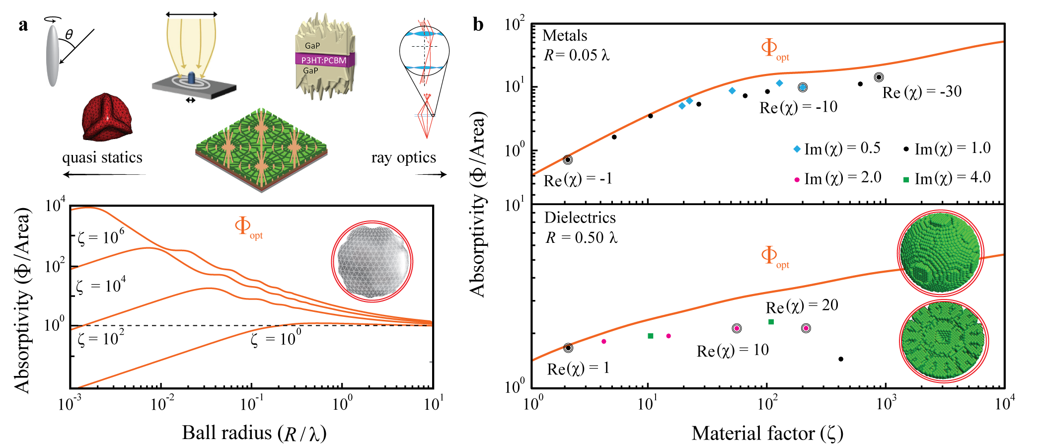
Figure 4: Bounds on angle-integrated absorption based on the conservation of real power. Panel a illustrates the results of Eq. (19) as a function of the size (radius $R/\lambda$) of a spherically bounded design volume for several values of the material factor $\zeta=\lVert\chi\rVert^{2}/\imaginary\left(\chi\right)$. Notably, in transitioning between very small design volumes, $R\ll\lambda$, and very large design volumes, $R\gg\lambda$, Eq. (19) is seen to smoothly blend the familiar $\propto V$ and $\propto A$ limits of quasi-static and ray-optic (blackbody) approximations. Above panel a, a collection of representative use cases of radiative absorption are included to give a sense of the range of length scales covered below. Working from left to right, these images are taken from Ref. [168], Ref. [135], Ref. [147], Ref. [142], and Ref. [169]. Panel b depicts a comparison of $\Phi_{opt}$ against performance values obtained by computational design methods for two set domain sizes, $R/\lambda=1/20$ for metals ($\real\left(\chi\right)<0$) and $R/\lambda=1/2$ for dielectrics ($\real\left(\chi\right)>0$). Unless additional constraints are included, findings for dielectric materials limited to small domains, and findings for metals in large domains, exhibit substantially larger disagreement.

Exploiting this relation and the incoherent nature of the fluctuations, the net emitted power may be expressed as a sum over independent radiative channels. Generally, the instantaneous power emitted by a current source is

$$P_{rad}=-\int_{\mathsf{R}}\mathbf{J}(\mathbf{x},t)\cdot\mathbf{E}(\mathbf{x},t)$$ (15)

where the minus sign results from the convention of emitted power. Switching to the spectral domain , and assuming that the collection of fluctuating dipolar sources distributed throughout the body satisfy Eq. (14), the thermal power radiated by a body held at a constant temperature $T$ (c.f. [171, 125, 136]) is given by

$$\{P_{rad}\}_{T} =\int\limits_{0}^{\infty}d\omega~{}\Pi(\omega,T)~{}\underbrace{\frac{2}{\pi}\text{Tr}\,[\mathbb{G}_{0}^{\mathsf{A}}(\mathbb{T}^{\mathsf{A}}-\mathbb{T}^{\dagger}\mathbb{G}_{0}^{\mathsf{A}}\mathbb{T})]}_{\Phi(\omega)}$$ (16)

where $\Pi(\omega,T)=\frac{\hslash\omega}{\exp(\hslash\omega/\left(k_{B}T\right))-1}$ is the Planck thermal occupation function, and $\Phi(\omega)$ the corresponding angle-integrated spectral transfer function (absorption or emission) of the body; the Tr symbol denotes a trace over both the position and polarization indices of the dipole sources, i.e. the complete set of indices of the enclosed operators.

In the breakup of Eq. (16), the $\mathbb{T}^{\mathsf{A}}-\mathbb{T}^{\dagger}\mathbb{G}_{0}^{\mathsf{A}}\mathbb{T}$ term contained in $\Phi$ constitutes an algebraic description of absorption, Eq. (11), expressed as the subtraction of radiated power $\mathbb{T}^{\dagger}\mathbb{G}_{0}^{\mathsf{A}}\mathbb{T}$, Eq. (12), from the total extracted (extinction) power $\mathbb{T}^{\mathsf{A}}$. This association is no accident: as a consequence of reciprocity, evaluating the trace over a (delocalized) basis of waves incident on the body changes the interpretation of $\Phi$ from the net emitted power due to dipolar sources within the object (thermal emission) to the net power absorbed in the body due to incident plane waves (angle-integrated absorption), but the algebraic form of $\Phi$ remains unaltered. Because $\mathbb{G}_{0}^{\mathsf{A}}$ describes how outgoing radiation carries power away from an object into the surrounding environment [129, 136], a natural basis in which to evaluate the trace is the eigenmode expansion

$$\mathbb{G}_{0}^{\mathsf{A}}=\sum_{n}\rho_{n}\left|\mathbf{Q}_{n}\right>\left<\mathbf{Q}_{n}\right|,$$ (17)

with each of the radiative coefficients $\rho_{n}$ nonnegative by passivity. Setting $\left|\mathbf{T}_{n}\right>=\mathbb{T}\left|\mathbf{Q}_{n}\right>$ , $\Phi$ becomes

$$\Phi=\frac{2}{\pi}\sum_{n}\rho_{n}\left(\imaginary\left[\left<\mathbf{Q}_{n}|\mathbf{T}_{n}\right>\right]-\left<\mathbf{T}_{n}\right|\mathbb{G}_{0}^{\mathsf{A}}\left|\mathbf{T}_{n}\right>\right).$$ (18)

Even without the imposition of a single constraint, the form of Eq. (18) places fairly strong restrictions on the extent to which the net absorption (resp. emission) cross section of an object can be enhanced compared to its geometric cross section [136]. In order to optimize absorption it is clear from Eq. (18) that each radiative mode must generate a strong polarization: $\imaginary\left[\left<\mathbf{Q}_{n}|\mathbf{T}_{n}\right>\right]$ is the extracted power. However, the generation of these currents necessarily leads to radiative losses, $\left<\mathbf{T}_{n}\right|\mathbb{G}_{0}^{\mathsf{A}}\left|\mathbf{T}_{n}\right>$, which grow relatively in strength as the size of the domain increases through the growth of the $\rho_{n}$ radiative coupling coefficients [136, 97].

As a first example of optimization bounds, we analyze the maximization of $\Phi$ subject to the constraint that real power is conserved:

$$\max_{\{\left|\mathbf{T}_{n}\right>\in\Omega\}}~{}\frac{2}{\pi}\sum_{n}\rho_{n}\left(\imaginary\left[\left<\mathbf{Q}_{n}|\mathbf{T}_{n}\right>\right]-\left<\mathbf{T}_{n}\right|\mathbb{G}_{0}^{\mathsf{A}}\left|\mathbf{T}_{n}\right>\right)$$

$$\text{such that}~{}\forall n$$

$$\imaginary\left[\left<\mathbf{Q}_{n}|\mathbf{T}_{n}\right>\right]-\left<\mathbf{T}_{n}\right|\left(\bm{\chi}^{-1\dagger}-\mathbb{G}_{0}^{\dagger}\right)^{\mathsf{A}}\left|\mathbf{T}_{n}\right>=0,$$ (19)

effectively the simplest version of Eq. (13). Due to the form of $\Phi$, the only difference between the objective and constraint in Eq. (19) is the material loss term $\lVert\mathbf{T}_{n}\rVert^{2}/\zeta$, with the factor $\zeta\equiv\lVert\chi\rVert^{2}/\imaginary\left[\chi\right]$ quantifying the maximum magnitude that the polarization current density can achieve relative to the incident electric field [173]. Simply, to maintain equilibrium, the net (integrated) power extracted by the object at each frequency must be perfectly balanced by the sum of two possible loss mechanisms: the absorption of power into material degrees of freedom ($\bm{\chi}^{-1\dagger\mathsf{A}}$), here considered to be an infinitely large thermal bath [174], and power re-radiated (scattered or reflected) back into the ambient environment ($\mathbb{G}_{0}^{\mathsf{A}}$).

Applying the relaxation of Lagrange duality (c.f. Refs. [107, 175, 67, 111, 44]), the optimal objective value of Eq. (19) can be expressed as

$$\Phi_{opt}=\frac{1}{2\pi}\sum_{n}\begin{cases}~{}1&\zeta\geq\frac{1}{\rho_{n}}\\ \frac{4\zeta\rho_{n}}{(1+\zeta\rho_{n})^{2}}&\zeta<\frac{1}{\rho_{n}}\\ \end{cases}\leftrightarrow\begin{cases}~{}1&\tau_{m,n}\geq\tau_{r,n}\\ \frac{4\tau_{m,n}\tau_{r,n}}{(\tau_{r,n}+\tau_{m,n})^{2}}&\tau_{m,n}<\tau_{r,n}\\ \end{cases},$$ (20)

with $\leftrightarrow$ marking associations, $\tau_{r,n}\leftrightarrow 1/\rho_{n}$ and $\tau_{m,n}\leftrightarrow\zeta$, with a coupled-mode analysis, Box. 1. The surprising simplicity of $\Phi_{opt}$ as arising from a sum over independent channel contributions follows from the fact that, absent other scattering constraints (beside real power conservation), the optimal bound polarization currents end up becoming diagonal in the basis of radiation states (the eigenbasis of $\mathbb{G}_{0}^{\mathsf{A}}$), $\ket{\bm{\mathrm{T}}_{n}}\approx c_{n}\left|\mathbf{Q}_{n}\right>$ (neglecting non-radiative terms that yield minor modifications), with the maximum bound polarization response $\lVert c_{n}\rVert\leq\min\left\{\frac{1}{2\rho_{n}},\zeta\right\}$ in each channel.

A trio of plots of $\Phi_{opt}$, bounding angle-integrated absorption (equivalently emission) for bodies enclosed in a spherical ball of radius $R$, are shown in Fig. 4. Beyond the exact quantitative predictions appearing in a, and the excellent agreement with computationally designed structures appearing in b (see Refs. [116, 136] for details), it is seen that the mere conservation of net real power is sufficient for Eq. (19) to inherently reproduce fundamental quasi-static and blackbody behavior. In the limit of a small design volume, $\zeta\rho_{n}\ll 1$ (resp. $\tau_{m,n}\ll\tau_{r,n}$) for all $n$, $\Phi_{opt}$ is seen to exhibit a volumetric scaling consistent with the assumption that the magnitude of all generated polarization currents can grow as large as material loss allows: as the volume grows, so does the available power in each channel, and hence so should the polarization response. However, due to the necessary coupling of these currents with radiative states, volumetric growth cannot persist indefinitely. Eventually, in each index of Eq. (18), growth in $\rho_{n}$ (resp. decay in $\tau_{r,n}$) causes radiative losses to discordantly overwhelm net extracted power if the magnitude of $\left|\mathbf{T}_{n}\right>$ (resp. the material lifetime $\tau_{m,n}$) becomes too large, leading the associated channel (index) to enter the saturation condition of Eq. (20), visible in Fig. 4 as the onset of steps. As an increasing number of channels saturate, volumetric scaling begins to asymptotically transition to area scaling, regardless of the supposed value of $\zeta$. Directly, the black-body limit equating absorption and geometric cross sections appears out of Eq. (19), irrespective of assumed material properties.

The behaviors of the $\rho_{n}$ radiative expansion coefficients also have interesting implications for antenna design [105, 176]. For any excitation contained within $\Omega$, the largest radiative coefficient $\rho_{n}$ in Eq. (17) sets a lower bound on the radiative lifetime, $\tau_{r}$, and consequently, a lower bound on the radiative quality factor $Q_{r}=\omega\tau_{r}/2$. In the limit of a deeply subwavelength design volume, the largest $\rho_{n}$ (the dipole coefficient) scales $\propto\left(k_{0}R\right)^{3}$, setting a lower bound on the radiative quality factor $\propto\left(k_{0}R\right)^{-3}$ [62, 177, 178]. This lower bound on $Q_{r}$, known as the Chu limit ($Q_{\mathrm{rad}}\geq\frac{1}{k_{0}R}+\frac{1}{(k_{0}R)^{3}}$ [178]), correspondingly sets an upper limit on antenna bandwidth that restricts processing speed [179].

Finally, as suggested above, the sum expression for $\Phi_{opt}$ given by Eq. (20) is completely analogous to a modal description of absorption by non-interacting excitations and, as one might expect, under this analogy the channel saturation condition of $\zeta\rho_{n}=1$ is exactly the rate-matching condition $\tau_{r,n}=\tau_{m,n}$ between radiative and material lifetimes. Consequently, it is accurate to interpret Eq. (20) as a model wherein an idealized object independently extracts power from each of the radiative (multipole) states in a physically optimal way, with $\rho_{n}$ and $\zeta$ setting limits on the associated coupled-mode radiative and dissipation rates for every channel. As discussed in greater detail below, this perspective implicitly assumes that resonant response is achievable in each individual channel, and that attaining resonant response in one channel has no implications for any other. Neither assumption is typically true in practice.

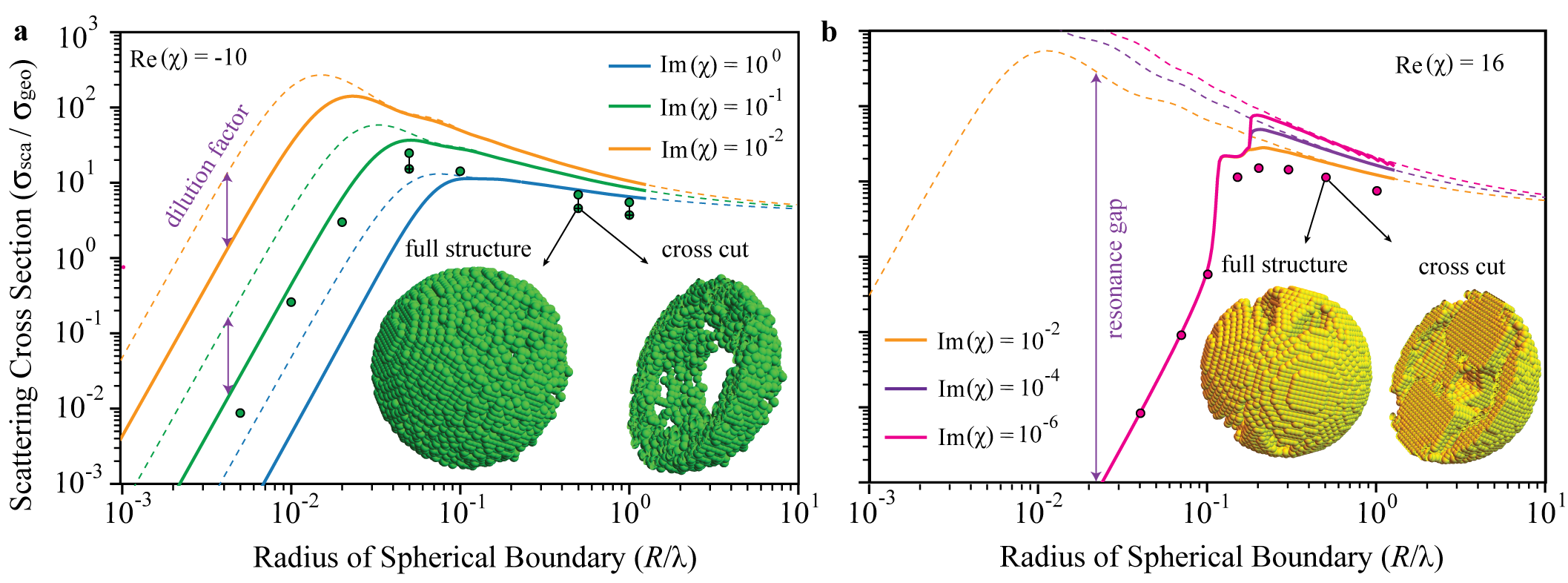
Figure 5: Bounds on scattering cross sections based on the conservation of total power. Panels a and b, taken from Ref. [111], depict the results of Eq. (22) as a function of the size (radius $R/\lambda$) of a spherically bounded design volume for two representative values of $\real\left[\chi\left(\omega\right)\right]$ near optical frequencies (a near plasmonic metal a and a strong dielectric b.) Dashed lines result from only imposing the conservation of real power; solid lines result from additionally imposing the conservation of reactive power. The dots appearing in both panels mark scattering cross sections achieved in actual geometries discovered by numeric (inverse) design, for $\chi=-10+i10^{-1}$ and $\chi=16+i10^{-6}$ respectively. For the metal structures in a, aligned cross-hatched dots result from binarizing the discovered permittivity profiles, which are otherwise allowed to take on “gray-scale” values [19]. Two sample structures are shown as insets, with the planewave incident from the more solid side of both designs, from the left in a, from the right in b, and aligned along the left-right symmetry axis. Again, in the limit that $R/\lambda\gg 1$ or $R/\lambda\ll 1$ the calculated bounds approach the scaling predictions of ray optics (geometric cross sections) and quasi-static scattering ($\propto V^{2}$), irrespective of the electric susceptibility. The inclusion of reactive power conservation for strong metals ($\real\left[\chi\left(\omega\right)\right]\ll-3$) confined to small design volumes ($R/\lambda\ll 1$) shows that the structuring needed to achieve resonant scattering away from the plasmon condition of $\real\left[\chi\left(\omega\right)\right]=-3$ reduces achievable material scaling characteristics—the appearance of “dilution factors”. The of effect total power conservation on obtained limits for dielectric materials confined to subwavelength domains is more radical—causing the appearance of “resonance gaps”—leading to the general conclusion that scattering cross section enhancements surpassing $\approx 200$ should not be expected for near optical frequencies.

Total power conservation—Given the remarkable agreement observed in Fig. 4b between the absorption characteristics of structures obtained by computational techniques and the associated bounds, it is natural to wonder whether related conclusions can be drawn for all basic scattering quantities; namely, to what extent are the results of current inverse methods explained by the basic necessity of conserving power?

Recalling that the power scattered from an initial electric field $|\mathbf{E}^{i}\rangle$ at a single frequency $\omega$ is [120, 111]

$$P_{sct} =\frac{k_{0}}{2Z}\left<\mathbf{E}^{i}\right|\left[\mathbb{T}^{\mathsf{A}}-\mathbb{T}^{\dagger}\left(\mathbb{V}^{-1\dagger}\right)^{\mathsf{A}}\mathbb{T}\right]\left|\mathbf{E}^{i}\right>,$$ (21)

the problem of maximizing the scattering cross section of an object contained within a design volume $\Omega$ becomes the optimization statement

$$\max_{\left|\mathbf{T}\right>\in\Omega}~{}\frac{k_{0}}{2Z}\left[\imaginary\left(\left<\mathbf{E}^{i}|\mathbf{T}\right>\right)-\left<\mathbf{T}\right|\bm{\chi}^{-1\dagger\mathsf{A}}\left|\mathbf{T}\right>\right]$$

such that

$$\imaginary\left(\left<\textbf{E}^{i}|\textbf{T}\right>\right)-\left<\textbf{T}\right|\left(\bm{\chi}^{-1\dagger}-\mathbb{G}_{0}^{\dagger}\right)^{\mathsf{A}}\left|\textbf{T}\right>=0,$$

$$\real\left(\left<\textbf{E}^{i}|\textbf{T}\right>\right)-\left<\textbf{T}\right|\left(\bm{\chi}^{-1\dagger}-\mathbb{G}_{0}^{\dagger}\right)^{\mathsf{S}}\left|\textbf{T}\right>=0,$$ (22)

where $|\mathbf{E}^{i}\rangle$ is the electric field of an incident plane wave and, as before, $\left|\mathbf{T}\right>=\mathbb{T}\left|\mathbf{E}^{i}\right>$ so that $\left(-ik_{0}/Z\right)\left|\mathbf{T}\right>=\left|\mathbf{J}\right>$ is the resulting electric polarization current density in the object. If only the conservation of real power is imposed, the solution of Eq. (22) closely mirrors the coupled-mode expression for integrated emission given by Eq. (20). However, as is clear from a comparison of the solid (enforcing total power conservation) and dashed (enforcing only real power conservation) lines of Fig. 5 (particularly b), the inclusion of the global reactive power constraint, the final line of Eq. (22), leads to substantially tighter limits , and under the imposition of this additional constraint, barring the single channel asymptotic examined in Box. 1, the solution of Eq. (22) does not have a simple semi-analytic form. The physical mechanism underlying these differences is the appearance of phase information. Paralleling the well-known response characteristics of a simple harmonic oscillator, when only the conservation of real power is enforced there is a bound on the relative magnitude of $\left|\textbf{T}\right>$ set by material absorption and radiative emission. All information about the relative phase offset of the response, partially set by $\real\left[\chi\left(\omega\right)\right]$, is ignored. Once the need to conserve reactive power is taken into account, physical restrictions are placed on both the relative magnitude and phase of the response [137, 39, 111]. These restrictions can either limit, or even exclude, resonant response  in certain situations.

Box 1: Single-channel asymptotics (antenna cross sections)
 

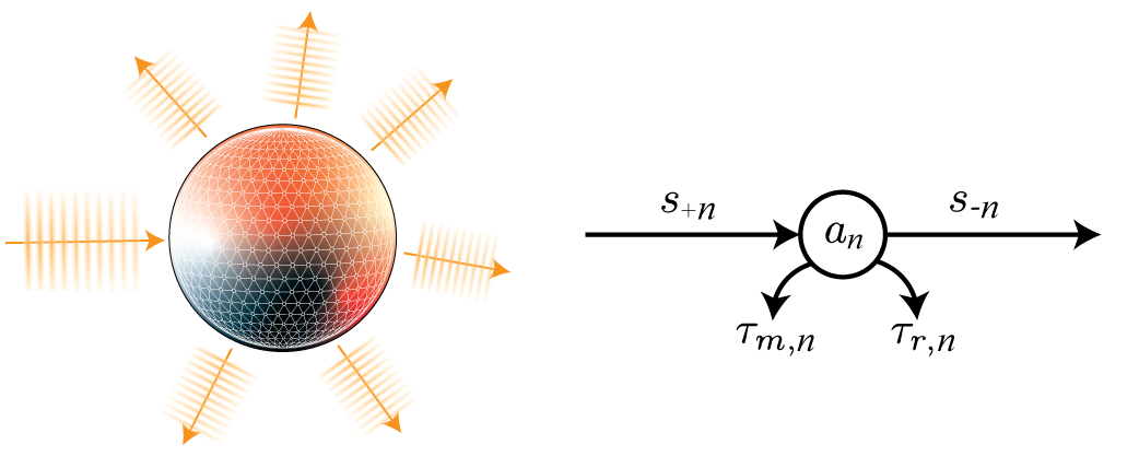
Figure 6: Schematic of coupled-mode theory. The figure, adapted from Ref. [182], illustrates the basic coupled-mode analysis of resonant scattering discussed within. To each mode (channel) $n$ of some scattering object, represented by the amplitude $a_{n}$, there are decay channels associated with radiative emission, the radiative lifetime $\tau_{r,n}$, and material absorption, the material lifetime $\tau_{m,n}$. Whenever an incident field overlaps with the mode indexed by $n$, power is transferred from the incident field, $s_{+n}$, into the mode $a_{n}$, defining “ports” into and out of the channel. Supposing that each mode $n$ is orthogonal to every other (e.g., if the modes are the radiative solutions of a small domain) the scattering cross section of the object can then be defined by summing over $n$.

As a means of gaining further insight, it is useful to examine the solutions of Eq. (22) in the single-channel asymptotic (quasistatic) regime of small domain sizes $R\ll\lambda$ through the lens of modal decompositions and coupled-mode theory—a type of time-dependent perturbation theory (also known as Breit–Wigner scattering theory [183]) born out of the assumption that the optical response of an object may be described as a sum of weakly interacting resonant modes coupled to one another and/or incident fields via radiative channels [184]. Following the work of Hamam et al. [182] along the lines described below Fig. 6, through a combination of real power conservation and time-reversal symmetry, it can be shown that the amplitude $a_{n}$ of each such mode obeys the equation $da_{n}/dt=\left[-i\omega_{n}-\left(\frac{1}{\tau_{r,n}}+\frac{1}{\tau_{m,n}}\right)\right]~{}a_{n}+\sqrt{\frac{2}{\tau_{r,n}}}~{}s_{+n},$ where $\omega_{n}$ denotes the frequency of oscillation of mode $n$. Solving for $a_{n}\left(t\right)$, using the scattering cross section formula $P_{sct}/I_{0}=2\lVert a_{n}\rVert^{2}/\left(\tau_{m,n}\lVert a_{n}\rVert^{2}\right)$, as applied to a $\left(2n+1\right)$-fold degenerate state (e.g. the total angular momentum number $n$ of radiative solutions in spherical coordinates), one finds

$$\frac{\sigma_{sct,n}}{\sigma_{geo}}=2\left(2n+1\right)\frac{\left(1/\tau_{r,n}\right)^{2}}{\left(\omega-\omega_{n}\right)^{2}+\left(\frac{1}{\tau_{m,n}}+\frac{1}{\tau_{r,n}}\right)^{2}}\left(\frac{\lambda}{2\pi R}\right)^{2},$$ (23)

with $\sigma_{geo}=\pi R^{2}$ denoting the geometric cross section of a sphere of radius $R$. Intuitively, an expression like Eq. (23) can also be considered as a bound, set by the conservation of real power, on maximum scattering: assuming that each channel can be designed to have the same resonance frequency, the parametric relations imply a set of rate matching conditions (e.g., $\tau_{r,n}=\tau_{m,n}$ in Eq. (23)) for maximizing each channel’s contribution to scattering at some wavelength $\lambda$. While providing a predictive and conceptual model of scattering, with meaningful insights into a wide range of applications c.f. Refs. [185, 186, 187, 188, 189, 190, 191, 192], such modal descriptions face significant challenges in setting quantitative limits. Explicitly, it is seldom clear (1) how many channels should be considered, i.e. where the sum should be cut-off to avoid divergence without being overly restrictive [193, 194]; (2) what range of parameter values are possible for each channel; and (3) to what level the parameters are connected; i.e. does material structuring allow for independent parameter tuning.

When Eq. (22) is considered on a sufficiently small ball, the decomposition of an incident planewave source into radiative multipoles approximately terminates at the ($n=1$) dipole fields. Under this quasistatic condition, Eq. (22) can be solved semi-analytically [111], leading to the single-channel $R\ll\lambda$ asymptotics

$$\frac{\sigma_{sct}^{opt}}{\sigma_{geo}}\leq\frac{3}{2}\begin{cases}\frac{\rho_{1}^{2}}{\left(\frac{1}{3}+\frac{\real\left(\chi\right)}{~{}\lVert\chi\rVert^{2}}\right)^{2}+\left(\rho_{1}+\frac{\imaginary\left(\chi\right)}{~{}\lVert\chi\rVert^{2}}\right)^{2}}&\real\left(\chi\right)>-3\\ \frac{\left[\rho_{1}\lVert\chi\rVert/\real\left(\chi\right)\right]^{2}}{\left[\rho_{1}+\frac{\imaginary\left(\chi\right)}{3\lVert\real\left(\chi\right)\rVert}\right]^{2}}&\real\left(\chi\right)\leq-3\end{cases}$$ (24)

where $\rho_{1}=\frac{2}{9}\left(2\pi R/\lambda\right)^{3}$ is the radiative coefficient of the three-fold degenerate dipole channel, Eq. (17). Up to a factor of $4$, which as originally explained in Ref. [75] occurs because optimal scattering simultaneously implies optimal absorption, there is again a clear association between Eq. (24) and the coupled-mode theory expression given by Eq. (23). So long as $\imaginary\left[\chi\left(\omega\right)\right]$ is small compared to the absolute value of $\real\left[\chi\left(\omega\right)\right]$, Eq. (24) is consistently interpreted in terms of coupled mode parameters as

$$\omega-\omega_{1} \leftrightarrow 1/\real\left(\chi\right)-\left(-1/3\right)~{}~{}~{}~{}\tau_{r,1}\leftrightarrow 1/\rho_{1}$$

$$\tau_{m,1} =\begin{cases}\lVert\chi\rVert^{2}/\imaginary\left(\chi\right),&\real\left(\chi\right)>-3\\ 3\,\lVert\real\left(\chi\right)\rVert/\imaginary\left(\chi\right),&\real\left(\chi\right)\leq-3\end{cases}$$ (25)

With regards to optimal response, Eq. (24) shows that “truly” resonant response ($\imaginary\left(\chi\right)/\lVert\chi\rVert^{2}$ scaling) is only possible when $\real\left[\chi\left(\omega\right)\right]=-3$, the localized plasmon resonance of a spherical nanoparticle [123]. For all other material choices, Eq. (24) implies that, when a resonance is possible, some amount of material structuring is needed to achieve a maximized scattering cross section, and, in undertaking this structuring, the potential for field enhancement is reduced. In the case of dielectrics and weak metals ($\real\left(\chi\right)>-3$) “resonant” scattering is simply not possible. In the case of plasmonic metals ($\real\left(\chi\right)<-3$), resonant response is only possible through a “dilution” of the effective electric susceptibility to the plasmon condition, Fig. 5a; see Ref. [111] for additional details.  
Most notably, as confirmed by Fig. 5b, when confined to a spherical subwavelength domain, the largest possible scattering cross section that can be achieved by structuring a dielectric material is exactly the $\propto V^{2}$ Rayleigh scattering of a ball [195] (see Box. 1 and Ref. [111] for further details).

The inclusion of reactive power also implies drastic alterations to the mathematical model and interpretation of Eq. (22) as compared to Eq. (19). Precisely, the sum form of $\Phi_{opt}$ given by Eq. (20) arises because both the objective and constraint of Eq. (19) are diagonalized in an eigenbasis of $\mathbb{G}_{0}^{\mathsf{A}}$ . When further physical constraints are imposed (e.g., global reactive power or the local constraints introduced in the next set of examples) simultaneous diagonalization is rarely possible. In part indicating the richness of the physics being described, the symmetric and anti-symmetric components of the Green’s function, $\mathbb{G}_{0}^{\mathsf{S}}$ and $\mathbb{G}_{0}^{\mathsf{A}}$, do not share a common eigenbasis [197, 41]. Hence, whenever response characteristics are not dominated by the conservation of real power, it is generally not possible to describe scattering phenomena in terms of an orthogonal basis of weakly interacting modes. Once both aspects of the Green’s function are included, radiative channels are mixed both among themselves and with non-radiative states. Relatedly, although the content of Box. 1 stands an exception, there is typically no simple way to use optimization bounds as means of doing parameter extraction for coupled mode theory.

Local constraints—Extrapolating from the last two examples, enforcing that total power must be conserved is found to capture almost all relevant physical effects that limit achievable scattering characteristics for propagating waves—far-field applications like maximizing planewave absorption, thermal radiation [136], and scattering cross sections [111, 39, 40, 198]. However, when applied to objectives governed by rapidly varying (e.g., evanescent) fields or multiple length scales, these coarse characterizations of the integral-wave relations may miss important aspects of the problem, leading to bounds with little connection to reality [41, 42]. To remedy this issue, additional physics in the form of localized constraints incorporating higher spatial resolution must be included. Specifically, contrasting Eq. (22) with the system of equations that must be solved in order to approximate Maxwell’s equations numerically, it is clear that imposing global power conservation (a total of two constraints) cannot possibly capture all relevant wave features: the use of $\mathbb{P}=\mathbb{I}_{{}_{\Omega}}$ in Eq. (10) only guarantees that scattering theory is true on average over the volume of the domain. At any spatial point, the solution resulting from an optimization problem statement like Eq. (22) may violate Eq. (6), so long as these violations cancel each other when integrated over the entire scattering domain.

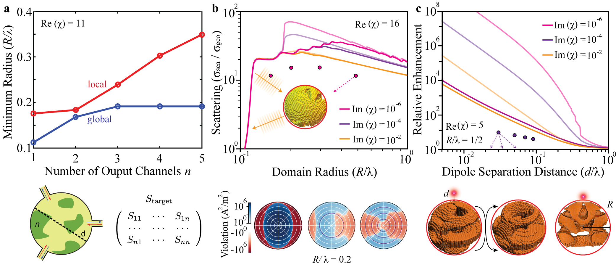
Figure 7: Impact of localized constraints. The figure shows upper bounds under the enforcement of local constraints on a the minimum radius $R$ of a cylindrical design domain necessary to encode a “power-splitting” $\mathbb{S}$ matrix, evenly distributing power from a single plane-wave input into $2n+1$ outgoing radiative channels (Ref. [42]); b plane-wave scattering as described in the previous tutorial (Ref. [41]); and c radiative Purcell enhancement for an electric dipole source in the near field of an object (Ref. [41]). Lighter-colored lines in b and c result from imposing the global conservation of real and reactive power. Like-colored darker lines are obtained by enforcing local conservation constraints over radial shell subdomains (varying distribution with application). As in previous plots, dots in b and c mark actual enhancement values achieved by structures discovered by computational methods. Views of one such design are given below c. The logarithmic color maps included below b indicate the local violation of the conservation of reactive power for $1,2$, and $4$ evenly spaced shell subregion constraints. The schematic shown below a conceptualizes the engineering of a device to realize a particular scattering matrix. In all three panels, additional constraints lead to increasingly realistic field features and limit values.

Owing to the nature of the relaxation techniques commonly used to solve optimization bounds (c.f. Refs. [41, 44]), the spatial oscillation of such local violations of “true” physics tend to track the spatial oscillations of the incident field, as seen in Fig. 7b, and accordingly, by imposing localized projections ($\mathbb{P}=\mathbb{I}_{\mathsf{P}}$ where $\mathsf{P}\subset\Omega$) in Eq. (10) targeting a specific region of violation, it is usually possible to guide optimization limits towards increasingly physical characteristics: the vacuum Green’s function $\mathbb{G}_{0}$ does not propagate all information equally, but rather blurs rapid field fluctuations as the point of observation moves away from the source. As such, for each design problem, there are characteristic lengths below which differences between field solutions have no pragmatic relevance. If independent constraints enforce “averaged” physics on a grid finer than the smallest of these length scales, then the solution of Eq. (13) should differ little from what is realizable in practice [199]. Directly, the number and distribution of local constraints can be viewed as “tuning knobs” enforcing physics at the expense of computational complexity.

An exemplification of these ideas is illustrated by the minimum-radius limits on a two-dimensional power splitter, distributing power from an incident wave equally between $2n+1$ cylindrical wave channels, depicted in Fig. 7a (Ref. [42]). In asserting only the conservation of global power, the minimum diameter asymptotes to $\sim\lambda/3$, a size at which it begins to become possible for a non-physical response oscillating near $\lambda/\sqrt{\real(\chi)+1}$ to satisfy global power conservation while maintaining large local violations. Opposingly, when local constraints are added, this asymptote disappears and the required radius (suggesting increasing device complexity) begins to grow steadily with the number of power divisions desired. In Fig 7b, the strict use of global constraints similarly suggests that shortly after attaining a resonance criteria of $R\gtrsim\lambda/5$, by structuring a material with $\real(\chi)=16$ within a spherical ball of radius $R$, it is possible to enhance the scattering cross section inversely proportional to material loss ($\imaginary(\chi)$). No such scaling is found in computationally synthesized structures, marked in the figure by dots, and under the imposition of $8$ (evenly spaced) radial shell constraints this nonphysical feature all but vanishes.

Stemming from the need to properly describe sub-wavelength field characteristics, local constraints are also generally required to formulate relevant limits on near field phenomena. Following Fig. 7c—bounds on the maximization of radiative Purcell enhancement for a dipolar current source separated from an arbitrary device by a distance $d$, again contained within a spherical ball of radius $R$—when only global constraints are considered enhancement is seen to scale $\propto 1/\imaginary\chi$ when $d\ll\lambda$ (light lines), as is characteristic of material loss limited resonant response [75]. Upon inclusion of localized constraints defined over concentric spherical shells (dark lines), the maximal radiation is observed to drop by several orders of magnitude and no longer grows with decreasing $\imaginary\chi$, confirming the challenge of achieving optimal polarization fields capable of resonantly scattering evanescent fields into propagating waves. Conversely, even with many more localizing shells (see Ref. [41] for details), limits on larger domains and stronger dielectrics show no such saturation and exhibit $\propto d^{-3}$ diverging growth—implying that arbitrarily high angular momentum states can be out-coupled with nearly fixed efficiency. Because of the resolution arguments stated above, if additional non-symmetric localized constraints were to be imposed, particularly in the region of the design volume nearest the dipole, tighter limits may be anticipated.

Figure 8: From performance bounds to structural optimization. Through the common denominator of spatial divisions, a complementary relationship exists between inverse design and performance bounds. In inverse design, the non-convex optimization problem of structural optimization is heuristically approximated by particular designs representing local optima, with resulting device performance generally increasing with additional structural degrees of freedom. In optimization bounds, a coarse grained version of the same optimization problem is bounded by exploiting some convex relaxation in order to determine a value that must be respected by all allowed designs, with resulting limits generally becoming tighter under the use of additional constraints. Consequently, as the number and resolution of the local constraints going into a bounds QCQP is increased, its solution fields typically become increasingly better approximations of the polarization field of a globally optimal structure. This observation suggests a potential, presently unexplored, workflow for the computational design of photonic devices: evaluate the limits of an application to a tightness wherein the approximate field distribution can be extracted and used as a starting point for the discovery of near optimal structures.

Outlook

As exemplified by the preceding discussion and representative examples, the nascent development of a methodology combining physical constraints with optimization theory has already proven to be a remarkably versatile and fruitful framework for understanding and computing electromagnetic limits. Still, a panorama of challenges and opportunities remain. First, the core ideas behind the method are by no means restricted to phenomena governed by Maxwell’s equations, and have direct analogues in other domains of wave physics, such as acoustics and quantum mechanics. And even more broadly, the general concept of obtaining performance limits by rigorously bounding a simpler problem through relaxed physics is applicable to essentially any field of engineering. (See Ref. [153] for recent applications to quantum control.) Second, as it currently stands, the framework requires physical objectives to be formulated as quadratic functions of the polarization fields, which excludes various photonic problems, including nonlinear processes (such as the Kerr effect) or objectives which may be more naturally expressed as eigenproblems (such as the maximization of bandgaps [200] or the engineering of Dirac points [201]. Yet another avenue for further research, particularly relevant to device applications, is the incorporation of fabrication constraints. Presently, the limit framework considers any possible structure that may fit within the design region without regard for existing nanofabrication constraints such as minimum feature sizes and material connectivity.

Moreover, it is not yet understood whether, or under what conditions, the convex relaxation techniques that are used to obtain optimization limits can be guaranteed to solve their associated QCQPs, i.e., whether the limit is equal to the true QCQP solution or just some larger (resp. smaller) value. Non-affine equality constraints such as the conservation of real and reactive power are non-convex, and QCQPs with non-convex constraints are not generally thought to be solvable by any convex relaxation [202, 44]. So far, however, a vast majority of investigations have found that calculated limit fields are in fact optimal solutions of the initial optimization problem statement [39, 38, 41], with inclusion of large numbers of local constraints only resulting in numerical ill-conditioning. Such guarantees are not merely a theoretical exercise. So long as the underlying QCQP is actually solved, through the addition of increasingly finer localized constraints progressively better approximations to an optimal realizable polarization field emerge from bounds computations, and this information could be leveraged to great effect in inverse design. For instance, it could be used as a starting point for adjoint optimization to recover a near optimal structure, see Fig. 8, or as a guide for the design parameters that should be considered to possibly realize improved performance characteristics. Furthermore, it is likely not necessary to enforce local constraints down to the computational pixel level to make use of these potentially powerful connections; a coarse distribution may be enough to extract an approximate optimal structure. Indeed, the onset of ill-conditioning with finer local constraints suggests that, depending on the design problem, there is a characteristic length scale beyond which more detailed structuring becomes unnecessary. Relatedly, while the bounds computation is convex, it is not necessarily easy to solve numerically. Besides ill-conditioning resulting from the imposition of large numbers of local constraints, numerical instabilities also occur in systems with low loss (e.g., semi-transparent media). To address this, it may be possible to formulate alternate constraints better suited to handle low-loss/lossless design problems; one example is given by Ref. [198], though the proposed constraints appear to provide non-trivial limits only for small design regions and low dielectric contrasts.

The large scale of most practical photonics problems also poses a challenge: current demonstrations of the framework are restricted to 2D [198, 42, 44, 43] or highly symmetric domains in 3D, exploiting efficient spectral basis representations [39, 38, 68] to limit the size of the associated system matrices. Beyond these early proof-of-concept explorations, there is much room for development of standardized packages for evaluating limits (possibly in conjunction with inverse methods) on 3D photonic devices by exploiting general-purpose techniques—numerical Maxwell solvers employing localized bases—and open-source optimization methods [203].

References

- Yariv and Yeh [2006] A. Yariv and P. Yeh, Photonics: optical electronics in modern communications (Oxford University Press, Inc., 2006).
- Oh et al. [2021] S.-H. Oh, H. Altug, X. Jin, T. Low, S. J. Koester, A. P. Ivanov, J. B. Edel, P. Avouris, and M. S. Strano, Nanophotonic biosensors harnessing van der Waals materials, Nature Communications 12, 10.1038/s41467-021-23564-4 (2021).
- Zhang et al. [2021a] S. Zhang, C. L. Wong, S. Zeng, R. Bi, K. Tai, K. Dholakia, and M. Olivo, Metasurfaces for biomedical applications: imaging and sensing from a nanophotonics perspective, Nanophotonics 10, 10.1515/nanoph-2020-0373 (2021a).
- Garnett et al. [2020] E. C. Garnett, B. Ehrler, A. Polman, and E. Alarcon-Llado, Photonics for photovoltaics: advances and opportunities, ACS Photonics 8, 61 (2020).
- Brunner et al. [2020] D. Brunner, A. Marandi, W. Bogaerts, and A. Ozcan, Photonics for computing and computing for photonics, Nanophotonics 9, 4053 (2020).
- Shastri et al. [2021] B. J. Shastri, A. N. Tait, T. Ferreira de Lima, W. H. P. Pernice, H. Bhaskaran, C. D. Wright, and P. R. Prucnal, Photonics for artificial intelligence and neuromorphic computing, Nature Photonics 15, 10.1038/s41566-020-00754-y (2021).
- Dory et al. [2019] C. Dory, D. Vercruysse, K. Y. Yang, N. V. Sapra, A. E. Rugar, S. Sun, D. M. Lukin, A. Y. Piggott, J. L. Zhang, M. Radulaski, et al., Inverse-designed diamond photonics, Nature communications 10, 1 (2019).
- Chakravarthi et al. [2020] S. Chakravarthi, P. Chao, C. Pederson, S. Molesky, A. Ivanov, K. Hestroffer, F. Hatami, A. W. Rodriguez, and K.-M. C. Fu, Inverse-designed photon extractors for optically addressable defect qubits, Optica 7, 1805 (2020).
- Liu et al. [2016] K. Liu, S. Sun, A. Majumdar, and V. J. Sorger, Fundamental scaling laws in nanophotonics, Scientific Reports 6, 37419 (2016).
- Joannopoulos et al. [2008] J. D. Joannopoulos, S. G. Johnson, J. N. Winn, and R. D. Meade, Photonic crystals: molding the flow of light (Princeton University Press, 2008).
- Vahala [2003] K. J. Vahala, Optical microcavities, Nature 424, 839 (2003).
- Khurgin [2015] J. B. Khurgin, How to deal with the loss in plasmonics and metamaterials, Nature Nanotechnology 10, 2 (2015).
- Jacob et al. [2010] Z. Jacob, J.-Y. Kim, G. V. Naik, A. Boltasseva, E. E. Narimanov, and V. M. Shalaev, Engineering photonic density of states using metamaterials, Applied physics B 100, 215 (2010).
- Sreekanth et al. [2014] K. V. Sreekanth, K. H. Krishna, A. De Luca, and G. Strangi, Large spontaneous emission rate enhancement in grating coupled hyperbolic metamaterials, Scientific Reports 4, 1 (2014).
- Popov et al. [2016] V. Popov, A. V. Lavrinenko, and A. Novitsky, Operator approach to effective medium theory to overcome a breakdown of maxwell garnett approximation, Physical Review B 94, 085428 (2016).
- Schneider et al. [2019] P.-I. Schneider, X. Garcia Santiago, V. Soltwisch, M. Hammerschmidt, S. Burger, and C. Rockstuhl, Benchmarking five global optimization approaches for nano-optical shape optimization and parameter reconstruction, ACS Photonics 6, 2726 (2019).
- Lalau-Keraly et al. [2013] C. M. Lalau-Keraly, S. Bhargava, O. D. Miller, and E. Yablonovitch, Adjoint shape optimization applied to electromagnetic design, Optics Express 21, 21693 (2013).
- Liang and Johnson [2013] X. Liang and S. G. Johnson, Formulation for scalable optimization of microcavities via the frequency-averaged local density of states, Optics Express 21, 30812 (2013).
- Christiansen and Sigmund [2021] R. E. Christiansen and O. Sigmund, Inverse design in photonics by topology optimization: tutorial, JOSA B 38, 496 (2021).
- Liu et al. [2018a] D. Liu, Y. Tan, E. Khoram, and Z. Yu, Training deep neural networks for the inverse design of nanophotonic structures, ACS Photonics 5, 1365 (2018a).
- Jiang et al. [2021] J. Jiang, M. Chen, and J. A. Fan, Deep neural networks for the evaluation and design of photonic devices, Nature Reviews Materials 6, 10.1038/s41578-020-00260-1 (2021).
- Note [1] Inverse methods may converge to structures that appear to reflect intuitive design principles, such as bowtie antenna and slot waveguide motifs for enhancing light-matter interaction [18, 204, 34].
- Betzig et al. [1986] E. Betzig, A. Lewis, A. Harootunian, M. Isaacson, and E. Kratschmer, Near field scanning optical microscopy (nsom): development and biophysical applications, Biophysical Journal 49, 269 (1986).
- Sánchez et al. [1999] E. J. Sánchez, L. Novotny, and X. S. Xie, Near-field fluorescence microscopy based on two-photon excitation with metal tips, Physical Review Letters 82, 4014 (1999).
- Pendry [2000] J. B. Pendry, Negative refraction makes a perfect lens, Physical Review Letters 85, 3966 (2000).
- Vicidomini et al. [2018] G. Vicidomini, P. Bianchini, and A. Diaspro, STED super-resolved microscopy, Nature Methods 15, 10.1038/nmeth.4593 (2018).
- Bates et al. [2013] M. Bates, S. A. Jones, and X. Zhuang, Stochastic optical reconstruction microscopy (storm): a method for superresolution fluorescence imaging, Cold Spring Harbor Protocols 2013, 10.1101/pdb.top075143 (2013).
- Shockley and Queisser [1961] W. Shockley and H. J. Queisser, Detailed balance limit of efficiency of p-n junction solar cells, Journal of Applied Physics 32, 510 (1961).
- López and Andreev [2007] A. L. López and V. M. Andreev, Concentrator photovoltaics, Vol. 130 (Springer, 2007).
- Henry [1980] C. H. Henry, Limiting efficiencies of ideal single and multiple energy gap terrestrial solar cells, Journal of Applied Physics 51, 4494 (1980).
- Luque and Martí [1997] A. Luque and A. Martí, Increasing the efficiency of ideal solar cells by photon induced transitions at intermediate levels, Physical Review Letters 78, 5014 (1997).
- Guo et al. [2012] Y. Guo, C. L. Cortes, S. Molesky, and Z. Jacob, Broadband super-Planckian thermal emission from hyperbolic metamaterials, Applied Physics Letters 101, 131106 (2012).
- Thompson et al. [2018] D. Thompson, L. Zhu, R. Mittapally, S. Sadat, Z. Xing, P. McArdle, M. M. Qazilbash, P. Reddy, and E. Meyhofer, Hundred-fold enhancement in far-field radiative heat transfer over the blackbody limit, Nature 561, 216 (2018).
- Albrechtsen et al. [2021] M. Albrechtsen, B. V. Lahijani, R. E. Christiansen, V. T. H. Nguyen, L. N. Casses, S. E. Hansen, N. Stenger, O. Sigmund, H. Jansen, J. Mørk, et al., Nanometer-scale photon confinement inside dielectrics, arXiv:2108.01681 (2021).
- Kudyshev et al. [2020] Z. A. Kudyshev, A. V. Kildishev, V. M. Shalaev, and A. Boltasseva, Machine-learning-assisted metasurface design for high-efficiency thermal emitter optimization, Applied Physics Reviews 7, 021407 (2020).
- Christiansen et al. [2020] R. E. Christiansen, Z. Lin, C. Roques-Carmes, Y. Salamin, S. E. Kooi, J. D. Joannopoulos, M. Soljačić, and S. G. Johnson, Fullwave Maxwell inverse design of axisymmetric, tunable, and multi-scale multi-wavelength metalenses, Optics Express 28, 33854 (2020).
- Phan et al. [2019] T. Phan, D. Sell, E. W. Wang, S. Doshay, K. Edee, J. Yang, and J. A. Fan, High-efficiency, large-area, topology-optimized metasurfaces, Light: Science & Applications 8, 1 (2019).
- Molesky et al. [2020a] S. Molesky, P. S. Venkataram, W. Jin, and A. W. Rodriguez, Fundamental limits to radiative heat transfer: theory, Physical Review B 101, 035408 (2020a).
- Gustafsson et al. [2020] M. Gustafsson, K. Schab, L. Jelinek, and M. Capek, Upper bounds on absorption and scattering, New Journal of Physics 22, 073013 (2020).
- Kuang et al. [2020] Z. Kuang, L. Zhang, and O. D. Miller, Maximal single-frequency electromagnetic response, Optica 7, 1746 (2020).
- Molesky et al. [2020b] S. Molesky, P. Chao, and A. W. Rodriguez, Hierarchical mean-field operator bounds on electromagnetic scattering: Upper bounds on near-field radiative purcell enhancement, Physical Review Research 2, 043398 (2020b).
- Kuang and Miller [2020] Z. Kuang and O. D. Miller, Computational bounds to light–matter interactions via local conservation laws, Physical Review Letters 125, 263607 (2020).
- Molesky et al. [2021] S. Molesky, P. Chao, J. Mohajan, W. Reinhart, H. Chi, and A. W. Rodriguez, -operator limits on optical communication: Metaoptics, computation, and input-output transformations, (2021), arXiv:2102.10175 [physics.optics] .
- Angeris et al. [2021a] G. Angeris, J. Vučković, and S. Boyd, Heuristic methods and performance bounds for photonic design, Optics Express 29, 2827 (2021a).
- Brillouin [2013] L. Brillouin, Wave propagation and group velocity, Vol. 8 (Academic press, 2013).
- Schulz-DuBois [1969] E. Schulz-DuBois, Energy transport velocity of electromagnetic propagation in dispersive media, Proceedings of the IEEE 57, 1748 (1969).
- Loudon [1970] R. Loudon, The propagation of electromagnetic energy through an absorbing dielectric, Journal of Physics A: General Physics 3, 233 (1970).
- Yaghjian [2007] A. D. Yaghjian, Internal energy, Q-energy, Poynting’s theorem, and the stress dyadic in dispersive material, IEEE Transactions on Antennas and Propagation 55, 1495 (2007).
- Glasgow et al. [2001] S. Glasgow, M. Ware, and J. Peatross, Poynting’s theorem and luminal total energy transport in passive dielectric media, Physical Review E 64, 046610 (2001).
- Welters et al. [2014] A. Welters, Y. Avniel, and S. G. Johnson, Speed-of-light limitations in passive linear media, Physical Review A 90, 023847 (2014).
- Tucker et al. [2005] R. Tucker, Pei-Cheng Ku, and C. Chang-Hasnain, Slow-light optical buffers: capabilities and fundamental limitations, Journal of Lightwave Technology 23, 4046 (2005).
- Liu et al. [2001] C. Liu, Z. Dutton, C. H. Behroozi, and L. V. Hau, Observation of coherent optical information storage in an atomic medium using halted light pulses, Nature 409, 490 (2001).
- Hau et al. [1999] L. V. Hau, S. E. Harris, Z. Dutton, and C. H. Behroozi, Light speed reduction to 17 metres per second in an ultracold atomic gas, Nature 397, 594 (1999).
- Yariv et al. [1999] A. Yariv, Y. Xu, R. K. Lee, and A. Scherer, Coupled-resonator optical waveguide: a proposal and analysis, Optics Letters 24, 711 (1999).
- Soljačić et al. [2002] M. Soljačić, S. G. Johnson, S. Fan, M. Ibanescu, E. Ippen, and J. D. Joannopoulos, Photonic-crystal slow-light enhancement of nonlinear phase sensitivity, Journal of the Optical Society of America B 19, 2052 (2002).
- Povinelli et al. [2005] M. L. Povinelli, S. G. Johnson, and J. D. Joannopoulos, Slow-light, band-edge waveguides for tunable time delays, Optics Express 13, 7145 (2005).
- Miller [2007a] D. A. B. Miller, Fundamental limit for optical components, Journal of the Optical Society of America B 24, A1 (2007a).
- Miller [2007b] D. A. B. Miller, Fundamental Limit to Linear One-Dimensional Slow Light Structures, Physical Review Letters 99, 203903 (2007b).
- Fleury et al. [2015] R. Fleury, F. Monticone, and A. Alù, Invisibility and cloaking: origins, present, and future perspectives, Physical Review Applied 4, 037001 (2015).
- Pendry [2006] J. B. Pendry, Controlling electromagnetic fields, Science 312, 1780 (2006).
- Hashemi et al. [2011] H. Hashemi, A. Oskooi, J. D. Joannopoulos, and S. G. Johnson, General scaling limitations of ground-plane and isolated-object cloaks, Physical Review A 84, 023815 (2011).
- Chu [1948] L. J. Chu, Physical limitations of omni-directional antennas, Journal of Applied Physics 19, 1163 (1948).
- Yablonovitch [1982] E. Yablonovitch, Statistical ray optics, Journal of the Optical Society of America 72, 899 (1982).
- Fleury et al. [2014] R. Fleury, J. Soric, and A. Alù, Physical bounds on absorption and scattering for cloaked sensors, Physical Review B 89, 045122 (2014).
- Miller [2000] D. A. B. Miller, Communicating with waves between volumes: evaluating orthogonal spatial channels and limits on coupling strengths, Applied Optics 39, 1681 (2000).
- Miller et al. [2017] D. A. Miller, L. Zhu, and S. Fan, Universal modal radiation laws for all thermal emitters, Proceedings of the National Academy of Sciences 114, 4336 (2017).
- Angeris et al. [2019] G. Angeris, J. Vučković, and S. P. Boyd, Computational bounds for photonic design, ACS Photonics 6, 1232 (2019).
- Jelinek et al. [2021] L. Jelinek, M. Gustafsson, M. Capek, and K. Schab, Fundamental bounds on the performance of monochromatic passive cloaks, Optics Express 29, 24068 (2021).
- Maier [2007] S. A. Maier, Plasmonics: fundamentals and applications (Springer Science & Business Media, 2007).
- Lee et al. [2008] K. K. Lee, Y. Avniel, and S. G. Johnson, Rigorous sufficient conditions for index-guided modes in microstructured dielectric waveguides, Optics Express 16, 9261 (2008).
- Rechtsman and Torquato [2009] M. C. Rechtsman and S. Torquato, Method for obtaining upper bounds on photonic band gaps, Physical Review B 80, 155126 (2009).
- Vardeny et al. [2013] Z. V. Vardeny, A. Nahata, and A. Agrawal, Optics of photonic quasicrystals, Nature Photonics 7, 177 (2013).
- Yu et al. [2021] S. Yu, C.-W. Qiu, Y. Chong, S. Torquato, and N. Park, Engineered disorder in photonics, Nature Reviews Materials 6, 226 (2021).
- Pick et al. [2017] A. Pick, B. Zhen, O. D. Miller, C. W. Hsu, F. Hernandez, A. W. Rodriguez, M. Soljačić, and S. G. Johnson, General theory of spontaneous emission near exceptional points, Optics Express 25, 12325 (2017).
- Miller et al. [2016] O. D. Miller, A. G. Polimeridis, M. T. H. Reid, C. W. Hsu, B. G. DeLacy, J. D. Joannopoulos, M. Soljačić, and S. G. Johnson, Fundamental limits to optical response in absorptive systems, Optics Express 24, 3329 (2016).
- Barnett and Loudon [1996] S. M. Barnett and R. Loudon, Sum rule for modified spontaneous emission rates, Physical Review Letters 77, 2444 (1996).
- Scheel [2008] S. Scheel, Sum rule for local densities of states in absorbing dielectrics, Physical Review A 78, 013841 (2008).
- Kuzyk [2000] M. G. Kuzyk, Physical limits on electronic nonlinear molecular susceptibilities, Physical Review Letters 85, 1218 (2000).
- Kuzyk et al. [2013] M. G. Kuzyk, J. Pérez-Moreno, and S. Shafei, Sum rules and scaling in nonlinear optics, Physics Reports Sum Rules and Scaling in Nonlinear Optics, 529, 297 (2013).
- Markvart [2007] T. Markvart, The thermodynamics of optical étendue, Journal of Optics A: Pure and Applied Optics 10, 015008 (2007).
- Ries [1982] H. Ries, Thermodynamic limitations of the concentration of electromagnetic radiation, JOSA 72, 380 (1982).
- Zhang et al. [2019] H. Zhang, C. W. Hsu, and O. D. Miller, Scattering concentration bounds: brightness theorems for waves, Optica 6, 1321 (2019).
- Chung and Miller [2020] H. Chung and O. D. Miller, High-na achromatic metalenses by inverse design, Optics Express 28, 6945 (2020).
- Banerji et al. [2019] S. Banerji, M. Meem, A. Majumder, F. G. Vasquez, B. Sensale-Rodriguez, and R. Menon, Imaging with flat optics: metalenses or diffractive lenses?, Optica 6, 805 (2019).
- Chen et al. [2018] W. T. Chen, A. Y. Zhu, V. Sanjeev, M. Khorasaninejad, Z. Shi, E. Lee, and F. Capasso, A broadband achromatic metalens for focusing and imaging in the visible, Nature Nanotechnology 13, 10.1038/s41565-017-0034-6 (2018).
- Lin and Johnson [2019] Z. Lin and S. G. Johnson, Overlapping domains for topology optimization of large-area metasurfaces, Optics Express 27, 32445 (2019).
- Shrestha et al. [2018] S. Shrestha, A. C. Overvig, M. Lu, A. Stein, and N. Yu, Broadband achromatic dielectric metalenses, Light: Science & Applications 7, 10.1038/s41377-018-0078-x (2018).
- Wang et al. [2018a] S. Wang, P. C. Wu, V.-C. Su, Y.-C. Lai, M.-K. Chen, H. Y. Kuo, B. H. Chen, Y. H. Chen, T.-T. Huang, J.-H. Wang, R.-M. Lin, C.-H. Kuan, T. Li, Z. Wang, S. Zhu, and D. P. Tsai, A broadband achromatic metalens in the visible, Nature Nanotechnology 13, 227 (2018a).
- Presutti and Monticone [2020] F. Presutti and F. Monticone, Focusing on bandwidth: achromatic metalens limits, Optica 7, 624 (2020).
- Kirchhoff [1978] G. Kirchhoff, Über das verhältnis zwischen dem emissionsvermögen und dem absorptionsvermögen der körper für wärme und licht, in Von Kirchhoff bis Planck (Springer, 1978) pp. 131–151.
- Onnes and Ehrenfest [1914] H. K. Onnes and P. Ehrenfest, Simplyfied deduction of the formula from the theory of combinations which Planck uses as the basis of his radiation-theory, in KNAW, Proceedings, Vol. 17 (1914) pp. 870–873.
- Robitaille [2009] P.-M. Robitaille, Kirchhoff’s law of thermal emission: 150 years, Progress in Physics 4, 3 (2009).
- Ellis et al. [2017] A. Ellis, M. McCarthy, M. Al Khateeb, M. Sorokina, and N. Doran, Performance limits in optical communications due to fiber nonlinearity, Advances in Optics and Photonics 9, 429 (2017).
- Mizuno et al. [2009] K. Mizuno, J. Ishii, H. Kishida, Y. Hayamizu, S. Yasuda, D. N. Futaba, M. Yumura, and K. Hata, A black body absorber from vertically aligned single-walled carbon nanotubes, Proceedings of the National Academy of Sciences 106, 6044 (2009).
- Yoon et al. [2015] J. Yoon, M. Zhou, M. A. Badsha, T. Y. Kim, Y. C. Jun, and C. K. Hwangbo, Broadband epsilon-near-zero perfect absorption in the near-infrared, Scientific Reports 5, 1 (2015).
- Magdi et al. [2017] S. Magdi, D. Ji, Q. Gan, and M. A. Swillam, Broadband absorption enhancement in organic solar cells using refractory plasmonic ceramics, Journal of Nanophotonics 11, 016001 (2017).
- Venkataram et al. [2020a] P. S. Venkataram, S. Molesky, W. Jin, and A. W. Rodriguez, Fundamental limits to radiative heat transfer: the limited role of nanostructuring in the near-field, Physical Review Letters 124, 013904 (2020a).
- Yu et al. [2010] Z. Yu, A. Raman, and S. Fan, Fundamental limit of nanophotonic light trapping in solar cells, Proceedings of the National Academy of Sciences 107, 17491 (2010).
- Dienerowitz et al. [2008] M. Dienerowitz, M. Mazilu, and K. Dholakia, Optical manipulation of nanoparticles: a review, Journal of Nanophotonics 2, 021875 (2008).
- Macchi et al. [2009] A. Macchi, S. Veghini, and F. Pegoraro, Light sail acceleration reexamined, Physical Review Letters 103, 085003 (2009).
- Kenneth and Klich [2006] O. Kenneth and I. Klich, Opposites attract: a theorem about the Casimir force, Physical Review Letters 97, 160401 (2006).
- Venkataram et al. [2020b] P. S. Venkataram, S. Molesky, P. Chao, and A. W. Rodriguez, Fundamental limits to attractive and repulsive casimir-polder forces, Physical Review A 101, 052115 (2020b).
- Gustafsson and Nordebo [2013] M. Gustafsson and S. Nordebo, Optimal antenna currents for Q, superdirectivity, and radiation patterns using convex optimization, IEEE Transactions on Antennas and Propagation 61, 1109 (2013).
- Gustafsson and Capek [2019] M. Gustafsson and M. Capek, Maximum gain, effective area, and directivity, IEEE Transactions on Antennas and Propagation 67, 5282 (2019).
- Capek et al. [2017] M. Capek, M. Gustafsson, and K. Schab, Minimization of antenna quality factor, IEEE Transactions on Antennas and Propagation 65, 10.1109/TAP.2017.2717478 (2017).
- Capek et al. [2019] M. Capek, L. Jelinek, K. Schab, M. Gustafsson, B. L. G. Jonsson, F. Ferrero, and C. Ehrenborg, Optimal planar electric dipole antennas: searching for antennas reaching the fundamental bounds on selected metrics, IEEE Antennas and Propagation Magazine 61, 19 (2019).
- Boyd and Vandenberghe [2004] S. Boyd and L. Vandenberghe, Convex optimization (Cambridge University Press, 2004).
- Zhao et al. [2020] Q. Zhao, L. Zhang, and O. D. Miller, Minimum dielectric-resonator mode volumes, arXiv:2008.13241 (2020).
- Bérenger [2007] J.-P. Bérenger, On the Huygens absorbing boundary conditions for electromagnetics, Journal of Computational Physics 226, 354 (2007).
- Lindell and Sihvola [2019] I. V. Lindell and A. Sihvola, Boundary conditions in electromagnetics (John Wiley & Sons, 2019).
- Molesky et al. [2020c] S. Molesky, P. Chao, W. Jin, and A. W. Rodriguez, Global operator bounds on electromagnetic scattering: upper bounds on far-field cross sections, Physical Review Research 2, 033172 (2020c).
- Sun and Chew [2009] L. Sun and W. C. Chew, A novel formulation of the volume integral equation for electromagnetic scattering, Waves in Random and Complex Media 19, 162 (2009).
- Samokhin [2013] A. B. Samokhin, Integral equations and iteration methods in electromagnetic scattering (de Gruyter, 2013).
- Costabel et al. [2012] M. Costabel, E. Darrigrand, and H. Sakly, The essential spectrum of the volume integral operator in electromagnetic scattering by a homogeneous body, (2012).
- Polimeridis et al. [2014] A. G. Polimeridis, M. T. H. Reid, S. G. Johnson, J. K. White, and A. W. Rodriguez, On the computation of power in volume integral equation formulations, IEEE Transactions on Antennas and Propagation 63, 611 (2014).
- Polimeridis et al. [2015] A. G. Polimeridis, M. T. H. Reid, W. Jin, S. G. Johnson, J. K. White, and A. W. Rodriguez, Fluctuating volume-current formulation of electromagnetic fluctuations in inhomogeneous media: Incandescence and luminescence in arbitrary geometries, Physical Review B 92, 134202 (2015).
- Liu et al. [2018b] Q. S. Liu, S. Sun, and W. C. Chew, A potential-based integral equation method for low-frequency electromagnetic problems, IEEE Transactions on Antennas and Propagation 66, 1413 (2018b).
- Lippmann and Schwinger [1950] B. A. Lippmann and J. Schwinger, Variational principles for scattering processes, Physical Review 79, 469 (1950).
- Lanczos [1950] C. Lanczos, An iteration method for the solution of the eigenvalue problem of linear differential and integral operators, (1950).
- Tsang et al. [2004] L. Tsang, J. A. Kong, and K.-H. Ding, Scattering of electromagnetic waves: theories and applications, Vol. 27 (John Wiley & Sons, 2004).
- Note [2] It is equally possible to derive results completely analogous to Eqs. (5\@@italiccorr)–(8\@@italiccorr) using scattered electromagnetic fields [44], as opposed to the polarization current density perspective used here.
- Note [3] The Green’s function (fundamental solution) of a linear differential equation is the solution of the differential equations for the Dirac distribution, i.e. in our notation. The solution of the differential equation for any inhomogeneous source term is given by convolution with the Green’s function [123].
- Novotny and Hecht [2012] L. Novotny and B. Hecht, Principles of nano-optics (Cambridge university press, 2012).
- Kanwal [2013] R. P. Kanwal, Linear integral equations (Springer Science & Business Media, 2013).
- Krüger et al. [2012] M. Krüger, G. Bimonte, T. Emig, and M. Kardar, Trace formulas for nonequilibrium casimir interactions, heat radiation, and heat transfer for arbitrary objects, Physical Review B 86, 115423 (2012).
- Dyson [1949] F. J. Dyson, The s matrix in quantum electrodynamics, Physical Review 75, 1736 (1949).
- Gell-Mann and Goldberger [1953] M. Gell-Mann and M. Goldberger, The formal theory of scattering, Physical Review 91, 398 (1953).
- Van Kampen [1953] N. Van Kampen, S-matrix and causality condition. I. Maxwell field, Physical Review 89, 1072 (1953).
- Landau and Lifshitz [2013a] L. D. Landau and E. M. Lifshitz, Statistical physics: volume 5, Vol. 5 (Elsevier, 2013).
- Rudin [1991] W. Rudin, Functional analysis (McGraw-Hill Education, New York, 1991).
- Note [4] The same conclusion, with minor modifications, also holds if the design domain is split into a collection of subdomains, and in each subdomain any possible structuring must be carried out in a single known material.
- Rudin [2006] W. Rudin, Real and complex analysis (McGraw-Hill Education, New York, 2006).
- Note [5] Technically, the integral is an inner product for almost everywhere equal equivalences classes of functions and fields. However, because we are primarily concerned with finite numerical representations, here the distinction is not important.
- Note [6] Given our freedom in choosing there is no difference between and .
- Miller et al. [2014] O. D. Miller, C. W. Hsu, M. T. H. Reid, W. Qiu, B. G. DeLacy, J. D. Joannopoulos, M. Soljačić, and S. G. Johnson, Fundamental limits to extinction by metallic nanoparticles, Physical Review Letters 112, 123903 (2014).
- Molesky et al. [2019] S. Molesky, W. Jin, P. S. Venkataram, and A. W. Rodriguez, -operator bounds on angle-integrated absorption and thermal radiation for arbitrary objects, Physical Review Letters 123, 257401 (2019).
- Jackson [1999] J. D. Jackson, Classical electrodynamics (AAPT, 1999).
- Vercruysse et al. [2014] D. Vercruysse, X. Zheng, Y. Sonnefraud, N. Verellen, G. Di Martino, L. Lagae, G. A. Vandenbosch, V. V. Moshchalkov, S. A. Maier, and P. Van Dorpe, Directional fluorescence emission by individual v-antennas explained by mode expansion, ACS Nano 8, 8232 (2014).
- Shahpari and Thiel [2018] M. Shahpari and D. V. Thiel, Fundamental limitations for antenna radiation efficiency, IEEE Transactions on Antennas and Propagation 66, 3894 (2018).
- Siegel and Spuckler [1993] R. Siegel and C. M. Spuckler, Refractive index effects on radiation in an absorbing, emitting, and scattering laminated layer, Journal of Heat Transfer 115, 194 (1993).
- Yu et al. [2012] Z. Yu, A. Raman, and S. Fan, Thermodynamic upper bound on broadband light coupling with photonic structures, Physical Review Letters 109, 173901 (2012).
- Callahan et al. [2012] D. M. Callahan, J. N. Munday, and H. A. Atwater, Solar cell light trapping beyond the ray optic limit, Nano letters 12, 214 (2012).
- Mokkapati and Catchpole [2012] S. Mokkapati and K. Catchpole, Nanophotonic light trapping in solar cells, Journal of Applied Physics 112, 101101 (2012).
- Miroshnichenko and Tribelsky [2018] A. E. Miroshnichenko and M. I. Tribelsky, Ultimate absorption in light scattering by a finite obstacle, Physical Review Letters 120, 033902 (2018).
- Niv et al. [2012] A. Niv, M. Gharghi, C. Gladden, O. D. Miller, and X. Zhang, Near-field electromagnetic theory for thin solar cells, Physical Review Letters 109, 138701 (2012).
- Miller and Yablonovitch [2013] O. D. Miller and E. Yablonovitch, Photon extraction: the key physics for approaching solar cell efficiency limits, in Active Photonic Materials V, Vol. 8808 (International Society for Optics and Photonics, 2013) p. 880807.
- Xu et al. [2015] Y. Xu, T. Gong, and J. N. Munday, The generalized Shockley-Queisser limit for nanostructured solar cells, Scientific Reports 5, 13536 (2015).
- Note [7] Practically, the size of K in numeric simulation is set by the size of the fields.
- Note [8] A feasible field is a field that respects every imposed constraint. The feasible set of an optimization statement is the collection of all feasible fields.
- Schab et al. [2020] K. Schab, A. Rothschild, K. Nguyen, M. Capek, L. Jelinek, and M. Gustafsson, Trade-offs in absorption and scattering by nanophotonic structures, Optics Express 28, 36584 (2020).
- Capek et al. [2021] M. Capek, L. Jelinek, and M. Masek, Fundamental bounds for multi-port antennas, in 2021 15th European Conference on Antennas and Propagation (EuCAP) (IEEE, 2021) pp. 1–4.
- Shim et al. [2019] H. Shim, L. Fan, S. G. Johnson, and O. D. Miller, Fundamental limits to near-field optical response over any bandwidth, Physical Review X 9, 011043 (2019).
- Zhang et al. [2021b] H. Zhang, Z. Kuang, S. Puri, and O. D. Miller, Conservation-law-based global bounds to quantum optimal control, (2021b), 2105.06054 .
- Li et al. [2017] J. Li, F. Ren, T. Hu, Z. Li, Y. He, Z. Chen, Q. Mo, and G. Li, Recent progress in mode-division multiplexed passive optical networks with low modal crosstalk, Optical Fiber Technology 35, 28 (2017).
- Yang et al. [2020] Z. Yang, X. Zhang, B. Zhang, X. Zhang, Z. Zhang, X. Meng, and C. Bai, Density-matrix formalism for modal coupling and dispersion in mode-division multiplexing communications systems, Optics Express 28, 18658 (2020).
- Feng et al. [2020] C. Feng, Z. Ying, Z. Zhao, J. Gu, D. Z. Pan, and R. T. Chen, Wavelength-division-multiplexing (wdm)-based integrated electronic–photonic switching network (epsn) for high-speed data processing and transportation, Nanophotonics 9, 4579 (2020).
- Staude et al. [2019] I. Staude, T. Pertsch, and Y. S. Kivshar, All-dielectric resonant meta-optics lightens up, ACS Photonics 6, 802 (2019).
- Lin et al. [2020] Z. Lin, C. Roques-Carmes, R. Pestourie, M. Soljačić, A. Majumdar, and S. G. Johnson, End-to-end inverse fesign for inverse scattering via freeform metastructures, arXiv:2006.09145 (2020).
- Estakhri et al. [2019] N. M. Estakhri, B. Edwards, and N. Engheta, Inverse-designed metastructures that solve equations, Science 363, 1333 (2019).
- Li et al. [2019] L. Li, Y. Shuang, Q. Ma, H. Li, H. Zhao, M. Wei, C. Liu, C. Hao, C.-W. Qiu, and T. J. Cui, Intelligent metasurface imager and recognizer, Light: Science & Applications 8, 1 (2019).
- Rajabalipanah et al. [2020] H. Rajabalipanah, A. Abdolali, S. Iqbal, L. Zhang, and T. J. Cui, How do space-time digital metasurfaces serve to perform analog signal processing?, arXiv:2002.06773 (2020).
- Kravtsov et al. [1975] Y. A. Kravtsov, S. Rytov, and V. Tatarskiĭ, Statistical problems in diffraction theory, Soviet Physics Uspekhi 18, 118 (1975).
- Rytov et al. [1988] S. M. Rytov, Y. A. Kravtsov, and V. I. Tatarskii, Principles of statistical radiophysics 2. correlation theory of random processes. (1988).
- Kubo [1966] R. Kubo, The fluctuation-dissipation theorem, Reports on Progress in Physics 29, 255 (1966).
- Mörters and Peres [2010] P. Mörters and Y. Peres, Brownian motion, Vol. 30 (Cambridge University Press, 2010).
- Marconi et al. [2008] U. M. B. Marconi, A. Puglisi, L. Rondoni, and A. Vulpiani, Fluctuation–dissipation: response theory in statistical physics, Physics Reports 461, 111 (2008).
- Landauer [1989] R. Landauer, Johnson-Nyquist noise derived from quantum mechanical transmission, Physica D: Nonlinear Phenomena 38, 226 (1989).
- Gustafsson et al. [2007] M. Gustafsson, C. Sohl, and G. Kristensson, Physical limitations on antennas of arbitrary shape, Proceedings of the Royal Society A: Mathematical, Physical and Engineering Sciences 463, 2589 (2007).
- Hamilton and Courtial [2009] A. C. Hamilton and J. Courtial, Metamaterials for light rays: ray optics without wave-optical analog in the ray-optics limit, New Journal of Physics 11, 013042 (2009).
- Note [9] The convention used here is .
- Bimonte et al. [2017] G. Bimonte, T. Emig, M. Kardar, and M. Krüger, Nonequilibrium fluctuational quantum electrodynamics: Heat radiation, heat transfer, and force, Annual Review of Condensed Matter Physics 8, 119 (2017), https://doi.org/10.1146/annurev-conmatphys-031016-025203 .
- Note [10] Up to a constant, is the polarization current resulting from the -th radiative mode.
- Miller et al. [2015] O. D. Miller, S. G. Johnson, and A. W. Rodriguez, Shape-independent limits to near-field radiative heat transfer, Physical Review Letters 115, 204302 (2015).
- Xu et al. [2019] H. J. Xu, Z. B. Xing, F. Wang, and Z. Cheng, Review on heat conduction, heat convection, thermal radiation and phase change heat transfer of nanofluids in porous media: Fundamentals and applications, Chemical Engineering Science 195, 462 (2019).
- Beck and Eldar [2006] A. Beck and Y. C. Eldar, Strong duality in nonconvex quadratic optimization with two quadratic constraints, SIAM Journal on Optimization 17, 844 (2006).
- Gustafsson et al. [2019] M. Gustafsson, M. Capek, and K. Schab, Tradeoff between antenna efficiency and Q-factor, IEEE Transactions on Antennas and Propagation 67, 2482 (2019).
- Harrington [1960] R. F. Harrington, Effect of antenna size on gain, bandwidth, and efficiency, Journal of Research of the National Bureau of Standards, Section D: Radio Propagation 64D, 1 (1960).
- McLean [1996] J. S. McLean, A re-examination of the fundamental limits on the radiation Q of electrically small antennas, IEEE Transactions on Antennas and Propagation 44, 672 (1996).
- Capek and Jelinek [2016] M. Capek and L. Jelinek, Optimal composition of modal currents for minimal quality factor Q, IEEE Transactions on Antennas and Propagation 64, 5230 (2016).
- Note [11] Similar limit tightening also occurs when the conservation of reactive power is enforced for thermal radiation as applied to dielectric materials and subwavelength design domains.
- Note [12] Here, by resonant response, we mean that, under sufficiently small changes to the material properties of a design, there is a field observable that scales roughly as .
- Hamam et al. [2007] R. E. Hamam, A. Karalis, J. D. Joannopoulos, and M. Soljačić, Coupled-mode theory for general free-space resonant scattering of waves, Physical Review A 75, 053801 (2007).
- Landau and Lifshitz [2013b] L. D. Landau and E. M. Lifshitz, Quantum mechanics: non-relativistic theory, Vol. 3 (Elsevier, 2013).
- Haus and Huang [1991] H. Haus and W. Huang, Coupled-mode theory, Proceedings of the IEEE 79, 1505 (1991).
- Geyi [2003] W. Geyi, Physical limitations of antenna, IEEE Transactions on Antennas and Propagation 51, 2116 (2003).
- Kwon and Pozar [2009] D.-H. Kwon and D. M. Pozar, Optimal characteristics of an arbitrary receive antenna, IEEE Transactions on Antennas and Propagation 57, 3720 (2009).
- Verslegers et al. [2010] L. Verslegers, Z. Yu, P. B. Catrysse, and S. Fan, Temporal coupled-mode theory for resonant apertures, Journal of the Optical Society of America B 27, 1947 (2010).
- Ruan and Fan [2012] Z. Ruan and S. Fan, Temporal coupled-mode theory for light scattering by an arbitrarily shaped object supporting a single resonance, Physical Review A 85, 043828 (2012).
- Munday et al. [2012] J. N. Munday, D. M. Callahan, and H. A. Atwater, Light trapping beyond the limit in thin waveguides, Applied Physics Letters 100, 121121 (2012).
- Liberal et al. [2014] I. Liberal, I. Ederra, R. Gonzalo, and R. W. Ziolkowski, Upper bounds on scattering processes and metamaterial-inspired structures that reach them, IEEE Transactions on Antennas and Propagation 62, 6344 (2014).
- Jia et al. [2015] Y. Jia, M. Qiu, H. Wu, Y. Cui, S. Fan, and Z. Ruan, Theory of half-space light absorption enhancement for leaky mode resonant nanowires, Nano Letters 15, 5513 (2015).
- Nordebo et al. [2017] S. Nordebo, M. Dalarsson, Y. Ivanenko, D. Sjöberg, and R. Bayford, On the physical limitations for radio frequency absorption in gold nanoparticle suspensions, Journal of Physics D: Applied Physics 50, 155401 (2017).
- Pendry [1999] J. B. Pendry, Radiative exchange of heat between nanostructures, Journal of Physics: Condensed Matter 11, 6621 (1999).
- Ben-Abdallah and Joulain [2010] P. Ben-Abdallah and K. Joulain, Fundamental limits for noncontact transfers between two bodies, Physical Review B 82, 121419 (2010).
- Hulst and van de Hulst [1981] H. C. Hulst and H. C. van de Hulst, Light scattering by small particles (Courier Corporation, 1981).
- Note [13] It should be kept in mind that this description often accurately anticipates the performance of structures discovered by computational methods.
- Harrington et al. [1972] R. Harrington, J. Mautz, and Y. Chang, Characteristic modes for dielectric and magnetic bodies, IEEE Transactions on Antennas and Propagation 20, 194 (1972).
- Trivedi et al. [2020] R. Trivedi, G. Angeris, L. Su, S. Boyd, S. Fan, and J. Vučković, Bounds for scattering from absorptionless electromagnetic structures, Physical Review Applied 14, 014025 (2020).
- Angeris et al. [2021b] G. Angeris, J. Vučković, and S. Boyd, Convex restrictions in physical design, Scientific Reports 11, 1 (2021b).
- Men et al. [2014] H. Men, K. Y. Lee, R. M. Freund, J. Peraire, and S. G. Johnson, Robust topology optimization of three-dimensional photonic-crystal band-gap structures, Optics Express 22, 22632 (2014).
- Lin et al. [2018] Z. Lin, L. Christakis, Y. Li, E. Mazur, A. W. Rodriguez, and M. Lončar, Topology-optimized dual-polarization Dirac cones, Physical Review B 97, 081408 (2018).
- Aaronson [2005] S. Aaronson, Guest column: -complete problems and physical reality, ACM SIGACT News 36, 30 (2005).
- Johnson et al. [2019] S. G. Johnson et al., The NLopt nonlinear optimization package (version 2.6.2) (2019).
- Wang et al. [2018b] F. Wang, R. E. Christiansen, Y. Yu, J. Mørk, and O. Sigmund, Maximizing the quality factor to mode volume ratio for ultra-small photonic crystal cavities, Applied Physics Letters 113, 241101 (2018b).