Inhomogeneities in the $2$-Flavor Chiral Gross-Neveu Model

Abstract

We investigate the finite-temperature and -density chiral Gross-Neveu model with an axial U_A(1) symmetry in $1+1$ dimensions on the lattice. In the limit where the number of flavors $N_{\mathrm{f}}$ tends to infinity the continuum model has been solved analytically and shows two phases: a symmetric high-temperature phase with a vanishing condensate and a low-temperature phase in which the complex condensate forms a chiral spiral which breaks translation invariance. In the lattice simulations we employ chiral SLAC fermions with exact axial symmetry. Similarly to $N_{\mathrm{f}}\to\infty$, we find for $8$ flavors, where quantum and thermal fluctuations are suppressed, two distinct regimes in the $(T,\mu)$ phase diagram, characterized by qualitatively different behavior of the two-point functions of the condensate fields. More surprisingly, at $N_{\mathrm{f}}=2$, where fluctuations are no longer suppressed, the model still behaves similarly to the $N_{\mathrm{f}}\to\infty$ model and we conclude that the chiral spiral leaves its footprints even on systems with a small number of flavors. For example, at low temperature the two-point functions are still dominated by chiral spirals with pitches proportional to the inverse chemical potential, although in contrast to large-$N_{\mathrm{f}}$ their amplitudes decrease with distance. We argue that these results should not be interpreted as the spontaneous breaking of a continuous symmetry, which is forbidden in two dimensions. Finally, using Dyson-Schwinger equations we calculate the decay of the U_A(1)-invariant fermion four-point function in search for a BKT phase at zero temperature.

I Introduction

A surprising amount of physical phenomena in particle- and condensed-matter physics are well described by four-Fermi theories. For instance, they are employed to model low-energy chiral properties of Quantum Chromodynamics (QCD). The effective four-Fermi theory describing the dynamics of nucleons and mesons goes back to Nambu and Jona-Lasinio (NJL) Nambu and Jona-Lasinio (1961) and is built upon interacting Dirac fermions with chiral symmetry, paralleling the construction of Cooper pairs from electrons in the BCS theory of superconductivity.

In fact, most of our knowledge about QCD at intermediate baryon densities stems from the study of NJL-type effective theories, since in this regime one needs non-perturbative methods but cannot use lattice field theory techniques due to the complex-action problem. In a similar spirit, a four-Fermi current-current interaction among leptons (and quarks) was proven to give an accurate phenomenological description of the weak interaction at low energy $p^{2}\ll m_{\mathrm{W}}^{2}$. In the pioneering work by E. Fermi the currents are made up from the proton, neutron, electron and neutrino fields Fermi (1934). In four spacetime dimensions interacting Fermi theories, such as the NJL model or Fermi theory, are non-renormalizable and thus can only serve as effective (low-energy) approximations which need to be UV completed. For the two examples given these completions are of course known.

The dynamical creation of a condensate from strong fermion interactions as seen in NJL-type models inspired many theories of the breaking of electroweak symmetry, such as technicolor (see the review Hill and Simmons (2003)) and the top-quark condensate Miransky et al. (1989).

Four-Fermi theories in two spacetime dimensions are renormalizable and asymptotically free (some are integrable or even soluble) and share certain features with their cousins in four dimensions. The most prominent examples are the Thirring model with a current-current interaction Thirring (1958), which is $S$-dual to the sine-Gordon model, and the Gross-Neveu (GN) model with a scalar-scalar interaction Gross and Neveu (1974), which serves as a toy model for the theory of strong interactions.

With the discovery of novel materials (like Dirac and Weyl semimetals in two and three spatial dimensions) and the development of experimental techniques (for example optical lattices to trap atoms) we have witnessed a steadily increasing interest in models describing interacting fermions. Such models in lower dimensions describe one-dimensional and planar systems, such as polymers Campbell and Bishop (1982); Chodos and Minakata (1994); Caldas (2011); Kuno (2019); Thies and Urlichs (2005), graphene Ebert and Blaschke (2019); Ebert et al. (2016) or high-$T_{c}$ superconductors Liu (1999); Zhukovskii et al. (2001), to name some prominent examples.

Interacting Fermi theories at finite temperature and density were mainly investigated in the limit of a large number of fermion flavors $N_{\mathrm{f}}$. For $N_{\mathrm{f}}\to\infty$ the saddle-point approximation becomes exact and one can solve the corresponding gap equation analytically on the set of homogeneous condensates. But, for the $(1+1)$-dimensional GN model at low temperature and large chemical potential the relevant solutions of the gap equation are actually inhomogeneous in space. They have been constructed in Thies (2004) for the GN model with discrete and in Schön and Thies (2000, 2001) for the chiral GN model with continuous chiral symmetry. These remarkable analytic results for $N_{\mathrm{f}}\to\infty$ prove the existence of inhomogeneous phases, which are regions in parameter space where the chiral condensate acquires a spatial dependence, indicating the spontaneous breakdown of not only chiral symmetry alone but in a combination with spacetime symmetries (see Thies (2006) for a review).

Are these inhomogeneous phases at large densities an artifact of the large-$N_{\mathrm{f}}$ limit as suggested by various no-go theorems in two spacetime dimensions? To address this question, a better understanding of interacting Fermi systems at finite $N_{\mathrm{f}}$ with regards to inhomogeneous phases is required. But the spontaneous breaking of translation invariance is not merely of academic interest: Systems where an inhomogeneous state develops spontaneously have been extensively discussed in the condensed-matter literature. A prominent example is the inhomogeneous pairing inside a superconductor in a magnetic field, predicted by Larkin, Ovchinnikov, Fulde and Ferrell (LOFF phase) Fulde and Ferrell (1964); Larkin and Ovchinnikov (1964). Similar types of pairings can occur in many other physical systems, ranging from supersolids to ultracold atomic gases (see the reviews Casalbuoni and Nardulli (2004); Bloch et al. (2008)). The UV cutoff which is inherent in all condensed-matter systems inhibits a direct translation of these findings to quantum field theory and particle physics where one removes the cutoff during the process of renormalization.

A first attempt to investigate the fate of inhomogeneous phases at finite $N_{\mathrm{f}}$ has been made in recent lattice studies Lenz et al. (2020a, b), where the existence of spatially varying chiral condensates in the $(1+1)$-dimensional GN model with $2$, $8$, and $16$ flavors was confirmed. The present work serves as a follow-up, providing a similar analysis of the chiral Gross-Neveu (cGN) model with a continuous axial symmetry, characterized by the Lagrangian

$$\mathcal{L}=\bar{\psi}\mathrm{i}\not{\partial}\psi+\frac{g^{2}}{2N_{\mathrm{f}}}\left((\bar{\psi}\psi)^{2}+(\bar{\psi}\mathrm{i}\gamma_{*}\psi)^{2}\right)\;,$$ (1)

where $g^{2}$ denotes a dimensionless coupling constant and the two-dimensional matrix $\gamma_{*}=i\gamma_{0}\gamma_{1}$ is the analog of $\gamma_{5}$ in two spacetime dimensions. The summation over $N_{\mathrm{f}}$ flavors of fermions is implied in the fermion bilinears entering Eq. (1).

Below we shall see that the results of our simulations with chiral SLAC fermions resemble the analytical findings of the large-$N_{\mathrm{f}}$ limit Schön and Thies (2000, 2001). The analysis of the GN model in Lenz et al. (2020a) has already given clear evidence that the chiral and doubler-free SLAC fermions and naive fermions yield comparable results in the continuum limit, with the former converging considerably faster. Using SLAC fermions has the additional advantages that the lattice cGN model is invariant under axial U_A(1) transformations and that we can study the system with $N_{\mathrm{f}}=2$ without encountering a sign problem. With naive fermions the GN and cGN models have no sign problems only for $N_{\mathrm{f}}$ a multiple of $8$. In the present work, however, we want to investigate how much the models at finite flavor number differ from the analytic solutions at infinite $N_{\mathrm{f}}$, for which $N_{\mathrm{f}}=8$ might be too large, see Lenz et al. (2020a). We do not use Wilson fermions since we are mainly interested in the chiral properties of cGN models. Staggered fermions, on the other hand, may lead to wrong results for interacting Fermi systems, as has been demonstrated in Wellegehausen et al. (2017); Lenz et al. (2019); Hands et al. (2020).

Our work is organized as follows. In Sec. II we summarize relevant facts about the finite-temperature and -density cGN model with Lagrangian (1) in the continuum, which will be used in the subsequent sections. In Sec. III the lattice cGN model with chiral SLAC fermions is presented, relevant observables are introduced and the lattice setup is discussed. Section IV contains our simulation results on the inhomogeneous condensation of the scalar and pseudo-scalar bilinears and their interrelation. We calculate the phase diagram in the $(T,\mu)$ plane for various lattice sizes and lattice constants in order to study the thermodynamic and continuum limits. We shall see that even for the smallest accessible value $N_{\mathrm{f}}=2$ the results resemble those for the exact solution of the system with $N_{\mathrm{f}}\to\infty$. Towards the end we exploit Dyson-Schwinger equations to study the U${}_{A}(1)$-invariant fermion four-point function in the infrared.

II Analytical considerations

II.1 Symmetries and reformulations

The chiral GN model with Lagrangian (1) most prominently features a global axial U_A(1) symmetry,

$$\psi(\boldmathe{x})\rightarrow e^{\mathrm{i}\alpha\gamma_{*}}\psi(\boldmathe{x})\;,\quad\bar{\psi}(\boldmathe{x})\rightarrow\bar{\psi}(\boldmathe{x})\,e^{\mathrm{i}\alpha\gamma_{*}}\;,$$ (2)

with a continuous parameter $\alpha\in\mathbb{R}$. In this work we denote spacetime coordinates by bold letters, for example

$$\boldmathe{x}=\begin{pmatrix}t\\ x\end{pmatrix}\,.$$ (3)

The continuous axial symmetry is to be compared with the discrete $\mathbb{Z}_{2}$ symmetry of the model considered in Lenz et al. (2020a, b). Further symmetries of the model include a flavor-vector symmetry that ensures the factorization of the fermion determinant, parity and charge conjugation symmetry responsible for the absence of the sign problem for even $N_{\mathrm{f}}$ (see Lenz et al. (2020a) for details) and, of course, Euclidean spacetime symmetry.

As is usually done we introduce the complex auxiliary field $\Delta$ in order to bring the Lagrangian (1) to the equivalent form

$$\mathcal{L}=\mathrm{i}\bar{\psi}\left(\not{\partial}+P_{+}\Delta+P_{-}\Delta^{*}\right)\psi+\frac{N_{\mathrm{f}}}{2g^{2}}|\Delta|^{2}\;,$$ (4)

where $P_{\pm}=\frac{1}{2}\left(\mathds{1}\pm\gamma_{*}\right)$ are the chiral projectors. This Lagrangian is invariant under the axial transformations (2) supplemented by

$$\Delta(\boldmathe{x})\mapsto e^{-2\mathrm{i}\alpha}\Delta(\boldmathe{x})\,.$$ (5)

One can show the equivalence of Lagrangians (4) and (1) by using the equations of motion for the auxiliary field $\Delta$. This equivalence persists on the quantum level because the $\Delta$ integration in the path integral is Gaussian and can be done analytically, leading back to Eq. (1). It is no more difficult to obtain the following Dyson-Schwinger (DS) equations relating the expectation values of the auxiliary fields to the symmetry-breaking chiral condensates:

$$\langle\bar{\psi}P_{+}\psi\rangle=\frac{\mathrm{i}N_{\mathrm{f}}}{2g^{2}}\langle\Delta^{*}\rangle\;,\quad\langle\bar{\psi}P_{-}\psi\rangle=\frac{\mathrm{i}N_{\mathrm{f}}}{2g^{2}}\langle\Delta\rangle\;.$$ (6)

For later use we introduce two further parametrizations of $\Delta$ in terms of its real and imaginary parts $\sigma$ and $\pi$ and in terms of its absolute value $\rho$ and phase $\theta$:

$$\Delta=\sigma+\mathrm{i}\pi=\rho\,e^{\mathrm{i}\theta}\;.$$ (7)

In order to study finite baryon densities we also introduce a chemical potential $\mu$ for the fermion number density $\bar{\psi}\gamma_{0}\psi$, such that the Lagrangian takes the form

$$\mathcal{L}=\bar{\psi}\mathrm{i}\mathcal{D}\psi+\frac{N_{\mathrm{f}}}{2g^{2}}\rho^{2}\;,$$ (8)

where the Dirac operator $\mathcal{D}$ is defined as

$$\mathcal{D}=\not{\partial}+\mu\gamma_{0}+\rho e^{\mathrm{i}\gamma_{*}\theta}\;.$$ (9)

It is understood that this operator acts on all flavors in the same way, such that in the multi-flavor case we may use the same symbol as for one flavor.

While there is no gauge invariance in this model, one can still trade the compact field $\theta$ for an imaginary vector potential

$$A_{\mu}=\frac{\mathrm{i}}{2}\varepsilon_{\mu\nu}\partial_{\nu}\theta\qquad(\varepsilon_{01}=1)$$ (10)

in the following sense:

$$\mathcal{D}=e^{\mathrm{i}\gamma_{*}\theta/2}\left(\mathrm{i}\not{D}+\rho\right)e^{\mathrm{i}\gamma_{*}\theta/2}\;,$$ (11)

where the covariant derivative $D_{\mu}$ is defined as

$$D_{\mu}=\partial_{\mu}-\mathrm{i}A_{\mu}+\mu\delta_{\mu 0}\;.$$ (12)

Since the main focus in our work is on homogeneous and inhomogeneous phases of the finite-temperature and finite-density cGN model we impose that $\psi$, $\bar{\psi}$ are anti-periodic and $\Delta$, $\Delta^{*}$ are periodic in Euclidean time with period $\beta$, where $\beta$ is the inverse temperature. We furthermore impose that all fields are periodic in the spatial direction with period $L$.

Integrating out the fermions in the partition function yields an effective bosonic theory in which the auxiliary bosons become dynamical via fermion loops,

$$Z=\int\!\mathscr{D}\Delta\;e^{-N_{\mathrm{f}}S_{\mathrm{eff}}[\Delta]}\;,$$ (13)

with the effective action

$$S_{\mathrm{eff}}[\Delta]=-\ln\det\mathcal{D}+\frac{1}{2g^{2}}\int d^{2}x\,\rho^{2}(\boldmathe{x})\;.$$ (14)

We used that the fermion determinant of the multi-flavor model is $(\det\mathcal{D})^{N_{\mathrm{f}}}$ with the one-flavor operator $\mathcal{D}$ appearing in Eq. (14). A convenient (and widely adopted) way of renormalizing this formal expression is a choice of the bare coupling $g^{2}$ such that $S_{\mathrm{eff}}$ for $T=0$ and $\mu=0$ takes its global minimum at some prescribed positive value $\rho(t,x)=\rho_{0}$. The corresponding gap equation in the thermodynamic limit,

$$\frac{1}{g^{2}}=\frac{1}{2\pi}\int_{0}^{\Lambda}\frac{p\,dp}{p^{2}+\rho_{0}^{2}}\;,$$ (15)

yields the cutoff dependence of the bare coupling.

II.2 Large-$N_{\mathrm{f}}$ results

In the large-$N_{\mathrm{f}}$ limit the saddle-point approximation to the path integral (13) becomes exact and the grand potential $\Omega$ proportional to the minimum of the effective action (14) on the space of auxiliary fields,

$$L\Omega(T,\mu,L)=-\frac{1}{N_{\mathrm{f}}}\log Z\stackrel{{\scriptstyle N_{\mathrm{f}}\to\infty}}{{\longrightarrow}}\min_{\Delta}\,S_{\mathrm{eff}}[\Delta]\;.$$ (16)

This means that in the large-$N_{\mathrm{f}}$ limit the path integral is localized at the minimizing configuration $\Delta_{\mathrm{min}}$. It follows, for example, that the expectation value of $\Delta$ is equal to $\Delta_{\mathrm{min}}$.

The condition of a (local) minimum, maximum or saddle point is expressed by the gap equation

$$0=\frac{\delta S_{\mathrm{eff}}}{\delta\Delta^{*}}\;,$$ (17)

which has been extensively studied in the literature. A constant solution $\Delta$ of this equation can be mapped into the constant real solution $|\Delta|$ by an axial rotation. But, for real $\Delta$ the effective action of the cGN model simplifies to that of the GN model. Hence, if $\rho_{0}$ solves the GN gap equation then $\rho_{0}e^{\mathrm{i}\theta}$ with constant $\theta$ solves the cGN gap equation.

On can show that for temperatures above the critical temperature

$$\frac{T_{\mathrm{c}}}{\rho_{0}}=\frac{e^{\gamma}}{\pi}\approx 0.567$$ (18)

and for all $\mu$ the cGN model (in the large-$N_{\mathrm{f}}$ limit) is in a symmetric phase with a vanishing condensate field Başar et al. (2009). Here $\gamma$ is the Euler-Mascheroni constant. More surprising is the fact that below $T_{c}$ and for all $\mu\neq 0$ there are no homogeneous solutions of the gap equation which minimize $S_{\mathrm{eff}}$. Instead, the minimizing configurations are helixes with pitch $\pi/\mu$,

$$\Delta(\boldmathe{x})=\Delta(x)=\bar{\rho}(T)\,e^{2\mathrm{i}k(\mu)x}\;,$$ (19)

so-called chiral spirals, with a temperature-dependent amplitude $\bar{\rho}(T)$ and $k(\mu)=-\mu$ in the large-$N_{\mathrm{f}}$ limit. For vanishing chemical potential the chiral spiral degenerates to a homogeneous configuration, which relates to the large-$N_{\mathrm{f}}$ solution of the $\mathbb{Z}_{2}$ GN model at $\mu=0$. We conclude that the profile function $\bar{\rho}(T)$ is just the condensate of the GN model at $\mu=0$, which decreases monotonically in $T$ until it vanishes at $T_{c}$. The large-$N_{\mathrm{f}}$ phase diagram in the $(T,\mu)$ plane is depicted in Fig. 1.

Figure 1: The phase diagram of the cGN model in the large-$N_{\mathrm{f}}$ limit (see Schön and Thies (2001)). One critical temperature $T_{\mathrm{c}}$ for all $\mu$ marks the transition from chiral spirals at $T<T_{\mathrm{c}}$ to the symmetric phase at $T>T_{\mathrm{c}}$. Units are set by the condensate $\rho_{0}$ at zero temperature and zero chemical potential.

II.3 Spontaneous symmetry breaking in low dimensions

Under rather natural assumptions the existence of perfect long-range order (as opposed to quasi-long-range order) in lower dimensions is excluded by the celebrated Coleman-Hohenberg-Mermin-Wagner theorem Landau and Lifshitz (1980); Mermin and Wagner (1966); Hohenberg (1967); Coleman (1973). This theorem states that continuous symmetries cannot be spontaneously broken at finite $T$ in low-dimensional systems with short-range interactions. In particular, for zero-temperature systems the theorem says: The continuous symmetries cannot be spontaneously broken in $(1+1)$-dimensional quantum systems. If a continuous symmetry were spontaneously broken, then the system would contain Goldstone bosons, which is impossible in two spacetime dimensions because massless scalar fields have an IR-divergent behavior Coleman (1973). Discrete symmetries, on the other hand, can still be spontaneously broken in two dimensions.

There is a domain-wall proof of the theorem, of which the basic intuition is to rotate the field or, in a spin-model language, the values of spins in a finite region with an arbitrarily small energy cost. This is achieved by creating a domain wall of finite thickness interpolating between the regions with rotated and unrotated spins. If the symmetry group were discrete, there would be no smooth interpolation and hence a finite cost for creating domain walls.

The increasing strength of fluctuations (thermal and quantum) in the IR with decreasing dimension $d$ is known from the (Euclidean) free scalar field with propagators

$$\langle\phi(\boldmathe{x})\phi(0)\rangle\stackrel{{\scriptstyle m\to 0}}{{=}}\begin{cases}-\frac{1}{2}|x|&d=1\;,\\ -\frac{1}{2\pi}\log|\boldmathe{x}|&d=2\;,\\ \frac{1}{4\pi|\boldmathe{x}|}&d=3\;.\end{cases}$$ (20)

The interpretation of the IR divergence in $d=1$ and $2$ is that the field fluctuations cannot stay centered around a mean. It implies that far away from a given spacetime point the field takes completely different values than at the given point. This happens in one and two dimensions where the fluctuations move the field arbitrarily far from an initial value such that it has no well-defined average.

This reasoning should apply to translation invariance as well: If the distance between two neighboring particles on a wire fluctuates by $\delta x$, then the $n$th particle’s separation fluctuates as $\sqrt{n}\,\delta x$ and thus diverges for large $n$. These large fluctuations destroy any long-range order in the position of the particles and R. Peierls concluded that a one-dimensional equally spaced chain with one electron per ion is unstable Peierls (1934). In higher dimensions ($d\geq 3$) the fluctuation-induced correlations fall off at large distances and are not strong enough to destroy long-range order.

Furthermore, based on the powerful energy-entropy argument it has been argued that any spontaneous symmetry breaking (SSB) should be disallowed in $1+1$ dimensions at finite temperature Landau and Lifshitz (1980). In the argument one considers a small number $N$ of local perturbations of an ordered state (e.g. aligned spins in the Ising model). The entropic contribution of these perturbations to the free energy is $\propto N\ln N$ while the energy penalty is only $\propto N$. Thus, the entropic contribution can overcome the energy barrier and destroy the order. This perspective is directly applied to the discrete GN model in Dashen et al. (1975).

Hence, the breaking of translation invariance in the $(1+1)$-dimensional GN model seems to be excluded on general grounds. On the other hand, the no-go theorems do not apply in the large-$N_{\mathrm{f}}$ limit where the analytical solution shows that the finite-temperature and finite-density equilibrium state is not translation invariant. What may happen at finite $N_{\mathrm{f}}$ is a subtle issue and has been discussed (including the underlying assumptions of certain no-go theorems) in Lenz et al. (2020a).

Besides the questions raised in Lenz et al. (2020a) there are more points to be clarified with regards to the applicability of the no-go theorems: It is not obvious whether the effective action $S_{\mathrm{eff}}[\Delta]$ containing the non-local fermion determinant is short ranged enough to ensure the convergence of certain integrals, which is assumed in Mermin and Wagner (1966). Although Hohenberg (1967) treats fermions as well, the result is based on sufficient convergence (in form of $f$ sum rules) and gives itself an example of violation.

We emphasize that the no-go theorems allow for a BKT phase with quasi-long-range order expressed by slowly decaying correlations $\propto 1/|\boldmathe{x}|^{\alpha}$ and a BKT transition to a massive phase with short-range correlations $\propto e^{-m|\boldmathe{x}|}$ Berezinsky (1971); Kosterlitz and Thouless (1973). There is no symmetry breaking and no order parameter involved in the strict sense, but the slowly decaying correlations of a BKT phase allow for large regions of one distinguished local state.

II.4 Perturbations of chiral spirals

How are the inhomogeneous phases of the GN and cGN models in the large-$N_{\mathrm{f}}$ limit compatible with the no-go theorems discussed above? In a way the large parameter $N_{\mathrm{f}}$ takes over the role of an extra spatial dimension. For example, in the domain-wall argument given above the energy penalty is multiplied by the large number $N_{\mathrm{f}}$ and in the limit $N_{\mathrm{f}}\to\infty$ may overcome the entropy gain.

This and further heuristic arguments can be substantiated by a systematic expansion in the small parameter $1/N_{\mathrm{f}}$, whereby one assumes that for finite $N_{\mathrm{f}}$ the continuous U_A(1) axial symmetry is not spontaneously broken. Under an axial rotation the radial field $\rho$ is left invariant and $\theta$ is shifted by a constant. This means that an invariant effective action is a functional of the form Witten (1978)

$$S_{\mathrm{eff}}=S_{\mathrm{eff}}[\rho,\partial_{\mu}\theta]\;.$$ (21)

This effective action is used to calculate expectation values of functions of $\Delta=\rho e^{\mathrm{i}\theta}$ and its complex conjugate field $\Delta^{*}$. However, in the continuum model a condensate $\langle\Delta\rangle$ cannot form (it would break the axial symmetry) and with chiral SLAC fermions and the ergodic rHMC algorithm it averages out in lattice simulations, see Sec. III.2. Thus, following our previous studies Lenz et al. (2020a, b), the correlator

$$C(x)=\left\langle\Delta^{*}(t,x)\Delta(t,0)\right\rangle$$ (22)

will be of particular interest to us.

For $N_{\mathrm{f}}\to\infty$ the path integral is localized at the chiral spiral (19) and we find

$$C(x)=\bar{\rho}^{2}e^{-2\mathrm{i}kx}\;.$$ (23)

Clearly, for finite $N_{\mathrm{f}}$ we must admit small deviations from the chiral spiral,

$$\Delta(\boldmathe{x})=\big{(}\bar{\rho}+\delta\rho(\boldmathe{x})\big{)}\,e^{2\mathrm{i}kx+\mathrm{i}\delta\theta(\boldmathe{x})}\;,$$ (24)

and expand the effective action in powers of the fluctuation fields $\delta\rho$ and $\delta\theta$. An explicit calculation at zero temperature and in an infinite volume shows that the term linear in the fluctuation fields vanishes if the bare GN coupling depends on $\bar{\rho}$ according to

$$\frac{1}{g^{2}}=\frac{1}{2\pi}\log\frac{\Lambda^{2}+\bar{\rho}^{2}}{\bar{\rho}^{2}}\quad\text{and}\quad k+\mu=0\;.$$ (25)

The first relation is recognized as the gap equation of the $\mathbb{Z}_{2}$ GN model. For large volumes the wave number $k$ becomes continuous and the second relation can be fulfilled for all $\mu$. Since the effective action only depends on $k$ via $k+\mu$, this relation implies that $S_{\mathrm{eff}}$ is independent of both $k$ and $\mu$. In a finite box with quantized $k$, however, the background field $\bar{\rho}$ and the effective action will generically depend on $k+\mu$.

The contribution quadratic in the fluctuation fields is rather lengthy and has divergent terms which all cancel when one uses the gap equation (25). If in addition the wave number of the chiral spiral obeys $k+\mu=0$, then one obtains

$$S_{\mathrm{eff}}=VU_{\mathrm{eff}}(\bar{\rho})+\frac{1}{2\pi}\int\,\delta\rho\,K_{\varDelta}\,\text{asinh}\left(\frac{\sqrt{-\varDelta}}{2\bar{\rho}}\right)\delta\rho$$ (26)

$$+\frac{1}{2\pi}\int\,\delta\theta\left(\frac{\bar{\rho}^{2}}{K_{\varDelta}}\,\text{asinh}\left(\frac{\sqrt{-\varDelta}}{2\bar{\rho}}\right)+\frac{\varDelta}{8}\right)\delta\theta+\dots\;,$$

where the dots indicate higher-order terms, the integrals extend over the spacetime volume and we introduced the (non-local) operator $K_{\varDelta}$ containing the Laplace operator,

$$K_{\varDelta}=\left(1-\frac{4\bar{\rho}^{2}}{\varDelta}\right)^{1/2}\;.$$ (27)

In a low-energy approximation we may perform the gradient expansion, which yields the simple expression

$$S_{\mathrm{eff}} =VU_{\mathrm{eff}}(\bar{\rho})$$

$$+\frac{1}{2\pi}\int\left(\delta\rho^{2}+\frac{(\nabla\delta\rho)^{2}}{12\bar{\rho}^{2}}-\frac{(\varDelta\delta\rho)^{2}}{120\bar{\rho}^{4}}+\dots\right)$$ (28)

$$+\frac{1}{16\pi}\int\left((\nabla\delta\theta)^{2}-\frac{1}{3\bar{\rho}^{2}}(\varDelta\delta\theta)^{2}+\dots\right)+\dots\;,$$

containing the standard kinetic terms plus higher derivative terms. The first term under the first integral is just the second-order term in the expansion of $U_{\mathrm{eff}}(\bar{\rho}+\delta\rho)$ in powers of $\delta\rho$. Thus, up to second order the effective action for $\rho=\bar{\rho}+\delta\rho$ and $\delta\theta$ at low energies has the form

$$S_{\mathrm{eff}} =\frac{1}{4\pi}\int d^{2}x\,\rho^{2}\Big{(}\log\frac{\rho^{2}}{\bar{\rho}^{2}}-1\Big{)}$$

$$+\frac{1}{24\pi}\int d^{2}x\,\Big{(}\frac{(\nabla\rho)^{2}}{\bar{\rho}^{2}}-\frac{(\varDelta\rho)^{2}}{10\bar{\rho}^{4}}\Big{)}$$ (29)

$$+\frac{1}{16\pi}\int d^{2}x\,\Big{(}(\nabla\delta\theta)^{2}-\frac{1}{3\bar{\rho}^{2}}(\varDelta\delta\theta)^{2}\Big{)}+\dots\;,$$

where we inserted the explicit form of the effective potential at zero temperature and the dots indicate cubic and higher-order terms and higher derivative terms. We see explicitly that $\rho$ describes a massive field and $\delta\theta$ a massless would-be Nambu-Goldstone mode. At large $N_{\mathrm{f}}$ the latter decouples from the system while at finite $N_{\mathrm{f}}$ it destroys perfect long-range order.

To study long-range correlations we can safely neglect contributions from the massive field and obtain, for large but finite $N_{\mathrm{f}}$, the valid approximation

$$C(x)\approx\bar{\rho}^{2}e^{-2\mathrm{i}kx}\big{\langle}e^{\mathrm{i}\delta\theta(t,0)-\mathrm{i}\delta\theta(t,x)}\big{\rangle}\;.$$ (30)

It holds information about the dominant wave numbers of typical configurations in an ensemble. Due to the logarithmic divergence in the correlator of the massless scalar field one finds for $x\to\infty$

$$\big{\langle}e^{\mathrm{i}\delta\theta(t,0)-\mathrm{i}\delta\theta(t,x)}\big{\rangle}\to\begin{cases}x^{-\frac{1}{N_{\mathrm{f}}}}&T=0\;,\\ e^{-x/\xi_{\beta}}&T>0\;,\end{cases}$$ (31)

such that in a BKT phase with quasi-long-range order the amplitude of the oscillating correlator decays fairly slowly, following a power law. At finite temperature the correlation length, given by

$$\xi_{\beta}=\frac{2N_{\mathrm{f}}}{\pi T}\alpha\;,\quad\alpha=1+2\sum_{n\geq 1}(-1)^{n}(n\beta\bar{\rho})K_{1}(n\beta\bar{\rho})\;,$$ (32)

where $K_{1}$ denotes a modified Bessel function of the second kind, is finite. The coefficient $\alpha$ increases monotonically with the inverse temperature $\beta$ from $\alpha=0$ to $\alpha=1$. This means that the correlation length diverges in the large-$N_{\mathrm{f}}$ limit or for $T\to 0$.

III Lattice Field Theory Approach

III.1 Objectives and observables

The previous discussion makes clear that we should not expect to see SSB in the cGN model with U_A(1) symmetry. Indeed, there are stronger arguments against perfect long-range order in this model than in the GN model with $\mathbb{Z}_{2}$ symmetry. However, the difference between a spontaneously broken and a BKT phase at zero temperature most likely appears on exponentially large length scales that cannot be reached in our lattice simulations, see, for instance, Bramwell and Holdsworth (1994). It could very well happen that on physically relevant length scales one can hardly distinguish between quasi-long-range and perfect long-range order. Furthermore, we shall see that even the distinction between a massive symmetric phase and a BKT phase at low temperatures is non-trivial if one allows for contributions of the first excited state.

Either way we will find striking similarities between the cGN model with only two flavors and the model with $N_{\mathrm{f}}\to\infty$, which, for $\mu\neq 0$, shows SSB of translation invariance. If similar observations apply to more realistic models in higher dimensions then this could be relevant for the physics of compact neutron stars, heavy-ion collisions or condensed matter in small systems.

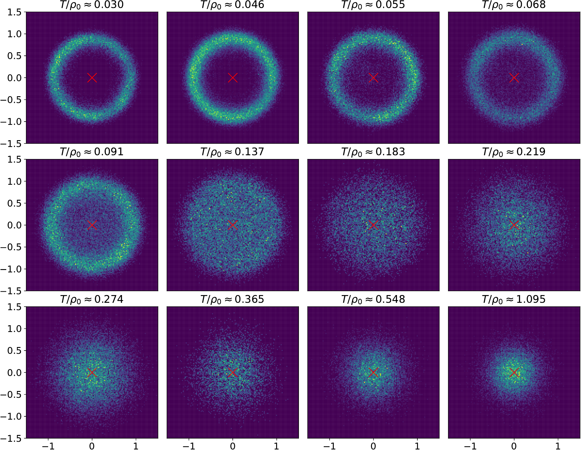
Figure 2: Distributions of $\frac{1}{\rho_{0}N_{\mathrm{s}}N_{\mathrm{t}}}\sum_{t,x}\Delta(t,x)$ in the complex plane for 2 flavors, $N_{s}=63$, $a\approx 0.46$ and $\mu=0$ at various temperatures. The red crosses mark the origin and are included for visual clarity.

We shall see that for $8$ flavors the correlation function $C(x)$ in (22) has the form (30) predicted by the effective low-energy Lagrangian and can be hardly distinguished from the large-$N_{\mathrm{f}}$ result (23). For example, at low temperature its discrete Fourier transform $\mathcal{F}[C](k)$ is peaked at the dominant wave number

$$k_{\mathrm{max}}=\frac{1}{2}\underset{k}{\mathrm{argmax}}\,|\mathcal{F}[C](k)|\;,$$ (33)

which for large $N_{\mathrm{f}}$ is given by the chemical potential,

$$k_{\mathrm{max}}\stackrel{{\scriptstyle N_{\mathrm{f}}\to\infty}}{{\longrightarrow}}\mu\;,$$ (34)

while for $N_{\mathrm{f}}=2$ we find $k_{\mathrm{max}}<\mu$. Notice that we have included a factor of $1/2$ in Eq. (33), in line with the introduction of $k$ in Eq. (19) as half the wave number. We will use this convention for $k$ and $k_{\mathrm{max}}$ in the remainder of this work.

The spatial correlation function $C(x)$ also encodes the distinction between the massive symmetric and BKT phases in its decay properties,

$$|C(x)|\stackrel{{\scriptstyle x\to\infty}}{{\longrightarrow}}\begin{cases}e^{-x/\xi_{\beta}}&\text{massive symmetric}\;,\\ x^{-\frac{1}{N_{\mathrm{f}}}}&\text{BKT}\;,\\ \mathrm{const.}&\text{symmetry-broken}\;.\end{cases}$$ (35)

For a comparison we included the asymptotic behavior in a symmetry-broken phase. The temperature-dependent correlation length $\xi_{\beta}$ was defined in Eq. (32).

III.2 Lattice setup

We discretize two-dimensional Euclidean spacetime to a finite lattice with $N_{s}$ and $N_{t}$ lattice sites in the spatial and temporal directions respectively, such that $L=N_{s}a$ is the spatial extent, $T=1/N_{t}a$ is the temperature and $a$ denotes the lattice constant.

In our simulations we employ chiral SLAC fermions Drell et al. (1976a, b), which discretize the dispersion relation in momentum space, leading to a non-local kinetic term in position space. They have proven advantageous over other fermion discretizations for low-dimensional fermionic theories, see e.g. Lenz et al. (2020a). The use of SLAC fermions restricts $N_{s}$ to be odd and $N_{t}$ to be even. For further details we refer to sections 2.1 and 4.1 of Bergner et al. (2008). Note that our lattice setup is the same as in Lenz et al. (2020a), with the only difference that besides a scalar field $\sigma$ we now have an additional pseudo-scalar field $\pi$ and both fields enter the complex condensate field $\Delta$ via Eq. (7).

For an easy comparison with the analytic results we express physical quantities in units of the expectation value $\left\langle\rho\right\rangle$ at $T=\mu=0$, denoted by $\rho_{0}$. This is analogous to the scale $\sigma_{0}$ in our previous studies Lenz et al. (2020a, b). One should stress that this neither assumes any form of symmetry breaking nor is in conflict with any no-go theorem because a non-vanishing expectation value of $\rho$ does not break any symmetry. Fig. 2 shows histograms of $\sum_{\boldmathe{x}}\Delta(\boldmathe{x})$ in the complex plane for $\mu=0$ and $12$ different temperatures. For these histograms we used ensembles with $\mathcal{O}(10^{4})$ configurations each. We clearly observe that the distribution of $\Delta$ is angle independent or U_A(1) invariant. At low temperature it is ring shaped with its maximum at $\rho>0$, while at high temperature it turns into a Gaussian-like distribution and the maximum moves to $\rho=0$.

In the actual simulations, however, the quantity $\rho_{0}$ is surprisingly hard to determine. App. A sheds some light on the details of this procedure. In summary, we used

$$\left\langle\rho\right\rangle\approx\frac{1}{N_{\mathrm{s}}N_{\mathrm{MC}}}\sum_{\tau,x}\Big{|}\frac{1}{N_{\mathrm{t}}}\sum_{t}\Delta^{(\tau)}(t,x)\Big{|}\;,$$ (36)

with $\tau=1,\dots,N_{\mathrm{MC}}$ enumerating the Monte Carlo (MC) configurations. This yields a good signal at low temperatures where $\langle\rho\rangle$ is required.

For most of our simulations, we used one of three different spatial extents $N_{\mathrm{s}}=63,127,255$ and lattice constants $a\rho_{0}\approx 0.46$, $0.19$, $0.08$ in order to study both the continuum limit and the infinite-volume limit. We vary the temperature by changing the number of lattice points in the temporal direction, $N_{\mathrm{t}}$, at fixed $a$ and we vary $a$ by changing the coupling $1/g^{2}$ in Eq. (8). For these lattices we map out phase diagrams in the $(T,\mu)$ plane. More details as well as a table summarizing all parameter settings are given in App. D.

Experience with interacting fermion models teaches us Lenz et al. (2020a) that systems exhibiting (quasi-)long-range inhomogeneous structures can have rather long thermalization times when running simulations with randomly generated initial configurations, e.g., using a Gaussian distribution. As a way to counteract this problem, we employ a different approach for the majority of results presented in this work and perform a systematic ”freezing out” in the following way: Starting at high temperatures with $N_{\mathrm{t}}\ll N_{\mathrm{s}}$, where thermalization times are not an issue, we generate at least $1000$ configurations to ensure proper thermalization. We then map the last of these configurations to a lower-temperature lattice with $N_{\mathrm{t}}^{\prime}>N_{\mathrm{t}}$ by simply repeating the data in the temporal direction and use it as a seed configuration on the larger lattice. This reduces the thermalization period (where no measurements are performed) if the temperature step is small. In our simulations we systematically approach lower and lower temperatures using this ”freeze-out” procedure. This way we experienced significantly less ”getting stuck” in some far from typical configurations, although it could still not be completely prevented from happening.

A cross-check with thermalized results using standard Gaussian-distributed initial configurations yields equivalent results, with the ”freezing” method having noticeably better thermalization properties and thus overall smoother results. As an additional cross-check we also performed the inverse procedure, i.e., a ”heating”, for a handful of parameters in order to exclude any hysteresis effects caused by the ”freezing” method.

As can be seen from Fig. 3, where we show the Fourier transform of $C_{\sigma\sigma}(x)$ (to be defined in Eq. (37)) computed via each of the three methods, the ”frozen” and ”heated” results agree very well, indicating that hysteresis effects are negligible. The fact that the ”independent” results, i.e. the ones obtained by using Gaussian-distributed initial configurations, show some deviation is likely to be attributed to their lower statistics and worse thermalization properties.

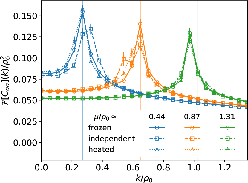
Figure 3: The Fourier transform of $C_{\sigma\sigma}(x)$ as a function of $k$ for the three different methods mentioned in the main text on a $48\times 127$ lattice for $a\rho_{0}\approx 0.46$ and different $\mu$. The temperature is the second lowest considered, i.e. we compare several ”freezing” steps with a single ”heating” step. The vertical lines indicate the maxima of the ”frozen” results at the lowest temperature.

The vertical lines in Fig. 3 show the peak positions, which were estimated with the ”freezing” method, for the lowest temperature considered. We see that for the highest density ($\mu/\rho_{0}\approx 1.31$ in the figure) the peak positions of the two lowest temperatures differ. This dependence on temperature is not seen in the large-$N_{\mathrm{f}}$ limit and is caused by bosonic fluctuations.

For small $\mu$ on our smallest lattice, where homogeneous configurations dominate, we furthermore compared with a ”cold start”, which amounts to starting the simulation from $\Delta^{(0)}(t,x)=1+\mathrm{i}$. Again we found matching results except for the lowest temperatures where the cold start is expected to suffer from severe autocorrelation problems. A detailed analysis of autocorrelation effects can be found in App. B.

III.3 Lattice estimators

We have argued that spatial correlation functions are useful tools to probe for inhomogeneous phases since they avoid the destructive interference one would encounter when directly calculating chiral condensates on the lattice. We consider the two spatial correlators

$$\begin{aligned} C_{\sigma\sigma}(x)&=\frac{1}{N_{t}N_{s}}\sum_{t,y}\langle\sigma(t,y+x)\sigma(t,y)\rangle\;,\\ C_{\sigma\pi}(x)&=\frac{1}{N_{t}N_{s}}\sum_{t,y}\langle\sigma(t,y+x)\pi(t,y)\rangle\;,\end{aligned}$$ (37)

where the sums extend over all lattice sites and $\langle\,\cdot\,\rangle$ denotes the Monte Carlo average. If these correlators show an oscillating behavior, one can infer the existence of inhomogeneities. The unbroken U_A(1) symmetry (5) implies that for any temperature and chemical potential

$$C_{\sigma\sigma}(x)=C_{\pi\pi}(x)\quad\text{and}\quad C_{\sigma\pi}(x)=-C_{\pi\sigma}(x)\;.$$ (38)

Also note that the fermion determinant is invariant when $\sigma$ and $\mu$ both change their signs, such that

$$\langle\sigma(\boldmathe{x})\pi(\boldmathe{y})\rangle_{\mu}=-\langle\sigma(\boldmathe{x})\pi(\boldmathe{y})\rangle_{-\mu}\;,$$ (39)

from which we conclude that

$$C_{\sigma\pi}(x)=C_{\pi\sigma}(x)=0\quad\text{for}\quad\mu=0\;.$$ (40)

We see that additional correlators that arise from interchanging $\sigma\leftrightarrow\pi$ in Eq. (37) are not independent and we refrain from using them in subsequent equations to save some space. In the measurements, however, we do not implement the symmetries (38) and instead use all four correlators $C_{\sigma\sigma}$, $C_{\sigma\pi}$, $C_{\pi\sigma}$ and $C_{\pi\pi}$ in order to reduce statistical correlations. From Eq. (22) one obtains

$$C(x)=2(C_{\sigma\sigma}(x)+\mathrm{i}\,C_{\sigma\pi}(x))$$ (41)

and the property (40) means that $C$ is real for vanishing $\mu$.

In Lenz et al. (2020a) we introduced the minimal value

$$C_{\min}=\min_{x}C_{\sigma\sigma}(x)\begin{cases}>0&\text{homogeneous}\\ \approx 0&\text{symmetric}\\ <0&\text{inhomogeneous}\end{cases}$$ (42)

to map out the entire phase diagram of the (discrete) GN model. This parameter is negative if there is (quasi-) long-range order with oscillating $C_{\sigma\sigma}(x)$ and is also useful for discussing the physics of the chiral GN model. For the chiral model the choice of $C_{\sigma\sigma}$ might seem arbitrary but because of (38) any quadratic correlator of a linear combination of $\sigma$ and $\pi$ would serve the same purpose.

It is important to note that taking the minimum is a global operation that disqualifies this quantity as a local observable. Furthermore, this minimum might (and actually commonly will) be taken for small spatial separations $x$. In such cases, $C_{\min}$ does not probe the long-range behavior of the system.

We estimate the dominant wave number $k_{\mathrm{max}}$ as given by Eq. (33), but calculated from $C_{\sigma\sigma}$ instead of $C$. Sometimes we quote results in terms of the integer-valued dominant winding number $\nu_{\mathrm{max}}$, related to $k_{\mathrm{max}}$ via

$$\nu_{\mathrm{max}}=\frac{L}{\pi}k_{\mathrm{max}}\;.$$ (43)

From analytical studies Andersen (2005); Witten (1978) it is expected that the U_A(1)-invariant fermionic four-point function of the GN model,

$$C_{\mathrm{4F}}(\boldmathe{x};\boldmathe{y})=\left\langle\bar{\psi}(1+\gamma_{*})\psi(\boldmathe{x})\bar{\psi}(1-\gamma_{*})\psi(\boldmathe{y})\right\rangle\;,$$ (44)

at zero temperature and zero fermion density should have a power-law behavior in the limit of large separations,

$$C_{\mathrm{4F}}(\boldmathe{x};\boldmathe{y})\sim c\,|\boldmathe{x}-\boldmathe{y}|^{-\frac{1}{N_{\mathrm{f}}}}\;,$$ (45)

where $c$ is some constant. Similarly to the spatial correlation functions (37) for the condensate fields we introduce the spatial correlation function for the $N_{\mathrm{f}}$ fermionic lattice fields,

$$C_{\mathrm{4F}}(x)=\frac{1}{N_{t}N_{s}}\sum_{t,y}C_{\mathrm{4F}}(t,y+x;t,y)\;.$$ (46)

The asymptotic form (45) would imply a power-law decay

$$C_{\mathrm{4F}}(x)\sim c\,x^{-\frac{1}{N_{\mathrm{f}}}}\quad\text{for}\quad x\gg 1\;.$$ (47)

Dyson-Schwinger equations (see App. 64) relate $C_{\mathrm{4F}}(x)$ to the spatial correlation functions of the condensate fields,

$$C_{\mathrm{4F}}(x)=-2\left(\frac{N_{\mathrm{f}}}{g^{2}}\right)^{2}\left(C_{\sigma\sigma}(x)+\mathrm{i}\,C_{\sigma\pi}(x)\right)\;,$$ (48)

since the contact term in Eq. (64) does not contribute for large $x$. Since $C_{\sigma\sigma}$ and $C_{\sigma\pi}$ are easily accessible in lattice simulations we shall use this relation to study the infrared properties of $C_{\mathrm{4F}}$. For $\mu=0$ the latter is real, see (40).

From the effective low-energy approximation outlined in Sec. II.4 we expect that the phase of the complex condensate field, $\theta=\arg(\Delta)$, holds important information about the existence of inhomogeneous structures. We thus studied the space dependence of its expectation value, defined in the following way:

$$\left\langle\theta(x)\right\rangle=\arg\left(\left\langle\bar{\Delta}(x)\right\rangle\right)\;,$$ (49)

where the bar indicates time averaging, i.e.,

$$\bar{\Delta}(x)=\frac{1}{N_{t}}\sum_{t}\Delta(t,x)\,.$$ (50)

We chose this (unusual) order of time- and MC averaging to suppress statistical uncertainties. Although the two averages in (49) do not commute the given prescription is justified since the configurations are essentially constant in time direction, see Fig. 4 for an example configuration of the $\sigma$ field.

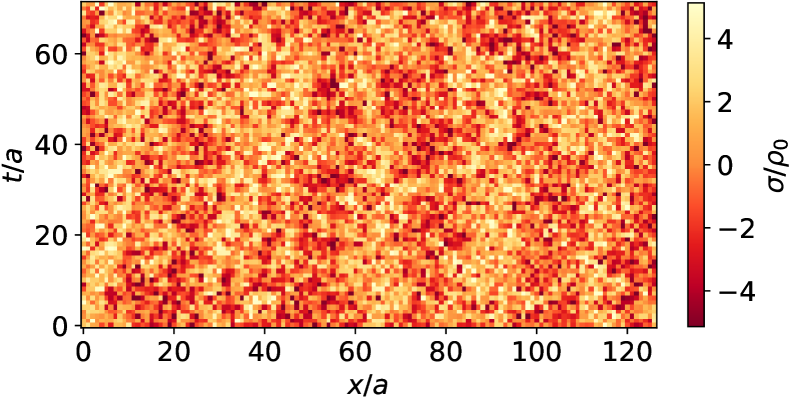
Figure 4: Typical configuration of $\sigma(\boldmathe{x})$ on a $72\times 127$ lattice for $\mu/\rho_{0}\approx 0.44$ and $a\rho_{0}\approx 0.46$.

IV Numerical Results

In previous studies of the discrete GN model Lenz et al. (2020a, b), $2$, $8$ and $16$ flavors have been investigated with the focus on $N_{\mathrm{f}}=8$ in order to compare different types of chiral fermions and their suitability to investigate inhomogeneous phases. But $N_{\mathrm{f}}=8$ is still close to $N_{\mathrm{f}}=\infty$ in the sense that on an intermediate scale quantum fluctuations away from the chiral spiral are suppressed. To be more precise, if the BKT scenario were correct, then, for instance, in order to obtain a decay to half the amplitude a crude estimate using $C(x)\sim|x|^{-1/8}$ yields

$$\frac{C(x^{\prime})}{C(x)}=\frac{1}{2}\quad\Rightarrow\quad|x^{\prime}|=256\,|x|$$ (51)

at the very least. Thus, in order to make any meaningful statements about such an amplitude decay we would require around $\mathcal{O}(10^{3})$ lattice points at sufficiently small temperature (large temporal extent). This does not take into account severe autocorrelation problems, finite-size effects and contributions from excited states that might all spoil the signal. This crude estimate motivated us to study the long-range behavior for $N_{\mathrm{f}}=2$ in Lenz et al. (2020a), for which the same estimate yields feasible 40 lattice points.

(a) Phase diagram via $C_{\min}$ from Eq. (42).

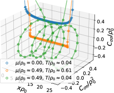
(b) Correlators $C_{\sigma\sigma}(x)$ and $C_{\sigma\pi}(x)$ from Eq. (37) for various representative parameters.

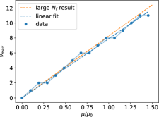
(c) Dominant winding number $\nu_{\mathrm{max}}$ from Eq. (43) and Eq. (33) for $T/\rho_{0}\approx 0.030$. The linear fit has a slope of $7.91\pm 0.10$.

Figure 5: Collection of results for $N_{\mathrm{f}}=8$, $N_{\mathrm{s}}=63$, $a\rho_{0}\approx 0.41$.

IV.1 Overview for $N_{\mathrm{f}}=8$

Although our focus is on $2$ flavors we performed one parameter scan in $(T,\mu)$ for $N_{\mathrm{f}}=8,\ N_{\mathrm{s}}=63$ and $a\rho_{0}\approx 0.41$ in order to compare with results for the discrete GN model. Some of our results are depicted in Fig. 5. Fig. 5(a) shows the phase diagram extracted from $C_{\min}$ (see Eq. (42)), which is to be compared with Fig. 1 for infinite flavor number and is also the equivalent of Fig. 7 in Lenz et al. (2020a). We see that the phase diagram agrees well with the large-$N_{\mathrm{f}}$ prediction for small chemical potential ($\mu<0.5\rho_{0}$) and at least shows the predicted structure at larger $\mu$.

At vanishing chemical potential $C_{\min}$ is positive for small temperatures, indicating predominantly homogeneous configurations with non-vanishing amplitudes. They relate to the homogeneously symmetry-broken phase at large $N_{\mathrm{f}}$. In Fig. 5(b) we see that in this regime $C_{\sigma\sigma}(x)$ is a positive and monotonically decaying function (blue curve) and $C_{\sigma\pi}(x)\approx 0$ in agreement with (40). Raising the temperature we find a small temperature regime around $T\sim 0.3\rho_{0}$ where we observe a sudden drop of the amplitude such that the $\mu=0$ data mimic a second-order phase transition. In the high-temperature regime the non-zero correlator $C_{\sigma\sigma}$ falls off even more rapidly. This (would-be) transition temperature at $\mu=0$ is approximately equal to the one found in the discrete GN model in Lenz et al. (2020a). This was to be expected since in the large-$N_{\mathrm{f}}$ limit the GN and cGN models at vanishing chemical potential have the same critical temperature. It is also not surprising that for $N_{\mathrm{f}}=8$ the transition temperature is significantly lower than in the large-$N_{\mathrm{f}}$ limit (cf. Eq. (18)), where quantum fluctuations are suppressed. The symmetric high-temperature regime at $\mu=0$ extends to non-vanishing chemical potential (orange curve in Fig. 5(b)).

At low temperature and non-vanishing fermion density we can clearly confirm that the dominant contributions to the path integral come from chiral–spiral-like configurations. An example of this is shown in Fig. 5(b) (green curve). Such configurations are the cause of the large region of negative values in Fig. 5(a). The transition line to the region where oscillations are no longer dominant is roughly a line of constant temperature for small chemical potential ($\mu<0.5\rho_{0}$), as expected from the large-$N_{\mathrm{f}}$ solution. For large chemical potential it tilts upwards unexpectedly, thereby enlarging the regime where inhomogeneities are found. This effect was also observed in Lenz et al. (2020a) for $N_{\mathrm{f}}=2$ in the discrete GN model and is related to short- and intermediate-range phenomena that will be discussed later. Nevertheless, the fact that we encounter it already for $N_{\mathrm{f}}=8$ strengthens the point that quantum fluctuations are much stronger in the chiral model compared to the discrete one.

For $N_{\mathrm{f}}=8$ the winding numbers (43) of the inhomogeneous configurations match the large-$N_{\mathrm{f}}$ expectation very well if one accounts for the discretization of the wave number due to the finite box size, as can be seen in Fig. 5(c) (note that $\nu_{\mathrm{max}}$ is integer valued by definition). As in Lenz et al. (2020b) there is a tendency for the lattice data to lie slightly below the $N_{\mathrm{f}}=\infty$ expectation. The linear fit through the origin yields a slope of roughly $7.91$, which is lower than the large-$N_{\mathrm{f}}$ value $L/\pi\approx 8.27$, but well within the expected accuracy of the large-$N_{\mathrm{f}}$ expansion $\mathcal{O}(1/N_{\mathrm{f}})\sim 10\%$.

We remark that autocorrelations appear to be under control. However, due to limited statistics we cannot rule out the existence of another, larger, autocorrelation scale at low temperatures, see App. B for details.

IV.2 Deviations of $N_{\mathrm{f}}\!=\!2$ from the large-$N_{\mathrm{f}}$ limit

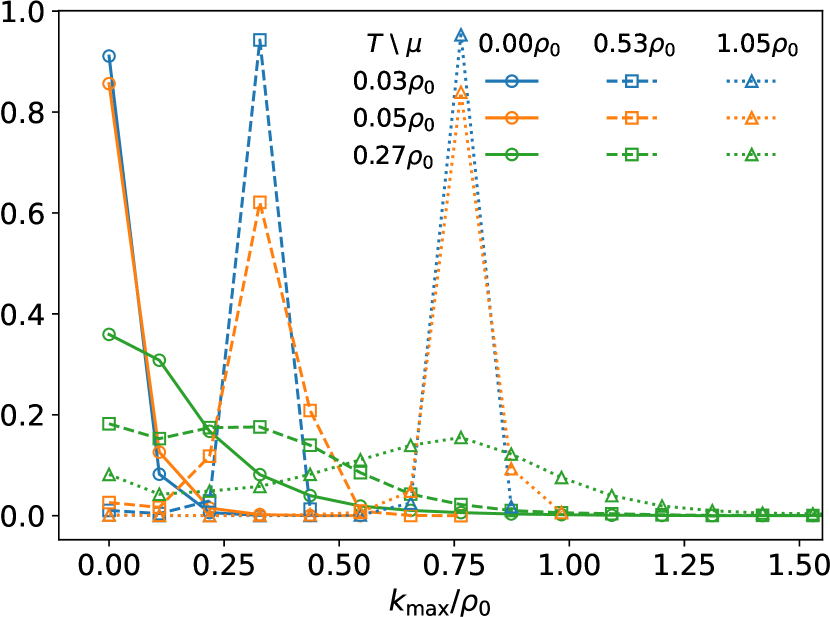
Figure 6: Histograms of $k_{\mathrm{max}}$ for $N_{\mathrm{f}}=2$, $N_{\mathrm{s}}=63$, $a\rho_{0}\approx 0.46$ and various values of temperature and chemical potential.

(a)

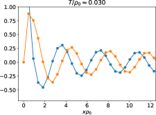
(b)

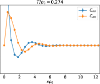
(c)

Figure 7: Correlators $C_{\sigma\sigma}$ and $C_{\sigma\pi}$ (from Eq. (37)) for $N_{\mathrm{f}}=2$, $N_{\mathrm{s}}=63$, $\mu/\rho_{0}\approx 1.14$ and $a\rho_{0}\approx 0.46$. (a): 3D plot of the correlators at $T/\rho_{0}\approx 0.030$ showing the chiral spiral. (b): The same data as in (a) but in 2D. (c) 2D plot of the correlators at higher temperature.

After discussing the results for $N_{\mathrm{f}}=8$, which in many ways confirm the large-$N_{\mathrm{f}}$ expectations, we now study the $2$-flavor cGN model for which we expect sizable deviations from the large-$N_{\mathrm{f}}$ solution.

To monitor the fluctuations in the system at finite temperature and density, we measure the dominant wave number (33) of the equilibrium ensemble. It characterizes important configurations for the given set of control parameters and tells us which chiral spiral is favored in the rough landscape defined by the effective action with its many local minima. This analysis presupposes that chiral spirals are the dominant configurations even for $N_{\mathrm{f}}=2$ or that the non-dominant winding numbers are suppressed. We shall see that this is a valid assumption at small temperatures.

Fig. 6 shows such histograms for $3$ values of $T$ and $3$ values of $\mu$. As expected, the data show three distinct peaks, one for each value of $\mu$. At the lowest temperature and $\mu\neq 0$ the peaks are pronounced with over $80\%$ of the configurations sharing the same dominant wave number. Increasing the temperature then broadens the peaks. Concerning the question of spontaneous symmetry breaking, one should stress three features:

1. While the peaks flatten significantly for rising temperature, they do not vanish completely. At temperatures as high as $\sim 0.5\rho_{0}$ we could still make out small bumps (not shown in Fig. 6). Thus, even at these high temperatures the system knows about the inhomogeneity arising from its finite density.

2. There is no qualitative (or even sudden) change in these distributions that could characterize a second-order phase transition. Instead the flattening of the peaks is a rather smooth process.

3. Even at low temperatures (e.g. $T\approx 0.05\rho_{0}$), well inside the would-be symmetry-broken regime, the contributions from concurrent frequencies are significant (around $10-20\%$ in the example). The interference of these contributions is the mechanism which, crucially, prevents a breaking of symmetry.

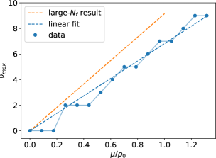
Figure 8: $\nu_{\mathrm{max}}$ as a function of $\mu$ for $N_{\mathrm{f}}$=2, $N_{\mathrm{s}}=63$, $a\rho_{0}\approx 0.46$ and $T/\rho_{0}\approx 0.030$. The linear fit has a slope of $6.82\pm 0.17$.

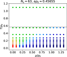
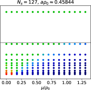
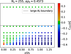
Figure 9: Infinite-volume extrapolation: phase diagrams for fixed lattice spacing and $N_{s}=63,127$ and $255$.

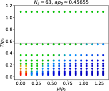
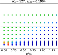
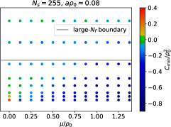
Figure 10: Continuum extrapolation: phase diagrams for decreasing lattice constant. The color coding is different from Fig. 9.

The features 1 and 2 discussed above are clearly visible in the spatial correlators depicted in Fig. 7. At low $T$ and non-vanishing $\mu$ we clearly observe remnants of a chiral spiral, see Fig. 7(a). From Fig. 7(b) we see that both correlators are oscillating with a phase shift of $\pi/2$. This is the parameter region where there are sharp peaks in Fig. 6. At higher temperature the peaks flatten and the correlators show damped oscillations as shown in Fig. 7(c). Notice, however, that even in this regime we still find $C_{\min}<0$, i.e., this is classified as a region of spatial inhomogeneities according to our definition. Here we observe a clear deviation from the large-$N_{\mathrm{f}}$ solution. Since the oscillations in Fig. 7(c) are only seen on short scales we must be cautious when interpreting a negative $C_{\min}$ as a signal for inhomogeneities. As already stressed before, a negative $C_{\min}$ ensures that there are oscillations on some length scale but this scale can be – and certainly is for large parts of the blue region of the phase diagram – a short or intermediate one. Finally, at even higher temperatures one again finds correlation functions with $C_{\min}\approx 0$, indicating a symmetric region.

Similarly to $N_{\mathrm{f}}=8$ we determined the dependence of the dominant winding number in Eq. (43) on the chemical potential and we present the results in Fig. 8. As expected, the (dominant) winding numbers for $N_{\mathrm{f}}=2$ deviate considerably from those in the large-$N_{\mathrm{f}}$ limit and those for $N_{\mathrm{f}}=8$, cf. Fig. 5(c). One might conjecture that the winding numbers decrease with decreasing $N_{\mathrm{f}}$.

IV.3 Phase diagram for $N_{\mathrm{f}}\!=\!2$

One could expect a qualitatively different ”phase diagram” for the cGN model with $2$ flavors as compared to the large-$N_{\mathrm{f}}$ diagram depicted in Fig. 1. In order to test this expectation we calculated $C_{\min}$ defined in Eq. (42) on a grid in the space of control parameters $\mu$ and $T$ on lattices with $N_{s}=63$, $127$ and $255$ lattice points in the spatial direction. We studied both an infinite-volume extrapolation at (approximately) fixed lattice constant $a\rho_{0}\approx 0.46$ and a continuum extrapolation at (approximately) fixed physical volume.

The diagrams for systems with constant lattice spacing in Fig. 9 show that the infinite-volume limit significantly shrinks the red ($C_{\min}>0$, i.e. predominant homogeneous contributions) region without affecting the blue and green region of predominant inhomogeneous resp. symmetric configurations. There are three rather different phenomena at work here:

1. The simplest one is just geometrical: When we enlarge the spatial volume, we can fit larger wavelengths into the finite box. For small $\mu$ the pitch of the chiral spiral would exceed the box size, which means that the chiral spiral does not fit into the box. Such a suppression of chiral spirals with large pitches disappears for larger volumes. Hence, the region of predominant homogeneous configurations must shrink in the direction of non-vanishing $\mu$.

2. Finding a shrinking of the $C_{\min}>0$ region in the temperature direction is clear evidence against spontaneous symmetry breaking. In fact, the (qualitative) behavior of the apparent transition temperature and the condensate is well understood by a comparison of the analytically known correlation length Eq. (32) with the box size. We can thereby clearly identify the remnant condensates that were measured as finite-size effects.

3. The transition from the blue ($C_{\min}<0$, i.e. predominant inhomogeneities) to the green ($C_{\min}\approx 0$, i.e. predominantly symmetric) regime can be easily understood as the following short-range effect: At finite temperature there are two length scales in the system (besides the finite box size), i.e. the temperature-induced finite correlation length $\xi_{\beta}$ from Eq. (32) and the predominant wavelength inversely proportional to $\mu$ (up to discretization due to the finite box size). Obviously, for $C_{\min}$ to be negative, the amplitude, which decays due to $\xi_{\beta}$, must not have dropped to (almost) vanishing values at separations where the first minimum of the oscillations occurs. Since the latter is given by $\mu$ (up to a constant factor), the transition line from blue to green signals that the temperature scale takes over as the shortest relevant scale from the chemical potential. This is not really a qualitative change. As this is independent of the much larger box size, it is not affected by the infinite-volume limit.

An interesting, but unfortunately hard to quantify observation is the following. While on smaller lattices (e.g. $N_{\mathrm{s}}=63$) the data tend to fluctuate around only one background configuration, like a chiral spiral with a fixed winding number, larger lattices admit changing the winding number more often as opposed to less often. An example is depicted in Fig. 11, which shows a time series of the modulus $\rho^{(\tau)}$ of the spacetime average of $\bar{\Delta}^{(\tau)}$ defined in Eq. (58) of App. A. Even for vanishing chemical potential and low temperature, the regime in the phase diagram where we set the scale and where the dominant configurations are homogeneous, we still find several occasions on which there are dominant inhomogeneous contributions.

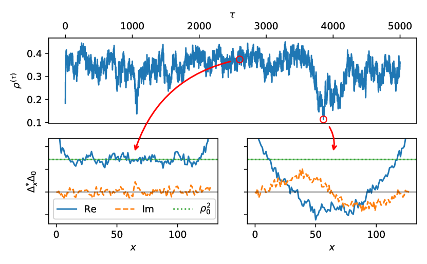
Figure 11: Monte Carlo time series of $\rho^{(\tau)}$ defined in (58) (top) with the $\Delta_{x}^{*}\Delta_{0}$ correlator at $\tau=2604$ (bottom, left) and $\tau=3856$ (bottom, right) for $N_{\mathrm{t}}=72$, $N_{\mathrm{s}}=255$, $g^{-2}=1.0540$ and $\mu=0$.

For most of the MC time $\rho^{(\tau)}$ fluctuates about a constant value. During this time the real part $C_{\sigma\sigma}$ of $C$ defined in (22) is almost constant and the imaginary part $C_{\sigma\pi}$ is small (recall that $\langle C_{\sigma\pi}\rangle=0$). But at several MC times, e.g. $\tau\approx 1100$ or $3860$, the field $\rho^{(\tau)}$ drops and the real and imaginary parts of $C(x)$ show the profiles typical for a chiral spiral. While the lower left plot in Fig. 11 is representative for most of the configurations, the sudden drops in the time series are strongly correlated with the appearance of inhomogeneous configurations as seen in the lower right panel. That this is only seen on large lattices is counterintuitive at first since autocorrelation times usually increase with the system size and it is also the opposite of what was observed for the $\mathbb{Z}_{2}$ GN model during the work on Lenz et al. (2020a, b). However, the fact that considerable phase fluctuations on large scales are allowed is the analytically predicted mechanism for avoiding spontaneous symmetry breaking, see Sec. II. From that perspective, it supports the analytical claims. Obviously, Fig. 11 showcases a large autocorrelation time $\tau$, which, however, is under control due to good statistics of the order of $\gtrsim 20\tau$.

The phase diagrams for systems with approximately constant physical volume and successively smaller lattice spacing are shown in Fig. 10. As can be seen, we find inhomogeneities for all our lattice spacings and the results are consistent with their existence in the continuum limit. Unfortunately, setting the scale in a partially conformal system is a very subtle issue as the dominant fluctuations have no scale at all (at zero temperature). Since the details of this scale setting procedure are highly non-trivial (see App. A), we must leave a more detailed analysis to a future publication.

As is discussed in detail in App. B, our simulations suffer from large autocorrelations. For a large region in parameter space on all geometries these autocorrelations are under control due to sufficient statistics. However, close to the critical line at $T=0$ autocorrelation times diverge and the shown data should only be regarded as qualitative in the sense that they surely capture the important phenomena found in large but finite regions of space but might be off quantitatively due to autocorrelation-related suppression of subdominant local minima. However, the discussion of App. B makes it clear that these will not affect our conclusions.

We conclude that we observe inhomogeneous structures in the cGN model with only $2$ flavors – similarly as in the large-$N_{\mathrm{f}}$ model. The notable difference is that – in accordance with pertinent no-go theorems – these are incoherent on sufficiently large scales thereby hindering spontaneous symmetry breaking. A comparable study of the $\mathbb{Z}_{2}$ GN model with $8$ flavors in Lenz et al. (2020a) led to a similar conclusion: inhomogeneous structures persist in the infinite volume limit. We cannot say for certain whether this remarkable feature survives the continuum limit of the cGN lattice models.

IV.4 Decay properties of $C_{\mathrm{4F}}$

We analyzed the decay properties of $C_{\mathrm{4F}}(x)$ as given by Eq. (48) on a $72\times 63$ lattice with $a\rho_{0}\approx 0.46$, i.e. at a temperature $T\approx 0.03\rho_{0}$. In order to study its infrared behavior we computed the connected correlation function. Motivated by the asymptotic forms (31) predicted by the low-energy effective action we fit the data points via a (symmetrized) algebraic function

$$C_{\mathrm{4F}}(x)=\frac{\alpha}{x^{\beta}}+\frac{\alpha}{(L-x)^{\beta}}\;,$$ (52)

as well as a double-cosh ansatz,

$$C_{\mathrm{4F}}(x)=\sum_{i=1}^{2}\gamma_{i}\cosh\left[m_{i}\left(x-\frac{L}{2}\right)\right]\;,$$ (53)

and show the results in Fig. 12.

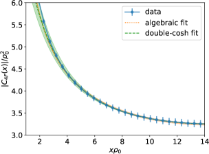
Figure 12: Modulus of the connected four-point function $C_{\mathrm{4F}}$ (from Eq. (48)) with algebraic and exponential fits whose fit parameters are given in (54) and (55).

The fit parameters for a power-law decay are

$$\frac{\alpha}{\rho_{0}^{2}}=6.52\pm 0.02\;,\quad\beta=0.521\pm 0.001$$ (54)

and for an exponential decay we find

$$\begin{aligned} \frac{\gamma_{1}}{\rho_{0}^{2}}=3.2515\pm 4\cdot 10^{-4}\;,\quad&\frac{m_{1}}{\rho_{0}}=(5.76\pm 0.03)\cdot 10^{-2}\;,\\ \frac{\gamma_{2}}{\rho_{0}^{2}}=(4.4\pm 0.3)\cdot 10^{-3}\;,\quad&\frac{m_{2}}{\rho_{0}}=0.531\pm 0.006\;.\end{aligned}$$ (55)

These results confirm similar findings obtained for the $\mathbb{Z}_{2}$ GN model, namely that it is very difficult to distinguish between power-law and exponential decays on the lattices with $N_{s}=63$, which was also to be expected following the previous discussion and Bramwell and Holdsworth (1994). However, from the perspective of our analytical discussion, where we predicted a massive phase for any $T>0$ with the mass vanishing in the limit $T\to 0$, there is a very well-motivated explanation. Eq. (32) predicts

$$m_{1}=1/\xi_{\beta}\approx 2\cdot 10^{-2}\rho_{0}\;,$$ (56)

which is reasonably close to the fitted value (remember that we expanded in $\mathcal{O}(1/N_{\mathrm{f}})\sim 50\%$ for $N_{\mathrm{f}}=2$) and explains its seemingly unnaturally small magnitude.

On the other hand, we find that the value $\beta\approx 0.52$ is only marginally larger than the theoretical zero-temperature prediction of $\beta=0.5$ for two flavors in Eq. (35). This result – although not precisely a proof – is in astonishing agreement with the analytical prediction coming from an expansion around $N_{\mathrm{f}}=\infty\gg 2$ and furthermore beautifully reveals how the massive phase more and more approximates the conformal behavior at zero temperature by the unexpectedly large mass ratio $m_{2}/m_{1}\approx 10$.

IV.5 The phase field $\theta$

In this section we analyze $\left\langle\theta(x)\right\rangle$. This discussion should be regarded as complementary to the previous analysis of the correlators in the sense that we now use a quantity directly related to the fields. It will further substantiate our previous findings.

We show the $x$ dependence of the average $\langle\theta(x)\rangle$, as defined in Eq. (49), on a $72\times 63$ lattice for $a\rho_{0}\approx 0.46$ and for three values of the chemical potential in Fig. 13. For vanishing $\mu$ the argument of the averaged complex condensate field $\Delta$ is constant, which means that the latter does not wind. For the intermediate value $\mu\approx 0.88\rho_{0}$ the average angle is an almost linear function of $x$ and the complex condensate winds $6$ times when one moves along the spatial direction. When one further increases the chemical potential to $\mu\approx 1.31\rho_{0}$, the slope of the (almost) linear mapping $x\mapsto\langle\theta(x)\rangle$ increases and the condensate winds $9$ times.

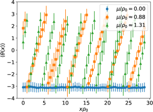
Figure 13: Angle of the averaged scalar field, $\langle\theta\rangle=\arg(\langle\bar{\Delta}\rangle)$, calculated from time-averaged fields $\bar{\sigma}$ and $\bar{\pi}$, as a function of the spatial coordinate for different $\mu$ at $N_{t}=72$.

We see that the winding number of the chiral spiral around the spatial direction increases with increasing $\mu$. In fact, the winding number extracted from the averaged field $\langle\theta(x)\rangle$ perfectly agrees with the dominant winding number defined in Eq. (43) and depicted in Fig. 8. To summarize: at low temperature $\langle\theta(x)\rangle$ calculated from (49) is almost a linear function of $x$ with a slope proportional to $\mu$. In agreement with the analysis based on the dominant wave number we detect a chiral spiral with a winding number proportional to $\mu$.

V Conclusions

In the present work we studied the $(1+1)$-dimensional chiral Gross-Neveu model with chiral SLAC fermions and exact axial U_A(1) symmetry on the lattice. Our two main results are summarized in the following.

First, we have strong and multiple evidence that the analytical prediction from an expansion in $1/N_{\mathrm{f}}$ well describes the qualitative features of the cGN model with $2$ flavors. As expected we see no spontaneous symmetry breaking with long-range order in the strict sense, and our results suggest that at $T=0$ there is a BKT phase with quasi-long-range order. For example, the low-temperature regime, where we have signals of (in)homogeneous ordering over the whole lattice, is well explained by the analytically predicted correlation length exceeding the finite box size and it shrinks consistently in the thermodynamic limit. Additionally, the decay properties of pertinent correlation functions are well fitted by the analytically predicted ansätze with reasonable parameter values.

The latter suggests that for $T=0$ fluctuations of the phase field $\theta$ on all scales exist and are responsible for the restoration of the axial symmetry. We demonstrated that $\theta$ is uniformly distributed on unit circles in complex field space and that large system sizes allow for long-range phase fluctuations strong enough to change the winding number. This behavior is predicted by the effective low-energy theory for $\theta$ which has been taken from Andersen (2005) and extended to $\mu\neq 0$.

Despite this, our second finding is that, rather unexpectedly, our simulations at finite temperature and density reveal that the cGN model with only $N_{\mathrm{f}}=2$ flavors resembles the analytic large-$N_{\mathrm{f}}$ solution in many ways. The chiral spirals are still seen in the dominant configurations and their winding numbers increase linearly with the chemical potential. The only qualitative difference at low temperatures is that these structures are only coherent in finite but – depending on the temperature – potentially very large regions of space. Instead of a temperature-driven phase transition at intermediate temperatures, we found a competition of the two important scales in the system, viz. the temperature-induced finite correlation length and the density-induced wavelength. So, the question whether or not oscillating behavior was observed (on potentially short scales) can be answered only from comparison of the wavelength with the correlation length. Or, put differently, it is very likely that oscillating behavior can be found for any temperature and non-vanishing chemical potential as long as the wavelength is shorter than the correlation length of the system. This is qualitatively different from the large-$N_{\mathrm{f}}$ behavior where there is a strict critical temperature above which no oscillation can be observed.

We have verified these results mainly via the correlator $C$ in (22) and by analyzing the phase of the averaged field $\Delta$, defined in (49). We generated many ensembles for the control parameters $T$ and $\mu$ on grids with up to $192$ points. To quantify finite-size and discretization effects the simulations were repeated on lattices with $63,127$ and $255$ points in the spatial direction. While we have good signals for the behavior in the thermodynamic limit, whether the inhomogeneities remain after the continuum limit has been taken is less clear. With the chosen scale setting, which is a subtle issue in a theory with quasi-long-range order, we observe that inhomogeneities remain in the limit $a\rho_{0}\to 0$. We hope to gain a more thorough understanding of this limit in the future.

Although we found strong evidence that consistently supports the analytical predictions, our method of MC simulations will never be able to prove this in a rigorous sense. Therefore, it would be interesting to compare our findings with results from other methods, for example the functional renormalization group. It would be valuable to continue the study of the $(1+1)$-dimensional Gross-Neveu-Yukawa model in Stoll et al. (2021) to related systems in finite volumes and inhomogeneous background fields.

The mechanism of how the cGN-model realizes the U${}_{A}(1)$ symmetry is similar to the flattening of the constraint effective potential for a spacetime-averaged order parameter $\bar{\Delta}$ O’Raifeartaigh et al. (1986). For example, in the Ising model at low temperature, if we impose that the spatially averaged spin vanishes in the sum over spin configurations, then in a typical configuration we observe large regions with spin up and large regions with spin down. Despite the surface energy stored in the walls separating the ”up” and ”down” regions, this is the energetically preferred way of fulfilling the external constraint.

Models with a continuous symmetry react differently to the constraints. For example, in the $3$-dimensional O(2) model with a Mexican hat potential for a complex scalar field $\Delta$ the constraint $|\bar{\Delta}|<\langle|\Delta|\rangle$ is met by inhomogeneous spin-wave-like configurations with $|\Delta(\boldmathe{x})|\approx\langle|\Delta|\rangle$ Endrődi et al. (2021). These configurations resemble the chiral spiral in the cGN model, for which the modulus of $\bar{\Delta}$ can be much smaller than $\langle|\Delta|\rangle$. In the $2$-dimensional cGN model the constraint $\bar{\Delta}\approx 0$ is not imposed by hand but by general theorems which ensure that $\langle\bar{\Delta}\rangle=0$. In a typical configuration the modulus of $\Delta(\boldmathe{x})$ is near the minimum $\bar{\rho}$ of the effective potential – in order to minimize the bulk energy – but the real and imaginary parts $\sigma$ and $\pi$ have vanishing expectation values caused by large phase fluctuations about the relevant chiral spiral. The main difference between the 3-dimensional O(2) model and the 2-dimensional cGN model is that in the former model the wavelength of the inhomogeneity is given by the box size Endrődi et al. (2021) and in the latter by the inverse chemical potential.

In Pisarski et al. (2020) it has been emphasized that the occurrence of correlation functions exhibiting damped oscillations in the spatial directions is directly related to particular features of the dispersion relations. The associated quantum spin liquid behavior, which we also spotted in the $2$-flavor cGN model, may thus be observed in a larger class of field theories.

After publishing the initial draft of our manuscript a similar study of the (1+1)-dimensional cGN model using the naive fermion discretization was published in Horie and Nonaka (2021). Its results are in qualitative agreement with ours.

Appendix A Details of scale setting

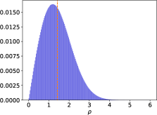
(a) Distribution of which Eq. (57) is the average.

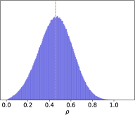
(b) Distribution of which Eq. (59) is the average.

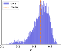
(c) Distribution of which Eq. (58) is the average.

Figure 14: Histogram data of various estimators of $\left\langle\rho\right\rangle$ for $N_{\mathrm{s}}=255$, $N_{\mathrm{t}}=72$, $\mu=0$ and $g^{-2}=1.0540$. The vertical axes show the relative number of hits per bin, with 200 bins used for each histogram. Note that all values of $\rho$ shown here are raw numerical data not in physical units.

For an easy comparison of our results with the analytic large-$N_{\mathrm{f}}$ solution we use $\rho_{0}=\left\langle\rho\right\rangle_{T=\mu=0}$ to set the scale. Unfortunately, it is difficult to obtain an accurate estimate for $\langle\rho\rangle$ in our simulations. In this appendix, we first explain the (statistical) problems with direct approaches to measure $\left\langle\rho\right\rangle$ and afterwards present our solution.

From a field theory perspective, the direct lattice estimator for $\left\langle\rho\right\rangle$ would be $\rho_{t,x}$ for any (fixed) point $(t,x)$ on the lattice. Now, $\rho_{t,x}$ should be homogeneous up to fluctuations and, hence, one can improve the statistics by combining the data from all estimators $\rho_{t,x}$ for all lattice points. Example data for this estimator can be seen in Fig. 14(a).

The final estimate for $\left\langle\rho\right\rangle$ would then read

$$\left\langle\rho\right\rangle\approx\left(\mathrm{mean}_{\tau}\circ\mathrm{mean}_{x}\circ\mathrm{mean}_{t}\circ\mathrm{abs}\right)\Delta_{t,x}^{(\tau)}\;,$$ (57)

where $\tau$ is the MC time, $\Delta_{t,x}^{(\tau)}$ the field value at site $(t,x)$ of the $\tau$’th configuration and $\mathrm{mean}_{\#}$ means averaging with respect to the respective subscript. In order to actually show the distribution from which the final estimates are calculated, we present (here and in the following) the histograms one obtains by stripping the means after the absolute values have been taken.

The histogram of the straightforward estimator shown in Fig. 14(a) is dominated by its broad variance (as is expected for a local estimator). More importantly, since the field $\theta$ is quasi-long-range, it requires many sweeps through the lattice to obtain a $\theta$-independent distribution of $\Delta$ like the ones depicted in Fig. 2. In fact, a typical configuration in the simulations is not distributed symmetrically around the origin but rather around some finite value $\Delta_{0}$. The center of the configurations moves slowly (in Monte Carlo time) around the origin in field space. For this reason, taking the modulus right in the beginning leads to a significant bias towards larger values in the estimator (57).

The broad variance mentioned above is a known statistical phenomenon in MC simulations and is usually cured by averaging over the spacetime lattice before taking the absolute value, schematically

$$\left\langle\rho\right\rangle\approx\left(\mathrm{mean}_{\tau}\circ\mathrm{abs}\circ\mathrm{mean}_{x}\circ\mathrm{mean}_{t}\right)\Delta_{t,x}^{(\tau)}\;.$$ (58)

This sharpens the distribution but is less well motivated from a field theory perspective. The choice (58) can be justified if there is spontaneous symmetry breaking and a small trigger is sufficient to align the values of the field on the lattice sites. In this case the absolute value does not change the result if we take the limits in the correct order, i.e. the spatial volume to infinity before removing the trigger. In the symmetric phase, on the other hand, already the spatial average should vanish in the thermodynamic limit and again taking the absolute value does not make a difference. Example distributions of this estimator are shown in Fig. 14(c). Note the different scales on the $x$ axes.

It may come as a surprise that there is a second peak visible that distorts the mean of this distribution. This is due to the fact that at any non-zero temperature there are contributions from inhomogeneous configurations, which average out over the lattice to a very good approximation, see also Fig. 11. While for these data the distortion might be mild, we are not willing to take the risk of severely underestimating the observable for scale setting.

In the present work, what is even more problematic is that long-range (quasi-periodic) inhomogeneities must not be averaged over the spatial direction before taking absolute values. But, since we have to improve statistics as much as possible we will compromise by using

$$\left\langle\rho\right\rangle\approx\left(\mathrm{mean}_{\tau}\circ\mathrm{mean}_{x}\circ\mathrm{abs}\circ\mathrm{mean}_{t}\right)\Delta_{t,x}^{(\tau)}\;,$$ (59)

where we, similarly as in the spatial correlation functions (37), first average over time.

As Fig. 14(b) indicates, this yields acceptable statistics while only using the assumption of temporal homogeneity which is a feature of all large-$N_{\mathrm{f}}$ results we know of and was checked to be valid in our MC data, see, for example, Fig. 4. One should note that this procedure does not work in the high-temperature regime as the distribution in this case approaches that of Eq. (57).

In future works other scale settings could be used and the corresponding results should be compared with those obtained in the present work. For example, the mass of the field $\rho(t,x)$ may serve as an energy scale. The drawback of choosing a scale different from the minimum of the effective potential $U_{\mathrm{eff}}(\rho)$ (at zero temperature and density) is that it is less straightforward to relate to the analytic results for large $N_{\mathrm{f}}$. In the large-$N_{\mathrm{f}}$ limit the field $\rho$ becomes infinitely heavy.

Appendix B Autocorrelation analysis

During our simulations, we had to tackle severe autocorrelations similar to those described in Lenz et al. (2020b). In this appendix we summarize our extensive analysis of autocorrelation functions (ACFs) of various lattice estimators and provide details on how we arrive at the conclusion that our qualitative statements are robust despite large autocorrelations for certain parameter regions.

B.1 Identifying autocorrelation scales in an example

To facilitate such a discussion it is useful to visualize the topography of the effective action of the theory. In the infinite volume and – less important for this argument – continuum case, Başar et al. (2009) found the general form of the saddle points of the effective action. The spatial profiles of the order parameter $\Delta$ are given as a continuous family with four parameters related to overall scale, amplitude and phase variations, and a phase offset which is tightly related to translations. The finite volume we work in subjects these self-consistent solutions to the imposed boundary conditions such that for some of these parameters only a discrete subset of allowed solutions yields saddle points in finite volume. This entails a ragged landscape of valleys with local minima of the effective action that are separated by ridges stemming from the finite-volume effects and melting in the infinite-volume limit. From the analytical results, we expect chiral–spiral-like local minima (including the degenerate one, i.e. the constant order parameter) to be most important and our simulations confirm this expectation.

The above discussion immediately suggests that there are three qualitatively different kinds of autocorrelations: Sampled configurations will typically tend to fluctuate around one local minimum correlated within this valley on a (MC-time) scale $\tau_{\mathrm{fluct}}$. During this process the reference chiral spiral will rotate the overall phase offset on a time scale $\tau_{\mathrm{U}(1)}$ which, for non-degenerate chiral spirals, is equivalent to translating this spiral. Eventually, the algorithm will climb (or tunnel through) a ridge and arrive in another valley on a time scale $\tau_{k_{\mathrm{max}}}$.

From these three time scales, $\tau_{\mathrm{U}(1)}$ is of minor importance to us because we carefully crafted all of our observables to respect the $\mathrm{U}(1)$ (and closely related translational) symmetry. From the notable exceptions Fig. 2 and Fig. 13, however, we learned that it is quite sizable but clearly under control as the almost-perfect circles of Fig. 2 illustrate.

The other autocorrelation scales can be clearly distinguished in Fig. 15. For one exemplary parameter set, the figure shows ACFs of $C_{\sigma\sigma}(x)$ for some randomly chosen lattice points $x$ as well as the average and the (local in MC-time separation) maximal autocorrelations obtained over all lattice points. The latter rather unconventional quantity can be considered as a worst-case scenario for autocorrelations in $C_{\sigma\sigma}$.

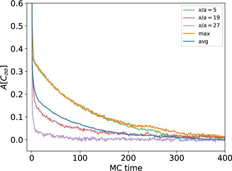
Figure 15: Autocorrelation functions for $C_{\sigma\sigma}(x)$ for three different $x$, a maximum over all $x$ and an average over all $x$ for $N_{\mathrm{f}}=2$, $N_{\mathrm{s}}=63$, $T/\rho_{0}\approx 0.09$, $\mu/\rho_{0}\approx 0.61$, $a\rho_{0}\approx 0.46$.

All of these are well described by an ansatz

$$A[C_{\sigma\sigma}](t)=be^{-t/\tau_{1}}+(1-b)e^{-t/\tau_{2}}\;,$$

where $b$, $\tau_{1}$ and $\tau_{2}$ are free parameters. While the detailed numbers obviously depend on the data set chosen for fitting, the orders of magnitudes are consistent (cf. Tab. 1).

Table 1: Fit parameters $b$, $\tau_{1}$ and $\tau_{2}$ for the autocorrelation function of $C_{\sigma\sigma}(x)$ for some values of $x$ as well as an average and a maximum over all $x$ (cf. Fig. 15).

	$b$	$\tau_{1}$	$\tau_{2}$
$x/a=5$	0.65	0.3	111.5
$x/a=19$	0.86	0.8	101.5
$x/a=27$	0.94	0.5	32.8
avg	0.79	0.6	87.0
max	0.66	0.9	125.5

In order to associate the two numerical values $\tau_{1}$ and $\tau_{2}$ with the mechanisms described above, we consider representative time evolutions on each time scale in Fig. 16. Fig. 16(a) shows the Fourier spectrum of $C_{\sigma\sigma}$ over $20\times\tau_{1}$ MC configurations where we conservatively use $\tau_{1}\approx 1$. It is clearly seen that there is a constant peak at $\nu_{\mathrm{max}}=3$, while the MC evolution produces small fluctuations around this reference configuration. We conclude that the small time scale for this parameter set is generated from fluctuations around one local minimum, i.e. $\tau_{\mathrm{fluct}}=\tau_{1}$.

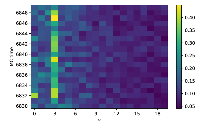
(a) Short MC time scales.

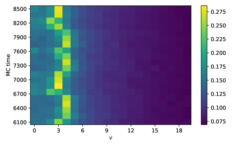
(b) Long MC time scales. The data was averaged over bins of size $\tau_{k_{\mathrm{max}}}=\tau_{2}\approx 126$.

Figure 16: MC timelines of the Fourier spectra of $C_{\sigma\sigma}$ for the same parameters as Fig. 15.

To probe the larger time scale, we show a MC-time window of $20\times\tau_{2}$ configurations in Fig. 16(b), where we conservatively estimated $\tau_{2}\approx 126$. For visual clarity, we averaged blocks of $\tau_{2}$ MC configurations which should be thought of as a coarse graining integrating out the high frequencies similar to an RG transformation. On this scale, the correlator spectra are smooth (due to the coarse graining) and sharp peaks and the MC evolution produces jumps in the dominant frequency $k_{\mathrm{max}}$. This finding relates the long time scale to $\tau_{k_{\mathrm{max}}}$ that was suggestively named after its effect of jumping between valleys changing $k_{\mathrm{max}}$. One should also stress that it is a non-trivial statement that 126 configurations tend to be rather coherent – again strengthening the association of $\tau_{2}$ with $\tau_{k_{\mathrm{max}}}$.

B.2 Analysis and reasoning about the rest of parameter space

The previous example indicates two important facts: Firstly, our choice of algorithmic parameters rendered $\tau_{\mathrm{fluct}}$ negligible while $\tau_{k_{\mathrm{max}}}$ is of considerable size. Secondly, besides $\tau_{k_{\mathrm{max}}}$ being large it is still under control in the sense that we have a statistically significant number of independent configurations $N_{\mathrm{MC}}/\tau_{k_{\mathrm{max}}}\approx 380$ even in the worst case discussed above. As the chosen parameter set is well inside the region of intermediate-scale inhomogeneous order we conclude from a statistically robust ensemble that our claims of intermediate-scale inhomogeneities without spontaneous symmetry breaking of any kind are robust with respect to autocorrelation effects. We checked for similar examples on all lattice sizes and lattice spacings.

However, the above example was taken from a moderate temperature region. As we confirmed in this study, at the $T=0$ line the system is critical which implies diverging correlation lengths – also in the MC-time evolution as is well known around practitioners Janke (2008). We therefore expected and a posteriori verified huge autocorrelations for temperatures close to zero. One should stress that this is a physical effect; it can likely be circumvented by an appropriately adapted algorithm but still bares physically relevant information. Still, for a small region of very low temperatures $\tau_{k_{\mathrm{max}}}$ can easily exceed our greatest efforts of up to $8\cdot 10^{4}$ configurations generated for some parameter sets. We therefore suggest to view the very-low-temperature results with a grain of salt quantitatively: They surely give a good impression of what phenomena to expect in the exceedingly large regions of space that are correlated for these temperatures but they might be quantitatively off due to autocorrelations suppressing the interference from subdominant local minima.

We remark that $\tau_{k_{\mathrm{max}}}$ has a clear tendency to decrease in the infinite-volume limit. This is the opposite behavior of what is typically found in symmetry-breaking systems and considered further evidence in support of the existence of a BKT phase and against spontaneous symmetry breaking, as was also mentioned in the main text.

The effect of larger flavor numbers is to reduce quantum fluctuations or, in the pictorial language from above, to deepen the valleys and grow the ridges. This effect is responsible for ultimately obtaining actual spontaneous symmetry breaking in the limit of infinite number of flavors. It also greatly enhances autocorrelations, particularly in suppressing jumps between different valleys. For $N_{\mathrm{f}}=8$ the temperatures necessary to clearly observe inhomogeneities on average and jumps in the dominant wave number during the MC evolution occur concurrently are higher than in the 2-flavor case. This strengthens our finding in this and previous papers Lenz et al. (2020a, b) that the convergence to mean-field behavior is quite rapid with the number of flavors. While technically this casts some doubt on the quantitative accuracy of the $N_{\mathrm{f}}=8$ data, we want to point out again that this is driven by physical properties of the system more than technical difficulties.

Finally, we want to share some thoughts on how to improve on the situation: Due to extensive analytical results about the effective action, we were able to obtain a clear picture of the cause of autocorrelations in this model. One can easily imagine algorithmic improvements leveraging this knowledge. As the local minima can be enumerated by their dominant wave number $k_{\mathrm{max}}$, local updates in Fourier space might suffice, e.g. local Metropolis-like updates or swapping of Fourier components. As the current updating scheme is very efficient to reduce some part of the autocorrelations, it would probably be advantageous to combine both kinds of updates into a single update step. Similar ideas are already used, e.g. Albandea et al. (2021). Another approach could be to constrain the simulations to a single sector and a posteriori combining the results into a weighted sum.

However, these approaches would be very specific and hardly generalizable to related problems, e.g. topological freezing in lattice QCD Allés et al. (1996). A modern approach that is agnostic of analytical knowledge, which is usually not as easily employed in more realistic theories, could be independence samplers from generative models, i.e. independently drawing the configurations from an efficient approximation of the probability distribution. Promising results in this direction were presented in Kanwar et al. (2020), where they overcame topological freezing in 1+1D $\mathrm{U}(1)$ gauge theory.

Appendix C On fermionic 4-point functions

We aim at relating the U_A(1)-invariant fermion $4$-point function (44) to the spatial correlation functions $C_{\sigma\sigma}$ and $C_{\sigma\pi}$ defined in Eq. (37). To find such a relation we exploit the following Dyson-Schwinger equations, which can be derived in analogy to Eq. (6):

$$\begin{aligned} \langle\bar{\psi}\psi(\boldmathe{x})\bar{\psi}\psi(\boldmathe{y})\rangle&=-\kappa^{2}\langle\sigma(\boldmathe{x})\sigma(\boldmathe{y})\rangle+\kappa\delta^{2}(\boldmathe{x}-\boldmathe{y})\;,\\ \langle\bar{\psi}\psi(\boldmathe{x})\bar{\psi}\gamma_{*}\psi(\boldmathe{y})\rangle&=\mathrm{i}\kappa^{2}\langle\sigma(\boldmathe{x})\pi(\boldmathe{y})\rangle\;,\\ \langle\bar{\psi}\gamma_{*}\psi(\boldmathe{x})\bar{\psi}\psi(\boldmathe{y})\rangle&=\mathrm{i}\kappa^{2}\langle\pi(\boldmathe{x})\sigma(\boldmathe{y})\rangle\;,\\ \langle\bar{\psi}\gamma_{*}\psi(\boldmathe{x})\bar{\psi}\gamma_{*}\psi(\boldmathe{y})\rangle&=\kappa^{2}\langle\pi(\boldmathe{x})\pi(\boldmathe{y})\rangle-\kappa\delta^{2}(\boldmathe{x}-\boldmathe{y})\;,\end{aligned}$$ (60)

wherein we used the abbreviation

$$\kappa=\frac{N_{\mathrm{f}}}{g^{2}}\,.$$ (61)

Recalling that $\Delta=\sigma+\mathrm{i}\pi$ we can write the invariant $4$-point function as

$$C_{\mathrm{4F}}(\boldmathe{x};\boldmathe{y})=-\kappa^{2}\langle\Delta^{*}(\boldmathe{x})\Delta(\boldmathe{y})\rangle+2\kappa\,\delta^{2}(\boldmathe{x})\;,$$ (62)

and the axial U_A(1) symmetry implies (cf. Eq. (38))

$$\langle\Delta^{*}(\boldmathe{x})\Delta(\boldmathe{y})\rangle=2\langle\sigma(\boldmathe{x})\sigma(\boldmathe{y})\rangle+2\mathrm{i}\langle\sigma(\boldmathe{x})\pi(\boldmathe{y})\rangle\;.$$ (63)

In analogy to the spatial correlation functions (37) for the condensate fields we introduced the spatial correlation function for the $N_{\mathrm{f}}$ Fermi fields on the lattice in Eq. (46). Inserting (63) into (62) we can relate (46) to (37) as follows:

$$C_{\mathrm{4F}}(x)=-2\kappa^{2}\left(C_{\sigma\sigma}(x)+\mathrm{i}\,C_{\sigma\pi}(x)\right)+2\kappa\delta(x)\;,$$ (64)

where on the lattice the spatial $\delta$ distribution on the right-hand side turns into the Kronecker symbol $\delta_{x,0}$.

Appendix D Parameters

Table 2: Lattice spacings for each set of $(N_{\mathrm{f}},N_{\mathrm{s}},g^{2})$. The right column contains the values of $N_{\mathrm{t}}$ at which the scale setting was performed and the asterisk on one value of $a\rho_{0}$ indicates that the given uncertainty was estimated by hand to be larger than the computed jackknife uncertainty due to small statistics.

$N_{\mathrm{f}}$	$N_{\mathrm{s}}=L/a$	$1/g^{2}$	$a\rho_{0}$	$N_{\mathrm{t}}$
$2$	$63$	1.0540	$0.45655\pm 0.00061$	$72$
$2$	$127$	1.0540	$0.45844\pm 0.00095$	$72$
$2$	$255$	1.0540	$0.4573\pm 0.0012$	$72$
$2$	$127$	1.3895	$0.1904\pm 0.0027$	$240$
$2$	$255$	1.8254	$0.08\pm 0.01^{*}$	$648$
$8$	$63$	5.1013	$0.41235\pm 0.00023$	$80$

In order to calculate the various phase diagrams we generated many ensembles characterized by the control parameters $(N_{\mathrm{f}},T,L,\mu)$ or $(N_{\mathrm{f}},N_{t},N_{s},\rho_{0}\mu)$, plus the four-Fermi coupling $g^{2}$ tuned to the required lattice spacing measured in units of $\rho_{0}=\langle\rho\rangle_{T=\mu=0}$. We summarize the lattice spacings corresponding to the different values of $N_{\mathrm{f}}$, $N_{\mathrm{s}}$ and $g^{2}$ in Tab. 2.

As explained in the main text, we used different initial conditions for the fields to deal with thermalization problems: We performed scans with Gaussian-distributed seeds with mean zero, a freeze-out from high temperatures to reduce thermalization times and a heat-up procedure from the lowest temperature to exclude any hysteresis effects from the freeze-out. We also used a homogeneous cold start, in the sense of setting the initial configuration to $\Delta({\boldmathe{x}})=1+\mathrm{i}$ for all $\boldmathe{x}$, at small $\mu$, where inhomogeneous configurations are suppressed. In Tab. 3 we collect the control parameters $N_{\mathrm{t}}$ and $\mu$ for which we generated ensembles in equilibrium for each of these methods. Notice that we use the same lattice spacings as in Tab. 2, which were determined via the freeze-out procedure, irrespective of the initial conditions.

Table 3: Parameter sets used in the simulations. Note that the uncertainty of $a\rho_{0}$ (from Tab. 2) propagates to the values of $\mu/\rho_{0}$, although we did not make this explicit for the sake of readability.

$N_{\mathrm{s}}=L/a$	$1/g^{2}$	$N_{\mathrm{t}}=1/Ta$	$\mu/\rho_{0}$
infinite-volume extrapolation $(N_{\mathrm{f}}=2$)
$63$	1.0540	2, 4, 6, 8, 10, 12, 16, 24, 32, 40, 48, 72	0, 0.0876, …, 1.3142
$127$	1.0540	2, 4, 6, 8, 10, 12, 16, 24, 36, 48, 72	0, 0.0873, …, 1.3088
$255$	1.0540	2, 4, 6, 8, 10, 12, 16, 24, 36, 48, 72	0, 0.0875, …, 1.3121
continuum extrapolation $(N_{\mathrm{f}}=2$)
$127$	1.3895	4, 6, 8, 10, 12, 16, 24, 36, 48, 72, 96, 144	0, 0.1050, …, 1.5756
$255$	1.8254	8, 12, 16, 24, 36, 48, 72, 96, 144	0, 0.1250, …, 1.8750
independent initial conditions ($N_{\mathrm{f}}=2$, for crosschecks)
$63$	1.0540	16, 24, 32, 40, 48, 56, 64, 80	0, 0.0876, …, 1.3142
$127$	1.0540	24, 32, 40, 48, 64, 80	0, 0.0873, …, 1.3088
$255$	1.0540	8, 16, 24, 32, 40, 48, 64, 80	0, 0.0875, …, 1.3121
$127$	1.3895	8, 16, 40, 48, 64, 80	0, 0.1050, …, 1.5756
$255$	1.8254	24, 32, 40, 48, 64	0, 0.1250, …, 1.8750
independent initial conditions ($N_{\mathrm{f}}=8$)
$63$	5.1013	4, 6, 8, 12, 16, 20, 24, 28, 32, 36, 40, 48, 56, 64, 80	0, 0.0970, …, 1.4551
heat-up initial conditions ($N_{\mathrm{f}}=2$, for checking hysteresis effects)
127	1.0540	16, 24, 36, 48, 72	0.4363, 0.8725, 1.3088
cold start ($N_{\mathrm{f}}=2$, small $\mu$)
63	1.0540	2, 4, 6, 8, 10, 12, 24, 48, 72	0, 0.0876, 0.1752

References

- Nambu and Jona-Lasinio (1961) Y. Nambu and G. Jona-Lasinio, Phys. Rev. 122, 345 (1961).
- Fermi (1934) E. Fermi, Z. Phys. 88, 161 (1934).
- Hill and Simmons (2003) C. T. Hill and E. H. Simmons, Phys. Rep. 381, 235 (2003), [Erratum: Phys.Rept. 390, 553 (2004)], arXiv:hep-ph/0203079 [hep-ph] .
- Miransky et al. (1989) V. A. Miransky, M. Tanabashi, and K. Yamawaki, Phys. Lett. B 221, 177 (1989).
- Thirring (1958) W. E. Thirring, Ann. Phys. 3, 91 (1958).
- Gross and Neveu (1974) D. J. Gross and A. Neveu, Phys. Rev. D 10, 3235 (1974).
- Campbell and Bishop (1982) D. K. Campbell and A. R. Bishop, Nucl. Phys. B 200, 297 (1982).
- Chodos and Minakata (1994) A. Chodos and H. Minakata, Phys. Lett. A 191, 39 (1994).
- Caldas (2011) H. Caldas, J. Stat. Mech. 2011, P10005 (2011), arXiv:1106.0948 [cond-mat] .
- Kuno (2019) Y. Kuno, Phys. Rev. B 99, 064105 (2019), arXiv:1811.01487 [cond-mat] .
- Thies and Urlichs (2005) M. Thies and K. Urlichs, Phys. Rev. D 72, 105008 (2005), arXiv:hep-th/0505024 .
- Ebert and Blaschke (2019) D. Ebert and D. Blaschke, Prog. Theor. Exp. Phys. 2019, 123I01 (2019), arXiv:1811.07109 [cond-mat] .
- Ebert et al. (2016) D. Ebert, K. G. Klimenko, P. B. Kolmakov, and V. C. Zhukovsky, Ann. Phys. 371, 254 (2016), arXiv:1509.08093 [cond-mat] .
- Liu (1999) W. V. Liu, Nucl. Phys. B 556, 563 (1999).
- Zhukovskii et al. (2001) V. C. Zhukovskii, K. G. Klimenko, V. V. Khudyakov, and D. Ebert, JETP Lett. 73, 121 (2001), arXiv:hep-th/0012256 .
- Thies (2004) M. Thies, Phys. Rev. D 69, 067703 (2004), arXiv:hep-th/0308164 .
- Schön and Thies (2000) V. Schön and M. Thies, Phys. Rev. D 62, 096002 (2000), arXiv:hep-th/0003195 .
- Schön and Thies (2001) V. Schön and M. Thies, (2001), arXiv:hep-th/0008175 .
- Thies (2006) M. Thies, J. Phys. A. 39, 12707 (2006), arXiv:hep-th/0601049 .
- Fulde and Ferrell (1964) P. Fulde and R. A. Ferrell, Phys. Rev. 135, A550 (1964).
- Larkin and Ovchinnikov (1964) A. I. Larkin and Y. N. Ovchinnikov, Zh. Eksp. Teor. Fiz. 47, 1136 (1964).
- Casalbuoni and Nardulli (2004) R. Casalbuoni and G. Nardulli, Rev. Mod. Phys. 76, 263 (2004), arXiv:hep-ph/0305069 .
- Bloch et al. (2008) I. Bloch, J. Dalibard, and W. Zwerger, Rev. Mod. Phys. 80, 885 (2008), arXiv:0704.3011 [cond-mat] .
- Lenz et al. (2020a) J. J. Lenz, L. Pannullo, M. Wagner, B. H. Wellegehausen, and A. Wipf, Phys. Rev. D 101, 094512 (2020a), arXiv:2004.00295 [hep-lat] .
- Lenz et al. (2020b) J. J. Lenz, L. Pannullo, M. Wagner, B. H. Wellegehausen, and A. Wipf, Phys. Rev. D 102, 114501 (2020b), arXiv:2007.08382 [hep-lat] .
- Bergner et al. (2008) G. Bergner, T. Kästner, S. Uhlmann, and A. Wipf, Ann. Phys. 323, 946 (2008), arXiv:0705.2212 [hep-lat] .
- Kästner et al. (2008) T. Kästner, G. Bergner, S. Uhlmann, A. Wipf, and C. Wozar, Phys. Rev. D 78, 095001 (2008), arXiv:0807.1905 [hep-lat] .
- Wellegehausen et al. (2017) B. H. Wellegehausen, D. Schmidt, and A. Wipf, Phys. Rev. D 96, 094504 (2017), arXiv:1708.01160 [hep-lat] .
- Lenz et al. (2019) J. J. Lenz, B. H. Wellegehausen, and A. Wipf, Phys. Rev. D 100, 054501 (2019), arXiv:1905.00137 [hep-lat] .
- Hands et al. (2020) S. Hands, M. Mesiti, and J. Worthy, Phys. Rev. D 102, 094502 (2020), arXiv:2009.02964 [hep-lat] .
- Başar et al. (2009) G. Başar, G. V. Dunne, and M. Thies, Phys. Rev. D 79, 105012 (2009), arXiv:0903.1868 [hep-th] .
- Landau and Lifshitz (1980) L. D. Landau and E. M. Lifshitz, Statistical Physics, 3rd ed. (Pergamon Press Ltd. Oxford, 1980).
- Mermin and Wagner (1966) N. D. Mermin and H. Wagner, Phys. Rev. Lett. 17, 1133 (1966), [Erratum: Phys. Rev. Lett. 17, 1307 (1966)].
- Hohenberg (1967) P. C. Hohenberg, Phys. Rev. 158, 383 (1967).
- Coleman (1973) S. Coleman, Commun. Math. Phys. 31, 259 (1973).
- Peierls (1934) R. Peierls, Helv. Phys. Acta 7, 81 (1934).
- Dashen et al. (1975) R. F. Dashen, S.-K. Ma, and R. Rajaraman, Phys. Rev. D 11, 1499 (1975).
- Berezinsky (1971) V. L. Berezinsky, Sov. Phys. JETP 32, 493 (1971).
- Kosterlitz and Thouless (1973) J. M. Kosterlitz and D. J. Thouless, J. Phys. C 6, 1181 (1973).
- Witten (1978) E. Witten, Nucl. Phys. B 145, 110 (1978).
- Bramwell and Holdsworth (1994) S. T. Bramwell and P. C. W. Holdsworth, Phys. Rev. B 49, 8811 (1994).
- Drell et al. (1976a) S. D. Drell, M. Weinstein, and S. Yankielowicz, Phys. Rev. D 14, 487 (1976a).
- Drell et al. (1976b) S. D. Drell, M. Weinstein, and S. Yankielowicz, Phys. Rev. D 14, 1627 (1976b).
- Andersen (2005) J. O. Andersen, (2005), arXiv:hep-th/0506261 .
- Stoll et al. (2021) J. Stoll, N. Zorbach, A. Koenigstein, M. J. Steil, and S. Rechenberger, (2021), arXiv:2108.10616 [hep-ph] .
- O’Raifeartaigh et al. (1986) L. O’Raifeartaigh, A. Wipf, and H. Yoneyama, Nucl. Phys. B 271, 653 (1986).
- Endrődi et al. (2021) G. Endrődi, T. G. Kovács, and G. Markó, Phys. Rev. Lett. 127, 232002 (2021), arXiv:2109.03668 [hep-lat] .
- Pisarski et al. (2020) R. D. Pisarski, A. M. Tsvelik, and S. Valgushev, Phys. Rev. D 102, 016015 (2020), arXiv:2005.10259 [hep-ph] .
- Horie and Nonaka (2021) K. Horie and C. Nonaka, PoS(LATTICE2021)150 (2021), arXiv:2112.02261 [hep-lat] .
- Janke (2008) W. Janke, in Computational Many-Particle Physics, Vol. 739, edited by H. Fehske, R. Schneider, and A. Weiße (Springer Berlin Heidelberg, Berlin, Heidelberg, 2008) pp. 79–140.
- Albandea et al. (2021) D. Albandea, P. Hernández, A. Ramos, and F. Romero-López, Eur. Phys. J. C 81, 873 (2021), arXiv:2106.14234 [hep-lat] .
- Allés et al. (1996) B. Allés, G. Boyd, M. D’Elia, A. Di Giacomo, and E. Vicari, Phys. Lett. B 389, 107 (1996), arXiv:hep-lat/9607049 .
- Kanwar et al. (2020) G. Kanwar, M. S. Albergo, D. Boyda, K. Cranmer, D. C. Hackett, S. Racanière, D. J. Rezende, and P. E. Shanahan, Phys. Rev. Lett. 125, 121601 (2020), arXiv:2003.06413 [hep-lat] .