Quantum Spectral Curve for $AdS_{3}/CFT_{2}$: a proposal

Abstract

We conjecture the Quantum Spectral Curve equations for string theory on $AdS_{3}\times S^{3}\times T^{4}$ with RR charge and its $\text{CFT}_{2}$ dual. We show that in the large-length regime, under additional mild assumptions, the QSC reproduces the Asymptotic Bethe Ansatz equations for the massive sector of the theory, including the exact dressing phases found in the literature. The structure of the QSC shares many similarities with the previously known $\text{AdS}_{5}$ and $\text{AdS}_{4}$ cases, but contains a critical new feature – the branch cuts are no longer quadratic. Nevertheless, we show that much of the QSC analysis can be suitably generalised producing a self-consistent system of equations. While further tests are necessary, particularly outside the massive sector, the simplicity and self-consistency of our construction suggests the completeness of the QSC.

1 Introduction

The Quantum Spectral Curve (QSC) has become an indispensable tool of precision spectroscopy in $\text{AdS}_{5}/\text{CFT}_{4}$ and $\text{AdS}_{4}/\text{CFT}_{3}$ holographic models Gromov:2013pga ; Gromov:2014caa ; Gromov:2014bva ; Gromov:2015wca ; Gromov:2015dfa ; Gromov:2015vua ; Marboe:2014gma ; Marboe:2018ugv ; Alfimov:2014bwa ; Alfimov:2020obh ; Alfimov:2018cms ; Gromov:2016rrp ; Cavaglia:2014exa ; Bombardelli:2017vhk ; Gromov:2014eha ; Anselmetti:2015mda ; Bombardelli:2018bqz ; Cavaglia:2018lxi ; Grabner:2020nis ; Cavaglia:2021bnz . For a review on the QSC, see Gromov:2017blm . In this paper, we shall take a step towards extending this powerful method to the spectral problem in another important holographic duality, namely planar $\text{AdS}_{3}/\text{CFT}_{2}$.

It is believed that $\text{AdS}_{3}/\text{CFT}_{2}$ dual pairs with 8+8 supersymmetries are integrable Babichenko:2009dk ; OhlssonSax:2011ms ; Cagnazzo:2012se . This is the maximal amount of supersymmetry that is allowed for string theory backgrounds of the form $\text{AdS}_{3}\times\mathcal{M}_{7}$, with ${\cal M}_{7}=\mathrm{S}^{3}\times\mathrm{T}^{4}$ or $\mathcal{M}_{7}=\mathrm{S}^{3}\times\mathrm{S}^{3}\times\mathrm{S}^{1}$. The symmetries of these two backgrounds are respectively the small and large $(4,4)$ superconformal symmetries, whose Lie sub-algebras are $\mathrm{psu}(1,1|2)^{2}$ and $\mathrm{d}(2,1;\alpha)^{2}$. The exact S matrices can be found by imposing compatibility with the (centrally extended) vacuum-preserving symmetry algebras of the two theories Borsato:2012ud ; Borsato:2013qpa ; Borsato:2014exa ; Borsato:2014hja ; Lloyd:2014bsa ; Borsato:2015mma , much like what can be done in higher-dimensional cases Beisert:2005tm . In this paper, we will focus on string theory on $\text{AdS}_{3}\times\mathrm{S}^{3}\times\mathrm{T}^{4}$ supported by R-R charge.

An important difference between these theories and higher-dimensional integrable string backgrounds is the presence of massless excitations in the worldsheet theory, in addition to the more familiar massive ones. The resulting integrable 2-to-2 S matrix breaks up into independent pieces for the scattering of massless/massless, massive/massive and mixed mass excitations. Expressed in terms of Zhukovsky variables, the S matrices resemble those of higher-dimensional integrable holographic theories, with the mass entering through the shortening conditions. This resemblance is particularly striking in the case of massive excitations Babichenko:2009dk ; Borsato:2013qpa , where in the weak-coupling limit the Bethe Equations (BEs) reduce to those of a homogeneous nearest-neighbour $\mathrm{psu}(1,1|2)\times\mathrm{psu}(1,1|2)$ spin-chain, with the two factors only connected by the level-matching condition. Away from the weak-coupling limit, the BEs for each $\mathrm{psu}(1,1|2)$ wing bear a striking similarity to the corresponding part of the $\mathrm{psu}(2,2|4)$ BEs of $\text{AdS}_{5}/\text{CFT}_{4}$. These observations suggest that (at least a part of) the $\text{AdS}_{3}/\text{CFT}_{2}$ Q-system can be constructed using two sets of $\mathrm{psu}(1,1|2)$ Q-functions, one for each wing, and coupling them together in a way that is consistent with the crossing. The Q-system is an important part of any known QSC Bombardelli:2017vhk ; Gromov:2014caa . In this paper, instead of deriving the QSC following a long route from TBA equations, we use the Q-system as a starting point supplying it with the analyticity properties following closely the previously known cases. However, fairly quickly we realise that one of the analyticity assumptions must be relaxed in our case – namely we no longer assume the square-root type of singularity near the branch points. This new feature is inherently connected with the properties of the dressing factors of Borsato:2014hja ; Lloyd:2014bsa ; Borsato:2015mma .

Each S matrix block comes with a dressing factor which is not fixed by symmetry requirements. Dressing factors satisfy crossing equations Borsato:2014hja ; Lloyd:2014bsa ; Borsato:2015mma that follow from the Hopf algebra structure of the theory Janik:2006dc ; Gomez:2006va ; Plefka:2006ze . In the case of string theory on $\text{AdS}_{3}\times\mathrm{S}^{3}\times\mathrm{T}^{4}$ supported by R-R charge only, dressing factors which solve these crossing equations have been found Borsato:2013hoa ; Borsato:2016kbm . There are two independent dressing phases that enter the massive S matrix, corresponding to either scattering excitations in the same $\mathrm{psu}(1,1|2)$ wing or in different wings. Their sum is equal to (twice) the Beisert-Eden-Staudacher (BES) phase Beisert:2006ez , while their difference is a new phase, which appears only at the so-called Hernandez-Lopez order Beccaria:2012kb . The relative simplicity of this latter factor is related to the fact that boundstates in the theory can only be made from massive constituent excitations from the same $\mathrm{psu}(1,1|2)$ wing. As with all solutions of crossing equations, there is potential for CDD ambiguities due to homogeneous solutions of crossing. The absence of such additional factors was demonstrated in OhlssonSax:2019nlj , where it was shown that the proposed dressing factors have exactly the required Dorey-Hofman-Maldacena (DHM) double poles and zeros Dorey:2007xn .

In the case of massive modes, crossing maps the two $\mathrm{psu}(1,1|2)$ wings into one another. This suggest that, as a consequence of crossing, the two copies of the $\mathrm{psu}(1,1|2)$ Q-systems should be related by a suitable analytic continuation. Analogous gluing conditions, which can be traced back to crossing, are known to exist in the $\text{AdS}_{5}/\text{CFT}_{4}$ and $\text{AdS}_{4}/\text{CFT}_{3}$ QSC and are needed in addition to the QQ-relations to constrain the system to a closed system of equations, which can be treated analytically Gromov:2015vua ; Marboe:2014gma in some limits and by means of numerical analysis Gromov:2015wca in general. Furthermore, the simple gluing of the Q-functions can be shown Gromov:2014caa ; Bombardelli:2017vhk to produce a rather involved expression for the BES dressing phase when considering the large-volume solution.

While a number of ingredients for the current construction are borrowed from the known cases, the new type of near-branch point singularity is a crucial novel ingredient. As a test of our proposal we demonstrated how the ABA equations for the massive sector are precisely reproduced in the large-length limit including the dressing phases. In these considerations, we had to make an additional simplifying assumption about the monodromy of $\mu$-function in the asymptotic limit, which we have not managed to prove. At the same time, we only reproduced the massive sector equations, which suggests that removing this assumption could revive all the massless degrees of freedom, but we leave this question for future work. Another important direction is to verify the completeness of our system of equations by solving it either numerically as in Gromov:2015wca or in a near BPS limits like in Gromov:2014bva ; Gromov:2014eha .

An intuitive way in which to understand the effect of massless modes is that the massless dispersion relation can be viewed in an approximate sense as the large coupling limit of the massive one, as long as the particle momentum is kept fixed. In the QSC formalism, the coupling usually controls the distance between the cuts in the rescaled spectral parameter $u/g$. As a result, in the zero mass limit, one might expect this to lead to a number of quadratic cuts collapsing on top of one another. This suggests that, in models with massless modes, the QSC may have a more general singularity structure near the branch points, rather than the conventional square root behaviour seen in higher-dimensional cases. We also expect the analyticity to be simplified in the purely massless sector by employing the pseudo-relativistic variable of Fontanella:2019baq ; Fontanella:2019ury .

In fact, the assumption of a square-root singularity is over-restrictive in $\text{AdS}_{3}$ because it gives rise to a new algebraic constraint on the Q-functions in addition to the QQ-relations. In turn, such a condition collapses the two wings of Q-functions into one, likely leading to drastically simpler analytic properties such as those seen in the Hubbard model  Cavaglia:2015nta , based on a single $su(2|2)$ symmetry.

The rest of the paper is organised as follows. In section 2, we collect pre-existing results on integrability for the AdS₃/CFT₂ duality, which will inspire our conjecture, and describe the algebraic structure of the Q-system for $psu(1,1|2)$. Section 3 presents our main proposal for the Quantum Spectral Curve, and describes the unique features of these equations as compared to the previous cases. In section 2.1, we study the large-volume limit of these equations, reproducing precisely the full Asymptotic Bethe Ansatz for massive modes. Finally, we present our conclusions and discuss some future directions. The paper also contains three appendices collecting some notations and technical details.

Note added: The work described here begun before the epidemic. Shortly after the first wave was coming to an end in Europe, we concluded that the large-length limit was incompatible with square-root cuts as described in section 4.3.1. During the recent “Integrability in Lower Dimensional AdS/CFT” online workshop we learnt that Simon Ekhammar and Dima Volin had also independently come to a similar conclusion. We are grateful to Dima and Simon for informing us of their findings and coordinating on the release date of the manuscripts to the arXiv. Motivated by these discussions, we revisited our construction and found that relaxing the branch-cut condition allows for a consistent definition of the QSC together with a large-length limit that reproduces the all-loop massive ABA equations found in the literature. Our proposal for the QSC seems to be fully consistent with the one published simultaneously in Ekhammar:2021pys .

Note added in v3: In the published version of this article we present a proposal for the QSC, whose large-volume solution involves the Riemann-Hilbert problem (4.46). In section 4.3.2, the solution to these equations is written in terms of $\chi(u,v)$ functions related to the dressing phases proposed in Borsato:2013hoa . These functions satisfy the correct discontinuity equations (4.46), but – upon closer inspection – they have an additional branch point at $u\sim\infty$. This extra branch point cancels in the full dressing phase of Borsato:2013hoa , but its presence in the building block $\chi^{-}(u,v)$ is incompatible with the proposed analyticity properties of the QSC. Thus, the claim that our construction reproduces the dressing phases of Borsato:2013hoa should be revised.
After the publication of this paper, a modified proposal for the dressing phases was made in Frolov:2021fmj , for which the extra branch point is absent from $\chi^{-}(u,v)$. We believe that these modified phases have a very good chance of arising naturally from our QSC in the large volume limit, at least for the massive-massive case, which would give extra supporting evidence for our construction and at the same time for the conjectured form of the dressing phases. A detailed analysis will be presented elsewhere (for a preliminary discussion see andreatalk ).
The remainder of this arXiv version reproduces in full the published article. We emphasize that our proposal for the QSC remains unmodifed, and the only change in the large-volume analysis comes in the explicit form of $\chi^{-}$.

2 Data on the AdS₃/CFT₂ integrable system

In this section we assemble together the known facts about the AdS₃/CFT₂ integrable system. This includes the asymptotic Bethe ansatz for massive modes, classical algebraic curve and the $psu(1,1|2)$ Q-system.

2.1 Asymptotic Bethe Ansatz

The massive Asymptotic Bethe Ansatz (ABA) equations which we will be referring to are those presented in Borsato:2013qpa . The symmetry controlling the Bethe equations is $\mathrm{psu}(1,1|2)^{2}$. Each copy of $\mathrm{psu}(1,1|2)$ has associated one momentum carrying root and two auxiliary roots. These are called $x,y_{1}$ and $y_{3}$ for one copy of $\mathrm{psu}(1,1|2)$ and $\bar{x},y_{\bar{1}}$ and $y_{\bar{3}}$, respectively, for the other copy. The explicit form of the BEs is:

$$1 = \prod_{j=1}^{K_{2}}\frac{y_{1,k}-x_{j}^{+}}{y_{1,k}-x_{j}^{-}}\prod_{j=1}^{K_{\bar{2}}}\frac{1-\frac{1}{y_{1,k}\bar{x}_{j}^{-}}}{1-\frac{1}{y_{1,k}\bar{x}_{j}^{+}}},$$

$$\bigg{(}\frac{x_{k}^{+}}{x_{k}^{-}}\bigg{)}^{L} = \prod_{j\neq k}^{K_{2}}\frac{x_{k}^{+}-x_{j}^{-}}{x_{k}^{-}-x_{j}^{+}}\frac{1-\frac{1}{x_{k}^{+}x_{j}^{-}}}{1-\frac{1}{x_{k}^{-}x_{j}^{+}}}\sigma^{2}(x_{k},x_{j})\prod_{j=1}^{K_{1}}\frac{x_{k}^{-}-y_{1,j}}{x_{k}^{+}-y_{1,j}}\prod_{j=1}^{K_{3}}\frac{x_{k}^{-}-y_{3,j}}{x_{k}^{+}-y_{3,j}}$$

$$\times\prod_{j=1}^{K_{\bar{2}}}\frac{1-\frac{1}{x_{k}^{+}\bar{x}_{j}^{+}}}{1-\frac{1}{x_{k}^{-}\bar{x}_{j}^{-}}}\frac{1-\frac{1}{x_{k}^{+}\bar{x}_{j}^{-}}}{1-\frac{1}{x_{k}^{-}\bar{x}_{j}^{+}}}\tilde{\sigma}^{2}(x_{k},\bar{x}_{j})\prod_{j=1}^{K_{\bar{1}}}\frac{1-\frac{1}{x_{k}^{-}y_{\bar{1},j}}}{1-\frac{1}{x_{k}^{+}y_{\bar{1},j}}}\prod_{j=1}^{K_{\bar{3}}}\frac{1-\frac{1}{x_{k}^{-}y_{\bar{3},j}}}{1-\frac{1}{x_{k}^{+}y_{\bar{3},j}}},$$

$$1 = \prod_{j=1}^{K_{2}}\frac{y_{3,k}-x_{j}^{+}}{y_{3,k}-x_{j}^{-}}\prod_{j=1}^{K_{\bar{2}}}\frac{1-\frac{1}{y_{3,k}\bar{x}_{j}^{-}}}{1-\frac{1}{y_{3,k}\bar{x}_{j}^{+}}},$$ (2.1)

$$1 = \prod_{j=1}^{K_{\bar{2}}}\frac{y_{\bar{1},k}-\bar{x}_{j}^{-}}{y_{\bar{1},k}-\bar{x}_{j}^{+}}\prod_{j=1}^{K_{2}}\frac{1-\frac{1}{y_{\bar{1},k}x_{j}^{+}}}{1-\frac{1}{y_{\bar{1},k}x_{j}^{-}}},$$

$$\bigg{(}\frac{\bar{x}_{k}^{+}}{\bar{x}_{k}^{-}}\bigg{)}^{L} = \prod_{j\neq k}^{K_{\bar{2}}}\frac{\bar{x}_{k}^{-}-\bar{x}_{j}^{+}}{\bar{x}_{k}^{+}-\bar{x}_{j}^{-}}\frac{1-\frac{1}{\bar{x}_{k}^{+}\bar{x}_{j}^{-}}}{1-\frac{1}{\bar{x}_{k}^{-}\bar{x}_{j}^{+}}}\sigma^{2}(\bar{x}_{k},\bar{x}_{j})\prod_{j=1}^{K_{\bar{1}}}\frac{\bar{x}_{k}^{+}-y_{\bar{1},j}}{\bar{x}_{k}^{-}-y_{\bar{1},j}}\prod_{j=1}^{K_{\bar{3}}}\frac{\bar{x}_{k}^{+}-y_{\bar{3},j}}{\bar{x}_{k}^{-}-y_{\bar{3},j}}$$

$$\times\prod_{j=1}^{K_{2}}\frac{1-\frac{1}{\bar{x}_{k}^{-}x_{j}^{-}}}{1-\frac{1}{\bar{x}_{k}^{+}x_{j}^{+}}}\frac{1-\frac{1}{\bar{x}_{k}^{+}x_{j}^{-}}}{1-\frac{1}{\bar{x}_{k}^{-}x_{j}^{+}}}\tilde{\sigma}^{2}(\bar{x}_{k},x_{j})\prod_{j=1}^{K_{1}}\frac{1-\frac{1}{\bar{x}_{k}^{+}y_{1,j}}}{1-\frac{1}{\bar{x}_{k}^{-}y_{1,j}}}\prod_{j=1}^{K_{3}}\frac{1-\frac{1}{\bar{x}_{k}^{+}y_{3,j}}}{1-\frac{1}{\bar{x}_{k}^{-}y_{3,j}}},$$

$$1 = \prod_{j=1}^{K_{\bar{2}}}\frac{y_{\bar{3},k}-\bar{x}_{j}^{-}}{y_{\bar{3},k}-\bar{x}_{j}^{+}}\prod_{j=1}^{K_{2}}\frac{1-\frac{1}{y_{\bar{3},k}x_{j}^{+}}}{1-\frac{1}{y_{\bar{3},k}x_{j}^{-}}}.$$ (2.2)

The Bethe equations are written in the grading illustrated in Fig. 1.

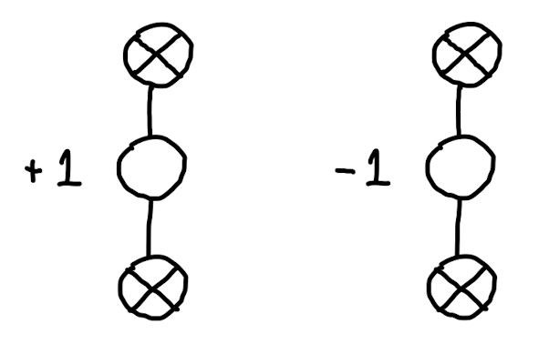
Figure 1: Grading used in the Asymptotic Bethe equations.

The massless modes will not be included in our analysis, and they do not feature anywhere in the Bethe equations we write. There is a further level-matching constraint on the solutions to the Bethe equations, in the form of

$$1=\prod_{j=1}^{K_{2}}\frac{x_{j}^{+}}{x_{j}^{-}}\prod_{j=1}^{K_{\bar{2}}}\frac{\bar{x}_{j}^{+}}{\bar{x}_{j}^{-}}$$ (2.3)

(once more disregarding massless modes). The Zhukovsky variables satisfy the familiar constraint given by (suppressing the particle index)

$$x^{+}+\frac{1}{x^{+}}-x^{-}-\frac{1}{x^{-}}=\frac{i}{h},\qquad\frac{x^{+}}{x^{-}}=e^{ip},$$ (2.4)

where $h$ is the coupling constant of the theory and $p$ is the particle momentum. The same holds for the barred variables. The dispersion relation that gives the energy of a particle of momentum $p$ reads

$$E(p)=\sqrt{1+16\,h^{2}\sin^{2}\frac{p}{2}},$$ (2.5)

and the anomalous dimension of the state associated to a solution of the ABA is given by

$$\delta\Delta\equiv\gamma=2h\sum_{k=1}^{K_{2}}\left(\frac{i}{x_{k}^{+}}-\frac{i}{x_{k}^{-}}\right)+2h\sum_{j=1}^{K_{\bar{2}}}\left(\frac{i}{\bar{x}_{j}^{+}}-\frac{i}{\bar{x}_{j}^{-}}\right).$$ (2.6)

The explicit form of the dressing phases from Borsato:2013hoa is given by

$$\sigma(p_{1},p_{2})=\mathrm{e}^{i\theta(p_{1},p_{2})},\qquad\tilde{\sigma}(p_{1},p_{2})=\mathrm{e}^{i\tilde{\theta}(p_{1},p_{2})},$$ (2.7)

with the familiar splitting

$$\theta(p_{1},p_{2})=\chi(x_{1}^{+},x_{2}^{+})+\chi(x_{1}^{-},x_{2}^{-})-\chi(x_{1}^{+},x_{2}^{-})-\chi(x_{1}^{-},x_{2}^{+}),$$ (2.8)

with similar expressions for $\tilde{\sigma}$. The individual blocks read

$$\chi(x,y)=\chi^{\mbox{\scriptsize BES}}(x,y)-\frac{1}{2}\Big{[}\chi^{\mbox{\scriptsize HL}}(x,y)-\chi^{-}(x,y)\Big{]},$$ (2.9)

$$\tilde{\chi}(x,y)=\chi^{\mbox{\scriptsize BES}}(x,y)-\frac{1}{2}\Big{[}\chi^{\mbox{\scriptsize HL}}(x,y)+\chi^{-}(x,y)\Big{]}.$$

The part denoted by BES is the Beisert-Eden-Staudacher Beisert:2006ez dressing phase - its expression can be found reproduced in the review Vieira:2010kb . The same holds for the HL part, referring to the Hernandez-Lopez phase Hernandez:2006tk

$$\chi^{{\rm HL}}(x,y)=\Bigg{(}\int_{C^{+}}-\int_{C^{-}}\Bigg{)}\frac{dw}{4\pi}\frac{1}{x-w}\Big{[}\log(y-w)-\log(y-\frac{1}{w})\Big{]}.$$ (2.10)

The new ingredient which was constructed in Borsato:2013hoa is given by

$$\chi^{-}(x,y)=\Bigg{(}\int_{C^{+}}-\int_{C^{-}}\Bigg{)}\frac{dw}{8\pi}\frac{1}{x-w}\log\Big{[}(y-w)\Big{(}1-\frac{1}{yw}\Big{)}\Big{]}-x\leftrightarrow y,$$ (2.11)

where the contours $C^{\pm}$ denote the upper (resp., lower) half semicircle in the complex $w$-plane, both running anti-clockwise. These expressions are valid in the physical region $|x|>1,|y|>1$. The notation $\chi^{-}$ is commonly used in the $\text{AdS}_{3}$ literature for this portion of the phase. The minus sign should not be confused with a shift in the spectral parameter - as will otherwise always be meant in this paper.

Since we will be merely concerned with the massive modes, it is expected that the Asymptotic Bethe equations which we have written above should be valid exactly in the coupling $h$ but only asymptotically in the length $L$. In other words, wrapping corrections are expected to be exponentially suppressed Bajnok:2010ke . This situation would be rather different were we to include massless modes, whose impact on the TBA is not exponentially suppressed - they are expected to be polynomially suppressed in the presence of mixed massive-massless interactions Abbott:2020jaa , or require exact solutions as in the case of the conformal TBA of Bombardelli:2018jkj ; Fontanella:2019ury (see also Abbott:2015pps ; Dei:2018jyj ).

Notice also that $4h$ gives the size of the branch cut which goes to zero at weak coupling. Since all interaction between the two $\mathrm{psu}(1,1|2)$ wings go through the branch-cut, the two wings become completely decoupled in the limit of small coupling constant $h\rightarrow 0$, except for the level-matching condition.

2.2 Main features of the classical curve

The Quantum Spectral Curve is a quantum version of the classical curve, which thus contains crucial structural hints. We shall from now on denote with un-dotted/dotted indices the variables pertaining to the first/second wing, respectively, of the Dynkin diagram – corresponding to the first/second copy of $\mathrm{psu}(1,1|2)$.

Here we present a short description of some aspects of the algebraic curve describing the integrability of classical solutions of string theory on $AdS_{3}\times S^{3}\times T^{4}$, following the discussion in Babichenko:2014yaa . This description is based on 4+4 quasimomenta, associated to the fundamental representations of the two $\mathrm{psu}(1,1|2)$’s. They will be denoted by $(p_{1}^{A},p_{2}^{A},p_{1}^{S},p_{2}^{S})$ and $(p_{\dot{1}}^{A},p_{\dot{2}}^{A},p_{\dot{1}}^{S},p_{\dot{2}}^{S})$. Each quasimomentum naturally parametrises motion in one of the factors of the target space, which is marked by the superscripts $A$, $S$ for $AdS_{3}$ and $S^{3}$, respectively. They are very important quantities which are expected to arise in a WKB-type approximation of the Q-functions in the classical limit of the quantum spectral curve.

The $p$’s are naturally seen as functions of the Zhukovsky variables, and contain the symmetry charges of the solution in their asymptotics:

$$\left(\begin{array}[]{c}p_{1}^{A}\\ p_{2}^{A}\\ p_{1}^{S}\\ p_{2}^{S}\end{array}\right) \simeq \frac{1}{2hx}\left(\begin{array}[]{c}-\Delta-S-\hat{B}\\ +\Delta+S-\hat{B}\\ -J-K-\hat{B}\\ +J+K-\hat{B}\end{array}\right)=\frac{1}{2hx}\left(\begin{array}[]{c}-\gamma-2K_{1}-L\\ +\gamma+2K_{3}+L\\ -2K_{1}+2K_{2}-L\\ -2K_{2}+2K_{3}+L\end{array}\right)\;,$$ (2.24)

$$\left(\begin{array}[]{c}p_{\dot{1}}^{A}\\ p_{\dot{2}}^{A}\\ p_{\dot{1}}^{S}\\ p_{\dot{2}}^{S}\end{array}\right) \simeq \frac{1}{2hx}\left(\begin{array}[]{c}+\Delta-S-\check{B}\\ -\Delta+S-\check{B}\\ +J-K-\check{B}\\ -J+K-\check{B}\end{array}\right)=\frac{1}{2hx}\left(\begin{array}[]{c}+\gamma-2K_{\dot{1}}+2K_{\dot{2}}+L\\ -\gamma-2K_{\dot{2}}+2K_{\dot{3}}-L\\ -2K_{\dot{1}}+L\\ 2K_{\dot{3}}-L\end{array}\right),$$ (2.37)

where on the rhs we used the explicit expression of the charges in terms of Bethe roots numbers. Finally, the classical curve tells us how the quasimomenta in the two wings are related. In particular, for the quasimomenta describing motion in $AdS_{3}$, the relation is extremely simple and consists in analytic continuation

$$p_{a}^{A}\left(\frac{1}{x}\right)=p_{\dot{a}}^{A}(x),\;\;a=1,2\,,$$ (2.38)

as described in equations (7.13) and (7.38) of Babichenko:2009dk . We will lift this property to the quantum case.

2.3 Algebra of the $\mathrm{psu}(1,1|2)$ Q-system

The sets of functional relations between the Q-functions (known as Q-systems) take a universal form depending only on the symmetry algebra of the integrable system. Since our model contains two copies of $\mathrm{psu}(1,1|2)$, important input for our construction comes from the structure of QQ relations for this algebra.

The $\mathrm{psu}(1,1|2)$ Q-system contains $16$ independent Q-functions depending on the spectral parameter $u$. They can be labelled as $Q_{A|I}$, where $A$, $I$ are completely anti-symmetric strings of indices made from $\left\{1,2\right\}$

$$A\,,I\in\left\{\emptyset,1,2,(12)\right\}\,,$$ (2.39)

interrelated by the QQ relations

$$Q_{aA|I}Q_{A|Ii} = Q_{aA|Ii}^{+}Q_{A|I}^{-}-Q_{aA|Ii}^{-}Q_{A|I}^{+}\,,$$ (2.40)

$$Q_{12|I}Q_{\emptyset|I} = Q_{1|I}^{+}Q_{2|I}^{-}-Q_{1|I}^{-}Q_{2|I}^{+}\,,$$ (2.41)

$$Q_{A|12}Q_{A|\emptyset} = Q_{A|1}^{+}Q_{A|2}^{-}-Q_{A|1}^{-}Q_{A|2}^{+}\,,$$ (2.42)

where $a,i\in\left\{1,2\right\}$ are single indices, and $A$, $I$ are anti-symmetric multi-indices defined above. The first type of relation (2.40) is usually called fermionic, and the remaining two bosonic. In these equations, we are using the notation adopted in the whole paper for shifts in the spectral parameter $u$: for any function $g$,

$$g^{[\pm n]}(u)\equiv g(u\pm\tfrac{in}{2})\,,\qquad\qquad g^{\pm}(u)\equiv g^{[\pm 1]}(u).$$ (2.43)

In our proposal, the QSC will contain two copies of these relations, which we will denote by distinguishing between dotted and undotted indices (giving us 16+16 Q-functions). In this section, we focus on one wing, and elaborate on some consequences of (2.40)-(2.42).

We will make a simple special choice for the Q-functions with the extremal combinations of indices:

$$Q_{\emptyset|\emptyset}=Q_{12|12}=1,$$ (2.44)

which is analogous to the choice made in the other known QSC cases. Notice that the Q-system has several symmetries, and in particular we are free to set $Q_{\emptyset|\emptyset}=1$ through an overall normalisation. The further, nontrivial algebraic assumption underlying (2.44) is that $Q_{12|12}(u)/Q_{\emptyset|\emptyset}(u)$ is an $i$-periodic function of $u$. Once we have this periodicity property, the analytic properties of Q-functions we will discuss in the next sections imply that $Q_{12|12}/Q_{\emptyset|\emptyset}$ should be a constant, which we are free to normalise to one using the symmetries of the Q-system. In quantum spin chains, the periodicity $1=\frac{Q_{12|12}^{+}Q_{\emptyset|\emptyset}^{-}}{Q_{12|12}^{-}Q_{\emptyset|\emptyset}^{+}}$ can be traced to the quantum transfer matrix having a unit determinant. It is also expected that such condition reflects the projectivity of the algebra $\mathrm{psu}(1,1|2)$. In particular, as discussed in Gromov:2014caa , it implements a zero-charge constraint for the quantum numbers, which enter the asymptotics of Q-functions in the way described in the next section. For these reasons, from now on we assume the validity of (2.44), which so far seems fully consistent with the description of the $AdS_{3}$ integrable system.

We will adopt a special notation for some of the Q-functions,

$${\bf Q}_{k}\equiv Q_{\emptyset|k},\;\;\;{\bf P}_{a}\equiv Q_{a|\emptyset},\;\;\;{\bf Q}^{k}\equiv\epsilon^{kl}Q_{12|l},\;\;\;{\bf P}^{a}\equiv\epsilon^{ab}Q_{b|12},$$ (2.45)

as well as $Q^{a|i}\equiv\epsilon^{ab}\epsilon^{ij}Q_{b|j}$. Explicitly,

$$Q^{a|i}=\left(\begin{array}[]{cc}Q_{2|2}&-Q_{2|1}\\ -Q_{1|2}&Q_{1|1}\end{array}\right),$$ (2.46)

such that

$$Q_{a|i}Q^{b|i}=\delta_{a}^{b},\;\;\;\;Q_{a|i}Q^{a|j}=\delta_{i}^{j},$$ (2.47)

due to the unimodularity property

$$\text{det}\left(Q_{a|i}\right)=1,$$ (2.48)

which is a consequence of the Q-system with the boundary conditions (2.44). Let us write explicitly some of the fermionic equations, which will be used extensively,

$$Q_{a|i}^{+}-Q_{a|i}^{-}={\bf P}_{a}{\bf Q}_{i},$$ (2.49)

together with $Q_{a|i}^{-}-Q_{a|i}^{+}=Q_{12|i}Q_{a|12}$, which can be rewritten in Hodge-dual notation as

$$Q^{a|i\;+}-Q^{a|i\;-}=-{\bf P}^{a}{\bf Q}^{i}.$$ (2.50)

Further useful consequences of the QQ relations are:

$${\bf P}_{a}{\bf P}^{a}={\bf Q}_{i}{\bf Q}^{i}=0,$$ (2.51)

and the following relations

$$Q_{a|i}^{\pm}{\bf Q}^{i}={\bf P}_{a}\;\;,\;\;Q_{a|i}^{\pm}{\bf P}^{a}={\bf Q}_{i}\;\;,\;\;Q^{a|i\;\pm}{\bf Q}_{i}={\bf P}^{a}\;\;,\;\;Q^{a|i\;\pm}{\bf P}_{a}={\bf Q}^{i}\;,$$ (2.52)

where the equations with $\pm$ signs are compatible due to (2.49)–(2.51).

A useful rewriting of (2.49), (2.50) incorporating $Q_{a|i}$ is

$$Q_{a|i}^{-}=Q_{a|j}^{+}\left(\delta^{j}_{i}-{\bf Q}^{j}{\bf Q}_{i}\right),\;\;\;Q^{a|i\;-}=Q^{a|j\;+}\left(\delta_{j}^{i}+{\bf Q}^{i}{\bf Q}_{j}\right),$$ (2.53)

or alternatively,

$$Q_{a|i}^{-}=Q_{b|i}^{+}\left(\delta^{b}_{a}-{\bf P}^{b}{\bf P}_{a}\right),\;\;\;Q^{a|i\;-}=Q^{b|i\;+}\left(\delta_{a}^{b}+{\bf P}^{b}{\bf P}_{a}\right).$$ (2.54)

So far, most of these relations are structurally similar to the ones found for $\mathrm{psu}(2,2|4)$ - the $AdS_{5}$ case. In this case of lower rank, however, there is an interesting new feature, which follows from the fact that $Q_{a|i}$ and $Q^{a|i}$ are related in a simple manner by (2.46). The compatibility of (2.49) and (2.50) then gives

$${\bf Q}^{k}{\bf P}^{a}=-\epsilon^{kl}\epsilon^{ab}{\bf Q}_{l}{\bf P}_{b},$$ (2.55)

or explicitly,

$${\bf Q}^{1}{\bf P}^{1}=-{\bf Q}_{2}{\bf P}_{2}\;\;,\;\;{\bf Q}^{1}{\bf P}^{2}=+{\bf Q}_{2}{\bf P}_{1}\;\;,\;\;{\bf Q}^{2}{\bf P}^{1}=+{\bf Q}_{1}{\bf P}_{2}\;\;,\;\;{\bf Q}^{2}{\bf P}^{2}=+{\bf Q}_{1}{\bf P}_{1},$$ (2.56)

which imply the equalities of certain ratios of ${\bf P}$ or ${\bf Q}$ functions:

$$\frac{{\bf Q}^{1}}{{\bf Q}_{2}}=-\frac{{\bf Q}^{2}}{{\bf Q}_{1}}=-\frac{{\bf P}_{2}}{{\bf P}^{1}}=+\frac{{\bf P}_{1}}{{\bf P}^{2}}\equiv r.$$ (2.57)

The quantity $r(u)$ defined above will have an interesting role in our system. Notice that it allows to raise or lower the indices

$${\bf Q}^{k}=+r\epsilon^{kl}{\bf Q}_{l}\;\;,\;\;{\bf Q}_{k}=-\frac{1}{r}\epsilon_{kl}{\bf Q}^{l}\;\;,\;\;{\bf P}^{k}=-\frac{1}{r}\epsilon^{kl}{\bf P}_{l}\;\;,\;\;{\bf P}_{k}=+r\epsilon_{kl}{\bf P}^{l}\;.$$ (2.58)

Finally, a useful consequence of the Q-system is the existence of a 2nd order finite difference equation, describing the ${\bf Q}$ functions in terms of the ${\bf P}$ functions (and vice versa). These Baxter-type equations are described in appendix C.

Q-system and Bethe ansatz.

An important consequence of a Q-system is that it immediately implies the existence of Bethe-like equations restricting the positions of the zeros of the Q-functions, which play the role of Bethe roots. In this argument, we anticipate a crucial assumption on the Q-functions, namely that they do not have any poles.

One such system of Bethe equations constrains the zeros of the Q-functions

$$Q_{\emptyset|1}={\bf Q}_{1},\;\;Q_{1|1},\;\;Q_{12|1}=-{\bf Q}^{2}.$$ (2.59)

For instance, from (2.50) we learn that

$$\left.Q_{1|1}^{+}-Q_{1|1}^{-}\right|_{u\in\left\{\text{zeros of }{\bf Q}_{1}\right\}}=\left.{\bf P}_{1}{\bf Q}_{1}\right|_{u\in\left\{\text{zeros of }{\bf Q}_{1}\right\}}=0,$$ (2.60)

while, since ${\bf Q}_{1}{\bf P}_{1}=-{\bf P}^{2}{\bf Q}^{2}$, it is also true that

$$\left.Q_{1|1}^{+}-Q_{1|1}^{-}\right|_{u\in\left\{\text{zeros of }{\bf P}_{1}\right\}}=\left.Q_{1|1}^{+}-Q_{1|1}^{-}\right|_{u\in\left\{\text{zeros of }{\bf P}^{2}\right\}}=\left.Q_{1|1}^{+}-Q_{1|1}^{-}\right|_{u\in\left\{\text{zeros of }{\bf Q}^{2}\right\}}=0.$$ (2.61)

Shifting the bosonic equation $Q_{1|1}^{+}Q_{2|1}^{-}-Q_{1|1}^{-}Q_{2|1}^{+}=-{\bf Q}^{2}{\bf Q}_{1}$ by $\pm i/2$, we also obtain

$$\left.Q_{1|1}^{++}Q_{2|1}\right|_{u\in\left\{\text{zeros of }Q_{1|1}\right\}} = \left.-{\bf Q}^{2+}{\bf Q}_{1}^{+}\right|_{u\in\left\{\text{zeros of }Q_{1|1}\right\}},$$ (2.62)

$$\left.Q_{1|1}^{--}Q_{2|1}\right|_{u\in\left\{\text{zeros of }Q_{1|1}\right\}} = \left.+{\bf Q}^{2-}{\bf Q}_{1}^{-}\right|_{u\in\left\{\text{zeros of }Q_{1|1}\right\}}.$$ (2.63)

The above constraints can be recast as the exact Bethe equations

$$\left.\frac{Q_{1|1}^{+}}{Q_{1|1}^{-}}\right|_{u\in\left\{\text{zeros of }{\bf Q}_{1}\right\}}=1$$ (2.64)

$$\left.\frac{Q_{1|1}^{++}{\bf Q}_{1}^{-}{\bf Q}^{2\,-}}{Q_{1|1}^{--}{\bf Q}_{1}^{+}{\bf Q}^{2\,+}}\right|_{u\in\left\{\text{zeros of }Q_{1|1}\right\}}=-1,$$ (2.65)

$$\left.\frac{Q_{1|1}^{+}}{Q_{1|1}^{-}}\right|_{u\in\left\{\text{zeros of }{\bf Q}^{2}\right\}}=1,$$ (2.66)

where the middle relation comes from the ratio of (2.62),(2.63). In a similar way one can deduce several other systems of Bethe equations. For instance, relations of the same form are valid for the zeros of the functions ${\bf P}_{1}$, $Q_{1|1}$, ${\bf P}^{2}$. We write these relations with a dot, anticipating that they will be relevant for the second wing:

$$\left.\frac{Q_{\dot{1}|\dot{1}}^{+}}{Q_{\dot{1}|\dot{1}}^{-}}\right|_{u\in\left\{\text{zeros of }{\bf P}_{\dot{1}}\right\}}=1$$ (2.67)

$$\left.\frac{Q_{\dot{1}|\dot{1}}^{++}{\bf P}_{\dot{1}}^{-}{\bf P}^{\dot{2}\,-}}{Q_{\dot{1}|\dot{1}}^{--}{\bf P}_{\dot{1}}^{+}{\bf P}^{\dot{2}\,+}}\right|_{u\in\left\{\text{zeros of }Q_{\dot{1}|\dot{1}}\right\}}=-1,$$ (2.68)

$$\left.\frac{Q_{\dot{1}|\dot{1}}^{+}}{Q_{\dot{1}|\dot{1}}^{-}}\right|_{u\in\left\{\text{zeros of }{\bf P}^{\dot{2}}\right\}}=1,$$ (2.69)

In a system like the ones arising in AdS/CFT, the Q-functions are in general complicated functions not known explicitly, therefore such exact Bethe equations have limited practical usefulness when analysing generic solutions of the QSC. However, for certain classes of solutions, such as those with large charges or near special points in the moduli space of the holographic theory the Q-functions do simplify. In the last section of the paper, we find the explicit large-volume limit of some Q-functions, arising from our QSC equations. Exact Bethe equations such as the ones given above will then reduce to the ABA equations. Additionally, AdS₃/CFT₂ dual pairs have multiple moduli, which preserve integrability OhlssonSax:2018hgc and at special points in the moduli space of each holographic pair additional simplifications to the exact Bethe equations may occur. For example, the weakly coupled RR-charged theory is expected to describe a nearest-neighbour integrable spin chain OhlssonSax:2014jtq .

3 Proposal for the QSC

In this section we describe the structure of the proposed Quantum Spectral Curve for $\text{AdS}_{3}$. In the absence of the general TBA equations we cannot follow the usual route of Cavaglia:2010nm ; Gromov:2011cx ; Gromov:2014caa to derive the QSC from TBA. Instead we will be guided by the common properties of the known QSCs for $\text{AdS}_{5}$ and $\text{AdS}_{4}$.

If we summarise the known QSCs there are two main ingredients: QQ-relations, and analytical properties of Q-functions. We consider these components in turn in the following.

3.1 Introducing the Q-functions

QQ-relations.

In the known case, the QQ-relations follow from the structure of the symmetry of the system. In $\text{AdS}_{3}$ we have two copies of $\mathrm{psu}(1,1|2)$ and a natural assumption would be to have two copies of QQ-relations for $\mathrm{psu}(1,1|2)$, described in the previous section. To distinguish the two copies we will use dotted indices for one of them, so we will use the following sets of indices ($a=1,2,\;k=1,2$ and same for dotted indices)

$${\bf Q}_{k},\;{\bf P}_{a},\;Q_{a|k} \leftrightarrow Q^{a|k},\;{\bf Q}^{k},\;{\bf P}^{a}\;,$$ (3.1)

$${\bf Q}_{\dot{k}},\;{\bf P}_{\dot{a}},\;Q_{\dot{a}|\dot{k}} \leftrightarrow Q^{\dot{a}|\dot{k}},\;{\bf Q}^{\dot{k}},\;{\bf P}^{\dot{a}}\;.$$ (3.2)

The above Q-functions are related by the QQ-relations. A distinguished subset of them, from which one can recover the remaining Q-functions are

$${\bf P}_{a}\;,\;{\bf P}^{a}\;\;{\rm and}\;\;{\bf P}_{\dot{a}}\;,\;{\bf P}^{\dot{a}}\;\;{\rm constrained\;by}\;\;{\bf P}_{a}{\bf P}^{a}={\bf P}_{\dot{a}}{\bf P}^{\dot{a}}=0\;.$$ (3.3)

For example, ${\bf Q}_{k}$ can be reconstructed from ${\bf P}_{a}$ and ${\bf P}^{a}$ by solving the second order finite-difference equation

$${\bf Q}_{k}^{++}D_{1}^{-}-{\bf Q}_{k}D_{2}+{\bf Q}^{--}_{k}D_{1}^{+}=0\;,$$ (3.4)

with the coefficients depending solely on ${\bf P}$’s:

$$D_{1}=\epsilon_{ab}{\bf P}^{a-}{\bf P}^{b+}\;\;,\;\;D_{2}=\epsilon_{ab}{\bf P}^{a--}{\bf P}^{b++}-{\bf P}_{c}{\bf P}^{c--}\;\epsilon_{ab}{\bf P}^{a}{\bf P}^{b++}\;.$$ (3.5)

The above relation, derived in appendix C, is a consequence of the QQ-relations, so an identical equation holds for the dotted Q-functions. Equally one can interchange ${\bf Q}\leftrightarrow{\bf P}$ in (3.4) and (3.5).

Classical correspondence.

In the classical limit, described by strong coupling $h\rightarrow\infty$ and large quantum numbers scaling as $\sim h$, we expect that the quasimomenta appear in a WKB approximation of some of the Q-functions. In particular, they should be directly related to the Q-functions living in the fundamental representation of each $\mathrm{psu}(1,1|2)$ algebra. With the notation borrowed from the other cases, we link ${\bf P}$’s with the quasi-momenta associated with $\mathrm{S}^{3}$ and ${\bf Q}$’s with the ones for $\text{AdS}_{3}$.

For the first wing, we will take this correspondence to be the following:

$$\left({\bf Q}_{1},{\bf Q}_{2}|{\bf P}_{1},{\bf P}_{2}\right)\sim\left(e^{-\int^{u}{p}^{A}_{1}},e^{-\int^{u}{p}^{A}_{2}}|e^{+\int^{u}{p}^{S}_{1}},e^{+\int^{u}{p}^{S}_{2}}\right),$$ (3.6)

$$\left({\bf Q}^{1},{\bf Q}^{2}|{\bf P}^{1},{\bf P}^{2}\right)\sim\left(e^{\int^{u}{p}^{A}_{1}},e^{\int^{u}{p}^{A}_{2}}|e^{-\int^{u}{p}^{S}_{1}},e^{-\int^{u}{p}^{S}_{2}}\right),$$ (3.7)

which is structurally the same as in $\text{AdS}_{5}$. For the second wing, we take

$$\left({\bf Q}_{\dot{1}},{\bf Q}_{\dot{2}}|{\bf P}_{\dot{1}},{\bf P}_{\dot{2}}\right)\sim\left(e^{-\int^{u}{p}^{A}_{2}},e^{-\int^{u}{p}^{A}_{1}}|e^{\int^{u}{p}^{S}_{2}},e^{\int^{u}{p}^{S}_{1}}\right),$$ (3.8)

$$\left({\bf Q}^{\dot{1}},{\bf Q}^{\dot{2}}|{\bf P}^{\dot{1}},{\bf P}^{\dot{2}}\right)\sim\left(e^{\int^{u}p^{A}_{\dot{2}}},e^{\int^{u}{p}^{A}_{\dot{1}}}|e^{-\int^{u}{p}^{S}_{\dot{2}}},e^{-\int^{u}{p}^{S}_{\dot{1}}}\right).$$ (3.9)

Large-$u$ asymptotics.

Consistently with the quasi-classical identifications (3.9) and the asymptotics of the quasimomenta described in section 2.2, the Q-functions should exhibit power-law asymptotics at large $u$, with behaviour characterised by the charges. In particular, we assume

$${\bf P}_{a}\simeq A_{a}u^{M_{a}},\;\;\;{\bf P}^{a}\simeq A^{a}\,u^{-M_{a}-1},\;\;\;{\bf Q}_{i}\simeq B_{i}u^{\hat{M}_{i}},\;\;\;{\bf Q}^{i}\simeq B^{i}u^{-\hat{M}_{i}-1},$$ (3.10)

for large $u$, where

$$M_{a} \equiv\left(-\frac{L}{2}+K_{2}-K_{1}-1,\;\frac{L}{2}-K_{2}+K_{3}\right), \hat{M}_{k} \equiv\left(\frac{\gamma}{2}+\frac{L}{2}+K_{1},\;-\frac{\gamma}{2}-\frac{L}{2}-K_{3}-1\right),$$ (3.11)

$$M_{\dot{a}} \equiv\left(-\frac{L}{2}+K_{\dot{3}},\;\frac{L}{2}-K_{\dot{1}}-1\right), \hat{M}_{\dot{k}} \equiv\left(\frac{\gamma}{2}+\frac{L}{2}+K_{\dot{2}}-K_{\dot{3}}-1,\;-\frac{\gamma}{2}-\frac{L}{2}-K_{\dot{2}}+K_{\dot{1}}\right).$$ (3.12)

In the following sections, we will see that some of the Q-functions have horizontal cuts connecting to infinity. In this case, the asymptotic behaviour above will be assumed to be valid for $\text{Im}(u)>0$.

Notice that the classical identification is valid in a regime of large quantum numbers, so that it only fixes the structure of (3.10) up to finite shifts. However, those can be fine-tuned by the match with the ABA which will be described in the last section of the paper. We will take the exact asymptotics of the Q-functions to be as above.

Constraints on the constant prefactors and shortening conditions.

The pre-factors $A$ and $B$ in ${\bf P}$ and ${\bf Q}$ functions (3.10) usually play an important role. They can be determined by plugging the large $u$ expansion into the QQ-relations or Baxter equation. This leads to the following identities

$$r_{0}\;h^{\hat{B}}\frac{\prod(-y_{\dot{3},i})}{\prod(-y_{\dot{1},i})}=\frac{B^{1}}{B_{2}}=\frac{A_{1}}{A^{2}}\,\qquad\quad r_{0}\;h^{\check{B}}\frac{\prod(-y_{3,i})}{\prod(-y_{1,i})}=\frac{B^{\dot{1}}}{B_{\dot{2}}}=\frac{A_{\dot{1}}}{A^{\dot{2}}}\;.$$ (3.13)

The Baxter equation then implies

$$B_{1}B^{1}=-B_{2}B^{2}=\frac{i}{4}\frac{(\Delta-J-K+S)(\Delta+J+K+S+2)}{\Delta+S+1},$$ (3.14)

$$A_{1}A^{1}=-A_{2}A^{2}=\frac{i}{4}\frac{(\Delta-J-K+S)(\Delta+J+K+S+2)}{J+K+1},$$ (3.15)

and with dots

$$B_{\dot{1}}B^{\dot{1}}=-B_{\dot{2}}B^{\dot{2}}=\frac{i}{4}\frac{(\Delta-J+K-S)(\Delta+J-K-S-2)}{\Delta-S-1},$$ (3.16)

$$A_{\dot{1}}A^{\dot{1}}=-A_{\dot{2}}A^{\dot{2}}=\frac{i}{4}\frac{(\Delta-J+K-S)(\Delta+J-K-S-2)}{J-K-1}.$$ (3.17)

Above we used the following relation between the charges and the Bethe root numbers:

$$\Delta =\gamma+L+K_{\dot{2}}+\frac{K_{1}}{2}+\frac{K_{3}}{2}-\frac{K_{\dot{1}}}{2}-\frac{K_{\dot{3}}}{2}\;,$$ (3.18)

$$S =\frac{K_{1}}{2}+\frac{K_{3}}{2}+\frac{K_{\dot{1}}}{2}+\frac{K_{\dot{3}}}{2}-K_{\dot{2}}\;,$$

$$K =\frac{K_{1}}{2}+\frac{K_{3}}{2}+\frac{K_{\dot{1}}}{2}+\frac{K_{\dot{3}}}{2}-K_{2}\;,$$

$$J =L-K_{2}+\frac{K_{1}}{2}+\frac{K_{3}}{2}-\frac{K_{\dot{1}}}{2}-\frac{K_{\dot{3}}}{2}\;,$$

$$\hat{B} =K_{1}-K_{3}\;,$$

$$\check{B} =K_{\dot{1}}-K_{\dot{3}}\;.$$

The half-BPS shortening condition $\Delta=J$ and $S=K$ follows from requiring for $A$ and $B$ to vanish. This is an integrability-based derivation of a non-renormalization result for theories with small $(4,4)$ super-conformal symmetry. In such theories, there are left or right sub-algebra shortening conditions: $\Delta_{L}=J_{L}$ or $\Delta_{R}=J_{R}$. It is well-known that at generic points in the moduli space states which are short with respect to only one such sub-algebra (i.e. quarter-BPS states) are not protected, while states which satisfy both shortening conditions (half-BPS states) do not receive quantum corrections deBoer:1998kjm ; deBoer:1998us ; Baggio:2012rr . An independent derivation of these results was found using ABA methods Baggio:2017kza ; Majumder:2021zkr which are valid in the large $L$ limit. The QSC derivation presented here, showing that only half-BPS states are protected, is valid for all lengths $L$.

3.2 Analytic properties

Figure 2: Standard analytic structure of ${\bf P}$’s with one branch cut. As a consequence of this, ${\bf Q}$ functions will have an infinite ladder of cuts separated by $i$ in the lower or upper half of the analytic plane.

As in all other studied cases, we assume that all $4$ types of ${\bf P}$’s have only one branch cut $(-2h,2h)$ on the real axis and no other singularities on either sheet of their Riemann surface, as shown on Figure 2. Since the ${\bf Q}$-functions are determined in terms of ${\bf P}$’s by means of equation (3.4), the analytic properties of ${\bf Q}$ can be deduced from those of ${\bf P}$. Before describing them let us introduce two different bases of solutions of $(\ref{Bax})$:

$${\bf Q}_{k}^{\downarrow}\;\; - \;\;{\rm Upper\;Half\;Plane\;analytic\;(UHPA)\;solutions}$$ (3.19)

$${\bf Q}_{k}^{\uparrow}\;\; - \;\;{\rm Lower\;Half\;Plane\;analytic\;(LHPA)\;solutions}\;.$$ (3.20)

As the coefficients of (3.4) only have a few cuts near the real axis, and are analytic otherwise, we can always find two solutions of (3.4) ${\bf Q}_{k}^{\downarrow}$ which do not have cuts in the UHP, and another pair of solutions ${\bf Q}_{k}^{\uparrow}$ which are analytic in the LHP. Rewriting (3.4) as

$${\bf Q}_{k}^{\downarrow}=\frac{{\bf Q}^{\downarrow++}_{k}{\color[rgb]{1,.5,0}D^{++}_{2}}-{\bf Q}_{k}^{\downarrow[+4]}{\color[rgb]{1,.5,0}D_{1}^{+}}}{D_{1}^{[+3]}}\;,$$ (3.21)

and assuming that ${\bf Q}_{k}^{\downarrow}$ is analytic for ${\rm Im}\;u>0$ we see that the highlighted terms in the r.h.s. will produce a branch cut on the real axis. Iterating further (3.21) with shifts $u\to u-2in$ in general we generate a ladder of cuts going down the complex plane like on Figure 2.

At the same time, since there are only two linearly independent (with periodic coefficients) solutions of a second order equation (3.4) there must exist an $i$-periodic function (with short cuts) $\Omega_{k}^{\;\;l}$ which relates the two sets of solutions

$${{\bf Q}}^{\uparrow}_{k}=\Omega_{k}^{\;\;m}{\bf Q}^{\downarrow}_{m}\;\;,\;\;\Omega_{k}^{\;\;m}(u+i)=\Omega_{k}^{\;\;m}(u)\;.$$ (3.22)

In fact one can write $\Omega_{k}^{\;m}$ explicitly in terms of ${\bf Q}$’s

$$\Omega_{k}^{\;\;m}=\epsilon^{ml}\frac{{\bf Q}^{\uparrow}_{k}{\bf Q}^{\downarrow--}_{l}-{\bf Q}^{\uparrow--}_{k}{\bf Q}^{\downarrow}_{l}}{{\bf Q}^{\downarrow}_{1}{\bf Q}^{\downarrow--}_{2}-{\bf Q}^{\downarrow--}_{1}{\bf Q}^{\downarrow}_{2}}\;$$ (3.23)

and the periodicity can be verified using (3.4). There are identical equations for the dotted indices. Furthermore, in Appendix C we show that the Hodge-dual Q-functions also satisfy

$${\bf Q}^{\uparrow k}=\Omega^{k}_{\;\;m}{\bf Q}^{\downarrow m}\,\qquad\Omega^{k}_{\;\;m}\Omega_{k}^{\;\;l}=\delta^{l}_{m}\;.$$ (3.24)

Gluing conditions.

So far, the two Q-systems were existing independently. Here we propose a particular way of joining them together.

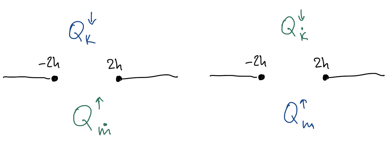
Figure 3: Two ${\bf Q}$’s from different Q-systems are glued together.

The underlying idea is to fix the apparent asymmetry between the analytic properties of ${\bf Q}$ and ${\bf P}$ (see Figure 2). Whereas ${\bf P}$ has only one branch-cut, as we argued above, ${\bf Q}$ should have a ladder of cuts going either up or down from the real axis. Following the observation in other QSCs, we notice that a section of the Riemann surface of ${\bf Q}$’s with long cut i.e. $(-\infty,-2h)\cup(2h,\infty)$ on the real axis should not have any other cuts. More specifically we require that (see Fig. 3)

$${\bf Q}_{k}^{\downarrow}(u+i0)=G_{k}^{\;\;\dot{n}}\;{\bf Q}_{\dot{n}}^{\uparrow}(u-i0)\;\;,\;\;{\bf Q}_{\dot{k}}^{\downarrow}(u+i0)=G_{\dot{k}}^{\;\;n}\;{\bf Q}_{n}^{\uparrow}(u-i0)\;\;,\;\;u\in(-2h,2h)$$ (3.25)

where $G_{k}^{\;\;\dot{n}}$ and $G_{\dot{k}}^{\;\;n}$ are two different independent constant matrices. In the studied cases of QSC they have several zero components, but in our case their exact form is still to be deduced. However, one can make a first guess by looking at the classical counterpart of the gluing relations (2.38). Using the identification (3.6) we see that it suggests $G_{1}^{\;\dot{2}}$ and $G_{2}^{\;\dot{1}}$ to be the only non-zero elements of $G_{k}^{\;\;\dot{n}}$.

For the Hodge-dual Q-functions, the gluing conditions take a similar form

$${\bf Q}^{k\downarrow}(u+i0)=G^{k}_{\;\;\dot{n}}\;{\bf Q}^{\dot{n}\uparrow}(u-i0)\;\;,\;\;{\bf Q}^{\dot{k}\downarrow}(u+i0)=G^{\dot{k}}_{\;\;n}\;{\bf Q}^{n\uparrow}(u-i0)\;\;,\;\;u\in(-2h,2h).$$ (3.26)

Like in the known cases, we assert that gluing is a symmetry of the Q-system

$$G^{k}_{\;\;\dot{n}}=\epsilon^{kl}\epsilon_{\dot{n}\dot{m}}G^{\;\;\dot{m}}_{l}\;\;,\;\;G^{\dot{k}}_{\;\;n}=\epsilon^{\dot{k}\dot{l}}\epsilon_{nm}G^{\;\;m}_{\dot{l}}\;\;,\;\;\det G=1\;.$$ (3.27)

In the following, we will choose a basis of Q-functions with specified large-$u$ asymptotics on the first sheet, described in (3.10). after this choice is made, we are not free to diagonalise the gluing matrix with a linear transformation. For this reason, we will keep track of it explicitly throughout. We leave for future work the discussion of the matrix structure of $G$ in this special basis, but as we argued above the classical limit suggests an off-diagonal structure for this matrix.

Properties of the $r$-function.

The $r$-function, which was defined in section 2.3 and allows to lower and raise indices, has interesting analyticity properties. From (2.57) we note that $r={\bf P}^{1}/{\bf P}_{2}$, meaning that $r$ (and $\dot{r}$) has at most one cut on the main sheet $(-2h,2h)$. At the same time $r={\bf Q}^{\downarrow}_{1}/{\bf Q}^{2\downarrow}$, meaning that it has only one long cut at the same time. In other words the analytic continuation from above $r^{\gamma}$ is analytic in the LHP.

$$({\bf Q}^{k\downarrow})(u+i0)=r(u+i0)\epsilon^{kl}{\bf Q}_{l}^{\downarrow}(u+i0)=r(u+i0)\epsilon^{kl}G_{l}^{\;\;\dot{n}}{\bf Q}_{\dot{n}}^{\uparrow}(u-i0),$$ (3.28)

at the same time the l.h.s. can be expressed as

$$G^{k}_{\;\;\dot{n}}\;{\bf Q}^{\dot{n}\uparrow}(u-i0)=G^{k}_{\;\;\dot{n}}\;\epsilon^{\dot{n}\dot{m}}\dot{r}(u-i0){\bf Q}_{\dot{m}}^{\uparrow}(u-i0)=\dot{r}(u-i0)\epsilon^{kl}G^{\;\;\dot{n}}_{l}{\bf Q}_{\dot{n}}^{\uparrow}(u-i0),$$ (3.29)

from where we deduce that $r(u+i0)=\dot{r}(u-i0)$. Similarly, we can start from the dotted version of the derivation above to get $r(u-i0)=\dot{r}(u+i0)$. From this consideration we see that $r(u)$ has a single quadratic cut, which connects it to $\dot{r}(u)$. This branch cut can be rationalised with the help of the Zhukovsky variable $x(u)=\frac{u+\sqrt{u-2h}\sqrt{u+2h}}{2h}$ so we can write $r$ explicitly in terms of its zeros/poles

$$r(u)=r_{0}\frac{\prod_{i}^{K_{3}-N_{R}}(x(u)-y_{3,i})\prod_{i}^{K_{\dot{3}}-N_{R}}(1/x(u)-y_{\dot{3},i})}{\prod_{i}^{K_{1}-N_{B}}(x(u)-y_{1,i})\prod_{i}^{K_{\dot{1}}-N_{B}}(1/x(u)-y_{\dot{1},i})}\;,$$ (3.30)

and $\dot{r}(u)$ is $r(u)$ with $x(u)$ replaced by $1/x(u)$. $r_{0}$ is a constant. In the above expression we assume $|y_{\dots}|\geq 1$. Finding such a simple expression for a combination of ${\bf P}$’s is an interesting novel feature of the $\text{AdS}_{3}$ QSC.

3.3 On analytic continuation

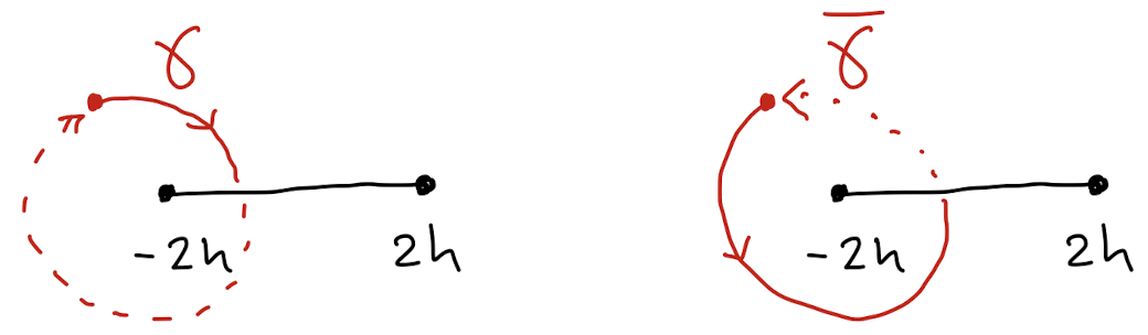
Figure 4: Two contours we use for analytic continuation

We now deduce several consequences of the discussion in the previous section. We will see that the simple set of constraints given above implies the existence of a rich mathematical structure. The Q-functions live on a Riemann surface with infinitely many sheets, but the equations we will now deduce allow us to map any one of these sheets to the first one, as is the case also for the other examples of QSCs.

As anticipated in the introduction, it will turn out that the branch cuts in this system of QSC equations cannot be quadratic. This means that, for any branch point on the Riemann surface, we can go around it in two ways, and in principle this yields two different results.

We will introduce the analytic continuation paths $\gamma$ and its inverse $\gamma^{-1}$, which we will also denote by $\bar{\gamma}$. The path $\gamma$ goes around a branch point at $2h$ in anticlockwise sense, or alternatively, it goes around the branch point at $-2h$ in clockwise sense. Since in this section we think in terms of short cuts for all the Q-functions, we can say that $\gamma$ goes through the short cut $(-2h,+2h)$ from above, while $\bar{\gamma}$ crosses it from below. The two paths are represented in figure 4. We denote the analytic continuation of any function of $u$ along these paths as $f^{\gamma}$ or $f^{\gamma^{-1}}\equiv f^{\bar{\gamma}}$. In this notation, (3.25) and (3.26) become

$$({{\bf Q}}_{k}^{\downarrow})^{\gamma}=G_{k}^{\;\;\dot{m}}{\bf Q}^{\uparrow}_{\dot{n}}\;\;,\;\;({{\bf Q}}_{\dot{k}}^{\downarrow})^{\gamma}=G_{\dot{k}}^{\;\;n}{\bf Q}_{n}^{\uparrow},\;\;\;\;({{\bf Q}}^{k\downarrow})^{\gamma}=G^{k}_{\;\;\dot{n}}\bar{{\bf Q}}^{\dot{n}\uparrow},\;\;\;\;({{\bf Q}}^{\dot{n}\downarrow})^{\gamma}=G^{\dot{a}}_{\;\;b}{\bf Q}^{b\uparrow}.$$ (3.31)

3.3.1 The ${\bf Q}\omega$-system

By defining $i$-periodic functions $\omega$:

$$\omega_{k}^{\;\;\dot{n}}=G_{k}^{\;\;\dot{m}}\Omega_{\dot{m}}^{\;\;\dot{n}}\,,\qquad\qquad\omega_{\dot{k}}^{\;\;n}=G_{\dot{k}}^{\;\;m}\Omega_{m}^{\;\;n}\,,$$ (3.32)

where $\Omega$’s are the matrices relating LHPA and UHPA bases in (3.24), (3.22), the system of equations (3.31) can be conveniently rewritten in the form

$${\bf Q}^{\downarrow\gamma}_{k}=\omega_{k}^{\;\;\dot{m}}{\bf Q}^{\downarrow}_{\dot{m}}\,,\qquad\qquad{\bf Q}_{\dot{k}}^{\downarrow\gamma}=\omega_{\dot{k}}^{\;\;m}{\bf Q}^{\downarrow}_{m}.$$ (3.33)

Notice also that by construction, it follows from the properties of the gluing matrix and $\Omega$ function that

$$\omega_{k}^{\;\;\dot{m}}\omega^{l}_{\;\;\dot{m}}=\delta_{k}^{l}\,,\qquad\qquad\text{det}(\omega)=1.$$ (3.34)

Similarly, one can introduce

$$\bar{\omega}_{\dot{n}}^{\;\;m}=G^{k}_{\;\;\dot{n}}\Omega_{\;\;k}^{m},$$ (3.35)

such that

$${\bf Q}^{\uparrow\gamma^{-1}}_{\dot{k}}=\bar{\omega}_{\dot{k}}^{\;\;m}{\bf Q}^{\uparrow}_{m}.$$ (3.36)

In what follows, we adopt a simplified notation, where ${\bf Q}^{\downarrow}$ is denoted by ${\bf Q}$ and ${\bf Q}^{\uparrow}$ is denoted by $\bar{\bf Q}$. So (3.33) and (3.36) become

$${\bf Q}_{k}^{\gamma}=\omega_{k}^{\;\;\dot{m}}{\bf Q}_{\dot{m}}\,,\qquad\qquad\bar{\bf Q}_{k}^{\bar{\gamma}}=\bar{\omega}_{k}^{\;\;\dot{m}}\bar{\bf Q}_{\dot{m}}\;.$$ (3.37)

Now let us understand the analytic continuation under the cuts of $\omega$, focusing on $\omega_{\dot{k}}^{\;\;l}$ first. Notice that the matrix $\Omega_{k}^{\;\;l}$ can be expressed as $\Omega_{k}^{\;\;l}=\bar{Q}_{a|k}^{+}Q^{a|l\;+}$ (see (C.7)) and since $Q^{a|i\;+}$ has no cut on the real axis, we only need to understand the analytic continuation of $\bar{Q}_{a|k}^{+}$. The defining relation of this function is

$$\bar{Q}_{a|k}^{+}-\bar{Q}_{a|k}^{-}={\bf P}_{a}\bar{\bf Q}_{k},$$ (3.38)

where $\bar{Q}_{a|k}^{-}$ is now analytic and invariant under the analytic continuation along $\bar{\gamma}$. Computing the discontinuity we obtain

$$\bar{Q}_{a|k}^{+\bar{\gamma}}-\bar{Q}_{a|k}^{+}={\bf P}_{a}^{\bar{\gamma}}\bar{{\bf Q}}_{k}^{\bar{\gamma}}-{\bf P}_{a}\bar{{\bf Q}}_{k}\;,$$ (3.39)

which, multiplied by $Q^{a|l\;+}$ on the left, leads to

$$(\Omega_{k}^{\;\;l})^{\bar{\gamma}}-\Omega_{k}^{\;\;l}=\bar{{\bf Q}}_{k}^{\bar{\gamma}}{\bf Q}^{l\;\bar{\gamma}}-\bar{{\bf Q}}_{k}{\bf Q}^{l}\;.$$ (3.40)

Next, multiplying these equations by $G_{\dot{k}}^{\;\;k}$, and using (3.31), we find:

$$(\omega_{\dot{k}}^{\;\;l})^{\bar{\gamma}}-\omega_{\dot{k}}^{\;\;l}={{\bf Q}}_{\dot{k}}{\bf Q}^{l\;\bar{\gamma}}-{{\bf Q}}^{\gamma}_{\dot{k}}{\bf Q}^{l}\;.$$ (3.41)

This expression generalises a similar relation found in $AdS_{5}$ and $AdS_{4}$ cases, but now we distinguish two different directions for the analytic continuation on the r.h.s.. As usual one can replace dotted to undotted indices to get a similar identity for $\omega_{k}^{\;\;\dot{l}}$.

We can use (3.41) to determine the double continuation of ${\bf Q}_{\dot{k}}$ along the contour $\gamma$ – we will then see explicitly that there may be an obstruction to the cuts being quadratic. We start by continuing (3.37) along the inverse path $\bar{\gamma}$, which gives

$${\bf Q}_{\dot{k}}=(\omega_{\dot{k}}^{\;\;l})^{\bar{\gamma}}{\bf Q}^{\bar{\gamma}}_{l}=\omega_{\dot{k}}^{\;\;l}{\bf Q}^{\bar{\gamma}}_{l}-{{\bf Q}}^{\gamma}_{\dot{k}}{\bf Q}^{l}{\bf Q}^{\bar{\gamma}}_{l}=\omega_{\dot{k}}^{\;\;l}\left(\delta_{l}^{p}-{{\bf Q}}_{l}{\bf Q}^{p}\right){\bf Q}^{\bar{\gamma}}_{p},$$ (3.42)

where the second equality is obtained by using (3.41), and recalling that ${\bf Q}_{i}{\bf Q}^{i}=0$. Inverting the factor on the r.h.s., we get

$${\bf Q}^{\bar{\gamma}}_{p}=\left(\delta_{p}^{l}+{{\bf Q}}_{p}{\bf Q}^{l}\right)\omega^{\dot{k}}_{\;\;l}{\bf Q}_{\dot{k}}\;.$$ (3.43)

From this we can compute directly the difference of the analytic continuation of the Q-function along $\gamma$ and $\bar{\gamma}$:

$${\bf Q}_{k}^{\gamma}-{\bf Q}_{k}^{\bar{\gamma}}={\bf Q}_{\dot{m}}\left(\omega_{k}^{\;\;\dot{m}}-\omega^{\dot{m}}_{\;\;\;k}\right)+{\bf Q}_{k}{\bf Q}^{l}\omega_{l}^{\;\;\dot{m}}{\bf Q}_{\dot{m}}.$$ (3.44)

In the case of $AdS_{5}$, the two terms on the r.h.s. would vanish separately, due to the symmetry properties of the analogue of $\omega$, ensuring that the branch cuts are quadratic. In our case, that does not need to be the case, since $\omega$ connects different kinds of indices and there is no reason a priori to expect any symmetry between them.

We make a further interesting observation by rewriting (3.41) in the form

$$(\omega_{\dot{k}}^{\;\;l})^{\bar{\gamma}}-{{\bf Q}}_{\dot{k}}{\bf Q}^{l\;\bar{\gamma}}=\omega_{\dot{k}}^{\;\;l}-{{\bf Q}}^{\gamma}_{\dot{k}}{\bf Q}^{l}\;\,.$$ (3.45)

This shows immediately that the combination $\omega_{\dot{k}}^{\;\;l}-{{\bf Q}}^{\gamma}_{\dot{k}}{\bf Q}^{l}\;$ is equal to its analytic continuation, and therefore the cut on the real axis disappears in this combination. We can also write it as $\omega_{\dot{k}}^{\;\;m}(\delta_{m}^{l}-{{\bf Q}}_{m}{\bf Q}^{l})$. Then taking (3.42) along $\gamma$, we get

$${\bf Q}_{\dot{k}}^{\gamma}=\omega_{\dot{k}}^{\;\;l}\left(\delta_{l}^{p}-{{\bf Q}}_{l}{\bf Q}^{p}\right){\bf Q}_{p}=\omega_{\dot{k}}^{\;\;l}{\bf Q}_{l}$$ (3.46)

with the final equality being in agreement with (3.32). The first equality allows us to find the expression for ${\bf Q}_{\dot{k}}$ continued a second time along $\gamma$:

$${\bf Q}_{\dot{k}}^{\gamma^{2}}=\omega_{\dot{k}}^{\;\;l}\left(\delta_{l}^{p}-{{\bf Q}}_{l}{\bf Q}^{p}\right){\bf Q}^{\gamma}_{p}=\omega_{\dot{k}}^{\;\;l}\left(\delta_{l}^{p}-{{\bf Q}}_{l}{\bf Q}^{p}\right)\omega_{p}^{\;\;\dot{h}}{\bf Q}_{\dot{h}}\,.$$ (3.47)

This expression confirms the potential obstruction to the cuts being quadratic. In particular, we can repeatedly iterate this continuation and obtain in general

$$({\bf Q}_{\dot{k}})^{\gamma^{n}}=U_{\dot{k}}^{\;\;p}({\bf Q}_{p})^{\gamma^{n-1}}\,,\qquad\qquad({\bf Q}_{k})^{\gamma^{n}}=\dot{U}_{k}^{\;\;\dot{p}}({\bf Q}_{\dot{p}})^{\gamma^{n-1}},$$ (3.48)

$$({\bf Q}_{\dot{k}})^{\bar{\gamma}^{n}}=\bar{U}_{\dot{k}}^{\;\;p}({\bf Q}_{p})^{\bar{\gamma}^{n-1}}\,,\qquad\qquad({\bf Q}_{k})^{\bar{\gamma}^{n}}=\dot{\bar{U}}_{k}^{\;\;\dot{p}}({\bf Q}_{\dot{p}})^{\bar{\gamma}^{n-1}},$$ (3.49)

where

$$U_{\dot{k}}^{\;\;p}\equiv\omega_{\dot{k}}^{\;\;l}\left(\delta_{l}^{p}-{{\bf Q}}_{l}{\bf Q}^{p}\right)\,,\qquad\bar{U}_{\dot{k}}^{\;\;p}\equiv\left(\dot{U}^{-1}\right)_{\dot{k}}^{\;\;p}=\left(\delta_{\dot{k}}^{\dot{m}}+{{\bf Q}}_{\dot{k}}{\bf Q}^{\dot{m}}\right)\omega^{p}_{\;\;\dot{m}},$$ (3.50)

$$\dot{U}_{k}^{\;\;\dot{p}}\equiv\omega_{k}^{\;\;\dot{m}}\left(\delta_{\dot{m}}^{\dot{p}}-{{\bf Q}}_{\dot{m}}{\bf Q}^{\dot{p}}\right),\;\;\;\dot{\bar{U}}_{k}^{\;\;\dot{p}}\equiv\left(U^{-1}\right)_{k}^{\;\;\dot{p}}=\left(\delta_{k}^{m}+{{\bf Q}}_{k}{\bf Q}^{m}\right)\omega^{\dot{p}}_{\;\;m}.$$ (3.51)

In general, following the path $\gamma^{n}$ produces a concatenation of monodromies $U\cdot\dot{U}\cdot U\cdot\dot{U}\dots$, but since there is no reason to expect $(U\cdot\dot{U})$ to be the identity matrix (or a root of the latter), this is nontrivial, meaning that each branch point has infinite order and connects to infinitely many sheets.

Notice that, while in general we expect the branch points to be non-quadratic, there are some special combinations of Q-functions that do exhibit this property. We already showed that this is the case for the ratio $r$ defined in (2.57). We now consider

$${\bf Q}^{l}{\bf Q}^{\bar{\gamma}}_{l}={\bf Q}^{l}\omega^{\dot{k}}_{\;\;l}{\bf Q}_{\dot{k}}={\bf Q}^{\dot{k}\;\gamma}{\bf Q}_{\dot{k}}\;,$$ (3.52)

where we used (3.43) and the analogous equation to (3.37) with (raised, dotted) indices. Lowering the indices with (2.57), and remembering that, as deduced above, $r^{\gamma}=r^{\bar{\gamma}}=\dot{r}$, the same relations (and their dotted version) can be written as

$$\epsilon^{kl}{\bf Q}_{k}{\bf Q}^{\bar{\gamma}}_{l}=-\epsilon^{\dot{k}\dot{l}}{\bf Q}_{\dot{k}}{\bf Q}^{\gamma}_{\dot{l}}\,,\qquad\qquad\epsilon^{kl}{\bf Q}_{k}{\bf Q}^{\gamma}_{l}=-\epsilon^{\dot{k}\dot{l}}{\bf Q}_{\dot{k}}{\bf Q}^{\bar{\gamma}}_{\dot{l}}\;.$$ (3.53)

Continuing the first equation above along $\gamma$, we get

$$\epsilon^{kl}{\bf Q}_{k}^{\gamma}{\bf Q}_{l}=-\epsilon^{\dot{k}\dot{l}}{\bf Q}_{\dot{k}}^{\gamma}{\bf Q}^{\gamma^{2}}_{\dot{l}}\;,$$ (3.54)

but due to the second equation in (3.53), the l.h.s. is also equal to $-\epsilon^{\dot{k}\dot{l}}{\bf Q}_{\dot{k}}^{\bar{\gamma}}{\bf Q}_{\dot{l}}$, meaning that the combination $\epsilon^{\dot{k}\dot{l}}{\bf Q}_{\dot{k}}^{\bar{\gamma}}{\bf Q}_{\dot{l}}=\epsilon^{kl}{\bf Q}_{k}{\bf Q}^{\gamma}_{l}$ comes back after $\gamma^{2}$!

As a final observation, we notice that, continuing the two sides of (3.45) along $\gamma$, one can also obtain an explicit equation for $\omega^{\gamma}$ in terms of quantities on the first sheet.

The main results of this section can be summarised in the following equations:

$$({\bf Q})^{\gamma}_{\dot{k}}=\omega_{\dot{k}}^{\;\;l}{\bf Q}_{l},\;\;\;\;\;\;({\bf Q}^{\dot{k}})^{\gamma}=\omega^{\dot{k}}_{\;\;l}{\bf Q}^{l},$$ (3.55)

,    and

$$\left((\omega)^{\bar{\gamma}}-\omega\right)_{\dot{k}}^{\;\;l}={\bf Q}_{\dot{k}}({\bf Q}^{l})^{\bar{\gamma}}-({\bf Q}_{\dot{k}})^{\gamma}{\bf Q}^{l},\;\;\;\;\left((\omega)^{\bar{\gamma}}-\omega\right)^{\dot{k}}_{\;\;l}=-{\bf Q}^{\dot{k}}({\bf Q}_{l})^{\bar{\gamma}}+({\bf Q}^{\dot{k}})^{\gamma}{\bf Q}_{l}.$$ (3.56)

Here, as usual, we understand that for every equation there is its double obtained by interchanging dotted and undotted indices. Together with ${\bf Q}_{i}{\bf Q}^{i}=0$, $\omega_{\dot{k}}^{\;l}\omega^{\dot{k}}_{\;m}=\delta_{m}^{l}$, and the periodicity of $\omega$, the relations (3.55),(3.56) may be taken as a self-consistent description of the QSC, which is usually dubbed ${\bf Q}\omega$-system. Bouncing back and forth between these equations, and using the fact that $\omega$ is $i$-periodic, one can obtain the result of any analytic continuation of the ${\bf Q}$-functions and $\omega$ functions, inside any cut, and express it in terms of their values on the first sheet. This is the same feature that was observed in the other examples of QSC, see the discussion in Gromov:2013pga . It is encouraging that this property is still valid here, even though the analytic structure is more complicated due to the branch points having infinite order.

3.3.2 The ${\bf P}\mu$-system

We now describe the constraints on the analytic continuation of ${\bf P}$ functions. Analogously to Gromov:2014caa , the main object in this case is the matrix $\mu$ defined as

$$\mu_{a}^{\;\;\dot{b}}\equiv Q_{a|c}^{-}\,\omega^{c}_{\;\;\dot{d}}\,Q^{\dot{b}|\dot{d}\;\;-}\,,\qquad\mu^{a}_{\;\;\dot{b}}\equiv Q^{a|c\;-}\,\omega_{c}^{\;\;\dot{d}}\,Q_{\dot{b}|\dot{d}}^{-},$$ (3.57)

which will play a role similar to $\omega$. Notice that just like in the case of $\omega$, $\mu$ has unit determinant and $\mu_{a}^{\;\;\dot{b}}\mu^{c}_{\;\;\dot{b}}=\delta_{a}^{c}$. We also notice the alternative expression

$$\mu_{a}^{\;\;\dot{b}}=\bar{Q}_{a|i}^{-}(G_{\dot{k}}^{\;\;i}\omega^{\dot{k}}_{\;\;l}G^{l}_{\;\;\dot{m}})\bar{Q}^{\dot{b}|\dot{m}\;-},$$ (3.58)

which is obtained through the relations (C.6), and will become useful in the discussion of the next section.

While $\omega$ is an $i$-periodic function on the Riemann section with short cuts, $\mu$ has a periodicity on the section with long cuts, as depicted in figure 5.

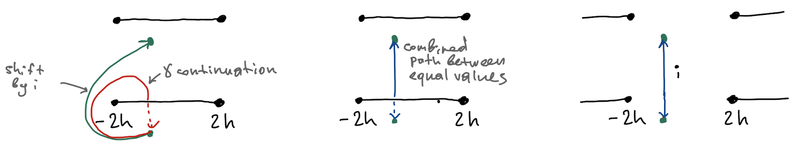
Figure 5: Periodicity of $\mu$ as a function with long cuts is identical to the property $\mu^{++}=\mu^{\gamma}$ for a section with short cuts.

Expressed in terms of a section with short cuts, this “mirror periodicity” becomes

$$\mu^{++}=(\mu)^{\gamma}.$$ (3.59)

To prove this relation (and thus also long-cut periodicity of $\mu$), we continue it along $\bar{\gamma}$ and show that the combination $(\mu^{++})^{\bar{\gamma}}-\mu$ vanishes. We can rewrite such a difference as

$$\left((\mu^{++})^{\bar{\gamma}}-\mu\right)_{a}^{\;\;\dot{b}}=Q_{a|i}^{+}\;(\omega^{i}_{\;\dot{k}})^{\bar{\gamma}}\;Q^{\dot{b}|\dot{k}\;+}-Q_{a|i}^{-}\;\omega^{i}_{\;\dot{k}}\;Q^{\dot{b}|\dot{k}\;-}.$$ (3.60)

We can now plug in $(\omega)^{\gamma^{-1}}$ from the (undotted version of) (3.56), and, in the second term, use the identities (2.53) to relate $Q_{a|i}^{-}$ and $Q_{a|i}^{+}$. We get

$$Q_{a|k}^{+}\;\left(\omega^{k}_{\;\dot{m}}+({{\bf Q}}^{k})^{\gamma}{\bf Q}_{\dot{m}}-{\bf Q}^{k}({\bf Q}_{\dot{m}})^{\bar{\gamma}}\right)Q^{\dot{b}|\dot{m}\;+}$$

$$\qquad-\,\,Q_{a|k}^{+}\left(\;\delta^{k}_{m}-{\bf Q}^{k}{\bf Q}_{m}\right)\omega^{m}_{\;\dot{m}}\left(\delta^{\dot{m}}_{\dot{k}}+{\bf Q}^{\dot{m}}{\bf Q}_{\dot{k}}\right)Q^{\dot{b}|\dot{k}\;+}=0,$$ (3.61)

where a perfect cancellation occurs due to (3.55),(3.56), establishing (3.59). We can use $\mu$ to compute the values of ${\bf P}$ on the second sheet. In particular, the definition (3.57), together with ${\bf P}_{a}=Q_{a|i}^{+}{\bf Q}^{i}$, immediately implies

$$({\bf P}_{a})^{\gamma}=\mu_{a}^{\;\dot{b}\;++}{\bf P}_{\dot{b}}=(\mu_{a}^{\;\dot{b}})^{\gamma}{\bf P}_{\dot{b}},$$ (3.62)

which is conveniently rewritten as

$$({\bf P}_{a})^{\bar{\gamma}}={\bf P}_{\dot{b}}\mu^{\dot{b}}_{\;\;a}\;.$$ (3.63)

This equation, compared to (3.37), highlights the symmetry of the construction between ${\bf P}$ and ${\bf Q}$ functions. From (3.41), it is also immediate to derive

$$(\mu_{a}^{\;\;\dot{b}})^{\gamma}-\mu_{a}^{\;\;\dot{b}}=Q_{a|k}^{+}\left(\omega^{k}_{\;\;\dot{m}}-(\omega^{k}_{\;\;\dot{m}})^{\bar{\gamma}}\right)Q^{\dot{b}|\dot{m}+}={\bf P}_{a}({\bf P}^{\dot{b}})^{\bar{\gamma}}-({\bf P}_{a})^{\gamma}{\bf P}^{\dot{b}},$$ (3.64)

which shows that the combination $\mu_{a}^{\;\;\dot{b}}+{\bf P}_{a}({\bf P}^{\dot{b}})^{\bar{\gamma}}=\left(\delta_{a}^{b}+{\bf P}_{a}{\bf P}^{b}\right)\mu_{b}^{\;\;\dot{b}}$ has no cut on the real axis. From this observation and (3.63) we also deduce

$$({\bf P}_{a})^{\gamma}=\left(\delta_{a}^{b}+{\bf P}_{a}{\bf P}^{b}\right)\mu_{b}^{\;\;\dot{b}}{\bf P}_{\dot{b}}\,,\qquad\qquad({\bf P}_{a})^{\gamma^{2}}=\left(\delta_{a}^{b}+{\bf P}_{a}{\bf P}^{b}\right)\mu_{b}^{\;\;\dot{b}}({\bf P}_{\dot{b}})^{\gamma},$$ (3.65)

and we obtain, similar to the previous discussion, that the branch points are in general connected to an infinite series of sheets, which can be reached by iterating

$$({\bf P}_{a})^{\bar{\gamma}^{n}}=\bar{W}_{a}^{\;\;\dot{b}}({\bf P}_{\dot{b}})^{\bar{\gamma}^{n-1}}\,,\qquad\qquad({\bf P}_{a})^{{\gamma}^{n}}=W^{\dot{b}}_{\;\;a}({\bf P}_{\dot{b}})^{{\gamma}^{n-1}},$$ (3.66)

with $W$, $\bar{W}$ defined by

$$W_{a}^{\;\;\dot{b}}=\left(\delta_{a}^{b}+{\bf P}_{a}{\bf P}^{b}\right)\mu_{b}^{\;\;\dot{b}}\,,\qquad\qquad\bar{W}_{a}^{\;\;\dot{b}}=\mu^{\dot{c}}_{\;\;a}\left(\delta_{\dot{c}}^{\dot{b}}-{\bf P}_{\dot{c}}{\bf P}^{\dot{b}}\right),$$ (3.67)

with $\dot{W}=(\bar{W})^{-1}$, $\dot{\bar{W}}=(W)^{-1}$ defined similarly by dotting/undotting all indices. As in the previous paragraph, we see that going around the branch point many times keeps leading to new sheets, since we expect in general that $(W\cdot\dot{W})_{a}^{\;b}\neq\delta_{a}^{b}$, being there no reason to expect otherwise.

We can summarise the finding of this section in a set of ${\bf P}\mu$ equations. For the first wing they read,

$$({\bf P}_{a})^{\bar{\gamma}}={\bf P}_{\dot{b}}\mu^{\dot{b}}_{\;\;a}\,,\qquad\qquad({\bf P}^{a})^{\bar{\gamma}}={\bf P}^{\dot{b}}\mu_{\dot{b}}^{\;\;a},$$ (3.68)

and

$$(\mu_{a}^{\;\;\dot{b}})^{\gamma}-\mu_{a}^{\;\;\dot{b}}={\bf P}_{a}({\bf P}^{\dot{b}})^{\bar{\gamma}}-({\bf P}_{a})^{\gamma}{\bf P}^{\dot{b}},\;\;\;\;(\mu^{a}_{\;\;\dot{b}})^{\gamma}-\mu^{a}_{\;\;\dot{b}}=-{\bf P}^{a}({\bf P}_{\dot{b}})^{\bar{\gamma}}+({\bf P}^{a})^{\gamma}{\bf P}_{\dot{b}}.$$ (3.69)

Together with the mirror-periodicity of $\mu$, this can also be taken as a self-consistent description of the QSC. As remarked for the ${\bf Q}\omega$-system, these equations contain enough information to map the values of ${\bf P}$ and $\mu$ functions on any sheet, back to the first main one.

4 The ABA limit

In this section, we will find an asymptotic solution for some of the Q-functions in the large-$L$ limit. This will lead us to a perfect match with the Asymptotic Bethe Ansatz for massive states, including the dressing phases.

4.1 Large-volume scaling of the QSC

To deduce the large-$L$ solution, we will use arguments developed for the $AdS_{5}$ case in Gromov:2014caa and then also successfully used for $AdS_{4}$ case to derive the ABA in Bombardelli:2017vhk . The crucial observation is that, for large $L$, some Q-functions are exponentially suppressed/enhanced, following the pattern of their large-$u$ asymptotics (3.10). Following the notation of Gromov:2014caa , we introduce a parameter $\epsilon\propto e^{-L}$ to keep track of this scaling. We then see that for large $L$ (i.e., $\epsilon\sim 0$),

$$Q_{a|i}\sim\left(\begin{array}[]{cc}1&\epsilon^{2}\\ \frac{1}{\epsilon^{2}}&1\end{array}\right),\;\;\;\;Q^{a|i}\sim\left(\begin{array}[]{cc}1&\frac{1}{\epsilon^{2}}\\ {\epsilon^{2}}&1\end{array}\right),$$ (4.5)

$${\bf Q}_{i}\sim(\epsilon^{-1},\epsilon),\;{\bf Q}^{i}\sim(\epsilon,\epsilon^{-1}),\;\;\;{\bf P}_{i}\sim(\epsilon,\epsilon^{-1}),\;{\bf P}^{i}\sim(\epsilon^{-1},\epsilon).$$ (4.6)

In the second wing, we would have exactly the same pattern for the dotted Q-functions. In addition, since the $\omega$ functions are periodic on a Riemann section with short cuts, they have constant asymptotics. We will then assume that they all scale as

$$\omega_{k}^{\;\dot{m}}\sim O(1),\;\omega^{k}_{\;m}\sim O(1),\;\omega_{\dot{k}}^{\;m}\sim O(1),\;\omega^{\dot{k}}_{\;m}\sim O(1),\;\;\;\epsilon\rightarrow 0.$$ (4.7)

We then notice that some of the QQ relations, ${\bf P}\mu$ and ${\bf Q}\omega$ equations simplify significantly. Dropping the subleading terms for $\epsilon\rightarrow 0$ we find for instance, from (3.57),

$$\mu_{1}^{\;\dot{2}}=Q_{1|k}^{-}\omega^{k}_{\;\;\dot{l}}Q^{\dot{2}|\dot{l}\;-}\sim Q_{1|1}^{-}\omega^{1}_{\;\;\dot{2}}Q^{\dot{2}|\dot{2}\;-}=Q_{1|1}^{-}\omega^{1}_{\;\;\dot{2}}Q_{\dot{1}|\dot{1}}^{-},$$ (4.8)

and similarly we get to

$$\mu^{2}_{\;\;\dot{1}}\sim Q_{1|1}^{-}\omega_{2}^{\;\;\dot{1}}Q_{\dot{1}|\dot{1}}^{-},$$ (4.9)

where we recalled that by definition $Q^{2|2}=Q_{1|1}$. Another important equation is obtained starting from ${\bf P}_{1}=(Q_{1|i}^{+}){\bf Q}^{i}$, and considering the analytic continuation along $\gamma$ (recall that $Q_{a|1}^{+}$ has no cut on the real axis). Using the ${\bf Q}\omega$-system, and then considering the large-$L$ scaling, we get

$$({{\bf P}}_{1})^{\gamma}=Q_{1|l}^{+}\omega^{l}_{\;\dot{k}}{\bf Q}^{\dot{k}}\sim Q_{1|1}^{+}\omega^{1}_{\;\dot{2}}{\bf Q}^{\dot{2}},$$ (4.10)

which will play an important role in the following derivation of the ABA.

We now proceed to deduce the form of some of the elements of the QSC in the ABA scaling. To do that, we will take as a working hypothesis the property that, for the functions $\mu_{1}^{\;\;\dot{2}}$, $\mu_{\dot{1}}^{\;\;2}$, $\mu^{\dot{1}}_{\;\;2}$, $\mu^{1}_{\;\;\dot{2}}$, the cut on the real axis becomes quadratic in the large-$L$ limit. We will see that all the solutions for massive states fall into this category.

We will also make an assumption that the gluing matrix follows the pattern one can deduce from the gluing equations in the classical limit, namely that all the diagonal elements vanish. Our derivation assumes that this is true at least in the ABA limit, but we suspect it may be true even at finite $L$ (this is what happens in $AdS_{5}$).

Finally, we will use the expressions obtained from (3.58) in the ABA limit, such as

$$\mu_{1}^{\;\;\dot{2}}\sim\bar{Q}_{1|1}^{-}(G_{\dot{k}}^{\;\;1}\omega^{\dot{k}}_{\;\;l}G^{l}_{\;\;\dot{2}})\bar{Q}_{\dot{1}|\dot{1}}^{-}\propto\bar{Q}_{1|1}^{-}\omega^{\dot{2}}_{\;\;1}\bar{Q}_{\dot{1}|\dot{1}}^{-}.$$ (4.11)

4.2 Fixing Q-functions on the first sheet

Finding $Q_{1|1}$, $\mu_{1}^{\;\;\dot{2}}$ and $\omega^{1}_{\;\;\dot{2}}$.

To determine these functions, we use the assumption on the quadratic nature of the branch point of $\mu_{1}^{\;\;\dot{2}}$ in the ABA limit. Even though this assumption could appear to be too restrictive, we will nevertheless show that in the ABA limit this extra restriction does not lead to any inconsistencies. The simplification of the analytic structure of $\mu$ is quite typical in the ABA limit – for instance in the $AdS_{5}$ case the discontinuity of $\log\mu$ appears to be a simple rational function of $x$, whereas in general it would have an infinity tower of cuts. With that in mind, we can follow closely Gromov:2014caa , and this part may be skimmed through by the reader familiar with that paper. The surprises begin from section 4.3, where the non-quadratic nature of the branch points pops up again in a crucial way.

We start by considering the function $\mu_{1}^{\;\;\dot{2}}(u+i/2)$. We take it to have a finite number of zeros on the first Riemann sheet with short cuts, and we store such zeros in a polynomial $\mathbb{Q}(u)=\prod_{i}(u-u_{i})$. We then consider

$$(F)^{2}\equiv\frac{\mu_{1}^{\;\;\dot{2}}}{\mu_{1}^{\;\;\dot{2}++}}\frac{\mathbb{Q}^{+}}{\mathbb{Q}^{-}}=\frac{\mu_{1}^{\;\;\dot{2}}}{(\mu_{1}^{\;\;\dot{2}})^{\gamma}}\frac{\mathbb{Q}^{+}}{\mathbb{Q}^{-}}$$ (4.12)

which by definition has no zeros or poles on the first Riemann sheet with short cuts. Since by our assumption the branch points of $\mu$ become quadratic in the ABA limit, using the property $(\mu)^{\gamma}=\mu^{++}\sim\mu^{\bar{\gamma}}$, it is simple to obtain the same equations as in Gromov:2014caa :

$$F(F)^{\gamma}\sim F(F)^{\bar{\gamma}}\sim\frac{\mathbb{Q}^{+}}{\mathbb{Q}^{-}}.$$ (4.13)

All the other cuts in $F$ must disappear in the ABA limit. In fact, using (4.9), and the periodicity of $\omega$, we see that $F^{2}$ can be rewritten as

$$F^{2}=\frac{Q_{1|1}^{-}\,Q_{\dot{1}|\dot{1}}^{-}}{Q_{1|1}^{+}\,Q_{\dot{1}|\dot{1}}^{+}}\frac{\mathbb{Q}^{+}}{\mathbb{Q}^{-}},$$ (4.14)

which does not have cuts in the upper half plane, while (4.11) leads us to the expression

$$F^{2}=\frac{\bar{Q}_{1|1}^{-}\,\bar{Q}_{\dot{1}|\dot{1}}^{-}}{\bar{Q}_{1|1}^{+}\,\bar{Q}_{\dot{1}|\dot{1}}^{+}}\frac{\mathbb{Q}^{+}}{\mathbb{Q}^{-}},$$ (4.15)

which shows that there are no cuts in the lower half plane either. Taking into account that $F$ has constant asymptotics at large $u$ on the first sheet, we have a simple Riemann-Hilbert problem (4.13), with the standard solution

$$F=\pm e^{i\frac{\mathcal{P}}{2}}\frac{B_{(+)}}{B_{(-)}},$$ (4.16)

with $e^{i\mathcal{P}}\equiv\prod_{i}\frac{x_{i}^{+}}{x_{i}^{-}}$, and $B_{(\pm)}(u)\equiv\sqrt{\frac{h}{x_{i}^{\mp}}}(\frac{1}{x(u)}-x_{i}^{\mp})$. The constant factor will not be very important in the current considerations.

Setting $Q_{1|1}Q_{\dot{1}|\dot{1}}\equiv\mathbb{Q}(f^{+})^{2}$, equation (4.14) then gives us a difference equation

$$\frac{f^{++}}{f}=\frac{B_{(-)}}{B_{(+)}},$$ (4.17)

where by construction $f$ should have neither poles nor zeros in the upper half plane, and power-like asymptotics. Up to a multiplicative constant, the solution is

$$f(u)\propto\text{exp}\left(\int_{-2h}^{2h}\frac{dz}{2\pi i}\log\frac{B_{(-)}(z+i0^{+})R_{(+)}(z+i0^{+})}{B_{(+)}(z+i0^{+})R_{(-)}(z+i0^{+})}\partial_{z}\log\Gamma(iz-iu)\right),$$ (4.18)

where we use $\propto$ to indicate that there could be an irrelevant constant factor in the equation. With the explicit form of $f$ in (4.18), we have fixed $Q_{1|1}Q_{\dot{1}|\dot{1}}$ completely. Noticing that $\mu_{1}^{\;\;\dot{2}}=Q_{1|1}^{-}Q_{\dot{1}|\dot{1}}^{-}\omega^{1}_{\;\;\dot{2}}\propto\bar{Q}_{1|1}^{-}\bar{Q}_{\dot{1}|\dot{1}}^{-}\omega^{1}_{\;\;\dot{2}}$, where $\omega$ should be $i$-periodic, we can also find

$$\mu_{1}^{\;\;\dot{2}}\propto\mathbb{Q}^{-}f\bar{f}^{--},\;\;\;\omega^{1}_{\;\;\dot{2}}\propto\frac{\bar{f}^{--}}{f},\;\;\;Q_{1|1}Q_{\dot{1}|\dot{1}}\propto\mathbb{Q}\,(f^{+})^{2},$$ (4.19)

where $\bar{f}$ is solution of $\bar{f}/\bar{f}^{--}=\frac{B_{(-)}}{B_{(+)}}$ with no cuts in the lower half plane and constant asymptotics. From the expression (4.14), we also see that the set of zeros of $\mathbb{Q}$ must coincide with the union of the zeros of $Q_{1|1}$ and $Q_{\dot{1}|\dot{1}}$. Therefore we split this polynomial as $\mathbb{Q}(u)\equiv\mathbb{Q}_{2}(u)\mathbb{Q}_{\dot{2}}(u)$, with $\mathbb{Q}_{2}(u)\equiv\prod_{i=1}^{K_{2}}(u-u_{2,i})$, $\mathbb{Q}_{\dot{2}}(u)\equiv\prod_{i=1}^{K_{\dot{2}}}(u-u_{\dot{2},i})$, with the understanding that $\mathbb{Q}_{2}$ contains zeros of $Q_{1|1}$, and $\mathbb{Q}_{\dot{2}}$ zeros of $Q_{\dot{1}|\dot{1}}$. This notation is chosen in anticipation of the role of the zeros in the ABA. With these conventions, we have

$$\mu_{1}^{\;\;\dot{2}}\propto\mathbb{Q}^{-}_{2}\mathbb{Q}^{-}_{\dot{2}}f_{2}f_{\dot{2}}\bar{f}^{--}_{2}\bar{f}^{--}_{\dot{2}},\;\;\;\omega^{1}_{\;\;\dot{2}}\propto\frac{\bar{f}^{--}_{2}\bar{f}^{--}_{\dot{2}}}{f_{2}\,f_{\dot{2}}},\;\;\;Q_{1|1}\propto\mathbb{Q}_{2}\,f^{+}_{2}f^{+}_{\dot{2}}\,P,\;\;\;Q_{\dot{1}|\dot{1}}\propto\mathbb{Q}_{\dot{2}}\,f^{+}_{2}f^{+}_{\dot{2}}\frac{1}{P},$$ (4.20)

with the obvious notation that $f_{\alpha}$ are solutions of $f_{\alpha}^{++}/f_{\alpha}=\frac{B_{\alpha,(-)}}{B_{\alpha,(+)}}$, with $\alpha\in\left\{2,\dot{2}\right\}$ (see appendix A), and where $P$ is a yet unfixed function of $u$ coming from splitting the product $Q_{1|1}Q_{\dot{1}|\dot{1}}$. This function should have neither zeros nor poles, and moreover $P^{-}$ cannot have any cuts in the upper half plane. On the other hand, the quantity

$$\bar{Q}_{1|1}^{+}=Q_{1|j}^{+}\Omega_{1}^{\;\;j}\sim Q_{1|1}^{+}\Omega_{1}^{\;\;1}\;\;\;\text{ for }\epsilon\rightarrow 0,$$ (4.21)

should be analytic in the lower half plane, where the matrix $\Omega$ is defined by $\omega_{\dot{a}}^{\;\;b}=G_{\dot{a}}^{\;\;c}\,\Omega_{c}^{\;\;b}$. Using the assumed classics-inspired off-diagonal property of the gluing matrix, we see that $\Omega_{1}^{\;\;1}\propto\omega_{\dot{2}}^{\;\;1}$. Then, from (4.21) and the above found solution for $\omega_{\dot{2}}^{\;\;1}$, we deduce that $\bar{Q}_{1|1}^{+}$ - which should be analytic in the lower half plane - can also be written as $\mathbb{Q}_{2}\frac{B_{2,(-)}B_{\dot{2},(-)}}{B_{2,(+)}B_{\dot{2},(+)}}\bar{f}_{2}^{--}\,\bar{f}_{\dot{2}}^{--}\,P^{+}.$ Since all the other factors already have this property, we conclude that $P^{+}$ should have no cuts in the lower half plane. All together, we found that the function $P$ cannot have any singularities or zeroes and thus is a constant (due to regularity at infinity). In conclusion, we found

$$Q_{1|1}\propto\mathbb{Q}_{2}\,f_{\dot{2}}^{+}f_{2}^{+},\;\;\;Q_{\dot{1}|\dot{1}}\propto\mathbb{Q}_{\dot{2}}\,f_{\dot{2}}^{+}f_{2}^{+},$$ (4.22)

$$\mu_{1}^{\;\;\dot{2}}\propto\mu_{\dot{1}}^{\;\;2}\propto\mathbb{Q}_{2}^{-}\,\mathbb{Q}_{\dot{2}}^{-}\;f_{2}\,\bar{f}_{2}^{--}f_{\dot{2}}\,\bar{f}_{\dot{2}}^{--},$$

$$\omega^{1}_{\;\;\dot{2}}\propto\omega^{\dot{1}}_{\;\;2}\propto\frac{\bar{f}_{2}^{--}}{f_{2}}\frac{\bar{f}_{\dot{2}}^{--}}{f_{\dot{2}}},$$

where we included the values of more $\omega$, $\mu$ functions, obtained by obvious generalisations of the argument above.

Parametrising ${\bf P}$ and ${\bf Q}$ functions.

From the $AdS_{5}$ and $AdS_{4}$ cases, we expect that a special subset of ${\bf P}$ and ${\bf Q}$ functions will converge to simple explicit expressions in the ABA limit. This is the subset of the ${\bf P}$ functions which are small, together with the ${\bf Q}$ functions that are large, for $\epsilon\rightarrow 0$. From (4.6), we see that those are ${\bf P}_{1}$, ${\bf P}^{2}$, ${\bf Q}_{1}$, ${\bf Q}^{2}$, and their dotted counterparts. We expect that their zeros on the first sheet will acquire the meaning of Bethe roots.

With this in mind, we make the following ansatz:

$${\bf P}_{1} \propto x^{-L/2}\,\mathcal{A}\times R_{\tilde{1}}B_{\tilde{\dot{1}}}\,B_{2,(-)}, {\bf P}^{2} \propto x^{-L/2}\,\mathcal{A}\times R_{\tilde{3}}B_{\tilde{\dot{3}}}B_{2,(-)},$$ (4.23)

$${\bf Q}_{1} \propto\frac{x^{L/2}}{\mathcal{A}^{\prime}}\times R_{1}B_{\dot{1}}f_{2}\frac{f_{\dot{2}}}{B_{\dot{2},(+)}}, {\bf Q}^{2} \propto\frac{x^{{L}/2}}{\mathcal{A}^{\prime}}\times R_{3}B_{\dot{3}}\,f_{2}\frac{f_{\dot{2}}}{B_{\dot{2},(+)}}\;.$$ (4.24)

Above, we have stored the zeros of the ${\bf P}$ and ${\bf Q}$ functions on the first sheet inside the Zhukovsky polynomials $R_{\alpha}$, defined in appendix A (again, the notation anticipates the role of these zeros in the ABA, but for now they are generic parameters). The other $B_{\alpha}$ and $f_{\alpha}$ factors (also defined in the appendix) are chosen for future convenience, but they do not have zeros on the first sheet. Notice that the ansatz above is fully general, because it contains the arbitrary functions of $u$ $\mathcal{A}(u)$, $\mathcal{A}^{\prime}(u)$. By construction they should have no poles or zeros on the first sheet, and moreover $\mathcal{A}$, which appears in the ${\bf P}$ functions, can have only a single cut.

Comparing with (2.57), we see that we can write the important function $r$ in two alternative ways as

$$r\propto\frac{R_{\tilde{1}}B_{\tilde{\dot{1}}}}{R_{\tilde{3}}B_{\tilde{\dot{3}}}}\propto\frac{R_{3}B_{\dot{3}}}{R_{1}B_{\dot{1}}}\;,$$ (4.25)

which means that $R_{\tilde{3}}$ and $R_{\tilde{1}}$ could have common zeroes.

Likewise we make a similar ansatz for the second wing:

$${\bf P}_{\dot{1}} \propto x^{-{L}/2}\,\dot{\mathcal{A}}\times R_{\dot{3}}^{\prime}B_{3}^{\prime}\,B_{\dot{2},(-)}, {\bf P}^{\dot{2}} \propto x^{-{L}/2}\,\dot{\mathcal{A}}\times R_{\dot{1}}^{\prime}B_{1}^{\prime}\,B_{\dot{2},(-)},$$ (4.26)

$${\bf Q}_{\dot{1}} \propto\frac{x^{{L}/2}}{\dot{\mathcal{A}}^{\prime}}\times R_{\tilde{\dot{3}}}^{\prime}B_{\tilde{3}}^{\prime}f_{\dot{2}}\,\frac{f_{2}}{B_{2,(+)}}, {\bf Q}^{\dot{2}} \propto\frac{x^{{L}/2}}{\dot{\mathcal{A}}^{\prime}}\times R_{\tilde{\dot{1}}}^{\prime}B_{\tilde{1}}^{\prime}\,f_{\dot{2}}\,\frac{f_{2}}{B_{2,(+)}}\;,$$ (4.27)

with functions $\dot{\mathcal{A}}(u)$, $\dot{\mathcal{A}}^{\prime}(u)$ having no zeroes on the main sheet. In (4.26),(4.27), we have introduced polynomials in $x$ vs $\frac{1}{x}$, $R_{\alpha}^{\prime}$ and $B_{\alpha}^{\prime}$, respectively. They are defined just like in (A.5),(A.6), but where the zeros of these polynomials (and their number) are in principle unrelated to the ones appearing in the first wing. We will however soon see that there is a simple identification. From (2.57) we again get

$$\dot{r}\propto\frac{R^{\prime}_{\dot{3}}B^{\prime}_{3}}{R^{\prime}_{\dot{1}}B^{\prime}_{1}}\propto\frac{R^{\prime}_{\tilde{\dot{1}}}B^{\prime}_{\tilde{1}}}{R^{\prime}_{\tilde{\dot{3}}}B^{\prime}_{\tilde{3}}}\;.$$ (4.28)

Furthermore, recalling that $\dot{r}^{\gamma}=r$ we get

$$\frac{R_{\tilde{1}}B_{\tilde{\dot{1}}}}{R_{\tilde{3}}B_{\tilde{\dot{3}}}}\propto\frac{R_{3}B_{\dot{3}}}{R_{1}B_{\dot{1}}}\propto\frac{B^{\prime}_{\dot{3}}R^{\prime}_{3}}{B^{\prime}_{\dot{1}}R^{\prime}_{1}}\propto\frac{B^{\prime}_{\tilde{\dot{1}}}R^{\prime}_{\tilde{1}}}{B^{\prime}_{\tilde{\dot{3}}}R^{\prime}_{\tilde{3}}}\;.$$ (4.29)

One can for example deduce that $R_{\tilde{1}}R_{1}=R_{3}R_{\tilde{3}}$ etc. from the above equation.

Fermionic duality equation.

An important constraint comes from one of the QQ relations

$$Q_{1|1}^{+}-Q_{1|1}^{-}={\bf Q}_{1}{\bf P}_{1}\;,$$ (4.30)

where we see the appearance of $Q_{1|1}$ determined in (4.22). Plugging in that value, and the ansatz (4.23),(4.24), we find, from the first equality in (4.30),

$$R_{2,(+)}B_{\dot{2},(-)}-R_{2,(-)}B_{\dot{2},(+)}\propto R_{1}\,R_{\tilde{1}}B_{\dot{1}}B_{\tilde{\dot{1}}}\frac{\mathcal{A}}{\mathcal{A}^{\prime}}\;,$$ (4.31)

where we used the property that $\mathbb{Q}_{\alpha}^{\pm}=B_{\alpha,(\pm)}R_{\alpha,(\pm)}$. Since the left hand side is a rational function in $1/x(u)$, and $\mathcal{A}$, $\mathcal{A}^{\prime}$ should have no zeros or poles on the first sheet, the ratio $\mathcal{A}(u)/\mathcal{A}^{\prime}(u)$ can only be a polynomial in the variable $\frac{1}{x(u)}$. But we can absorb any such function in a redefinition of the $B_{\tilde{\dot{1}}}$, $B_{\dot{1}}$ polynomials (which are so far completely unconstrained), so without loss of generality we can take $\mathcal{A}/\mathcal{A}^{\prime}=1$. Similar considerations arise from considering (4.30) in the second wing. From now on, therefore we take

$$\mathcal{A}(u)=\mathcal{A}^{\prime}(u)\;\;,\;\;\dot{\mathcal{A}}(u)={\dot{\mathcal{A}}}^{\prime}(u).$$ (4.32)

Notice that we still have two undetermined functions, which will be fixed in the next section. Using that ${\cal A}={\cal A}^{\prime}$, from (4.31) we obtain

$$R_{2,(+)}B_{\dot{2},(-)}-R_{2,(-)}B_{\dot{2},(+)}\propto R_{1}\,R_{\tilde{1}}B_{\dot{1}}B_{\tilde{\dot{1}}}\;.$$ (4.33)

The analogous constraint obtained by considering the second wing reads

$$B_{2,(-)}R_{\dot{2},(+)}-B_{2,(+)}R_{\dot{2},(+)}\propto B_{1}^{\prime}\,B_{\tilde{1}}^{\prime}R_{\dot{1}}^{\prime}R_{\tilde{\dot{1}}}^{\prime}\;,$$ (4.34)

and analytically continuing this equation to another sheet we find the identity

$$R_{1}\,R_{\tilde{1}}B_{\dot{1}}B_{\tilde{\dot{1}}}\propto R_{1}^{\prime}\,R_{\tilde{1}}^{\prime}B_{\dot{1}}^{\prime}B_{\tilde{\dot{1}}}^{\prime}$$ (4.35)

which implies

$$R_{1}\,R_{\tilde{1}}=R_{1}^{\prime}\,R_{\tilde{1}}^{\prime}\;.$$ (4.36)

Equations of the form (4.33) are examples of fermionic duality relations. They imply that the sets of roots with labels $1$, $2$, $3$ (or alternatively the “dual” set obtained with $1\leftrightarrow\tilde{1}$, $3\leftrightarrow\tilde{3}$) satisfy the auxiliary ABA equations of the form

$$1=\left.\frac{\mathbb{Q}^{+}_{2}B_{2,(-)}\,B_{\dot{2},(-)}}{\mathbb{Q}^{-}_{2}B_{2,(+)}\,B_{\dot{2},(+)}}\right|_{u\in\left\{\text{roots of type }1,\tilde{1},3,\tilde{3}\right\}}.$$ (4.37)

4.3 Going inside the cut: fixing the dressing phases

So far we reduced the ansatz for ${\bf P}$’s and ${\bf Q}$’s to just two unknown functions with one cut and no zeroes ${\cal A}$ and $\dot{\cal A}$ on the main sheet. In order to constrain them further, we need to go to the next sheet of their Riemann surfaces.

This will bring us to the most interesting part of the analysis, where things will be radically different than in $AdS_{5}$ and $AdS_{4}$. By studying equations of the form (4.10), which we repeat here,

$$({{\bf P}}_{1})^{\gamma}\sim Q_{1|1}^{+}\omega^{1}_{\;\dot{2}}{\bf Q}^{\dot{2}}\;\;,\;\;({{\bf P}}_{\dot{1}})^{\gamma}\sim Q_{\dot{1}|\dot{1}}^{+}\omega^{\dot{1}}_{\;2}{\bf Q}^{2}$$ (4.38)

we will find that the ${\bf P}$ and ${\bf Q}$ functions cannot have a quadratic cut even in the ABA limit. We will also be able to fix the form of the yet undetermined functions $\mathcal{A}(u)$, $\dot{\mathcal{A}}(u)$ and relate them to the dressing phases of Borsato:2013hoa .

4.3.1 The cuts cannot be quadratic

The strategy will be to compare the r.h.s. of each of the equations (4.38), with the analytic continuation of ${\bf P}$ functions, starting from their form in (4.23),(4.27). From the first equation in (4.10), in particular, we obtain:

$${\bf P}_{1}^{\gamma}=x^{L/2}({\mathcal{A}})^{\gamma}B_{\tilde{1}}R_{\tilde{\dot{1}}}\,R_{2,(-)}=\left({\mathbb{Q}}_{2}^{+}f_{\dot{2}}^{++}f_{2}^{++}\right)\left(\frac{\bar{f}_{2}\bar{f}_{\dot{2}}}{f_{2}^{++}f_{\dot{2}}^{++}}\right)\left(\frac{x^{L/2}}{\dot{\cal A}}R_{\tilde{\dot{1}}}^{\prime}B^{\prime}_{\tilde{1}}\frac{f_{2}f_{\dot{2}}}{B_{2,(+)}}\right)\;.$$ (4.39)

We noticed in the previous section that the roots of $R_{\tilde{1}}$ and $R^{\prime}_{\tilde{1}}$ satisfy the same BAE equation (4.37). The same is true for the roots of $R_{\tilde{\dot{1}}}$ and $R^{\prime}_{\tilde{\dot{1}}}$. Whereas this does not necessarily mean that all roots coincide, we will assume $R_{\tilde{1}}=R^{\prime}_{\tilde{1}}$ and $R_{\tilde{\dot{1}}}=R^{\prime}_{\tilde{\dot{1}}}$. In this case we get a nice cancellation in the above equation, which further supports this requirement. Then we get a simple relation

$$({\mathcal{A}})^{\gamma}\,\dot{\mathcal{A}}=\left(\frac{R_{2,(+)}}{R_{2,(-)}}\right)\left(\bar{f}_{2}^{--}f^{++}_{2}\bar{f}_{\dot{2}}^{--}{f}_{\dot{2}}^{++}\right)\;.$$ (4.40)

It is striking to compare this with the consequence of the second relation in (4.38), which yields

$${\mathcal{A}}\,(\dot{\mathcal{A}})^{\gamma}=\left(\frac{R_{\dot{2},(+)}}{R_{\dot{2},(-)}}\right)\,\left(\bar{f}_{2}^{--}f^{++}_{2}\bar{f}_{\dot{2}}^{--}{f}_{\dot{2}}^{++}\right).$$ (4.41)

Now we continue this relation along the reverse path $\bar{\gamma}$: the result on the l.h.s. is $(\mathcal{A})^{\bar{\gamma}}\dot{\mathcal{A}}$, and the analytic continuation of the r.h.s. is simple to compute, since the $f^{++}$, $\bar{f}^{--}$ functions have no cut on the real axis, so are left unchanged. By comparing the result with (4.40), we get the following “double-discontinuity” relations

$$\frac{\mathcal{A}^{\gamma}}{\mathcal{A}^{\bar{\gamma}}}=\frac{R_{2,(+)}}{R_{2,(-)}}\frac{B_{\dot{2},(-)}}{B_{\dot{2},(+)}}\,,\qquad\qquad\frac{\mathcal{\dot{A}}^{\gamma}}{\mathcal{\dot{A}}^{\bar{\gamma}}}=\frac{R_{\dot{2},(+)}}{R_{\dot{2},(-)}}\frac{B_{2,(-)}}{B_{2,(+)}}\;,$$ (4.42)

where the r.h.s. clearly cannot vanish (except for the vacuum) since the $R_{\alpha}$ and $B_{\alpha}$ functions have zeros on different sheets. We will now solve (4.40) and (4.41).

4.3.2 Relation to the dressing phases

In order to find the solution, without lack of generality we introduce the following ansatz in terms of $\rho$ and $\dot{\rho}$

$$\mathcal{A}=\sqrt{\frac{B_{2,(+)}}{B_{2,(-)}}}\;\sigma^{1,\text{BES}}_{2}\,\sigma^{1,\text{BES}}_{\dot{2}}\,\rho\,,\qquad\qquad\dot{\mathcal{A}}=\sqrt{\frac{B_{\dot{2},(+)}}{B_{\dot{2},(-)}}}\;\sigma^{1,\text{BES}}_{2}\,\sigma^{1,\text{BES}}_{\dot{2}}\,\dot{\rho}\;,$$ (4.43)

where, using notation from Gromov:2014caa , $\sigma^{1,{\rm BES}}_{\alpha}$ denote natural building blocks of the Beisert-Eden-Staudacher dressing factor. They satisfy

$$(\sigma^{1,{\rm BES}}_{\alpha})^{\gamma}\;\sigma^{1,{\rm BES}}_{\alpha}=(\sigma^{1,{\rm BES}}_{\alpha})^{\bar{\gamma}}\;\sigma^{1,{\rm BES}}_{\alpha}\propto f^{++}_{\alpha}\bar{f}^{--}_{\alpha}\;\;,\;\;\alpha=2,\dot{2}\;,$$ (4.44)

and are related to the product of the BES dressing factors via

$$\sigma_{\rm BES}(u)=\frac{\sigma^{1,\text{BES}}(u+\tfrac{i}{2})}{\sigma^{1,\text{BES}}(u-\tfrac{i}{2})}\;,$$ (4.45)

with the notation explained in appendix A. With this redefinition, (4.40), (4.41) become

$$(\rho)^{\gamma}\dot{\rho}\propto\sqrt{\frac{R_{2,(+)}}{R_{2,(-)}}\;\frac{B_{\dot{2},(-)}}{B_{\dot{2},(+)}}}\,,\qquad\qquad(\dot{\rho})^{\gamma}\,\rho\propto\sqrt{\frac{R_{\dot{2},(+)}}{R_{\dot{2},(-)}}\;\frac{B_{2,(-)}}{B_{2,(+)}}}\;.$$ (4.46)

In appendix B, we define the functions $\sigma^{1,{\rm extra}}$ and $\tilde{\sigma}^{1,{\rm extra}}$ which are related to the two independent dressing phases appearing in ABA equations of section 2.1 in the following way:

$$\sigma(u)=\sigma_{\rm BES}(u)\frac{\sigma^{1,{\rm extra}}(u+\tfrac{i}{2})}{\sigma^{1,{\rm extra}}(u-\tfrac{i}{2})}\,,\qquad\qquad\tilde{\sigma}(u)=\sigma_{\rm BES}(u)\frac{\tilde{\sigma}^{1,{\rm extra}}(u+\tfrac{i}{2})}{\tilde{\sigma}^{1,{\rm extra}}(u-\tfrac{i}{2})}.$$ (4.47)

In the same appendix, we also show that these extra pieces satisfy the following identities

$$({\sigma}^{1,{\rm extra}}_{\alpha})^{\gamma}\;{\tilde{\sigma}_{\alpha}}^{1,{\rm extra}}=\sqrt{\frac{R_{\alpha,(+)}}{R_{\alpha,(-)}}},\;\;\;({\tilde{\sigma}}^{1,{\rm extra}}_{\alpha})^{\gamma}\;{{\sigma}_{\alpha}}^{1,{\rm extra}}=\sqrt{\frac{B_{\alpha,(-)}}{B_{\alpha,(+)}}}\;\;,\;\;\alpha\in\left\{2,\dot{2}\right\}\;,$$ (4.48)

which we both verify directly and also independently deduce from crossing via functional arguments.

Using those building blocks, we can write

$$\rho={\sigma}_{2}^{1,{\rm extra}}{\tilde{\sigma}}_{\dot{2}}^{1,{\rm extra}}\rho_{0}\;\;,\;\;\dot{\rho}={\sigma}_{\dot{2}}^{1,{\rm extra}}{\tilde{\sigma}}_{2}^{1,{\rm extra}}\dot{\rho}_{0}\;,$$ (4.49)

where $\rho_{0}$ and $\dot{\rho}_{0}$ should be functions with square-root branch cut on the real axis satisfying

$$\rho^{\gamma}_{0}=1/\dot{\rho}_{0}\;\;,\;\;\dot{\rho}^{\gamma}_{0}=1/\rho_{0}\;.$$ (4.50)

This equation tells us that $\rho^{\gamma}_{0}$ is a function with a single cut and neither zeroes nor poles, and likewise $\dot{\rho}_{0}$ and $\rho_{0}$. In other words it can only be a power of $x$, which can be included into a re-definition of $L$. So without reducing the generality we can set $\dot{\rho}_{0}=\rho_{0}=1$. This completes the derivation of the asymptotic limit of our QSC.

4.4 Summary of results for the asymptotic limit

Let us summarise what we found for the expressions of ${\bf P}$ and ${\bf Q}$ functions. In the first wing we have:

$${\bf P}_{1} \propto x^{-L/2}\,R_{\tilde{1}}B_{\tilde{\dot{1}}}\,\sqrt{B_{2,(+)}B_{2,(-)}}\;\sigma^{1}_{2}\,\tilde{\sigma}^{1}_{\dot{2}}, {\bf P}^{2} \propto x^{-L/2}\,R_{\tilde{3}}B_{\tilde{\dot{3}}}\sqrt{B_{2,(+)}B_{2,(-)}}\;\sigma^{1}_{2}\,\tilde{\sigma}^{1}_{\dot{2}},$$ (4.51)

$${\bf Q}_{1} \propto x^{L/2}R_{1}B_{\dot{1}}\,\sqrt{\frac{B_{2,(-)}}{B_{2,(+)}}}\;\frac{f_{2}\,f_{\dot{2}}}{B_{\dot{2},(+)}\,\sigma^{1}_{2}\,\tilde{\sigma}^{1}_{\dot{2}}}, {\bf Q}^{2} \propto x^{{L}/2}R_{3}B_{\dot{3}}\,\sqrt{\frac{B_{2,(-)}}{B_{2,(+)}}}\;\frac{f_{2}\,f_{\dot{2}}}{B_{\dot{2},(+)}\,\sigma^{1}_{2}\,\tilde{\sigma}^{1}_{\dot{2}}},$$ (4.52)

and in the second wing:

$${\bf P}_{\dot{1}} \propto x^{-{L}/2}\,R_{\dot{3}}B_{3}\,\sqrt{B_{\dot{2},(+)}B_{\dot{2},(-)}}\;\;\sigma^{1}_{\dot{2}}\,\tilde{\sigma}^{1}_{2}, {\bf P}^{\dot{2}} \propto x^{-{L}/2}\,R_{\dot{1}}B_{1}\,\sqrt{B_{\dot{2},(+)}B_{\dot{2},(-)}}\;\;\sigma^{1}_{\dot{2}}\,\tilde{\sigma}^{1}_{2},$$ (4.53)

$${\bf Q}_{\dot{1}} \propto{x^{{L}/2}}\,R_{\tilde{\dot{3}}}B_{\tilde{3}}\,\sqrt{\frac{B_{\dot{2},(-)}}{B_{\dot{2},(+)}}}\,\frac{f_{2}f_{\dot{2}}}{B_{2,(+)}\,\sigma^{1}_{\dot{2}}\,\tilde{\sigma}^{1}_{2}}, {\bf Q}^{\dot{2}} \propto{x^{{L}/2}}\,R_{\tilde{\dot{1}}}B_{\tilde{1}}\,\sqrt{\frac{B_{\dot{2},(-)}}{B_{\dot{2},(+)}}}\,\frac{f_{2}f_{\dot{2}}}{B_{2,(+)}\,\sigma^{1}_{\dot{2}}\,\tilde{\sigma}^{1}_{2}}.$$ (4.54)

All relevant notations are collected in Appendix A. Having an asymptotic solution for all relevant ${\bf P}$ and ${\bf Q}$ functions we can plug them into the exact Bethe ansatz equations (2.64)-(2.69) and compare the result with the ABA (2.1).

4.5 Match with the Asymptotic Bethe Ansatz

We have finally arrived at a full specification of the Q-functions ${\bf P}_{1}$, ${\bf P}^{2}$, ${\bf Q}_{1}$, ${\bf Q}^{2}$, $Q_{1|1}$, and their dotted cousins, in the ABA limit. To obtain the Asymptotic Bethe Ansatz, we can just plug their values in the exact Bethe equations (2.64)-(2.69) following from the Q-system.

We will have the following correspondence between the zeros appearing on the first sheet of the Q-functions, and the Bethe roots appearing in the Asymptotic Bethe Ansatz: for the first wing

$$\begin{array}[]{cccc}\text{Roots:}&u_{1,k}&u_{2,k}&u_{3,k}\\ \text{Q-function:}&{\bf Q}_{1}&Q_{1|1}&{\bf Q}^{2}\end{array},\;\;\;\;\;\begin{array}[]{ccc}\text{Dual roots:}&{u}_{\tilde{1},k}&{u}_{\tilde{3},k}\\ \text{Q-function:}&{\bf P}_{1}&{\bf P}^{2}\end{array},$$ (4.55)

and for the second wing:

$$\begin{array}[]{cccc}\text{Root:}&u_{\dot{1},k}&u_{\dot{2},k}&u_{\dot{3},k}\\ \text{Q-function:}&{{\bf P}}_{\dot{1}}&{Q}_{\dot{1}|\dot{1}}&{\bf P}^{\dot{2}}\end{array},\;\;\;\;\;\begin{array}[]{ccc}\text{Dual roots:}&{u}_{\tilde{\dot{1}},k}&{u}_{\tilde{\dot{3}},k}\\ \text{Q-function:}&{\bf Q}_{\dot{1}}&{\bf Q}^{\dot{2}}\end{array}.$$ (4.56)

In particular, the exact Bethe equations (2.64)-(2.66) for the first wing reduce precisely the ABA equations (A.14)-(A.16) using the Q-functions (4.51)-(4.52). Similarly, using the exact Bethe equations of the form (2.67)-(2.69), but for the dotted Q-functions, we reproduce the ABA equations (A.17)-(A.19) using the asymptotic values (4.53)-(4.54).

As an example to demonstrate the procedure, we display the case of the middle-node equation for the first wing. At the roots of $Q_{1|1}$ i.e. at $u=u_{2,i}$ we have

$$-1=\frac{Q_{1|1}^{++}Q_{\emptyset|1}^{-}Q_{12|1}^{-}}{Q_{1|1}^{--}Q_{\emptyset|1}^{+}Q_{12|1}^{+}}=\frac{Q_{1|1}^{++}{\bf Q}_{1}^{-}{\bf Q}^{2-}}{Q_{1|1}^{--}{\bf Q}_{1}^{+}{\bf Q}^{2+}}$$

$$\qquad\qquad=\frac{(x^{-})^{L}(\sigma_{2}^{1+}\tilde{\sigma}_{\dot{2}}^{1+})^{2}{\mathbb{Q}}_{2}^{++}R_{1}^{-}B_{\dot{1}}^{-}R_{3}^{-}B_{\dot{3}}^{-}f_{2}^{[+3]}f_{\dot{2}}^{[+3]}f_{2}^{-}f_{\dot{2}}^{-}B_{2(-)}^{-}B_{2(+)}^{+}[B_{\dot{2}(+)}^{+}]^{2}}{(x^{+})^{L}(\sigma_{2}^{1-}\tilde{\sigma}_{\dot{2}}^{1-})^{2}{\mathbb{Q}}_{2}^{--}R_{1}^{+}B_{\dot{1}}^{+}R_{3}^{+}B_{\dot{3}}^{+}f_{2}^{+}\;\;\;f_{\dot{2}}^{+}\;\;\;f_{2}^{+}f_{\dot{2}}^{+}B_{2(-)}^{+}B_{2(+)}^{-}[B_{\dot{2}(+)}^{-}]^{2}},$$

where we have cancelled some terms repeated in the numerator and denominator. Next we have to use the defining property of the function $f_{\alpha}$: $\frac{f_{\alpha}^{++}}{f_{\alpha}}=\frac{B_{\alpha,(-)}}{B_{\alpha,(+)}}$ in appropriate shifted version, to re-create various $B$ functions, some of which then cancel out and some remain. At the end of this massive simplification what is left is exactly the middle-node ABA equation for the first wing, where one needs to recall how the dressing phases are reconstructed from $\sigma^{1}$ and $\tilde{\sigma}^{1}$ via $\sigma_{\alpha}=\frac{\sigma^{1+}}{\sigma^{1-}}$ and $\tilde{\sigma}_{\alpha}=\frac{\tilde{\sigma}^{1+}_{\alpha}}{\tilde{\sigma}^{1-}_{\alpha}}$:

$$-1 = \left(\frac{x^{-}}{x^{+}}\right)^{L}\times\frac{\mathbb{Q}^{++}_{2}}{\mathbb{Q}^{--}_{2}}\times\left(\sigma_{2}\right)^{2}\times\frac{R_{1}^{-}R_{3}^{-}}{R_{1}^{+}R_{3}^{+}}$$ (4.57)

$$\times\left.\frac{B_{\dot{2},(-)}^{+}\,B_{\dot{2},(+)}^{+}}{B_{\dot{2},(-)}^{-}\,B_{\dot{2},(+)}^{-}}\times\left({\tilde{\sigma}}_{\dot{2}}\right)^{2}\times\frac{B_{\dot{1}}^{-}B_{\dot{3}}^{-}}{B_{\dot{1}}^{+}B_{\dot{3}}^{+}}\right|_{u=u_{2,i}},\,\;i=1,\dots,K_{2}.$$

Finally, since the ABA equations (2.1) in the classical regime, $h\rightarrow\infty$, $L\sim K_{\alpha}\rightarrow\infty$ with fixed $\mathcal{L}\equiv L/h$ reproduce the classical limit (3.6)-(3.9) via condensation of roots into cuts in the standard way Babichenko:2014yaa , it follows that we also reproduce the classical limit from the QSC, similarly to Gromov:2014caa . Thus we see that our QSC successfully reproduces all the data from section 2.

5 Discussion and outlook

The QSCs for $AdS_{5}$ and $AdS_{4}$ have a lot in common with one another – both are based on QQ-relations dictated by the global symmetries and have similar additional analyticity constraints. We use these general features to propose a QSC for string theory on $AdS_{3}\times S^{3}\times T^{4}$ with RR charge and its $\text{CFT}_{2}$ dual. However, in contrast to the higher-dimensional QSCs, the assumption of square-root singularity near the branch points needs to be dropped. While we reproduced successfully the ABA equations for massive modes, we should still emphasise that, unlike in the previous cases Bombardelli:2017vhk ; Gromov:2014caa , we do not have the luxury of TBA equations which can be used as a starting point to derive the QSC equations. Instead, we use a bottom-up approach where we guess the QSC based on the symmetries and analogy with previous cases, and then verify it in some limits.

On the important point of the order of the cuts, we notice that if we assume them to be of the usual square-root type, unlike in previous cases, we get a further nontrivial algebraic constraint (3.47) on the Q-functions in addition to the QQ-relations, resulting in a too restrictive set of equations. So to some extent the absence of square-root behaviour is dictated by symmetries.

To be fully confident in the self-consistency and completeness of equations proposed here, we need to perform further tests beyond the matching with the ABA presented here. For example, constructing the perturbative weak coupling solution at several loop orders would be useful, which can be done with the methods of Gromov:2015vua ; Marboe:2014gma . The QSC should also reproduce the protected spectrum of the theory deBoer:1998kjm , accounting for all-order wrapping corrections not considered in the ABA analysis Baggio:2017kza ; Majumder:2021zkr . Further, it would be interesting to consider near-BPS limits where one can expect a non-trivial analytic solution at finite coupling  Gromov:2014bva ; Gromov:2014eha . Finally, one should try to solve the system numerically with high precision like in Gromov:2015wca . Another potential way to test our equations would be to re-derive the TBA equations for the massless modes Bombardelli:2018jkj ; Fontanella:2019ury .

An important question to address is whether the massless modes of the theory are already contained in our QSC proposal or whether the construction needs to be generalised in some way. For example, one might wonder whether it is possible to take a tensor product of our Q-system with an additional Q-system, perhaps based on $\mathrm{su}(2)_{\circ}$ under which the massless bosons are known to transform Borsato:2013qpa . Unfortunately, such a direct product is not compatible with the fact that massless fermions transform non-trivially under the $\mathrm{psu}(1,1|2)^{2}$ symmetry. On the other hand, the structure of the Q-system is rather rigid so it is harder to see how to augment it by an additional Q-system in a more non-trivial way.

Alternatively, it may be that incorporating the massless modes requires relaxing slightly some of the analyticity and pole-structure properties we require of the QSC. The starting point for this approach would be an attempt to derive the ABA equations including massless modes in the large-volume limit, generalising the construction we presented above. This would require new arguments, since the notion of the asymptotic regime is delicate in the presence of massless excitations, where the standard exponential large-$L$ suppression is no longer there and wrapping corrections often are of the same order as the ABA contributions. However, we point out that the QSC structure is typically very rigid and does not allow for much more freedom. In particular, given the underlying $\mathrm{psu}(1,1|2)$ algebraic structure of our system, we believe that the only place where the QQ relations could be changed would be a modification of the condition $Q_{12|12}=Q_{\dot{1}\dot{2}|\dot{1}\dot{2}}=1$. We might also have to modify the gluing condition, although this seems less natural. However, we cannot at this stage exclude the possibility that neither of these options will be necessary and the QSC presented here is already complete. To provide evidence for this claim, it would be very interesting to solve the QSC equations at finite coupling, as this would allow to perform tests in various limits, for example comparing with massless solutions at weak coupling or in the semi-classical regime Varga:2020umx .

If these additional tests can be satisfactorily performed, one can hope that $AdS_{3}$ would become an ideal background for application of SoV program for correlators Cavaglia:2018lxi . Further, combining the $AdS_{3}$ QSC spectral methods with Conformal Bootstrap Cavaglia:2021bnz techniques could provide a simpler testing ground for these ideas compared to the ${\cal N}=4$ SYM case.

Following these tests of our conjecture, it would be interesting to extend the $AdS_{3}$ QSC construction to $AdS_{3}\times S^{3}\times T^{4}$ backgrounds supported by combinations of RR and NSNS charges. The ABA for these theories is also known Lloyd:2014bsa and solutions to the crossing equations have recently been found OSS-Stef-to-appear , which should provide a further testing ground for the QSC analysis. String theory on $AdS_{3}\times S^{3}\times S^{3}\times S^{1}$ is also expected to be integrable Borsato:2015mma . Finding the QSC for this model would be particularly interesting since the global symmetry algebra is $d(2,1;\alpha)^{2}$, for which the Q-system should exhibit novel features.

It would be interesting to see whether similar techniques to the ones we have employed here can be extended to the $AdS_{2}/CFT_{1}$ integrable system Hoare:2014kma , which also features the presence of massless modes and has an algebraic structure of a similar complexity. The issue of long vs short representations, which is relevant in that case, is likely to represent an additional novelty and a reason for adapting the method even further.

6 Acknowledgments

B.S. and A.T. would like to thank Alessandro Sfondrini and Dima Volin for useful discussions during the “Integrability in Lower Dimensional AdS/CFT” workshop. A.C. and N.G. would like to thank Julius, Vladimir Kazakov and Fedor Levkovich-Maslyuk for inspiring conversations. B.S. acknowledges funding support from an STFC Consolidated Grant ‘Theoretical Particle Physics at City, University of London’ ST/T000716/1. A.T. is supported by the EPSRC-SFI grant EP/S020888/1 Solving Spins and Strings. The work of A.C. and N.G. is supported by European Research Council (ERC) under the European Union’s Horizon 2020 research and innovation programme (grant agreement No. 865075) EXACTC. N.G. is also partially supported by the STFC grant (ST/P000258/1). During the first phase of this work, A.C. was supported by the STFC grant (ST/P000258/1). We thank the Hamilton Mathematical Institute (Dublin) for hosting the workshop “Integrability in Lower Dimensional AdS/CFT”, which was a catalyst for the final stages of this work.

Appendix A Rewriting the ABA equations

Notations.

We introduce some useful notations for the ABA equations. First, using the Zhukovsky map,

$$x(u)=\frac{1}{2h}\left(u+\sqrt{u-2h}\sqrt{u+2h}\right),$$ (A.1)

we reparametrise the roots in terms of $u_{2,k}$, $u_{1,k}$, $u_{3,k}$, such that $x^{\pm}_{k}\equiv x(u_{2,k}\pm\frac{i}{2})$, $1\leq k\leq K_{{2}}$, $y_{1,k}\equiv x(u_{1,k})$, $1\leq k\leq K_{{1}}$, $y_{3,k}\equiv x(u_{3,k})$, $1\leq k\leq K_{{3}}$, and similarly for the other wing introducing $u_{\dot{2},k}$, $u_{\dot{1},k}$, $u_{\dot{3},k}$. We also accordingly rename $K_{\bar{\alpha}}\equiv K_{\dot{\alpha}}$, $\alpha=1,2,3$, as compared to the notations of section 2.1.

It is convenient to introduce the generalised Baxter polynomials

$$B_{\alpha,(\pm)}(u) \equiv \prod_{j=1}^{K_{\alpha}}\sqrt{\frac{h}{x_{\alpha,j}^{\mp}}}(\frac{1}{x(u)}-x_{\alpha,j}^{\mp}),\;\;\;\;\alpha\in\left\{2,\dot{2}\right\}$$ (A.2)

$$R_{\alpha,(\pm)}(u) \equiv \prod_{j=1}^{K_{\alpha}}\sqrt{\frac{h}{x_{\alpha,j}^{\mp}}}(x(u)-x_{\alpha,j}^{\mp}),\;\;\;\;\alpha\in\left\{2,\dot{2}\right\}$$ (A.3)

$$\mathbb{Q}_{\alpha}(u) = \prod_{j=1}^{K_{\alpha}}(u-u_{\alpha,j}),\;\;\;\;\alpha\in\left\{2,\dot{2}\right\},$$ (A.4)

$$B_{\alpha}(u) = \prod_{j=1}^{K_{\alpha}}({\frac{1}{x(u)}}-y_{\alpha,j}),\;\;\alpha\in\left\{1,3,\dot{1},\dot{3}\right\}$$ (A.5)

$$R_{\alpha}(u) = \prod_{j=1}^{K_{\alpha}}({x(u)}-y_{\alpha,j}),\;\;\alpha\in\left\{1,3,\dot{1},\dot{3}\right\}.$$ (A.6)

Notice that $B_{\alpha,(\pm)}R_{\alpha,(\pm)}\propto\mathbb{Q}_{\alpha}^{\pm}$, where the shift of a function of $u$ is defined as $g^{[\pm n]}(u)\equiv g(u+i\frac{n}{2})$, $g^{\pm}\equiv g^{[\pm 1]}$. Through the Zhukovsky map, we also consider the dressing phase a function of rapidities:

$$\sigma(u,v)\equiv\text{exp}\left(i\chi(x^{+}(u),x^{+}(v))-i\chi(x^{+}(u),x^{-}(v))+i\chi(x^{-}(u),x^{-}(v))-i\chi(x^{-}(u),x^{+}(v))\right),$$ (A.7)

and we introduce the notation:

$$\sigma_{\alpha}(u) \equiv \prod_{i=1}^{K_{\alpha}}\sigma(u,u_{\alpha,i}),\;\;\;\alpha=2,\dot{2},$$ (A.8)

and the same conventions are taken for $\tilde{\sigma}$. We also use the same notation for the BES dressing phase. We also introduce useful building blocks

$$\sigma^{1}(u,v)\equiv\text{exp}\left(i\chi(x(u),x^{+}(v))-i\chi(x(u),x^{-}(v))\right),$$ (A.9)

and similarly for $\tilde{\sigma}^{1}$, and $\sigma^{1\rm BES}$, and denote again the products over roots as

$$\sigma^{1}_{\alpha}(u)\equiv\prod_{i=1}^{K_{\alpha}}\sigma^{1}(u,u_{\alpha,i}),$$ (A.10)

with the analogous definitions made for $\tilde{\sigma}^{1}_{\alpha}(u)$ and $\sigma^{1,\text{BES}}(u)$. We then have the relation

$$\sigma_{\alpha}(u)=\frac{\sigma^{1}_{\alpha}(u+\frac{i}{2})}{\sigma^{1}_{\alpha}(u-\frac{i}{2})},$$ (A.11)

and its generalisations. It will also be useful for some of our discussions to define $\sigma^{1,\text{extra}}_{\alpha}(u)$, $\tilde{\sigma}^{1,\text{extra}}_{\alpha}(u)$ through

$$\sigma^{1}_{\alpha}(u)\equiv\sigma^{1,\text{BES}}_{\alpha}(u)\;\sigma^{1,\text{extra}}_{\alpha}(u),\;\;\;\tilde{\sigma}^{1}_{\alpha}(u)\equiv\sigma^{1,\text{BES}}_{\alpha}(u)\;\tilde{\sigma}^{1,\text{extra}}_{\alpha}(u).$$ (A.12)

Finally, for the reader’s convenience we collect the defining relations for the functions $f_{\alpha}$, $\bar{f}_{\alpha}$ appearing in the large-volume solution of the QSC:

$$\frac{f_{\alpha}^{++}}{f_{\alpha}}=\frac{B_{\alpha,(-)}}{B_{\alpha,(+)}},\;\;\;\frac{\bar{f}_{\alpha}}{\bar{f}_{\alpha}^{--}}=\frac{B_{\alpha,(-)}}{B_{\alpha,(+)}},$$ (A.13)

where $f_{\alpha}$ is assumed analytic in the upper half plane and $\bar{f}_{\alpha}$ in the lower half plane, and both are free of poles everywhere. These functions are given explicitly (up to an arbitrary multiplicative constant) by DHM-type integral representations similar to (4.18).

Compact rewriting of the ABA equations.

With the notations above, the ABA equations can be rewritten as

$$1 = \left.\frac{\mathbb{Q}^{-}_{2}\,B_{2,(+)}\,B_{\dot{2},(+)}}{\mathbb{Q}^{+}_{2}\,B_{2,(-)}\,B_{\dot{2},(-)}}\right|_{u=u_{1,i}},\,\,\,i=1,\dots,K_{1},$$ (A.14)

$$-1 = \left(\frac{x^{[-]}}{x^{[+]}}\right)^{L}\times\frac{\mathbb{Q}^{++}_{2}}{\mathbb{Q}^{--}_{2}}\times\left(\sigma_{2}\right)^{2}\times\frac{R_{1}^{-}R_{3}^{-}}{R_{1}^{+}R_{3}^{+}}$$ (A.15)

$$\times \left.\frac{B_{\dot{2},(-)}^{+}\,B_{\dot{2},(+)}^{+}}{B_{\dot{2},(-)}^{-}\,B_{\dot{2},(+)}^{-}}\times\left({\tilde{\sigma}}_{\dot{2}}\right)^{2}\times\frac{B_{\dot{1}}^{-}B_{\dot{3}}^{-}}{B_{\dot{1}}^{+}B_{\dot{3}}^{+}}\right|_{u=u_{2,i}},\,\;i=1,\dots,K_{2}$$

$$1 = \left.\frac{\mathbb{Q}^{-}_{2}\,B_{2,(+)}\,B_{\dot{2},(+)}}{\mathbb{Q}^{+}_{2}\,B_{2,(-)}\,B_{\dot{2},(-)}}\right|_{u=u_{3,i}},\,\,\,i=1,\dots,K_{3}$$ (A.16)

for the first wing, and

$$1 = \left.\frac{\mathbb{Q}^{-}_{\dot{2}}\,B_{\dot{2},(+)}\,B_{2,(+)}}{\mathbb{Q}^{+}_{\dot{2}}\,B_{\dot{2},(-)}\,B_{2,(-)}}\right|_{u=u_{\dot{1},i}},\,\,\,i=1,\dots,K_{\dot{1}},$$ (A.17)

$$-1 = \left(\frac{{x}^{[-]}}{{x}^{[+]}}\right)^{-L}\times\frac{\mathbb{Q}^{++}_{\dot{2}}}{\mathbb{Q}^{--}_{\dot{2}}}\times\left(\frac{B_{\dot{2},(-)}^{-}}{B_{\dot{2},(+)}^{+}}\right)^{2}\,\left(\sigma_{\dot{2}}\right)^{-2}\times\frac{R_{\dot{1}}^{-}R_{\dot{3}}^{-}}{R_{\dot{1}}^{+}R_{\dot{3}}^{+}}$$ (A.18)

$$\times \left.\frac{B_{2,(-)}^{-}\,B_{2,(-)}^{+}}{B_{2,(+)}^{-}\,B_{2,(+)}^{+}}\times\left(\tilde{\sigma}_{2}\right)^{-2}\times\frac{B_{1}^{-}B_{3}^{-}}{B_{1}^{+}B_{3}^{+}}\right|_{u=u_{\dot{2},i}},\,\;i=1,\dots,K_{\dot{2}}$$

$$1 = \left.\frac{\mathbb{Q}^{-}_{\dot{2}}\,B_{\dot{2},(+)}\,B_{2,(+)}}{\mathbb{Q}^{+}_{\dot{2}}\,B_{\dot{2},(-)}\,B_{2,(-)}}\right|_{u=u_{\dot{3},i}},\,\,\,i=1,\dots,K_{\dot{3}}$$ (A.19)

for the second wing.

Appendix B Functional equations for the building blocks of dressing factors

In this section, we decompose the two types of dressing factors appearing in the ABA as

$$\sigma(u,v)=\sigma_{\rm BES}(u,v)\,\sigma_{\rm extra}(u,v)\,,\qquad\tilde{\sigma}(u,v)=\sigma_{\rm BES}\,\tilde{\sigma}_{\rm extra}(u,v)\,,$$ (B.1)

and similarly

$$\sigma^{1}(u,v)=\sigma^{1,\rm BES}(u,v)\,\sigma^{1,\rm extra}(u,v)\,,\qquad\tilde{\sigma}^{1}(u,v)=\sigma^{1,\rm BES}\,\tilde{\sigma}^{1,\rm extra}(u,v),$$ (B.2)

see section A for notation. The goal of this appendix is to establish the functional relations

$${\sigma^{1,\rm extra}}(u^{\gamma},v)\;{\tilde{\sigma}^{1,\rm extra}}(u,v)=\sqrt{\frac{R_{(+)}(u,v)}{R_{(-)}(u,v)}}\,,$$ (B.3)

$${\tilde{\sigma}^{1,\rm extra}}(u^{\gamma},v)\;{{\sigma}^{1,\rm extra}}(u,v)=\sqrt{\frac{B_{(-)}(u,v)}{B_{(+)}(u,v)}}\,,$$

where in this appendix we denote

$$R_{(\pm)}(u,v)=\frac{x(u)-x^{\mp}(v)}{\sqrt{x^{\mp}(v)}},\;\;\;B_{(\pm)}(u,v)=R_{(\pm)}(u^{\gamma},v)=\frac{\frac{1}{x(u)}-x^{\mp}(v)}{\sqrt{x^{\mp}(v)}}.$$ (B.4)

These relations are important for deriving the ABA from the QSC, as they imply the crucial equation (4.48). In presenting their proof here, we will also deduce

$${\sigma^{1,\rm extra}}(u^{\gamma^{-1}},v)\;{\tilde{\sigma}^{1,\rm extra}}(u,v)=\sqrt{\frac{R_{(-)}(u,v)}{R_{(+)}(u,v)}}\,,$$ (B.5)

$${\tilde{\sigma}^{1,\rm extra}}(u^{\gamma^{-1}},v)\;{{\sigma}^{1,\rm extra}}(u,v)=\sqrt{\frac{B_{(+)}(u,v)}{B_{(-)}(u,v)}}\,.$$

B.1 Direct derivation

We start by verifying these relations directly, based on the expressions for the dressing phases of Borsato:2013hoa . From the results of this paper we deduce

$$\sigma^{1,{\rm extra}}(x,x_{2}^{\pm})=\exp i\Lambda^{LL}(x,x_{2}^{\pm}),\qquad\tilde{\sigma}^{1,{\rm extra},RL}(x,x_{2}^{\pm})=\exp i\Lambda^{RL}(x,x_{2}^{\pm}),$$ (B.6)

where we have defined

$$\Lambda^{LL}(x,x_{2}^{\pm})=-\frac{1}{2}\chi^{\rm HL}(x,x_{2}^{+})+\frac{1}{2}\chi^{\rm HL}(x,x_{2}^{-})+\frac{1}{2}\chi^{-}(x,x_{2}^{+})-\frac{1}{2}\chi^{-}(x,x_{2}^{-}),$$

$$\Lambda^{RL}(x,x_{2}^{\pm})=-\frac{1}{2}\chi^{\rm HL}(x,x_{2}^{+})+\frac{1}{2}\chi^{\rm HL}(x,x_{2}^{-})-\frac{1}{2}\chi^{-}(x,x_{2}^{+})+\frac{1}{2}\chi^{-}(x,x_{2}^{-}),$$ (B.7)

and we have the integral representations

$$\chi^{\rm HL}(x,y)=\frac{\pi}{2}\oint\frac{dw}{2\pi i}\oint\frac{dw^{\prime}}{2\pi i}\frac{\mbox{sign}(w^{\prime}+1/w^{\prime}-w-1/w)}{(x-w)(y-w^{\prime})},$$

$$\chi^{-}(x,y)=\Bigg{(}\int_{C^{+}}-\int_{C^{-}}\Bigg{)}\frac{dw}{8\pi}\frac{1}{x-w}\log\Big{[}(y-w)\Big{(}1-\frac{1}{yw}\Big{)}\Big{]}-x\leftrightarrow y,$$ (B.8)

where the full circles run counterclockwise and the contours $C^{\pm}$ denote the upper (resp., lower) half semicircle in the complex $w$-plane, running counterclockwise.

We can write

$$t(x,x_{2}^{\pm})\equiv\Big{(}\sigma^{1,{\rm extra}}\Big{)}^{2}(x,x_{2}^{\pm})=\exp\Big{[}2i\chi_{\rm extra}(x,x_{2}^{+})-2i\chi_{\rm extra}(x,x_{2}^{-})\Big{]},$$ (B.9)

and the same for the other block denoted with tilde, where

$$\chi_{\rm extra}=-\frac{1}{2}\Big{(}\chi^{\rm HL}-\chi^{-}\Big{)},\qquad\tilde{\chi}_{\rm extra}=-\frac{1}{2}\Big{(}\chi^{\rm HL}+\chi^{-}\Big{)},$$ (B.10)

and $\chi^{\rm HL}$ and $\chi^{-}$ are given by an explicit integral representation.

Equations (3.8) and (3.9) of Borsato:2013hoa are consistent with

$$\chi^{\rm HL}+({\chi}^{\rm HL})^{\gamma^{-1}}=\frac{i}{2}\log\ell^{\rm HL},\qquad\ell^{\rm HL}(x,y)=\frac{x-y}{1-{xy}},$$ (B.11)

while equations (3.14) and (3.15) in the same paper are consistent with

$$\chi^{-}-({\chi}^{-})^{\gamma^{-1}}=\frac{i}{2}\log\ell^{-},\qquad\ell^{-}(x,y)=(x-y)(1-\frac{1}{xy}).$$ (B.12)

Therefore, we can assemble

$$({\sigma}^{1,{\rm extra}})^{\gamma^{-1}}\;\tilde{\sigma}^{1,{\rm extra}}=\exp\frac{1}{4}\log\frac{\ell^{\rm HL}(x,x_{2}^{+})\ell^{-}(x,x_{2}^{+})}{\ell^{\rm HL}(x,x_{2}^{-})\ell^{-}(x,x_{2}^{-})}=\Big{(}\frac{x_{2}^{-}}{x_{2}^{+}}\Big{)}^{\frac{1}{4}}\sqrt{\frac{(x-x_{2}^{+})}{(x-x_{2}^{-})}}.$$ (B.13)

Recalling the definition of the function $R_{(\pm)}$, we can reproduce the first equation in (B.5). Likewise, we can compute

$$(\tilde{\sigma}^{1,{\rm extra}})^{\gamma^{-1}}\;\sigma^{1,{\rm extra}}=\exp\frac{1}{4}\log\frac{\ell^{\rm HL}(x,x_{2}^{+})\ell^{-}(x,x_{2}^{-})}{\ell^{\rm HL}(x,x_{2}^{-})\ell^{-}(x,x_{2}^{+})}=\Big{(}\frac{x_{2}^{+}}{x_{2}^{-}}\Big{)}^{\frac{1}{4}}\sqrt{\frac{\frac{1}{x}-x_{2}^{-}}{\frac{1}{x}-x_{2}^{+}}},$$ (B.14)

which reproduces the second equation in (B.5) if we recall the definition of the function $B_{(\pm)}$. The other relations in (B.26) also follow: since the cut is of logarithmic type, we get the reciprocal results on the r.h.s. if we cross it in the other direction.

B.2 Functional argument

Here we establish the same relations starting from the crossing equation, and assuming certain minimality requirements on its solution. The crossing equation can be decomposed into the crossing satisfied by the BES part,

$$\sigma_{\rm BES}(u_{1}^{\gamma_{\rm cross}},u_{2})\sigma_{\rm BES}(u_{1},u_{2})=\frac{x_{2}^{-}}{x_{2}^{+}}\frac{x_{1}^{-}-x_{2}^{+}}{x_{1}^{-}-x_{2}^{-}}\frac{1-\frac{1}{x_{1}^{+}x_{2}^{+}}}{1-\frac{1}{x_{1}^{+}x_{2}^{-}}},$$ (B.15)

and the crossing relations for the extra pieces:

$$\sigma_{\rm extra}(u_{1}^{\gamma_{\rm cross}},u_{2})^{2}\,\tilde{\sigma}_{\rm extra}(u_{1},u_{2})^{2} =\frac{(x_{1}^{+}-x_{2}^{+})(x_{1}^{-}-x_{2}^{-})}{(x_{1}^{-}-x_{2}^{+})(x_{1}^{+}-x_{2}^{-})},$$ (B.16)

$$\sigma_{\rm extra}(u_{1},u_{2})^{2}\,\tilde{\sigma}_{\rm extra}({u}_{1}^{\gamma_{cross}},u_{2})^{2} =\frac{\left(1-\frac{1}{x_{1}^{+}x_{2}^{-}}\right)\left(1-\frac{1}{x_{1}^{-}x_{2}^{+}}\right)}{\left(1-\frac{1}{x_{1}^{+}x_{2}^{+}}\right)\left(1-\frac{1}{x_{1}^{-}x_{2}^{-}}\right)}.$$ (B.17)

The path $\gamma_{\rm cross}$ is depicted in figure 6, and it can be decomposed as the concatenation of the path $\gamma_{-}$, entering the lower cut, followed by $\gamma_{+}$ which enters the upper cut. Notice that in our notations, different from some of the literature, both $\gamma^{\pm}$ cross one cut from below.

Figure 6: The analytic continuation path used in the crossing relation. It crosses the cuts of the dressing factors at $(-2h,2h)\pm\frac{i}{2}$, and can be decomposed into $\gamma_{+}$ and $\gamma_{-}$, which cross only one cut each.

We now follow a similar route to the one described in Vieira:2010kb , and disentangle the path $\gamma_{\rm cross}$ to derive a simpler equation for a natural building block of the solution to the crossing constraints. We will assume that, for the minimal solution, the crossing path is equivalent to the one obtained by concatenating $\gamma_{-}$ and $\gamma_{+}$ in opposite order, $\gamma_{\rm cross}\simeq\gamma_{+}\cdot\gamma_{-}\simeq\gamma_{-}\cdot\gamma_{+}$. Under this assumption, analytically continuing along the inverse path $\gamma_{+}^{-1}$ the crossing relations (B.16),(B.17), we get:

$$s(u_{1}^{\gamma_{-}},u_{2})\hat{s}(u_{1}^{\gamma_{+}^{-1}},u_{2}) = \frac{R_{(-)}^{+}B_{(+)}^{-}}{R_{(+)}^{+}B_{(-)}^{-}}\equiv A,$$ (B.18)

$$\hat{s}(u_{1}^{\gamma_{-}},u_{2})s(u_{1}^{\gamma_{+}^{-1}},u_{2}) = \frac{R_{(-)}^{-}B_{(+)}^{+}}{R_{(+)}^{-}B_{(-)}^{+}}\equiv C,$$ (B.19)

while continuing the same variable along $\gamma_{-}^{-1}$, we get:

$$s(u_{1}^{\gamma_{+}},u_{2})\hat{s}(u_{1}^{\gamma_{-}^{-1}},u_{2}) = \frac{B_{(-)}^{+}R_{(+)}^{-}}{B_{(+)}^{+}R_{(-)}^{-}}\equiv B,$$ (B.20)

$$\hat{s}(u_{1}^{\gamma_{+}},u_{2})s(u_{1}^{\gamma_{-}^{-1}},u_{2}) = \frac{B_{(-)}^{-}R_{(+)}^{+}}{B_{(+)}^{-}R_{(-)}^{+}}\equiv D,$$ (B.21)

where for simplicity of the next expressions, we denoted $s(u_{1},u_{2})\equiv\sigma_{\rm extra}(u_{1},u_{2})^{2}$, $\tilde{s}(u_{1},u_{2})\equiv\tilde{\sigma}_{\rm extra}(u_{1},u_{2})^{2}$.

From now on, we omit the second variable, since it is simply a spectator in all these functional relations, and use the notation $g^{[n]}$, described in the main text, to shift the first variable of various functions. We proceed by making the ansatz

$$s\equiv\frac{t^{+}}{t^{-}},\;\;\;\tilde{s}\equiv\frac{\tilde{t}^{+}}{\tilde{t}^{-}},$$ (B.22)

where $t$, $\tilde{t}$ are assumed to be functions with a single cut $(-2h,2h)$. The relations between these blocks and the ones introduced above is simply $t\propto(\sigma^{1,\rm extra})^{2}$, $\tilde{t}\propto(\tilde{\sigma}^{1,\rm extra})^{2}$.

Now we notice that,

$$\left(\frac{t^{+}}{t^{-}}\right)^{\gamma_{-}}=\frac{(t^{\gamma^{-1}})^{+}}{t^{-}}\,,\qquad\qquad\left(\frac{t^{+}}{t^{-}}\right)^{\gamma_{+}}=\frac{t^{+}}{(t^{\gamma^{-1}})^{-}},$$ (B.23)

and there are similar relations if we do analytic continuations along the inverse paths $\gamma_{\pm}^{-1}$, which are simply obtained by replacing $\gamma^{-1}\rightarrow\gamma$ on the r.h.s. Taking the product of (B.18),(B.20), we arrive at

$$\left(({t})^{\gamma^{-1}}\;\tilde{t}\;t\;(\tilde{t})^{\gamma}\right)^{\hat{D}-\hat{D}^{-1}}=AB=\left(\frac{R_{(-)}B_{(-)}}{R_{(+)}B_{(+)}}\right)^{\hat{D}-\hat{D}^{-1}},$$ (B.24)

where $\hat{D}\equiv\frac{i}{2}\partial_{u}$, so that in this notation $g^{n\hat{D}}\equiv g^{[n]}$. Since we look for the minimal solution to crossing, we take the simplest solution to the previous functional relation:

$$({t})^{\gamma^{-1}}\;\tilde{t}\;t\;(\tilde{t})^{\gamma}=\frac{R_{(-)}B_{(-)}}{R_{(+)}B_{(+)}}.$$ (B.25)

Similarly, considering the ratio of the same two equations, and assuming the minimal solution, we obtain

$$\left({({t})^{\gamma^{-1}}\;\tilde{t}}\right)/\left({t\;(\tilde{t})^{\gamma}}\right)=\frac{R_{(-)}B_{(+)}}{R_{(+)}B_{(-)}},$$ (B.26)

and finally from (B.25),(B.26) we read:

$$({t})^{\gamma^{-1}}\;\tilde{t}=\frac{R_{(-)}}{R_{(+)}}\,,\qquad\qquad{t}\;(\tilde{t})^{\gamma}=\frac{B_{(-)}}{B_{(+)}}.$$ (B.27)

By the same arguments from the remaining two equations we extract:

$$({t})^{\gamma}\;\tilde{t}=\frac{R_{(+)}}{R_{(-)}}\,,\qquad\qquad({t})\;(\tilde{t})^{\gamma^{-1}}=\frac{B_{(+)}}{B_{(-)}}.$$ (B.28)

Taking into account that, in the notations of the main text, $t\equiv(\sigma^{1,{\rm extra}})^{2}$, $\tilde{t}\equiv(\tilde{\sigma}^{1,{\rm extra}})^{2}$, we have therefore deduced the relations (B.3), (B.5).

Appendix C Baxter equations

Baxter equations for ${\bf Q}$ and ${\bf P}$ functions.

The obvious identities

$${\bf Q}_{k}^{++}\epsilon^{ij}{\bf Q}_{i}^{--}{\bf Q}_{j}-{\bf Q}_{k}\epsilon^{ij}{\bf Q}_{i}^{--}{\bf Q}^{++}_{j}+{\bf Q}^{--}_{k}\epsilon^{ij}{\bf Q}_{i}{\bf Q}^{++}_{j}=0\;\;,\;\;k=1,2,$$ (C.1)

can be recast as the Baxter equations

$${\bf Q}_{k}^{++}D_{1}^{-}-{\bf Q}_{k}D_{2}+{\bf Q}^{--}_{k}D_{1}^{+}=0\;\;,\;\;k=1,2,$$ (C.2)

where the coefficients can also be rewritten in terms of ${\bf P}$ functions using the QQ relations:

$$D_{1}\equiv\epsilon^{ij}{\bf Q}_{i}^{-}{\bf Q}_{j}^{+} = \epsilon_{ab}{\bf P}^{a-}{\bf P}^{b+}$$ (C.3)

$$D_{2}\equiv\epsilon^{ij}{\bf Q}_{i}^{--}{\bf Q}_{j}^{++} = \epsilon_{ab}{\bf P}^{a--}{\bf P}^{b++}-{\bf P}_{c}{\bf P}^{c--}\epsilon_{ab}{\bf P}^{a}{\bf P}^{b++}$$ (C.4)

$$= \epsilon_{ab}{\bf P}^{a--}{\bf P}^{b++}-{\bf P}_{c}{\bf P}^{c++}\epsilon_{ab}{\bf P}^{a}{\bf P}^{b--}$$

(the last equality follows from ${\bf P}_{a}{\bf P}^{a}=0$). These equations, supplemented by the large-$u$ asymptotics, give a way to compute the ${\bf Q}$ functions starting from the knowledge of the ${\bf P}$ functions.

There are also equations of the same form, obtained by replacing ${\bf P}\leftrightarrow{\bf Q}$, which may be used to compute the ${\bf P}$ functions starting from the ${\bf Q}$’s.

Finite difference relations for $Q_{a|i}$.

We close this appendix by noticing that also the middle node Q-functions can be defined as the solutions of a system of finite-difference equations, which are simply obtained from the Q-system.

One such system of relations is

$$Q_{a|i}^{+}-Q_{a|i}^{-}={\bf P}_{a}{\bf P}^{b}Q_{b|i}^{+}.$$ (C.5)

These relations can be used to construct $Q_{a|i}$ from the knowledge of the ${\bf P}$ functions. The solution is specified by requiring the appropriate asymptotic behaviour, and the region of analyticity. Solutions analytic in the upper half plane are denoted as $Q^{\downarrow}_{a|i}$. The solutions analytic in the lower half plane form an alternative basis of solutions, denoted by $Q_{a|i}^{\uparrow}$. The numerical method to compute $Q_{a|i}^{\downarrow}$ and $Q_{a|i}^{\uparrow}$ in terms of the ${\bf P}$ functions is described in Gromov:2015wca .

The two bases of solutions of the same finite-difference equations are related by an $i$-periodic matrix

$${Q}_{a|i}^{\uparrow+}=\Omega_{i}^{\;\;j}{Q}_{a|j}^{\downarrow+},\;\;\;{Q}^{a|i\uparrow+}=\Omega^{i}_{\;\;j}{Q}^{a|j\downarrow+},$$ (C.6)

which imply

$$\Omega_{k}^{\;\;l}={Q}_{a|k}^{\uparrow+}Q^{a|l\downarrow+},\;\;\;\Omega^{k}_{\;\;l}={Q}^{a|k\uparrow+}Q_{a|l\;\;}^{\downarrow+}.$$ (C.7)

Multiplying the first equation in (C.6) by ${\bf P}^{a}$ on the left, we see immediately that $\Omega$ is the same matrix relating ${\bf Q}^{\uparrow}$ and ${\bf Q}^{\downarrow}$ in (3.22). Similarly, the second equation show that

$${\bf Q}^{i\uparrow}=\Omega^{i}_{\;\;j}{\bf Q}^{j\downarrow}.$$ (C.8)

Since $Q_{a|i}$ has unit determinant and $Q_{a|i}Q^{a|j}=\delta_{i}^{j}$, from (C.7) we see immediately that $\Omega$ has unit determinant as well, and

$$\Omega^{i}_{\;\;j}\Omega_{k}^{\;\;j}=\delta^{i}_{k}.$$ (C.9)

Finally, another useful form of (C.5) is

$$Q_{a|i}^{+}-Q_{a|i}^{-}={\bf Q}_{i}{\bf Q}^{j}Q_{a|j}^{+},$$ (C.10)

which can be used to determine $Q_{a|i}$ from the knowledge of the ${\bf Q}$ functions.

References

• (1) N. Gromov, V. Kazakov, S. Leurent and D. Volin, Quantum Spectral Curve for Planar $\mathcal{N}=4$ Super-Yang-Mills Theory, Phys. Rev. Lett. 112 (2014) 011602 [1305.1939].
• (2) N. Gromov, V. Kazakov, S. Leurent and D. Volin, Quantum spectral curve for arbitrary state/operator in AdS5/CFT4, JHEP 09 (2015) 187 [1405.4857].
• (3) N. Gromov, F. Levkovich-Maslyuk, G. Sizov and S. Valatka, Quantum spectral curve at work: from small spin to strong coupling in $\mathcal{N}$ = 4 SYM, JHEP 07 (2014) 156 [1402.0871].
• (4) N. Gromov, F. Levkovich-Maslyuk and G. Sizov, Quantum Spectral Curve and the Numerical Solution of the Spectral Problem in AdS5/CFT4, JHEP 06 (2016) 036 [1504.06640].
• (5) N. Gromov and F. Levkovich-Maslyuk, Quantum Spectral Curve for a cusped Wilson line in $\mathcal{N}=4$ SYM, JHEP 04 (2016) 134 [1510.02098].
• (6) N. Gromov, F. Levkovich-Maslyuk and G. Sizov, Pomeron Eigenvalue at Three Loops in $\mathcal{N}=$ 4 Supersymmetric Yang-Mills Theory, Phys. Rev. Lett. 115 (2015) 251601 [1507.04010].
• (7) C. Marboe and D. Volin, Quantum spectral curve as a tool for a perturbative quantum field theory, Nucl. Phys. B899 (2015) 810 [1411.4758].
• (8) C. Marboe and D. Volin, The full spectrum of AdS5/CFT4 II: Weak coupling expansion via the quantum spectral curve, J. Phys. A 54 (2021) 055201 [1812.09238].
• (9) M. Alfimov, N. Gromov and V. Kazakov, QCD Pomeron from AdS/CFT Quantum Spectral Curve, JHEP 07 (2015) 164 [1408.2530].
• (10) M. Alfimov, N. Gromov and V. Kazakov, $N=4$ SYM Quantum Spectral Curve in BFKL regime, 2003.03536.
• (11) M. Alfimov, N. Gromov and G. Sizov, BFKL spectrum of $\mathcal{N}$ = 4: non-zero conformal spin, JHEP 07 (2018) 181 [1802.06908].
• (12) N. Gromov and F. Levkovich-Maslyuk, Quark-anti-quark potential in $\mathcal{N}=$ 4 SYM, JHEP 12 (2016) 122 [1601.05679].
• (13) A. Cavaglià, D. Fioravanti, N. Gromov and R. Tateo, Quantum Spectral Curve of the $\mathcal{N}=$ 6 Supersymmetric Chern-Simons Theory, Phys. Rev. Lett. 113 (2014) 021601 [1403.1859].
• (14) D. Bombardelli, A. Cavaglià, D. Fioravanti, N. Gromov and R. Tateo, The full Quantum Spectral Curve for $AdS_{4}/CFT_{3}$, JHEP 09 (2017) 140 [1701.00473].
• (15) N. Gromov and G. Sizov, Exact Slope and Interpolating Functions in N=6 Supersymmetric Chern-Simons Theory, Phys. Rev. Lett. 113 (2014) 121601 [1403.1894].
• (16) L. Anselmetti, D. Bombardelli, A. Cavaglià and R. Tateo, 12 loops and triple wrapping in ABJM theory from integrability, JHEP 10 (2015) 117 [1506.09089].
• (17) D. Bombardelli, A. Cavaglià, R. Conti and R. Tateo, Exploring the spectrum of planar AdS4/CFT3 at finite coupling, JHEP 04 (2018) 117 [1803.04748].
• (18) A. Cavaglià, N. Gromov and F. Levkovich-Maslyuk, Quantum spectral curve and structure constants in $\mathcal{N}=4$ SYM: cusps in the ladder limit, JHEP 10 (2018) 060 [1802.04237].
• (19) D. Grabner, N. Gromov and J. Julius, Excited States of One-Dimensional Defect CFTs from the Quantum Spectral Curve, JHEP 07 (2020) 042 [2001.11039].
• (20) A. Cavaglià, N. Gromov, J. Julius and M. Preti, Integrability and Conformal Bootstrap: One Dimensional Defect CFT, 2107.08510.
• (21) N. Gromov, “Introduction to the Spectrum of $N=4$ SYM and the Quantum Spectral Curve.” 2017.
• (22) A. Babichenko, B. Stefański, jr. and K. Zarembo, Integrability and the $AdS_{3}/CFT_{2}$ correspondence, JHEP 03 (2010) 058 [0912.1723].
• (23) O. Ohlsson Sax and B. Stefański, jr., Integrability, spin-chains and the $AdS_{3}/CFT_{2}$ correspondence, JHEP 08 (2011) 029 [1106.2558].
• (24) A. Cagnazzo and K. Zarembo, B-field in $AdS_{3}/CFT_{2}$ Correspondence and Integrability, JHEP 11 (2012) 133 [1209.4049].
• (25) J. R. David and B. Sahoo, Giant magnons in the D1-D5 system, JHEP 07 (2008) 033 [0804.3267].
• (26) J. R. David and B. Sahoo, S-matrix for magnons in the D1-D5 system, JHEP 10 (2010) 112 [1005.0501].
• (27) R. Borsato, O. Ohlsson Sax and A. Sfondrini, A dynamic $su(1|1)^{2}$ S-matrix for $AdS_{3}/CFT_{2}$, JHEP 04 (2013) 113 [1211.5119].
• (28) R. Borsato, O. Ohlsson Sax, A. Sfondrini, B. Stefański, jr. and A. Torrielli, The all-loop integrable spin-chain for strings on AdS${}_{3}\times S^{3}\times T^{4}$: the massive sector, JHEP 08 (2013) 043 [1303.5995].
• (29) R. Borsato, O. Ohlsson Sax, A. Sfondrini and B. Stefański, jr., Towards the All-Loop Worldsheet S Matrix for $AdS_{3}\times S^{3}\times T^{4}$, Phys. Rev. Lett. 113 (2014) 131601 [1403.4543].
• (30) R. Borsato, O. Ohlsson Sax, A. Sfondrini and B. Stefański, jr., The complete $AdS_{3}\times S^{3}\times T^{4}$ worldsheet S matrix, JHEP 10 (2014) 066 [1406.0453].
• (31) T. Lloyd, O. Ohlsson Sax, A. Sfondrini and B. Stefański, jr., The complete worldsheet S matrix of superstrings on $AdS_{3}\times S^{3}\times T^{4}$ with mixed three-form flux, Nucl. Phys. B 891 (2015) 570 [1410.0866].
• (32) R. Borsato, O. Ohlsson Sax, A. Sfondrini and B. Stefański, jr., The $AdS_{3}\times S^{3}\times S^{3}\times S^{1}$ worldsheet S matrix, J. Phys. A 48 (2015) 415401 [1506.00218].
• (33) N. Beisert, The $su(2|2)$ dynamic S-matrix, Adv. Theor. Math. Phys. 12 (2008) 945 [hep-th/0511082].
• (34) R. A. Janik, The $AdS_{5}\times S^{5}$ superstring worldsheet S-matrix and crossing symmetry, Phys. Rev. D 73 (2006) 086006 [hep-th/0603038].
• (35) C. Gomez and R. Hernandez, The Magnon kinematics of the AdS/CFT correspondence, JHEP 11 (2006) 021 [hep-th/0608029].
• (36) J. Plefka, F. Spill and A. Torrielli, On the Hopf algebra structure of the AdS/CFT S-matrix, Phys. Rev. D 74 (2006) 066008 [hep-th/0608038].
• (37) R. Borsato, O. Ohlsson Sax, A. Sfondrini, B. Stefański, jr. and A. Torrielli, Dressing phases of $AdS_{3}/CFT_{2}$, Phys. Rev. D 88 (2013) 066004 [1306.2512].
• (38) R. Borsato, O. Ohlsson Sax, A. Sfondrini and B. Stefański, jr., On the spectrum of $AdS_{3}\times S^{3}\times T^{4}$ strings with Ramond-Ramond flux, J. Phys. A 49 (2016) 41LT03 [1605.00518].
• (39) N. Beisert, B. Eden and M. Staudacher, Transcendentality and Crossing, J. Stat. Mech. 0701 (2007) P01021 [hep-th/0610251].
• (40) M. Beccaria, F. Levkovich-Maslyuk, G. Macorini and A. A. Tseytlin, Quantum corrections to spinning superstrings in $AdS_{3}\times S^{3}\times M^{4}$: determining the dressing phase, JHEP 04 (2013) 006 [1211.6090].
• (41) O. Ohlsson Sax and B. Stefański, jr., On the singularities of the RR $AdS_{3}\times S^{3}\times T^{4}$ S matrix, J. Phys. A 53 (2020) 155402 [1912.04320].
• (42) N. Dorey, D. M. Hofman and J. M. Maldacena, On the Singularities of the Magnon S-matrix, Phys. Rev. D 76 (2007) 025011 [hep-th/0703104].
• (43) A. Fontanella and A. Torrielli, Geometry of Massless Scattering in Integrable Superstring, JHEP 06 (2019) 116 [1903.10759].
• (44) A. Fontanella, O. Ohlsson Sax, B. Stefański and A. Torrielli, The effectiveness of relativistic invariance in AdS3, JHEP 07 (2019) 105 [1905.00757].
• (45) A. Cavaglià, M. Cornagliotto, M. Mattelliano and R. Tateo, A Riemann-Hilbert formulation for the finite temperature Hubbard model, JHEP 06 (2015) 015 [1501.04651].
• (46) S. Ekhammar and D. Volin, Mondromy Bootstrap for SU(2—2) Quantum Spectral Curves: From Hubbard model to AdS3/CFT2, 2109.06164.
• (47) S. Frolov and A. Sfondrini, New dressing factors for AdS3/CFT2, JHEP 04 (2022) 162 [2112.08896].
• (48) A. Cavaglià, “Quantum Spectral Curve for AdS3/CFT2: a proposal.” Talk at IGST 2022, https://indico.wigner.hu/event/1370/timetable/?view=standard.
• (49) P. Vieira and D. Volin, Review of AdS/CFT Integrability, Chapter III.3: The Dressing factor, Lett. Math. Phys. 99 (2012) 231 [1012.3992].
• (50) R. Hernandez and E. Lopez, Quantum corrections to the string Bethe ansatz, JHEP 07 (2006) 004 [hep-th/0603204].
• (51) Z. Bajnok, Review of AdS/CFT Integrability, Chapter III.6: Thermodynamic Bethe Ansatz, Lett. Math. Phys. 99 (2012) 299 [1012.3995].
• (52) M. C. Abbott and I. Aniceto, Integrable field theories with an interacting massless sector, Phys. Rev. D 103 (2021) 086017 [2002.12060].
• (53) D. Bombardelli, B. Stefański and A. Torrielli, The low-energy limit of AdS3/CFT2 and its TBA, JHEP 10 (2018) 177 [1807.07775].
• (54) M. C. Abbott and I. Aniceto, Massless Lüscher terms and the limitations of the AdS3 asymptotic Bethe ansatz, Phys. Rev. D 93 (2016) 106006 [1512.08761].
• (55) A. Dei and A. Sfondrini, Integrable S matrix, mirror TBA and spectrum for the stringy $AdS_{3}\times S^{3}\times S^{3}\times S^{1}$ WZW model, JHEP 02 (2019) 072 [1812.08195].
• (56) A. Babichenko, A. Dekel and O. Ohlsson Sax, Finite-gap equations for strings on $AdS_{3}\times S^{3}\times T^{4}$ with mixed 3-form flux, JHEP 11 (2014) 122 [1405.6087].
• (57) O. Ohlsson Sax and B. Stefański, jr., Closed strings and moduli in AdS3/CFT2, JHEP 05 (2018) 101 [1804.02023].
• (58) O. Ohlsson Sax, A. Sfondrini and B. Stefański, jr., Integrability and the Conformal Field Theory of the Higgs branch, JHEP 06 (2015) 103 [1411.3676].
• (59) A. Cavaglià, D. Fioravanti and R. Tateo, Extended Y-system for the $AdS_{5}/CFT_{4}$ correspondence, Nucl. Phys. B 843 (2011) 302 [1005.3016].
• (60) N. Gromov, V. Kazakov, S. Leurent and D. Volin, Solving the AdS/CFT Y-system, JHEP 07 (2012) 023 [1110.0562].
• (61) J. de Boer, Six-dimensional supergravity on $S^{3}\times AdS_{3}$ and 2D conformal field theory, Nucl. Phys. B 548 (1999) 139 [hep-th/9806104].
• (62) J. de Boer, Large N elliptic genus and AdS / CFT correspondence, JHEP 05 (1999) 017 [hep-th/9812240].
• (63) M. Baggio, J. de Boer and K. Papadodimas, A non-renormalization theorem for chiral primary 3-point functions, JHEP 07 (2012) 137 [1203.1036].
• (64) M. Baggio, O. Ohlsson Sax, A. Sfondrini, B. Stefański and A. Torrielli, Protected string spectrum in AdS3/CFT2 from worldsheet integrability, JHEP 04 (2017) 091 [1701.03501].
• (65) S. Majumder, O. Ohlsson, B. Stefański and A. Torrielli, Protected states in $\mbox{AdS}_{3}$ backgrounds from integrability, 2103.16972.
• (66) A. Varga, Semiclassical quantization of the mixed-flux AdS3 giant magnon, JHEP 09 (2020) 107 [2006.12080].
• (67) O. Ohlsson Sax and B. Stefański, jr., to appear, .
• (68) B. Hoare, A. Pittelli and A. Torrielli, Integrable S-matrices, massive and massless modes and the $AdS_{2}\times S^{2}$ superstring, JHEP 11 (2014) 051 [1407.0303].