LEA-Net: Layer-wise External Attention Network
for Efficient Color Anomaly Detection

Abstract

The utilization of prior knowledge about anomalies is an essential issue for anomaly detections. Recently, the visual attention mechanism has become a promising way to improve the performance of CNNs for some computer vision tasks. In this paper, we propose a novel model called Layer-wise External Attention Network (LEA-Net) for efficient image anomaly detection. The core idea relies on the integration of unsupervised and supervised anomaly detectors via the visual attention mechanism. Our strategy is as follows: (i) Prior knowledge about anomalies is represented as the anomaly map generated by unsupervised learning of normal instances, (ii) The anomaly map is translated to an attention map by the external network, (iii) The attention map is then incorporated into intermediate layers of the anomaly detection network. Notably, this layer-wise external attention can be applied to any CNN model in an end-to-end training manner. For a pilot study, we validate LEA-Net on color anomaly detection tasks. Through extensive experiments on PlantVillage, MVTec AD, and Cloud datasets, we demonstrate that the proposed layer-wise visual attention mechanism consistently boosts anomaly detection performances of an existing CNN model, even on imbalanced datasets. Moreover, we show that our attention mechanism successfully boosts the performance of several CNN models.

1. Introduction

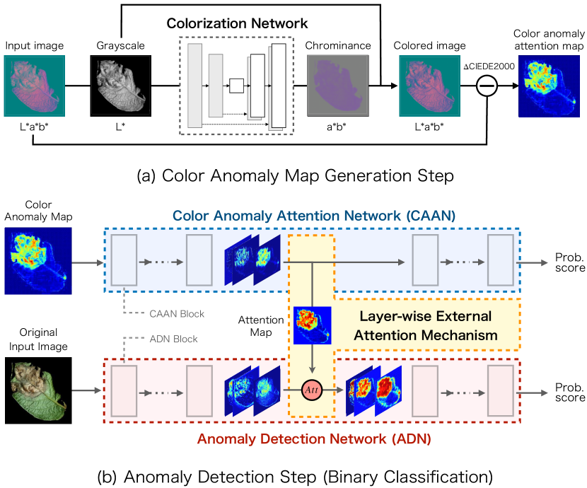
Figure 1: Overview of the color anomaly detection.

Anomaly detection is a technique to identify irregular or unusual patterns in datasets. Especially, anomaly detection for imaging data is a powerful and core technology for various kinds of real-world problems including medical diagnosis (Rezvantalab, Safigholi, and Karimijeshni 2018; Cao et al. 2018), plant healthcare (Ferentinos 2018), production quality controls, and disaster detection (Minhas and Zelek 2019; Natarajan, Mao, and Chia 2019). Over the last decade, many researchers have shown great interest in establishment of automatic anomaly detection techniques for a huge image dataset driven by breakthroughs in deep learning. Based on types of machine learning, these anomaly detection techniques can be roughly classified into three categories: supervised, semi-supervised, and unsupervised approaches. Although there are advantages and disadvantages with each approach, the fundamental challenge that should be overcome is on how we detect anomalies efficiently based on limited numbers of anomalous instances.

Convolutional neural network (CNN) is a commonly used artificial network for various computer vision tasks including image recognition and image segmentation. Using a huge dataset of labeled images, CNNs have realized a state-of-the-art image anomaly detection in a real-world applications (Hughes and Salathe 2016; Minhas and Zelek 2019). However, anomaly detectors based on CNN suffer from a lack of labeled images and low anomaly instances. Some studies have proposed ideas for overcoming this point by improving learning efficiency of CNN. In particular, one introduced active learning (Goernitz et al. 2013) and the other employed transfer learning (Minhas and Zelek 2019) for that purpose.

Approaches based on unsupervised learning are the most popular way for anomaly detection, because they do not require labeled anomalous instances to train anomaly detectors. The simple strategy of unsupervised image anomaly detections relies on a training of reconstruction processes for normal images using a deep convolutional autoencoder (Haselmann, Gruber, and Tabatabai 2018). However, the autoencoder sometimes fails to reconstruct fine structures. Consequently, it outputs immoderate blurry structures. Recently, generative adversarial networks (GAN) have been used for image anomaly detection to overcome this point. AnoGAN (Schlegl et al. 2017) firstly employed GAN to image anomaly detection. In applications of medical image processing, AnoGAN and its extensions (Zenati et al. 2018; Akcay, Atapour-Abarghouei, and Breckon 2018) realized to detect minute anomalies. More recently, the idea of AnoGAN was extended in terms of color reconstructability to realize sensitive detection of color anomalies (Katafuchi and Tokunaga 2021). It is a common procedure in unsupervised anomaly detection to define the difference between the original image and the reconstructed image as Anomaly Score.

Although unsupervised anomaly detectors can eliminate the labeling cost of anomalous instances for a training step, there are some drawbacks. First, they tend to overlook small and minute anomalies because Anomaly Score is defined based on the distance of the normal images and test images. In other words, the detection performance strongly depends on whether we can design a good Anomaly Score for each purpose. Also, we should tune carefully the appropriate threshold of Anomaly Score for successful classifications of normal and anomalous instances. In most practices, this process requires painful trial and error.

Nowadays, the technique called visual attention mechanism is attracting much attention in computer vision (Zhao, Jia, and Koltun 2020). Attention Branch Network (ABN) is a CNN with a branching structure called Attention Branch (Fukui et al. 2019). Attention map that output from Attention Branch represent visual explanations, which enables humans to understand the decision-making process of CNN. Further, the authors reported that the attention map contributes to improving the performances of CNN for several image classification tasks. Since then, researchers in computer vision have attempted to build the technique that finely induces the attention of CNN to informative regions in images. For the last several years, it has been shown that such technique is promising for improving the performance of CNN for several computer vision tasks involving image classification and segmentation (Fukui et al. 2019; Emami et al. 2020). Inspired by these studies, one may think to introduce the visual attention mechanism to image anomaly detection. However, visual attention modules including ABN basically relies on self-attention mechanisms (Hu et al. 2020; Woo et al. 2018). Accordingly, the attention quality of the modules strongly depends on the performance of the network itself, which means that existing visual attention mechanisms would not be able to boost the performance of anomaly detectors directly.

In this paper, we propose Layer-wise External Attention Network (LEA-Net) to boost CNN-based anomaly detectors. As we mentioned above, purely unsupervised anomaly detectors do not utilize anomalous instances at all for training. As a result, they tend to overlook small and minute anomalies, or conversely, incur high false positives. On the other hand, purely supervised approaches suffer from lack of labeled images, especially from lack of anomalous instances. We tackle these problems by integrating supervised and unsupervised anomaly detectors via visual attention mechanism. Recent progress in visual attention mechanism strongly implies that there must be a way to utilize prior knowledge for anomaly detection. Our expectation is that the anomaly map that generated from an unsupervised anomaly detector is powerless by itself for efficient anomaly detection but useful to boost supervised anomaly detectors. Moreover, we expect that such a boosting approach contributes to reduce developing cost of anomaly detectors because we can divert existing image classifiers for image anomaly detection.

Our overall strategy is as follows: (i) Prior knowledge on anomalies is represented as the anomaly map, which is generated through unsupervised learning of normal instances, (ii) The anomaly map is translated to an attention map by the external network, (iii) The attention map is then incorporated into intermediate layers of the anomaly detection network. We note that this layer-wise external attention can be applied to any CNN model with an end-to-end training manner. For a pilot study, we focus on color anomaly detection tasks because color anomalies are comparatively easy to represent based on CIEDE2000 color difference (Katafuchi and Tokunaga 2021). We examined the effectiveness of LEA-Net through extensive experiments using real-world publicly available datasets including PlantVillage, MVTec AD, and Cloud datasets. The results demonstrated that the proposed layer-wise visual attention mechanisms consistently boost performances of anomaly detectors even on imbalanced datasets. Moreover, it was shown that the attention mechanism works well for multiple feed-forward CNN models.

Our contributions are as follows:

• We propose a novel anomaly detection model called Layer-wise External Attention Networks (LEA-Net) for efficient image anomaly detection with a limited number of anomalous instances.

• We showed that our layer-wise external attention mechanism successfully boosts the performance of the color image anomaly detectors, even for small and imbalanced training datasets.

• We found that the layer-wise external attention mechanism is effective for existing feed-forward CNN models.

• We provide our code and models as open source at https://github.com/RxstydnR/LEA-Net.

2. Related Work

The proposed approach is an integration of unsupervised image translation and supervised anomaly detection. Most recently, a simpler approach was adopted in a task of automatic identification for thyroid nodule lesions in X-ray computed tomography images (Li et al. 2021). The technique uses binary segmentation results obtained from U-Net as inputs for supervised image classifiers. The authors showed that the binary segmentation as a preprocessing for an image classification contributes to improving anomaly detection in a real-world problem. Looking for a somewhat similar setting, Convolutional Adversarial Variational autoencoder with Guided Attention (CAVGA) uses an anomaly map in a weakly supervised setting to localize anomalous regions (Venkataramanan et al. 2020). Through experiments for image anomaly detection using MVTec AD, CAVGA achieved SOTA results. These two studies imply that the introduction of a visual attention map has a great potential for image anomaly detection.

A visual attention mechanism typically refers to the process of refinement or enhancement of image features for recognition tasks. The human perceptual system tends to preferentially capture information relevant to the current task, rather than processing all information (Reynolds and Chelazzi 2004; Chun, Golomb, and Turk-Browne 2011). Visual attention mechanisms basically imitate this for image classification (Hu et al. 2020; Wang et al. 2017; Woo et al. 2018; Lee, Kim, and Nam 2019; Wang et al. 2020; Yang et al. 2021). Most image classifiers with visual attention adopt a self-attention module that works in plug-and-play to existing models. In such specifications, the effectiveness of visual attention strongly depends on the performance of the main body of the model: this is a limitation of self-attention approaches. Attention Branch Network (ABN) (Fukui et al. 2019) overcame this problem by interactive edit of attention map. It enabled us to induce focus points of CNN to more informative regions on images through the correction of attention map. Another similar visual attention mechanism is Attention Transfer based on knowledge distillation (Zagoruyko and Komodakis 2017). In knowledge distillation, a smaller network called student network receives prior knowledge from a larger network called teacher network (Hinton, Vinyals, and Dean 2015). The idea of Attention Transfer relies on an assumption that a teacher network tends to focus on a more informative area than does a student network.

We designed LEA-Net inspired by ABN and Attention Transfer Network with several points of improvement. Our method does not require any user-interaction to control focus points of CNN. The training of LEA-Net goes on fully automatically through a collaboration of two networks that we call external network and anomaly detection network. The external network adjusts the strength of attention with progress of training to avoid excessive effects of visual attention mechanism in the early stage of training. Also, we note that the effectiveness of the layer-wise external attention mechanism is not constrained by the teacher network unlike Attention Transfer Network.

3. Proposed Method

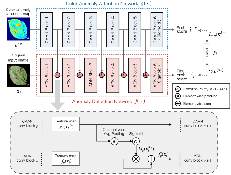
Figure 2: Overall structure of LEA-Net.

As we mentioned in Section 1, we focus on color anomaly detection tasks for a pilot study. In Fig.1, we illustrate the overview of our color anomaly detection. The procedure can be divided into two steps: (a) color anomaly map generation and (b) color anomaly detection. Details will be described below.

3-1. Color Anomaly Map Generation

In step (a), a grayscale image is firstly obtained from the input color image represented in $L^{*}a^{*}b^{*}$ color space. Then, the grayscale image is reconverted to a color image using U-Net (Ronneberger, Fischer, and Brox 2015). To supplement, the color information $a^{*}b^{*}$(chrominance) is predicted based on $L^{*}$ (luminance) information in the $L^{*}a^{*}b^{*}$ color space. Second, the predicted $a^{*}b^{*}$ is combined with the $L^{*}$ of input to produce the resulting colored image in $L^{*}a^{*}b^{*}$ color space. The U-Net learns in advance the process of color reconstruction with normal instances only. Then, a color anomaly map is generated by calculating CIEDE2000 (Sharma, Wu, and Dalal 2005) color difference between the reconstructed image and the original image. For details of the color anomaly generation, see (Katafuchi and Tokunaga 2021).

Here we consider data augmentation because the concern of this study is on anomaly detection with comparatively few training data. Empirically, the color reconstruction often fails for quite bright or dark images. Hence, we use Fancy PCA image augmentation (Krizhevsky, Sutskever, and Hinton 2012) to amplify the variation of image luminances.

3-2. Color Anomaly Attention Network (CAAN)

We describe the detail of Fig. 1(b): Anomaly detection step. In this step, we use two different image classifiers. One is Color Anomaly Attention Network (CAAN), which converts the anomaly map to an attention map. Except for color anomaly detection, we call the network External Network. The other is Anomaly Detection Network (ADN), which outputs the final decision for anomaly detection.

It is desirable that CAAN is a lightweight and effective model to work in plug-and-play without a massive increase in parameters. To that purpose, architectures of CAAN were designed based on MobileNet and ResNet. Detailed structures of CAAN are described in Table 1. The structure of MobileNet-based CAAN is exactly same as MobileNetV3-Small (Howard et al. 2019). Besides, the structure of ResNet-based CAAN is configured by simply stacking five residual blocks (He et al. 2016). We note that these two models are generic for image classifiers. Therefore, they can be replaced easily by other networks.

3-3. Anomaly Detection Network (ADN)

The role of ADN is to make the final decision for image anomaly detection utilizing prior knowledge received from CAAN. We adopted ResNet18 and VGG16 for ADN, both of which are well-known and widely-used CNN for image classifications. The number of downsampling points in ADN should be the same or larger than that of CAAN due to the reasons described below.

Table 1: Structures of CAAN: MobileNet-based network and ResNet-based network. The convolution layers are denoted as $\{$conv2d, $\langle$receptive field$\rangle$x$\langle$receptive field$\rangle$, $\langle$number of channels$\rangle$$\}$. ”bneck” denotes bottleneck structure; see (Howard et al. 2019).

block name	ResNet-based CAAN	MobileNet-like CAAN
input (256$\times$256$\times$1 Anomaly map)
block 1	conv2d, 7x7, 64	conv2d, 3x3, 16
Attention Output Point 1
block 2	conv2d, 3x3, 64 conv2d, 3x3, 64	bneck, 3x3, 16
Attention Output Point 2
block 3	conv2d, 3x3, 128 conv2d, 3x3, 128	[bneck, 3x3, 24] $\times$ 2
Attention Output Point 3
block 4	conv2d, 3x3, 256 conv2d, 3x3, 256	[bneck, 5x5, 40] $\times$ 3 [bneck, 5x5, 48] $\times$ 2
Attention Output Point 4
block 5	conv2d, 3x3, 512 conv2d, 3x3, 512	[bneck, 5x5, 96]$\times$3
Attention Output Point 5
block 6	average pool 2-d fc sigmoid	conv2d, 1x1, 576 average pool conv2d, 1x1, 1280 conv2d, 1x1, 2 sigmoid
Params	4.491M	3.042M

3-4. The overall structure of LEA-Net

In Fig. 2, we illustrate the overall structure of LEA-Net. As shown in Fig. 2, CAAN has five feature extraction blocks. In other words, CAAN has five alternatives for outputting attention maps for layer-wise visual attention. Simultaneously, ADN can have attention points up to five. In this study, the attention point in ADN is limited to one to avoid the performance deterioration of ADN.

In the training process, both CAAN and ADN are optimized by passing through the gradients of the CAAN and ADN network during back propagation. Let us denote the $i$th original input image by ${\mathbf{x}}_{i}\in\mathbb{R}^{H\times W\times 3}$. Let ${\mathbf{x}}^{Att}_{i}\in\mathbb{R}^{H\times W}$ be the $i$th color anomaly map. Also, let $y_{i}\in\left\{0,1\right\}$ be a corresponding ground-truth label. Further, let $L_{Att}$ and $L_{AD}$ be loss functions for CAAN and for ADN, respectively. The loss function for the entire classification network can be expressed as a sum of the two loss functions as:

$$L = L_{Att}+L_{AD}$$ (1)

$$= BCE(g({\mathbf{x}_{i}^{Att}}),y_{i})+BCE(f({\mathbf{x}_{i}}),y_{i}).$$

Here, $g(\cdot)$ and $f(\cdot)$ denote the output of CAAN and that of ADN, respectively. Also, $BCE(\cdot)$ denotes the binary crossentropy. We designed the loss function expecting that CAAN modifies attention maps more effectively during training likewise ABN.

3-5. Attention Mechanism

Let us denote the $p$-th attention point in ADN by
$A_{p}~{}(p\in\{1,2,3,4,5\})$. Also, let $M_{p}~{}\in~{}\mathbb{R}^{H_{p}\times W_{p}}$ be the attention map at $A_{p}$. The concept of layer-wise external attention is illustrated in the lower half of Fig. 2. Let $g_{p}(\mathbf{x}^{Att}_{i})\in\mathbb{R}^{H_{p}\times W_{p}\times C_{p}}$ be the feature tensor at attention point $p$ in CAAN for input image $\mathbf{x}^{Att}_{i}$. Then, $M_{p}$ is generated by

$$M_{p}=\sigma(\phi(g_{p}(\mathbf{x}^{Att}_{i}))),$$ (2)

where $\phi(\cdot)$ denotes channel-wise average pooling on the extracted features. Also, $\sigma(\cdot)$ denotes a sigmoid function. By a channel-wise average pooling on the extracted features, we obtain the single-channel feature map $\phi_{(}g_{p}(\mathbf{x}^{Att}_{i}))\in\mathbb{R}^{H_{p}\times W_{p}}$. We adopted channel-wise average pooling rather than a $1\times 1$ convolution layer, expecting the effect reported in (Woo et al. 2018). A sigmoid layer $\sigma(\cdot)$ normalizes the feature map $\phi(g_{p}(\mathbf{x}^{Att}_{i}))$ within a range of $[0,1]$. It was reported that the normalization of the attention map is effective to highlight informative regions effectively (Wang et al. 2017). In addition, the sigmoid function prevents ADN features after attention from the reversal of importance by multiplying negative values. Then, we obtain the attention map $M_{p}(\mathbf{x}_{i}^{Att})\in\mathbb{R}^{H_{p}\times W_{p}}$.

The role of the attention mechanism is to highlight the informative regions on feature maps, rather than erasing other regions (Wang et al. 2017). To reduce the risk that an informative region is erased by attention maps, we incorporate the attention map into ADN as follows:

$$\hat{f_{p}}(\mathbf{x}_{i})=(1\oplus M_{p})\otimes f_{p}(\mathbf{x}_{i}),$$ (3)

where $\oplus$ denotes element-wise sum, $\otimes$ denotes element-wise product, and $\hat{f_{p}}(\cdot)$ is the updated feature tensor at point $p$ in ADN after the layer-wise external attention.

Our attention strategy described in Eq. 3 is also intended to avoid the Dying Relu Problem (Lu 2020). The problem is that many parameters with negative values become zero when they pass through the Relu function, which will cause the vanishing gradient problem. In most cases, CAAN and ADN have significantly different feature maps. In addition, as the layers get deeper, the feature maps typically tend to be sparser. If such sparse features are simply multiplied at attention points, the performance of ADN will degrade seriously. This is the other reason why we adopt the attention strategy in Eq. 3 rather than simply multiplying the attention map.

4. Experiment

In this section, we evaluate the performance of LEA-Net using several datasets for image anomaly detections. Our experiments involve three main parts. In the first part, we verify the effect of the layer-wise external attention for boosting the performance of existing image classifiers using four real-world datasets. In the second part, we examine the performance of LEA-Net on more imbalanced settings. Finally, we attempt to visualize feature maps at all attention points before and after the layer-wise external attention to understand intuitively the effects of our attention mechanism.

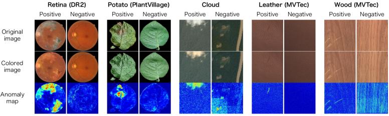
Figure 3: Examples of datasets. For each dataset, the original and colored image and the anomaly map calculated from the two images are shown for Positive and Negative.

4-1. Datasets

Datasets used here are shown in Fig. 3. We performed the experiment for image anomaly detection using DR2 (Pires et al. 2016), PlantVillage (Hughes and Salathe 2016), MVTec (Bergmann et al. 2019), and Cloud (Srinivas 2020) datasets. DR2 contains $435$ publicly available retina images with sizes of $857$ pixels. It consists of normal (negative) and Diabetic Retinopathy (positive) instances. PlantVillage contains images of healthy and diseased leaves of several plants. Among them, we used Potato dataset here. MVTec AD contains defect-free and anomalous images of various objects and texture categories. From this dataset, we used Leather and Wood, whose anomalies are strongly reflected in color. Cloud dataset contains images without clouds (negative) and with clouds (positive). The lowest panels in Fig. 3 represent anomaly maps. We see that anomalous regions in the Positive images were failed to reconstruct and highlighted in the color anomaly maps. All images were resized to $256\times 256$ pixels before experiments. To evaluate the performance on such practical dataset, we randomly extracted images from each dataset to construct imbalanced datasets. The details of datasets are shown in Table 2.

Table 2: Imbalanced experimental datasets reconstructed by random sampling.

Dataset Name	Positive	Negative	P to N Ratio	Total
Retina (DR2)	98	337	0.291	435
Potato (PlantVillage)	50	152	0.329	202
Cloud	100	300	0.333	400
Leather (MVTec)	92	277	0.332	369
Wood (MVTec)	60	266	0.226	326

4-2. Experimental Setup

We briefly describe the experimental setup for training. Parameters of U-Net were optimized by Adam optimizer with a learning rate of $0.001$. Momentums were set to $\beta_{1}=0.9$ and $\beta_{2}=0.999$. The total number of iterations to update the parameters was $500$ epochs, and the batch size was set to $16$. To reduce the computational time, early stopping was used.

In the anomaly detection experiment, we performed stratified five-fold cross-validation on each dataset without data augmentation. Parameters of ResNet18 were optimized by Adam optimizer with a learning rate of $0.0001$ and those of VGG16 were optimized by Adam optimizer with a learning rate of $0.00001$. The total number of iterations to update the parameters was set to $100$ epochs, and the batch size was $16$. All computations were performed on a GeForce RTX 2028 Ti GPU based on a system running Python $3.6.9$ and CUDA $10.0.130$.

4-3. Performance on Anomaly Detection

In LEA-Net, the attention map is incorporated into the intermediate layers of ADN via CAAN, which is the main idea of the layer-wise external attention mechanism. To evaluate the effectiveness of our attention mechanism, we compared the anomaly detection performance of LEA-Net with several settings: (i) baseline models (ResNet18, RestNet50, VGG16 and VGG19), (ii) ADN that receives anomaly map as inputs (Anomaly Map input), (iii) ADN that receives 4-channel images consist of RGB images and anomaly maps as inputs (4ch input), (iv) ADN that receives attention maps generated from RGB images and anomaly maps according to Eq. 3 as inputs (Attentioned input), (v) ADN with the layer-wise external attention at the attention point without CAAN (Direct Attention).

The averages of $F_{1}$ scores with a standard deviation in each experiment are shown in Table 3. The best and second-best performances are emphasized by bold type. The values given in parentheses indicate attention point of the best $F_{1}$ score. As mentioned above, the layer-wise external attention was applied at only one point in each experiment although the ADN has five attention points. For $F_{1}$ scores of models with the layer-wise external attention, we described the result of the best attention point score.

The results in Table 3 clearly show that the layer-wise external attention mechanism consistently increased the $F_{1}$ scores. In most of the cases, the layer-wise external attention with CAAN demonstrated better performance compared to that without CAAN. Surprisingly, for Potato dataset, the layer-wise external attention increased the $F_{1}$ score of ResNet18 by $0.304$. However, the performances were comparatively low in cases where the anomaly map was directly incorporated into ADN. Interestingly, we must mention here that the most effective attention point disagrees depending on the models and datasets.

Table 3: Comparison of $F_{1}$ scores on Retina, Potato, Cloud, Leather, Wood datasets

ADN Model	Params	Retina	Potato	Cloud	Leather	Wood
ResNet18	11.2M	0.642 $\pm$ 0.097	0.767 $\pm$ 0.164	0.642 $\pm$ 0.081	0.756 $\pm$ 0.147	0.560 $\pm$ 0.230
ResNet50	23.6M	0.544 $\pm$ 0.155	0.425 $\pm$ 0.315	0.635 $\pm$ 0.147	0.631 $\pm$ 0.152	0.546 $\pm$ 0.146
ResNet18 (AnomalyMap input)	11.2M	0.412 $\pm$ 0.005	0.779 $\pm$ 0.181	0.476 $\pm$ 0.058	0.551 $\pm$ 0.300	0.329 $\pm$ 0.137
ResNet18 (4ch input)	11.2M	0.443 $\pm$ 0.054	0.850 $\pm$ 0.102	0.529 $\pm$ 0.050	0.883 $\pm$ 0.066	0.495 $\pm$ 0.322
ResNet18 (Attentioned input)	11.2M	0.616 $\pm$ 0.108	0.823 $\pm$ 0.157	0.532 $\pm$ 0.050	0.752 $\pm$ 0.035	0.544 $\pm$ 0.22
ResNet18 + Direct Attention	11.2M	0.718 $\pm$ 0.047(3)	0.884 $\pm$ 0.045(4)	0.670 $\pm$ 0.084(3)	0.823 $\pm$ 0.055(3)	0.697 $\pm$ 0.061(4)
ResNet18 + MobileNet-small CAAN	13.5M	0.707 $\pm$ 0.037(1)	0.870 $\pm$ 0.094(4)	0.707 $\pm$ 0.131(2)	0.826 $\pm$ 0.062(1)	0.719 $\pm$ 0.247(2)
ResNet18 + ResNet-based CAAN	16.1M	0.737 $\pm$ 0.045(1)	0.948 $\pm$ 0.039(4)	0.664 $\pm$ 0.067(4)	0.828 $\pm$ 0.052(4)	0.621 $\pm$ 0.142(1)
VGG16	165.7M	0.709 $\pm$ 0.119	0.906 $\pm$ 0.061	0.575 $\pm$ 0.046	0.862 $\pm$ 0.089	0.652 $\pm$ 0.142
VGG19	171.0M	0.692 $\pm$ 0.068	0.941 $\pm$ 0.04	0.794 $\pm$ 0.041	0.758 $\pm$ 0.08	0.597 $\pm$ 0.338
VGG16 (AnomalyMap input)	165.7M	0.399 $\pm$ 0.012	0.899 $\pm$ 0.093	0.438 $\pm$ 0.023	0.907 $\pm$ 0.039	0.397 $\pm$ 0.111
VGG16 (4ch input)	165.7M	0.458 $\pm$ 0.031	0.823 $\pm$ 0.073	0.479 $\pm$ 0.092	0.925 $\pm$ 0.033	0.575 $\pm$ 0.042
VGG16 (Attentioned input)	165.7M	0.726 $\pm$ 0.056	0.947 $\pm$ 0.039	0.576 $\pm$ 0.119	0.877 $\pm$ 0.053	0.593 $\pm$ 0.269
VGG16 + Direct Attention	165.7M	0.754 $\pm$ 0.060(5)	0.927 $\pm$ 0.030(1)	0.596 $\pm$ 0.072(4)	0.877 $\pm$ 0.102(3)	0.746 $\pm$ 0.069(3)
VGG16 + MobileNet-small CAAN	168.0M	0.744 $\pm$ 0.068(3)	0.938 $\pm$ 0.058(1)	0.577 $\pm$ 0.069(3)	0.867 $\pm$ 0.077(2)	0.707 $\pm$ 0.074(4)
VGG16 + ResNet-based CAAN	170.6M	0.764 $\pm$ 0.069(5)	0.947 $\pm$ 0.064(1)	0.584 $\pm$ 0.076(5)	0.899 $\pm$ 0.091(3)	0.762 $\pm$ 0.035(5)

4-4. Performance on more imbalanced data

We conducted anomaly detection tests using more imbalanced datasets. Four datasets from Retina (DR2) and Potato (PlantVillage) were constructed by changing a proportion of the number of anomalous instances to that of all instances. Then, the performance of LEA-Net was compared to that of baseline models (ResNet18 and VGG16). Settings of LEA-Net were as follows: (i) ResNet18-based ADN with MobileNet-small CAAN, (ii) ResNet18-based ADN with ResNet-based CAAN, (iii) VGG16-based ADN with MobileNet-small CAAN, (iv) VGG16-based ADN with ResNet-based CAAN.

The resulting $F_{1}$ scores for each imbalanced dataset are described in Table 4. The upper two panels show the results for Retina and the lower two panels show those for Potato. All $F_{1}$ scores were averaged over the five-fold cross-validation. Horizontal axes indicate a proportion of the number of anomalous instances to that of all instances. We see that $F_{1}$ scores of the ResNet18-based ADN with CAAN were significantly improved by the layer-wise external attention throughout all imbalanced settings. Also, $F_{1}$ scores of VGG16-based ADN with CAAN for Potato were successfully improved in settings of $24.8\%$ and $12.4\%$. However, for $F_{1}$ scores of VGG16-based ADN with CAAN for Retina, there was no meaningful improvement in all settings.

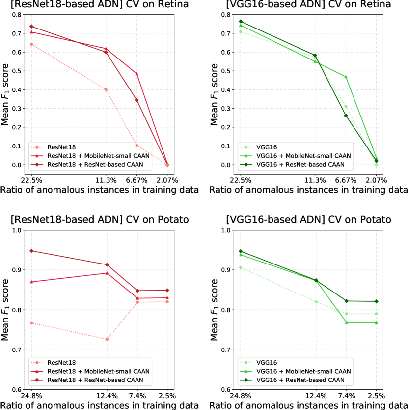
Figure 4: Performances on several imbalanced settings.

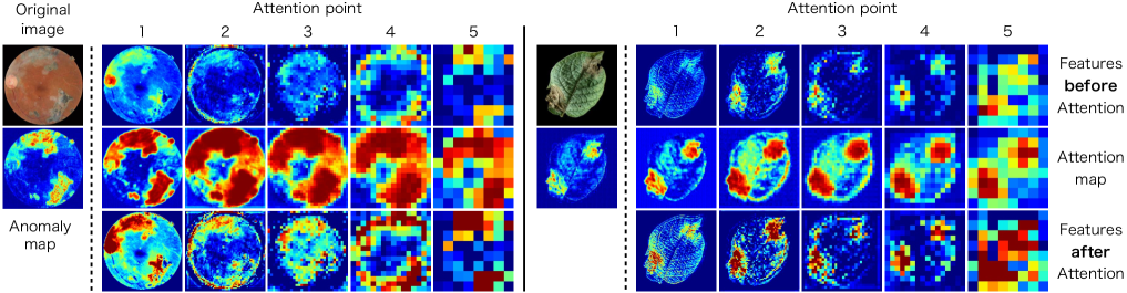
Figure 5: Visualization of feature maps at attention points before and after the layer-wise external attention.

4-5. Visualization of Attention Effects

Finally, we attempted to visualize how the layer-wise external attention induces attentions of ADN. Fig.5 displays feature maps output from intermediate layers in ResNet18-based ADN with ResNet-based CAAN before and after the layer-wise external attention for DR2 (Retina) and PlantVillage (Potato) datasets. We can see that anomalous regions were substantially highlighted by the layer-wise external attention throughout, from low-level to high-level features.

5. Conclusion

We proposed a Layer-wise External Attention Network (LEA-Net) for efficient image anomaly detection. LEA-Net has the layer-wise external attention mechanism to introduce prior knowledge about anomalies, represented as the anomaly map. Through experiments using real-world datasets including PlantVillage, MVTec AD, and Cloud datasets, we demonstrated that the proposed layer-wise external attention mechanism consistently boosts the anomaly detection performance of baseline models. We also confirmed that boosting abilities can remain even for significantly imbalanced datasets. For intuitive understanding of the proposed attention mechanism, we visualized and compared feature maps output from intermediate layers in Anomaly Detection Network (ADN) before and after layer-wise external attention. The results displayed that attention maps generated from Color Anomaly Attention Network (CAAN) successfully highlighted anomalous regions.

In this paper, we experimentally demonstrated that our new attention mechanism considerably boosts the anomaly detection performance of CNN-based image classifiers. We conclude that the layer-wise external attention is a promising technique for practical image anomaly detection. Moreover, we would like to emphasize that the technique is applicable not only for image anomaly detection, but also for various image recognition tasks. While, we found that the appropriate setting for successful boosting depends on the model and the dataset. Further studies focusing on theoretical aspects are expected to control adequately the layer-wise external attention.

Additional Experiment for Anomaly Detection

We performed additional experiments to evaluate the performance of LEA-Net using Hurricane (Mader 2019), Concrete (Zhang et al. 2016), PlantVillage (Hughes and Salathe 2016), MVTec (Bergmann et al. 2019), Cloud (Srinivas 2020) datasets. In the experiments, we additionally evaluate our layer-wise external attention on basic small CNN to see the effectiveness for various types of models. These experimental results were omitted from the main body of this paper due to the space constraints.

Additional Datasets

From PlantVillage, we used Grape and Strawberry datasets. From MVTec AD, we used Hazelnut, Tile and Carpet, which contain color anomalous instances. Hurricane dataset contains normal (negative) images and anomalous (positive) images. The anomalous images show damages caused by hurricanes such as floods. Concrete dataset contains normal images without damage and anomalous images with cracks and splits. All images were resized to $256\times 256$ pixels before experiments. The details of datasets are shown in Table 4 and Fig. 6.

In Fig. 6, we display illustrative examples of images and color anomaly maps for the dataset described above. The first rows show original color images. The second rows show reconstructed color images. The third rows show anomaly maps. Anomalous regions in the positive images are failed to be colored, and the regions are highlighted in the color anomaly maps.

Performance on Anomaly Detection

We show the comparison of anomaly detection performance between LEA-Net and other networks in Table 5-8. The performances are evaluated on the averages of $F_{1}$ scores with standard deviation. The best and second-best performances are emphasized by bold type. The values given in parentheses indicate attention point of the best $F_{1}$ score.

Table 5 and Table 6 show that LEA-Nets (networks with MobileNet-small or ResNet-based CAAN) demonstrated the best or second-best performances in most of the cases. From these results, it is shown that the layer-wise external attention mechanism consistently boosted the anomaly detection performances of ResNet18 and VGG16. In addition, Table 7 and Table 8 clearly show that the layer-wise external attention mechanism works well for basic CNN. The $F_{1}$ scores of basic CNN based LEA-Net are the hignest or second highest for most of datasets. From this additional experimental results, we confirmed that the layer-wise external attention mechanism is applicable and effective for various types of models.

Table 4: Additional experimental datasets.

Dataset Name	Positive	Negative	P to N Ratio	Total
Hurricane	100	300	0.333	400
Concrete	100	300	0.333	400
Grape	141	423	0.333	564
Strawberry	152	456	0.333	608
Tile	84	263	0.319	347
Hazelnut	70	431	0.162	501
Carpet	89	308	0.289	397

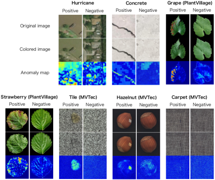
Figure 6: Examples of color anomaly maps for additional datasets. For each dataset, the original and colored image and the anomaly map calculated from the two images are shown for Positive and Negative instances. Anomalous regions in the Positive images are failed to be colored, and the regions are highlighted in the color anomaly maps.

Table 5: Comparison of $F_{1}$ scores on Hurricane, Concrete, Grape and Strawberry datasets.

Model	Params	Hurricane	Concrete	Grape	Strawberry
ResNet18	11.2M	0.874 $\pm$ 0.075	0.974 $\pm$ 0.026	0.944 $\pm$ 0.044	0.840 $\pm$ 0.197
ResNet50	23.6M	0.781 $\pm$ 0.125	0.921 $\pm$ 0.026	0.892 $\pm$ 0.062	0.820 $\pm$ 0.163
ResNet18 (AnomalyMap input)	11.2M	0.403 $\pm$ 0.007	0.790 $\pm$ 0.218	0.856 $\pm$ 0.133	0.778 $\pm$ 0.226
ResNet18 (4ch input)	11.2M	0.412 $\pm$ 0.013	0.946 $\pm$ 0.035	0.918 $\pm$ 0.027	0.866 $\pm$ 0.137
ResNet18 (Attentioned input)	11.2M	0.500 $\pm$ 0.076	0.952 $\pm$ 0.029	0.895 $\pm$ 0.101	0.899 $\pm$ 0.095
ResNet18 + Direct Attention	11.2M	0.870 $\pm$ 0.058(5)	0.963 $\pm$ 0.036(5)	0.951 $\pm$ 0.046(1)	0.986 $\pm$ 0.019(2)
ResNet18 + MobileNet-small CAAN	13.5M	0.858 $\pm$ 0.076(3)	0.979 $\pm$ 0.029(1)	0.978 $\pm$ 0.039(4)	0.987 $\pm$ 0.022(4)
ResNet18 + ResNet-based CAAN	16.1M	0.866 $\pm$ 0.054(5)	0.969 $\pm$ 0.022(3)	0.961 $\pm$ 0.048(2)	0.957 $\pm$ 0.054(3)
VGG16	165.7M	0.702 $\pm$ 0.092	0.959 $\pm$ 0.029	0.982 $\pm$ 0.026	0.959 $\pm$ 0.033
VGG19	171.0M	0.655 $\pm$ 0.065	0.980 $\pm$ 0.011	0.971 $\pm$ 0.016	0.963 $\pm$ 0.03
VGG16 (AnomalyMap input)	165.7M	0.400 $\pm$ 0.000	0.886 $\pm$ 0.028	0.902 $\pm$ 0.051	0.849 $\pm$ 0.109
VGG16 (4ch input)	165.7M	0.441 $\pm$ 0.034	0.942 $\pm$ 0.036	0.956 $\pm$ 0.037	0.765 $\pm$ 0.158
VGG16 (Attentioned input)	165.7M	0.584 $\pm$ 0.119	0.938 $\pm$ 0.047	0.978 $\pm$ 0.015	0.966 $\pm$ 0.025
VGG16 + Direct Attention	165.7M	0.717 $\pm$ 0.029(5)	0.969 $\pm$ 0.021(5)	0.982 $\pm$ 0.013(3)	0.968 $\pm$ 0.039(1)
VGG16 + MobileNet-small CAAN	168.0M	0.715 $\pm$ 0.084(5)	0.964 $\pm$ 0.023(1)	0.986 $\pm$ 0.015(1)	0.969 $\pm$ 0.027(3)
VGG16 + ResNet-based CAAN	170.6M	0.725 $\pm$ 0.045(4)	0.964 $\pm$ 0.023(3)	0.986 $\pm$ 0.015(1)	0.973 $\pm$ 0.020(2)

Table 6: Comparison of $F_{1}$ scores on Tile, Hazelnut and Carpet datasets.

Model	Params	Tile	Hazelnut	Carpet
ResNet18	11.2M	0.768 $\pm$ 0.120	0.866 $\pm$ 0.021	0.711 $\pm$ 0.061
ResNet50	23.6M	0.601 $\pm$ 0.228	0.779 $\pm$ 0.302	0.524 $\pm$ 0.151
ResNet18 (AnomalyMap input)	11.2M	0.381 $\pm$ 0.103	0.635 $\pm$ 0.06	0.392 $\pm$ 0.195
ResNet18 (4ch input)	11.2M	0.669 $\pm$ 0.190	0.854 $\pm$ 0.193	0.686 $\pm$ 0.06
ResNet18 (Attentioned input)	11.2M	0.750 $\pm$ 0.136	0.787 $\pm$ 0.304	0.735 $\pm$ 0.057
ResNet18 + Direct Attention	11.2M	0.780 $\pm$ 0.077(5)	0.902 $\pm$ 0.075(1)	0.756 $\pm$ 0.045(3)
ResNet18 + MobileNet-small CAAN	13.5M	0.789 $\pm$ 0.096(2)	0.919 $\pm$ 0.079(2)	0.788 $\pm$ 0.057(3)
ResNet18 + ResNet-based CAAN	16.1M	0.776 $\pm$ 0.103(3)	0.897 $\pm$ 0.040(5)	0.724 $\pm$ 0.055(1)
VGG16	165.7M	0.346 $\pm$ 0.094	0.857 $\pm$ 0.082	0.373 $\pm$ 0.349
VGG19	171.0M	0.835 $\pm$ 0.091	0.903 $\pm$ 0.057	0.634 $\pm$ 0.304
VGG16 (AnomalyMap input)	165.7M	0.599 $\pm$ 0.115	0.7 $\pm$ 0.092	0.423 $\pm$ 0.177
VGG16 (4ch input)	165.7M	0.589 $\pm$ 0.103	0.78 $\pm$ 0.129	0.593 $\pm$ 0.137
VGG16 (Attentioned input)	165.7M	0.512 $\pm$ 0.134	0.791 $\pm$ 0.074	0.252 $\pm$ 0.141
VGG16 + Direct Attention	165.7M	0.399 $\pm$ 0.103(2)	0.842 $\pm$ 0.068(3)	0.479 $\pm$ 0.108(3)
VGG16 + MobileNet-small CAAN	168.0M	0.432 $\pm$ 0.177(2)	0.828 $\pm$ 0.066(4)	0.55 $\pm$ 0.186(4)
VGG16 + ResNet-based CAAN	170.6M	0.525 $\pm$ 0.128(1)	0.82 $\pm$ 0.057(1)	0.484 $\pm$ 0.247(4)

Table 7: Comparison of $F_{1}$ scores on Retina, Potato, Cloud and Leather datasets.

Model	Params	Retina	Potato	Cloud	Leather
basic CNN	4.0M	0.621 $\pm$ 0.027	0.868 $\pm$ 0.066	0.276 $\pm$ 0.131	0.54 $\pm$ 0.094
basic CNN (AnomalyMap input)	4.0M	0.417 $\pm$ 0.036	0.772 $\pm$ 0.018	0.475 $\pm$ 0.056	0.45 $\pm$ 0.191
basic CNN (4ch input)	4.0M	0.483 $\pm$ 0.052	0.829 $\pm$ 0.064	0.421 $\pm$ 0.057	0.613 $\pm$ 0.111
basic CNN (Attentioned input)	4.0M	0.63 $\pm$ 0.049	0.858 $\pm$ 0.058	0.383 $\pm$ 0.109	0.459 $\pm$ 0.087
basic CNN + Direct Attention	4.0M	0.65 $\pm$ 0.055(3)	0.884 $\pm$ 0.051(5)	0.332 $\pm$ 0.103(3)	0.625 $\pm$ 0.11(5)
basic CNN + MobileNet-small CAAN	7.0M	0.652 $\pm$ 0.015(5)	0.925 $\pm$ 0.033(5)	0.324 $\pm$ 0.09(4)	0.606 $\pm$ 0.093(3)
basic CNN + ResNet-based CAAN	8.9M	0.654 $\pm$ 0.052(3)	0.907 $\pm$ 0.074(4)	0.337 $\pm$ 0.111(4)	0.591 $\pm$ 0.134(4)

Table 8: Comparison of $F_{1}$ scores on Hurricane, Concrete, Grape and Hazelnut datasets.

Model	Params	Hurricane	Concrete	Grape	Hazelnut
basic CNN	4.0M	0.835 $\pm$ 0.072	0.875 $\pm$ 0.071	0.955 $\pm$ 0.017	0.463 $\pm$ 0.172
basic CNN (AnomalyMap input)	4.0M	0.401 $\pm$ 0.002	0.795 $\pm$ 0.109	0.868 $\pm$ 0.1	0.503 $\pm$ 0.183
basic CNN (4ch input)	4.0M	0.44 $\pm$ 0.024	0.888 $\pm$ 0.055	0.917 $\pm$ 0.074	0.683 $\pm$ 0.137
basic CNN (Attentioned input)	4.0M	0.601 $\pm$ 0.18	0.882 $\pm$ 0.057	0.941 $\pm$ 0.03	0.377 $\pm$ 0.231
basic CNN + Direct Attention	4.0M	0.848 $\pm$ 0.072(3)	0.905 $\pm$ 0.049(3)	0.96 $\pm$ 0.024(3)	0.465 $\pm$ 0.151(4)
basic CNN + MobileNet-small CAAN	7.0M	0.847 $\pm$ 0.089(4)	0.918 $\pm$ 0.062(5)	0.956 $\pm$ 0.017(2)	0.462 $\pm$ 0.166(4)
basic CNN + ResNet-based CAAN	8.9M	0.863 $\pm$ 0.101(2)	0.924 $\pm$ 0.051(5)	0.959 $\pm$ 0.029(4)	0.545 $\pm$ 0.261(5)

U-Net Architecture

In Table  9, we describe the architecture of U-Net that was used in the color anomaly map generation step. The sizes of input images are $256\times 256$ pixels, and there are eight downsampling points. Except for the first and the last convolutional and deconvolutional layers, batch normalization layers are followed by the convolutional and the deconvolutional layers.

Table 9: The U-Net architecture used in the present study. Conv2D denotes a 2D convolutional layer and BN denotes a batch normalization. All alpha values of LeakyRelu are $0.2$.

ID	Layer Type	Output dim	Kernel	Stride	Filters	Activation
1	Input	256 $\times$ 256	-	-	-	-
2	Conv2D	128 $\times$ 128	4	2	64	LeakyRelu
3	Conv2D $\rightarrow$ BN	64 $\times$ 64	4	2	128	LeakyRelu
4	Conv2D $\rightarrow$ BN	32 $\times$ 32	4	2	256	LeakyRelu
5	Conv2D $\rightarrow$ BN	16 $\times$ 16	4	2	512	LeakyRelu
6	Conv2D $\rightarrow$ BN	8 $\times$ 8	4	2	512	LeakyRelu
7	Conv2D $\rightarrow$ BN	4 $\times$ 4	4	2	512	LeakyRelu
8	Conv2D $\rightarrow$ BN	2 $\times$ 2	4	2	512	LeakyRelu
9	Conv2D $\rightarrow$ BN	1 $\times$ 1	4	2	512	LeakyRelu
10	Conv2DTranspose$\rightarrow$ BN	2 $\times$ 2	2	2	512	Relu
11	Concat(8, 10)	2 $\times$ 2	-	-	1024	-
12	Conv2DTranspose$\rightarrow$ BN	4 $\times$ 4	2	2	512	Relu
13	Concat(7, 12)	4 $\times$ 4	-	-	1024	-
14	Conv2DTranspose$\rightarrow$ BN	8 $\times$ 8	2	2	512	Relu
15	Concat(6, 14)	8 $\times$ 8	-	-	1024	-
16	Conv2DTranspose$\rightarrow$ BN	16 $\times$ 16	2	2	512	Relu
17	Concat(5, 16)	16 $\times$ 16	-	-	1024	-
18	Conv2DTranspose$\rightarrow$ BN	32 $\times$ 32	2	2	256	Relu
19	Concat(4, 18)	32 $\times$ 32	-	-	512	-
20	Conv2DTranspose$\rightarrow$ BN	64 $\times$ 64	2	2	128	Relu
21	Concat(3, 20)	64 $\times$ 64	-	-	256	-
22	Conv2DTranspose$\rightarrow$ BN	128 $\times$ 128	2	2	64	Relu
23	Concat(2, 22)	128 $\times$ 128	-	-	128	-
24	Conv2DTranspose	256 $\times$ 256	2	2	2	sigmoid

References

- Akcay, Atapour-Abarghouei, and Breckon (2018) Akcay, S.; Atapour-Abarghouei, A.; and Breckon, T. P. 2018. GANomaly: semi-supervised anomaly detection via adversarial training.
- Bergmann et al. (2019) Bergmann, P.; Fauser, M.; Sattlegger, D.; and Steger, C. 2019. MVTec AD — A Comprehensive Real-World Dataset for Unsupervised Anomaly Detection. In 2019 IEEE/CVF Conference on Computer Vision and Pattern Recognition (CVPR).
- Cao et al. (2018) Cao, C.; Liu, F.; Tan, H.; Song, D.; Shu, W.; Li, W.; Zhou, Y.; Bo, X.; and Xie, Z. 2018. Deep learning and its applications in biomedicine. Genomics, proteomics & bioinformatics, 16(1): 17–32.
- Chun, Golomb, and Turk-Browne (2011) Chun, M. M.; Golomb, J. D.; and Turk-Browne, N. B. 2011. A taxonomy of external and internal attention. Annual review of psychology, 62: 73–101.
- Emami et al. (2020) Emami, H.; Aliabadi, M. M.; Dong, M.; and Chinnam, R. B. 2020. Spa-gan: Spatial attention gan for image-to-image translation. IEEE Transactions on Multimedia, 23: 391–401.
- Ferentinos (2018) Ferentinos, K. P. 2018. Deep learning models for plant disease detection and diagnosis. Computers and Electronics in Agriculture, 145: 311–318.
- Fukui et al. (2019) Fukui, H.; Hirakawa, T.; Yamashita, T.; and Fujiyoshi, H. 2019. Attention Branch Network: Learning of Attention Mechanism for Visual Explanation. arXiv:1812.10025.
- Goernitz et al. (2013) Goernitz, N.; Kloft, M.; Rieck, K.; and Brefeld, U. 2013. Toward Supervised Anomaly Detection. Journal of Artificial Intelligence Research, 46: 235–262.
- Haselmann, Gruber, and Tabatabai (2018) Haselmann, M.; Gruber, D. P.; and Tabatabai, P. 2018. Anomaly Detection using Deep Learning based Image Completion. arXiv:1811.06861.
- He et al. (2016) He, K.; Zhang, X.; Ren, S.; and Sun, J. 2016. Deep residual learning for image recognition. In Proceedings of the IEEE conference on computer vision and pattern recognition, 770–778.
- Hinton, Vinyals, and Dean (2015) Hinton, G.; Vinyals, O.; and Dean, J. 2015. Distilling the Knowledge in a Neural Network. arXiv:1503.02531.
- Howard et al. (2019) Howard, A.; Sandler, M.; Chu, G.; Chen, L.-C.; Chen, B.; Tan, M.; Wang, W.; Zhu, Y.; Pang, R.; Vasudevan, V.; Le, Q. V.; and Adam, H. 2019. Searching for MobileNetV3. arXiv:1905.02244.
- Hu et al. (2020) Hu, J.; Shen, L.; Albanie, S.; Sun, G.; and Wu, E. 2020. Squeeze-and-Excitation Networks. IEEE Transactions on Pattern Analysis and Machine Intelligence, 42(8): 2011–2023.
- Hughes and Salathe (2016) Hughes, D. P.; and Salathe, M. 2016. An open access repository of images on plant health to enable the development of mobile disease diagnostics.
- Katafuchi and Tokunaga (2021) Katafuchi, R.; and Tokunaga, T. 2021. Image-based Plant Disease Diagnosis with Unsupervised Anomaly Detection based on Reconstructability of Colors. 112–120.
- Krizhevsky, Sutskever, and Hinton (2012) Krizhevsky, A.; Sutskever, I.; and Hinton, G. E. 2012. Imagenet classification with deep convolutional neural networks. Advances in neural information processing systems, 25: 1097–1105.
- Lee, Kim, and Nam (2019) Lee, H.; Kim, H. E.; and Nam, H. 2019. SRM: A style-based recalibration module for convolutional neural networks. Proceedings of the IEEE International Conference on Computer Vision, 2019-Octob: 1854–1862.
- Li et al. (2021) Li, W.; Cheng, S.; Qian, K.; Yue, K.; and Liu, H. 2021. Automatic Recognition and Classification System of Thyroid Nodules in CT Images Based on CNN. Computational Intelligence and Neuroscience, 2021.
- Lu (2020) Lu, L. 2020. Dying ReLU and Initialization: Theory and Numerical Examples. Communications in Computational Physics, 28(5): 1671–1706.
- Mader (2019) Mader, K. 2019. Satellite Images of Hurricane Damage. https://www.kaggle.com/kmader/satellite-images-of-hurricane-damage. Accessed: 2020-11-11.
- Minhas and Zelek (2019) Minhas, M. S.; and Zelek, J. 2019. Anomaly detection in images. arXiv preprint arXiv:1905.13147.
- Natarajan, Mao, and Chia (2019) Natarajan, V.; Mao, S.; and Chia, L.-T. 2019. Salient Textural Anomaly Proposals and Classification for Metal Surface Anomalies. In 2019 IEEE 31st International Conference on Tools with Artificial Intelligence (ICTAI), 621–628.
- Pires et al. (2016) Pires, R.; Jelinek, H. F.; Wainer, J.; Valle, E.; and Rocha, A. 2016. Advancing Bag-of-Visual-Words Representations for Lesion Classification in Retinal Images.
- Reynolds and Chelazzi (2004) Reynolds, J. H.; and Chelazzi, L. 2004. Attentional modulation of visual processing. Annu. Rev. Neurosci., 27: 611–647.
- Rezvantalab, Safigholi, and Karimijeshni (2018) Rezvantalab, A.; Safigholi, H.; and Karimijeshni, S. 2018. Dermatologist level dermoscopy skin cancer classification using different deep learning convolutional neural networks algorithms. arXiv preprint arXiv:1810.10348.
- Ronneberger, Fischer, and Brox (2015) Ronneberger, O.; Fischer, P.; and Brox, T. 2015. U-net: Convolutional networks for biomedical image segmentation. In International Conference on Medical image computing and computer-assisted intervention, 234–241. Springer.
- Schlegl et al. (2017) Schlegl, T.; Seebock, P.; Waldstein, S. M.; Schmidt-Erfurth, U.; and Langs, G. 2017. Unsupervised anomaly detection with Generative Adversarial Networks to guide marker discovery. In International Conference on Information Processing in Medical Imaging, 146–157.
- Sharma, Wu, and Dalal (2005) Sharma, G.; Wu, W.; and Dalal, E. N. 2005. The CIEDE2000 color-difference formula: implementation notes, supplementary test data, and mathematical observations. Color Research and Application, 30(1).
- Srinivas (2020) Srinivas, A. 2020. Cloud and Non-Cloud Images (Anomaly Detection). https://www.kaggle.com/ashoksrinivas/cloud-anomaly-detection-images. Accessed: 2020-08-22.
- Venkataramanan et al. (2020) Venkataramanan, S.; Peng, K.-C.; Singh, R. V.; and Mahalanobis, A. 2020. Attention guided anomaly localization in images. In European Conference on Computer Vision, 485–503. Springer.
- Wang et al. (2017) Wang, F.; Jiang, M.; Qian, C.; Yang, S.; Li, C.; Zhang, H.; Wang, X.; and Tang, X. 2017. Residual attention network for image classification. Proceedings - 30th IEEE Conference on Computer Vision and Pattern Recognition, CVPR 2017, 2017-Janua(1): 6450–6458.
- Wang et al. (2020) Wang, Q.; Wu, B.; Zhu, P.; Li, P.; Zuo, W.; and Hu, Q. 2020. ECA-Net: Efficient channel attention for deep convolutional neural networks. Proceedings of the IEEE Computer Society Conference on Computer Vision and Pattern Recognition, 11531–11539.
- Woo et al. (2018) Woo, S.; Park, J.; Lee, J. Y.; and Kweon, I. S. 2018. CBAM: Convolutional block attention module. Lecture Notes in Computer Science (including subseries Lecture Notes in Artificial Intelligence and Lecture Notes in Bioinformatics), 11211 LNCS: 3–19.
- Yang et al. (2021) Yang, L.; Zhang, R.-Y.; Li, L.; and Xie, X. 2021. SimAM: A Simple, Parameter-Free Attention Module for Convolutional Neural Networks. In International Conference on Machine Learning, 11863–11874. PMLR.
- Zagoruyko and Komodakis (2017) Zagoruyko, S.; and Komodakis, N. 2017. Paying more attention to attention: Improving the performance of convolutional neural networks via attention transfer. 5th International Conference on Learning Representations, ICLR 2017 - Conference Track Proceedings, 1–13.
- Zenati et al. (2018) Zenati, H.; Foo, C.-S.; Lecouat, B.; Manek, G.; and Chandrasekhar, V. R. 2018. Efficient GAN-Based anomaly detection. In 6th International Conference on Learning Representations (ICLR2018).
- Zhang et al. (2016) Zhang, L.; Yang, F.; Daniel Zhang, Y.; and Zhu, Y. J. 2016. Road crack detection using deep convolutional neural network. In 2016 IEEE International Conference on Image Processing (ICIP), 3708–3712.
- Zhao, Jia, and Koltun (2020) Zhao, H.; Jia, J.; and Koltun, V. 2020. Exploring Self-attention for Image Recognition. Proceedings of the IEEE Computer Society Conference on Computer Vision and Pattern Recognition, 10073–10082.