Exploring Task Difficulty for Few-Shot Relation Extraction

Abstract

Few-shot relation extraction (FSRE) focuses on recognizing novel relations by learning with merely a handful of annotated instances. Meta-learning has been widely adopted for such a task, which trains on randomly generated few-shot tasks to learn generic data representations. Despite impressive results achieved, existing models still perform suboptimally when handling hard FSRE tasks, where the relations are fine-grained and similar to each other. We argue this is largely because existing models do not distinguish hard tasks from easy ones in the learning process. In this paper, we introduce a novel approach based on contrastive learning that learns better representations by exploiting relation label information. We further design a method that allows the model to adaptively learn how to focus on hard tasks. Experiments on two standard datasets demonstrate the effectiveness of our method.

1 Introduction

Relation extraction aims to detect the relation between two entities contained in a sentence, which is the cornerstone of various natural language processing (NLP) applications, including knowledge base enrichment Trisedya et al. (2019), biomedical knowledge discovery Guo et al. (2020), and question answering Han et al. (2020). Conventional neural methods Miwa and Bansal (2016); Tran et al. (2019) train a deep network through a large amount of labeled data with extensive relations, so that the model can recognize these relations during the test phase. Although impressive performance has been achieved, these methods are difficult to adapt to novel relations that have never been seen in the training process. In contrast, humans can identify new relations with very few examples. It is thus of great interest to enable the model to generalize to new relations with a handful of labeled instances.

Inspired by the success of few-shot learning in the computer vision (CV) community Sung et al. (2018); Satorras and Estrach (2018), Han et al. (2018) first introduce the task of few-shot relation extraction (FSRE). FSRE requires models to be capable of handling classification of novel relations with scarce labeled instances. A popular framework for few-shot learning is meta-learning Santoro et al. (2016); Vinyals et al. (2016), which optimizes the model through collections of few-shot tasks sampled from the external data containing disjoint relations with novel relations, so that the model can learn cross-task knowledge and use the knowledge to acclimate rapidly to new tasks. A simple yet effective algorithm based on meta-learning is prototypical network (Snell et al., 2017), aiming to learn a metric space in which a query instance is classified according to its distance to class prototypes. Recently, many works Gao et al. (2019a); Qu et al. (2020); Yang et al. (2020) for FSRE are in line with prototypical networks, which achieve remarkable performance. Nonetheless, the difficulty of distinguishing relations varies in different tasks Zhou et al. (2020), depending on the similarity between relations. As illustrated in Figure LABEL:intro, there are easy few-shot tasks whose relations are quite different, so that they can be consistently well-classified, and also hard few-shot tasks with subtle inter-relation variations which are prone to misclassification. Current FSRE methods struggle with handling the hard tasks given limited labeled instances due to two main reasons. First, most works mainly focus on general tasks to learn generalized representations, and ignore modeling subtle and local differences of relations effectively, which may hinder these models from dealing with hard tasks well. Second, current meta-learning methods treat training tasks equally, which are randomly sampled and have different degrees of difficulty. The generated easy tasks can overwhelm the training process training and lead to a degenerate model.

To fill this gap, this paper proposes a Hybrid Contrastive Relation-Prototype (HCRP) approach, which focuses on improving the performance on hard FSRE tasks. Concretely, we first propose a hybrid prototypical network, capable of capturing global and local features to generate the informative class prototypes. Next, we present a novel relation-prototype contrastive learning method, which leverages relation descriptions as anchors, and pulls the prototype of the same class closer in representation space and pushes those of different classes away. In this way, the model gains diverse and discriminative prototype representations, which could be beneficial to distinguish the subtle difference of confusing relations in hard few-shot tasks. Furthermore, we design a task-adaptive training strategy based on focal loss (Lin et al., 2017) to learn more from hard tasks, which allocates dynamic weights to different tasks according to task difficulty. Extensive experiments on two large-scale benchmarks show that our model significantly outperforms the baselines. Ablation and case studies demonstrate the effectiveness of the proposed modules. Our code is available at https://github.com/hanjiale/HCRP .

The contributions of this paper are summarized as follows:

• We present HCRP to explore task difficulty as useful information for FSRE, which boosts hybrid prototypical network with relation-prototype contrastive learning to capture diverse and discriminative representations.

• We design a novel task adaptive focal loss to focus training on hard tasks, which enables the model to achieve higher robustness and better performance.

• Qualitative and quantitative experiments on two FSRE benchmarks demonstrate the effectiveness of our model.

2 Related Work

2.1 Few-shot Relation Extraction

Relation extraction is a foundational and important task in NLP and attracts many recent attentions Nan et al. (2020); Chen et al. (2021). Few-shot relation extraction aims to predict novel relations by exploring a few labeled instances. Han et al. (2018) first present a large-scale benchmark FewRel for FSRE. Gao et al. (2019a) design a hybrid attention-based prototypical network to highlight the crucial instances and features. Ye and Ling (2019) propose a prototypical network with multi-level matching and aggregation. Sun et al. (2019) present a hierarchical attention prototypical network to enhance the representation ability of semantic space. Qu et al. (2020) utilize an external relation graph to study the relationships between different relations. Wang et al. (2020) apply added relative position information and syntactic relation information to enhance prototypical networks. Yang et al. (2020) fuse text descriptions of relations and entities by a collaborative attention mechanism. And Yang et al. (2021) introduce the inherent concepts of entities to provide clues for relation classification. There are also some methods Baldini Soares et al. (2019); Peng et al. (2020) combining prototypical networks with pre-trained language models, which achieve impressive results. However, the task difficulty of FSRE has not been explored. In this work, we focus on the hard tasks and propose a hybrid contrastive relation-prototype method to better model subtle variations across different relations.

2.2 Contrastive Learning

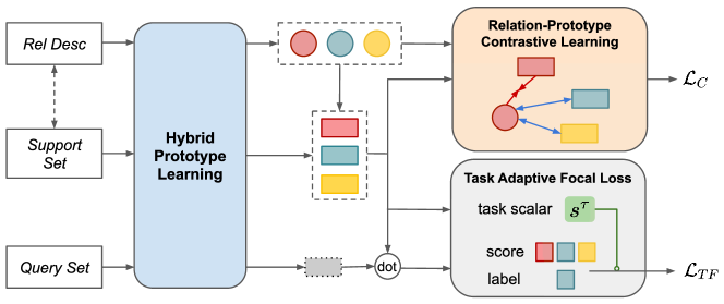
Figure 2: The overall framework of HCRP. Best viewed in color. The rectangles represent the class prototypes, the circles represent the relations, and different colors represent different classes.

Contrastive learning Jaiswal et al. (2021) has gained popularity recently in the CV community. The core idea is to contrast the similarities and dissimilarities between data instances, which pulls the positives closer and pushes negatives away simultaneously. CPC van den Oord et al. (2018) proposes a universal unsupervised learning approach. MoCo He et al. (2020) presents a mechanism for building dynamic dictionaries for contrastive learning. SimCLR Chen et al. (2020) improves contrastive learning by using larger batch size and data augmentation. Khosla et al. (2020) extend the self-supervised contrastive approach to the supervised setting. Nan et al. (2021) propose a dual contrastive learning approach for video grounding. There are also some applications of contrastive learning in the field of NLP. Fang and Xie (2020) employ back translation and MoCo to learn sentence-level representations. Gunel et al. (2021) design supervised contrastive learning for pre-trained language model fine-tuning. Inspired by these works, we propose a heterogeneous relation-prototype contrastive learning in a supervised way to obtain more discriminative representations.

3 Task Definition

We follow a typical few-shot task setting, namely the $N$-way-$K$-shot setup, which contains a support set $\mathcal{S}$ and a query set $\mathcal{Q}$. The support set $\mathcal{S}$ includes $N$ novel classes, each with $K$ labeled instances. The query set $\mathcal{Q}$ contains the same $N$ classes as $\mathcal{S}$. And the task is evaluated on query set $\mathcal{Q}$, trying to predict the relations of instances in $\mathcal{Q}$. What’s more, an auxiliary dataset $\mathcal{D}_{base}$ is given, which contains abundant base classes, each with a large number of labeled examples. Note the base classes and novel classes are disjoint with each other. The few-shot learner aims to acquire knowledge from base classes and use the knowledge to recognize novel classes. One popular approach is the meta-learning paradigm Vinyals et al. (2016), which mimics the few-shot learning settings at training stage. Specifically, in each training iteration, we randomly select $N$ classes from base classes, each with $K$ instances to form a support set $\mathcal{S}=\{s_{k}^{i};i=1,\dots,N,k=1,\dots,K\}$. Meanwhile, $R$ instances are sampled from the remaining data of the $N$ classes to construct a query set $\mathcal{Q}=\{q_{j};j=1,\dots,R\}$. The model is optimized by collections of few-shot tasks sampled from base classes, so that it can rapidly adapt to new tasks.

For an FSRE task, each instance consists of a set of samples $(x,e,y)$, where $x$ denotes a natural language sentence, $e=(e_{h},e_{t})$ indicates a pair of head entity and tail entity, and $y$ is the relation label. The name and description for each relation are also provided as auxiliary support evidence for relation extraction. For example, for a relation with its relation id “P726” in a dataset that we use, we can obtain its name “candidate” and description “person or party that is an option for an office in an election”.

4 Approach

In this section, we present the details of our proposed HCRP approach. The overall learning framework is illustrated in Figure 2. The inputs are $N$-way-$K$-shot tasks (sampled from the auxiliary dataset $\mathcal{D}_{base}$), where each task contains a support set $\mathcal{S}$ and a query set $\mathcal{Q}$. Meanwhile, we take the names and descriptions of these $N$ classes (i.e., relations) as inputs as well. HCRP consists of three components. The hybrid prototype learning module generates informative prototypes by capturing global and local features, which can better capture the subtle differences of relations. The relation-prototype contrastive learning component is then used to leverage the relation label information to further enhance the discriminative power of the prototype representations. Finally, a task adaptive focal loss is introduced to encourage the model to focus training on hard tasks.

4.1 Hybrid Prototype Learning

We employ BERT Devlin et al. (2019) as the encoder to obtain contextualized embeddings of query instances $\{\mathbf{Q}_{j}\in\mathbb{R}^{l_{q_{j}}\times d};j=1,\dots,R\}$ and support instances $\{\mathbf{S}_{k}^{i}\in\mathbb{R}^{l_{s_{k}^{i}}\times d};i=1,\dots,N,k=1,\dots,K\}$, where $l_{q_{j}}$ and $l_{s_{k}^{i}}$ are the sentence lengths of the $j$-th query instance and $k$-th support instance in class $i$ respectively, and $d$ is the size of the resulting contextualized representations. For each relation, we concatenate the name and description and feed the sequence into the BERT encoder to obtain relation embeddings $\{\mathbf{R}^{i}\in\mathbb{R}^{l_{r^{i}}\times d};i=1,\dots,N\}$, where $l_{r^{i}}$ is the length of relation description $i$.

Global Prototypes

For instances in $\mathcal{S}$ and $\mathcal{Q}$, the global features $\{\mathbf{s}_{k}^{i}\in\mathbb{R}^{2d};i=1,\dots,N,k=1,\dots,K\}$ and $\{\mathbf{q}_{j}\in\mathbb{R}^{2d};j=1,\dots,R\}$ are obtained by concatenating the hidden states corresponding to start tokens of two entity mentions following Baldini Soares et al. (2019). The global features of relations $\{\mathbf{r}^{i}\in\mathbb{R}^{2d};i=1,\dots,N\}$ are obtained by the hidden states corresponding to [CLS] token (converted to $2d$ dimension with a transformation). For each relation $i$, we average the global features of the $K$ supporting instances following the work of Snell et al. (2017), and further add the global feature of relation to form global prototype representation.

$$\mathbf{p}_{g}^{i}=\frac{1}{K}\sum_{k=1}^{K}\mathbf{s}_{k}^{i}+\mathbf{r}^{i}\in\mathbb{R}^{2d}$$ (1)

Local Prototypes

While global prototypes are capable of capturing general data representations, such representations may not readily capture useful local information within specific RSRE tasks. To better handle the hard FSRE tasks with subtle differences among highly similar relations, we further propose local prototypes to highlight key tokens in an instance that are essential to characterize different relations.

For relation $i$, we first calculate the local feature of the $k$-th support instance as:

$$\hat{\mathbf{s}}_{k}^{i} = \sum_{n=1}^{l_{s_{k}^{i}}}\alpha^{s}_{n}{[\mathbf{S}_{k}^{i}]}_{n}\in\mathbb{R}^{d}$$ (2)

$$\alpha^{s} = {\rm softmax}({\rm sum}(\mathbf{S}_{k}^{i}{(\mathbf{R}^{i})}^{\mathsf{T}}))\in\mathbb{R}^{l_{s_{k}^{i}}}$$ (3)

where ${[\cdot]}_{n}$ is the $n$-th row of a matrix, ${\rm sum}()$ is an operation that sums all elements for each row in a matrix. Specifically, we allocate weights to different tokens according to their similarities with relation descriptions, and take the weighted sum to form such local features.

Similarly, we calculate the similarity between relation embedding $\mathbf{R}^{i}$ and each support instance embedding $\mathbf{S}_{k}^{i}$ of relation $i$ and obtain $K$ features $\{\hat{\mathbf{r}}_{k}^{i};k=1,\dots,K\}$:

$$\hat{\mathbf{r}}_{k}^{i} = \sum_{n=1}^{l_{r^{i}}}\alpha^{r}_{n}[\mathbf{R}^{i}]_{n}\in\mathbb{R}^{d}$$ (4)

$$\alpha^{r} = {\rm softmax}({\rm sum}(\mathbf{R}^{i}{(\mathbf{S}_{k}^{n})}^{\mathsf{T}}))\in\mathbb{R}^{l_{r^{i}}}$$ (5)

The $K$ features are then averaged to arrive at the final local representation of relation $i$:

$$\hat{\mathbf{r}}^{i}=\frac{1}{K}\sum_{k=1}^{K}\hat{\mathbf{r}}_{k}^{i}\in\mathbb{R}^{d}$$ (6)

The local feature of a query instance is calculated by the following formulas.

$$\hat{\mathbf{q}}_{j} = \sum_{n=1}^{l_{q_{j}}}\alpha^{q}_{n}{[\mathbf{Q}_{j}]}_{n}\in\mathbb{R}^{d}$$ (7)

$$\alpha^{q} = {\rm softmax}({\rm sum}(\mathbf{Q}_{j}\mathbf{Q}_{j}^{\mathsf{T}}))\in\mathbb{R}^{l_{q_{j}}}$$ (8)

Finally, we generate the local prototype by averaging the local features of the support set, plus the local feature of the relation.

$$\mathbf{p}_{l}^{i}=\frac{1}{K}\sum_{k=1}^{K}\hat{\mathbf{s}}_{k}^{i}+\hat{\mathbf{r}}^{i}\in\mathbb{R}^{d}$$ (9)

Hybrid Prototypes

The model concatenates the global and local prototype to form hybrid prototype representations:

$$\mathbf{p}_{h}^{i}=[\mathbf{p}_{g}^{i};\mathbf{p}_{l}^{i}]\in\mathbb{R}^{3d}$$ (10)

where $[;]$ denotes column-wise concatenation. The hybrid representation of query instance is also obtained by concatenating the global and local features:

$$\mathbf{q}^{j}_{h}=[\mathbf{q}_{j};\hat{\mathbf{q}}_{j}]\in\mathbb{R}^{3d}$$ (11)

With the representation of query and prototypes of $N$ relations, the model computes the probability of the relations for the query instance $q_{j}$ as follows:

$$z(y=i|q_{j})=\frac{\mathrm{exp}(\mathbf{q}^{j}_{h}\cdot\mathbf{p}_{h}^{i})}{\sum_{n=1}^{N}\mathrm{exp}(\mathbf{q}^{j}_{h}\cdot\mathbf{p}_{h}^{n})}$$ (12)

4.2 Relation-Prototype Contrastive Learning

Hard tasks usually involve similar relations whose prototype representations are close, leading to increased challenges in classifying query instances. To gain a more discriminative prototype representation, we design a novel Relation-Prototype Contrastive Learning (RPCL) method, which leverages the interpretable relation names and descriptions to calibrate the few-shot prototypes. Unlike conventional unsupervised or self-supervised contrastive learning, RPCL utilizes the labels of support instances in each task to perform supervised contrastive learning.

Concretely, taking a relation representation as an anchor, the prototype of the same class as positive and prototypes of different classes as negatives, RPCL aims to pull the positive closer with the anchor and pushes negatives away. For a specific relation $i$ with its hybrid representation,

$$\mathbf{r}^{i}_{h}=[\mathbf{r}^{i};\hat{\mathbf{r}}^{i}]\in\mathbb{R}^{3d}$$ (13)

the model collects positive prototype $\mathbf{p}_{h}^{i}$ and negative prototypes $\{\mathbf{p}_{h}^{n};n=1,\dots,N,n\neq i\}$. The goal is to distinguish the positive from the negatives. We use dot product to measure the similarities between the relation anchor and selected prototypes.

$$u^{i}_{pos} = \mathbf{p}_{h}^{i}\cdot\mathbf{r}^{i}_{h}\in\mathbb{R}$$ (14)

$$u^{i,n}_{neg} = \mathbf{p}_{h}^{n}\cdot\mathbf{r}^{i}_{h}\in\mathbb{R}$$ (15)

The contrastive loss is calculated by the following formula:

$$\mathcal{L}_{C} =\sum_{i=1}^{N}-\mathrm{log}\frac{u^{i}_{pos}}{u^{i}_{pos}+\sum_{n}u^{i,n}_{neg}}$$ (16)

4.3 Task Adaptive Focal Loss

We design a task adaptive focal loss to learn more from hard tasks, which is a modified cross entropy (CE) loss. The CE loss can be written as follows:

$$\mathcal{L}_{CE}=-\mathrm{log}(z_{y})$$ (17)

where $y$ is the class label, and $z_{y}$ is the estimated probability for the class $y$. The focal loss proposed by Lin et al. (2017) aims to solve the imbalance of hard examples and easy examples.

$$\mathcal{L}_{F}=-(1-z_{y})^{\gamma}\mathrm{log}(z_{y})$$ (18)

where $\gamma\geq 0$ adjusts the rate at which easy examples are down-weighted. For an easy example, $z_{y}$ is almost 1, the factor goes to 0, and the loss for easy examples is down-weighted, which in turn increases the importance of correcting misclassified examples, which are potentially harder.

We employ focal loss instead of cross entropy loss to focus more on hard query examples. Moreover, to focus more on hard tasks, we design a novel task adaptive focal loss, which introduces the dynamic task-level weights. Specifically, for an $N$-way-$K$-shot task, the model calculates the class-wise similarity to estimate task difficulty. The higher the inter-class similarity, the harder the task. We first concatenate the hybrid features of prototype and relation to represent each class $\mathbf{c}^{i}=[\mathbf{r}^{i}_{h};\mathbf{p}_{h}^{i}]$, and then define the task similarity matrix $\mathbf{S}^{\tau}\in\mathbb{R}^{N\times N}$, for $i,j\in\{1,\dots,N\}$,

$$\mathbf{s}^{\tau}_{ij}=\frac{\mathbf{c}^{i}\cdot\mathbf{c}^{j}}{||\mathbf{c}^{i}||\times||\mathbf{c}^{j}||}$$ (19)

where $||\cdot||$ is the Euclidean norm. The task similarity scalar is obtained by the following formula:

$$s^{\tau}=\frac{\mathrm{exp}(||\mathbf{S}^{\tau}||_{\mathrm{F}})}{\sum_{\tau^{{}^{\prime}}=1}^{\mathcal{T}}\mathrm{exp}(||\mathbf{S}^{\tau^{{}^{\prime}}}||_{\mathrm{F}})}$$ (20)

where $||\cdot||_{\mathrm{F}}$ is the Frobenius norm, and $\mathcal{T}$ is the number of tasks in a mini-batch. The scalar represents the degree of difficulty of the task. We add the task-level scalar to the focal loss, which not only focuses on the hard examples at the instance level, but also focuses more on the hard tasks at the task level. Formally, the task adaptive focal loss is defined as follows,

$$\mathcal{L}_{TF}=-s^{\tau}(1-z_{y})^{\gamma}\mathrm{log}(z_{y})$$ (21)

The final objective function of our model is defined as $\mathcal{L}=\mathcal{L}_{TF}+\lambda\times\mathcal{L}_{C}$, where $\lambda$ is a hyper-parameter to balance the two terms.

5 Experiments

5.1 Experimental Setup

5.1.1 Datasets

We evaluate our model on FewRel 1.0 Han et al. (2018) and FewRel 2.0 Gao et al. (2019b). FewRel 1.0 and FewRel 2.0 are large-scale few-shot relation extraction datasets, consisting of 100 relations, each with 700 labeled instances. The average number of tokens in each sentence instance is 24.99, and there are 124,577 unique tokens in total. Our experiments follow the splits used in official benchmarks, which split the dataset into 64 base classes for training, 16 classes for validation, and 20 novel classes for testing. FewRel 1.0 is trained and tested on the same Wikipedia domain. In addition, the name and description of each relation are also given, providing additional interpretability for each relation. FewRel 2.0 with domain adaptation setting is trained on Wikipedia domain but tested on a different biomedical domain. Only the names of relation labels are given but descriptions are not available, which makes the task more challenging.

Component	Parameter	Value
BERT	type	base-uncased
	hidden size	$768$
	max length	$128$
Training	learning rate	$2e-5$
	batch size	$4$
	max iterations	$30,000$
Loss	$\lambda$	$1$ / $2.5$
	$\gamma$	1

Table 1: Hyper-parameters (FewRel 1.0 / 2.0) of our approach.

5.1.2 Evaluation

Consistent with the official evaluation scripts, we evaluate our model by randomly sampling 10,000 tasks from validation data. The performance of the model is evaluated as the averaged accuracy on the query set of multiple $N$-way-$K$-shot tasks. According to the previous work Han et al. (2018); Gao et al. (2019b), we choose $N$ to be 5 and 10, and $K$ to be 1 and 5 to form 4 scenarios. We report the final test accuracy by submitting the prediction of our model to the FewRel leaderboard.

5.1.3 Implementation Details

The approach is implemented with PyTorch Paszke et al. (2019) and trained on 1 Tesla P40 GPU. We adopt the Transformer library of Huggingface Wolf et al. (2020) and take the uncased model of BERT_base as the encoder for fair comparison. The AdamW optimizer Loshchilov and Hutter (2019) is applied to minimize loss. We manually adjust the hyper-parameters based on the performance on the validation data, which are listed in Table 1. Specifically, we use the same hyper-parameter values for two datasets except for $\lambda$. For FewRel 1.0, we concatenate the name and description of each relation as inputs, and $\lambda$ is set to 1. For FewRel 2.0, we only input the relation names, and $\lambda$ is adjusted to 2.5. The number of parameters in our model is 110 million. The average runtime of training and evaluation under 10-way-1-shot setting is 13.35 hours and 1.25 hours, respectively.

5.2 Results and Discussion

5.2.1 Comparison to Baselines

Encoder	Model	5-way-1-shot	5-way-5-shot	10-way-1-shot	10-way-5-shot
CNN	Proto-CNN♣ (Snell et al., 2017)	72.65 / 74.52	86.15 / 88.40	60.13 / 62.38	76.20 / 80.45
	Proto-HATT (Gao et al., 2019a)	75.01 / — —	87.09 / 90.12	62.48 / — —	77.50 / 83.05
	MLMAN Ye and Ling (2019)	79.01 / 82.98	88.86 / 92.66	67.37 / 75.59	80.07 / 87.29
BERT	Proto-BERT∗ (Snell et al., 2017)	82.92 / 80.68	91.32 / 89.60	73.24 / 71.48	83.68 / 82.89
	MAML∗ Finn et al. (2017)	82.93 / 89.70	86.21 / 93.55	73.20 / 83.17	76.06 / 88.51
	GNN∗ Satorras and Estrach (2018)	— — / 75.66	— — / 89.06	— — / 70.08	— — / 76.93
	BERT-PAIR♣ Gao et al. (2019b)	85.66 / 88.32	89.48 / 93.22	76.84 / 80.63	81.76 / 87.02
	REGRAB Qu et al. (2020)	87.95 / 90.30	92.54 / 94.25	80.26 / 84.09	86.72 / 89.93
	TD-Proto Yang et al. (2020)	— — / 84.76	— — / 92.38	— — / 74.32	— — / 85.92
	CTEG Wang et al. (2020)	84.72 / 88.11	92.52 / 95.25	76.01 / 81.29	84.89 / 91.33
	HCRP (ours)	90.90 / 93.76	93.22 / 95.66	84.11 / 89.95	87.79 / 92.10
	MTB⋆ Baldini Soares et al. (2019)	— — / 91.10	— — / 95.40	— — / 84.30	— — / 91.80
	CP⋆ Peng et al. (2020)	— — / 95.10	— — / 97.10	— — / 91.20	— — / 94.70
	HCPR+CP	94.10 / 96.42	96.05 / 97.96	89.13 / 93.97	93.10 / 96.46

Table 2: Accuracy (%) of few-shot classification on the FewRel 1.0 validation / test set. $\clubsuit$ are from FewRel public leaderboard, $\ast$ are reported by Qu et al. (2020), and $\star$ are reported by Peng et al. (2020). Our method introduces additional relation label name and description information, which is the same as TD-Proto. Other baseline methods also use different external knowledge. See Section 5.2.1 for details.

Model	5-way	5-way	10-way	10-way
	1-shot	5-shot	1-shot	5-shot
Proto-CNN	35.09	49.37	22.98	35.22
Proto-BERT	40.12	51.50	26.45	36.93
Proto-ADV	42.21	58.71	28.91	44.35
BERT-PAIR	67.41	78.57	54.89	66.85
HCRP (ours)	76.34	83.03	63.77	72.94

Table 3: Accuracy (%) of few-shot classification on the FewRel 2.0 domain adaptation test set. All results of baselines are quoted from FewRel leaderboard.

We compare our model with the following baseline methods: 1) Proto Snell et al. (2017), the algorithm of prototypical networks. We employ CNN and BERT as encoder separately (Proto-CNN and Proto-BERT), and combine adversarial training (Proto-ADV) for FewRel 2.0 domain adaptation. 2) MAML Finn et al. (2017), the model-agnostic meta-learning algorithm. 3) GNN Satorras and Estrach (2018), a meta-learning approach using graph neural networks. 4) Proto-HATT Gao et al. (2019a), prototypical networks modified with hybrid attention to focus on the crucial instances and features. 5) MLMAN Ye and Ling (2019), a multi-level matching and aggregation prototypical network. 6) BERT-PAIR Gao et al. (2019b), a method that measures similarity of sentence pair. 7) REGRAB Qu et al. (2020), a Bayesian meta-learning method with an external global relation graph. 8) TD-Proto Yang et al. (2020), enhancing prototypical network with both relation and entity descriptions. 9) CTEG Wang et al. (2020), a model that learns to decouple high co-occurrence relations, where two external information are added. Moreover, we compare our model with two pre-trained RE methods: 10) MTB Baldini Soares et al. (2019), pre-train with their proposed matching the blank task on top of an existing BERT model. 11) CP Peng et al. (2020), an entity-masked contrastive pre-training framework for RE. They first construct a large-scale dataset from Wikidata for pre-training, which contains 744 relations and 867,278 sentences. They then continue pre-training an existing BERT model on such a new dataset, and fine-tune on the FewRel data based on prototypical networks, achieving high accuracy. Note we do not adopt the results in Baldini Soares et al. (2019) because of their BERT_large backbone employed. Here we report the experimental results produced by the work of Peng et al. (2020) which is based on BERT_base as the encoder for fair comparison.

Table 2 presents the experimental results on FewRel 1.0 validation set and test set. As shown in the upper part of Table 2, our method outperforms the strong baseline models by a large margin, especially in 1-shot scenarios. Specifically, we improve 5-way-1-shot and 10-way-1-shot tasks 3.46 points and 5.86 points in terms of accuracy respectively compared to the second best method, demonstrating the superior generalization ability. Our method also achieves the best performance on FewRel 2.0, as shown in Table 2, which proves the stability and effectiveness of our model. The performance gain mainly comes from three aspects. (1) The hybrid prototypical networks capture rich and subtle features. (2) The relation-prototype contrastive learning leverages the relation text to further gain discriminative prototypes. (3) The task-adaptive focal loss forces model to learn more from hard few-shot tasks. In addition, we evaluate our approach based on the model CP, where the BERT encoder is initialized with their pre-trained parameters. The lower part of Table 2 shows that our approach achieves a consistent performance boost when using their pre-trained model, which demonstrates the effectiveness of our method, and also indicates the importance of good representations for few-shot tasks.

5.2.2 Performance on Hard Few-shot Tasks

To further illustrate the effectiveness of the developed method, especially for hard FSRE tasks, we evaluate the models on FewRel 1.0 validation set with three different 3-way-1-shot settings, as shown in Table 4. Random is the general evaluation setting, which samples 10,000 test tasks randomly from validation relations, as detailed in section 5.1.2. Easy represents the evaluated tasks are easy. We fix the 3 relations in each task as 3 very different relations, which are “crosses”, “constellation”, and “military rank”. Different tasks own different instances but the same relations. Similarly, we pick 3 similar relations, which are “mother”, “child”, and “spouse” respectively, and evaluate the performance of models under the Hard setting. As we can see, the baselines achieve good performance under random and easy settings. However, the accuracy has dropped significantly under the hard setting, which illustrates that hard few-shot tasks are extremely challenging. HCRP gains the best accuracy, especially under the hard setting, proving that our model can effectively handle hard few-shot tasks.

5.2.3 Analysis of Hybrid Prototype Learning

Model	Random	Easy	Hard
Proto-HATT	83.96	94.62	35.54
MLMAN	86.37	97.30	34.45
Proto-BERT	87.37	98.51	35.63
BERT-PAIR	91.14	99.76	38.21
HCRP (ours)	93.86	99.93	62.40

Table 4: Accuracy (%) of 3-way-1-shot scenarios on FewRel 1.0 validation set. Three different settings are designed to illustrate the performance under random, easy, and hard settings.

This section discusses the effect of hybrid prototype learning. As shown in the Table 7, we conduct an ablation study to verify the effectiveness of hybrid prototypes. Removing local (Model 2) and global prototypes (Model 3) decreases the performance respectively, indicating that both prototypes are essential to represent relations. Furthermore, we present a 3-way-1-shot task sampled from the FewRel 1.0 validation set, as shown in Table 5. The task can be regarded as a hard task because the three relations are highly similar. Our model correctly classifies the query instance as “mother”. We visualize the similarity between the query instance and different relation prototypes, where different columns represent different models. Proto-BERT and HCRP without global prototypes tend to classify the query into the wrong relation “child”. HCRP without local prototypes can correctly predict the relation “mother”. HCRP further correctly predicts with a higher degree of confidence, which proves that hybrid prototypes can better model subtle inter-relation variations for hard tasks.

5.2.4 Analysis of Relation-Prototype Contrastive Learning

Support Set

mother | female parent of the subject

He was the third son of Yang Jian and Dugu Qieluo, after Yang Yong and Yang Guang.

child | subject has object as biological, foster, and/or adoptive child

He was a son of Margrethe Rode, and a brother of writer Helge Rode.

spouse | the subject has the object as their spouse (husband, wife, partner, etc.)

He is the son of Canadian Olympic figure skaters Don Fraser and Candace Jones.

Query Instance

He is the eldest son of actor and director Leo Penn and actress Eileen Ryan, and the brother of actors Sean Penn and Chris Penn.

Table 5: A real example of 3-way-1-shot hard task. We list the detailed relation names and descriptions, as well as instances. The picture visualizes similarities between the query instance and different prototypes of relations, where different columns represent different models. Best viewed in color. A darker unit indicates a higher value.

To demonstrate the effectiveness of relation-prototype contrastive learning (RPCL), we first conduct the ablation study, shown in model 4 of Table 7. It is clear that there is a severe decline in performance if removing the relation-prototype contrastive learning in 5-way-1-shot and 10-way-1-shot settings. As Figure LABEL:tsne depicts, we visualize the learned embedding spaces with t-SNE Maaten and Hinton (2008) to intuitively characterize the resulting representations for similar relations. Specifically, we pick two similar relations “mother” and “child” from the FewRel 1.0 validation set, and randomly sample 100 instances for each relation. We can see that embeddings trained with RPCL are clearly separated, which makes classification easier, while those trained without RPCL are lumped together. By using the relation-prototype contrastive learning, which regards the relation text as anchors and hybrid prototypes as positives and negatives, our model arrives at more discriminative representations, especially for hard tasks.

5.2.5 Analysis of Task-Adaptive Focal Loss

Tasks	Relations	Weights
task 1	performer, director, characters, composer, publisher	0.29
task 2	performer, has part, location, father, platform, religion	0.19
task 3	located on terrain feature, location of formation, country, work location, location	0.30
task 4	has part, instrument, operating system, military branch, successful candidate	0.22

Table 6: An example of a 4-task batch and the task-adaptive weights, where each task has 5 relations ($N$=5).

Model	No.	5-way	10-way
		1-shot	1-shot
HCRP	1	90.90	84.11
w/o local prototype	2	88.37	82.31
w/o global prototype	3	86.42	77.86
w/o RPCL	4	87.85	79.76
CE loss	5	88.96	82.75
CE loss with task weights	6	89.38	83.11
focal loss	7	89.51	83.54

Table 7: Ablation study on FewRel 1.0 validation set showing accuracy (%).

As shown in Table 7, we compare our designed task adaptive focal loss with cross entropy (CE) loss (Model 5), cross entropy loss with task weights (Model 6), and focal loss (Model 7). Comparing Model 5 and Model 7, we observe that focal loss achieves higher accuracy than CE loss, and adding the task adaptive weight (Model 1) further improves the performance. In addition, experiments show that the CE loss with task weights also improves performance compared to CE loss. Table 6 depicts a case study to show the task-adaptive weights. Specifically, we give a sampled mini-batch of tasks from the FewRel 1.0 training set, where the batch size is 4. Each task has 5 relations, which are also listed. The model allocates weights for each task according to the similarity of support set. For example, the relations in task 1 are similar to each other, mainly describing the relations in the art field, so the model assigns a relatively higher task weight. However, the relations in task 2 are very different, so the model allocates a lower weight. The ablation experiments and case study prove that our proposed loss can pay more attention to hard tasks in the training process, thus improve the performance.

6 Conclusion

This paper focuses on hard few-shot relation extraction tasks and proposes a hybrid contrastive relation-prototype approach.

The method proposes a hybrid prototype learning method that generates informative prototypes to model small inter-relation variations. A relation-prototype contrastive learning approach is proposed. Using relation information as anchors, it pulls instances of the same relation class closer in the representation space while pushing dis-similar ones apart. This process further enables the model to acquire more discriminative representations. In addition, we introduce a task adaptive focal loss to focus more on hard tasks during training to achieve better performance. Experiments have demonstrated the effectiveness of our proposed model. There are multiple avenues for future work. One possible direction is to design a better mechanism for selecting tasks in the training process rather than using random sampling.

References

- Baldini Soares et al. (2019) Livio Baldini Soares, Nicholas FitzGerald, Jeffrey Ling, and Tom Kwiatkowski. 2019. Matching the blanks: Distributional similarity for relation learning. In Proceedings of the 57th Annual Meeting of the Association for Computational Linguistics, pages 2895–2905, Florence, Italy. Association for Computational Linguistics.
- Chen et al. (2020) Ting Chen, Simon Kornblith, Mohammad Norouzi, and Geoffrey E. Hinton. 2020. A simple framework for contrastive learning of visual representations. In Proceedings of the 37th International Conference on Machine Learning, pages 1597–1607.
- Chen et al. (2021) Xiang Chen, Xin Xie, Ningyu Zhang, Jiahuan Yan, Shumin Deng, Chuanqi Tan, Fei Huang, Luo Si, and Huajun Chen. 2021. Adaprompt: Adaptive prompt-based finetuning for relation extraction. arXiv preprint arXiv:2104.07650.
- Devlin et al. (2019) Jacob Devlin, Ming-Wei Chang, Kenton Lee, and Kristina Toutanova. 2019. BERT: Pre-training of deep bidirectional transformers for language understanding. In Proceedings of the 2019 Conference of the North American Chapter of the Association for Computational Linguistics: Human Language Technologies, Volume 1 (Long and Short Papers), pages 4171–4186, Minneapolis, Minnesota. Association for Computational Linguistics.
- Fang and Xie (2020) Hongchao Fang and Pengtao Xie. 2020. CERT: contrastive self-supervised learning for language understanding. arXiv preprint arXiv:2005.12766.
- Finn et al. (2017) Chelsea Finn, Pieter Abbeel, and Sergey Levine. 2017. Model-agnostic meta-learning for fast adaptation of deep networks. In Proceedings of the 34th International Conference on Machine Learning, pages 1126–1135.
- Gao et al. (2019a) Tianyu Gao, Xu Han, Zhiyuan Liu, and Maosong Sun. 2019a. Hybrid attention-based prototypical networks for noisy few-shot relation classification. In The Thirty-Third AAAI Conference on Artificial Intelligence, pages 6407–6414.
- Gao et al. (2019b) Tianyu Gao, Xu Han, Hao Zhu, Zhiyuan Liu, Peng Li, Maosong Sun, and Jie Zhou. 2019b. FewRel 2.0: Towards more challenging few-shot relation classification. In Proceedings of the 2019 Conference on Empirical Methods in Natural Language Processing and the 9th International Joint Conference on Natural Language Processing (EMNLP-IJCNLP), pages 6250–6255, Hong Kong, China. Association for Computational Linguistics.
- Gunel et al. (2021) Beliz Gunel, Jingfei Du, Alexis Conneau, and Veselin Stoyanov. 2021. Supervised contrastive learning for pre-trained language model fine-tuning. In International Conference on Learning Representations.
- Guo et al. (2020) Zhijiang Guo, Guoshun Nan, Wei Lu, and Shay B. Cohen. 2020. Learning latent forests for medical relation extraction. In Proceedings of the Twenty-Ninth International Joint Conference on Artificial Intelligence, pages 3651–3657.
- Han et al. (2020) Jiale Han, Bo Cheng, and Xu Wang. 2020. Two-phase hypergraph based reasoning with dynamic relations for multi-hop KBQA. In Proceedings of the Twenty-Ninth International Joint Conference on Artificial Intelligence, pages 3615–3621.
- Han et al. (2018) Xu Han, Hao Zhu, Pengfei Yu, Ziyun Wang, Yuan Yao, Zhiyuan Liu, and Maosong Sun. 2018. FewRel: A large-scale supervised few-shot relation classification dataset with state-of-the-art evaluation. In Proceedings of the 2018 Conference on Empirical Methods in Natural Language Processing, pages 4803–4809, Brussels, Belgium. Association for Computational Linguistics.
- He et al. (2020) Kaiming He, Haoqi Fan, Yuxin Wu, Saining Xie, and Ross B. Girshick. 2020. Momentum contrast for unsupervised visual representation learning. In 2020 IEEE/CVF Conference on Computer Vision and Pattern Recognition, pages 9726–9735.
- Jaiswal et al. (2021) Ashish Jaiswal, Ashwin Ramesh Babu, Mohammad Zaki Zadeh, Debapriya Banerjee, and Fillia Makedon. 2021. A survey on contrastive self-supervised learning. Technologies, 9(1):2.
- Khosla et al. (2020) Prannay Khosla, Piotr Teterwak, Chen Wang, Aaron Sarna, Yonglong Tian, Phillip Isola, Aaron Maschinot, Ce Liu, and Dilip Krishnan. 2020. Supervised contrastive learning. In Advances in Neural Information Processing Systems 33: Annual Conference on Neural Information Processing Systems 2020.
- Lin et al. (2017) Tsung-Yi Lin, Priya Goyal, Ross B. Girshick, Kaiming He, and Piotr Dollár. 2017. Focal loss for dense object detection. In IEEE International Conference on Computer Vision, pages 2999–3007.
- Loshchilov and Hutter (2019) Ilya Loshchilov and Frank Hutter. 2019. Decoupled weight decay regularization. In 7th International Conference on Learning Representations.
- Maaten and Hinton (2008) Laurens van der Maaten and Geoffrey Hinton. 2008. Visualizing data using t-sne. Journal of machine learning research, 9(Nov):2579–2605.
- Miwa and Bansal (2016) Makoto Miwa and Mohit Bansal. 2016. End-to-end relation extraction using LSTMs on sequences and tree structures. In Proceedings of the 54th Annual Meeting of the Association for Computational Linguistics (Volume 1: Long Papers), pages 1105–1116, Berlin, Germany. Association for Computational Linguistics.
- Nan et al. (2020) Guoshun Nan, Zhijiang Guo, Ivan Sekulic, and Wei Lu. 2020. Reasoning with latent structure refinement for document-level relation extraction. In Proceedings of the 58th Annual Meeting of the Association for Computational Linguistics, pages 1546–1557, Online. Association for Computational Linguistics.
- Nan et al. (2021) Guoshun Nan, Rui Qiao, Yao Xiao, Jun Liu, Sicong Leng, Hao Zhang, and Wei Lu. 2021. Interventional video grounding with dual contrastive learning. In IEEE Conference on Computer Vision and Pattern Recognition, pages 2765–2775.
- Paszke et al. (2019) Adam Paszke, Sam Gross, Francisco Massa, Adam Lerer, James Bradbury, Gregory Chanan, Trevor Killeen, Zeming Lin, Natalia Gimelshein, Luca Antiga, Alban Desmaison, Andreas Köpf, Edward Yang, Zachary DeVito, Martin Raison, Alykhan Tejani, Sasank Chilamkurthy, Benoit Steiner, Lu Fang, Junjie Bai, and Soumith Chintala. 2019. Pytorch: An imperative style, high-performance deep learning library. In Advances in Neural Information Processing Systems 32: Annual Conference on Neural Information Processing Systems 2019, pages 8024–8035.
- Peng et al. (2020) Hao Peng, Tianyu Gao, Xu Han, Yankai Lin, Peng Li, Zhiyuan Liu, Maosong Sun, and Jie Zhou. 2020. Learning from Context or Names? An Empirical Study on Neural Relation Extraction. In Proceedings of the 2020 Conference on Empirical Methods in Natural Language Processing (EMNLP), pages 3661–3672, Online. Association for Computational Linguistics.
- Qu et al. (2020) Meng Qu, Tianyu Gao, Louis-Pascal A. C. Xhonneux, and Jian Tang. 2020. Few-shot relation extraction via bayesian meta-learning on relation graphs. In Proceedings of the 37th International Conference on Machine Learning, pages 7867–7876.
- Santoro et al. (2016) Adam Santoro, Sergey Bartunov, Matthew Botvinick, Daan Wierstra, and Timothy P. Lillicrap. 2016. Meta-learning with memory-augmented neural networks. In Proceedings of the 33nd International Conference on Machine Learning, pages 1842–1850.
- Satorras and Estrach (2018) Victor Garcia Satorras and Joan Bruna Estrach. 2018. Few-shot learning with graph neural networks. In 6th International Conference on Learning Representations.
- Snell et al. (2017) Jake Snell, Kevin Swersky, and Richard S. Zemel. 2017. Prototypical networks for few-shot learning. In Advances in Neural Information Processing Systems 30: Annual Conference on Neural Information Processing Systems 2017, pages 4077–4087.
- Sun et al. (2019) Shengli Sun, Qingfeng Sun, Kevin Zhou, and Tengchao Lv. 2019. Hierarchical attention prototypical networks for few-shot text classification. In Proceedings of the 2019 Conference on Empirical Methods in Natural Language Processing and the 9th International Joint Conference on Natural Language Processing (EMNLP-IJCNLP), pages 476–485, Hong Kong, China. Association for Computational Linguistics.
- Sung et al. (2018) Flood Sung, Yongxin Yang, Li Zhang, Tao Xiang, Philip H. S. Torr, and Timothy M. Hospedales. 2018. Learning to compare: Relation network for few-shot learning. In 2018 IEEE Conference on Computer Vision and Pattern Recognition, pages 1199–1208.
- Tran et al. (2019) Van-Hien Tran, Van-Thuy Phi, Hiroyuki Shindo, and Yuji Matsumoto. 2019. Relation classification using segment-level attention-based CNN and dependency-based RNN. In Proceedings of the 2019 Conference of the North American Chapter of the Association for Computational Linguistics: Human Language Technologies, Volume 1 (Long and Short Papers), pages 2793–2798, Minneapolis, Minnesota. Association for Computational Linguistics.
- Trisedya et al. (2019) Bayu Distiawan Trisedya, Gerhard Weikum, Jianzhong Qi, and Rui Zhang. 2019. Neural relation extraction for knowledge base enrichment. In Proceedings of the 57th Annual Meeting of the Association for Computational Linguistics, pages 229–240, Florence, Italy. Association for Computational Linguistics.
- van den Oord et al. (2018) Aäron van den Oord, Yazhe Li, and Oriol Vinyals. 2018. Representation learning with contrastive predictive coding. arXiv preprint arXiv:1807.03748.
- Vinyals et al. (2016) Oriol Vinyals, Charles Blundell, Tim Lillicrap, Koray Kavukcuoglu, and Daan Wierstra. 2016. Matching networks for one shot learning. In Advances in Neural Information Processing Systems 29: Annual Conference on Neural Information Processing Systems 2016, pages 3630–3638.
- Wang et al. (2020) Yuxia Wang, Karin Verspoor, and Timothy Baldwin. 2020. Learning from unlabelled data for clinical semantic textual similarity. In Proceedings of the 3rd Clinical Natural Language Processing Workshop, pages 227–233, Online. Association for Computational Linguistics.
- Wolf et al. (2020) Thomas Wolf, Lysandre Debut, Victor Sanh, Julien Chaumond, Clement Delangue, Anthony Moi, Pierric Cistac, Tim Rault, Remi Louf, Morgan Funtowicz, Joe Davison, Sam Shleifer, Patrick von Platen, Clara Ma, Yacine Jernite, Julien Plu, Canwen Xu, Teven Le Scao, Sylvain Gugger, Mariama Drame, Quentin Lhoest, and Alexander Rush. 2020. Transformers: State-of-the-art natural language processing. In Proceedings of the 2020 Conference on Empirical Methods in Natural Language Processing: System Demonstrations, pages 38–45, Online. Association for Computational Linguistics.
- Yang et al. (2020) Kaijia Yang, Nantao Zheng, Xinyu Dai, Liang He, Shujian Huang, and Jiajun Chen. 2020. Enhance prototypical network with text descriptions for few-shot relation classification. In The 29th ACM International Conference on Information and Knowledge Management, pages 2273–2276.
- Yang et al. (2021) Shan Yang, Yongfei Zhang, Guanglin Niu, Qinghua Zhao, and Shiliang Pu. 2021. Entity concept-enhanced few-shot relation extraction. In Proceedings of the 59th Annual Meeting of the Association for Computational Linguistics and the 11th International Joint Conference on Natural Language Processing (Volume 2: Short Papers), pages 987–991, Online. Association for Computational Linguistics.
- Ye and Ling (2019) Zhi-Xiu Ye and Zhen-Hua Ling. 2019. Multi-level matching and aggregation network for few-shot relation classification. In Proceedings of the 57th Annual Meeting of the Association for Computational Linguistics, pages 2872–2881, Florence, Italy. Association for Computational Linguistics.
- Zhou et al. (2020) Yucan Zhou, Yu Wang, Jianfei Cai, Yu Zhou, Qinghua Hu, and Weiping Wang. 2020. Expert training: Task hardness aware meta-learning for few-shot classification. arXiv preprint arXiv:2007.06240.