Sliding-mode theory under feedback constraints
and the problem of epidemic control

Abstract

One of the most important branches of nonlinear control theory is the so-called sliding-mode. Its aim is the design of a (nonlinear) feedback law that brings and maintains the state trajectory of a dynamic system on a given sliding surface. Here, dynamics becomes completely independent of the model parameters and can be tuned accordingly to the desired target. In this paper we study this problem when the feedback law is subject to strong structural constraints. In particular, we assume that the control input may take values only over two bounded and disjoint sets. Such sets could be also non perfectly known a priori. An example is a control input allowed to switch only between two values. Under these peculiarities, we derive the necessary and sufficient conditions that guarantee sliding-mode control effectiveness for a class of time-varying continuous-time linear systems that includes all the stationary state-space linear models. Our analysis covers several scientific fields. It is only apparently confined to the linear setting and allows also to study an important set of nonlinear models. We describe fundamental examples related to epidemiology where the control input is the level of contact rate among people and the sliding surface permits to control the number of infected. For popular epidemiological models we prove the global convergence of control schemes based on the introduction of severe restrictions, like lockdowns, to contain epidemic. This greatly generalizes previous results obtained in the literature by casting them within a general sliding-mode theory.

I Introduction

Dynamic systems play a prominent role in modern science. Within this broad concept, two key problems arise in many real-world applications. The first one is inferring mathematical models able to suitably reproduce the system through experiments where input-output data are collected, a task known as system identification in the engineering literature [22, 26]. The second one is concerned with control [2], a problem that typically requires the design of feedback laws that make the system evolve according to the desired behaviour. One way to obtain this goal is to resort to the so-called sliding-mode technique [31, 9]. It relies on the design of discontinuous control inputs and it will be the focus of this paper. Such approach represents one of the most important branches of nonlinear control theory [14], with many applications in several contexts, ranging from industry, robotics [37, 29] and biosciences where positive systems are often encountered [27].

When adopting sliding-mode controllers, the desired system behaviour is encoded in the choice of a sliding manifold that thus defines the control objective. A discontinuous control law is then designed in order to reach the manifold in finite-time and to maintain the system state confined to it. Here, dynamics become completely independent of the model parameters and a suitable equilibrium point can be made asymptotically stable. Hence, the desired control target can be satisfied. Another important feature of sliding-mode control is also its robustness against the system uncertainties that inevitably affect the nominal model returned by the system identification procedure.

The fundamental novelty present in this work is that we study sliding-mode control assuming that the structure of the feedback law is subject to strong constraints. We consider a situation where the control input may assume values in two bounded and non overlapping sets that can be also unknown. Hence, our analysis includes also the case of an input that can switch only between two values. Under these restrictions, we obtain the necessary and sufficient conditions that guarantee the effectiveness of the control for a class of time-varying linear systems in continuous-time that includes all the stationary state-space models [15]. It will be proved that such conditions involve system controllability and the product of the determinants of two matrices. Even if apparently confined to the linear setting, we illustrate how the analysis includes also an important class of nonlinear models. In fact, one can exploit the time-varying component of the system to capture nonlinear dynamics. This makes the characterization of the convergence and stability properties of the proposed family of controllers relevant in many different contexts like epidemiology, as described in the next section.

The paper is organized as follows. Section II illustrates a motivating example regarding epidemic control. Section III first reports our theoretical findings on sliding-mode under feedback constraints. Then, the new results are used to gain new insights on the problem of epidemic control, also revising the motivating example introduced in the previous section. Conclusions end the paper while proofs of the mathematical results are gathered in Appendix.

II A motivating example: control of an epidemic

The motivation that prompted us to undertake this study is related to the COVID-19 pandemic that first appeared in Wuhan, China [38, 36, 13] and then spread all over the world [32, 35]. Under the impact of COVID-19 emergency, modeling and control of epidemic models has been recently subject of new and intensive research [10, 11, 12, 30, 17, 3, 25]. In particular, we are interested in the theoretical study of those control strategies adopted to contain the epidemic and based on social distancing measures, including also strong restrictions in the form of lockdown [20, 34]. To describe the control problem, just for the sake of simplicity, we start considering the SEIR model [7, 8, 18, 21]. It is an example of compartmental model, where the population is assumed to be well-mixed and divided into categories. SEIR represents one the of most popular generalizations of the SIR model [16, 4] and includes also (exposed) people who are host for infection but cannot yet transmit the disease. In particular, four classes $S(t),I(t),E(t)$ and $R(t)$ evolve as function of time $t$ and contain, respectively, susceptible, infected, exposed and removed people. They are normalized, hence their sum is equal to one for any temporal instant $t$, and obey the following set of differential equations

$$\dot{S}(t) =-\beta(t)S(t)I(t)$$ (1a)

$$\dot{E}(t) =\beta(t)S(t)I(t)-\epsilon E(t)$$ (1b)

$$\dot{I}(t) =\epsilon E(t)-\delta I(t)$$ (1c)

$$\dot{R}(t) =\delta I(t)$$ (1d)

where the scalar $\delta$ is the rate with which infected people heal or die while $\epsilon$ is the rate with which exposed become infected. Finally, the time-varying variable $\beta(t)$ is the infection rate that accounts for the transmissibility/contagiousness of pathogens agents by describing the interaction between susceptible and infected. Its value depends not only on the biological characteristics of the virus but also on all those factors which influence the human behaviour including social organization.
During an epidemic, $\beta(t)$ can be seen as a control input, manipulable (to some extent) through preventive and interventional measures introduced on the basis of the number of infected people [19]. It is not however possible to implement a control law where $\beta(t)$ is a continuous function of $I(t)$. In practice, only when the number of infected enters a certain range new restrictions are set or removed. One can instead think that $\beta(t)$ may assume values over two bounded and non overlapping sets. They are not even known a priori: restrictions of different shades of intensity are typically introduced and their influence on the contact rate is never perfectly predictable. What is know is only that the feedback law changes the value of $\beta(t)$ by alternating periods of freedom and lockdown. Interestingly, under the stated constraints on the contact rate, global convergence of sliding-mode controllers of $I(t)$ applied to the SEIR, i.e. the ability to control epidemic starting from any initial condition, has never been demonstrated. The same also holds when other models of COVID-19 dynamics are adopted. An example is the SAIR where the class of exposed is replaced with that of asymptomatic people [28] who are known to play a relevant role in transmitting COVID-19 [33, 20]. A more sophisticated model that will be also reported later on is the SEAIR that includes both of these classes. The analysis developed in this paper will fill this gap by providing the necessary and sufficient conditions for epidemic control, generalizing previous results obtained in the literature like [1, 5, 23, 24, 6]. These latter will be in fact cast within a more general framework where the control of models like SEIR, SAIR or SEAIR becomes just a special case of a general sliding-mode theory that always guarantees asymptotic stability.

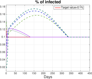
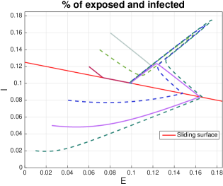
Figure 1: Motivating example: epidemic control The theory developed in this paper proves the convergence of sliding-mode controllers applied to a wide class of models. An example is the control of epidemic evolution as described e.g. by means of the SEIR model reported in (1). The target is to control the number of infected maintaining it to the desired value $I_{0}$. This can be done by influencing the time-course of the contact rate $\beta(t)$ through interventional measures that limit social interaction. As discussed later on, in this case a convenient sliding-mode surface is defined by $\epsilon E-\delta I+\lambda(I-I_{0})=0$ where $\lambda>0$ and the (discontinuous) feedback law sets a lockdown if $\lambda(I-I_{0})+\dot{I}>0$. For simplicity, we can now think that two values for the contact rate $\beta(t)$ are alternated, equal to $\beta_{F}$ when no restrictions are set and to $\beta_{L}$ during the lockdown. The theory developed in this paper provides the necessary and sufficient conditions ensuring that, for any system initial condition, the equilibrium point is reached and maintained (until the epidemic dies out). Some time-courses of the number of infected generated by the closed-loop system are shown in the left panel. They all converge to the target value $I_{0}$ that is set to $0.1\%$ of the population (horizontal line). The right panel also displays the corresponding trajectories over the exposed-infected plane and the sliding region (red straight line). Adopted parameter values are $\beta_{F}=0.8$, $\beta_{L}=0.2$ (associated trajectories are plotted using solid lines) or $0.21$ (dashed lines), $\delta=\epsilon=0.2$, $\lambda=1$. Attractiveness of the sliding region visible in figure is the manifestation of the general sliding-mode convergence theory under feedback constraints developed in the paper. Examples treated in what follows will regard also other epidemiological models, like SAIR and SEAIR, that incorporate the class of asymptomatic people who are known to play a major role in transmitting COVID-19.

III Results

III-A Sliding-mode convergence theorem under feedback contraints

The following theorem represents the main result of this paper. It considers a state-space $n$-dimensional linear model whose input is defined by a state feedback subject to a time-varying gain $\gamma(t)$. Such gain is uniformly bounded in time, a constraint defined by the union of two disjoint sets $I_{1}$ and $I_{2}$. The control target is to make systems dynamics follow the Hurwitz polynomial $\Delta(s)$ of degree $n-1$. The necessary and sufficient conditions for a sliding-mode controller to satisfy such requirement are then obtained (the proof is reported in Appendix).

Theorem 1

Consider the following single-input linear system with $\dim(x)=n$

$$\dot{x}=Fx+gu,\ u=Hx\gamma(t),$$

where $\gamma(t)$ is a bounded time-varying gain. We are also given a pair of disjoint intervals $I_{1}=[\gamma_{1}^{(1)},\gamma_{1}^{(2)}],I_{2}=[\gamma_{2}^{(1)},\gamma_{2}^{(2)}]$, with $\gamma_{1}^{(2)}<\gamma_{2}^{(1)}$, such that $\gamma(t)\in I_{1}\cup I_{2}$ for any $t\geq 0$, and an arbirary $(n-1)-$degree Hurwitz polynomial $\Delta(s)=s^{n-1}+\dots+\Delta_{1}s+\Delta_{0}$.

Then

there exist a unique matrix $K$, a unique $\gamma_{0}\in[\gamma_{1}^{(2)},\gamma_{2}^{(1)}]$ and a point $x_{eq}\neq 0$ (univocally defined except for a multiplicative constant) such that

• $[F+gH\gamma_{0}]x_{eq}=0$;

• the following control law

  $$\begin{array}[]{lcl}\gamma(t)&=&\ \mbox{any value}\ \in I_{1}\ \ \mbox{if}\ \ (Hx_{eq})[K(x-x_{eq})]<0,\cr\gamma(t)&=&\ \mbox{any value}\ \in I_{2}\ \ \mbox{if}\ \ (Hx_{eq})[K(x-x_{eq})]>0\end{array}$$

  leads to the sliding surface $Kx=Kx_{eq}$, endowed with dynamics associated to the characteristic polynomial $\Delta(s)$;

• the sliding surface is (at least) locally attractive in a suitable open neighborhood ${\mathcal{I}}$ of $x_{eq}$. Hence,

  • ${\mathcal{I}}$ is invariant, i.e. $x(0)\in{\mathcal{I}}$ implies $x(t)\in{\mathcal{I}}$, for any $t\geq 0$;

  • $x(0)\in{\mathcal{I}}$ implies that $x(t)$ reaches the sliding surface in finite time. From that time onwards $x(t)$ does not escape from it and then $x(t)$ tends to $x_{eq}$ for $t$ tending to $+\infty$,

if and only if

the following conditions hold true

• $(F,g)$ is a controllable pair;

• $\det[F+gH\gamma_{1}^{(2)}]\det[F+gH\gamma_{2}^{(1)}]<0$.

III-B Applications to epidemic control

As already anticipated, despite the apparent linear assumptions, the applicability of the theorem extends well beyond this setting. To this regard, the time-varying gain $\gamma(t)$ plays a crucial role since it can be used to capture also hidden nonlinear parts of a system. This fact will become clear through the following illustrations regarding epidemic control. We start treating the SEIR model that was the basis of our motivating example.

III-B1 SEIR

Consider now (1), define

$$\gamma(t):=\beta(t)S(t)$$

and let $I_{0}$ be the desired number of infected at the equilibrium. The equations describing the interactions between removed and susceptible are not important now, one has just to take into account that $S(t)$ decreases in time. Then, we can write

$$\dot{E}=\gamma(t)I-\epsilon E,\ \dot{I}=\epsilon E-\delta I$$

that implies

$$\begin{bmatrix}\dot{E}\cr\dot{I}\end{bmatrix}=\begin{bmatrix}-\epsilon&0\cr\epsilon&-\delta\end{bmatrix}\begin{bmatrix}E\cr I\end{bmatrix}+\begin{bmatrix}1\cr 0\end{bmatrix}\begin{bmatrix}0&1\end{bmatrix}\begin{bmatrix}E\cr I\end{bmatrix}\gamma(t).$$

This leads to the following correspondences with the matrices and the equilibrium point entering Theorem 1

$$F=\begin{bmatrix}-\epsilon&0\cr\epsilon&-\delta\end{bmatrix},\ g=\begin{bmatrix}1\cr 0\end{bmatrix},\ H=\begin{bmatrix}0&1\end{bmatrix},\ x_{eq}=\begin{bmatrix}\frac{\delta}{\epsilon}\cr 1\end{bmatrix}I_{0},\ I_{0}>0,$$

where the polynomial defining the desired system dynamics is given by $\Delta(s)=s+\lambda$ with $\lambda>0$. We can alternate lockdown and freedom periods where, for simplicity, we assume that the contact rate is equal to $\beta_{L}$ and $\beta_{F}$, respectively. It is easy to see that the couple $(F,g)$ is controllable while the condition on the product of the determinants becomes

$$\det[F+gH\gamma_{1}^{(2)}]\det[F+gH\gamma_{2}^{(1)}]=\epsilon^{2}\big{(}\delta-\gamma_{1}^{(2)}\big{)}\big{(}\delta-\gamma_{2}^{(1)}\big{)}<0.$$

This latter permits to conclude that sliding-mode SEIR control works properly as long as

$$\gamma_{1}(t):=\beta_{L}S(t)<\delta<\beta_{F}S(t):=\gamma_{2}(t).$$ (2)

Since $Hx_{eq}=I_{0}>0$, from Theorem 1 one also obtains that the lockdown has to be introduced when $K(x-x_{eq})<0$. Here, exploiting the arguments of the theorem’s proof contained in Appendix, the matrix $K$ is calculated using the controllability matrices ${\mathcal{R}}$ and ${\mathcal{R}}_{c}$ of the original system and of that in controllability canonical form [15], respectively. In particular, to obtain $\Delta(s)=s+\lambda$ one has

$$K_{c}=\begin{bmatrix}-\lambda&-1\end{bmatrix}\ \Rightarrow\ K=K_{c}{\mathcal{R}}_{c}{\mathcal{R}}^{-1}=\begin{bmatrix}-1&\frac{\delta-\lambda}{\epsilon}\end{bmatrix}.$$

Hence, one obtains

$$\mbox{Lockdown}\ \Leftrightarrow\ \begin{bmatrix}-1&\frac{\delta-\lambda}{\epsilon}\end{bmatrix}\begin{bmatrix}E-E_{0}\cr I-I_{0}\end{bmatrix}<0,$$

a condition that, using $E_{0}=\frac{\delta}{\epsilon}I_{0}$, can be rewritten as

$$\mbox{Lockdown}\ \Leftrightarrow\ \epsilon E-\delta I+\lambda(I-I_{0})>0\ \ \Leftrightarrow\ \lambda(I-I_{0})+\dot{I}>0.$$

We have so found the form of the sliding-mode controller anticipated in the description of Fig. 1 that, remarkably, is completely independent of the system parameters.
As said, the sliding surface will be reached and maintained only if (2) holds true. We can now reconsider the numerical experiments in Fig. 1, where any state trajectory is generated using the SEIR with $\delta=0.2$. When $\beta_{L}=0.2$, the condition in (2) is satisfied since $S(0)<1$. This explains why all the associated trajectories (solid lines) quickly converge to the sliding surface.
The two situations where (2) is not satisfied are

• $\beta_{L}S(t)>\delta$. In fact, one system eigenvalue is positive and the other one negative both during the lockdown and in absence of restrictions. Hence, the epidemic grows independently of any control action (even during the lockdown) until $S(t)$ becomes sufficiently small to satisfy the condition in (2). This is exactly what happens in Fig. 1 when $\beta_{L}=0.21$ is adopted. Only when $S(t)$ decreases enough the associated trajectories (dashed lines) are attracted by the sliding line;

• $\beta_{F}S(t)<\delta$. The two system eigenvalues are now real and negative both during the lockdown and the freedom period. The sliding surface can not be reached and maintained because the epidemic dies down on its own, independently of any action.

Note also that, when (2) is satisfied, the feedback law makes the equilibrium point $I_{0}>0$ asymptotically stable but then, when $S(t)$ becomes small enough, the second case described above will take place. The system will leave the sliding surface and the epidemic will end without the need of any restriction.
As a final but important note, Theorem 1 provides the necessary and sufficient conditions for asymptotic stability without specifying the domain of attraction ${\mathcal{I}}$ around the equilibrium point $x_{eq}$. This will depend on the particular system under study. Remarkably, in the SEIR case also global convergence holds, i.e. convergence is ensured for any non null system initial condition if (2) is fullfilled. The proof of this result is somewhat technical and can be found in Appendix, see section V-B.

III-B2 SAIR

Using the SAIR, infected are divided into two classes, denoted by $A$ and $I$. Class $A(t)$ contains asymptomatic or paucisymptomatic who can either directly recover with a rate established by $\epsilon_{2}$ or move to the second class $I(t)$ with a rate $\epsilon_{1}$. From $I(t)$, they can then recover with a rate $\delta$. Dynamics are thus given by

$$\dot{S}(t) =-\beta(t)S(t)\big{(}A(t)+I(t)\big{)}$$ (3a)

$$\dot{A}(t) =\beta(t)S(t)\big{(}A(t)+I(t)\big{)}-\big{(}\epsilon_{1}+\epsilon_{2}\big{)}A(t)$$ (3b)

$$\dot{I}(t) =\epsilon_{1}A(t)-\delta I(t)$$ (3c)

$$\dot{R}(t) =\epsilon_{2}A(t)+\delta I(t).$$ (3d)

The infection rate $\beta(t)$ now describes how the interaction between susceptible $S(t)$ and the two classes $A(t),I(t)$ of infected evolves in time.
To exploit Theorem 1, by adopting arguments very similar to those introduced in the SEIR case, the following matrices and equilibrium point are derived

$$F=\begin{bmatrix}-(\epsilon_{1}+\epsilon_{2})&0\cr\epsilon_{1}&-\delta\end{bmatrix},\ g=\begin{bmatrix}1\cr 0\end{bmatrix},$$

$$H=\begin{bmatrix}1&1\end{bmatrix},\ x_{eq}=\begin{bmatrix}\frac{\delta}{\epsilon_{1}}\cr 1\end{bmatrix}I_{0},\ I_{0}>0.$$

As done before, the contact rate may switch between the levels $\beta_{L}$ and $\beta_{F}$ during the lockdown and the freedom period, respectively. Also in this case the couple $(F,g)$ is controllable while the condition on the determinants becomes

$$\det[F+gH\gamma_{1}^{(2)}]\det[F+gH\gamma_{2}^{(1)}]$$

$$=\big{(}\delta(\epsilon_{1}+\epsilon_{2})-\gamma_{1}^{(2)}(\delta+\epsilon_{1})\big{)}\big{(}\delta(\epsilon_{1}+\epsilon_{2})-\gamma_{2}^{(1)}(\delta+\epsilon_{1})\big{)}<0.$$

Hence, the key condition for effectiveness of sliding-mode SAIR control is

$$\gamma_{1}(t):=\beta_{L}S(t)<\frac{\delta(\epsilon_{1}+\epsilon_{2})}{\delta+\epsilon_{1}}<\beta_{F}S(t):=\gamma_{2}(t).$$ (4)

One can thus see how the dynamics of asymptomatic people influence the control threshold through the parameters $\epsilon_{1},\epsilon_{2}$. The desired system dynamics are still defined by $\Delta(s)=s+\lambda$ with $\lambda>0$. So, one has $K_{c}=\begin{bmatrix}-\lambda&-1\end{bmatrix}$ and using again $K=K_{c}{\mathcal{R}}_{c}{\mathcal{R}}^{-1}$, simple calculations lead to

$$K=\begin{bmatrix}-1&\frac{\delta-\lambda}{\epsilon_{1}}\end{bmatrix}.$$

This implies the following control law

$$\mbox{Lockdown}\ \Leftrightarrow\ \lambda(I-I_{0})+\dot{I}>0$$

that coincides with that achieved in the SEIR case. It is also easy to see that the sliding surface now satisfies the equation

$$\epsilon_{1}A+(\lambda-\gamma)I=I_{0}\lambda.$$

Remarkably, even in the SAIR case global convergence holds, see section V-B in Appendix.

III-B3 SEAIR

The SEAIR model is a generalization of the SEIR and SAIR that embeds both the exposed and the asymptomatic class. It is given by

$$\dot{S} =-\beta(t)S(t)(A+I)$$ (5a)

$$\dot{E} =\beta(t)S(t)(A+I)-\epsilon E$$ (5b)

$$\dot{A} =\epsilon E-(\epsilon_{1}+\epsilon_{2})A$$ (5c)

$$\dot{I} =\epsilon_{1}A-\delta I$$ (5d)

$$\dot{R} =\epsilon_{2}A+\delta I.$$ (5e)

Using the same arguments introduced for the analysis of the SEIR and SAIR, we can focus on the variables $(E,A,I)$ and use $\gamma(t)$ to account for the other hidden nonlinear dynamics. One obtains the matrices

$$F=\begin{bmatrix}-\epsilon&0&0\cr\epsilon&-(\epsilon_{1}+\epsilon_{2})&0\cr 0&\epsilon_{1}&-\delta\end{bmatrix},\ g=\begin{bmatrix}1\cr 0\cr 0\end{bmatrix},$$

$$H=\begin{bmatrix}0&1&1\end{bmatrix},\ x_{eq}=\begin{bmatrix}\frac{\delta(\epsilon_{1}+\epsilon_{2})}{\epsilon\epsilon_{1}}\cr\frac{\delta}{\epsilon_{1}}\cr 1\end{bmatrix}I_{0},\ I_{0}>0.$$

We still assume that the contact rate can switch only between $\beta_{L}$ and $\beta_{F}$ alternating lockdown and freedom periods, respectively. Similarly to the other cases, the couple $(F,g)$ is controllable while one now has

$$\det[F+gH\gamma_{1}^{(2)}]\det[F+gH\gamma_{2}^{(1)}]$$

$$=\epsilon^{2}\big{(}\delta(\epsilon_{1}+\epsilon_{2})-\gamma_{1}^{(2)}(\delta+\epsilon_{1})\big{)}\big{(}\delta(\epsilon_{1}+\epsilon_{2})-\gamma_{2}^{(1)}(\delta+\epsilon_{1})\big{)}<0.$$

Thus, sliding-mode SEAIR control requires fulfilment of the same condition related to the SAIR and reported in (4), i.e. once again one needs

$$\gamma_{1}(t):=\beta_{L}S(t)<\frac{\delta(\epsilon_{1}+\epsilon_{2})}{\delta+\epsilon_{1}}<\beta_{F}S(t):=\gamma_{2}(t).$$ (6)

Let now the Hurwitz polynomial be $\Delta(s)=s^{2}+\Delta_{1}s+\Delta_{0}$. To derive the sliding-mode control form, calculations are more difficult than in the previous cases so, to make the exposition more compact, we think backwards verifying that

$$\mbox{Lockdown}\ \Leftrightarrow\ddot{I}+\Delta_{1}\dot{I}+\Delta_{0}(I-I_{0})>0.$$ (7)

In fact, in view of the definition of $\Delta(s)$, one now has

$$K_{c}=\begin{bmatrix}-\Delta_{0}&-\Delta_{1}&-1\end{bmatrix}.$$ (8)

In addition,

$$\dot{I}=\epsilon_{1}A-\delta I\ \Rightarrow\ \ddot{I}=\epsilon_{1}\dot{A}-\delta\dot{I}=\epsilon_{1}[\epsilon E-(\epsilon_{1}+\epsilon_{2})A]-\delta[\epsilon_{1}A-\delta I]$$

that implies

$$\ddot{I}+\Delta_{1}\dot{I}+\Delta(I-I_{0})=\epsilon_{1}\dot{A}-\delta\dot{I}$$

$$=\epsilon_{1}[\epsilon E-(\epsilon_{1}+\epsilon_{2})A]-\delta[\epsilon_{1}A-\delta I]+\Delta_{1}[\epsilon_{1}A-\delta I]+\Delta_{0}(I-I_{0}).$$

This means that the lockdown’s condition $\ddot{I}+\Delta_{1}\dot{I}+\Delta_{0}(I-I_{0})>0$ can be rewritten as

$$\epsilon\epsilon_{1}E-\epsilon_{1}(\epsilon_{1}+\epsilon_{2}+\delta-\Delta_{1})A+(\delta^{2}-\delta\Delta_{1}+\Delta_{0})I-\Delta_{0}I_{0}>0.$$

Letting

$$K:=h\begin{bmatrix}-\epsilon\epsilon_{1}&\epsilon_{1}(\epsilon_{1}+\epsilon_{2}+\delta-\Delta_{1})&-(\delta^{2}-\delta\Delta_{1}+\Delta_{0})\end{bmatrix},$$ (9)

with $h$ being any positive scale factor, the previous condition becomes

$$-Kx-h\Delta_{0}I>0\ \Rightarrow\ Kx+h\Delta_{0}I_{0}<0\ \Rightarrow\ K(x-x_{eq})<0$$

(since $Kx_{eq}=-h\Delta_{0}I_{0}$). To derive $h$, we know that the relationship $K{\mathcal{R}}=K_{c}{\mathcal{R}}_{c}$ must hold where, in the SEAIR case, the controllability matrices are

$${\mathcal{R}}=\begin{bmatrix}1&-\epsilon&\epsilon^{2}\cr 0&\epsilon&-\epsilon(\epsilon+\epsilon_{1}+\epsilon_{2})\cr 0&0&\epsilon\epsilon_{1}\end{bmatrix},$$

$$\tiny{\mathcal{R}}_{c}=\begin{bmatrix}0&0&1\cr 0&1&-(\delta+\epsilon+\epsilon_{1}+\epsilon_{2})\cr 1&-(\delta+\epsilon+\epsilon_{1}+\epsilon_{2})&-\epsilon\delta-(\epsilon+\delta)(\epsilon_{1}+\epsilon_{2})+(\delta+\epsilon+\epsilon_{1}+\epsilon_{2})^{2}\end{bmatrix}.$$

Recalling (8) and (9), it becomes easy to conclude that $h=\frac{1}{\epsilon\epsilon_{1}}$ is necessary and also sufficient for $K{\mathcal{R}}=K_{c}{\mathcal{R}}_{c}$ to hold. Thus,

$$K=\begin{bmatrix}-1&\frac{\epsilon_{1}+\epsilon_{2}+\delta-\Delta_{1}}{\epsilon}&-\frac{\delta^{2}-\delta\Delta_{1}+\Delta_{0}}{\epsilon\epsilon_{1}}\end{bmatrix}$$

is the unique $K$ obtainable from Theorem 1, hence proving the correctness of the postulated feedback law in (7) that, as in the previous cases, does not depend on system parameters.

IV Conclusions

The convergence of sliding-mode controllers subject to strong structural constraints on the feedback law has been investigated in this paper. The fundamental assumption that permeates this work is that the control input may assume values only over two bounded and disjoint sets that could be also non perfectly known. The necessary and sufficient conditions for an effective control of a class of time-varying continuous-time linear systems, that includes all the time-invariant linear state-space models, have been obtained. A rather general family of controllers is so derived which guarantees to reach the sliding surface and maintain the desired equilibrium point. Notably, the analysis is only apparently restricted to the linear setting since the class of dynamic systems here introduced is wider than expected. In fact, the cases reported in the previous section illustrate how the time-varying component present in our model can be conveniently used to describe hidden nonlinear dynamics. This permits to gain fundamental insights also on control of a wide class of nonlinear systems, making our findings relevant for the most varied applications. We have provided examples that regard well known epidemiological models that incorporate the classes of exposed and asymptomatic people, especially important e.g. to describe COVID-19 dynamics. Many previous works on epidemic control can thus be interpreted from a broader perspective, becoming special cases of the sliding-mode theory under feedback constraints here developed.
By exploiting the time-varying component that is integrated in the class of dynamic systems here proposed, SEIR and SAIR reduce to two-dimensional models. The fact that global convergence of sliding-mode controllers can be proved for these two systems leads also to an interesting open problem. In particular, we conjecture that global convergence holds for any positive and controllable two-dimensional system and we plan to investigate such issue in the next future.

V Appendix

V-A Proof of Theorem 1

A simple preliminary lemma is first obtained.

Lemma 2

Given

$$\dot{x}=Fx+gu,\ F\ \mbox{asymptotically stable},\ u(t)\ \mbox{bounded},\ u_{M}:=\sup_{t}\ |u(t)|$$

there exist a real number $a>0$ independent of $u_{M}$ and an open neighborhood ${\mathcal{I}}$ of $x=0$ such that

• ${\mathcal{I}}$ is an invariant set, i.e. $x(0)\in{\mathcal{I}}$ implies $x(t)\in{\mathcal{I}}$ for any $t\geq 0$;

• $\|{\mathcal{I}}\|:=sup_{x\in{\mathcal{I}}}\ \|x\|=au_{M}$.

Proof.  Let $P=P^{T}>0$ be the (unique) solution of the Lyapunov equation $F^{T}P+PF=-I$, and define

$${\mathcal{I}}(b):=\left\{\ x\in{\mathbb{R}}^{n}:\ x^{T}Px<b\ \right\},\ b>0\ \Rightarrow\ \|{\mathcal{I}}(b)\|=\sqrt{\frac{b}{\lambda_{MIN}(P)}}$$

Exploiting

$$\frac{d}{dt}x^{T}(t)Px(t)=\dot{x}^{T}Px+x^{T}P\dot{x}$$

$$=[Fx+gu]^{T}Px+x^{T}P[Fx+gu]=x^{T}(F^{T}P+PF)x+2x^{T}Pgu=$$

$$=-\|x(t)\|^{2}+2\|x(t)\|\frac{x^{T}(t)}{\|x(t)\|}Pgu(t)$$

$$\leq-\|x(t)\|^{2}+2\|x(t)\|u_{M}\max_{v:\ \|v\|=1}\ v^{T}Pg=$$

$$=-\|x(t)\|\Big{(}\|x(t)\|-2u_{M}\max_{v:\ \|v\|=1}\ v^{T}Pg\Big{)}$$

and

$$\|x(t)\|\geq\sqrt{\frac{x^{T}(t)Px(t)}{\lambda_{MAX}(P)}}$$

it follows that

$$x^{T}(t)Px(t)>4\lambda_{MAX}(P)u_{M}^{2}\Big{(}\max_{v:\ \|v\|=1}\ v^{T}Pg\Big{)}^{2}$$

implies

$$\frac{d}{dt}x^{T}(t)Px(t)<0.$$

Let $b>0$ satisfy

$$b>4\lambda_{MAX}(P)u_{M}^{2}\Big{(}\max_{v:\ \|v\|=1}\ v^{T}Pg\Big{)}^{2}.$$

For a suitable $\mu>1$, one then has

$$\|{\mathcal{I}}(b)\|=2\mu\Big{(}\max_{v:\ \|v\|=1}\ v^{T}Pg\Big{)}\sqrt{\frac{\lambda_{MAX}(P)}{\lambda_{MIN}(P)}}u_{M}:=au_{M},$$

with

$$a:=2\mu\Big{(}\max_{v:\ \|v\|=1}\ v^{T}Pg\Big{)}\sqrt{\frac{\lambda_{MAX}(P)}{\lambda_{MIN}(P)}}.$$

Now, we want to show that ${\mathcal{I}}={\mathcal{I}}(b)$ satisfies the theorem statement by proving its invariance. In fact, assuming $x^{T}(0)Px(0)<b$, it holds that $x^{T}(t)Px(t)<b$ for any $t\geq 0$, otherwise a time instant $T>0$ would exist such that $x^{T}(T)Px(T)\geq b$. Because of the trajectory continuity, the set ${\mathcal{Z}}:=\{\ t\geq 0:\ x^{T}(t)Px(t)=b\ \}$ would be non-empty. Also, it would be equipped with an inferior $\bar{t}:=inf{\mathcal{Z}}$ which would imply $x^{T}(t)Px(t)<b$ for any $0<t<\bar{t}$, while $x^{T}(\bar{t})Px(\bar{t})=b$. One would thus obtain that $\frac{d}{dt}x^{T}(t)Px(t)$ would be strictly less than zero in a left neighborhood of $\bar{t}$, hence making $x^{T}(t)Px(t)>x^{T}(\bar{t})Px(\bar{t})$ for some $t<\bar{t}$. This contradicts the inferior property of $\bar{t}$. So, it must hold that ${\mathcal{Z}}=\emptyset$, from which $x^{T}(t)Px(t)<b$ for any $t\geq 0$ that is equivalent to the invariance property.

$\Box$

We are now in a position to prove the theorem. This will be done in five steps. The first four prove the sufficiency of the two conditions regarding controllability and the product of determinants while the last step discusses their necessity.

Step 1 [Existence of $x_{eq},\gamma_{0}$ and equations in terms of $x-x_{eq}$]
Let

$$\Delta_{F}(s)=s^{n}+\dots+a_{1}s+a_{0}$$

be the characteristic polynomial of $F$. Consider the system in controllability canonical form (where also $H$ has been accordingly modified)

$$T^{-1}FT=F_{c},\ T^{-1}g=g_{c},\ H_{c}:=HT,$$

with $T={\mathcal{R}}{\mathcal{R}}_{c}^{-1}$ where ${\mathcal{R}}$ and ${\mathcal{R}}_{c}$ are the controllability matrices of the original system and of that in controllability canonical form [15], respectively. The structure of these matrices permits to easily verify that

$$\det[F_{c}+g_{c}H_{c}\gamma(t)]=(-1)^{n}[a_{0}-H_{c}e_{1}\gamma(t)].$$

So, the second assumption implies

$$[a_{0}-H_{c}e_{1}\gamma_{1}^{(2)}][a_{0}-H_{c}e_{1}\gamma_{2}^{(1)}]<0$$

which means that $a_{0}-H_{c}e_{1}\gamma$ is linear in $\gamma$ and assumes opposite signs at $\gamma_{1}^{(2)},\gamma_{2}^{(1)}$. This implies that there exists a unique value $\gamma_{0}$, necessarily falling in the interval $(\gamma_{1}^{(2)},\gamma_{2}^{(1)})$, such that

$$\det[F_{c}+g_{c}H_{c}\gamma_{0}]=0\ \Leftrightarrow\ \det[F+gH\gamma_{0}]=0.$$

Also, this shows that a point $x_{eq}\neq 0$ exists such that $[F+gH\gamma_{0}]x_{eq}=0$ (and one easily sees that $\mbox{rank}[F_{c}+g_{c}H_{c}\gamma_{0}]=n-1$, so that $x_{eq}$ is uniquely determined except for a multiplicative constant), which implies $Fx_{eq}=-gH\gamma_{0}x_{eq}$. Hence

$$\dot{x}=F(x-x_{eq})+Fx_{eq}+gu=F(x-x_{eq})+g[u-H\gamma_{0}x_{eq}]$$

and, after defining $y:=x-x_{eq}$ and $v:=u-H\gamma_{0}x_{eq}$, one has

$$\dot{y}=Fy+gv$$

Step 2 [Construction of the sliding surface and related equations]
Consider again the controllability canonical form

$$\dot{z}=F_{c}z+g_{c}v,\ z:=T^{-1}y=\begin{bmatrix}\bar{z}\cr z_{n}\end{bmatrix}$$

where the last entry of $z$ has been highlighted. Consider any matrix $K_{c}:=\begin{bmatrix}k_{1}&k_{2}&\dots&k_{n-1}&-1\end{bmatrix}:=\begin{bmatrix}\bar{K}&-1\end{bmatrix}$ such that $\Delta(s):=s^{n-1}-k_{n-1}s^{n-2}+\dots-k_{2}s-k_{1}$ is an Hurwitz polynomial. Then, define $K$ through $K=K_{c}T^{-1}$, the sliding surface as $Kx=Kx_{eq}$, and the following change of variables

$$z=\begin{bmatrix}\bar{z}\cr z_{n}\end{bmatrix}=\begin{bmatrix}I&0\cr\bar{K}&-1\end{bmatrix}\begin{bmatrix}\bar{z}\cr K_{c}z\end{bmatrix}:=U\begin{bmatrix}\bar{z}\cr K_{c}z\end{bmatrix},\ U^{-1}=U,\ w:=\begin{bmatrix}\bar{z}\cr K_{c}z.\end{bmatrix}$$

First, notice that

$$\dot{z}=F_{c}z+g_{c}v\ \Rightarrow\ K_{c}\dot{z}=K_{c}F_{c}z+K_{c}g_{c}v=K_{c}F_{c}z-v$$

$$\Rightarrow\ K_{c}\dot{z}=r:=K_{c}F_{c}z-v\ \Rightarrow\ v=K_{c}F_{c}z-r$$

so that we can express the differential equations in terms of the new input $r$ as follows

$$\dot{z}=F_{c}z+g_{c}K_{c}F_{c}z-g_{c}r=(I+g_{c}K_{c})F_{c}z-g_{c}r.$$

This implies

$$\dot{w}=U(I+g_{c}K_{c})F_{c}Uw-Ug_{c}r=\begin{bmatrix}M&-\bar{g}_{c}\cr 0&0\end{bmatrix}w+\begin{bmatrix}0\cr 1\end{bmatrix}r$$

where $M$ is in companion form with the last row equal to $\bar{K}$, so that $\Delta_{M}(s)=\Delta(s)$ and $\bar{g}_{c}$ is like $g_{c}$ in $(n-1)$ dimensions. Also, by recalling the definition of $w$ and the relationships between $u,v,r$, it follows that

$$\dot{\bar{z}} = M\bar{z}-\bar{g}_{c}(K_{c}z)$$ (10)

$$(K_{c}\dot{z}) = r=K_{c}F_{c}z+Hx_{eq}\gamma_{0}-u$$ (11)

Step 3 [Condition for sliding activation]
By exploiting the second part of (11) one obtains

$$K_{c}\dot{z}=K_{c}F_{c}z+Hx_{eq}\gamma_{0}-u=K_{c}F_{c}z+Hx_{eq}\gamma_{0}-Hx\gamma(t)$$

$$=K_{c}F_{c}z+Hx_{eq}\gamma_{0}-Hy\gamma(t)-Hx_{eq}\gamma(t)=$$

$$=[K_{c}F_{c}-H_{c}\gamma(t)]z+Hx_{eq}[\gamma_{0}-\gamma(t)]$$

where $Hx_{eq}\neq 0$. Otherwise $(F+gH\gamma_{0})x_{eq}=0$ would imply $Fx_{eq}=0$ and also $(F+gH\gamma_{1}^{(2)})x_{eq}=0$, which would contradict the invertibility of the last matrix (recall that $x_{eq}\neq 0$). Since $K_{c}z=KTz=Ky=K(x-x_{eq})$, it follows that

$$K\dot{x}=[KF-H\gamma(t)](x-x_{eq})+Hx_{eq}[\gamma_{0}-\gamma(t)]$$

and, by defining

$$m:=\min\big{(}|Hx_{eq}(\gamma_{0}-\gamma_{1}^{(2)})|,|Hx_{eq}(\gamma_{0}-\gamma_{2}^{(1)})|\big{)}$$

and resorting to the control law described in the theorem statement, in case of

$$|[KF-H\gamma(t)](x-x_{eq})|<m-c,\ m>c>0$$ (12)

it holds that

$$|K\dot{x}|<c\ \ \mbox{and}\ \ \mbox{sign}[K\dot{x}]\mbox{sign}[K(x-x_{eq})]<0.$$

This implies that $K[x(t)-x_{eq}]=0$ from some $t<\frac{K[x(0)-x_{eq}]}{c}$ onwards, if (12) is satisfied by $x(t)$ for all $t\geq 0$, so establishing the sliding phenomenon in the surface $Kx=Kx_{eq}$. This fact is surely verified if

$$\|x(t)-x_{eq}\|<\frac{m-c}{\mu},\ \forall t\geq 0,$$

with

$$\mu:=\max_{(v,\gamma):\ \|v\|=1,\gamma_{1}\in I_{1},\gamma_{2}\in I_{2}}\ \{\ |[KF-H\gamma_{1}]v|,\ |[KF-H\gamma_{2}]v|\ \}.$$

Moreover, recalling that $w=Uz$ and $z=T^{-1}(x-x_{eq})$, the previous condition can be rewritten as

$$\|w(t)\|\leq b\|x(t)-x_{eq}\|<\frac{m-c}{b\mu}:=A,\ \forall t\geq 0,\ \mbox{for some $b>0$}.$$

This means that there exists a suitable $A>0$ such that

$$\|w(t)\|<A,\ \forall t\geq 0$$ (13)

and this implies that

$$\exists\ \bar{t}>0:\ |K[x(t)-x_{eq}]|\ \mbox{is monotone decreasing}$$

and

$$K[x(t)-x_{eq}]=0,\ \forall t\geq\bar{t},$$

so leading to the sliding establishment.

Step 4 [The invariant neighborhood of $x_{eq}$]
By applying Lemma 2 to the first part of (11), rewritten as

$$\dot{\bar{w}}=M\bar{w}-\bar{g}_{c}w_{n},\ w:=\begin{bmatrix}\bar{w}^{T}&w_{n}\end{bmatrix}^{T},$$

assuming that $w_{n}$ evolves in $\left(-d,d\right)$ implies the existence of an open neighborhood ${\mathcal{I}}_{\bar{w}}$ of $\bar{w}=0$ which is invariant. Moreover, for some $a>0$ one has

$$\|\bar{w}(t)\|<ad,\ \forall t\geq 0.$$

It follows that we can build the open neighborhood ${\mathcal{I}}_{w}:={\mathcal{I}}_{\bar{w}}\times\left(-d,d\right)$ of $w=0$ which is invariant and such that

$$\|w(t)\|=\sqrt{\|\bar{w}(t)\|^{2}+w_{n}^{2}}<d\sqrt{a^{2}+1}<A,\ \forall t\geq 0$$

if $d$ satisfies

$$0<d<\frac{A}{\sqrt{a^{2}+1}}.$$

Indeed, recalling also (11), this choice of $d$ ensures that $w_{n}$ evolves in $\left(-d,d\right)$, which is exactly what was required for guaranteeing both the invariance of ${\mathcal{I}}_{w}$ and the convergence to zero of $w_{n}(t)=K[x(t)-x_{eq}]$. Once the surface $w_{n}=0$ is reached, system dynamics on the sliding surface are simply given by $\dot{\bar{w}}=M\bar{w}$. This leads to a trajectory contained in ${\mathcal{I}}_{\bar{w}}$ (the input is now zero) in $(n-1)$ dimensions and in ${\mathcal{I}}_{\bar{w}}\times\{\ 0\ \}$ (which is a subset of ${\mathcal{I}}_{w}$) in $n$ dimensions. Hence, the invariance is maintained also after reaching the sliding surface and $w$ tends to zero without exiting from both $w_{n}=0$ and ${\mathcal{I}}_{w}$. As far as $x(t)-x_{eq}$ is concerned, the linear relationship between it and $w$ leads to a corresponding open neighborhood ${\mathcal{I}}$ of $x_{eq}$ that enjoys all the properties required in the theorem statement.

Step 5 [Necessity of the condition regarding controllability and negative sign of determinants product]
In the previous four steps, sufficiency of the sliding-mode control conditions regarding controllability and sign of the determinants product has been proved. We now demonstrate their necessity to conclude the theorem. If $(F,g)$ is not a controllable pair, any uncontrollable initial condition in $\mathcal{I}$ cannot be driven to any desired state, hence sliding-mode control could not work. The same conclusion can be obtained if the condition on the determinants is violated through the arguments developed in Step 1. In fact, one could not find any $\gamma_{0}\in(\gamma_{1}^{(2)},\gamma_{2}^{(1)})$ and corresponding $x_{eq}\neq 0$, as $\det[F+gH\gamma]$ linearly depends on $\gamma$.

V-B Global convergence of sliding-mode under feedback constraints for SEIR and SAIR

In the main part of this paper we have provided the necessary and sufficient conditions for asymptotic stability of a class of time-varying systems under sliding-mode control subject to feedback constraints. The theorem guarantees the existence of a domain of attraction ${\mathcal{I}}$ around the equilibrium point $x_{eq}$. The shape of ${\mathcal{I}}$ will depend on the particular system under study. As anticipated, in the SEIR and SAIR case global convergence holds, i.e. convergence is ensured with ${\mathcal{I}}$ set to the entire state space excluding the origin. The proof of this result is reported below. We just consider the SEIR case since the arguments concerning SAIR are completely analogous.

V-B1 Switching evolution

Let’s define the region ${\mathcal{R}}_{FREE}$ as the region where $\gamma(t)$ assumes the value $\gamma_{2}:=\gamma_{F}$

$${\mathcal{R}}_{FREE}:=\{\ (E,I)\geq 0:\ \epsilon E+(\lambda-\delta)I<\lambda I_{0}\ \}$$

and, analogously, the complementary region ${\mathcal{R}}_{LOCK}$ corresponding to $\gamma_{1}:=\gamma_{L}$. So, ${\mathcal{R}}_{FREE}\cup{\mathcal{R}}_{LOCK}\cup{\mathcal{L}}={\mathbb{R}}_{+}^{2}$, where ${\mathcal{L}}$ is the sliding line included in the positive quadrant. It is easy to see that a whole neighborhood of the origin is completely included in ${\mathcal{R}}_{FREE}$, and that ${\mathcal{L}}$ is either a segment or an half straight line (depending on the value of $\lambda>0$). Let’s introduce the Frobenius’s eigenvalue $\lambda_{FR}>0$ associated with the matrix $F_{FREE}:=F+gH\gamma_{F}$ and the corresponding positive eigenvector $w_{FR}$. Simple computations lead to

$$w_{FR}=2\begin{bmatrix}\lambda_{FR}+\delta&\epsilon\end{bmatrix}^{T}=\begin{bmatrix}(\delta-\epsilon)+\sqrt{(\delta-\epsilon)^{2}+4\epsilon\gamma_{F}}&2\epsilon\end{bmatrix}^{T},$$

$$\lambda_{FR}=\frac{-(\delta+\epsilon)+\sqrt{(\delta-\epsilon)^{2}+4\epsilon\gamma_{F}}}{2},$$

so that the intersection of ${\mathcal{L}}$ with the half straight line $x=aw_{FR},\ a\geq 0$ is easily found

$$(E,I)=\begin{pmatrix}\frac{\lambda(\delta+\lambda_{FR})}{\epsilon(\lambda+\lambda_{FR})}&\frac{\lambda}{\lambda+\lambda_{FR}}\end{pmatrix}I_{0}>0.$$

Since $\lambda,\lambda_{FR}>0$, the point $I_{FR}$ where the intersection takes place satisfies $0<I_{FR}<I_{0}$. This means that, regardless of the nature (finite or infinite) of ${\mathcal{L}}$, there always exists an intersection in the positive quadrant. But this implies that, starting from any $x(0)\in{\mathcal{R}}_{FREE},\ x(0)\neq 0$, at a certain instant $x(t)$ leaves ${\mathcal{R}}_{FREE}$ and touches the sliding line. This happens because, by using $w$ to denote the other eigenvector of $F_{FREE}$, $x(0)\geq 0,\ x(0)\neq 0$ implies $x(0)=aw_{FR}+bw$ (with $a>0$ in view of the positive systems properties), so that $x(t)$ tends to grow as $e^{\lambda_{FR}t}$ and to follow the direction of $w_{FR}$. Existence of the intersection at $I_{FR}$ also ensures the existence of a time instant $t>0$ such that $x(t)$ belongs to ${\mathcal{L}}$, hence leaving ${\mathcal{R}}_{FREE}$. Note that this is obvious in case of a finite sliding line, while in the infinite case the proof of existence of the aforementioned intersection is required. The same holds true for ${\mathcal{R}}_{LOCK}$ too. For any $x(0)\in{\mathcal{R}}_{LOCK}$, sooner or later ${\mathcal{L}}$ is reached again, in this case because of the asymptotic stability of $F+gH\gamma_{L}:=F_{LOCK}$ which makes $x(t)$ convergent to zero. So, it suffices to recall that a whole neighborhood of the origin is included in ${\mathcal{R}}_{FREE}$. This property of the sliding line allows us to study the sliding establishment by considering only initial conditions in ${\mathcal{L}}$.

V-B2 The sliding establishment zone

Define

$$I_{MAX}:=\frac{\lambda}{\lambda-\delta}I_{0}\ \mbox{(if $\lambda>\delta$)},\ I_{MAX}:=+\infty\ \mbox{(if $0<\lambda\leq\delta$)}$$

so that $I$, on the sliding line, can assume only values in $[0,I_{MAX}]$. Now we investigate the behavior of the sliding line points, by showing that only the following three cases may arise:

• the flow goes from ${\mathcal{R}}_{FREE}$ towards ${\mathcal{R}}_{LOCK}$;

• the flow goes from ${\mathcal{R}}_{LOCK}$ towards ${\mathcal{R}}_{FREE}$;

• the flow goes both from ${\mathcal{R}}_{FREE}$ towards ${\mathcal{R}}_{LOCK}$ and from ${\mathcal{R}}_{LOCK}$ towards ${\mathcal{R}}_{FREE}$.

In the first two cases, when considered as mutually exclusive, the trajectory crosses the sliding line. The third case corresponds to points belonging to the subset of ${\mathcal{L}}$ where the trajectory cannot escape from ${\mathcal{L}}$ itself, so establishing the sliding mode converging to $I_{0}$. It thus corresponds to the overlapping of the first two cases.

V-B3 Flow from ${\mathcal{R}}_{FREE}$ to ${\mathcal{R}}_{LOCK}$

We start by analyzing which points are related to the first situation. This requires to assume $K\dot{x}<0$, with $\dot{x}=F_{FREE}x$, together with $K(x-x_{eq})=0$. We easily obtain the following inequality

$$[\lambda^{2}-(\delta+\epsilon)\lambda-\epsilon(\gamma_{F}-\delta)]I<\lambda(\lambda-\epsilon-\delta)I_{0}$$

which, for suitable $\lambda_{1},\lambda_{2}>0$, can be rewritten as

$$(\lambda-\lambda_{1})(\lambda+\lambda_{2})I<\lambda(\lambda-\epsilon-\delta)I_{0},\ \lambda_{1}>\epsilon+\delta.$$

Obviously, both $I_{0}$ and $I_{FR}$ always satisfy the inequality. By defining

$$I_{1}:=\frac{\lambda(\lambda-\epsilon-\delta)}{\lambda^{2}-(\delta+\epsilon)\lambda-\epsilon(\gamma_{F}-\delta)}$$

the previous inequality becomes something like either $I>I_{1}$ or $I<I_{1}$, depending on the signs of the left and right side terms. One has also to take into account that $I$ cannot be either negative or exceed $I_{MAX}$. After discriminating among a certain number of cases, it follows that if $\lambda>\lambda_{1}$ the inequality’s solution is given by $I<I_{1}$, with $I_{1}>I_{0}>I_{FR}$. However, $I_{1}>I_{MAX}$ if $\lambda_{1}<\lambda<\delta+\frac{\epsilon}{\delta}\gamma_{FR}$, so that

• if $\lambda>\delta+\frac{\epsilon}{\delta}\gamma_{F}$, then $I<I_{1}$, with $I_{MAX}>I_{1}>I_{0}>I_{FR}>0$

• if $\lambda_{1}<\lambda\leq\delta+\frac{\epsilon}{\delta}\gamma_{F}$, then $I$ is any.

The second case is $\lambda_{1}\geq\lambda\geq\epsilon+\delta$, which leads again to $I$ being any, while the third case is $\epsilon+\delta>\lambda>0$, which leads to $I>I_{1}$, with $I_{MAX}>I_{0}>I_{FR}>I_{1}>0$. All of these outcomes are summarized below.

The flow goes from ${\mathcal{R}}_{FREE}$ to ${\mathcal{R}}_{LOCK}$

• if $\lambda>\delta+\frac{\epsilon}{\delta}\gamma_{F}$, then $I<I_{1}$, with $I_{MAX}>I_{1}>I_{0}>I_{FR}>0$;

• if $\delta+\epsilon\leq\lambda\leq\delta+\frac{\epsilon}{\delta}\gamma_{F}$, then $I$ is any;

• if $\epsilon+\delta>\lambda>0$, then $I>I_{1}$, with $I_{MAX}>I_{0}>I_{FR}>I_{1}>0$.

V-B4 Flow from ${\mathcal{R}}_{LOCK}$ to ${\mathcal{R}}_{FREE}$

Now we consider points related to the second situation. This requires to assume $K\dot{x}>0$, with $\dot{x}=F_{LOCK}x$, together with $K(x-x_{eq})=0$. The following inequality is easily obtained

$$[\lambda^{2}-(\delta+\epsilon)\lambda+\epsilon(\delta-\gamma_{L})]I>\lambda(\lambda-\epsilon-\delta)I_{0}.$$

For suitable $\lambda_{3},\lambda_{4}>0$ satisfying $0<\lambda_{4}<\delta<\lambda_{3}<\delta+\epsilon$, it can be rewritten as

$$(\lambda-\lambda_{3})(\lambda-\lambda_{4})I>\lambda(\lambda-\epsilon-\delta)I_{0}.$$

Again, $I_{0}$ always satisfies the inequality, and by defining

$$I_{2}:=\frac{\lambda(\lambda-\epsilon-\delta)}{\lambda^{2}-(\delta+\epsilon)\lambda+\epsilon(\delta-\gamma_{L})}$$

the previous inequality becomes something like either $I>I_{2}$ or $I<I_{2}$, depending on the signs of the left and right side terms. We have also to take into account that $I$ cannot be either negative or exceed $I_{MAX}$. It follows that if $\lambda>\delta+\epsilon$ the inequality solution is given by $I>I_{2}$, with $I_{MAX}>I_{0}>I_{2}>0$. If $\delta+\epsilon\geq\lambda\geq\lambda_{3}$ then $I$ can be any, while if $\delta<\lambda<\lambda_{3}$ it becomes $I<I_{2}$, with $I_{2}>I_{0}$. However, also in this case we have to verify whether $I_{2}<I_{MAX}$ and this actually holds only if $\delta<\lambda<\delta+\frac{\epsilon}{\delta}\gamma_{L}<\lambda_{3}$. Moreover, the same situation $I<I_{2}$, with $I_{MAX}>I_{2}>I_{0}$, occurs if $\delta\geq\lambda>\lambda_{4}$, while $I$ can assume any value if $0<\lambda<\lambda_{4}$. We summarize these outcomes below.

The flow goes from ${\mathcal{R}}_{LOCK}$ to ${\mathcal{R}}_{FREE}$

• if $\lambda>\delta+\epsilon$, then $I>I_{2}$, with $I_{MAX}>I_{0}>I_{2}>0$;

• if $\delta+\epsilon\geq\lambda\geq\delta+\frac{\epsilon}{\delta}\gamma_{L}$, then $I$ is any;

• if $\lambda_{4}<\lambda<\delta+\frac{\epsilon}{\delta}\gamma_{L}$, then $I<I_{2}$, with $I_{MAX}>I_{2}>I_{0}>0$;

• if $0<\lambda<\lambda_{4}$, then $I$ is any.

V-B5 The attractive sliding zone

Considering all the results obtained so far, we can notice that, whenever the whole ${\mathcal{L}}$ is attractive at least in one direction (which means that all the trajectories go either from ${\mathcal{R}}_{LOCK}$ towards ${\mathcal{R}}_{FREE}$ or conversely), the trajectory can cross ${\mathcal{L}}$ at most once before falling into the sliding establishment. Therefore, it holds that

• if $\lambda>\delta+\frac{\epsilon}{\delta}\gamma_{F}$, the trajectory leaves ${\mathcal{R}}_{FREE}$ for $I<I_{2}$ and then it comes back into ${\mathcal{R}}_{FREE}$ for $I>I_{1}$ (with $I_{1}>I_{2}$). This implies the possible existence of trajectories turning in counterclockwise direction without ever falling into the sliding zone $(I_{2},I_{1})$. From previous results, it easily holds that $I_{MAX}>I_{1}>I_{0}>I_{2}>I_{FR}>0$ where $I_{2}>I_{FR}$;

• if $\delta+\frac{\epsilon}{\delta}\gamma_{F}\geq\lambda\geq\delta+\frac{\epsilon}{\delta}\gamma_{L}$ the sliding zone is reached after at most one sliding line crossing;

• if $\delta+\frac{\epsilon}{\delta}\gamma_{L}>\lambda>\lambda_{4}$, the trajectory leaves ${\mathcal{R}}_{FREE}$ for $I>I_{2}$ and then it comes back into ${\mathcal{R}}_{FREE}$ for $I<I_{1}$ (with $I_{2}>I_{1}$). This implies the possible existence of trajectories turning in clockwise direction without ever falling into the sliding zone $(I_{1},I_{2})$ (this case includes situations in which the sliding line is either a segment or an half straight line). Previous results show that $I_{MAX}>I_{2}>I_{0}>I_{FR}>I_{1}>0$;

• if $0<\lambda<\lambda_{4}$ the sliding zone is reached after at most one sliding line crossing.

If $\delta+\frac{\epsilon}{\delta}\gamma_{L}>\lambda>\lambda_{4}$ the sliding zone is reached after crossing at most two times the sliding line, in view of the position of $I_{FR}$ (inside the sliding zone). In fact, assume (as worst case) that the trajectory starts in ${\mathcal{R}}_{FREE}$ and crosses the sliding line at some $I_{3}>I_{2}$, then coming back to ${\mathcal{R}}_{FREE}$ at some $I_{4}<I_{1}$ (another possibility would be that the trajectory directly falls into the sliding zone). Then, the trajectory cannot touch the line $aw_{FR},\ a\geq 0$, otherwise this would contradict the unicity of the differential equations solution. In fact, by contradiction, let $P$ be a point in which the latter line is touched. Then two solutions, starting one from the point corresponding to $I_{4}$ and the other from any point of the form $aP$ with $0<a<1$, would reach the same point $P$, and this is impossible (the solution is unique also by reverting the time direction). In other words, two different solutions cannot intersect, unless they are the same (periodic) one. So the trajectory coming from $I_{4}$ necessarily would fall on the sliding line into a point included in the interval $(I_{1},I_{FR})$, which is a subset of the sliding zone $(I_{1},I_{2})$, and no other crossings at some $I>I_{2}$ would be possible. This shows that the only case that needs to be further investigated is the first one, i.e. $\lambda>\delta+\frac{\epsilon}{\delta}\gamma_{F}$. In this case the position of $I_{FR}$ does not prevent multiple crossings of the sliding line, see also Fig. 2.

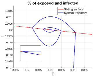
Figure 2: Multiple crossings example State trajectories on the $(E,I)-$plane with $\lambda=10,\delta=0.05,\epsilon=0.2,\gamma_{F}=0.065$ and $I_{0}=2\times 10^{-3}$. The condition $\lambda>\delta+\frac{\epsilon}{\delta}\gamma_{F}$ for having multiple crossings of the sliding line is satisfied and its effects are visible in the figure. Crossings appear before the trajectory eventually enters the sliding line. Then, it remains over it forever and moves towards the equilibrium point, as also clearly visible in the zoom on the left bottom.

V-B6 Limit cycles

Now we show that in the latter case two only possibilities are available

• the sliding mode takes place after some sliding line crossings;

• a limit cycle corresponding to two points $I_{5},I_{6}$ exists, with $I_{2}>I_{5}>I_{FR}$ and $I_{FR}^{L}>I_{6}>I_{1}$, where $I_{FR}^{L}$ is the $I-$value corresponding to the intersection between the Frobenius eigenvector of $F_{LOCK}$ and the sliding line.

Note that the latter intersection does exist because the sliding line is a segment in the considered case. Let’s assume $I_{FR}^{L}>I_{1}$ (the worst case that surely happens for $\lambda$ large enough), otherwise the convergence to the sliding zone after at most two sliding line crossings would be immediate.

Now, consider $x(0)\in{\mathcal{L}}$ with $I(0):=I_{l}^{(1)}=0<I_{FR}$. Unicity of the differential equations solution ensures that when the trajectory crosses the sliding line under $I_{2}$ for the second time, the $I-$value is $I_{l}^{(2)}>I_{FR}$. At the same time, denoting by $I_{u}^{(1)}<I_{FR}^{L}$ the first intersection over $I_{1}$ and by $I_{u}^{(2)}<I_{FR}^{L}$ the second one, it holds that $I_{u}^{(2)}<I_{u}^{(1)}$, otherwise the trajectory in ${\mathcal{R}}_{LOCK}$ would lead to a non-admissible intersection with itself. By performing an inductive reasoning, we can build two sequences such that

$$I_{l}^{(1)}<I_{l}^{(2)}<\dots<I_{l}^{(n)}<\dots,\ I_{u}^{(1)}>I_{u}^{(2)}>\dots>I_{u}^{(n)}>\dots.$$

If some $I_{l}^{(n)}$ or $I_{u}^{(n)}$ entered the sliding zone $(I_{2},I_{1})$, the sliding mode would be established. Moreover, in this case, it would be easy to verify that any other trajectory, starting from any point in the sliding line, would do the same i view of the absence of intersections between different solutions of the differential equations. So, the sliding establishment would be global. However, another possibility is available: if

$$I_{l}^{(1)}<I_{l}^{(2)}<\dots<I_{l}^{(n)}<\dots<I_{2},\ I_{u}^{(1)}>I_{u}^{(2)}>\dots>I_{u}^{(n)}>\dots>I_{1}$$

the sequences would be both monotone and upper/lower bounded, so two limit points

$$I_{l}:=\lim_{n\rightarrow+\infty}\ I_{l}^{(n)},\ I_{u}:=\lim_{n\rightarrow+\infty}\ I_{u}^{(n)}$$

would exist. Then, it would be easy to realize that a periodic trajectory passing through $I_{l}$ and $I_{u}$ would exist. By resorting to a Lyapunov-like reasoning, in what follows we show that no periodic trajectories can exist if $\lambda>\delta+\frac{\epsilon}{\delta}\gamma_{F}$. So, also in this case the sliding establishment is unavoidable, hence proving the desired global asymptotic stability of $x_{eq}$.

V-B7 Lyapunov functions in case of a sliding segment

We develop a theory assuming $\lambda>\delta$, when the sliding line becomes a segment. This will be sufficient for our purposes, as $\lambda>\delta+\frac{\epsilon}{\delta}\gamma_{F}$ represents a particular case. Let’s define two quadratic Lyapunov functions as follows

$$V_{i}(E,I)=\epsilon(E-E_{0})^{2}+\delta(I-a_{i}I_{0})^{2},$$

$$i=F,L\ \mbox{(where $F$ means freedom and $L$ lockdown)}$$

with $a_{i}$ to indicate real numbers to be determined. Let’s evaluate the time-derivative of both these functions in the corresponding domains, i.e. $\dot{V}_{F}$ over ${\mathcal{R}}_{FREE}\cup{\mathcal{L}}$ and $\dot{V}_{L}$ over ${\mathcal{R}}_{LOCK}\cup{\mathcal{L}}$. One has

$$\dot{V}_{i}(E,I)=-2(\epsilon E-\delta I)^{2}+2\epsilon(\gamma_{i}-\delta)EI$$

$$+2\epsilon\delta(1-a_{i})I_{0}E+2\delta(a_{i}\delta-\gamma_{i})I_{0}I.$$

In order to analyze the signs of the two derivatives on ${\mathcal{L}}$, let’s parametrize the sliding segment as follows

$$m:=\frac{\lambda-\delta}{\epsilon}>0\ \Rightarrow\ E=E_{0}-mx,\ I=I_{0}+x,\ x\in\begin{bmatrix}-1&\frac{\delta}{\lambda-\delta}\end{bmatrix}I_{0}$$

from which

$$\dot{V}_{i}(E_{0}-cx,I_{0}+x)=-2x^{2}[m^{2}\epsilon^{2}+\epsilon(\delta+\gamma_{i})m+\delta^{2}]$$

$$+2I_{0}[a_{i}\delta(\delta+\epsilon m)-(\delta^{2}+m\epsilon\gamma_{i})]x.$$

Hence, the choice

$$a_{i}=\frac{\delta^{2}+m\epsilon\gamma}{\delta(\delta+m\epsilon)}=\frac{\delta^{2}+\gamma_{i}(\lambda-\delta)}{\lambda\delta},\ i=F,L$$

makes $\dot{V}_{i}<0$ on the whole sliding line (except for the equilibrium point corresponding to $x=0$). Note that $a_{i}>1$ if and only if $(\lambda-\delta)(\gamma_{i}-\delta)>0$ which is verified if and only if $\gamma_{i}>\delta$. This means that $a_{F}>1$, while $1>a_{L}>0$. Now, $\dot{V}_{i}=0$ holds both at $(0,0)$ and at $(E_{0},I_{0})$, while it is strictly negative when evaluated at the other points of ${\mathcal{L}}$. To simplify notation, ${\mathcal{R}}_{F}$ and ${\mathcal{R}}_{L}$ will indicate ${\mathcal{R}}_{FREE}$ and ${\mathcal{R}}_{LOCK}$, respectively. Now, we want to show that $V_{i}<0$ on the whole region ${\mathcal{R}}_{i}$ (except for the origin). This requires to investigate the sign of $\dot{V}_{i}$ on the boundary of ${\mathcal{R}}_{i}$ and the possible existence of internal local maximum points, together with the sign at infinity (for $\dot{V}_{L}$ only).

By computing the derivatives of $\dot{V}_{i}$ w.r.t. $E,I$, and setting them to zero in order to find the critical points, we obtain

$$\begin{bmatrix}2\epsilon^{2}&-\epsilon(\delta+\gamma_{i})\cr-\epsilon(\delta+\gamma_{i})&2\delta^{2}\end{bmatrix}\begin{bmatrix}E\cr I\end{bmatrix}=\delta I_{0}\begin{bmatrix}\epsilon(1-a_{i})\cr a_{i}\delta-\gamma_{i}\end{bmatrix}.$$

This leads to the only solution

$$E=\frac{\delta^{2}(2\lambda-\delta+\gamma_{i})}{(3\delta+\gamma_{i})\lambda\epsilon}I_{0},\ I=\frac{\lambda\delta+\delta^{2}+\gamma_{i}\lambda-\delta\gamma_{i}}{(3\delta+\gamma_{i})\lambda}I_{0}$$

which belongs to ${\mathcal{R}}_{F}$ if and only if $(\lambda-\delta)(\lambda+\gamma_{i})+\delta^{2}>0$, a condition verified thanks to the initial assumption $\lambda>\delta$. The Hessian matrix is

$$H=-2\begin{bmatrix}\epsilon^{2}&\epsilon\gamma_{i}\cr\epsilon\gamma_{i}&\delta^{2}\end{bmatrix}\ \Rightarrow\ \det H=4\epsilon^{2}(\delta+\gamma_{i})(\delta-\gamma_{i})<0\ \mbox{(if $i=F$)}.$$

Therefore, the only critical point is always in ${\mathcal{R}}_{F}$, so $\dot{V}_{F}$ admits a critical point in ${\mathcal{R}}_{F}$ which is a saddle point, while $\dot{V}_{L}$ doesn’t admit critical points in ${\mathcal{R}}_{L}$. This implies that only a sign analysis on the boundary is required. Since the analysis on the sliding line has been already performed, we need only to investigate the case $E=0$ or $I=0$. It holds that

$$\begin{array}[]{lcl}E=0&\Rightarrow&\dot{V}_{i}=2\delta I[(a_{i}\delta-\gamma_{i})I_{0}-\delta I]<0\\ &&\Rightarrow\ I>\left(a_{i}-\frac{\gamma_{i}}{\delta}\right)I_{0}=\frac{\delta-\gamma_{i}}{\lambda}I_{0}\cr I=0&\Rightarrow&\dot{V}_{i}=2\epsilon^{2}E[(1-a_{i})E_{0}-E]<0\\ &&\Rightarrow\ E>(1-a_{i})E_{0}=\frac{(\lambda-\delta)(\delta-\gamma_{i})}{\lambda\epsilon}I_{0}.\end{array}$$

If $i=F$, $\gamma_{F}>\delta$ and $a_{F}>1$ imply that for any $I>0$ and $E>0$, respectively, they are both satisfied. Therefore $\dot{V}_{F}$ is negative over the whole boundary of the bounded set ${\mathcal{R}}_{F}\cup{\mathcal{L}}$ (except for $x=0$ and $x=x_{eq}$, where it vanishes), and does not admit local maxima. So, it is negative everywhere, except for two points. If $i=L$, one has $I_{MAX}>\frac{\delta-\gamma_{L}}{\lambda}I_{0}$ and $E_{MAX}=\frac{\lambda}{\epsilon}I_{0}>\frac{(\lambda-\delta)(\delta-\gamma_{L})}{\lambda\epsilon}I_{0}$, as a consequence of $\lambda^{2}=\lambda\cdot\lambda>\delta(\lambda-\delta)>(\delta-\gamma_{L})(\lambda-\delta)$. So, again they are both satisfied for $I\geq I_{MAX}$ and for $E\geq E_{MAX}$, respectively. However, since ${\mathcal{R}}_{L}$ is unbounded, one needs to investigate what happens in a neighborhood of $\infty$. By rewriting

$$\dot{V}_{L}=-\begin{bmatrix}E&I\end{bmatrix}\begin{bmatrix}2\epsilon^{2}&-\epsilon(\delta+\gamma_{L})\cr-\epsilon(\delta+\gamma_{L})&2\delta^{2}\end{bmatrix}\begin{bmatrix}E\cr I\end{bmatrix}+aE+bI$$

$$:=-x^{T}Px+\begin{bmatrix}a&b\end{bmatrix}x$$

with $a,b$ suitable real numbers, since $P=P^{T}>0$ it easily follows that $\dot{V}_{L}<0$ for $\|x\|$ large enough. So $\dot{V}_{L}$ is negative everywhere in ${\mathcal{R}}_{L}\cup{\mathcal{L}}$ (except for $x=x_{eq}$), by being negative on the boundary, at infinity, and devoid of internal critical points. This proves the existence of $a_{F},a_{L}$ (uniquely determined) which make $\dot{V}_{i}$ negative definite in the corresponding regions ${\mathcal{R}}_{i}\cup{\mathcal{L}}$.

V-B8 Global asymptotic stability for $\lambda>\delta+\frac{\epsilon}{\delta}\gamma_{F}$

Let’s rewrite both the sliding line and the Lyapunov functions in terms of $x:=E-E_{0},y:=I-I_{0}$:

$$V_{F}(x,y)=\epsilon x^{2}+\delta(y-b_{F})^{2},\ V_{L}(x,y)=\epsilon x^{2}+\delta(y+b_{L})^{2},\ y=-mx$$

where $b_{F}:=I_{0}(a_{F}-1)>0,b_{L}:=I_{0}(1-a_{L})>0,m>0$. We want to analyze the intersections between the level curves of the Lyapunov functions and the sliding line. For $V_{F}$ it holds that

$$V_{F}(x,y)=c^{2},\ y=-mx\ \Rightarrow\ y=\frac{b_{F}m^{2}\delta}{\epsilon+\delta m^{2}}\pm\bar{y}(c)$$

$$=y_{CF}\pm\bar{y}(c)\ \mbox{(if $c^{2}\geq\frac{\epsilon\delta b_{F}^{2}}{\epsilon+\delta m^{2}}$)}$$

where the inequality is concerned with the sign of discriminant of the second order equation in $y$. Here, there exists $c_{MIN}:=\sqrt{\frac{\epsilon\delta b_{F}^{2}}{\epsilon+\delta m^{2}}}>0$ such that real solutions are available only if $c\geq c_{MIN}>0$, $y_{CF}>0$ (the central point of the intersections is positive), and $\bar{y}(c)$ is monotone increasing (and diverging) as a function of $c$. Through a similar reasoning on $V_{L}$, one obtains that this time the solution is

$$y=-y_{CL}\pm\bar{y}(d),\ d\geq d_{MIN}>0,\ y_{CL}>0$$

where $d$ plays for $V_{L}$ the same role that $c$ plays for $V_{F}$. Now, assume by contradiction that a limit cycle exists. By resorting to the same terminology adopted in a previous section, let’s define the points of the limit cycle as $I_{l},I_{u}$, with $I_{l}>I_{0}>I_{u}$, and accordingly $y_{l}:=I_{l}-I_{0},\ y_{u}:=I_{u}-I_{0}$. Recalling that the trajectory from $y_{l}$ to $y_{u}$ belongs to ${\mathcal{R}}_{L}$, that $V_{L}$ is there decreasing (because of $\dot{V}_{L}<0$), so that the value of $d$ decreases while passing from the first point to the second one, and that $y_{u}>0>y_{l}$, it easily holds that

$$y_{l}=-y_{CL}-\bar{y}(d_{1}),\ y_{u}=-y_{CL}+\bar{y}(d_{2}),$$

$$0<\bar{y}(d_{2})<\bar{y}(d_{1}),\ y_{u}>0>y_{l}.$$

This implies

$$|y_{l}|=-y_{l}=y_{CL}+\bar{y}(d_{1})>y_{CL}+\bar{y}(d_{2})$$

$$>-y_{CL}+\bar{y}(d_{2})=y_{u}=|y_{u}|$$

so that $|y_{u}|<|y_{l}|$. By performing an analogous reasoning passing from $y_{u}$ to $y_{l}$, with the trajectory now lying on ${\mathcal{R}}_{F}$, by very similar arguments we obtain $|y_{l}|<|y_{u}|$, so that $|y_{l}|<|y_{u}|<|y_{l}|$. The contradiction $|y_{l}|<|y_{l}|$ shows that no periodic trajectories can take place, so proving that the sliding mode is always reached in finite time. Global asymptotic stability then follows.

References

• [1] Asier A. Ibeas, M. de la Sen, and S. Alonso-Quesada. Sliding mode robust control of seir epidemic models. In 21st Iranian Conference on Electrical Engineering (ICEE), pages 1–6, 2013.
• [2] K.J. Aström and P.R. Kumar. Control: A perspective. Automatica, 50(1):3–43, 2014.
• [3] T. Berger. Feedback control of the covid-19 pandemic with guaranteed non-exceeding icu capacity. arXiv, 2020.
• [4] A. Bertozzi, E. Franco, G. Mohler, M.B. Short, and D. Sledge. The challenges of modeling and forecasting the spread of COVID-19. Proceedings of the National Academy of Sciences, 117(29):16732–16738, 2020.
• [5] X. Bi and C.L. Beck. On the role of asymptomatic carriers in epidemic spread processes. http://arxiv.org/abs/2103.11411, 2021.
• [6] M. Bisiacco and G. Pillonetto. Covid-19 epidemic control using short-term lockdowns for collective gain. arXiv:2109.00995, 2021.
• [7] M. Bootsma and N. Ferguson. The effect of public health measures on the 1918 influenza pandemic in us cities. Proceedings of the National Academy of Sciences, 104(18):7588–7593, 2007.
• [8] V. Capasso and G. Serio. A generalization of the kermack-mckendrick deterministic epidemic model. Mathematical Biosciences, 42(1-2):43–61, 2007.
• [9] C. Edwards and S. K. Spurgeon. Sliding Mode Control: Theory and Applications. Taylor and Francis, London, U.K., 1998.
• [10] M. Gatto, E. Bertuzzo, L. Mari, S. Miccoli, L. Carraro, R. Casagrandi, and A. Rinaldo. Spread and dynamics of the COVID-19 epidemic in Italy: Effects of emergency containment measures. Proceedings of the National Academy of Sciences, 117(19):10484–10491, 2020.
• [11] G. Giordano, F. Blanchini, R. Bruno, P. Colaneri, A. Di Matteo, and M. Colaneri. Modelling the COVID-19 epidemic and implementation of population-wide interventions in Italy. Nature Medicine, pages 1–6, 2020.
• [12] J. Gondim and L. Machado. Optimal quarantine strategies for the covid-19 pandemic in a population with a discrete age structure. Chaos, Solitons and Fractals, 140, 2020.
• [13] W. Guan, Z. Ni, Y. Hu, W. Liang, C. Ou, J. He, L. Liu, H. Shan, C. Lei, D.S.C Hui, B. Du, L. Li, G. Zeng, K. Yuen, R. Chen, C. Tang, T. Wang, P. Chen, J. Xiang, S. Li, J. Wang, Z. Liang, Y. Peng, L. Wei, Y. Liu, Y. Hu, P. Peng, J. Wang, J. Liu, Z. Chen, G. Li, Z. Zheng, S. Qiu, J. Luo, C. Ye, S. Zhu, and N. Zhong. Clinical characteristics of coronavirus disease 2019 in China. New England Journal of Medicine, 382(18):1708–1720, 2020.
• [14] A. Isidori. A. Isidori, Nonlinear Control Systems. Springer, Berlin, Germany, 1995.
• [15] T. Kailath. Linear systems. Prentice-Hall, 1979.
• [16] W.O. Kernack and A.G. McKendrick. A contribution to the mathematical theory of epidemics. Proceedings of the Royal society of London, Series A, 115(772):700–721, 1927.
• [17] J. Kohler, L. Schwenkel, A. Koch, J. Berberich, P. Pauli, and F. Allgower. Robust and optimal predictive control of the covid-19 outbreak. arXiv, 2020.
• [18] A. Korobeinikov and P.K. Maini. Non-linear incidence and stability of infectious disease models. Mathematical medicine and biology: a journal of the IMA, 22(2):113–128, 2005.
• [19] D. Cross L. Pilat and M.P. Juanola. Perth, Peel, SW in lockdown after hotel quarantine worker tests positive to COVID-19. https://www.watoday.com.au/national/western-australia, year = 2021.
• [20] E. Lavezzo, E. Franchin, Ciavarella E., and al. Suppression of a SARS-CoV-2 outbreak in the italian municipality of Vo’. Nature, 2020.
• [21] W. Liu, H. Hethcote, and S.A. Levin. Dynamical behavior of epidemiological models with nonlinear incidence rates. J Math Biol., 25(4):359–380, 1987.
• [22] L. Ljung. System Identification - Theory for the User. Prentice-Hall, Upper Saddle River, N.J., 2nd edition, 1999.
• [23] K. Menani, T. Mohammadridha, N. Magdelaine, M.A., and C.H. Moog. Positive sliding mode control for blood glucose regulation. International Journal of Systems Science, 48(15):3267–3278, 2017.
• [24] S. Nunez, F.A. Inthamoussou, F. Valenciaga, H. De Battista, and F. Garelli. Potentials of constrained sliding mode control as an intervention guide to manage covid19 spread. Biomedical Signal Processing and Control, 67:102557, 2021.
• [25] G. Pillonetto, M. Bisiacco, G. Palù, and C. Cobelli. Tracking the time course of reproduction number and lockdown’s effect during SARS-CoV-2 epidemic: nonparametric estimation. Scientific Reports, 11(1):9772, 2021.
• [26] G. Pillonetto, F. Dinuzzo, T. Chen, G. De Nicolao, and L. Ljung. Kernel methods in system identification, machine learning and function estimation: A survey. Automatica, 50, March 2014.
• [27] C. Ren and S. He. Sliding mode control for a class of positive systems with lipschitz nonlinearities. IEEE Access, 6:49811–49816, 2018.
• [28] M. Sadeghi, J.M. Greene, and E.D. Sontag. Universal features of epidemic models under social distancing guidelines. Annual Reviews in Control, 2021.
• [29] Y. Shtessel. Sliding mode control and observation. Springer, N.J., USA, 2014.
• [30] C. Tsay, F. Lejarza, M. Stadtherr, and M. Baldea. Modeling, state estimation, and optimal control for the us covid-19 outbreak. Scientific Reports, 10, 2020.
• [31] V. I. Utkin. Sliding Modes in Optimization and Control Problems. Springer, N.J., USA, 1992.
• [32] T.P. Velavan and C.G. Meyer. The COVID-19 epidemic. Trop. Med. Int. Health, 25:278–280, 2020.
• [33] Y. Wang, Y. Chen, and Q. Quin. Unique epidemiological and clinical features of the emerging 2019 novel coronavirus pneumonia (COVID-19) implicate special control measures. J. Med. Virol., 92:568–576, 2020.
• [34] Z. Wang, F. Schmidt, Y. Weisblum, and et al. mrna vaccine-elicited antibodies to SARS-CoV-2 and circulating variants. Nature, 2021.
• [35] K.M. Wittkowski. The first three months of the COVID-19 epidemic: Epidemiological evidence for two separate strains of SARS-CoV-2 viruses spreading and implications for prevention strategies. medRxiv, 2020.
• [36] Z. Wu and J.M. McGoogan. Characteristics of and important lessons from the coronavirus disease 2019 (COVID-19) outbreak in china: summary of a report of 72314 cases from the chinese center for disease control and prevention. JAMA, 323:1239–1242, 2020.
• [37] Y. Xiao, X. Xu, and S. Tang. Sliding mode control of outbreaks of emerging infectious diseases. Bulletin of Mathematical Biology, 74:2403–2422, 2012.
• [38] F. Zhou, T. Yu, R. Du, G. Fan, Z. Liu, J. Xiang, Y. Wang, B. Song, X. Gu, L. Guan, Y. Wei, H. Li, X. Wu, J. Xu, S. Tu, Y. Zhang, H. Chen, and B. Cao. Clinical course and risk factors for mortality of adult inpatients with COVID-19 in wuhan, china: a retrospective cohort study. The Lancet, 395:1054–1062, 03 2020.