RIS and Cell-Free Massive MIMO: A Marriage For Harsh Propagation Environments

Abstract

This paper considers Cell-Free Massive Multiple Input Multiple Output (MIMO) systems with the assistance of an RIS for enhancing the system performance. Distributed maximum-ratio combining (MRC) is considered at the access points (APs). We introduce an aggregated channel estimation method that provides sufficient information for data processing. The considered system is studied by using asymptotic analysis which lets the number of APs and/or the number of RIS elements grow large. A lower bound for the channel capacity is obtained for a finite number of APs and engineered scattering elements of the RIS, and closed-form expression for the uplink ergodic net throughput is formulated. In addition, a simple scheme for controlling the configuration of the RIS scattering elements is proposed. Numerical results verify the effectiveness of the proposed system design and the benefits of using RISs in Cell-Free Massive MIMO systems are quantified.

I Introduction

Cell-Free Massive Multiple Input Multiple Output (MIMO) has recently been introduced to reduce the intercell interference of colocated Massive MIMO architectures. This is a network deployment where a large number of access points (APs) are located in a given coverage area to serve a small number of users [2]. All the APs collaborate with each other via a backhaul network and serve all the users in the absence of cell boundaries. The system performance is enhanced in Cell-Free Massive MIMO systems because they inherit the benefits of the distributed MIMO and network MIMO architectures, but the users are also close to the APs. When each AP is equipped with a single antenna, maximum-ratio combining (MRC) results in a good net throughput for every user, while ensuring a low computational complexity and offering a distributed implementation that is convenient for scalability purposes. However, this network deployment cannot guarantee a good service under harsh propagation environments.

RIS is an emerging technology that is capable of shaping the radio waves at the electromagnetic level without applying digital signal processing methods and requiring power amplifiers [3]. Each element of the RIS scatters (e.g., reflects) the incident signal without using radio frequency chains and power amplification. Integrating an RIS into wireless networks introduces digitally controllable links that scale up with the number of engineered scattering elements of the RIS, whose estimation is, however, challenged by the lack of digital signal processing units at the RIS. For simplicity, the main attention has so far been concentrated on designing the phase shifts with perfect channel state information (CSI) [4, 5] and the references therein. As far as the integration of Cell-Free Massive MIMO and RIS is concerned, recent works have formulated and solved optimization problems with different communication objectives under the assumption of perfect (and instantaneous) CSI [6, 7]. Recent results have shown that designs for the phase shifts of the RIS elements based on statistical CSI may be of practical interest and provide good performance [8]. In the depicted context, no prior work has analyzed an RIS-assisted Cell-Free Massive MIMO system in the presence of spatially-correlated channels.

In this work, we consider an RIS-assisted Cell-Free Massive MIMO under spatially correlated channels. We exploit a channel estimation scheme that estimates the aggregated channels including both the direct and indirect links. We analytically show that, even by using a low complexity MRC technique, the non-coherent interference, small-scale fading effects, and additive noise are averaged out when the number of APs and RIS elements increases. The received signal includes, hence, only the desired signal and the coherent interference. We derive a closed-form expression of the net throughput for the uplink data transmission. The impact of the array gain, coherent joint transmission, channel estimation errors, pilot contamination, spatial correlation, and phase shifts of the RIS, which determine the system performance, are explicitly observable in the obtained analytical expressions. With the aid of numerical simulations, we verify the effectiveness of the proposed channel estimation scheme and the accuracy of the closed-form expression of the net throughput. The obtained numerical results show that the use of RISs enhance the net throughput per user significantly, especially when the direct links are blocked with high probability.

Notation: Upper and lower bold letters denote matrices and vectors. The identity matrix of size $N\times N$ is denoted by $\mathbf{I}_{N}$. $(\cdot)^{\ast},$ $(\cdot)^{T},$ and $(\cdot)^{H}$ are the complex conjugate, transpose, and Hermitian transpose. $\mathbb{E}\{\cdot\}$ and $\mathsf{Var}\{\cdot\}$ denote the expectation and variance of a random variable. The circularly symmetric Gaussian distribution is denoted by $\mathcal{CN}(\cdot,\cdot)$ and $\mathrm{diag}(\mathbf{x})$ is the diagonal matrix whose main diagonal is given by $\mathbf{x}$. $\mathrm{tr}(\cdot)$ is the trace operator. The Euclidean norm of vector $\mathbf{x}$ is $\|\mathbf{x}\|$, and $\|\mathbf{X}\|$ is the spectral norm of matrix $\mathbf{X}$. Finally, $\mathrm{mod}(\cdot,\cdot)$ is the modulus operation and $\lfloor\cdot\rfloor$ denotes the truncated argument.

Figure 1: An RIS-assisted Cell-Free Massive MIMO system where $M$ APs collaborate with each other to serve $K$ distant users.

II System Model, Channel Estimation, and RIS Phase-Shift Control

We consider an RIS-assisted Cell-Free Massive MIMO system, where $M$ APs connected to a central processing unit (CPU) serve $K$ users on the same time and frequency resource. All APs and users are equipped with a single antenna and they are randomly located in the coverage area. The communication is assisted by an RIS that comprises $N$ engineered scattering elements that can modify the phases of the incident signals. The matrix of phase shifts of the RIS is denoted by $\boldsymbol{\Phi}=\mathrm{diag}\left([e^{j\theta_{1}},\ldots,e^{j\theta_{N}}]^{T}\right)$, where $\theta_{n}\in[-\pi,\pi]$ is the phase shift applied by the $n$-th element of the RIS.

II-A Channel Model

We assume a quasi-static block fading model where each coherence interval comprises $\tau_{c}$ symbols. The APs have knowledge of only the channel statistics instead of the instantaneous channel realizations. Also, $\tau_{p}$ symbols ($\tau_{p}<\tau_{c}$) in each coherence interval are dedicated to the channel estimation and the remaining $(\tau_{c}-\tau_{p})$ symbols are the data transmission.

The following notation is used: $g_{mk}$ is the channel between the user $k$ and the AP $m$, which is the direct link [9]; $\mathbf{h}_{m}\in\mathbb{C}^{N}$ is the channel between the AP $m$ and the RIS; and $\mathbf{z}_{k}\in\mathbb{C}^{N}$ is the channel between the RIS and the user $k$. In this paper, we consider a realistic channel model by taking into account the spatial correlation among the scattering elements of the RIS, which is due to their sub-wavelength size, sub-wavelength inter-distance, and geometric layout. In an isotropic propagation environment, in particular, $g_{mk},\mathbf{h}_{m}$, and $\mathbf{z}_{k}$ can be modeled as follows

$$g_{mk}\sim\mathcal{CN}(0,\beta_{mk}),\mathbf{h}_{m}\sim\mathcal{CN}(\mathbf{0},\mathbf{R}_{m}),\mathbf{z}_{k}\sim\mathcal{CN}(\mathbf{0},\widetilde{\mathbf{R}}_{k}),$$ (1)

where $\beta_{mk}$ is the large-scale fading coefficient; $\mathbf{R}_{m}\in\mathbb{C}^{N\times N}$ and $\widetilde{\mathbf{R}}_{k}\in\mathbb{C}^{N\times N}$ are the covariance matrices. The covariance matrices in (1) correspond to a general model, which can be further particularized for application to typical RIS designs and propagation environments. A correlation model that is applicable to isotropic scattering with uniformly distributed multipath components in the half-space in front of the RIS was recently reported in [10], whose covariance matrices are

$$\mathbf{R}_{m}=\alpha_{m}d_{H}d_{V}\mathbf{R}\mbox{ and }\widetilde{\mathbf{R}}_{k}=\tilde{\alpha}_{k}d_{H}d_{V}\mathbf{R},$$ (2)

where $\alpha_{m},\tilde{\alpha}_{mk}\in\mathbb{C}$ are the large-scale channel coefficients. The matrices in (2) assume that the size of each RIS element is $d_{H}\times d_{V}$, with $d_{H}$ being the horizontal width and $d_{V}$ being the vertical height of each RIS element. In particular, the $(l,t)$-th element of the spatial correlation matrix $\mathbf{R}\in\mathbb{C}^{N\times N}$ in (2) is $[\mathbf{R}]_{lt}=\mathrm{sinc}(2\|\mathbf{u}_{l}-\mathbf{u}_{t}\|/\lambda)$, where $\lambda$ is the wavelength and $\mathrm{sinc}(x)=\sin(\pi x)/(\pi x)$ is the $\mathrm{sinc}$ function. The vector $\mathbf{u}_{x},x\in\{l,t\}$ is given by $\mathbf{u}_{x}=[0,\mod(x-1,N_{H})d_{H},\lfloor(x-1)/N_{H}\rfloor d_{V}]^{T}$, where $N_{H}$ and $N_{V}$ denote the total number of RIS elements in each row and column, respectively.

II-B Uplink Pilot Training Phase

The channels are independently estimated from the $\tau_{p}$ pilot sequences transmitted by the $K$ users. All the users share the same $\tau_{p}$ pilot sequences. In particular, $\boldsymbol{\phi}_{k}\in\mathbb{C}^{\tau_{p}}$ with $\|\boldsymbol{\phi}_{k}\|^{2}=1$ is defined as the pilot sequence allocated to the user $k$. We denote by $\mathcal{P}_{k}$ the set of indices of the users (including the user $k$) that share the same pilot sequence as the user $k$. The pilot sequences are assumed to be mutually orthogonal such that the pilot reuse pattern is $\boldsymbol{\phi}_{k^{\prime}}^{H}\boldsymbol{\phi}_{k}=1$, $k^{\prime}\in\mathcal{P}_{k}$. Otherwise, $\boldsymbol{\phi}_{k^{\prime}}^{H}\boldsymbol{\phi}_{k}=0$. During the pilot training phase, all the $K$ users transmit the pilot sequences to the $M$ APs simultaneously. In particular, the user $k$ transmits the pilot sequence $\sqrt{\tau_{p}}\boldsymbol{\phi}_{k}$. The received training signal at the AP $m$ can be written as

$$\mathbf{y}_{pm}=\sum_{k=1}^{K}\sqrt{p\tau_{p}}g_{mk}\boldsymbol{\phi}_{k}+\sum_{k=1}^{K}\sqrt{p\tau_{p}}\mathbf{h}_{m}^{H}\boldsymbol{\Phi}\mathbf{z}_{k}\boldsymbol{\phi}_{k}+\mathbf{w}_{pm},$$ (3)

where $p$ is the normalized signal-to-noise ratio (SNR) of each pilot symbol, and $\mathbf{w}_{pm}\in\mathbb{C}^{\tau_{p}}$ is the additive noise at the AP $m$, which is distributed as $\mathbf{w}_{pm}\sim\mathcal{CN}(\mathbf{0},\mathbf{I}_{\tau_{p}})$. In order for the AP $m$ to estimate the desired channels from the user $k$, the received training signal in (3) is projected on $\boldsymbol{\phi}_{k}^{H}$ as

$$\begin{split}y_{pmk}&=\boldsymbol{\phi}_{k}^{H}\mathbf{y}_{pm}=\sqrt{p\tau_{p}}\left(g_{mk}+\mathbf{h}_{m}^{H}\boldsymbol{\Phi}\mathbf{z}_{k}\right)\\ &+\sum_{k^{\prime}\in\mathcal{P}_{k}\setminus\{k\}}\sqrt{p\tau_{p}}\left(g_{mk^{\prime}}+\mathbf{h}_{m}^{H}\boldsymbol{\Phi}\mathbf{z}_{k^{\prime}}\right)+w_{pmk},\end{split}$$ (4)

where $w_{pmk}=\boldsymbol{\phi}_{k}^{H}\mathbf{w}_{pm}\sim\mathcal{CN}(0,1)$. We emphasize that the co-existence of the direct and indirect channels due to the presence of the RIS results in a complicated channel estimation process. In particular, the cascaded channel in (4) results in a nontrivial procedure to apply the minimum mean-square error (MMSE) estimation method, as reported in previous works, for processing the projected signals [2, 11]. Based on the specific signal structure in (4), we denote the channel between the AP $m$ and the user $k$ through the RIS as

$$u_{mk}=g_{mk}+\mathbf{h}_{m}^{H}\boldsymbol{\Phi}\mathbf{z}_{k},$$ (5)

which is referred to as the aggregated channel that comprises the direct and indirect link between the user $k$ and the AP $m$. By capitalizing on the definition of the aggregated channel in (5), the required channels can be estimated in an effective manner even in the presence of the RIS. In particular, the aggregated channel in (5) is given by the product of weighted complex Gaussian and spatially correlated random variables, as given in (1). Conditioned on the phase shifts, we employ the linear MMSE method for estimating $u_{mk}$ at the AP. Despite the complex structure of the RIS-assisted channels, Lemma 1 provides analytical expressions of the estimated channels.

Lemma 1.

By assuming that the AP $m$ employs the linear MMSE estimation method based on the observation in (4), the estimate of the aggregate channel ${u}_{mk}$ is formulated as

$$\hat{u}_{mk}=\big{(}\mathbb{E}\{y_{pmk}^{\ast}u_{mk}\}y_{pmk}\big{)}/\mathbb{E}\{|y_{pmk}|^{2}\}=c_{mk}y_{pmk},$$ (6)

where $c_{mk}=\mathbb{E}\{y_{pmk}^{\ast}u_{mk}\}/\mathbb{E}\{|y_{pmk}|^{2}\}$ has the following closed-form expression

$$c_{mk}=\frac{\sqrt{p\tau_{p}}\big{(}\beta_{mk}+\mathrm{tr}\big{(}\boldsymbol{\Phi}^{H}\mathbf{R}_{m}\boldsymbol{\Phi}\widetilde{\mathbf{R}}_{k}\big{)}\big{)}}{p\tau_{p}\sum_{k^{\prime}\in\mathcal{P}_{k}}\big{(}\beta_{mk^{\prime}}+\mathrm{tr}\big{(}\boldsymbol{\Phi}^{H}\mathbf{R}_{m}\boldsymbol{\Phi}\widetilde{\mathbf{R}}_{k^{\prime}}\big{)}\big{)}+1}.$$ (7)

The estimated channel in (6) has zero mean and variance $\gamma_{mk}$ equal to

$$\gamma_{mk}=\mathbb{E}\{|\hat{u}_{mk}|^{2}\}=\sqrt{p\tau_{p}}\big{(}\beta_{mk}+\mathrm{tr}\big{(}\boldsymbol{\Phi}^{H}\mathbf{R}_{m}\boldsymbol{\Phi}\widetilde{\mathbf{R}}_{k}\big{)}\big{)}c_{mk}.$$ (8)

Also, the channel estimation error $e_{mk}=u_{mk}-\hat{u}_{mk}$ and the channel estimate $\hat{u}_{mk}$ are uncorrelated. The channel estimation error has zero mean and variance equal to

$$\mathbb{E}\big{\{}|e_{mk}|^{2}\big{\}}=\beta_{mk}+\mathrm{tr}\big{(}\boldsymbol{\Phi}^{H}\mathbf{R}_{m}\boldsymbol{\Phi}\widetilde{\mathbf{R}}_{k}\big{)}-\gamma_{mk}.$$ (9)

Proof.

It is similar to the proof in [12], and is obtained by applying similar analytical steps to the received signal in (4) and by taking into account the structure of the RIS-assisted channel and the spatial correlation matrices in (1). ∎

Lemma 1 shows that, by assuming $\boldsymbol{\Phi}$ fixed, the aggregated channel in (5) can be estimated without increasing the pilot training overhead, as compared to a conventional Cell-Free Massive MIMO system. The obtained channel estimate in (6) unveils the relation $\hat{u}_{mk^{\prime}}=\frac{c_{mk^{\prime}}}{c_{mk}}\hat{u}_{mk}$ if the user $k^{\prime}$ uses the same pilot sequence as the user $k$. Because of pilot contamination, it may be difficult to distinguish the signals of these two users. In the following, the analytical expression of the channel estimates in Lemma 1 are employed for signal detection in the uplink data transmission. They are used also to optimize the phase shifts of the RIS in order to minimize the channel estimation error and to evaluate the corresponding ergodic net throughput.

II-C RIS Phase-Shift Control

Channel estimation is a critical aspect in Cell-Free Massive MIMO. As discussed in previous text, in many scenarios, non-orthogonal pilots have to be used. This causes pilot contamination, which may reduce the system performance significantly. In this section, we design an RIS-assisted phase shift control scheme that is aimed to improve the quality of channel estimation. To this end, we introduce the normalized mean square error (NMSE) of the channel estimate of the user $k$ at the AP $m$ as follows

$$\begin{split}&\mathrm{NMSE}_{mk}=\mathbb{E}\{|e_{mk}|^{2}\}/\mathbb{E}\{|u_{mk}|^{2}\}\\ &=1-\frac{p\tau_{p}\big{(}\beta_{mk}+\mathrm{tr}(\boldsymbol{\Phi}^{H}\mathbf{R}_{m}\boldsymbol{\Phi}\widetilde{\mathbf{R}}_{k})\big{)}}{p\tau_{p}\sum_{k^{\prime}\in\mathcal{P}_{k}}\big{(}\beta_{mk^{\prime}}+\mathrm{tr}(\boldsymbol{\Phi}^{H}\mathbf{R}_{m}\boldsymbol{\Phi}\widetilde{\mathbf{R}}_{k^{\prime}})\big{)}+1}.\end{split}$$ (10)

where the last equality is obtained from (9). We optimize the phase shift matrix $\boldsymbol{\Phi}$ of the RIS so as to minimize the total NMSE obtained from all the users and all the APs as follows

$$\underset{\{\theta_{n}\}}{\mathrm{minimize}} \sum_{m=1}^{M}\sum_{k=1}^{K}\mathrm{NMSE}_{mk}$$ (11)

$$\,\,\mathrm{subject\,to} -\pi\leq\theta_{n}\leq\pi,\forall n.$$

The optimal phase shifts solution to problem (11) is obtained by exploiting the statistical CSI that include the large-scale fading coefficients and the covariance matrices. Problem (11) is a fractional program, whose globally-optimal solution is not simple to be obtained for an RIS with a large number of independently tunable elements. Nonetheless, in the special network setup where the direct links from the APs to the users are weak enough to be negligible with respect to the RIS-assisted links, the optimal solution to problem (11) is available in a closed-form expression as summarized in Corollary 1.

Corollary 1.

If the direct links are weak enough to be negligible and the RIS-assisted channels are spatially correlated as formulated in (2), the optimal maximizer of the optimization problem in (11) is $\theta_{1}=\ldots=\theta_{N}$, i.e., the equal phase shift design is optimal.

Proof.

The proof follows by analyzing the objective function of problem (11) with respect to the phase-shift elements. The detailed proof is available in the journal version [1]. ∎

Corollary 1 provides a simple but effective option to design the phase shifts of the RIS while ensuring the optimal estimation of the aggregated channels according to the sum- NMSE minimization criterion, provided that the direct link are completely blocked and the spatial correlation model in (2) holds true. Therefore, an efficient channel estimation protocol can be designed even in the presence of an RIS with a large number of engineered scattering elements. The numerical results in Section IV show that the phase shift design in Corollary 1 offers good gains in terms of net throughput even if the direct links are not negligible.

III Uplink Data Transmission and Performance Analysis With MR Combining

In this section, we introduce a procedure to detect the uplink transmitted signals and derive an asymptotic closed-form expression of the ergodic net throughput.

III-A Uplink Data Transmission Phase

In the uplink, all the $K$ users transmit their data to the $M$ APs simultaneously. Specifically, the user $k$ transmits a modulated symbol $s_{k}$ with $\mathbb{E}\{|s_{k}|^{2}\}=1$. This symbol is weighted by a power control factor $\sqrt{\eta_{k}}$, $0\leq\eta_{k}\leq 1$. Then, the received baseband signal, $y_{um}\in\mathbb{C},$ at the AP $m$ is

$$y_{m}=\sqrt{\rho}\sum_{k=1}^{K}\sqrt{\eta_{k}}u_{mk}s_{k}+w_{m},$$ (12)

where $\rho$ is the normalized uplink SNR of each data symbol and $w_{m}$ is the normalized additive noise with $w_{m}\sim\mathcal{CN}(0,1)$. For data detection, the MRC method is used at the CPU, i.e., $\hat{u}_{mk},\forall m,k,$ in (6) is employed to detect the data transmitted by the user $k$. In mathematical terms, the corresponding decision statistic is

$$r_{k}=\sqrt{\rho}\sum_{m=1}^{M}\sum_{k^{\prime}=1}^{K}\sqrt{\eta_{k}}\hat{u}_{mk}^{\ast}u_{mk^{\prime}}s_{k^{\prime}}+\sum_{m=1}^{M}\hat{u}_{mk}^{\ast}w_{m}.$$ (13)

Based on the observation $r_{k}$, the uplink ergodic net throughput of the user $k$ is analyzed in the next subsection.

III-B Asymptotic Analysis

Since the number of APs, $M$, and the number of tunable elements of the RIS, $N$, can be large, we analyze the performance of two case studies: $(i)$ $N$ is fixed and $M$ is large; and $(ii)$ both $N$ and $M$ are large. The asymptotic analysis is conditioned upon a given setup of the CSI. To this end, the uplink weighted signal in (13) is split into three terms based on the pilot reuse set $\mathcal{P}_{k}$, as follows

$$\begin{split}&r_{k}=\underbrace{\sqrt{\rho}\sum_{k^{\prime}\in\mathcal{P}_{k}}\sum_{m=1}^{M}\sqrt{\eta_{k^{\prime}}}\hat{u}_{mk}^{\ast}u_{mk^{\prime}}s_{k^{\prime}}}_{\mathcal{T}_{k1}}+\\ &\underbrace{\sqrt{\rho}\sum_{k^{\prime}\notin\mathcal{P}_{k}}\sum_{m=1}^{M}\sqrt{\eta_{k^{\prime}}}\hat{u}_{mk}^{\ast}u_{mk^{\prime}}s_{k^{\prime}}}_{\mathcal{T}_{k2}}+\underbrace{\sum_{m=1}^{M}\hat{u}_{mk}^{\ast}w_{m}}_{\mathcal{T}_{k3}},\end{split}$$ (14)

where $\mathcal{T}_{k1}$ accounts for the signals received from all the users in $\mathcal{P}_{k}$, and $\mathcal{T}_{k2}$ accounts for the mutual interference from the users that are assigned orthogonal pilot sequences. The impact of the additive noise obtained after applying MR combining is given by $\mathcal{T}_{k3}$. From (4)-(6), we obtain the following identity

$$\begin{split}&\sum_{m=1}^{M}\sqrt{\eta_{k^{\prime}}}\hat{u}_{mk}^{\ast}u_{mk^{\prime}}=\sum_{k^{\prime\prime}\in\mathcal{P}_{k}\setminus\{k^{\prime}\}}\sum_{m=1}^{M}\sqrt{\eta_{k^{\prime}}p\tau_{p}}c_{mk}u_{mk^{\prime}}u_{mk^{\prime\prime}}^{\ast}\\ &+\sum_{m=1}^{M}\sqrt{\eta_{k^{\prime}}p\tau_{p}}c_{mk}|u_{mk^{\prime}}|^{2}+\sum_{m=1}^{M}\sqrt{\eta_{k^{\prime}}}c_{mk}u_{mk^{\prime}}w_{pmk}^{\ast},\end{split}$$ (15)

III-B1 Case I

$N$ is fixed and $M$ is large, i.e., $M\rightarrow\infty$. In this case, we divide both sides of (15) by $M$ and exploits Tchebyshev’s theorem [13] to obtain

$$\frac{1}{M}\sum_{m=1}^{M}\sqrt{\eta_{k^{\prime}}}\hat{u}_{mk}^{\ast}u_{mk^{\prime}}\xrightarrow[M\rightarrow\infty]{P}\\ \frac{1}{M}\sum_{m=1}^{M}\sqrt{\eta_{k^{\prime}}p\tau_{p}}c_{mk}\big{(}\beta_{mk^{\prime}}+\mathrm{tr}\big{(}\boldsymbol{\Phi}^{H}\mathbf{R}_{m}\boldsymbol{\Phi}\widetilde{\mathbf{R}}_{k^{\prime}}\big{)}\big{)},$$ (16)

where $\xrightarrow{P}$ denotes the convergence in probability. Note that the second and third terms in (15) converge to zero. By inserting (16) into the decision variable in (14), we obtain the following deterministic value

$$\frac{1}{M}r_{k}\xrightarrow[M\rightarrow\infty]{P}\\ \frac{1}{M}\sum_{k^{\prime}\in\mathcal{P}_{k}}\sum_{m=1}^{M}\sqrt{\eta_{k^{\prime}}p\tau_{p}\rho_{u}}c_{mk}\big{(}\beta_{mk^{\prime}}+\mathrm{tr}\big{(}\boldsymbol{\Phi}^{H}\mathbf{R}_{m}\boldsymbol{\Phi}\widetilde{\mathbf{R}}_{k^{\prime}}\big{)}\big{)}s_{k^{\prime}},$$ (17)

because $\mathcal{T}_{k2}/M\rightarrow 0$ and $\mathcal{T}_{k3}/M\rightarrow 0$ as $M\rightarrow\infty$. The result in (17) unveils that, for a fixed $N$, the channels become asymptotically orthogonal. In particular, the small scale fading, the non-coherent interference, and the additive noise vanish. The only residual impairment is the pilot contamination caused by the users that employ the same pilot sequence. Due to pilot contamination, the system performance cannot be improved by adding more APs if MRC is used. The contributions of both the direct and RIS-assisted indirect channels appear explicitly in (17) through $\beta_{mk}$ and $\mathrm{tr}(\boldsymbol{\Phi}^{H}\mathbf{R}_{m}\boldsymbol{\Phi}\widetilde{\mathbf{R}}_{k^{\prime}})$, respectively.

III-B2 Case II

Both $N$ and $M$ are large, i.e., $N\rightarrow\infty$ and $M\rightarrow\infty$. We first need some assumptions on the covariance matrices $\mathbf{R}_{m}$ and $\widetilde{\mathbf{R}}_{k}$, as summarized as follows.

Assumption 1.

For $m=1,\ldots,M$ and $k=1,\ldots,K,$ the covariance matrices $\mathbf{R}_{m}$ and $\widetilde{\mathbf{R}}_{k}$ are assumed to fulfill the following properties

$$\underset{N}{\limsup}\,\|\mathbf{R}_{m}\|_{2}<\infty,\underset{N}{\liminf}\,\frac{1}{N}\mathrm{tr}(\mathbf{R}_{m})>0,$$ (18)

$$\underset{N}{\limsup}\,\|\widetilde{\mathbf{R}}_{k}\|_{2}<\infty,\underset{N}{\liminf}\,\frac{1}{N}\mathrm{tr}(\widetilde{\mathbf{R}}_{k})>0.$$ (19)

The assumptions in (18) and (19) imply that the largest singular value and the sum of the eigenvalues (counted with their mutiplicity) of the $N\times N$ covariance matrices that characterize the spatial correlation among the channels of the RIS elements are finite and positive. Dividing both sides of (15) by $MN$ and applying Tchebyshev’s theorem, we obtain

$$\frac{1}{MN}\sum_{m=1}^{M}\sqrt{\eta_{k^{\prime}}}\hat{u}_{mk}^{\ast}u_{mk^{\prime}}\xrightarrow[\begin{subarray}{c}M\rightarrow\infty\\ N\rightarrow\infty\end{subarray}]{P}\\ \frac{1}{MN}\sum_{m=1}^{M}\sqrt{\eta_{k^{\prime}}p\tau_{p}\rho_{u}}c_{mk}\mathrm{tr}\big{(}\boldsymbol{\Phi}^{H}\mathbf{R}_{m}\boldsymbol{\Phi}\widetilde{\mathbf{R}}_{k^{\prime}}\big{)}.$$ (20)

We observe that $\boldsymbol{\Phi}^{H}\mathbf{R}_{m}\boldsymbol{\Phi}\widetilde{\mathbf{R}}_{k^{\prime}}$ is similar to $\widetilde{\mathbf{R}}_{k^{\prime}}^{1/2}\boldsymbol{\Phi}\mathbf{R}_{m}\boldsymbol{\Phi}^{H}\widetilde{\mathbf{R}}_{k^{\prime}}^{1/2}$, which is a positive semi-definite matrix. Because similar matrices have the same eigenvalues, it follows that $\mathrm{tr}\big{(}\boldsymbol{\Phi}^{H}\mathbf{R}_{m}\boldsymbol{\Phi}\widetilde{\mathbf{R}}_{k^{\prime}}\big{)}>0$. Based on Assumption 1, we obtain the following inequalities

$$\begin{split}&\frac{1}{N}\mathrm{tr}\big{(}\boldsymbol{\Phi}^{H}\mathbf{R}_{m}\boldsymbol{\Phi}\widetilde{\mathbf{R}}_{k^{\prime}}\big{)}\stackrel{{\scriptstyle(a)}}{{\leq}}\frac{1}{N}\|\boldsymbol{\Phi}\|_{2}\mathrm{tr}\big{(}\mathbf{R}_{m}\boldsymbol{\Phi}\widetilde{\mathbf{R}}_{k^{\prime}}\big{)}\\ &\stackrel{{\scriptstyle(b)}}{{=}}\frac{1}{N}\mathrm{tr}\big{(}\boldsymbol{\Phi}\widetilde{\mathbf{R}}_{k^{\prime}}\mathbf{R}_{m}\big{)}\stackrel{{\scriptstyle(c)}}{{\leq}}\frac{1}{N}\|\widetilde{\mathbf{R}}_{k^{\prime}}\|_{2}\mathrm{tr}(\mathbf{R}_{m}),\end{split}$$ (21)

where $(a)$ is obtained by an inequality on the trace of the product of matrices; $(b)$ follows because $\|\boldsymbol{\Phi}\|_{2}=1$; and $(c)$ is obtained from Assumption 1. Based on Assumption 1, in addition, the last inequality in (14) is bounded by a positive constant. From (20) and (21), therefore, the decision variable in (14) can be formulated as

$$\frac{1}{MN}r_{k}\xrightarrow[\begin{subarray}{c}M\rightarrow\infty\\ N\rightarrow\infty\end{subarray}]{P}\\ \frac{1}{MN}\sum_{k^{\prime}\in\mathcal{P}_{k}}\sum_{m=1}^{M}\sqrt{\eta_{k^{\prime}}p\tau_{p}\rho_{u}}c_{mk}\mathrm{tr}\big{(}\boldsymbol{\Phi}^{H}\mathbf{R}_{m}\boldsymbol{\Phi}\widetilde{\mathbf{R}}_{k^{\prime}}\big{)}s_{k^{\prime}}.$$ (22)

The expression obtained in (22) reveals that, as $M,N\rightarrow\infty$, the post-processed signal at the CPU consists of the desired signal of the intended user $k$ and the interference from the other users in $\mathcal{P}_{k}$. Compared with (17), we observe that (22) is independent of the direct links and depends only on the RIS-assisted indirect links. This highlights the potentially promising contribution of an RIS, in the limiting regime $M,N\rightarrow\infty$, for enhancing the system performance.

III-C Uplink Ergodic Net Throughput Analysis with a Finite Number of APs and Phase Shifts

We now focus our attention on the practical setup in which $M$ and $N$ are both finite. By utilizing the user-and-then forget channel capacity bounding method [1], the uplink ergodic net throughput of the user $k$ can be computed in a closed-form expression for (23) as given in Theorem 1.

Theorem 1.

If the CPU utilizes the MRC method, a lower bound closed-form expression for the uplink net throughput of the user $k$ is given as follows

$$R_{k}=B\nu\left(1-\tau_{p}/\tau_{c}\right)\log_{2}\left(1+\mathrm{SINR}_{k}\right),\mbox{[Mbps]},$$ (23)

where $B$ is the system bandwidth measured in MHz and $0\leq\nu\leq 1$ is the portion of each coherence interval that is dedicated to the uplink data transmission. The effective uplink signal-to-noise-plus-interference ratio (SINR) is

$$\mathrm{SINR}_{k}=\rho\eta_{k}\left(\sum_{m=1}^{M}\gamma_{mk}\right)^{2}\big{/}(\mathsf{MI}_{k}+\mathsf{NO}_{k}),$$ (24)

where $\mathsf{MI}_{k}$ is the mutual interference and the noise denoted by $\mathsf{NO}_{k}$ are, respectively, given by

$$\mathsf{MI}_{k}=\rho_{u}\sum_{k^{\prime}=1}^{K}\sum_{m=1}^{M}\eta_{k^{\prime}}\gamma_{mk}\delta_{mk^{\prime}}+p\tau_{p}\rho_{u}\sum_{k^{\prime}\in\mathcal{P}_{k}}\sum_{m=1}^{M}\eta_{k^{\prime}}c_{mk}^{2}$$

$$\times\mathrm{tr}(\boldsymbol{\Theta}_{mk^{\prime}}^{2})+p\tau_{p}\rho_{u}\sum_{k^{\prime}=1}^{K}\sum_{k^{\prime\prime}\in\mathcal{P}_{k}}\sum_{m=1}^{M}\sum_{m^{\prime}=1}^{M}\eta_{k^{\prime}}c_{mk}c_{m^{\prime}k}\times$$

$$\mathrm{tr}(\boldsymbol{\Theta}_{mk^{\prime}}\boldsymbol{\Theta}_{m^{\prime}k^{\prime\prime}})+p\tau_{p}\rho_{u}\sum_{k^{\prime}\in\mathcal{P}_{k}\setminus\{k\}}\eta_{k^{\prime}}\left(\sum_{m=1}^{M}c_{mk}\delta_{mk^{\prime}}\right)^{2},$$ (25)

$$\mathsf{NO}_{k}=\sum_{m=1}^{M}\gamma_{mk},$$ (26)

with $\delta_{mk^{\prime}}=\beta_{mk^{\prime}}+\mathrm{tr}\big{(}\boldsymbol{\Phi}^{H}\mathbf{R}_{m}\boldsymbol{\Phi}\widetilde{\mathbf{R}}_{k^{\prime}}\big{)}$, $c_{mk}$ given in (7), and $\gamma_{mk}$ given in (8).

Proof.

The main idea of proof is to average out the randomness by using the use-and-then-forget capacity bounding technique and fundamental properties of Massive MIMO. The detailed proof is available in the journal version [1]. ∎

By direct inspection of the SINR in (24), the numerator increases with the square of the sum of the variances of the channel estimates, $\gamma_{mk},\forall m,$ thanks to the joint coherent transmission. On the other hand, the first term in the denominator represents the power of the interference. Due to the limited and finite number of orthogonal pilot sequences being used, it represents the impact of pilot contamination. The last term is the additive noise. The SINR in (24) is a multivariate function of the matrix of phase shifts of the RIS and of the channel statistics, i.e., the channel covariance matrices. Compared with conventional Cell- Free Massive MIMO systems, the strength of the desired signal increases thanks to the assistance of an RIS. However, the coherent and non-coherent interference become more severe as well, due to the need of estimating both the direct and indirect links in the presence of an RIS.

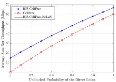
(a)

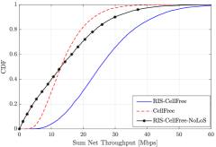
(b)

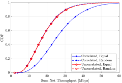
(c)

Figure 2: The sum net throughput [Mbps]: $(a)$ Average sum net throughput versus the unblocked probability of the direct links; $(b)$ CDF of the sum net throughput with the unblocked probability of the direct links $\tilde{p}=0.2$; $(c)$ Sum net throughput as a function of the phase shift setup (equal or random) and the unblocked probability of the direct links $\tilde{p}=0.2$.

IV Numerical Results

We consider a geographic area of size $1$ km² that is wrapped around at the edges. The locations of $100$ APs and $10$ users are given in terms of $(x,y)$ coordinates. To simulate a harsh communication environment, the APs are uniformly distributed in the sub-region $x,y\in[-0.75,-0.5]$ km, while the users are uniformly distributed in the sub-region $x,y\in[0.375,0.75]$ km. An RIS with $N=900$ is located at the origin, i.e., $(x,y)=(0,0)$. Each coherence interval comprises $\tau_{c}=200$ symbols and $\tau_{p}=5$ orthonormal pilot sequences. The large-scale fading coefficients $\alpha_{m}$ and $\tilde{\alpha}_{mk}$ are generated according to the three-slope propagation model in [2]. The large-scale fading coefficient $\beta_{mk}$ is formulated as $\beta_{mk}=\bar{\beta}_{mk}a_{mk},$ where $\bar{\beta}_{mk}$ is generated by the three-slope propagation model in [2]. The binary variables $a_{mk}$ accounts for the probability that the direct links are unblocked, and it is defined as $a_{mk}=1$ with probability $\tilde{p}$. Otherwise, $a_{mk}=0$ with probability $1-\tilde{p}$, where $\tilde{p}\in[0,1]$ is the probability that the direct link is not blocked.The covariance matrices are generated according to the spatial correlation model in (2) with $d_{H}=d_{V}=\lambda/4$. The pilot power is $100$ mW and $\nu=1$. The power control coefficients are $\eta_{k}=1,\forall k$. Without loss of generality, in particular, the $N$ phase shifts in $\boldsymbol{\Phi}$ are all set equal to $\pi/4$, except in Fig. 2(c) with different phase shifts. Three system configurations are considered for comparison:

• RIS-Assisted Cell-Free Massive MIMO: This is the proposed system model where the direct links are unblocked with probability $\tilde{p}$. It is denoted by “RIS-CellFree”.

• Conventional Cell-Free Massive MIMO: This is the same as the previous model with the only exception that the RIS is not deployed. It is denoted by “CellFree”.

• Cell-Free Massive MIMO without the direct links: This is the worst case study in which the direct links are blocked with unit probability and the uplink transmission is ensured only through the RIS. This setup is denoted by “RIS-CellFree-NoLOS”.

In Fig. 2(a), we illustrate the sum net throughput as a function of the probability $\tilde{p}$. In particular, the average sum net throughput is defined as $\sum_{k=1}^{K}\mathbb{E}\{R_{k}\}$. Cell-Free Massive MIMO provides the worst performance if the blocking probability is large ($\tilde{p}$ is small). If the direct links are unreliable, as expected, the net throughput offered by Cell-Free Massive MIMO tends to zero if $\tilde{p}\rightarrow 0$. In addition, the proposed RIS-assisted Cell-Free Massive MIMO setup offers the best net throughput, since it can overcome the unreliability of the direct links. An RIS is particularly useful if $\tilde{p}$ is small since in this case the direct links are not able to support a high throughput. Fig. 2(b) compares the three considered systems in terms of sum net throughput (defined as $\sum_{k=1}^{K}R_{k}$) when $\tilde{p}=0.2$. We observe the net advantage of the proposed RIS-assisted Cell-Free Massive MIMO system. The worst-case RIS-assisted Cell-Free Massive MIMO system setup (i.e., $\tilde{p}=0$) outperforms the Cell-Free Massive MIMO setup in the absence of an RIS. Fig. 2(c) focuses on the RIS-asissted Cell-Free Massive MIMO setup, since it provides the best performance. We compare the sum net throughput as a function of the phase shifts of the RISs (random and uniform phase shifts according to Corollary 1 in the presence of spatially-correlated and spatially-independent fading channels according to (2). In the presence of spatial correlation, we consider $\mathbf{R}_{m}=\alpha_{m}d_{H}d_{V}\mathbf{I}_{N}$ and $\widetilde{\mathbf{R}}_{k}=\tilde{\alpha}_{k}d_{H}d_{V}\mathbf{I}_{N},\forall m,k$. If the spatial correlation is not considered, there is no significant difference between the random and uniform phase shifts setup. In the presence of spatial correlation, on the other hand, the proposed uniform phase shift design, which is obtained from Corollary 1, provides a much better throughput. This result highlights the relevance of using even simple optimization designs for RIS-assisted communications in the presence of spatial correlation.

V Conclusion

We have considered an RIS-assisted Cell-Free Massive MIMO system and have introduced an efficient channel estimation scheme to overcome the high channel estimation overhead. An optimal design for the phase shifts of the RIS that minimizes the channel estimation error has been introduced and has been used for system analysis. Also, a closed-form expression of the ergodic net throughput for the uplink data transmission phase has been proposed. Based on them, the performance of RIS-assisted Cell-Free Massive MIMO has been analyzed as a function of the fading spatial correlation and the blocking probability of the direct AP-user links. The numerical results have shown that the presence of an RIS is very useful if the AP-user links are mostly unreliable with high probability.

References

- [1] T. V. Chien, H. Q. Ngo, S. Chatzinotas, M. Di Renzo, and B. Otternsten, “Reconfigurable intelligent surface-assisted Cell-Free Massive MIMO systems over spatially-correlated channels,” IEEE Trans. Wireless Commun., 2021, submitted for publication.
- [2] H. Q. Ngo, A. Ashikhmin, H. Yang, E. G. Larsson, and T. L. Marzetta, “Cell-free massive MIMO versus small cells,” IEEE Trans. Wireless Commun., vol. 16, no. 3, pp. 1834–1850, 2017.
- [3] T. A. Le, T. Van Chien, and M. Di Renzo, “Robust probabilistic-constrained optimization for IRS-aided MISO communication systems,” IEEE Wireless Commun. Lett., vol. 10, no. 1, pp. 1–5, 2021.
- [4] M.-M. Zhao, Q. Wu, M.-J. Zhao, and R. Zhang, “Intelligent reflecting surface enhanced wireless network: Two-timescale beamforming optimization,” IEEE Trans. Wireless Commun., 2020.
- [5] N. S. Perović, L.-N. Tran, M. Di Renzo, and M. F. Flanagan, “Achievable rate optimization for MIMO systems with reconfigurable intelligent surfaces,” IEEE Trans. Wireless Commun., vol. 20, no. 6, pp. 3865 – 3882, 2021.
- [6] T. Zhou, K. Xu, X. Xia, W. Xie, and J. Xu, “Achievable rate optimization for aerial intelligent reflecting surface-aided Cell-Free Massive MIMO system,” IEEE Access, 2020.
- [7] Z. Zhang and L. Dai, “Capacity improvement in wideband reconfigurable intelligent surface-aided cell-free network,” in Proc. IEEE SPAWC, 2020, pp. 1–5.
- [8] T. Van Chien, A. K. Papazafeiropoulos, L. T. Tu, R. Chopra, S. Chatzinotas, and B. Ottersten, “Outage probability analysis of IRS-assisted systems under spatially correlated channels,” IEEE Wireless Commun. Lett., 2021.
- [9] Q. Wu and R. Zhang, “Intelligent reflecting surface enhanced wireless network via joint active and passive beamforming,” IEEE Trans. Wireless Commun., vol. 18, no. 11, pp. 5394–5409, 2019.
- [10] E. Björnson and L. Sanguinetti, “Rayleigh fading modeling and channel hardening for reconfigurable intelligent surfaces,” IEEE Wireless Commun. Lett., vol. 10, no. 4, pp. 830 – 834, 2021.
- [11] T. Van Chien, E. Björnson, and E. G. Larsson, “Joint power allocation and load balancing optimization for energy-efficient cell-free Massive MIMO networks,” IEEE Trans. Wireless Commun., vol. 19, no. 10, pp. 6798–6812, 2020.
- [12] S. Kay, Fundamentals of Statistical Signal Processing: Estimation Theory. Prentice Hall, 1993.
- [13] H. Cramér, Random variables and probability distributions. Cambridge University Press, 2004, vol. 36.