Not All Negatives are Equal:
Label-Aware Contrastive Loss for Fine-grained Text Classification

Abstract

Fine-grained classification involves dealing with datasets with larger number of classes with subtle differences between them. Guiding the model to focus on differentiating dimensions between these commonly confusable classes is key to improving performance on fine-grained tasks. In this work, we analyse the contrastive fine-tuning of pre-trained language models on two fine-grained text classification tasks, emotion classification and sentiment analysis. We adaptively embed class relationships into a contrastive objective function to help differently weigh the positives and negatives, and in particular, weighting closely confusable negatives more than less similar negative examples. We find that Label-aware Contrastive Loss outperforms previous contrastive methods, in the presence of larger number and/or more confusable classes, and helps models to produce output distributions that are more differentiated.

1 Introduction

Fine-grained classification involves distinguishing between classes that have subtle variations among them. For example, in image classification, we can classify birds from non-birds, or attempt a more fine-grained classification of bird species Akata et al. (2015). In NLP, one example is sentiment analysis, where we could have a coarse positive/negative classification, or a fine-grained set of categories that differentiate “positive” and “very positive” (i.e., an ordinal scale), such as in Socher et al. (2013). Similarly, for emotion classification, we could try to classify a text into 4 to 6 emotions, or into much finer classifications of 27 Demszky et al. (2020) or 32 Rashkin et al. (2019) emotion categories. This involves distinguishing between some closely confusable pairs of emotions, such as “sad” and “devastated”, or “furious” and “annoyed”. Fine-grained classification tasks are challenging precisely due to the presence of class interference amongst closely confusable classes Collins et al. (2018); Zhao et al. (2017).

The standard approach today to task classification involves using a pre-trained language model (e.g., BERT) which is fine-tuned on downstream tasks using a standard cross-entropy loss. However, this standard loss may not be the optimal manner in which to train fine-grained classification models. A simple counterexample is that cross-entropy loss treats misclassifications as nominal, not ordinal, so misclassifying a “positive” as a “very positive” is no worse (in terms of the loss) as “very negative”. But even within nominal categories, misclassifying “annoyed” as “furious” is quite different from a misclassification of “joyful”, as there are varying degrees of semantic similarity between nominal categories. Intuitively, we can try to improve model performance by modifying the loss to reflect the contrast between pairs of examples of the same or different classes. Such contrastive approaches are widely used in computer vision tasks for label-noise reduction, semi-supervised and self-supervised learning tasks Le-Khac et al. (2020). More recently in NLP, Gunel et al. (2021) used a supervised contrastive loss to improve fine-tuning performance of pre-trained language models in several few-shot learning scenarios.

In this work, we incorporate inter-class relationships into a Label-aware Contrastive Loss (LCL), which helps the model to differentiate the weights between different negative samples. At a high level, the model adaptively learns which pairs of classes are more similar, and which are more different. We use a dual-model approach where a weighting model learns the inter-label relationships that are used in the main embedding model’s contrastive objective. We evaluate our approach on two popular tasks in NLP: emotion recognition (4 datasets to span both coarse- and fine-grained classification), and sentiment analysis (with a coarse and fine-grained version of the same dataset). We find that LCL outperforms existing contrastive learning losses, and performs comparably with the state-of-the-art. We supplement our findings with targeted experiments to provide evidence for boundary conditions—situations in which LCL should work best—and for how LCL affects model prediction confidence.

2 Related Work

2.1 Fine-grained classification

Fine-grained classification is a popular problem in image classification, including tasks like distinguishing between different animal species Wei et al. (2019); Zhao et al. (2017). We note that in NLP, “fine-grained” is commonly used when analysing different granularities of text, such as character-, word- and span-level information Zirn et al. (2011); Da San Martino et al. (2019); Liu et al. (2020). In this work, we use fine-grained classification to refer to the nature of labels associated with the task.

Fine-grained classification tasks involve finding subtle differences to distinguish between close classes. For instance, “coarse" sentiment classification involves distinguishing negative and positive sentiments in text, and fine-grained sentiment classification involves further distinguishing the positive class into very positive and positive. This problem is challenging because the classes are semantically similar, which makes it difficult for the model to learn the labels Collins et al. (2018).

Recent models have applied state-of-the-art attention mechanisms and multi-task learning to solve fine-grained sentiment classification. Balikas et al. (2017) performed fine-grained sentiment classification using a multi-task learning setup that performed both binary and fine-grained sentiment classification simultaneously. Yin et al. (2020) composed the sentiment semantics using an attention network to enhance BERT’s pre-training objective, and showed improvement in a downstream fine-grained sentiment analysis task. Tian et al. (2020a) modified the pre-training objectives of language models to include more sentiment-specific tasks, such as sentiment word masking and sentiment word prediction, and showed improved performance in fine-grained sentiment analysis. These previous methods mostly focus on improving the pre-training of language models, or incorporating multiple task training; here, we focus on improving contrastive fine-tuning to solve fine-grained text classification.

Another important fine-grained classification task is that of emotion recognition. Traditionally, emotion recognition datasets have a small number of emotions (e.g., 4-7). Two recent datasets were proposed to address this issue: Rashkin et al. (2019) introduced Empathetic Dialogues, which contains text conversations labelled with 32 emotion labels, and Demszky et al. (2020) introduced GoEmotions, which contains Reddit comments labelled with 27 emotion labels. Recently, Suresh and Ong (2021) introduced a method to incorporate knowledge from emotion lexicons into an attention mechanism to improve fine-grained emotion classification on these two datasets. Khanpour and Caragea (2018) similarly used lexicon-based features to tackle fine-grained emotion recognition from online health posts. However, there is still much work to be done in fine-grained emotion classification, and it has important implications for designing empathetic agents and chatbots Roller et al. (2021).

Finally, we note that fine-grained classification has also been explored in the context of entity-type classification Ling and Weld (2012); Jin et al. (2019). However, this task is generally multi-label in nature and is out of the scope of the current work.

2.2 Contrastive learning

Contrastive learning focuses on improving the ability of the model to differentiate a given data point from “positive” examples (points sharing the same label) and from “negative” examples (different labels). Contrastive learning has been widely used in computer vision, especially in self-supervised settings Le-Khac et al. (2020); Chen et al. (2020) where such learning guides the model based on similarities between the latent representation of the samples. Chen et al. (2020) introduced SimCLR, a simplified version of contrastive loss that does not use memory banks Tian et al. (2020b); He et al. (2020); Misra and Maaten (2020) or designated architectures Bachman et al. (2019), and which achieves improved performance in both semi-supervised and self-supervised settings. SimCLR uses data augmentation to create “positive” examples that are similar to a given input. Khosla et al. (2020) extended SimCLR to also leverage label information: they include other training examples with the same label in the set of “positive” examples.

Contrastive loss has also been recently incorporated in both the pre-training and fine-tuning objectives of pre-trained language models. Self-supervised contrastive loss has been used for pre-training language models such as BERT Fang and Xie (2020); Meng et al. (2021). Gunel et al. (2021) used a combination of cross entropy and supervised contrastive loss for fine-tuning pre-trained language models to improve performance in few-shot learning scenarios. Gao et al. (2021) used a contrastive objective to fine-tune pre-trained language models to obtain sentence embeddings, and achieved state-of-the-art performance in sentence similarity tasks. In our work, we aim to improve the fine-tuning objective of pre-trained language models for downstream tasks involving fine-grained classes.

2.3 Other related work

In addition to the above works, we mention other related references which used similar techniques. Dual-model approaches are used in tasks like knowledge distillation, where the knowledge from a larger teacher network is transferred to a lighter student model Hinton et al. (2015); Kim and Rush (2016); Sun et al. (2020, 2019); Li et al. (2020); Aguilar et al. (2020), however, these works are mainly focused on model compression. Dual-model strategies have also been widely used in label-noise representation learning in image classification tasks Han et al. (2018); Wei et al. (2020); Lu et al. (2021); Feng et al. (2019) by updating each other with clean samples (the samples which have the lowest loss value in every iteration). However, the sample selection performed by these works assume that the noise rate in each dataset is known or needs to be estimated, which is not always possible.

Another set of works focus on sample re-weighting to focus on select samples more. Plank et al. (2014) use inter-annotator agreement to guide the model’s focus on samples that are harder to distinguish. Sample re-weighting is also widely used to reduce label noise. Although the majority of works in this area depend on a pre-determined weighting function, there are a few notable papers which automate this process by adaptively calculating weights: Chang et al. (2017) uses active learning to re-weight samples, while Ren et al. (2018) uses gradients to learn weights, however their performance drops with large number of classes Song et al. (2020). Meta-Weight-Net uses a single-layer neural network to obtain the weights Shu et al. (2019). These methods all require clean validation data to optimize their learning objective.

3 Approach

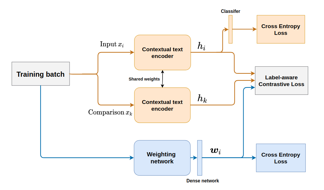
Figure 1: Illustration of training strategy used in our Label-aware Contrastive Loss approach. The encoder network is in orange and the the weighting network is indicated in blue. In the encoder network, every sample from the training batch is compared against every other sample in the Label-aware Contrastive Loss function. Note that at testing time, only the contextual encoder is used.

3.1 Contrastive Loss

A Contrastive Loss (CL) brings the latent representations of samples belonging to the same class closer together, by defining a set of positives (that should be closer) and negatives (that should be further apart). The type of positives and negatives vary and is dependent on the contrastive loss used. Throughout this section we denote the set of positives as $\mathcal{P}$ and set of negatives as $\mathcal{N}$. Let us also denote a batch of sample and label pairs as $\{x_{i},y_{i}\}_{i\in I}$, where $I=\{1,\cdots,K\}$ is the indices of the samples and $K$ is the batch-size.

In the self-supervised version of contrastive loss Chen et al. (2020), one applies augmentation to all $K$ samples to produce $K$ augmented data-points. Therefore, the batch size becomes $2K$ and $I=\{1,\cdots,2K\}$. The positive set for a given $x_{i}$ contains only one sample, the augmented version of $x_{i}$, and we denote its index as $g(i)$. The negative set would be the rest of the samples in the batch. The loss is defined as:

$$L_{self}=\sum_{i=1}^{2K}-\log\frac{\exp(h_{i}\cdot h_{g(i)}/\tau)}{\sum_{k\in\mathcal{I}/i}\exp(h_{i}\cdot h_{k}/\tau)}$$ (1)

where $\tau$ is the temperature hyper-parameter. Larger values of $\tau$ scale down the dot-products, creating more difficult comparisons. $h_{i}$ is the normalised representation vector of $x_{i}$ obtained from an encoder $\Phi$.

Khosla et al. (2020) extended the above loss to a Supervised Contrastive Loss (SCL) by including the samples belonging to the same class as $x_{i}$ in its positive set. The positive set is given by $\mathcal{P}=\{p:{p\in I},{y_{p}=y_{i}}\land p\neq i\}$, with size $|\mathcal{P}|$. The supervised contrastive loss is given by:

$$L_{SCL}=\sum_{i=1}^{2K}\frac{-1}{|\mathcal{P}|}\sum_{p\in\mathcal{P}}\log\frac{\exp(h_{i}\cdot h_{p}/\tau)}{\sum_{k\in\mathcal{I}/i}\exp(h_{i}\cdot h_{k}/\tau)}$$ (2)

3.2 Label-aware Contrastive Loss

In our work, we introduce relationships between class labels to adaptively distinguish between the negative examples. From Eqn. 2 we can see that Supervised Contrastive Loss weights all positive and negative samples equally to the current sample $x_{i}$. But not all negatives are equal. In certain fine-grained text classification tasks, we have semantically-similar labels with more subtle differences, and are thus more confusable. For example, “sad” and “devastated” are semantically closer emotion categories than “sad” and “happy”. Thus, our goal was to introduce a method for adaptively weighting a given input’s positive/negative samples based on the label-relationships between them, thereby helping the model differentiate the more difficult negatives.

We propose Label-aware Contrastive Loss (LCL) which adapts Contrastive Loss for fine-grained classification tasks by incorporating inter label-relationships. For the positive set, we follow Khosla et al. (2020); Gunel et al. (2021) where $\mathcal{P}$ of a given sample contains the augmented sample and samples within the same class. We utilise a weighting vector $\boldsymbol{w_{i}}\in\mathbb{R}^{C}$ where $C$ is total number of classes to weight the pair-wise similarity values of the supervised contrastive loss defined in Eq. 2. Our adapted loss function for each entry $i$ and total across the batch is:

$$\mathcal{L}_{i}=\sum_{p\in\mathcal{P}}\log\frac{w_{i,y_{i}}\cdot\exp(h_{i}\cdot h_{p}/\tau)}{\sum_{k\in\mathcal{I}\setminus i}w_{i,y_{k}}\cdot\exp(h_{i}\cdot h_{k}/\tau)}$$ (3)

$$L_{LCL}=\sum_{i=1}^{2K}\frac{-1}{|\mathcal{P}|}\mathcal{L}_{i}$$ (4)

Here, $w_{i,y_{k}}$ indicates the relationship between an input $x_{i}$ and a label $y_{k}$. Just as in the previous losses, $h_{i}\in\mathbb{R}^{d}$ is the output representation of the encoder for $x_{i}$. We normalise $h_{i}$ for the similarity comparison, similar to Chen et al. (2020).

In contrastive loss we want the weights of the positives to be higher and that of the negatives to be lower. However, we want to increase the weight of confusable negative labels relative to other negative labels. In our work, we aim to incorporate these inter-label relationships into the contrastive objective. To weigh each comparison sample differently, in addition to a primary encoder $\Phi$, we use a weighting network $\Psi$. We follow a dual-model strategy similar to co-teaching approaches Han et al. (2018); Wei et al. (2020) where the weighting network is a second network that coordinates with the primary encoder. The input batch is fed into $\Psi$ and output is optimised using Cross-entropy loss $L_{w}$. The prediction probabilities obtained from the softmax layer, i.e. soft labels, is used to obtain confidence of the current sample, is given by:

$$\boldsymbol{w_{i}}=\frac{\exp(h_{i})}{\sum_{c=1}^{C}\exp(h_{i})}$$ (5)

Here, $\boldsymbol{w_{i}}=\{w_{i,c}\}_{c=1}^{C}$ where $C$ is the total number of classes. Each $w_{i,c}$ denotes the confidence of the weighting network that sample $x_{i}$ belongs to class $c$. When $\Psi$ is given a confusable sample, it will have higher scores for the classes that are more closely associated with the current sample. We hypothesize that incorporating these high values back into the negative comparison in the supervised contrastive loss of the primary encoder would steer the encoder toward finding more distinguishing patterns to differentiate between confusable samples.

Training setup: The output vector of the weighting network is optimized using a Cross Entropy Loss $L_{w}$, while the output of the encoder network is optimized by using a linear combination of $L_{LCL}$ and Cross Entropy Loss $L_{e}$. The encoder and weighting networks are jointly optimised using objective function $L_{f}$:

$$L_{f}=\alpha(L_{w}+L_{e})+(1-\alpha)L_{LCL}$$ (6)

Here, $\alpha$ is a tunable loss scaling factor similar to Gunel et al. (2021). We note that both the encoder and the weighting network are utilised during training, but in the testing phase, we use only the primary encoder network.

The overall training process is shown in Fig. 1. Each input training batch $I$ is passed to the encoder network $\Phi$ and the weighting network $\Psi$ simultaneously. Here, both these networks are initialised by a pre-trained language model and the [CLS] token of the last layer of $\Phi$ is the final representation $h_{i}$ which is used for computing $L_{LCL}$. For performing the classification, $h_{i}$ is projected down using the classifier and the output is optimised using cross-entropy loss $L_{e}$. The architecture of the weighting network was designed in the same way as the fine-tuning setup of the pre-trained language model of choice, and the weight vector $\boldsymbol{w}_{i}$ is the output probability vector obtained after the softmax projection.

4 Experiments

4.1 Datasets

We evaluate our approach using two tasks, Emotion Recognition and Sentiment Analysis. We choose these tasks as it helps demonstrate our model’s performance in different types of inter-class relationships that exist in text classification. Specifically, in sentiment classification the classes are ordinal, whereas in emotion recognition the classes are nominal.

For emotion recognition, we use the following 4 datasets, ordered in decreasing number of classes:

• Empathetic Dialogues Rashkin et al. (2019): a dataset of two-way conversations between a speaker and listener, and labelled with 32 emotions. In this work, we only use the first turn of the conversation, which consists of the speaker describing an emotional incident. The train/validation/test split for the dataset is 19,533 / 2,770 / 2,547 samples respectively.

• GoEmotions Demszky et al. (2020), a dataset of Reddit comments labelled with 27 emotions (we did not include samples with neutral label). The original dataset is multi-labelled, i.e, some samples have more than one label. In this work, we use only the single-labelled samples, which is $\sim$80% of the total data. The train/validation/test split of this dataset is 23,485 / 2,956 / 2,984.

• ISEAR (International Survey on Emotion Antecedents and Reactions) Scherer and Wallbott (1994) contains sentences of emotion experiences labelled with one of 7 emotion categories. The train/validation/test split of the dataset is 4,599 / 1,533 / 1,534.

• EmoInt Mohammad and Bravo-Marquez (2017) consists of tweets labelled with one of 4 emotion categories. The train/validation/test split of this dataset is 3,612 / 346 / 3,141.

For Sentiment Analysis, we use the 5-class and 2-class classification versions of the Standford Sentiment Treebank Socher et al. (2013), which consists of movie reviews annotated for sentiment. The SST-5 has 5 classes (very negative, negative, neutral, positive, and very positive), while the SST-2 is only a binary (negative/positive) classification. The train/validation/test split for the SST-5 is 8,544/ 1,101 / 2,210, and for SST-2 is 6,920 / 872 / 1,821.

4.2 Implementation Details

We initialised both the pre-trained encoder and weighting network using $\text{ELECTRA}_{base}$ (electra-base-discriminator) from HuggingFace’s Transformers library Wolf et al. (2020), which consists of 12 Transformer layers with a hidden representation size of 768. As is convention, we use the representation corresponding to the [CLS] token of the last layer as an input into the final classification layer Clark et al. (2019). The classifier present in the primary encoder consists of a 2-layer dense network with the first layer having hidden size of 768 with a ReLU activation, followed by an output layer. The dropout was set to 0.1.

Similar to previous research Khosla et al. (2020); Gunel et al. (2021), we use data augmentation to generate positive samples. Here, we use synonym replacement where we substitute 30% of the words in the input text by replacing it with words with semantic similarity using WordNet dictionary Miller (1995). The coverage of the WordNet dictionary was $\sim$69% for EmpatheticDialogues, $\sim$69% for SST-2 and SST-5, $\sim$66% for ISEAR, $\sim$62% for EmoInt and $\sim$61% for GoEmotions. Previous research Wei and Zou (2019) have shown that synonym replacement works well as it could introduce new vocabulary words and help the model generalise. In addition, synonym replacement does not require an external model unlike other augmentation methods like back-translation.

For training, we used the Adam optimiser and early stopping based on performance on the validation set. We ran our models with 5 random seed settings and report the mean performance. More details regarding the hyper-parameter settings and computing infrastructure can be found in the Appendix. Source code is available at https://github.com/varsha33/LCL_loss.

4.3 Model comparisons and evaluation

For the emotion classification task we calculate classification accuracy and F1 score, while for sentiment analysis we compare accuracy of sentence-level sentiment classification. For both tasks, we compare LCL against the following baselines:

• Fine-tuning objectives: We compare against the standard Cross-entropy Loss, as well as Supervised Contrastive Loss (SCL) Gunel et al. (2021). In both comparisons and in LCL, we use $\text{ELECTRA}_{base}$ as the pre-trained language model.

• General pre-trained language models: For emotion classification, we also compare with $\text{BERT}_{base}$ Devlin et al. (2019) as our baseline. We use the same fine-tuning architecture as Devlin et al. (2019). For sentiment analysis, we compare against $\text{BERT}_{base}$ (SST-2 Devlin et al. (2019) and SST-5 Munikar et al. (2019)) and $\text{RoBERTa}_{base}$ Liu et al. (2019).

• Sentiment-specific language models: For sentiment analysis, we compare against SentiBERT Yin et al. (2020), SentiLARE Ke et al. (2020) and SKEP Tian et al. (2020a), which are language models designed specifically for sentiment analysis and related tasks.

5 Results and Discussion

Dataset:	Empathetic Dialogues		GoEmotions		ISEAR		EmoInt
Number of classes:	32		27		7		4
	Acc / %	F1	Acc / %	F1	Acc / %	F1	Acc / %	F1
$\text{BERT}_{base}$	55.8 (0.8)	54.4 (1.2)	64.1 (0.5)	63.0 (0.9)	69.2 (0.3)	69.3 (0.1)	85.0 (0.6)	85.0 (0.6)
ELECTRAbase + Cross-Entropy Loss	58.3 (0.5)	56.8 (0.5)	64.8 (0.3)	63.9 (0.4)	71.4 (0.2)	71.4 (0.2)	85.5 (0.9)	85.5 (0.9)
ELECTRAbase + SCL Gunel et al. (2021)	58.5 (0.7)	57.0 (0.9)	64.3 (0.4)	63.0 (0.4)	70.5 (0.5)	70.5 (0.6)	85.7 (0.2)	85.8 (0.2)
ELECTRAbase + LCL	60.1 (0.3)	59.1 (0.3)	65.5 (0.2)	64.8 (0.2)	72.4 (0.2)	72.4 (0.2)	86.6 (0.3)	86.6 (0.3)

Table 1: Summary of results for fine-grained emotion recognition. We divide the table into fine-grained (left) and coarse-grained (right) emotion classification, based on the number of classes. We compare the results of an ELECTRA encoder trained with: a standard cross-entropy loss, a Supervised Contrastive Loss (SCL), and our proposed Label-aware Contrastive Loss (LCL). The results shown are averaged over 5 runs, with standard deviations in parenthesis.

5.1 Emotion Classification Performance

For emotion classification we compared our proposed Label-aware Contrastive Loss (LCL) work with the standard training objective, i.e., cross-entropy loss. We also compared with Gunel et al. (2021)’s formulation of Supervised Contrastive Loss (SCL), who used a linear combination of SCL and Cross-entropy loss for fine-tuning pre-trained language models (in contrast to the original SCL paper, Khosla et al., 2020, who used a two-stage training regime). For all fine-tuning objectives, we used $\text{ELECTRA}_{base}$ as the pre-trained language model. To evaluate the approaches we use top-1 Accuracy and weighted macro F1-score.

As shown in Table 1, our LCL objective function improved classification performance compared to both SCL and cross-entropy loss, on both fine-grained emotion classification (32-class, LCL$>$SCL, t-test on accuracy, $t=4.20,p=.007$, LCL$>$CEL, $t=6.42,p<.001$; and 27-class classification; LCL$>$SCL, $t=5.70,p<.001$, LCL$>$CEL, $t=4.32,p=.002$), as well as coarse-grained emotion classification (7-class, LCL$>$SCL, $t=7.39,p<.001$, LCL$>$CEL, $t=7.70,p<.001$; and 4-class classification, LCL$>$SCL, $t=5.34,p<.001$, LCL$>$CEL, $t=2.25,p=.078$ not significant). The consistent improved performance of LCL is in contrast to SCL, which did not outperform standard cross-entropy loss, (all $p>.05$, with SCL in fact performing worse than CEL on ISEAR, $t=3.34,p=.02$). These results suggest that incorporating class relationships into the fine-tuning objective of pre-trained language models can improve classification accuracies.

5.2 Sentiment Analysis Performance

	SST-5	SST-2
	Acc / %	Acc / %
$\text{BERT}_{base}$ Munikar et al. (2019)	53.2 (-)
$\text{BERT}_{base}$Devlin et al. (2019)		93.5(-)
$\text{RoBERTa}_{base}$ Liu et al. (2019)	56.2 (-)	94.8(-)
SentiBERTYin et al. (2020)	57.8 (-)	94.7 (-)
SentiLAREKe et al. (2020)	58.6 (-)
SKEP Tian et al. (2020a)		96.7 (-)
$\text{ELECTRA}_{base}$Clark et al. (2019)		93.4 (-)
$\text{ELECTRA}_{base}$ (Our implementation)	57.1 (1.2)	94.4 (0.3)
$\text{ELECTRA}_{base}$+ SCL Gunel et al. (2021)	57.4 (0.6)	94.3 (0.2)
$\text{ELECTRA}_{base}$ + LCL (Ours)	58.5 (0.2)	94.5 (0.1)

Table 2: Summary of results for fine-grained (5-class) and coarse-grained (2-class) sentiment analysis. The results shown are averaged over 5 runs, with standard deviations in parenthesis.

For sentiment analysis, we used the sentence inputs from SST-5 and SST-2. In addition to comparing LCL with varying fine-tuning objectives (cross-entropy and SCL), we also compare against recent state-of-the-art works, focusing on pre-trained language models and pre-trained language models learnt specifically for sentiment classification such as SentiBERT Yin et al. (2020), SentiLARE Ke et al. (2020), and SKEP Tian et al. (2020a). To ensure a fair comparison, we use the $base$ version of the pre-trained language models unless mentioned otherwise. To evaluate, we use top-1 Accuracy.

From the results in Table 2, in the case of SST-5, our LCL objective showed improved classification performance compared to SCL ($t=3.61,p=.01$), and standard cross-entropy loss (SST-5: $t=2.40,p=.069$, although this is not significant due to high SD in CEL performance). Our LCL-fine-tuned model also achieves a performance comparable to the state-of-the-art performance of SentiLARE, although not statistically different ($p=.77$). On SST-2, our LCL performance gains compared to cross-entropy and SCL are far more modest (neither were statistically significant; $p=.78$ and $p=.32$ respectively), and it performs comparably to previous SOTA pre-trained models, although it does not do as well as SKEP ($p<.001$). We provide two possible reasons: one, there is already very high performance (e.g. 94% accuracies) on this binary classification task, which makes it difficult to get clear consistent improvements. Second and more importantly, we designed LCL to increase inter-class contrast, and so our method should work better for higher number of classification, compared to binary classification. Indeed, we see that LCL’s improvements are much stronger and consistent on the fine-grained (5-class) sentiment classification task.

5.3 Case Study: Varying number of classes

Number of classes:	32	16	8	4-easy	4hard-a	4hard-b	4hard-c	4hard-d
Cross-Entropy Loss	58.1 (0.7)	68.8 (0.4)	78.0 (0.6)	89.2 (0.3)	56.1 (0.5)	63.2 (0.9)	54.3 (1.0)	67.4 (0.6)
Supervised Contrastive Loss	58.6 (0.5)	67.9 (0.6)	77.0 (0.8)	88.8 (0.5)	55.4 (0.5)	63.7 (1.1)	53.3 (0.8)	68.1 (0.7)
Label-aware Contrastive Loss	60.1 (0.2)	69.6 (0.5)	78.7 (0.4)	88.8 (0.6)	57.5 (0.7)	64.2 (0.7)	55.6 (0.6)	69.5 (0.5)

Table 3: Case study using class subsets of EmpatheticDialogues. For brevity, we only report accuracy scores. Column headers give the number of class labels in that comparison. 4-easy denotes a coarse-grained set of four emotions that are more easily distinguishable (on which we predicted that LCL would not add much), while the 4-hard sets denote fine-grained sets of four emotions that are semantically more similar. Results shown are averaged over 10 runs, with standard deviations in parentheses.

We designed LCL to increase inter-class contrast, and we see marked improvements for all the tasks studied except for the 2-class (SST-2) classification. We hypothesized that LCL should do better with an increasing number of classes, but unfortunately it is difficult to draw that inference from Tables 1 and 2 as each dataset only provides one datapoint about number of classes, and there are also differences across datasets which is difficult to control for. Thus, in this experiment, we used the dataset with the largest number of emotion classes, Empathetic Dialogues (with 32-classes), and subsampled some fraction of emotion classes from this dataset to create “mini-datasets” of differing number of emotion classes. This allows us to systematically vary the number of classes that our LCL-tuned model has to learn to classify, and examine the performance of the model. We predict that LCL will have a greater contribution to performance when (i) the number of classes is larger, and (ii) the classes are more confusable.

The full dataset has 32-classes. We randomly sampled a partition of 16 emotions, and 8 emotions. We also created several subsets of 4-emotions. We designed a “4-easy” with 4 widely separated emotion classes (4-easy: {Angry, Afraid, Joyful, Sad}) which are the same classes as EmoInt and comprise a subset of Ekman (1999)’s list of six “basic" emotions. (We predicted that LCL would not perform too well on this easy subset).

We adopted a data-driven approach to pick the “hard" subsets by picking the most-confusable sets of 4 emotions. First, we trained a standard cross-entropy loss model (similar to our weighting network in LCL in Fig.1), to obtain the 32-by-32 confusion matrix, which gives us an estimate of how confusable each pair of classes is. We exhaustively enumerated all 35,960 (32-choose-4) 4-class combinations: For each combination we extracted the corresponding 4x4 sub-matrix of the 32-by-32 confusion matrix, and calculated the sum of the off-diagonal elements of the 4x4 sub-matrix. The highest confusable combination of emotions was (4-hard-a: {Anxious, Apprehensive, Afraid, Terrified}). After excluding these emotions, the next-most confusable combinations were (4-hard-b: {Devastated, Nostalgic, Sad, Sentimental}), (4-hard-c: {Angry, Ashamed, Furious, Guilty}), and (4-hard-d: {Anticipating, Excited, Hopeful, Guilty}). We predicted that for all of these “hard" sets that contain confusable emotions, LCL should outperform the other methods.

The results from this case study are given in Table 3. For the 32, 16, and 8-class classification, as we predicted, we see a robust and consistent improvement of our proposed LCL over SCL and cross-entropy loss (16 classes: LCL$>$SCL, $t=6.28,p<.001$; LCL$>$CEL, $t=3.82,p=.001$; 8 classes: LCL$>$SCL, $t=6.27,p<.001$; LCL$>$CEL, $t=3.16,p=.007$). For the easy 4-class classification where the classes are conceptually “far apart”, and hence, contrastive learning should not add much, we see that all three methods perform identically well ($p>.15$). But when we consider the more difficult 4-class classifications where the classes are much more conceptually similar, then LCL outperforms the other two methods by a statistically-significant margin (all $p$’s $<.05$ except for LCL and SCL in 4-hard-b because of the high SD’s in that comparison). Thus, our results provide evidence that LCL is an effective fine-tuning strategy, especially when there are a large number of highly-similar classes.

5.4 Quantifying model confidence

Finally, we wanted to try to quantify the intuition that LCL helps to reduce the confusion among confusable classes. Beyond looking at the top-1 accuracy, we turned to the distribution of prediction scores among the different emotion classes. If LCL helps the model to better differentiate emotion classes, then we should also see this in the distribution of prediction scores for the different classes. For example, consider an example where devastated is the model’s predicted label, and sad is a closely confusable class; if LCL helps to sharpen the model’s ability to differentiate closely confusable classes, then the model’s prediction score for devastated should also be much higher than that for sad. In general, we predict that LCL would result in more “peaky” distributions.

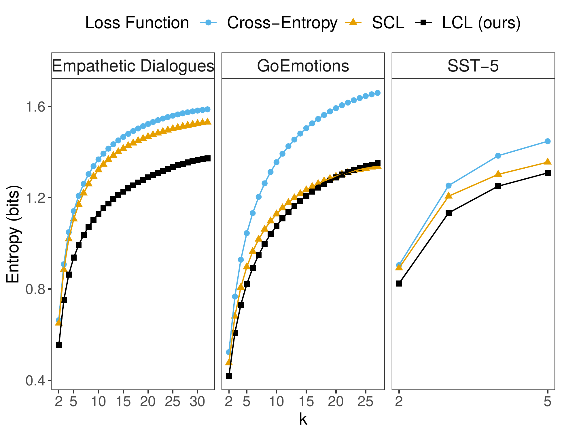
Figure 2: Averaged entropy of the prediction score distributions, for the top-$k$ choices. Here, decreasing entropy carries the intuition that the distribution is more “peaky”, such that the model is less confused by close alternatives.

We propose to use information-theoretic entropy to quantify this. We predict that LCL would result in prediction score distributions with lower entropy, which correponds to more “peaky” distributions. For a data point $x_{i}$, let us denote the prediction score as $S\in\mathbb{R}^{C}$, where $C$ is the total number of class labels. We then take the top-$k$ prediction scores $S_{k}$ as the sub-vector of $S$ with the $k$-largest values (i.e., for $k=2$, $S_{k}$ would consist of the two largest values in $S$). We normalize $S_{k}$ to sum to 1, and then calculate the entropy:

$$\text{Entropy}_{k}=-\sum_{k}s_{k}\cdot\log_{2}(s_{k})$$ (7)

In Figure 2, we present the averaged entropy of our model’s prediction scores, plotted against $k$ for the fine-grained emotion classification (Empathetic Dialogues and GoEmotion) and fine-grained sentiment analysis (SST-5). For Empathetic Dialogues, we see that LCL produces distributions with far lower entropies, compared to cross-entropy and SCL, and this is true as we look across the top-$k$ classes. For GoEmotions, we see a slightly different pattern, where both SCL and LCL produce markedly less-entropic distributions compared to the vanilla cross-entropy loss, but there was not much difference between SCL and our LCL. Finally, for SST-5, which was the most fine-grained sentiment analysis task we looked at, we start to see the same pattern that LCL produces the lowest entropy distributions, but this inference is limited by the small domain of $k$.

This post-hoc analysis suggests that LCL helps the model to learn prediction distributions that are more confident. Note that this analysis looks at the confidence of the model’s choice compared to the space of possible choices, and is independent of whether or not the predictions are correct (i.e., an inaccurate but confident model will also produce peaky, lower-entropic distributions), and so this result complements the other evaluation metrics used (accuracy and F1-scores).

6 Conclusion

In this paper we introduced a Label-aware Contrastive Loss that weights (negative) classes based on how closely confusable they are with the target class. Fine-tuning with LCL showed increased classification performance, especially in situations with (i) larger number of classes, and (ii) more confusable classes. LCL also seems to encourage the model to be more confident in its decisions.

We view our approach as just one way to instantiate the general idea of adaptively weighting different classes, and future work could explore other methods such as incorporating external knowledge about the class labels, or incorporating different distance metrics between different classes. We feel that this class of approaches are promising, as they exemplify the idea that not all negative classes are or should be treated equally.

Appendix A Appendix

A.1 Evaluation metrics

We use top-1 accuracy and weighted macro F1-score. Weighted F1-score takes care of the imbalance in the label distribution and the equation for weighted macro F1-score is given by,

$$\text{weighted F1}=2\sum_{c}\frac{n_{c}}{N}\frac{precision_{c}\times recall_{c}}{precision_{c}+recall_{c}}$$ (8)

where, $n_{c}$ is number of samples in class $c$ and $N$ is the total number of samples.

Appendix B Experiment settings

For fine-tuning pre-trained models using Label-aware Contrastive Loss (LCL), we use Adam optimiser with $\beta_{1}$ set to 0.9, $\beta_{2}$ set to 0.999 and $\epsilon$ set to 1e-06 with weight decay set to 1e-02. We used manual search for hyper-parameter search and the best model was chosen based on the best top-1 accuracy yielded in the validation data. Learning rate was chosen from set {1e-05, 2e-05, 3e-05}, loss scaling factor $\alpha$ was chosen from $\{0.1,0.2,\cdots,0.5\}$ and temperature parameter $\tau$ was chosen from the set $\{0.1,0.3,0.5\}$. The best parameter setting of LCL are as follows, for EmpatheticDialogues, EmoInt, SST-5, SST-2, GoEmotions learning rate was found to be 2e-05 and for ISEAR it was found to be 3e-05. The $\alpha$ setting was found to be 0.5 for EmpatheticDialogues, EmoInt, SST-5, SST-2, ISEAR and 0.1 for GoEmotions. For all datasets except SST-5 the temperature parameter was found to be 0.3 and for SST-5 it was found to be 0.1. Batch size was set to 10 for all the datasets, as we have one augmented sample for every input sample the effective batch-size becomes 20.

For EmoInt the tweet data was cleaned using by removing non-ascii characters, letter repetitions and extra white-spaces. In addition, all the user-mentions and links were replaced to unique identifiers. We ran all our experiments using machine equipped with a NVIDIA Tesla T4 GPU.

B.1 Average runtime and parameters

During training time, the number of parameters trainable parameters is the combined number of parameters of the primary encoder and the weighting network, in our case we use the base of ELECTRA for both which has   110M parameters. The average run-time of the model for one epoch was found to be 2.9 min for EmoInt , 5.2 min for ISEAR, 19.8 min for GoEmotions, 19.7 min for EmpatheticDialogues, 6.1 min for SST-2 and 8.2 min for SST-5.

Appendix C Validation performance

The corresponding validation performance for the reported test results are provided for emotion classification task in Table 5 and sentiment analysis task in Table 4.

	SST-2	SST-5
	Acc / %	Acc / %
Cross-Entropy	94.2 (0.4)	53.3 (0.7)
SCL Gunel et al. (2021)	94.4 (0.1)	54.5 (1.2)
LCL	94.8 (0.2)	55.4 (0.8)

Table 4: Summary of validation results for sentiment analysis task. The results shown are averaged over 5 runs and the standard deviation is provided in the brackets.

Dataset :	Empathetic Dialogues		GoEmotions		ISEAR		EmoInt
Number of classes :	32		27		7		4
	Acc / %	F1	Acc / %	F1	Acc / %	F1	Acc / %	F1
Cross-Entropy	59.0 (0.2)	58.1 (0.4)	66.2 (0.2)	65.3 (0.3)	71.7 (0.4)	71.7 (0.4)	87.1 (1.0)	87.1 (1.0)
SCL Gunel et al. (2021)	58.9 (0.7)	57.8 (0.8)	64.9 (0.3)	63.7 (0.3)	72.2 (0.7)	72.2 (0.7)	87.9 (0.5)	87.9 (0.5)
LCL	60.3 (0.4)	59.7 (0.4)	66.0 (0.2)	65.3 (0.2)	72.6 (0.2)	72.6 (0.2)	88.8 (0.8)	88.9 (0.8)

Table 5: Summary of validation results for emotion classification task. The results shown are averaged over 5 runs and the standard deviation is provided in the brackets.

References

- Aguilar et al. (2020) Gustavo Aguilar, Yuan Ling, Yu Zhang, Benjamin Yao, Xing Fan, and Chenlei Guo. 2020. Knowledge distillation from internal representations. In Proceedings of the AAAI Conference on Artificial Intelligence, volume 34, pages 7350–7357.
- Akata et al. (2015) Zeynep Akata, Scott Reed, Daniel Walter, Honglak Lee, and Bernt Schiele. 2015. Evaluation of output embeddings for fine-grained image classification. In Proceedings of the IEEE Conference on Computer Vision and Pattern Recognition, pages 2927–2936.
- Bachman et al. (2019) Philip Bachman, R Devon Hjelm, and William Buchwalter. 2019. Learning representations by maximizing mutual information across views. In Advances in Neural Information Processing Systems, volume 32.
- Balikas et al. (2017) Georgios Balikas, Simon Moura, and Massih-Reza Amini. 2017. Multitask learning for fine-grained twitter sentiment analysis. In Proceedings of the 40th international ACM SIGIR Conference on Research and Development in Information Retrieval, pages 1005–1008.
- Chang et al. (2017) Haw-Shiuan Chang, Erik Learned-Miller, and Andrew McCallum. 2017. Active Bias: Training more accurate neural networks by emphasizing high variance samples. In Proceedings of the 31st International Conference on Neural Information Processing Systems, pages 1003–1013.
- Chen et al. (2020) Ting Chen, Simon Kornblith, Mohammad Norouzi, and Geoffrey Hinton. 2020. A simple framework for contrastive learning of visual representations. In International Conference on Machine Learning, pages 1597–1607. PMLR.
- Clark et al. (2019) Kevin Clark, Minh-Thang Luong, Quoc V Le, and Christopher D Manning. 2019. ELECTRA: Pre-training text encoders as discriminators rather than generators. In International Conference on Learning Representations.
- Collins et al. (2018) Edward Collins, Nikolai Rozanov, and Bingbing Zhang. 2018. Evolutionary data measures: Understanding the difficulty of text classification tasks. In Proceedings of the 22nd Conference on Computational Natural Language Learning, pages 380–391, Brussels, Belgium. Association for Computational Linguistics.
- Da San Martino et al. (2019) Giovanni Da San Martino, Seunghak Yu, Alberto Barrón-Cedeño, Rostislav Petrov, and Preslav Nakov. 2019. Fine-grained analysis of propaganda in news article. In Proceedings of the 2019 Conference on Empirical Methods in Natural Language Processing and the 9th International Joint Conference on Natural Language Processing (EMNLP-IJCNLP), pages 5636–5646, Hong Kong, China. Association for Computational Linguistics.
- Demszky et al. (2020) Dorottya Demszky, Dana Movshovitz-Attias, Jeongwoo Ko, Alan Cowen, Gaurav Nemade, and Sujith Ravi. 2020. GoEmotions: A dataset of fine-grained emotions. In Proceedings of the 58th Annual Meeting of the Association for Computational Linguistics, pages 4040–4054, Online. Association for Computational Linguistics.
- Devlin et al. (2019) Jacob Devlin, Ming-Wei Chang, Kenton Lee, and Kristina Toutanova. 2019. BERT: Pre-training of deep bidirectional transformers for language understanding. In Proceedings of the 2019 Conference of the North American Chapter of the Association for Computational Linguistics: Human Language Technologies, Volume 1 (Long and Short Papers), pages 4171–4186.
- Ekman (1999) Paul Ekman. 1999. Basic Emotions. John Wiley & Sons, Ltd.
- Fang and Xie (2020) Hongchao Fang and Pengtao Xie. 2020. CERT: Contrastive self-supervised learning for language understanding. arXiv preprint arXiv:2005.12766.
- Feng et al. (2019) Jiazhan Feng, Chongyang Tao, Wei Wu, Yansong Feng, Dongyan Zhao, and Rui Yan. 2019. Learning a matching model with co-teaching for multi-turn response selection in retrieval-based dialogue systems. In Proceedings of the 57th Annual Meeting of the Association for Computational Linguistics, pages 3805–3815.
- Gao et al. (2021) Tianyu Gao, Xingcheng Yao, and Danqi Chen. 2021. SimCSE: Simple contrastive learning of sentence embeddings. arXiv preprint arXiv:2104.08821.
- Gunel et al. (2021) Beliz Gunel, Jingfei Du, Alexis Conneau, and Veselin Stoyanov. 2021. Supervised contrastive learning for pre-trained language model fine-tuning. In International Conference on Learning Representations.
- Han et al. (2018) Bo Han, Quanming Yao, Xingrui Yu, Gang Niu, Miao Xu, Weihua Hu, Ivor Tsang, and Masashi Sugiyama. 2018. Co-teaching: Robust training of deep neural networks with extremely noisy labels. In Advances in Neural Information Processing Systems, volume 31.
- He et al. (2020) Kaiming He, Haoqi Fan, Yuxin Wu, Saining Xie, and Ross Girshick. 2020. Momentum contrast for unsupervised visual representation learning. In Proceedings of the IEEE/CVF Conference on Computer Vision and Pattern Recognition, pages 9729–9738.
- Hinton et al. (2015) Geoffrey Hinton, Oriol Vinyals, and Jeffrey Dean. 2015. Distilling the knowledge in a neural network. In NIPS Deep Learning and Representation Learning Workshop.
- Jin et al. (2019) Hailong Jin, Lei Hou, Juanzi Li, and Tiansi Dong. 2019. Fine-grained entity typing via hierarchical multi graph convolutional networks. In Proceedings of the 2019 Conference on Empirical Methods in Natural Language Processing and the 9th International Joint Conference on Natural Language Processing (EMNLP-IJCNLP), pages 4969–4978, Hong Kong, China. Association for Computational Linguistics.
- Ke et al. (2020) Pei Ke, Haozhe Ji, Siyang Liu, Xiaoyan Zhu, and Minlie Huang. 2020. SentiLARE: Sentiment-aware language representation learning with linguistic knowledge. In Proceedings of the 2020 Conference on Empirical Methods in Natural Language Processing (EMNLP), Online. Association for Computational Linguistics.
- Khanpour and Caragea (2018) Hamed Khanpour and Cornelia Caragea. 2018. Fine-grained emotion detection in health-related online posts. In Proceedings of the 2018 Conference on Empirical Methods in Natural Language Processing, pages 1160–1166, Brussels, Belgium. Association for Computational Linguistics.
- Khosla et al. (2020) Prannay Khosla, Piotr Teterwak, Chen Wang, Aaron Sarna, Yonglong Tian, Phillip Isola, Aaron Maschinot, Ce Liu, and Dilip Krishnan. 2020. Supervised contrastive learning. Advances in Neural Information Processing Systems, 33.
- Kim and Rush (2016) Yoon Kim and Alexander M. Rush. 2016. Sequence-level knowledge distillation. In Proceedings of the 2016 Conference on Empirical Methods in Natural Language Processing, pages 1317–1327, Austin, Texas. Association for Computational Linguistics.
- Le-Khac et al. (2020) Phuc H Le-Khac, Graham Healy, and Alan F Smeaton. 2020. Contrastive representation learning: A framework and review. IEEE Access.
- Li et al. (2020) Jianquan Li, Xiaokang Liu, Honghong Zhao, Ruifeng Xu, Min Yang, and Yaohong Jin. 2020. BERT-EMD: Many-to-many layer mapping for BERT compression with earth mover’s distance. In Proceedings of the 2020 Conference on Empirical Methods in Natural Language Processing (EMNLP), pages 3009–3018, Online. Association for Computational Linguistics.
- Ling and Weld (2012) Xiao Ling and Daniel Weld. 2012. Fine-grained entity recognition. In Proceedings of the AAAI Conference on Artificial Intelligence, volume 26.
- Liu et al. (2019) Yinhan Liu, Myle Ott, Naman Goyal, Jingfei Du, Mandar Joshi, Danqi Chen, Omer Levy, Mike Lewis, Luke Zettlemoyer, and Veselin Stoyanov. 2019. RoBERTa: A robustly optimized bert pretraining approach. arXiv preprint arXiv:1907.11692.
- Liu et al. (2020) Zhenghao Liu, Chenyan Xiong, Maosong Sun, and Zhiyuan Liu. 2020. Fine-grained fact verification with kernel graph attention network. In Proceedings of the 58th Annual Meeting of the Association for Computational Linguistics, pages 7342–7351, Online. Association for Computational Linguistics.
- Lu et al. (2021) Yangdi Lu, Yang Bo, and Wenbo He. 2021. Co-matching: Combating noisy labels by augmentation anchoring. arXiv preprint arXiv:2103.12814.
- Meng et al. (2021) Yu Meng, Chenyan Xiong, Payal Bajaj, Saurabh Tiwary, Paul Bennett, Jiawei Han, and Xia Song. 2021. Coco-lm: Correcting and contrasting text sequences for language model pretraining. arXiv preprint arXiv:2102.08473.
- Miller (1995) George A. Miller. 1995. WordNet: A Lexical Database for English. Communications of the ACM, 38(11):39–41.
- Misra and Maaten (2020) Ishan Misra and Laurens van der Maaten. 2020. Self-supervised learning of pretext-invariant representations. In Proceedings of the IEEE/CVF Conference on Computer Vision and Pattern Recognition, pages 6707–6717.
- Mohammad and Bravo-Marquez (2017) Saif Mohammad and Felipe Bravo-Marquez. 2017. WASSA-2017 shared task on emotion intensity. In Proceedings of the 8th Workshop on Computational Approaches to Subjectivity, Sentiment and Social Media Analysis, pages 34–49, Copenhagen, Denmark. Association for Computational Linguistics.
- Munikar et al. (2019) Manish Munikar, Sushil Shakya, and Aakash Shrestha. 2019. Fine-grained sentiment classification using bert. In 2019 Artificial Intelligence for Transforming Business and Society (AITB), volume 1, pages 1–5. IEEE.
- Plank et al. (2014) Barbara Plank, Dirk Hovy, and Anders Søgaard. 2014. Learning part-of-speech taggers with inter-annotator agreement loss. In Proceedings of the 14th Conference of the European Chapter of the Association for Computational Linguistics, pages 742–751, Gothenburg, Sweden. Association for Computational Linguistics.
- Rashkin et al. (2019) Hannah Rashkin, Eric Michael Smith, Margaret Li, and Y-Lan Boureau. 2019. Towards empathetic open-domain conversation models: A new benchmark and dataset. In Proceedings of the 57th Annual Meeting of the Association for Computational Linguistics, pages 5370–5381, Florence, Italy. Association for Computational Linguistics.
- Ren et al. (2018) Mengye Ren, Wenyuan Zeng, Bin Yang, and Raquel Urtasun. 2018. Learning to reweight examples for robust deep learning. In International Conference on Machine Learning, pages 4334–4343. PMLR.
- Roller et al. (2021) Stephen Roller, Emily Dinan, Naman Goyal, Da Ju, Mary Williamson, Yinhan Liu, Jing Xu, Myle Ott, Eric Michael Smith, Y-Lan Boureau, and Jason Weston. 2021. Recipes for building an open-domain chatbot. In Proceedings of the 16th Conference of the European Chapter of the Association for Computational Linguistics: Main Volume, pages 300–325, Online. Association for Computational Linguistics.
- Scherer and Wallbott (1994) Klaus R Scherer and Harald G Wallbott. 1994. Evidence for universality and cultural variation of differential emotion response patterning. Journal of Personality and Social Psychology, 66(2):310.
- Shu et al. (2019) Jun Shu, Qi Xie, Lixuan Yi, Qian Zhao, Sanping Zhou, Zongben Xu, and Deyu Meng. 2019. Meta-Weight-Net: Learning an explicit mapping for sample weighting. In Advances in Neural Information Processing Systems, volume 32.
- Socher et al. (2013) Richard Socher, Alex Perelygin, Jean Wu, Jason Chuang, Christopher D. Manning, Andrew Ng, and Christopher Potts. 2013. Recursive deep models for semantic compositionality over a sentiment treebank. In Proceedings of the 2013 Conference on Empirical Methods in Natural Language Processing, Seattle, Washington, USA. Association for Computational Linguistics.
- Song et al. (2020) Hwanjun Song, Minseok Kim, Dongmin Park, Yooju Shin, and Jae-Gil Lee. 2020. Learning from noisy labels with deep neural networks: A survey. arXiv preprint arXiv:2007.08199.
- Sun et al. (2019) Siqi Sun, Yu Cheng, Zhe Gan, and Jingjing Liu. 2019. Patient knowledge distillation for BERT model compression. In Proceedings of the 2019 Conference on Empirical Methods in Natural Language Processing and the 9th International Joint Conference on Natural Language Processing (EMNLP-IJCNLP), pages 4323–4332, Hong Kong, China. Association for Computational Linguistics.
- Sun et al. (2020) Siqi Sun, Zhe Gan, Yuwei Fang, Yu Cheng, Shuohang Wang, and Jingjing Liu. 2020. Contrastive distillation on intermediate representations for language model compression. In Proceedings of the 2020 Conference on Empirical Methods in Natural Language Processing (EMNLP), pages 498–508, Online. Association for Computational Linguistics.
- Suresh and Ong (2021) Varsha Suresh and Desmond C. Ong. 2021. Using knowledge-embedded attention to augment pre-trained language models for fine-grained emotion recognition. In Proceedings of the 9th International Conference on Affective Computing and Intelligent Interaction (ACII 2021).
- Tian et al. (2020a) Hao Tian, Can Gao, Xinyan Xiao, Hao Liu, Bolei He, Hua Wu, Haifeng Wang, and Feng Wu. 2020a. SKEP: Sentiment knowledge enhanced pre-training for sentiment analysis. In Proceedings of the 58th Annual Meeting of the Association for Computational Linguistics, pages 4067–4076, Online. Association for Computational Linguistics.
- Tian et al. (2020b) Yonglong Tian, Dilip Krishnan, and Phillip Isola. 2020b. Contrastive multiview coding. In Computer Vision–ECCV 2020: 16th European Conference, Glasgow, UK, August 23–28, 2020, Proceedings, Part XI 16, pages 776–794. Springer.
- Wei et al. (2020) Hongxin Wei, Lei Feng, Xiangyu Chen, and Bo An. 2020. Combating noisy labels by agreement: A joint training method with co-regularization. In Proceedings of the IEEE/CVF Conference on Computer Vision and Pattern Recognition, pages 13726–13735.
- Wei and Zou (2019) Jason Wei and Kai Zou. 2019. EDA: Easy data augmentation techniques for boosting performance on text classification tasks. In Proceedings of the 2019 Conference on Empirical Methods in Natural Language Processing and the 9th International Joint Conference on Natural Language Processing (EMNLP-IJCNLP), pages 6382–6388, Hong Kong, China. Association for Computational Linguistics.
- Wei et al. (2019) Xiu-Shen Wei, Jianxin Wu, and Quan Cui. 2019. Deep learning for fine-grained image analysis: A survey. arXiv preprint arXiv:1907.03069.
- Wolf et al. (2020) Thomas Wolf, Lysandre Debut, Victor Sanh, Julien Chaumond, Clement Delangue, Anthony Moi, Pierric Cistac, Tim Rault, Remi Louf, Morgan Funtowicz, Joe Davison, Sam Shleifer, Patrick von Platen, Clara Ma, Yacine Jernite, Julien Plu, Canwen Xu, Teven Le Scao, Sylvain Gugger, Mariama Drame, Quentin Lhoest, and Alexander Rush. 2020. Transformers: State-of-the-art natural language processing. In Proceedings of the 2020 Conference on Empirical Methods in Natural Language Processing: System Demonstrations, pages 38–45, Online. Association for Computational Linguistics.
- Yin et al. (2020) Da Yin, Tao Meng, and Kai-Wei Chang. 2020. SentiBERT: A transferable transformer-based architecture for compositional sentiment semantics. In Proceedings of the 58th Annual Meeting of the Association for Computational Linguistics, pages 3695–3706, Online. Association for Computational Linguistics.
- Zhao et al. (2017) Bo Zhao, Jiashi Feng, Xiao Wu, and Shuicheng Yan. 2017. A survey on deep learning-based fine-grained object classification and semantic segmentation. International Journal of Automation and Computing, 14(2):119–135.
- Zirn et al. (2011) Cäcilia Zirn, Mathias Niepert, Heiner Stuckenschmidt, and Michael Strube. 2011. Fine-grained sentiment analysis with structural features. In Proceedings of 5th International Joint Conference on Natural Language Processing, pages 336–344, Chiang Mai, Thailand. Asian Federation of Natural Language Processing.