Studying the squeezing effect and phase space distribution of single- photon- added coherent state using postselected von Neumann measurement

Abstract

In this paper, ordinary and amplitude-squared squeezing as well as Wigner functions of single-photon-added coherent state after postselected von Neumann measurements are investigated. The analytical results show that the von Neumann type measurement which is characterized by post-selection and weak value can significantly change the squeezing feature of single-photon-added coherent state. It is also found that the postselected measurement can increase the nonclassicality of the original state in strong measurement regimes. It is anticipated that this work could may provide an alternate and effective methods to solve state optimization problems based on the postselected von Neumann measurement technique.

I Introduction

States which possess nonclassical features are an important resources for quantum information processing and the investigation of fundamental problems in quantum theory. It has been shown that squeezed states of radiation fields has been can be considered truly quantum (Mari and Eisert, 2009). In recent years studies concerning squeezing especially quadrature squeezing of radiation fields has seen considerable attention as it may have applcaition in optical communication and information theory (Yamamoto and Haus, 1986; Yuen and Shapiro, 1980; Braunstein and Kimble, 1998; Lo Franco et al., 2007; Franco et al., 2009, 2006; Lo Franco et al., 2006, 2008; Lo Franco et al., 2010; Mollow and Glauber, 1967; Slusher and Yurke, 1990; Yuen and Shapiro, 1978), gravitatioanl wave detection (Caves, 1981), quantum teleportation (Caves, 1981; Milburn and Braunstein, 1999; Schumacher, 1996; Schumacher and Nielsen, 1996; Li et al., 2002; Zhang et al., 2003; Kraus et al., 2003; Kitagawa and Yamamoto, 2003; Dolińska et al., 2003), dense coding (Braunstein and Kimble, 2000), resonance fluorscence (Petersen et al., 2005), and quantum cryptography (Kempe, 1999). Furthermore, with the rapid development of the techniques for making higher-order correlation measurements in quantum optics and laser physics, the high-order squeezing effects of radiation fields have also became a hot topic in state optimization researches. Higher-order squeezing of radiation fields was first introduced by Hong and Manel (Hong and Mandel, 1985) in 1985, and Hilley (Hillery, 1987, 1987) defined another type higher-order squeezing, named amplitude- squared squeezing (ASS) of the electromagnetic field in 1987. Following this work the highe-squeezing of radiation fields has been investigated across many fields of research. (Gerry and Rodrigues, 1987; Xiaoping Yang and Xiping Zheng, 1989; Bashkirov and Shumovsky, 1990; Mahran, 1990; Marian, 1991; Mir, 1993; Du and Gong, 1993; Chizhov et al., 1995; Lynch and Mavromatis, 1995; Mir, 1998; Xie and Yu, 2002; Xie and Rao, 2002; Wu et al., 2007; BASHKIROV, 2007; Mishra, 2010; Mishra and Singh, 2020; Kumar and Giri, 2020).

Squeezing is an inherent feature of nonclassical states, and its improvement requires optimization. Some states do not initially possess squeezing, but after undergoing an optimization process, they may possess a pronounced squeezing effect, The single-photon-added coherent state (SPACS) is a typical example. SPACAS are created by adding the creation operator $a^{\dagger}$ to the coherent state, and this optimization changes the coherent state from semi-classical to a new quantum state which possess squeezing. Since this state has wide application across many quantum information processes including quantum communication (Pinheiro and Ramos, 2013), quantum key distribution (Wang et al., 2017; Miranda and Mundarain, 2017; Srikara et al., 2020; Zhu et al., 2018), and quantum digital signature (Chen et al., 2020), the optimization for this state is worthy of study, in particular, it may provide new methods to the implementations related processes. On the other hand, the weak signal amplification technique proposed in 1988 (Aharonov et al., 1988) by Aharonov, Albert, and Vaidman is widely used in state optimization and precision measurement problems (Nakamura et al., 2012; de Lima Bernardo et al., 2014; Turek et al., 2015a, b; Turek and Yusufu, 2018; Turek, 2020, 2021). Most recently, one of the authors of this paper investigated the effects of postselected von Neumann measurement on the properties of single-mode radiation fields (Turek, 2020, 2021) and found that postselected von Neumann measurement changed the photon statistics and quadrature squeezing of radiation fields for different anomalous weak values and coupling strengths. However, to the best of our knowledge, the effects of postselected von Neumann measurement on higher-order squeezing and phase-space distribution of SPACS have not been previously investigated.

In this work, motivated by our prior work (Turek et al., 2015b; Turek, 2020, 2021), we study the squeezing and Wigner function of SPACS after postselected von Neumann measurement. In this work, we take the spatial and polarization degrees of freedom of SPACS as a measuring device (pointer) and system, respectively, and consider all orders of the time evolution operator. Following determination of the final state of the pointer, we check the criteria for existence of squeezing of SPACS, and found that the postselected measurement has positve effects on squeezing of SPACS in the weak measurement regime. Furthermore, we investigate the state-distance and the Wigner function of the SPACS after measurement. We found that with increasing coupling strength, the original SPACS spoiled significantly, and the state exhibited more pronounced negative areas as well as interference structures in phase space after postselected measurement. We observed that the postselected von Neumann measurement has positive effects on its nonclassicality including squeezing effects especially in the weak measurement regime. These results can be considered a result of weak value amplification of the weak measurement technique.

This paper is organized as follows. In Sec. II, we introduce the main concepts of our scheme and derive the final pointer state after postselected measurement which will be used throughout the study. In Sec. III, we give the details of ordinary squeezing and ASS effects of the final pointer state. In Sec. IV, we investigate the state distance and the Wigner function SPACS after measurement. A conclusion is given in Sec. V.

II Model and theory

In this section, we introduce the basic concepts of postselected von Neumann measurement and give the expression of the final pointer state which we use in this paper. We know that every measurement problems consists of three main parts including a pointer(measuring device), measuring system and the environment. In the current work, we take the spatial and polarization degrees of freedom of SPACS as the pointer and system, respectively. In general, in measurement problems we want to determine the system information of interest by comparing the state-shifts of the pointer after measurement finishes, and we do not consider spoiling of the pointer in the entire measurement process. Here, contrary to the standard goal of the measurement, we investigate the effects of pre- and post-selected measurement taken on a beam’s polarization(measured system) on the inherent properties of a beam’s spatial component (pointer). In the measurement process, the system and pointer Hamiltonians doesn’t effect the final read outs, so it is sufficient to only consider their interaction Hamiltonian for our purposes. According to standard von Neumann measurement theory, the interaction Hamiltonian between the system and the pointer takes the form (von Neumann J, 1955)

$$\hat{H}=g(t)\hat{A}\otimes\hat{P}.$$ (1)

Here, $\hat{A}$ is the system observable we want to measure, and $\hat{P}$ is the momentum operator of the pointer conjugated with the position operator, $\left[\hat{X},\hat{P}\right]=i$. $g(t)$ is the coupling strength function between the system and pointer and it is assumed exponentially small except during a period of interaction time of order $T$, and is normalized according to $\int_{-\infty}^{+\infty}g(t)dt=\int_{0}^{T}g(t)dt=g_{0}$. In this work, we assume that the system observable $A$ is Pauli $x$ matrix, i.e.,

$$\hat{A}=\hat{\sigma}_{x}=|H\rangle\langle V|+|V\rangle\langle H|=\left(\begin{array}[]{cc}0&\ \ 1\\ 1&0\end{array}\right)$$ (2)

Here, $|H\rangle\equiv(1,0)^{T}$ and $|V\rangle\equiv(0,1)^{T}$represent the horizontal and vertical polarization of the beam, respectively. We also assume that in our scheme the pointer and measurement system are initially prepared to

$$|\phi\rangle=\gamma a^{\dagger}|\alpha\rangle,\ \ \ \ \gamma=\frac{1}{\sqrt{1+|\alpha|^{2}}}$$ (3)

and

$$|\psi_{i}\rangle=\cos\frac{\varphi}{2}|H\rangle+e^{i\delta}\sin\frac{\varphi}{2}|V\rangle,$$ (4)

respectively. Here, $\alpha=re^{i\theta}$ and $\delta\in[0,2\pi]$ and $\varphi\in[0,\pi)$. Here, we are reminded that in weak measurement theory, the interaction strength between the system and measurement is weak, and it is enough to only consider the evolution of the unitary operator up to its first order. However, if we want to connect the weak and strong measurement and investigate the measurement feedback of postselected weak measurement, and analyze experimental results obtained in non-ideal measurements, the full-order evolution of the unitary operator is needed (Aharonov and Botero, 2005; Di Lorenzo and Egues, 2008; Pan and Matzkin, 2012), We call this kind of measurement a postselected von Neumann measurement. Thus, the evolution operator of this total system corresponding to the interaction Hamiltonian, Eq. (1), is evaluated as

$$e^{-ig_{0}\sigma_{x}\otimes P}=\frac{1}{2}\left(\hat{I}+\hat{\sigma}_{x}\right)\otimes D\left(\frac{s}{2}\right)+\frac{1}{2}\left(\hat{I}-\hat{\sigma}_{x}\right)\otimes D\left(-\frac{s}{2}\right)$$ (5)

since$\hat{\sigma}_{x}^{2}=1$. Here,$s=\frac{g_{0}}{\sigma}$ is the ratio between the coupling strength and beam width, and it can characterize the measurement types i.e. the measurement is considered a weak measurement (strong measurement) if $s<1$ ($s>1$). $D(\frac{s}{2})$ is the displacement operator defined as $D(\alpha)=e^{\alpha\hat{a}^{\dagger}-\alpha^{\ast}\hat{a}}$. The results of our current research are valid for weak and strong measurement regimes since we take into account the all orders of the time evolution operator, Eq. (5). In the above calculation we use the definition of the momentum operator represented in Fock space in terms of an annihilation (creation) operator $\hat{a}$ ($\hat{a}^{\dagger}$), i.g.,

$$\hat{P}=\frac{i}{2\sigma}\left(a^{\dagger}-a\right)$$ (6)

where $\sigma$ is the width of the beam. Thus, the total state of the system, $|\psi_{i}\rangle\otimes|\phi\rangle$, after the time evolution becomes

$$|\Psi\rangle =e^{-ig_{0}\sigma_{x}\otimes P}|\psi_{i}\rangle\otimes|\phi\rangle$$

$$=\frac{1}{2}\left[\left(\hat{I}+\hat{\sigma}_{x}\right)\otimes D\left(\frac{s}{2}\right)+\left(\hat{I}-\hat{\sigma}_{x}\!\right)\otimes D\left(\!\frac{-s}{2}\right)\right]\!|\psi_{i}\rangle\otimes|\phi\rangle$$ (7)

After we take a strong projective measurement of the polarization degree of the beam with posts-elected state $|\psi_{f}\rangle=|H\rangle$, the above total system state gives us the final state of the pointer, and its normalized expression reads as

$$|\Phi\rangle=\frac{\kappa}{\sqrt{2}}\left[\left(1+\langle\sigma_{x}\rangle_{w}\right)D\left(\frac{s}{2}\right)+\left(1-\langle\sigma_{x}\rangle_{w}\right)D\left(-\frac{s}{2}\right)\right]|\phi\rangle.$$ (8)

Here,

$$\kappa^{-2} =\!1+\!|\langle\sigma_{x}\rangle|^{2}\!+\gamma^{2}e^{-\frac{s^{2}}{2}}Re[(1+\langle\sigma_{x}\rangle_{w}^{\ast})(1-\!\langle\sigma_{x}\rangle_{w})\times$$

$$(\gamma^{-2}-\text{$s^{2}+\alpha s-\alpha^{\ast}s$})e^{2si\Im(\alpha)}]$$ (9)

is the normalization coefficient, and the weak value of the system observable $\hat{\sigma}_{x}$ is given by

$$\langle\sigma_{x}\rangle_{w}=\frac{\langle\psi_{f}|\sigma_{x}|\psi_{i}\rangle}{\langle\psi_{f}|\psi_{i}\rangle}=e^{i\delta}\tan\frac{\varphi}{2}.$$ (10)

In general, the expectation value of $\sigma_{x}$ is bounded $-1\leq\langle\sigma_{x}\rangle\leq 1$ for any associated system state. However, as we see in Eq. (10), the weak values of the observable $\sigma_{x}$ can take arbitrary large numbers with small successful post-selection probability $P_{s}=|\langle\psi_{f}|\psi_{i}\rangle|^{2}=\cos^{2}\frac{\varphi}{2}$. This weak value feature is used to amplify very weak but useful information on various of related physical systems.

The state given in Eq. ( 8) is a spoiled version of SPACS after postselected measurement. In the next sections, we study squeezing effects, and nonclassicality features characterized by the Wigner function.

III Ordinary and amplitude square squeezing

In this section, we check the ordinary (first-order) and ASS (second order) squeezing effects of SPACS after postselected von Neumann measurement.The squeezing effect is one of the non-classical phenomena unique to the quantum light field. The squeezing reflects the non-classical statistical properties of the optical field by a noise component lower than that of the coherent state. In other words, the noise of an orthogonal component of the squeezed light is lower than the noise of the corresponding component of the coherent state light field. In practice, if this component is used to transmit information, a higher signal-to-noise ratio can be obtained than that of the coherent state. Consider a single mode of electromagnetic field of frequency $\omega$ with creation and annihilation operator $a^{\dagger},$$a$. The quadrature and square of the field mode amplitude can be defined by operators $X_{\theta}$ and $Y_{\theta}$ as (Agarwal, 2013)

$$X_{\theta}\equiv\frac{1}{2}\left(ae^{-i\theta}+a^{\dagger}e^{i\theta}\right)$$ (11)

and

$$Y_{\theta}\equiv\frac{1}{2}\left(a^{2}e^{-i\theta}+a^{\dagger 2}e^{i\theta}\right),$$ (12)

respectively. For these operators, if $\triangle X_{\theta}\equiv X_{\theta}-\langle X_{\theta}\rangle$, $\triangle Y_{\theta}\equiv Y_{\theta}-\langle Y_{\theta}\rangle$, the minimum variances are (Shukla and Prakash, 2013)

$$\langle(\triangle X_{\theta})^{2}\rangle_{min}=\frac{1}{4}+\frac{1}{2}\left[\left(\langle a^{\dagger}a\rangle-|\langle a\rangle|^{2}\right)-|\langle a^{2}\rangle-\langle a\rangle^{2}|\right]$$ (13)

$$\langle(\triangle Y_{\theta})^{2}\rangle_{min} =\langle a^{\dagger}a+\frac{1}{2}\rangle$$ (14)

$$+\frac{1}{2}\left[\langle a^{\dagger 2}a^{2}\rangle-|\langle a^{2}\rangle|^{2}-|\langle a^{4}\rangle-\langle a^{2}\rangle^{2}|\right]$$

where $a$ and $a^{\dagger}$ are annihilation and creation operators of the radiation field. If $\langle(\triangle X_{\theta})^{2}\rangle_{min}<\frac{1}{4}$ , $X_{\theta}$ is said to be ordinary squeezed and if $\langle(\triangle Y_{\theta})^{2}\rangle_{min}<\langle a^{\dagger}a+\frac{1}{2}\rangle$, $Y_{\theta}$ is said to be ASS. These conditions can be rewritten as

$$S_{os}=\langle a^{\dagger}a\rangle-|\langle a\rangle|^{2}-|\langle a^{2}\rangle-\langle a\rangle^{2}|<0$$ (15)

$$S_{ass}=\langle a^{\dagger 2}a^{2}\rangle-|\langle a^{2}\rangle|^{2}-|\langle a^{4}\rangle-\langle a^{2}\rangle^{2}|<0.$$ (16)

Thus, the system characterized by any wave function may exhibit non-classical features if it satisfies Eqs. (15-16). To achieve our goal, we first have to calculate the above related quantities and their explicit expressions under the state $|\Phi\rangle$.these are listed below.

1.The expectation value $\langle a^{\dagger}a\rangle$ under the state $|\Psi\rangle$ is given by

$$\langle a^{\dagger}a\rangle =|\kappa|^{2}\left\{|1+\langle\sigma_{x}\rangle_{w}|^{2}t_{1}(s)+|1-\langle\sigma_{x}\rangle_{w}|^{2}t_{1}(-s)+2Re[\left(1-\langle\sigma_{x}\rangle_{w}\right)\left(1+\langle\sigma_{x}\rangle_{w}\right)^{\ast}t_{3}(s)]\right\}$$ (17)

where

$$t_{1}(s)=\gamma^{2}\left(\left(2+|\alpha|^{4}+s|\alpha|^{2}\right)Re(\alpha)+3\alpha\alpha^{\ast}+1\right)+\frac{s^{2}}{4}$$

and

$$t_{3}(s) =\frac{1}{4}\gamma^{2}e^{2isIm(\alpha)}e^{-\frac{s^{2}}{2}}(4|\alpha|^{4}-6s\alpha|\alpha|^{2}+2(6\alpha\alpha^{\ast}+s\alpha^{\ast 2}(3\alpha+s)$$

$$+sRe(\alpha)(8-9s\alpha-3s^{2}))+11\alpha^{2}s^{2}+s^{4}+6\alpha s^{3}-5s^{2}-16\alpha s+4)$$

respectively.

2.The expectation value $\langle a\rangle$ under the state $|\Psi\rangle$ is given by

$$\langle a\rangle =|\kappa|^{2}\gamma^{2}\{|1+\langle\sigma_{x}\rangle_{w}|^{2}\left[2\alpha+\alpha|\alpha|^{2}+\frac{s}{2\text{$\gamma^{2}$}}\right]+|1-\langle\sigma_{x}\rangle_{w}|^{2}\left[2\alpha+\alpha|\alpha|^{2}-\frac{s}{2\gamma^{2}}\right]$$

$$+\left(1-\langle\sigma_{x}\rangle_{w}\right)\left(1+\langle\sigma_{x}\rangle_{w}\right)^{\ast}w_{1}(s)++\left(1+\langle\sigma_{x}\rangle_{w}\right)\left(1-\langle\sigma_{x}\rangle_{w}\right)^{\ast}w_{1}(-s)]\}$$ (18)

where

$$w_{1}(s)=\frac{1}{2}e^{2isIm(\alpha)}e^{-\frac{s^{2}}{2}}\left(4\alpha+\alpha^{\ast}(s-2\alpha)(s-\alpha)+2\alpha^{2}s+s^{3}-3\alpha s^{2}-3s\right)$$

3.The expectation value $\langle a^{2}\rangle$ under the state $|\Psi\rangle$ is given by

$$\langle a^{2}\rangle =|\kappa|^{2}\{|1+\langle\sigma_{x}\rangle_{w}|^{2}q_{1}(s)+|1-\langle\sigma_{x}\rangle_{w}|^{2}q_{1}(-s)+\left(1-\langle\sigma_{x}\rangle_{w}\right)\left(1+\langle\sigma_{x}\rangle_{w}\right)^{\ast}q_{2}(s)$$

$$+\left(1+\langle\sigma_{x}\rangle_{w}\right)\left(1-\langle\sigma_{x}\rangle_{w}\right)^{\ast}q_{2}(-s)\}$$ (19)

where

$$q_{1}(s)=\frac{1}{4}\gamma^{2}(2\alpha+s)(6\alpha+|\alpha|^{2}(2\alpha+s)+s)$$

and

$$q_{2}(s) =-\frac{1}{4}e^{2isIm(\alpha)}e^{-\frac{s^{2}}{2}}\gamma^{2}(s-2\alpha)(6\alpha+\alpha^{\ast}(s-2\alpha)(s-\alpha)+2\alpha^{2}s+s^{3}-3\alpha s^{2}-5s)$$

respectively.

4.The expectation value $\langle a^{\dagger 2}a^{2}\rangle$ under the state $|\Psi\rangle$ is given by

$$\langle a^{\dagger 2}a^{2}\rangle =|\kappa|^{2}\{|1+\langle\sigma_{x}\rangle_{w}|^{2}f_{1}(s)+|1-\langle\sigma_{x}\rangle_{w}|^{2}f_{2}(-s)+2Re[\left(1-\langle\sigma_{x}\rangle_{w}\right)\left(1+\langle\sigma_{x}\rangle_{w}\right)^{\ast}f_{3}(s)]\}$$ (20)

where

$$f_{1}(s) =\frac{1}{2}\gamma^{2}(2|\alpha|^{6}+s|\alpha|^{2}((s^{2}+16)Re(\alpha)+sRe(\alpha^{2}))+2|\alpha|^{4}(2sRe(\alpha)+s^{2}+5)$$

$$+8\alpha^{\ast}\alpha+6s^{2}\alpha^{\ast}\alpha+(2s^{3}+8s)Re(\alpha)+3s^{2}Re(\alpha^{2}))+\frac{s^{4}}{16}+\gamma^{2}s^{2}$$

and

$$f_{3}(s) =-\frac{1}{16}\gamma^{2}(s-2\alpha)\left(2\alpha^{*}+s\right)$$

$$\left(2\left(\alpha^{*}\right)^{2}(s-2\alpha)(s-\alpha)+20|\alpha|^{2}+3s\alpha^{*}(s-2\alpha)(s-\alpha)+28isIm(\alpha)+s^{2}\left(2\alpha^{2}+s^{2}-3\alpha s-9\right)+16e^{-\frac{1}{2}s(s-4iIm[\alpha])}\right)$$

respectively.

5.The expectation value $\langle a^{4}\rangle$ under the state $|\Psi\rangle$ is given by

$$\langle a^{4}\rangle =|\kappa|^{2}\{|1+\langle\sigma_{x}\rangle_{w}|^{2}h_{1}(s)+|1-\langle\sigma_{x}\rangle_{w}|^{2}h_{1}(-s)+(1+\langle\sigma_{x}\rangle_{w})^{\ast}(1-\langle\sigma_{x}\rangle_{w})h_{2}(s)$$ (21)

$$+\left(1+\langle\sigma_{x}\rangle_{w}\right)\left(1-\langle\sigma_{x}\rangle_{w}\right)^{\ast}h_{2}(-s)\}$$ (22)

where

$$h_{1}(s) =\frac{1}{16}(8\alpha\gamma^{2}|\alpha|^{2}(\alpha+s)(2\alpha^{2}+s^{2}+2\alpha s)+s^{4}+8\alpha\gamma^{2}(10\alpha^{3}+2s^{3}+9\alpha s^{2}+16\alpha^{2}s))$$

and

$$h_{2}(s) =-\frac{1}{16}\gamma^{2}e^{2isIm(\alpha)}e^{-\frac{s^{2}}{2}}(s-2\alpha)^{3}(10\alpha+\alpha^{\ast}(s-2\alpha)(s-\alpha)+2\alpha^{2}s+s^{3}-3\alpha s^{2}-9s)$$

respectively.

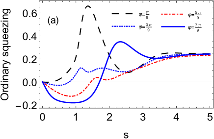
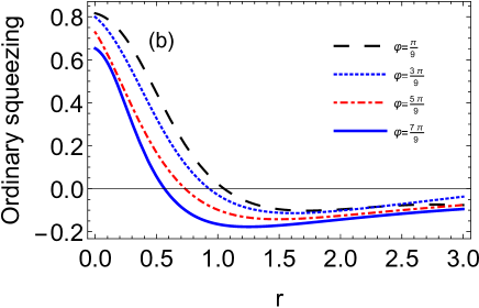
Figure 1: (Color online) The effects of postselected von Neumann measurement on ordinary squeezing of SPACS. Fig. 1(a) shows the quantity $S_{os}$as a function of coupling strength for different weak values with fixed coherent state parameter ($r=1$). Fig. 1(b) shows quantity $S_{os}$ as a function of coherent state parameter $r$ for different weak values with fixed coupling strength ($s=0.5$). Here, we take $\theta=\frac{\pi}{4}$, $\delta=\frac{\pi}{6}$.

Using the expression for $S_{os}$, the curves for this quantity are plotted, and the analytical results are shown in Fig. 1. In Fig. 1(a), we fixed the parameter $r=1$ and plot the $S_{os}$ as a function of coupling strength $s$ for different weak values quantified by $\varphi$. As we observed, when there is no interaction between system and poiner ($s=0$), there is no ordinary squeezing effect of initial SPACS at the $r=1$ point. However, in moderate coupling strength regions such as $0<s$<2 , the ordinary squeezing effect of SPACS is proportional to the weak value, i.e. the larger the weak value, the better its squeezing effect. From Fig. 1(a) we also can see that the ordinary squeezing effect of the light field gradually disappears and tends to the same value for different weak values with increasing coupling strength $s$ in the strong measurement regime. In Fig. 1(b), we plot $S_{os}$ as a function of the state parameter $r$ in the weak measurement regime by fixing the coupling strength $s$, i.g, $s=0.5$. It is very clear from the curves presented in Fig. 1 (b) that the ordinary squeezing effect of SPACS is increased when increasing the weak value, especially when $\varphi$ is taken as $\frac{7\pi}{9}$. Furthermore, along with the increasing $r$ (for $r$ values exceeding 1.5), the squeezing effect of the field for different weak values tended to be the same. According to von Neumann measurement theory, when the interaction strength is too large, the system is strongly measured and the size of the weak value has little impact on the squeezing effect.This statement can also be observed in Fig. 1(a) and (b). In the weak measurement regime the SPACS showed a good ordinary squeezing effect after postselected measurement with large weak values, and this can be seen as a result of the signal amplification feature of the weak measurement technique.

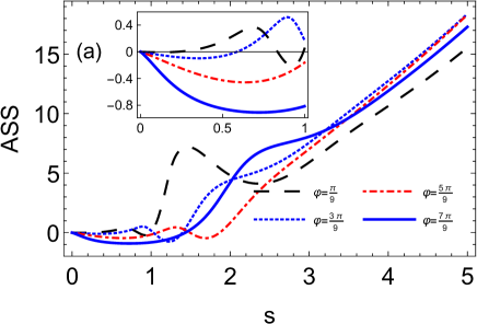
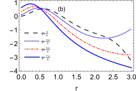
Figure 2: (Color online) The effects of postselected von Neumann measurement on ASS of SPACS. (a) the $S_{ass}$ as a function of coupling strength $s$ for different weak values with fixed coherent state parameter $r$ ($r=1$); (b) the $S_{ass}$ as a function of coherent state parameter $r$ for different weak values with fixed weak coupling strength $s$ ($s=0.5$). Other parameters are the same as those used in Fig. (1).

The quantity $S_{ass}$can characterize the ASS of SPACS if it takes negative values, and in Fig. 2 it is plotted as a function of various system parameters. As indicated in Fig. 2 (a), when we fixed the coherent state parameter $r$ ,the $S_{ass}$ can take negative values in the weak measurement regime ($s<1$) and its negativity increases when increasing the weak value quantified by $\varphi$. That is to say, in the weak measurement regime, the magnitude of the weak value has a linear relationship with the ASS effect of SPACS, i.g. The larger the weak value, the better the ASS effect. However, by increasing the coupling strength, the value of $S_{ass}$ became larger than zero and it indicates that there is no ASS effect on SPACS in the postselected strong measurement regime ($s>1$) no matter how large the value is taken. In order to further investigate the ASS of the radiation field in the weak measurement regime, we plot the $S_{ass}$ as a function of the coherent state parameter $r$ for different weak values with $s=0.5$. the analytical results are shown in Fig. 2b. We can see that when $r$ is relatively small, there is an ASS effect no matter how large the weak value becomes. By increasing the system parameter $r$, $S_{ass}$ takes negative values and its negativity is proportional to $r$. From Fig. 2a we can also observe that in the weak measurement regime, the weak values have positive effects on the ASS of SPACS, and it can also be considered a result of the weak signal amplification feature of the postselected weak measurement technique.

IV State distance and Wigner function

The postselected measurement taken on polarization degree of freedom of the beam could spoil the inherent properties presented in its spatial part. Before we investigate the phase-space distribution of SPACS after postselected von Neumanm measurement, we check the similarity between the initial SPACS $|\phi\rangle$ and the state $|\Phi\rangle$ after measurement. The state distance between those two states can be evaluated by

$$F=|\langle\phi|\Phi\rangle|^{2},$$ (23)

and its value is bounded $0\leq F\leq 1$. If $F=1$ ($F=0$), then the two states are totally same (totally different). The $F$ in our case can be calculated after substituting equations Eq. (3)and Eq. (8) into the Eq. (23), and the analytical results are shown in Fig. 3. In Fig. 3 we present the state distance $F$ as a function of system parameter $r$ for different coupling strengths with a fixed large weak value. As shown in Fig. 3, in the weak coupling regime ($s=0.5$), the state after the postselected measurement maintains similarity with the the coherent state parameter $r$. However, with increasing the measurement strength, the initial state $|\phi\rangle$ is spoiled and the similarity between the pointer states before and after the measurement is decreases.

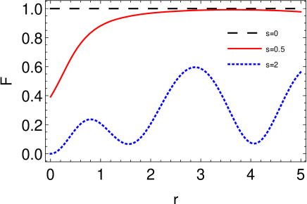
Figure 3: (Color online) The state distance between $|\Phi\rangle$ and initial SPACS $|\phi\rangle$ as a function of coherent state parameter $r$ for various coupling strengths. Here, we set values $\theta=\frac{\pi}{4}$, $\delta=\frac{\pi}{6}$, $\varphi=\frac{7\pi}{9}$.

In order to further explain the squeezing effects of SPACS after postselected von Neumann measurement, in the rest of this section we study the Wigner function of $|\Phi\rangle$. The Wigner distribution function is the closest quantum analogue of the classical distribution function in phase space. According to the value of the Wigner function we can intuitively determine the strength of its quantum nature, and the negative value of the Wigner function proves the nonclassicality of the quantum state. The Wigner function exists for any state, and it is defined as the two-dimensional Fourier transform of the symmetric order characteristic function. Thus, the Wigner function for the state $\rho=|\Phi\rangle\langle\Phi|$ is written as (Agarwal, 2013)

$$W(z)\equiv\frac{1}{\pi^{2}}\int_{-\infty}^{+\infty}\exp(\lambda^{\ast}z-\lambda z^{\ast})C_{W}(\lambda)d^{2}\lambda,$$ (24)

where $C_{N}(\lambda)$ is the normal ordered characteristic function,and is defined as

$$C_{W}(\lambda)=Tr\left[\rho e^{\lambda a^{\dagger}-\lambda^{\ast}a}\right].$$ (25)

Using the notation $\lambda^{\prime},$$\lambda^{\prime\prime}$ for the real and imaginary parts of $\lambda$ and setting $z=x+ip$ to emphasize the analogy between the radiation field quadratures and the normalized dimensionless position and momentum observables of the beam in phase space. We can rewrite the definition of the Wigner function in terms of $x,p$ and $\lambda^{\prime},\lambda^{\prime\prime}$ as

$$W(x,p)=\frac{1}{\pi^{2}}\int_{-\infty}^{+\infty}e^{2i(p\lambda^{\prime}-x\lambda^{\prime\prime})}C_{W}(\lambda)d\lambda^{\prime}d\lambda^{\prime\prime}.$$ (26)

By substituting the final normalized pointer state $|\Phi\rangle$ into Eq. (26), we can calculate the explicit expression of its Wigner function and it reads as

$$W(z) =\frac{2|\kappa|^{2}}{\pi(1+|\alpha|^{2})}e^{-2|z-\alpha|^{2}}\times$$

$$\{|1+\langle\sigma_{x}\rangle_{w}|^{2}w(\Gamma)+|1-\langle\sigma_{x}\rangle_{w}|^{2}w(-\Gamma)$$

$$\!\!\!\!\!\!\!\!\!+2\left(-1+|2z-\alpha|^{2}\right)Re[(1+\langle\sigma_{x}\rangle_{w})^{\ast}(1-\langle\sigma_{x}\rangle_{w})e^{2isIm[z]}]\}.$$ (27)

with

$$w(\Gamma) =e^{-\frac{1}{2}s^{2}}e^{-2(Re[\alpha]-Re[z])s}\times$$

$$\left(-1+|2z-\alpha|^{2}+2s(Re[\alpha]-2Re[z]+\frac{s}{2})\right)$$ (28)

This is a real Wigner function and its value is bounded $-\frac{2}{\pi}\leq W(\alpha)\leq\frac{2}{\pi}$ in whole phase space.

To depict the effects of the postselected von Neumann measurement on the non-classical feature of SPACS, in Fig. 4 we plot its curves for different parametric coherent state parameters $r$ and coupling strengths $s$. Each column from left to right in-turn indicate the different coherent state parameters $r$ for 0, 1 and 2, and each row from up to down represent the different coupling strengths $s$ for $0,0.5$ and $2$. It is observed that the positive peak of the Wigner function moves from the center to the edge position in phase space and its shape gradually becomes irregular with changing coupling strength $s$. From the first row (see Figs. 4a-c ) we can see that the original SPACS exhibit inherent features changing from single photon state to coherent states with gradually increasing coherent state parameter $r$. Figs. 4d-k indicate the phase space density function $W\left(z\right)$ after postselected von Neumann measurement. Fig. 4 d-f represent the Wigner function for fixed weak interaction strength $s=0.5.$ It can be observed that the Wigner function distribution shows squeezing in phase space compared to the original SPACS and this kind of squeezing is pronounced with increasing coupling strength (see Figs. 4g-k ). Furthermore, in Figs. 4(g-k) we can see that in the strong measurement regime significant interference structures manifest and the negative regions become larger than the initial pointer state.

As mentioned above, the existence of and progressively stronger negative regions of the Wigner function in phase space indicates the degree of nonclassicality of the associated state. From the above analysis we can conclude that after the postselected von Neumann measurement, the phase space distribution of SPACS is not only squeezed but the nonclassicality is also pronounced in the strong measurement regime.

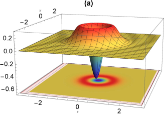
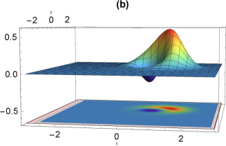
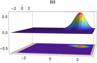
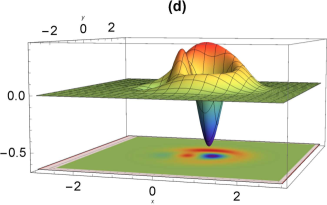
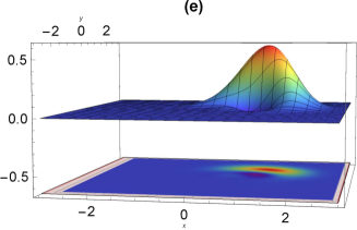
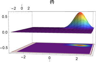
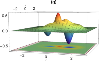
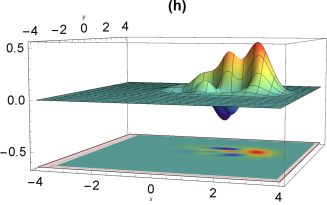
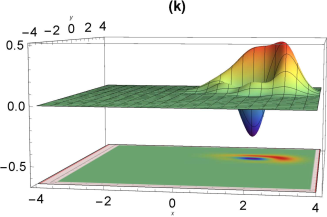
Figure 4: (Color online) Wigner function of SPACS with changing parameters. Each column is defined for the different coherent state parameter $\alpha$ with $r=0,1,2$, and are ordered accordingly from left to right. Figures (a) to (c) correspond to $s=0$, (d) to (f) correspond to $s=0.5$, and (g) to (k) correspond to $s=2$. Other parameters are the same as those used in Fig. (3).

V Conclusion

In this paper we have studied the squeezing and Wigner function of SPACS after postselected von Neumann measurement. In order to achieve our goal, we first determined the final state of the pointer state along with the standard measurement process. We examined the ordinary (first-order) and ASS effects after measurement, and found that in the weak measurement region, the ordinary squeezing and ASS of the light field increased significantly as the weak value increased.

To further explain our work, we examined the similarity between the initial SPACS and the state after measurement. We observed that under weak coupling, the state after the postselected measurement maintains similarity with the initial state. However, as the intensity of the measurement increases, the similarity between them gradually decreased and indicated that the measurement spoils the system state if the measurement is strong. We also investigate the Wigner function of the system after postselected measurement. It is observed that following the postselected von Neumann measurement, the phase space distribution of SPACS is not only squeezed, but also adevelops significant interference structures in the strongly measured regime. It also possess pronounced nonclassicality characterized with a large negative area in phase space.

We anticipate that the theoretical scheme in this paper may provide an effective method for solving practical problems in quantum information processing associated with SPACS.