NuSTAR monitoring of MAXI J1348-630: evidence of high density disc reflection

Abstract

We present the broadband spectral analysis of all the six hard, intermediate and soft state NuSTAR observations of the recently discovered transient black hole X-ray binary MAXI J1348-630 during its first outburst in 2019. We first model the data with a combination of a multi-colour disc and a relativistic blurred reflection, and, whenever needed, a distant reflection. We find that this simple model scheme is inadequate in explaining the spectra, resulting in a very high iron abundance. We, therefore, explore the possibility of reflection from a high-density disc. We use two different sets of models to describe the high-density disc reflection: relxill-based reflection models, and reflionx-based ones. The reflionx-based high-density disc reflection models bring down the iron abundance to around the solar value, while the density is found to be $10^{20.3-21.4}\rm cm^{-3}$. We also find evidence of a high-velocity outflow in the form of $\sim$7.3 keV absorption lines. The consistency between the best-fit parameters for different epochs and the statistical significance of the corresponding model indicates the existence of high-density disc reflection in MAXI J1348-630.

1 Introduction

Black hole X-ray binaries (BHBs) are systems with a black hole and a companion star. BHBs can be classified into persistent and transients based on the magnitude of flux change seen in them. In transient BHBs, the flux in the X-ray band can change by few orders of magnitude. The primary spectrum of BHBs can be modelled with a multi-temperature black body radiation emitted by an accretion disc (Novikov & Thorne, 1973; Shakura & Sunyaev, 1973), a Comptonisation (power-law) component due to the up-scattering of the soft disc photons in a high temperature compact structure called corona (Sunyaev & Titarchuk, 1980, 1985), and a reflection of the Comptonized photons off the top layer of the disc. The reflection features consist of iron emission lines at 6 to 7 keV along with a Compton hump at approximately 30-50 keV and an excess below 1 keV(Fabian, 2016), further smeared by the relativistic effects in the vicinity of the black hole. The relativistic reflection component provides insights on the disc-corona geometry (such as the size of the coronal region and the inner radius of the disc) and the changes of inner accretion processes throughout the evolution of BHB spectral states. Thus the BHB spectral states are characterised by the geometry of the disc and corona, and the interplay between the direct and reflection components. The main spectral states of transient BHBs are the low hard state (LHS) and the high soft state (HSS) (Belloni et al., 2000). The main conjecture is that in the HSS the disc extends until inner most circular orbit (ISCO), while the disc is truncated at a larger distance in the LHS (Esin et al., 1997; Belloni et al., 2000; Ponti et al., 2012a). While transiting between these states, they undergo a q-shaped hysteresis within the hardness intensity diagram (HID) (Fender et al., 2004; Remillard & McClintock, 2006). The source rises in intensity from the LHS before transiting into the HSS, and then falls in intensity before transiting back into the low hard state before vanishing into quiescence. Outflows in the form of jet and winds are also observed in these systems. A jet is generally seen in the hard state and stronger while the source transits from soft to hard state (Fender et al., 2004). Even though disc winds are stronger in the soft state in comparison to the hard state (Ponti et al., 2012b; Fukumura et al., 2021; Ratheesh et al., 2021), the state dependence of disc wind is not clearly understood.

A common outcome of reflection modelling of BHB X-ray spectra is super-solar iron abundance (Parker et al., 2015; Walton et al., 2016). This high iron abundance is a feature seen in AGN as well (e.g., Parker et al., 2018). Radiative levitation, or the enhancement of the metallicity due to radiation-pressure dominance of the inner disc, has been proposed as an explanation behind these super-solar abundances (Reynolds et al., 2012). While in some AGN, this kind of high metallicity could indeed be real (Wang et al., 2012), in most of the cases, this is perhaps an artefact of the model and the assumptions therein. An alternate explanation of the high iron abundances involves reflection off a high-density accretion disc. For most of the widely used disc reflection models, a constant electron density of ($n_{\rm e}=10^{15}\rm{cm^{-3}}$, inspired by the values observed in AGN) is assumed for the top layer of the disc, along with the assumption that the actual density does not have a significant effect on the predicted spectrum. While this density is appropriate for the very highest mass supermassive BHs in AGN (e.g., Grupe et al., 2010; Jiang et al., 2019b), BHBs may require higher densities (García et al., 2016). However, the free–free absorption and heating of the disc have both found to be quadratically dependent on density. As the density increases, the rise in free–free absorption leads to an increase in the temperature of the top layer of the disc, causing extra thermal emission and increasing the reflected emissions below 1 keV (Ross & Fabian, 2007; García et al., 2016). Thus, models taking into account this effect has been demonstrated to relieve the very high iron abundance required in other reflection models (e.g., Tomsick et al., 2018; Jiang et al., 2019b).

MAXI J1348-630 is such a transient BHB discovered by Gas Slit Camera (GSC) onboard Monitor of All-sky X-ray Image ($MAXI$) (Matsuoka et al., 2009), and classified as a BHB based on the estimated mass and spectral features (Tominaga et al., 2020). Previous studies, using $MAXI$/GSC, $Swift$/XRT (Tominaga et al., 2020) and $NICER$ data (Zhang et al., 2020), indicate that MAXI J1348-630 also exhibits a q-shaped hysteresis and that it is most likely a BHB. The source exhibited a hard to soft transition from MJD 58517 to MJD 58530 and returned back to the hard state around MJD 58600 (Tominaga et al., 2020). The distance to the source was estimated to be 3.39 kpc, based on the precise measurements using a dust scattering ring around the source (utilizing $SRG$/eROSITA and $XMM$-Newton data; Lamer et al. (2020)). Monitoring of the inner disc radius from the spectral analysis indicate a black hole mass of 11 $\pm$ 2 M_⊙ (Tominaga et al., 2020; Lamer et al., 2020). Even during the soft state the inner disc temperature was in the range of 0.5 to 0.7 keV (Tominaga et al., 2020; Zhang et al., 2020). The source underwent a failed outburst without hard to soft transition as also seen previously in some transients BHBs (Tominaga et al., 2020; Homan et al., 2013; Fürst et al., 2015; Stiele & Kong, 2020). The source showed type B quasi periodic oscillations (QPOs) during hard to soft transition generally accompanied by a relativistic jet (Belloni et al., 2020). The source was also detected in optical and ultraviolet (UV) and radio frequencies (Denisenko et al., 2019; Kennea & Negoro, 2019; Russell et al., 2019b; Russell et al., 2019a).

In this present investigation, we provide a broadband spectral view of MAXI J1348-630, observed with the Nuclear Spectroscopic Telescope Array (NuSTAR, (Harrison et al., 2013b)) during its first complete outburst during January-June, 2019. With its pile-up free performance, reasonably good energy resolution ($\sim$400 eV at 10 keV) and sensitivity, NuSTAR provides an opportunity to study the relativistic reflection features along with a well-constrained inner disc radius and inclination with great precision. We use all the 6 NuSTAR data (see table  1) during the first outburst of MAXI J1348-630, spanning the hard, intermediate and soft states, and model the spectra with different disc reflection models. In particular, we focus on the possibility of high density reflection. The paper is organised as follows. In section 2.2, we describe the data reduction procedure of NuSTAR, as well as the $MAXI$/GSC and Swift /BAT lightcurves and HID of MAXI J1348-630. We then present an in-depth spectral analysis of NuSTAR data in section  3.1, first with regular density disc reflection models and then with high density reflection models in section  3.1.1 and  3.1.2. Finally, we summarise our results and discuss their implications in section 4.

2 Observations and Data reduction

2.1 $MAXI$/GSC and Swift /BAT Lightcurve and HID

Since the BHBs evolve in timescales of the order of seconds to days, it is important to identify the state of the source based on continuous monitoring of the source. Daily monitoring of the X-ray sky have been possible due to the Neil Gehrels $Swift$ Observatory (Swift /BAT: Krimm et al., 2013) in the hard X-ray band and Gas Slit Camera on board Monitor of All-sky X-ray Image in the soft X-ray band (MAXI/GSC: Matsuoka et al., 2009). The daily averaged lightcurves of $Swift$/BAT and $MAXI$/GSC have been obtained from https://swift.gsfc.nasa.gov/results/transients/ and http://maxi.riken.jp. The top panel of Fig. 1 shows the $Swift$/BAT (grey) and $MAXI$/GSC (black) crab normalized lightcurves in 15-50 keV and 4-10 keV energy range, and the bottom panel shows the hardness ratio in 4-10 keV and 2-4 keV ranges. 1 Crab unit corresponds to 1.1 $\times$ 10^-8 ergs s^-1 cm^-2 and 9.2 $\times$ 10^-9 ergs s^-1 cm^-2 in the 4-10 keV and 2-4 keV energy bands covered by $MAXI$/GSC, and 1.3 $\times$ 10^-8 ergs s^-1 cm^-2 in the 15-50 keV energy band covered by Swift /BAT (Kirsch et al., 2005). The dotted lines indicate the start and stop of the hard to soft state transition obtained from Tominaga et al. (2020). The vertical coloured lines indicate the NuSTAR observations used in this analysis as outlined in the subsection below (also refer to table 1). Fig. 2, shows the hardness intensity diagram (HID). The soft and hard bands used for the hardness ratio is as same as the bottom panel of Fig. 1. The HID indicates that the source underwent a q-shaped hysteresis starting from the low hard state as generally seen in black hole X-ray binaries. The coloured points in the HID indicate the $MAXI$/GSC data on the days of the observations used in this work.

Instrument	Obs ID	Obs. date	Exposure (s)	Abbreviation	Epoch
		(yyyy-mm-dd)
NuSTAR	80402315002	2019-02-01	3038	Nu02 (maroon)	E1
NuSTAR	80402315004	2019-02-01	736	Nu04 (maroon)	E1
NuSTAR	80402315006	2019-02-06	4520	Nu06 (red)	E2
NuSTAR	80402315008	2019-02-11	4639	Nu08 (orange)	E3
NuSTAR	80402315010	2019-03-08	9714	Nu10 (cyan)	E4
NuSTAR	80402315012	2019-04-03	12490	Nu12 (darkblue)	E5

Table 1: NuSTAR observation details for MAXI J1348-630. We include only the observations considered in this work. The colours, mentioned within the brackets, indicate the corresponding observations in all the figures. The colours are in accordance with matplotlib colour palette.

2.2 NuSTAR

MAXI J1348-630 was observed with NuSTAR (Harrison et al., 2013a) 6 times in 5 different epochs during its first complete outburst cycle in January-June, 2019. The details of the NuSTAR observations and their colour coding followed throughout the rest of this work, are presented in table 1. From figure 2, it can be seen that the epoch E1 (maroon data point; comprised of the two contemporaneous NuSTAR observations Nu02 and Nu04, as denoted in table 1) is located in the hard state, while the epoch E2 (red; comprised of the NuSTAR observation Nu06) is situated at the hard-soft transition in the HID. The epochs E3-E5 (orange, cyan and darkblue points in figure 2) all belong to the soft state, with decreasing flux levels. The NuSTAR data are processed using v2.0.0 of the NuSTARDAS pipeline. We also use NuSTAR CALDB v20200813. A rip in the Multi Layer Insulation (MLI) at the exit aperture of the $NuSTAR$ Optics Module A (OMA), aligned with detector focal plane module FPMA, occurred presumably in early 2017. This has resulted in increased photon fluxes through OMA, resulting in low energy ($<$10 keV, more prominent in softer energies) excesses in FPMA spectra, as compared to FMPB. This effect of reduction in MLI covering fraction has been taken care of by implementing (through the numkarf module in NuSTARDAS v2.0.0, as well as the latest CALDB) time/temperature dependent correction to the FPMA effective area using specific on-axis ARF files (Madsen et al., 2020). However, there exist pathological observations in which this correction falls short. For these individual cases, the $NuSTAR$ SOC has provided an XSPEC multiplicative table model. We come across one such observation (Nu10/E4), and implement the suggested correction (see section 3.1). We filter background flares due to enhanced solar activity by setting saacalc = 2, saamode = OPTIMIZED, and tentacle = no in NUPIPELINE. Furthermore, due to the source being extremely bright, we used a modified value of the ’statusexpr’ keyword in NUPIPELINE, statusexpr=”STATUS==b0000xxx00xxxx000”, as suggested in the HEASARC NuSTAR analysis guide. The source spectra are extracted from circular regions of the radius 120${}^{{}^{\prime\prime}}$ centred on the source location. To avoid contamination by source photons from the extremely bright source regions, the background spectra are extracted from blank regions on the detector furthest from the source location. The spectra are grouped in $ISIS$ (Houck & Denicola, 2000) version 1.6.2-41 to have a signal-to-noise ratio of at least 25 per bin (15 in case of the fainter spectra in E5), to facilitate $\chi^{2}$ fitting statistics.

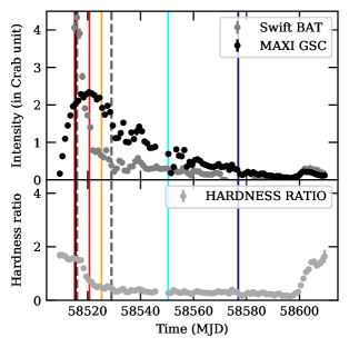
Figure 1: Top: $MAXI$/GSC (4-10 keV), $Swift$/BAT (15-50 keV) lightcurves are plotted in black and grey. Bottom: The corresponding hardness ratio (10-20 keV/4-10 keV) from $MAXI$/GSC. All the observations used in this analysis are marked by vertical colour shaded regions. The dotted lines indicate the start and stop of the hard to soft state transition.

Figure 2: The hardness intensity diagram (HID) for MAXI J1348-630. For the hardness ratio 4-10 keV and 2-4 keV energy band in $MAXI$/GSC is taken as hard and soft bands respectively (in grey). The coloured points indicate the $MAXI$/GSC data during the $NuSTAR$ observations used in this work.

3 Data Analysis and Results

The spectral fitting and statistical analysis are carried out using the XSPEC version v-12.11.0 (Arnaud, 1996). For the joint fitting between FPMA and FPMB, a cross-normalisation constant (implemented using Constant model in XSPEC) is allowed to vary freely for FPMB and is assumed to be unity for FPMA. To avoid the unexplained residuals below 4 keV in some of the observations, possibly related to the issue with the MLI blanketing as detailed in Madsen et al. (2020), an energy range between 4 keV and 79 keV is considered for the spectral fittings of all the epochs. To avoid the sharp instrumental features (as reported by Xu et al. (2018)), energies between 11-12 keV and 26-28 keV are excluded. All the models, as described below, include the Galactic absorption through the implementation of the TBabs model. The corresponding abundances are set in accordance with the Wilms et al. (2000) photoelectric cross-sections. The Galactic neutral hydrogen column density ($N_{\rm H}$) is fixed to $8.6\times 10^{21}\ \rm cm^{-2}$ (Tominaga et al., 2020) for all the described models. All parameter uncertainties are reported at the 90% confidence level for one parameter of interest. In addition to the $\chi^{2}$ and the degrees of freedom, we also provide the null hypothesis probability for each of the models we use. In order to facilitate comparisons between the different nested and non-nested models and to select better models, we also state the Akaike Information Criterion (AIC, Akaike, 1974) and Bayesian Information Criterion (BIC, Schwarz, 1978). AIC is more suitable to compare non-nested models, whereas BIC is more suited when nested models are compared (Kass & Raftery, 1995), although that is not a necessity. In general, BIC penalises models with higher number of free parameters more severely. The AIC is defined as:

$$\rm AIC=-2\ln\mathcal{L}+2k$$ (1)

where $\mathcal{L}$ is the likelihood of the best-fit model, $k$ is the number of free parameters. The BIC, on the other hand, is defined as:

$$\rm BIC=-2\ln\mathcal{L}+k\ln(N)$$ (2)

where $N$ is the total number of data points. The values of the $\chi^{2}$ for the best-fit models, $\chi^{2}_{\rm min}$, in our fits can be converted to likelihood by equating the two: $\chi^{2}_{\rm min}=-2\ln\mathcal{L}$. The values of AIC and BIC thus calculated for all our best-fit models, are provided in Tables  2, 3, 4 and  5. The model with the lowest AIC or BIC is the most preferred one. It should be noted, however, that the AIC and BIC compares models from pure statistical perspective; and one should also consider the physical interpretation of models and the reasonable range of their parameter values while selecting the ‘better’ model.

The spectra from all the epochs (E1 to E5) considered here are shown unfolded to a constant model in Figure  3 (left panel). A consistent spectral softening from hard to soft state can be observed. With our signal-to-noise ratio based binning, we find that the epochs E4 and E5 possess no statistically significant energy bins above 50 keV.

To highlight the spectral features more clearly, we plot the spectra from all the epochs as ratios to the best-fitting power-law model in Figure  3 (right panel). For the powerlaw fits, we only consider the energy intervals of 8-11 and 40-79 keV, where reflection from the disc has minimal effect. We then fit the 8-11,40-79 keV spectrum of each epoch with an absorbed cutoff power-law model, TBabs$\times$cutoffpl in XSPEC notation. Finally, we generate the 4-79 keV residuals by diving the data from each epoch with the corresponding absorbed cutoff power-law model. The resulting figure  3 shows a broad Fe K-$\alpha$ emission line peaking around 6.5 keV and a Compton hump at $\sim$20-40 keV for all the epochs, hinting the presence of relativistic reflection expected from an accretion disc extending close to a black hole (Fabian et al., 2000).

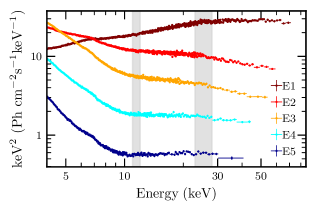
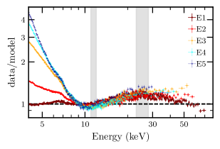
Figure 3: Left panel: NuSTAR spectra, unfolded with a constant model to see the spectral variations between the epochs. The colour coding for each epoch is detailed in table  1. Right panel: NuSTAR residuals, in form of data/model ratio, after a power-law fit. The soft excess, broad iron line and the Compton hump can be noticed. See section  3 for further details. The shaded grey region consists of energy bands ignored for detailed spectral fitting.

3.1 Quantitative modelling with reflection

For a detailed investigation of the broadband spectra including the reflection features, we start with the self-consistent relativistic disc reflection models from relxill model suite (relxill v1.3.10 : Dauser et al. (2014), García et al. (2014)). We assume an extended corona and use the model relxillCp which internally includes an thermal Comptonisation (Nthcomp: Zdziarski et al. (1996),Życki et al. (1999)) continuum. Due to the strong degeneracy between the inner radius ($R_{\rm in}$) of the accretion disc, and the dimensionless black hole spin parameter ($a$), we fit the data for $R_{\rm in}$ assuming a maximally spinning black hole ($a=0.998$). We fix the outer edge of the accretion disc ($R_{\rm out}$) at the maximum value for the model of $400R_{\rm g}$ (where $R_{\rm g}$ is the gravitational radius of the black hole, defined as $R_{\rm g}=GM/c^{2}$) and the emissivity indices at 3 ($q_{1}=q_{2}=3$). On the other hand, we keep the inclination angle free. To account for the narrow core of the Fe-K$\alpha$ line in the hard state data (Epoch E1), we use the unblurred reflection model xillverCp (García & Kallman, 2010). We use xillverCp only as a reflection component, freezing the refl_frac of xillverCp at -1, as only insignificant variations are found in the subsequent fits if the refl_frac is allowed to vary freely. We require an additional xillverCp for E3 as well. For both the cases, we assume the xillverCp component to be neutral to maintain simplicity. The electron temperatures ($T_{\rm e}$), spectral indices ($\Gamma$), iron abundances ($A_{\rm Fe}$) and inclinations ($\theta$), are assumed to be equal between the relxillCp and xillverCp components. To model the soft X-ray excess (as evident from Figure  3), we use the multicoloured disc black-body (diskbb: Mitsuda et al. (1984), Makishima et al. (1986)) model. As suggested by the instrument team, we also account for the MLI correction for FPMA in the pathological case of Nu10 (Epoch E4). This is done by the introduction of the multiplicative model nuMLIv1.mod suggested by NuSTAR SOC (Madsen et al., 2020), and fixing the MLI covering fraction of FPMA to the recommended value of 0.83.

After the continua of all the epochs are modelled, absorption features around 7.2-7.3 keV are observed in the residuals for all of the 5 epochs. This kind of absorption features in the Fe-K band are commonly associated with blueshifted FeXXV/FeXXVI lines, and are believed to arise from absorption by outflowing material launched from the accretion disc (e.g., Ponti et al., 2012a). The narrow absorption line complex cannot be properly resolved by $NuSTAR$, hence we model it simply using a Gaussian absorption line model (gabs in XSPEC).

This constitutes our model M1 in Table  2:

Nu02/04/08:
TBabs$\times$gabs$\times$(diskbb+relxillCp+xillverCp)

Nu06/10/12:
TBabs$\times$gabs$\times$(diskbb+relxillCp)

For epoch E1, the two NuSTAR observations (Nu02 and N04) are carried out within a short interval. For a consistent fit between the two observations, we allow the continuum parameters (Innermost temperature ($T_{\rm in}$) of the diskbb component, $T_{\rm e}$ and $\Gamma$ of the Nthcomp component in relxillCp) and all the normalisations to vary freely between them, tying up the absorption and reflection parameters ($R_{\rm in}$, $A_{\rm Fe}$, $\theta$ and ionisation parameter ($\xi$) of the relxillCp component) between the two observations.

From Table  2, we find that as the source moves from hard to soft states (E1 to E5), the $T_{\rm in}$ first increases before decreasing again, while the $T_{\rm e}$ increases before getting pegged at the parameter upper bound for relxillCp model. The disc is found to be highly ionised, and the inner edge of accretion disc is found to contract from $\sim 10R_{\rm g}$ to near the innermost stable circular orbit (ISCO). The inclination is found to be around 30-45 degrees.

However, there are some problems with the best-fit M1 model, as apparent from Table  2. First of all, the iron abundance of the disc is found to be significantly higher than solar, sometimes pegging at the upper limit of 10 times solar. This fact is further verified by performing a Markov chain Monte Carlo (MCMC) analysis with 50 walkers with chain lengths of 5000 for E2, E4 and E5. These values are most likely overestimated, given the ubiquity of apparent super-solar iron abundances (García et al., 2018). The overestimate has previously been attributed to high density discs (Svensson & Zdziarski, 1994; García et al., 2016) which would show stronger iron lines at a given metallicity (García et al., 2016; Tomsick et al., 2018). Secondly, this unusually high iron abundance is also found to be sometimes accompanied by systematically increasing residuals above 50 keV (see the uppermost panels showing the residuals in E3 and E4, in Figure  5). This feature has also been observed for Cyg X-1 by Tomsick et al. (2018). To address these issues, we subsequently explore the possibility of a high density disc by modeling all the NuSTAR spectra with high density reflection models.

3.1.1 relxill-based high density reflection models

To extend the disc density from its constant value of $n_{\rm e}=10^{15}cm^{-3}$ to higher values, we first use the relxill-based high density reflection model, relxillD. In this model, the continuum is assumed to be a power-law with a high energy cutoff (cutoffpl in XSPEC), with the cutoff energy ($E_{\rm cut}$) fixed at 300 keV. Instead, the disc density is treated as a free parameter, and can range from $10^{15}cm^{-3}$ to a maximum value of $10^{19}cm^{-3}$. In case of E1 and E3, similar to M1, we add a neutral distant reflection as the best-fit model. To make the model consistent, we use the cutoff power-law version of the distant reflection component, xillver. All the parameters are treated in a similar manner as M1. Thus our model M2 (see Table  3) becomes: Nu02/04/08:
TBabs$\times$gabs$\times$(diskbb+relxillD+xillver)

Nu06/10/12:
TBabs$\times$gabs$\times$(diskbb+relxillD)

From Table  3 it can be seen that for the same degrees of freedom, best-fit M2 provides $\Delta\chi^{2}$ of 18-23 less than M1 for most of the epochs. For the hard state observations in E1, the fit gets worse due to $kT_{\rm e}$ being fixed at a high value of 300 keV. The iron abundances, except in E4, are brought down to more reasonable values of 1.5-4 times solar. All the continuum and reflection parameters follow a similar trend as M1, and the presence of the absorption line is also noted. The densities are consistently found to be much higher than the relxillCp value of $10^{15}cm^{-3}$. Despite providing a better fit in general, we still face the problem of the disc densities pegging at the upper limit of $10^{19}cm^{-3}$ throughout E2 to E5.

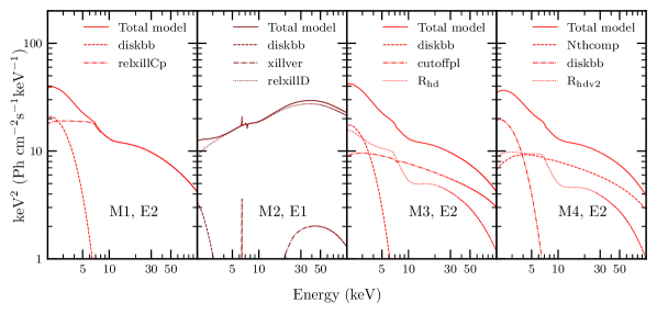
Figure 4: Best-fit models and model components for all the models (M1,M2,M3,M4), plotted for a representative epoch for each. The model corresponding model and epoch names are displayed in each panel. The bold, dashed, dotted and dash-dotted lines represent the total model, disc, relativistic blurred reflection and the unblurred distant reflection components, respectively. The epochs follow the colour coding from table  1. The spectral components are detailed in section  3.1,  3.1.1 and  3.1.2, and the implications discussed in section 4.

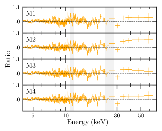
Figure 5: Residuals, in the form of data/model ratios, for each of the 4 models for two representative epochs E3 (orange, top panel) and E4 (cyan, bottom panel). For better visual representation, we display only the FPMA residuals. The light grey shaded regions indicate the 11.0-12.0 and 26.0-28.0 keV regions, ignored in this work due to unexplained systematics. See section 3.1 for model descriptions.

Figure 6: Residuals, in the form of data/model ratios, for different components of the best-fit model M4 for a representative epochs E2 (colour coded in accordance with table 1). For better visual representation, we display only the FPMA residuals. The panels, from top to bottom, demonstrate the improvement in residuals as further model components are added. $\rm R_{hdv2}$ abbreviates the reflection component, relconv$\otimes$reflionx_hd.The light grey shaded regions indicate the 11.0-12.0 and 26.0-28.0 keV regions, ignored in this work due to unexplained systematics. See section 3.1 for model descriptions.

3.1.2 reflionx-based high density reflection models

While relxillD-based model M2 provides a better fit than M1 and gives an indication of the presence of a high density disc, the disc density is found to peg at its upper limit of $10^{19}cm^{-3}$. To circumvent this issue, we switch from the relxill-based relxillD to reflionx-based (Ross & Fabian, 2005) high-density reflection model relflionx_hd, used by Tomsick et al. (2018) based on the code by Ross & Fabian (2007). relflionx_hd assumes a cutoff power-law continuum and provides only the reflection component. As opposed to relxillD, relflionx_hd has the disc density extending upto $10^{22}cm^{-3}$. While similar to relxillD, relflionx_hd has the cutoff energy fixed at 300 keV, in case of relflionx_hd the iron abundance is also fixed at the solar value ($A_{\rm Fe}=1$). We convolve the relflionx_hd component with smeared relativistic accretion disc line profiles using relconv (Dauser et al., 2010). Thus, for E2-E5, relconv*relflionx_hd forms the reflection component, while we use cutoffpl as the direct component. Similar to M2, we also use an additional xillver component as required for epoch E3, the cutoff energy of which we also fix at 300 keV. For the hard state spectra in E1, with low cutoff energy of $<$32 keV, the assumption of $E_{\rm cut}=300$ keV might pose an issue. To take care of this issue, we introduce an exponential cutoff model highecut to the reflection model, and use Nthcomp as the continuum. Following the procedure adapted by Pintore et al. (2015), we fix the $E_{{\rm cut}}$ and $E_{{\rm fold}}$ energies in the highecut model to the $kT_{{\rm e}}$ and $2.7\times kT_{{\rm e}}$ of the Nthcomp, respectively. Additionally, we use xillverCp to account for the narrow core of the Fe-K emission. Thus, our model M3 (best-fit parameters detailed in Table  4) becomes:

Nu02/04:
TBabs$\times$gabs$\times$(diskbb+Nthcomp+xillverCp+
(highecut$\times$relconv*reflionx_hd))

Nu08:
TBabs$\times$gabs$\times$(diskbb+cutoffpl+xillver+
(relconv*reflionx_hd))

Nu06/10/12:
TBabs$\times$gabs$\times$(diskbb+cutoffpl+(relconv*reflionx_hd))

It can be seen from Table  4 that M3 reduces the $\chi^{2}$ values as compared to M2, by values between 1 and 46 for E2-E5, depending on the epoch, and by a value of 92 for E1. This improvement over M2 for one less free parameter for E2-E5 and 4 additional free parameters for E1, results in an improvement of the goodness of the fits. The trends in the continuum as similar to before, with the value of $\Gamma$ for E1 being slightly harder than in M1 best-fit and $kT_{\rm e}$ attaining similar values. It is to be noted that the upper limit of the cutoffpl spectral index for relflionx_hd is 2.3. Thus, in case of E3 where the $\Gamma>2.3$, we fix the $\Gamma$ of the reflection component at 2.3 and allow the $\Gamma$ of the direct cutoffpl component to vary freely. The disc density is found to be much higher than $10^{19}cm^{-3}$, with values ranging in $0.7-27\times 10^{20}cm^{-3}$. However, both the disc density and the ionization parameter are found to vary quite significantly between the observations. This could be an artefact of the modeling.

Although M3 provides a superior fit than M2, relflionx_hd still has a few limitations. Due to the cutoff energy being fixed at 300 keV, the hard state spectra cannot be consistently modeled with relflionx_hd. Furthermore, due to the upper limit of spectral index being fixed at 2.3, we are unable to constrain the value properly for E3. Finally, another crucial limitation of relflionx_hd is that the iron abundance is fixed at the solar value. Super-solar metallicity are quite common in X-ray binaries and are sometimes thought to be caused by radiative levitation (Reynolds et al., 2012).

For more flexible modelling, we use a more recent, Nthcomp continuum-based high density reflection model reflionx_hdv2 (John Tomsick, private communication). Here, the electron temperature and the iron abundance are free parameters, along with the other parameters present in reflionx_hd. Thus, our model M4 (see Table  5) becomes:

Nu02/04/08:
TBabs$\times$gabs$\times$(diskbb+Nthcomp+xillverCp+
(relconv*reflionx_hdv2))

Nu06/10/12:
TBabs$\times$gabs$\times$(diskbb+Nthcomp+(relconv*reflionx_hdv2))

From Table  5, it can be seen that, statistically, M4 provides almost the same quality of fit as M3. The change in $\chi^{2}$ is minimal, ranging from 1 to 10 for 2 degrees of freedom (1 degree of freedom in case of E1), even though the null hypothesis probability improves. In fact, the AIC and BIC actually increases for E4, while for E3 and E5 they are almost the same. However, as discussed in the beginning of section  3, we have to take into account the consistency of parameter values and their physical interpretation before selecting the optimal model. For M4, the values of $kT_{\rm in}$ and $\Gamma$ are found to be broadly consistent between M4 and M3. Furthermore, the $kT_{\rm e}$ increases monotonically with time from $\sim 32-37$ keV to the the maximum value of 400 keV from E1 to E5, while the $R_{\rm in}$ decreases from $\sim 13R_{\rm g}$ $\sim 2.6R_{\rm g}$. Apart from E1 (for which the null hypothesis probability is still quite low), all the other inclinations are found to be consistent around 30-38 degrees. As in the case of M3, M4 also shows variations in $\xi$, although the variation is minimal between E2,E3 and E5. Furthermore, the iron abundances are also found to be consistent, hovering around the solar value. Apart form E4, the disc density are constrained to $\sim 10^{20.3-20.7}cm^{-3}$ and are found to be consistent between all the epochs. The normalisations of the reflionx_hdv2 components are found to monotonically decrease between E1 and E5. Finally, the absorption feature around 7.3 keV is found to be prominent and consistent across the epochs. For this consistency and the minimal statistical improvement, we can generally consider M4 as the most appropriate model. It can be observed, however, that for epoch E4, the density assumes a much higher value than the other observations or even compared to best-fit M3 model for E4. M4 also results in a slightly higher BIC and AIC for E4. Thus, even though M3 and M4 are almost equivalent for E4, M3 can as well be considered a more consistent model for E4.

The models M1-M4, along with the individual components, are presented for a few representative epochs in Figure  4. The data/model ratios for all the models (M1-M4) are presented for the epochs E3 and E4 in Figure  5. The improvement in the fit residuals with the addition of different model components for the best-fit model M4, is presented for a representative epoch E2 in Figure 6.

4 Discussions and Conclusions

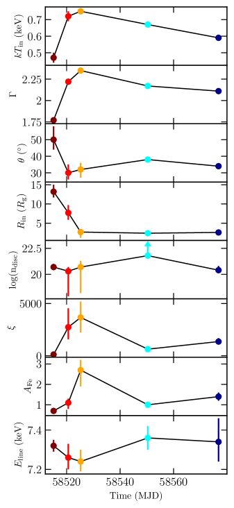
Figure 7: Time evolution of best-fit parameters for the best-fit model M4. The model is described in section  3.1.2, and the parameters are detailed in table  5. The data points are plotted for the different epochs following the colour scheme detailed in table  1.

In this work, we present a consistent NuSTAR spectral analysis of the recently discovered BHB MAXI J1348-630, for 5 different epochs spanning hard, hard-soft transition and soft states during its first complete outburst in 2019. We model the NuSTAR spectra with the combination of a multi-coloured disc blackbody component, a Comptonisation continuum and relxill-based relativistic reflection components. The resulting model, M1 (see section  3.1 and table  2) proves quite inadequate to account for all the spectral features. Extremely high iron abundances, hints of high energy excess and low values of null hypothesis probabilities are found. There are a few scenarios that can explain the overabundance and the occasional high energy excesses. Presence of a jet, specially in the hard state, could explain some of the extreme parameters (Nowak et al., 2011). A jet has indeed been observed for MAXI J1348-630 by Carotenuto et al. (2021). However, jet models have more free parameters, a comprehensive study of which is beyond our current work. One may try to approximate the presence of jet with the addition of an excess power-law or broken power-law component. However, this approach is found to lead to no further improvement for MAXI J1348-630. Alternately, presence of a second Comptonization region (Yamada et al., 2013; Basak et al., 2017; Chakraborty et al., 2020) has been proposed as the emission mechanism for MAXI J1348-630 (García et al., 2021). However, addition of a second corona component did not result in any significant improvement in our results. The third scenario, as investigated for other BHBs by Tomsick et al. (2018); Jiang et al. (2019a), could be high density reflection. In our current work, we explore this scenario in detail for MAXI J1348-630.

In section  3.1.1, we explore the high density ($n_{\rm e}>10^{15}\rm cm^{-3}$) reflection in MAXI J1348-630 using the relxill-based relxillD model. The resulting model, M2 (best-fit parameters detailed in table  3), is found to yield statistically better fits. While M2 mostly resolves the issue with iron overabundance, the density is found to get pegged at the upper limit ($n_{\rm e}=10^{19}\rm cm^{-3}$) of the model. Moreover, due to the electron temperature being fixed at 300 keV, relxillD is found to be inadequate for the hard state epoch E1. To better constrain the density, we then use the reflionx-based high density reflection models (see section  3.1.2). The resulting models, M3 and M4 (tables  4 and  5 details the best-fit parameter values), generate fits with AIC and BIC less than M1 or M2. The cutoffpl continuum-based reflionx_hd is limited by the facts that the iron abundance and the electron temperatures are fixed at the solar value and 300 keV, respectively. The latest, Nthcomp continuum-based model reflionx_hdv2 alleviates these limitations. Although both M3 and M4 result in similar qualities of fits from a statistical point of view, M4 has more consistent parametrisation across the epochs. M3, however, results in a more consistent density value for the epoch E4, and a more consistent inclination for E1. The best-fit parameters for the most appropriate models (tables  4 and  5), are found to follow the following evolution (figure  7):

• The temperature of the innermost part of the accretion disc ($kT_{\rm in}$) first increases to a maximum value of $\sim$0.75 keV around the epoch E3, and then decreases. This trend exactly follows that found by Tominaga et al. (2020) and Zhang et al. (2020). The temporal evolution of $\Gamma$ is also found to be similar to $kT_{\rm in}$.

• The truncation radius of the inner accretion disc gets consistently closer to the black hole as the spectral state progresses from hard to soft state.

• The corona temperature increases from $\sim$32-37 keV to a high value (pegged at the default maximal value of 400 keV for Nthcomp) as the state goes from hard to soft.

• The inclination, apart from the hard state, is consistent between the observations. The low null hypothesis probability suggests that M4 may not be the most suitable model for hard state epoch E1. For all the other observations, the inclination is found to be $\sim$30-40 degrees.

• The disc densities are more or less constant at $\sim 10^{(20.3-21.4)}\rm cm^{-3}$. This kind of high disc density has previously been found in other BHBs (e.g., Tomsick et al., 2018; Jiang et al., 2019a).

• The abundances are found to be close to the solar value. This is in stark contrast with the relxill-based M1 model.

All these values are further supported by the MCMC analysis (appendix  A). This consistency of the different parameters and steady improvement in reduced $\chi^{2}$ for the high-density reflection models, gives further credence to our conclusion. García et al. (2016), however, emphasizes that the atomic physics underneath the the reflection models is only known to be accurate up to densities of $\rm\sim 10^{19}cm^{-3}$. Hence, more accurate determinations of the rates of atomic transitions and other quantities can have an impact on the high-density reflection models, thereby affecting our results.

As opposed to the relxillD, our relconv$\otimes$reflionx_hd implementation is not fully self-consistent. In case of a real, extended accretion disc, the density should depend on the distance from the central compact object (Svensson & Zdziarski, 1994). However, the reflionx_hd model assumes an optically thick, slab-like atmosphere of a constant density (Ross & Fabian, 2005). Thus, in our implementation, the X-rays are assumed to be reflected from a single layer at a single photoionization radius ($R_{\rm ion}$, Mori et al. (2019)). Therefore, following Mori et al. (2019), we perform a sanity check for the self-consistency of best-fit M4 model parameters. Assuming an isotropically emitting illuminating source (the corona), the ionisation parameter in reflionx_hd model can be redefined as $\xi=\frac{L}{nR_{\rm ion}^{2}}$ (where $L$ is the illuminating luminosity, $n$ is the hydrogen number density). Now, the electron density($n_{\rm e}$) quoted by reflionx_hd can be equated to the disc density ($n_{disc}$), as the accretion disc is believed to be primarily composed of hydrogen (this assumption has been followed throughout this work). Furthermore, we can use the 0.1-200 keV unabsorbed luminosity from the Comptonization and the reflection components (thus, disregarding the diskbb) as a proxy for the illuminating luminosity $L$. This is found to be $\sim 1\times 10^{37}-3\times 10^{38}$ ergs/s, depending on the epoch in consideration. Thus, using the values of $n_{\rm disc}$ and $\xi$ from table  5, we can calculate $R_{\rm ion}$ as:

$$R_{\rm ion}=\sqrt{\frac{L^{\rm comp+refl}_{\rm 0.1-200\ keV}}{n_{\rm disc}\times\xi}}$$ (3)

On the other hand, we can utilize the inner radius of the accretion disc $R_{\rm in}$ as quoted by the relconv model from table  5. Therefore, assuming that the corona is located directly above the central black hole, $R_{\rm ion}\gtrsim R_{\rm in}$ can be imposed as a necessary self-consistency condition. Using the values from table  5, we find that for all our observations, this condition is satisfied within error bars.

The mass of MAXI J1348-630 has been reported to be $9.1^{+1.6}_{-1.2}\ M_{\odot}$ by Jana et al. (2020) and $13\pm 2\ M_{\odot}$ by Tominaga et al. (2020), further rectified to be $11\pm 2\ M_{\odot}$ by Lamer et al. (2020). Using equation 3 from Wang et al. (2018) and the correction factor from Kubota et al. (1998) for the soft state diskbb normalisation, we find the black hole mass to be $\sim 11.6-19.4\ M_{\odot}$. We note that the calculated mass from the NuSTAR diskbb normalisation is likely to be incorrect, due to lack of $<$3 keV spectra in NuSTAR. Even though a simultaneous Swift -XRT or NICER data could be used to estimate the mass more accurately, we leave such a hard+soft X-ray spectral modelling for this source for a future work. For now, we use the black hole mass and distance estimates from Lamer et al. (2020). Using the Model M4, we find the integrated unabsorbed 0.1-200 keV luminosity of MAXI J1348-630 to be $1.3\times 10^{38},1.2\times 10^{38},1.4\times 10^{38},6.6\times 10^{37}$ and $3.3\times 10^{37}$ erg/s, for E1, E2, E3, E4 and E5, respectively. This implies that From E1 to E5, MAXI J1348-630 was accreting at $6-24\%$ of the Eddington luminosity ($L_{\rm Edd}$). Using the solution for radiation pressure-dominated disc from Svensson & Zdziarski (1994) (equation 1 in García et al., 2016), we can then explain the consistency of density between E1,E2 and E3, and the increase of density for E4. For a radiation-pressure dominated $\alpha$-disc at high accretion rate ($\dot{m}$ much larger than 0.1), $n_{\rm e}\propto\dot{m}^{-2}$. Assuming an accretion efficiency $\epsilon$ to be 20$\%$ (Novikov & Thorne, 1973; Agol & Krolik, 2000), $\dot{m}=\rm L_{X}/\epsilon L_{Edd}\approx L_{0.1-200\ keV}/\epsilon L_{Edd}$. Using this relation, we find an inverse relation between the X-ray luminosity $L_{\rm X}$ and the disc density. Therefore, for E1, E2 and E3 (where the 0.1-200 keV luminosity is found to be roughly the same), the disc density remains constant. The disc density then increases for E4, where the 0.1-200 keV luminosity decreases by a factor of 2. However, this does not explain the consistency between the densities derived for E5 and that of E1, E2 and E3.

Finally, another significant highlight of our work is the detection of absorption feature at $\sim$7.3 keV throughout the epochs. Accounting for this feature, either using the multiplicative Gaussian absorption profile gabs or by using a Gaussian emission line profile with negative normalisation, improves the fit by $\Delta\chi^{2}\sim 26-166$ (for 3 fewer degrees of freedom), indicating that the absorption feature is significantly detected. The lines are thus found to have equivalent widths (in absolute value) of $\sim$10-20 eV. This kind of absorption lines are indication of outflows in the form of ionised accretion disc winds, believed to be ubiquitous in X-ray binaries (e.g., Ponti et al., 2012a) and important to the accretion process (Begelman et al., 1983). Disc winds in BHBs are generally known to have an equatorial geometry (e.g., Ponti et al., 2012a). However, recent evidences (Chiang et al., 2012; Xu et al., 2020; Wang et al., 2021) hint towards the existence of ultrafast winds even in non-equatorial directions. Among the prevalent driving mechanisms proposed, the thermally driven winds prefer high inclinations (Tomaru et al., 2020), while the MHD-driven winds can flow out at all directions (Fukumura et al., 2017). Therefore, the discovery of such a low-inclination ultrafast outflow as MAXI J1348-630, hints towards a magnetic origin (Chakraborty et al., in prep).

To summarise, we have characterised the broadband X-ray spectra of the recently-discovered transient black hole X-ray binary MAXI J1348-630 through systematic investigation of all the NuSTAR data during its first complete outburst in 2019. We find consistent continuum and reflection parameters, and the existence of an ultrafast outflow. We also find, using different relxill and reflionx-based reflection models, a significant evidence of reflection off a high density disc.

Table 2: Parameters of NuSTAR fits to MAXI J1348-630 spectra with model M1. The model M1 is detailed in section 3.1. Errors represent 90% confidence intervals.

Spectral Component	Parameter	Epoch
		E1	E2	E3	E4	E5
diskbb	$kT_{\mathrm{in}}$ (keV)	$0.48_{-0.07}^{+0.04}$ (Nu02)	$0.69_{-0.02}^{+0.02}$	$0.80_{-0.01}^{+0.01}$	$0.69_{-0.01}^{+0.01}$	$0.59_{-0.01}^{+0.01}$
		$0.47_{-0.08}^{+0.07}$ (Nu04)	…	…	…	…
	norm $(\times 10^{4})$	$1.1_{-0.4}^{+1.0}$ (Nu02)	$1.9_{-0.3}^{+0.4}$	$1.8_{-0.1}^{+0.1}$	$1.7_{-0.1}^{+0.1}$	$1.9_{-0.1}^{+0.2}$
		$1.2_{-1.1}^{+0.5}$ (Nu04)	…	…	…	…
relxillCp	$\Gamma$	$1.70_{-0.01}^{+0.01}$ (Nu02)	$2.22_{-0.01}^{+0.01}$	$2.36_{-0.01}^{+0.01}$	$2.18_{-0.01}^{+0.01}$	$2.09_{-0.02}^{+0.05}$
		$1.70_{-0.01}^{+0.01}$ (Nu04)	…	…	…	…
	$kT_{\mathrm{e}}$ (keV)	$31_{-3}^{+2}$ (Nu02)	$184_{-34}^{+97}$	$>201$	$>282$	$>178$
		$28_{-2}^{+2}$ (Nu04)	…	…	…	…
	$\theta$ (∘)	$42_{-4}^{+4}$	$37_{-2}^{+2}$	$42_{-1}^{+1}$	$35_{-2}^{+2}$	$31_{-2}^{+2}$
	$R_{\mathrm{in}}$ ($R_{\mathrm{g}}$)	$10.0_{-4.0}^{+2.7}$	$<2.7$	$2.4_{-0.2}^{+0.2}$	$2.9_{-1.3}^{+1.6}$	$<3.2$
	$\log{\xi}$ (log[erg cm/s])	$3.40_{-0.10}^{+0.08}$	$4.44_{-0.07}^{+0.06}$	$4.00_{-0.08}^{+0.05}$	$4.22_{-0.06}^{+0.08}$	$4.05_{-0.15}^{+0.05}$
	$A_{\rm Fe}$ ($A_{\rm Fe,\odot}$)	$1.4_{-0.4}^{+0.5}$	$>5.3$	$4.1_{-0.3}^{+0.4}$	$>9.6$	$>6.8$
	$\mathcal{R}$	$0.09$	$0.18$	$0.19$	$0.28$	$0.52$
	norm	$0.18$ (Nu02)	$0.19$	$0.13$	$0.03$	$0.06$
		$0.17$ (Nu04)	…	…	…	…
xillverCp	norm $(\times 10^{-2})$	$1.0$ (Nu02)	…	$0.6$	…	…
		$0.7$ (Nu04)	…	…	…	…
gabs	$E_{\mathrm{line}}$ (keV)	$7.26_{-0.09}^{+0.07}$	$7.21_{-0.05}^{+0.04}$	$7.16_{-0.03}^{+0.04}$	$7.26_{-0.12}^{+0.18}$	$7.19_{-0.14}^{+0.11}$
	$\sigma_{\mathrm{line}}$ (keV)	$0.14_{-0.09}^{+0.08}$	$0.11_{-0.04}^{+0.05}$	$<0.2$	$<0.2$	$<0.2$
	line depth $(\times 10^{-2})$	$1.24$	$1.16$	$1.63$	$2.83$	$0.84$
$\chi^{2}/{\rm d.o.f.}$		$2255/2029$	$1182/1036$	$884/804$	$784/722$	$721/714$
null hypothesis probability		$2.6\times 10^{-4}$	$1.0\times 10^{-3}$	$2.6\times 10^{-2}$	$5.3\times 10^{-2}$	$4.2\times 10^{-1}$
AIC		$2303.3$	$1209.9$	$917.6$	$812.5$	$749.0$
BIC		$2438.3$	$1279.3$	$997.6$	$876.9$	$813.2$
	$C_{\mathrm{FPMB}}$	$1.03$	$1.02$	$1.02$	$1.01$	$1.00$
Unabsorbed flux	3.0–70.0 keV	$1.13\times 10^{-7}$ (Nu02)	$7.49\times 10^{-8}$	$5.59\times 10^{-8}$	$2.0\times 10^{-8}$	$6.6\times 10^{-9}$
	($\rm erg/cm^{2}/s$)	$1.13\times 10^{-7}$ (Nu04)	…	…	…	…

Note: $T_{\mathrm{in}}$: Temperature of the inner disc; norm: Normalisation of the corresponding spectral parameter; $\Gamma$: Asymptotic power-law photon index; $T_{\mathrm{e}}$: Electron temperature of the corona, determining the high energy rollover; $\theta$: Inclination of the inner disc; $R_{\mathrm{in}}$: Inner disc radius (in units of $R_{\mathrm{\rm g}}$); $\xi$: Ionisation parameter of the accretion disc, defined as $\xi=L/nR^{2}$, with L, n, R being the ionising luminosity, gas density and the distance to the ionised source, respectively; $A_{\rm Fe}$: Iron abundance, in the units of solar abundance; $\mathcal{R}$: Reflection fraction; $E_{\rm line}$: The central line energy for the Gaussian absorption model; $\sigma_{\rm line}$: line width of the absorption line; $C_{\mathrm{FPMB}}$: the flux normalisation constant for FPMB (determined by multiplicative ‘constant’ parameter in the spectral models), estimated with respect to the FPMA flux.

Table 3: Parameters of NuSTAR fits to MAXI J1348-630 spectra with model M2. The model M2 is detailed in section 3.1.1. Errors represent 90% confidence intervals.

Spectral Component	Parameter	Epoch
		E1	E2	E3	E4	E5
diskbb	$kT_{\mathrm{in}}$ (keV)	$0.41_{-0.04}^{+0.04}$ (Nu02)	$0.65_{-0.02}^{+0.02}$	$0.75_{-0.01}^{+0.01}$	$0.68_{-0.01}^{+0.01}$	$0.60_{-0.01}^{+0.01}$
		$0.37_{-0.06}^{+0.07}$ (Nu04)	…	…	…	…
	norm $(\times 10^{4})$	$4.2_{-1.9}^{+4.9}$ (Nu02)	$2.4_{-0.4}^{+0.5}$	$2.6_{-0.2}^{+0.2}$	$1.9_{-0.1}^{+0.1}$	$1.8_{-0.1}^{+0.1}$
		$10.6_{-11.9}^{+9.7}$ (Nu04)	…	…	…	…
relxillD	$\Gamma$	$1.55_{-0.01}^{+0.01}$ (Nu02)	$2.21_{-0.01}^{+0.03}$	$2.28_{-0.01}^{+0.01}$	$2.16_{-0.01}^{+0.01}$	$2.11_{-0.02}^{+0.02}$
		$1.55_{-0.01}^{+0.01}$ (Nu04)	…	…	…	…
	$\theta$ (∘)	$23_{-3}^{+3}$	$36_{-1}^{+2}$	$24_{-1}^{+2}$	$26_{-3}^{+2}$	$31_{-2}^{+1}$
	$R_{\mathrm{in}}$ ($R_{\mathrm{g}}$)	$9.3_{-1.2}^{+1.5}$	$<4.2$	$2.7_{-0.3}^{+0.4}$	$3.1_{-0.5}^{+0.5}$	$<3.4$
	$\log{\xi}$ (log[erg cm/s])	$3.82_{-0.02}^{+0.01}$	$4.09_{-0.06}^{+0.13}$	$4.05_{-0.10}^{+0.09}$	$4.02_{-0.09}^{+0.14}$	$3.40_{-0.17}^{+0.09}$
	$A_{\rm Fe}$ ($A_{\rm Fe,\odot}$)	$1.6_{-0.1}^{+0.1}$	$4.0_{-0.9}^{+0.9}$	$3.4_{-0.4}^{+0.4}$	$>6.2$	$3.8_{-0.9}^{+1.5}$
	$\log{n_{\rm disc}}$ (log[$\rm cm^{-3}$])	$17.8_{-0.5}^{+0.2}$	$>17.9$	$>18.5$	$>18.8$	$>18.8$
	$\mathcal{R}$	$0.40$	$0.37$	$0.79$	$0.28$	$0.42$
	norm	$0.12$ (Nu02)	$0.16$	$0.06$	$0.03$	$0.01$
		$0.12$ (Nu04)	…	…	…	…
xillver	norm $(\times 10^{-2})$	$2.0$ (Nu02)	…	$0.5$	…	…
		$1.8$ (Nu04)	…	…	…	…
gabs	$E_{\mathrm{line}}$ (keV)	$7.40_{-0.41}^{+0.07}$	$7.27_{-0.05}^{+0.04}$	$7.12_{-0.05}^{+0.04}$	$7.29_{-0.04}^{+0.04}$	$7.16_{-0.05}^{+0.27}$
	$\sigma_{\mathrm{line}}$ (keV)	$<0.2$	$0.17_{-0.06}^{+0.05}$	$<0.2$	$0.15_{-0.05}^{+0.07}$	$<0.2$
	line depth $(\times 10^{-2})$	$0.93$	$1.53$	$1.3$	$1.80$	$0.63$
$\chi^{2}/{\rm d.o.f.}$		$2348/2030$	$1164/1036$	$861/804$	$761/722$	$722/714$
null hypothesis probability		$1.1\times 10^{-5}$	$3.3\times 10^{-3}$	$7.9\times 10^{-2}$	$1.5\times 10^{-1}$	$4.1\times 10^{-1}$
AIC		$2356.4$	$1192.0$	$895.4$	$789.2$	$749.9$
BIC		$2485.9$	$1261.4$	$975.5$	$853.6$	$814.2$
	$C_{\mathrm{FPMB}}$	$1.03$	$1.02$	$1.02$	$1.00$	$1.00$
Unabsorbed flux	3.0–70.0 keV	$1.13\times 10^{-7}$ (Nu02)	$7.51\times 10^{-8}$	$5.64\times 10^{-8}$	$2.0\times 10^{-8}$	$6.65\times 10^{-9}$
	($\rm erg/cm^{2}/s$)	$1.14\times 10^{-7}$ (Nu04)	…	…	…	…

Note: $T_{\mathrm{in}}$: Temperature of the inner disc; norm: Normalisation of the corresponding spectral parameter; $\Gamma$: Asymptotic power-law photon index; $\theta$: Inclination of the inner disc; $R_{\mathrm{in}}$: Inner disc radius (in units of $R_{\mathrm{\rm g}}$); $\xi$: Ionisation parameter of the accretion disc, defined as $\xi=L/nR^{2}$, with L, n, R being the ionising luminosity, gas density and the distance to the ionised source, respectively; $A_{\rm Fe}$: Iron abundance, in the units of solar abundance; $n_{\rm disc}$: density of the top layer of the accretion disc, assumed to be equal to the corresponding electron number density; $\mathcal{R}$: Reflection fraction; $E_{\rm line}$: The central line energy for the Gaussian absorption model; $\sigma_{\rm line}$: line width of the absorption line; $C_{\mathrm{FPMB}}$: the flux normalisation constant for FPMB (determined by multiplicative ‘constant’ parameter in the spectral models), estimated with respect to the FPMA flux.

Table 4: Parameters of NuSTAR fits to MAXI J1348-630 spectra with model M3. The model M3 is detailed in section 3.1.2. Errors represent 90% confidence intervals.

Spectral Component	Parameter	Epoch
		E1	E2	E3	E4	E5
diskbb	$kT_{\mathrm{in}}$ (keV)	$0.47_{-0.20}^{+0.09}$ (Nu02)	$0.69_{-0.02}^{+0.02}$	$0.76_{-0.01}^{+0.01}$	$0.67_{-0.02}^{+0.02}$	$0.60_{-0.02}^{+0.01}$
		$0.43_{-0.08}^{+0.09}$ (Nu04)	…	…	…	…
	norm $(\times 10^{4})$	$0.9_{-0.2}^{+8.1}$ (Nu02)	$1.5_{-0.6}^{+0.9}$	$2.1_{-0.1}^{+0.1}$	$2.0_{-0.3}^{+0.4}$	$1.8_{-0.3}^{+0.4}$
		$1.5_{-0.7}^{+5.1}$ (Nu04)	…	…	…	…
Nthcomp	$\Gamma$	$1.74_{-0.01}^{+0.01}$ (Nu02)	…	…	…	…
		$1.74_{-0.01}^{+0.01}$ (Nu04)	…	…	…	…
	$kT_{\mathrm{e}}$ (keV)	$31_{-1}^{+1}$ (Nu02)	…	…	…	…
		$29_{-1}^{+1}$ (Nu04)	…	…	…	…
cutoffpl	$\Gamma$	…	$2.23_{-0.01}^{+0.02}$	$2.40_{-0.02}^{+0.02}$*	$2.15_{-0.03}^{+0.02}$	$2.09_{-0.05}^{+0.05}$
relconv	$\theta$ (∘)	$34_{-1}^{+1}$	$38_{-3}^{+2}$	$30_{-12}^{+4}$	$35_{-4}^{+4}$	$35_{-4}^{+4}$
	$R_{\mathrm{in}}$ ($R_{\mathrm{g}}$)	$8.6_{-1.4}^{+1.6}$	$<5.0$	$3.0_{-0.5}^{+0.4}$	$2.5_{-0.1}^{+0.1}$	$<3.2$
reflionx_hd	$\xi$ (erg cm/s)	$167_{-51}^{+60}$	$3652_{-1002}^{+545}$	$1608_{-395}^{+663}$	$796_{-202}^{+398}$	$1301_{-816}^{+842}$
	$n_{\rm disc}$ ($\rm\times 10^{20}cm^{-3}$)	$10.7_{-7.7}^{+24.7}$	$0.7_{-0.3}^{+0.7}$	$9.2_{-2.7}^{+3.2}$	$27.1_{-14.5}^{+26.1}$	$3.3_{-1.9}^{+7.5}$
	norm	$60$ (Nu02)	$214$	$66$	$14$	$7.4$
		$55$ (Nu04)	…	…	…	…
xillver(Cp)	norm $(\times 10^{-2})$	$0.2$ (Nu02)	…	$1.8$	…	…
		$0.2$ (Nu04)	…	…	…	…
gabs	$E_{\mathrm{line}}$ (keV)	$7.00_{-0.05}^{+0.04}$	$7.36_{-0.05}^{+0.05}$	$7.27_{-0.06}^{+0.07}$	$7.39_{-0.05}^{+0.05}$	$7.38_{-0.12}^{+0.15}$
	$\sigma_{\mathrm{line}}$ (keV)	$0.27_{-0.03}^{+0.04}$	$0.26_{-0.06}^{+0.06}$	$0.13_{-0.08}^{+0.09}$	$0.25_{-0.08}^{+0.08}$	$0.26_{-0.11}^{+0.14}$
	line depth $(\times 10^{-2})$	$3.1$	$2.4$	$1.1$	$3.9$	$3.3$
$\chi^{2}/{\rm d.o.f.}$		$2256/2026$	$1154/1037$	$815/805$	$756/723$	$720/715$
null hypothesis probability		$2.3\times 10^{-4}$	$6.4\times 10^{-3}$	$4.0\times 10^{-1}$	$1.9\times 10^{-1}$	$4.4\times 10^{-1}$
AIC		$2304.5$	$1179.8$	$846.9$	$781.9$	$746.0$
BIC		$2439.6$	$1244.2$	$922.2$	$841.7$	$805.7$
	$C_{\mathrm{FPMB}}$	$1.03$	$1.02$	$1.02$	$1.01$	$1.00$
Unabsorbed flux	3.0–70.0 keV	$1.13\times 10^{-7}$ (Nu02)	$7.5\times 10^{-8}$	$5.6\times 10^{-8}$	$2.0\times 10^{-8}$	$6.7\times 10^{-9}$
	($\rm erg/cm^{2}/s$)	$1.13\times 10^{-7}$ (Nu04)	…	…	…	…

Note: $T_{\mathrm{in}}$: Temperature of the inner disc; norm: Normalisation of the corresponding spectral parameter; $\Gamma$: Asymptotic power-law photon index; $\theta$: Inclination of the inner disc; $R_{\mathrm{in}}$: Inner disc radius (in units of $R_{\mathrm{\rm g}}$); $\xi$: Ionisation parameter of the accretion disc, defined as $\xi=L/nR^{2}$, with L, n, R being the ionising luminosity, gas density and the distance to the ionised source, respectively; $n_{\rm disc}$: density of the top layer of the accretion disc, assumed to be equal to the corresponding electron number density; $E_{\rm line}$: The central line energy for the Gaussian absorption model; $\sigma_{\rm line}$: line width of the absorption line; $C_{\mathrm{FPMB}}$: the flux normalisation constant for FPMB (determined by multiplicative ‘constant’ parameter in the spectral models), estimated with respect to the FPMA flux.

Table 5: Parameters of NuSTAR fits to MAXI J1348-630 spectra with model M4. The model M4 is detailed in section 3.1.2. Errors represent 90% confidence intervals.

Spectral Component	Parameter	Epoch
		E1	E2	E3	E4	E5
diskbb	$kT_{\mathrm{in}}$ (keV)	$0.47_{-0.03}^{+0.03}$ (Nu02)	$0.72_{-0.03}^{+0.03}$	$0.75_{-0.01}^{+0.01}$	$0.67_{-0.01}^{+0.01}$	$0.59_{-0.01}^{+0.01}$
		$0.46_{-0.02}^{+0.03}$ (Nu04)	…	…	…	…
	norm $(\times 10^{4})$	$0.3_{-0.2}^{+0.5}$ (Nu02)	$1.4_{-0.2}^{+0.2}$	$2.5_{-0.1}^{+0.2}$	$2.0_{-0.2}^{+0.2}$	$2.0_{-0.1}^{+0.2}$
		$0.3_{-0.2}^{+1.5}$ (Nu04)	…	…	…	…
Nthcomp	$\Gamma$	$1.77_{-0.01}^{+0.01}$ (Nu02)	$2.22_{-0.03}^{+0.03}$	$2.35_{-0.03}^{+0.03}$	$2.17_{-0.02}^{+0.01}$	$2.11_{-0.01}^{+0.02}$
		$1.76_{-0.01}^{+0.01}$ (Nu04)	…	…	…	…
	$kT_{\mathrm{e}}$ (keV)	$37_{-1}^{+1}$ (Nu02)	$142_{-26}^{+94}$	$>10$	$>169$	$>175$
		$32_{-1}^{+2}$ (Nu04)	…	…	…	…
relconv	$\theta$ (∘)	$50_{-6}^{+8}$	$30_{-4}^{+5}$	$32_{-5}^{+4}$	$38_{-1}^{+1}$	$34_{-1}^{+1}$
	$R_{\mathrm{in}}$ ($R_{\mathrm{g}}$)	$13.2_{-1.5}^{+1.8}$	$7.7_{-1.8}^{+2.0}$	$2.7_{-1.5}^{+0.5}$	$2.4_{-0.4}^{+0.6}$	$2.6_{-0.3}^{+0.3}$
reflionx_hdv2	$\xi$ (erg cm/s)	$120_{-6}^{+6}$	$2736_{-1159}^{+1811}$	$3664_{-1435}^{+1527}$	$632_{-208}^{+184}$	$1358_{-280}^{+320}$
	$A_{\rm Fe}$ ($A_{\rm Fe,\odot}$)	$0.7_{-0.1}^{+0.1}$	$1.1_{-0.3}^{+0.2}$	$2.7_{-0.8}^{+0.5}$	$1.0_{-0.1}^{+0.1}$	$1.4_{-0.2}^{+0.2}$
	$\log{n_{\rm disc}}$ (log[$\rm cm^{-3}$])	$20.7_{-0.3}^{+0.3}$	$20.3_{-2.4}^{+0.4}$	$20.7_{-2.5}^{+0.6}$	$>21.8$	$20.4_{-0.2}^{+0.4}$
	norm	$66$ (Nu02)	$27$	$15$	$3.6$	$3.1$
		$64$ (Nu04)	…	…	…	…
xillverCp	norm $(\times 10^{-2})$	$1.3$ (Nu02)	…	$0.8$	…	…
		$0.7$ (Nu04)	…	…	…	…
gabs	$E_{\mathrm{line}}$ (keV)	$7.32_{-0.03}^{+0.03}$	$7.26_{-0.06}^{+0.07}$	$7.24_{-0.05}^{+0.06}$	$7.36_{-0.06}^{+0.06}$	$7.34_{-0.10}^{+0.12}$
	$\sigma_{\mathrm{line}}$ (keV)	$0.26_{-0.03}^{+0.04}$	$0.22_{-0.08}^{+0.07}$	$0.13_{-0.01}^{+0.07}$	$0.23_{-0.06}^{+0.06}$	$0.22_{-0.09}^{+0.13}$
	line depth $(\times 10^{-2})$	$2.9$	$1.6$	$1.2$	$3.5$	$1.9$
$\chi^{2}/{\rm d.o.f.}$		$2245/2025$	$1144/1035$	$810/803$	$757/721$	$719/713$
null hypothesis probability		$4.0\times 10^{-4}$	$1.0\times 10^{-2}$	$4.2\times 10^{-1}$	$1.7\times 10^{-1}$	$4.3\times 10^{-1}$
AIC		$2295.3$	$1173.6$	$846.3$	$786.9$	$748.6$
BIC		$2435.9$	$1248.0$	$931.0$	$855.9$	$817.4$
	$C_{\mathrm{FPMB}}$	$1.03$	$1.03$	$1.03$	$1.02$	$1.00$
Unabsorbed flux	3.0–70.0 keV	$1.13\times 10^{-7}$(Nu02)	$7.5\times 10^{-8}$	$5.6\times 10^{-8}$	$2.0\times 10^{-8}$	$6.7\times 10^{-9}$
	($\rm erg/cm^{2}/s$)	$1.13\times 10^{-7}$ (Nu04)	…	…	…	…

Note: $T_{\mathrm{in}}$: Temperature of the inner disc; norm: Normalisation of the corresponding spectral parameter; $\Gamma$: Asymptotic power-law photon index; $\theta$: Inclination of the inner disc; $R_{\mathrm{in}}$: Inner disc radius (in units of $R_{\mathrm{\rm g}}$); $\xi$: Ionisation parameter of the accretion disc, defined as $\xi=L/nR^{2}$, with L, n, R being the ionising luminosity, gas density and the distance to the ionised source, respectively; $A_{\rm Fe}$: Iron abundance, in the units of solar abundance; $n_{\rm disc}$: density of the top layer of the accretion disc, assumed to be equal to the corresponding electron number density; $E_{\rm line}$: The central line energy for the Gaussian absorption model; $\sigma_{\rm line}$: line width of the absorption line; $C_{\mathrm{FPMB}}$: the flux normalisation constant for FPMB (determined by multiplicative ‘constant’ parameter in the spectral models), estimated with respect to the FPMA flux.

Data Availability

The observational data used in this paper are publicly available at NASA’s High Energy Astrophysics Science Archive Research Center (HEASARC; https://heasarc.gsfc.nasa.gov/). All the spectral figures are generated using the python implementation (pyxspec) of XSPEC. The MCMC results are plotted using the cornner.py module (Foreman-Mackey, 2016). Any additional information will be available upon reasonable request.

Appendix A MCMC results

To estimate better errorbars for some of the most important quantities for out model M4, we perform a Markov chain Monte Carlo (MCMC) analysis by using the XSPEC implementation of the EMCEE code (xspec_emcee), written by Jeremy Sanders. We use the Goodman–Weare algorithm, with 50 walkers, chain lengths of 5000, and burn-in lengths of 500. The results of the MCMC are plotted in figures  8, 9, 10, 11 and  12. The contours denote the 1,2 and 3-$\sigma$ confidence contours for the 2D posterior distributions, while the value and errors quoted are the mean and 68% confidence levels for the 1D posterior distributions. The values are consistent with our spectral fits and gives further credence to our results.

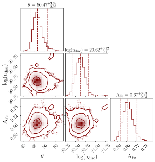
Figure 8: MCMC results for the epoch E1 and best-fit model M4.

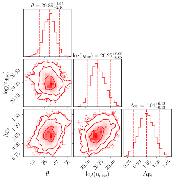
Figure 9: MCMC results for the epoch E2 and best-fit model M4.

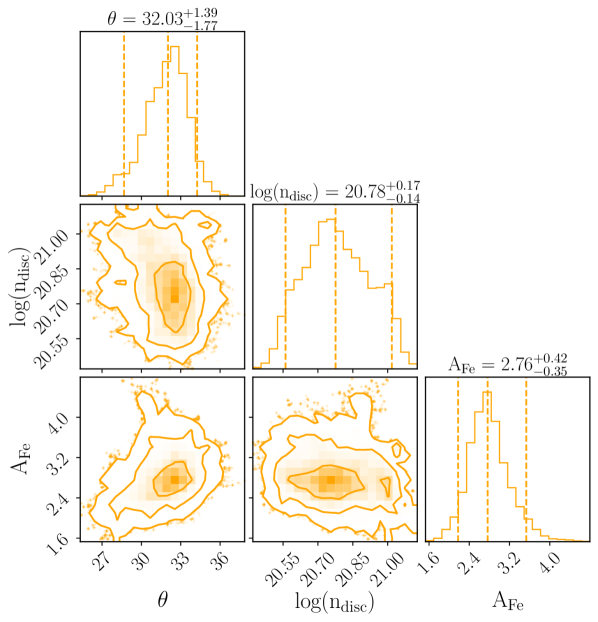
Figure 10: MCMC results for the epoch E3 and best-fit model M4.

Figure 11: MCMC results for the epoch E4 and best-fit model M4.

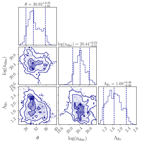
Figure 12: MCMC results for the epoch E5 and best-fit model M4.

References

- Agol & Krolik (2000) Agol E., Krolik J. H., 2000, ApJ, 528, 161
- Akaike (1974) Akaike H., 1974, IEEE Transactions on Automatic Control, 19, 716
- Arnaud (1996) Arnaud K. A., 1996, in Jacoby G. H., Barnes J., eds, Astronomical Society of the Pacific Conference Series Vol. 101, Astronomical Data Analysis Software and Systems V. p. 17
- Basak et al. (2017) Basak R., Zdziarski A. A., Parker M., Islam N., 2017, MNRAS, 472, 4220
- Begelman et al. (1983) Begelman M. C., McKee C. F., Shields G. A., 1983, ApJ, 271, 70
- Belloni et al. (2000) Belloni T., Klein-Wolt M., Méndez M., van der Klis M., van Paradijs J., 2000, A&A, 355, 271
- Belloni et al. (2020) Belloni T. M., Zhang L., Kylafis N. D., Reig P., Altamirano D., 2020, Monthly Notices of the Royal Astronomical Society, 496, 4366–4371
- Carotenuto et al. (2021) Carotenuto F., et al., 2021, arXiv e-prints, p. arXiv:2103.12190
- Chakraborty et al. (2020) Chakraborty S., Navale N., Ratheesh A., Bhattacharyya S., 2020, MNRAS, 498, 5873
- Chiang et al. (2012) Chiang C.-Y., Reis R. C., Walton D. J., Fabian A. C., 2012, MNRAS, 425, 2436
- Dauser et al. (2010) Dauser T., Wilms J., Reynolds C. S., Brenneman L. W., 2010, MNRAS, 409, 1534
- Dauser et al. (2014) Dauser T., Garcia J., Parker M. L., Fabian A. C., Wilms J., 2014, MNRAS, 444, L100
- Denisenko et al. (2019) Denisenko D., et al., 2019, The Astronomer’s Telegram, 12430, 1
- Esin et al. (1997) Esin A. A., McClintock J. E., Narayan R., 1997, ApJ, 489, 865
- Fabian (2016) Fabian A. C., 2016, Astronomische Nachrichten, 337, 375
- Fabian et al. (2000) Fabian A. C., Iwasawa K., Reynolds C. S., Young A. J., 2000, PASP, 112, 1145
- Fender et al. (2004) Fender R. P., Belloni T. M., Gallo E., 2004, Monthly Notices of the Royal Astronomical Society, 355, 1105–1118
- Foreman-Mackey (2016) Foreman-Mackey D., 2016, The Journal of Open Source Software, 1, 24
- Fukumura et al. (2017) Fukumura K., Kazanas D., Shrader C., Behar E., Tombesi F., Contopoulos I., 2017, Nature Astronomy, 1, 0062
- Fukumura et al. (2021) Fukumura K., Kazanas D., Shrader C., Tombesi F., Kalapotharakos C., Behar E., 2021, arXiv e-prints, p. arXiv:2103.05891
- Fürst et al. (2015) Fürst F., et al., 2015, ApJ, 808, 122
- García & Kallman (2010) García J., Kallman T. R., 2010, ApJ, 718, 695
- García et al. (2014) García J., et al., 2014, ApJ, 782, 76
- García et al. (2016) García J. A., Fabian A. C., Kallman T. R., Dauser T., Parker M. L., McClintock J. E., Steiner J. F., Wilms J., 2016, MNRAS, 462, 751
- García et al. (2018) García J. A., Kallman T. R., Bautista M., Mendoza C., Deprince J., Palmeri P., Quinet P., 2018, in Workshop on Astrophysical Opacities. p. 282 (arXiv:1805.00581)
- García et al. (2021) García F., Méndez M., Karpouzas K., Belloni T., Zhang L., Altamirano D., 2021, MNRAS, 501, 3173
- Grupe et al. (2010) Grupe D., Komossa S., Leighly K. M., Page K. L., 2010, ApJS, 187, 64
- Harrison et al. (2013a) Harrison F. A., et al., 2013a, ApJ, 770, 103
- Harrison et al. (2013b) Harrison F. A., et al., 2013b, ApJ, 770, 103
- Homan et al. (2013) Homan J., Fridriksson J. K., Jonker P. G., Russell D. M., Gallo E., Kuulkers E., Rea N., Altamirano D., 2013, ApJ, 775, 9
- Houck & Denicola (2000) Houck J. C., Denicola L. A., 2000, in Manset N., Veillet C., Crabtree D., eds, Astronomical Society of the Pacific Conference Series Vol. 216, Astronomical Data Analysis Software and Systems IX. p. 591
- Jana et al. (2020) Jana A., Debnath D., Chatterjee D., Chatterjee K., Chakrabarti S. K., Naik S., Bhowmick R., Kumari N., 2020, ApJ, 897, 3
- Jiang et al. (2019a) Jiang J., Fabian A. C., Wang J., Walton D. J., García J. A., Parker M. L., Steiner J. F., Tomsick J. A., 2019a, MNRAS, 484, 1972
- Jiang et al. (2019b) Jiang J., et al., 2019b, MNRAS, 489, 3436
- Kass & Raftery (1995) Kass R. E., Raftery A. E., 1995, Journal of the American Statistical Association, 90, 773
- Kennea & Negoro (2019) Kennea J. A., Negoro H., 2019, The Astronomer’s Telegram, 12434, 1
- Kirsch et al. (2005) Kirsch M. G., et al., 2005, in Siegmund O. H. W., ed., Society of Photo-Optical Instrumentation Engineers (SPIE) Conference Series Vol. 5898, UV, X-Ray, and Gamma-Ray Space Instrumentation for Astronomy XIV. pp 22–33 (arXiv:astro-ph/0508235), doi:10.1117/12.616893
- Krimm et al. (2013) Krimm H. A., et al., 2013, ApJS, 209, 14
- Kubota et al. (1998) Kubota A., Tanaka Y., Makishima K., Ueda Y., Dotani T., Inoue H., Yamaoka K., 1998, PASJ, 50, 667
- Lamer et al. (2020) Lamer G., Schwope A. D., Predehl P., Traulsen I., Wilms J., Freyberg M., 2020, arXiv e-prints, p. arXiv:2012.11754
- Madsen et al. (2020) Madsen K. K., Grefenstette B. W., Pike S., Miyasaka H., Brightman M., Forster K., Harrison F. A., 2020, arXiv e-prints, p. arXiv:2005.00569
- Makishima et al. (1986) Makishima K., Maejima Y., Mitsuda K., Bradt H. V., Remillard R. A., Tuohy I. R., Hoshi R., Nakagawa M., 1986, ApJ, 308, 635
- Matsuoka et al. (2009) Matsuoka M., et al., 2009, PASJ, 61, 999
- Mitsuda et al. (1984) Mitsuda K., et al., 1984, PASJ, 36, 741
- Mori et al. (2019) Mori K., et al., 2019, ApJ, 885, 142
- Novikov & Thorne (1973) Novikov I. D., Thorne K. S., 1973, in Black Holes (Les Astres Occlus). pp 343–450
- Nowak et al. (2011) Nowak M. A., et al., 2011, ApJ, 728, 13
- Parker et al. (2015) Parker M. L., et al., 2015, ApJ, 808, 9
- Parker et al. (2018) Parker M. L., Miller J. M., Fabian A. C., 2018, MNRAS, 474, 1538
- Pintore et al. (2015) Pintore F., et al., 2015, MNRAS, 450, 2016
- Ponti et al. (2012a) Ponti G., Fender R. P., Begelman M. C., Dunn R. J. H., Neilsen J., Coriat M., 2012a, MNRAS, 422, L11
- Ponti et al. (2012b) Ponti G., Fender R. P., Begelman M. C., Dunn R. J. H., Neilsen J., Coriat M., 2012b, MNRAS, 422, L11
- Ratheesh et al. (2021) Ratheesh A., Tombesi F., Fukumura K., Soffitta P., Costa E., Kazanas D., 2021, A&A, 646, A154
- Remillard & McClintock (2006) Remillard R. A., McClintock J. E., 2006, ARA&A, 44, 49
- Reynolds et al. (2012) Reynolds C. S., Brenneman L. W., Lohfink A. M., Trippe M. L., Miller J. M., Fabian A. C., Nowak M. A., 2012, ApJ, 755, 88
- Ross & Fabian (2005) Ross R. R., Fabian A. C., 2005, MNRAS, 358, 211
- Ross & Fabian (2007) Ross R. R., Fabian A. C., 2007, MNRAS, 381, 1697
- Russell et al. (2019a) Russell T., Anderson G., Miller-Jones J., Degenaar N., Eijnden J. v. d., Sivakoff G. R., Tetarenko A., 2019a, The Astronomer’s Telegram, 12456, 1
- Russell et al. (2019b) Russell D. M., Al Yazeedi A., Bramich D. M., Baglio M. C., Lewis F., 2019b, The Astronomer’s Telegram, 12829, 1
- Schwarz (1978) Schwarz G., 1978, Annals of Statistics, 6, 461
- Shakura & Sunyaev (1973) Shakura N. I., Sunyaev R. A., 1973, A&A, 500, 33
- Stiele & Kong (2020) Stiele H., Kong A. K. H., 2020, ApJ, 889, 142
- Sunyaev & Titarchuk (1980) Sunyaev R. A., Titarchuk L. G., 1980, A&A, 500, 167
- Sunyaev & Titarchuk (1985) Sunyaev R. A., Titarchuk L. G., 1985, A&A, 143, 374
- Svensson & Zdziarski (1994) Svensson R., Zdziarski A. A., 1994, ApJ, 436, 599
- Tomaru et al. (2020) Tomaru R., Done C., Ohsuga K., Odaka H., Takahashi T., 2020, MNRAS, 494, 3413
- Tominaga et al. (2020) Tominaga M., et al., 2020, ApJ, 899, L20
- Tomsick et al. (2018) Tomsick J. A., et al., 2018, ApJ, 855, 3
- Walton et al. (2016) Walton D. J., et al., 2016, ApJ, 826, 87
- Wang et al. (2012) Wang H., Zhou H., Yuan W., Wang T., 2012, ApJ, 751, L23
- Wang et al. (2018) Wang Y., Méndez M., Altamirano D., Court J., Beri A., Cheng Z., 2018, MNRAS, 478, 4837
- Wang et al. (2021) Wang Y., et al., 2021, ApJ, 906, 11
- Wilms et al. (2000) Wilms J., Allen A., McCray R., 2000, ApJ, 542, 914
- Xu et al. (2018) Xu Y., et al., 2018, ApJ, 852, L34
- Xu et al. (2020) Xu Y., Harrison F. A., Tomsick J. A., Walton D. J., Barret D., García J. A., Hare J., Parker M. L., 2020, ApJ, 893, 30
- Yamada et al. (2013) Yamada S., Makishima K., Done C., Torii S., Noda H., Sakurai S., 2013, PASJ, 65, 80
- Zdziarski et al. (1996) Zdziarski A. A., Johnson W. N., Magdziarz P., 1996, MNRAS, 283, 193
- Zhang et al. (2020) Zhang L., et al., 2020, MNRAS, 499, 851
- Życki et al. (1999) Życki P. T., Done C., Smith D. A., 1999, MNRAS, 309, 561