Relaxed Zero-Forcing Beamformer under Temporally-Correlated Interference

Abstract

The relaxed zero-forcing (RZF) beamformer is a quadratically-and-linearly constrained minimum variance beamformer. The central question addressed in this paper is whether RZF performs better than the widely-used minimum variance distortionless response and zero-forcing beamformers under temporally-correlated interference. First, RZF is rederived by imposing an ellipsoidal constraint that bounds the amount of interference leakage for mitigating the intrinsic gap between the output variance and the mean squared error (MSE) which stems from the temporal correlations. Second, an analysis of RZF is presented for the single-interference case, showing how the MSE is affected by the spatio-temporal correlations between the desired and interfering sources as well as by the signal and noise powers. Third, numerical studies are presented for the multiple-interference case, showing the remarkable advantages of RZF in its basic performance as well as in its application to brain activity reconstruction from EEG data. The analytical and experimental results clarify that the RZF beamformer gives near-optimal performance in some situations.

organization=Department of Electronics and Electrical Engineering, Keio University,addressline=Hiyoshi 3-14-1, Kohoku-ku, city=Yokohama, postcode=223-8522, country=JAPAN

organization=Interdisciplinary Center for Modern Technologies and the Faculty of Physics, Astronomy and Informatics, Nicolaus Copernicus University,city=Torun, country=POLAND

1 Introduction

Beamforming is an attractive technology to filter out those interfering (or jamming) signals which are spatially apart from the signal of interest. It has a long history (see e.g., [1]) and has been applied to a wide range of applications including radar, sonar, wireless communications, acoustics, electroencephalography (EEG), among many others. For the upcoming fifth generation (5G) wireless network and Internet of things (IoT) technologies, for instance, beamforming is considered as a key component to revolutionize connectivity as well as massive MIMO (multiple input multiple output) and millimeter wave [2, 3, 4]. The minimum-variance distortionless response (MVDR) beamformer minimizes the variance of the beamformer output under a linear constraint to preserve the desired signal undistorted [5]. The MVDR beamformer is known to achieve the optimal performance among all linear beamformers in the absence of correlations among sources. In many applications, however, the sources have temporal correlation, which makes MVDR no longer optimal [6]. Throughout the paper, unless otherwise stated explicitly, the term “correlation” means a temporal correlation between the desired and interfering sources. The zero-forcing (ZF) beamformer (aka. the nulling beamformer) [7, 6, 8, 9] minimizes the output variance under multiple linear constraints to preserve the desired signal undistorted and, at the same time, to nullify the interfering signals. Although it could attain better performance than MVDR in the correlated-source settings with high signal to noise ratio (SNR), its performance becomes even worse than MVDR in low SNR cases as it amplifies the noise [8]. The MVDR and ZF beamformers are particular examples of the linearly constrained minimum variance (LCMV) beamformer [10, 5], and can be implemented by efficient adaptive algorithms such as the constrained normalized least mean square (CNLMS) algorithm [11].

The studies of the temporal correlation between the desired and interfering signals date back at least to 1970’s [12] in the communication area. The major causes of the correlation are multipath propagation which may also happen in other applications such as acoustics) and/or “smart” jammers which aim to transmit antiphase replicas of the desired signal for jamming the transmission. In the worst case, the desired and interfering signals would be coherent; i.e., one source signal is an amplitude-scaled phase-shifted version of another one, or in other words the correlation coefficient has a unit amplitude. To alleviate this problem, spatial smoothing and its improved versions have been proposed, and the impacts of the correlation coefficient on the performance have been investigated in the literature (see [1, Section 6.12] and the references therein). This technique, however, has several limitations. For instance, it is only applicable to a regular array geometry such as uniform linear arrays, and/or it requires twice as many sensors as signal sources. An efficient beamformer design that can manage the correlated interference would be beneficial in the future wireless network systems to enhance the connectivity.

Another primary application of beamformers is in inverse problems in EEG and magnetoencephalography (MEG), which are imaging modalities that provide a direct measure of the brain activity by measuring the voltage with a set of sensors placed at various locations on the scalp of the subject. The EEG inverse problem aims to localize and reconstruct the sources of brain electrical activity from the EEG measurements. It is widely known that neighboring brain activities (sources) have strong correlations typically, and the signal correlation still remains a challenging issue to be addressed in the brain signal processing area. Focusing on EEG, this is especially true for applications requiring online processing of beamformer output such as brain-computer interface (BCI) [13, 14] and source-space EEG neurofeedback, which is currently another hot topic in brain signal processing [15, 16]. To date, the dominant beamforming technique used in these fields has been the MVDR beamformer, see, e.g., [17, 18, 19]. Therefore, an introduction of a beamformer design which suppresses efficiently interfering activity, includes as special cases the MVDR and ZF beamformers, and is amenable to efficient adaptive implementation, should bring significant benefits to BCI and source-space EEG neurofeedback.

Let us now turn our attention to the relaxed zero forcing (RZF) beamformer [20, 21]. Despite its close link to the ZF beamformer, RZF has solely been studied under the assumption that the source signals are mutually uncorrelated in time domain. In this case, MVDR is the optimal linear beamformer, and hence no other linear beamformer can outperform it. In fact, the key point of the previous works of RZF lies in its adaptive implementation. The central theme addressed therein is an efficient use of the side information about the interference channel for enhancing the convergence speed of adaptive algorithms. The side information is accommodated in the RZF formulation as an ellipsoidal constraint that bounds the contribution of interference in the output using the interference channel information. The RZF beamformer contains MVDR and ZF as its two extremes: MVDR does not consider the correlation explicitly, while ZF annihilates the interfering signals completely. The RZF beamformer belongs to the class of linearly and quadratically constrained minimum variance (LQCMV) beamformer due to the presence of the quadratic constraint as well as the typical distortionless constraint in its formulation. The classical adaptive algorithms such as CNLMS or its projective extension using the projection onto a nonlinear constraint set cannot be applied to RZF since the projection onto the ellipsoidal constraint set admits no closed-form expression. Fortunately, however, it can be implemented efficiently by the multi-domain adaptive learning method [22], which implements the ellipsoidal constraint via the projection onto a closed ball in a transform domain. The multi-domain method applied to RZF is referred to as the dual-domain adaptive algorithm (DDAA) [22, 21], in which the side information plays a role of guiding the update direction of adaptive beamformer towards the optimal one and thereby yielding remarkably fast convergence. As mentioned already, RZF has not yet been studied under the correlated interference which permits some other linear beamformer to be superior to MVDR. For clarification, the superiority is discussed here in terms of the mean squared error (MSE) performance in the batch setting, not in terms of convergence speed of adaptive algorithms. Our central research question is whether the RZF beamformer can be superior to MVDR and ZF, and, if the answer is positive, under what conditions it may happen.

The major contributions of the present paper are summarized below.

1. A rederivation of the RZF beamformer is presented based on a decomposed form of the MSE function in the presence of temporally correlated interference.

2. A theoretical analysis of the RZF beamformer is presented for the tractable case of a single interfering signal that is correlated with the desired signal. Here, the analysis relies on the isomorphism between ${\mathbb{C}}^{2}$ and the two dimensional subspace spanned by the channel vectors of the desired and interfering sources under some mapping preserving the norms and inner products.

3. The performance of the RZF beamformer is studied through extensive simulations for the general case of multiple correlated interfering signals.

4. Consequently, the RZF beamformer is shown to outperform the MVDR and ZF beamformers, in the batch setting, in the presence of correlated interference also in an EEG setup, where the beamformers are used for online reconstruction of brain bioelectrical activity from realistically simulated EEG measurements. It should be emphasized that this is a remarkable difference from the previous studies [20, 21] for uncorrelated interference, which only allows RZF to outperform MVDR in terms of the convergence speed of adaptive algorithms.

The MSE function can actually be decomposed into the following three terms: (i) the output variance, (ii) the desired-signal-power dependent term, and (iii) the interaction with interference (which will be referred to as the interference term). The interference term here depends on the correlation between the desired and interfering signals (as well as the beamformer outputs of the interference channel vectors). No prior knowledge is assumed available about the correlation, and the primitive idea is mitigating (to some reasonable extent), but not completely annihilating, the interference term. Although the interference term cannot be suppressed directly, it is mitigated indirectly by a certain quadratic constraint that bounds the total power of the beamformer outputs for the interference channel vectors. The resultant beamformer coincides with the RZF beamformer, although its motivation as well as the underlying assumption is totally different from the original work [20, 21]. The MSE of RZF for the single-interference case is analyzed, and its explicit formula is derived in terms of the spatio-temporal correlations between the desired and interference sources as well as the variances of noise and interference. The analysis reveals that RZF achieves the minimum MSE (MMSE) under certain conditions, and it also clarifies under what conditions RZF outperforms MVDR and ZF, respectively. Numerical examples show that the RZF beamformer achieves significant gains over the whole range of SNR and that its performance is fairly close to the theoretical bound for high SNRs, and it significantly outperforms the MVDR and ZF beamformers. To examine the possibility of exploiting the temporal correlations to enhance the performance further, we also investigate the approximate minimum MSE (A-MMSE) beamformer relying on the availability of some erroneous estimates of the correlations between the desired and interfering sources as well as the availability of an estimate of the signal power. It turns out that A-MMSE is sensitive to the errors in those estimates, while RZF is fairly insensitive to the choice of the power-bounding parameter.

We emphasize that the present study is the first work that investigates the RZF beamformer in the correlated-interference scenario, demonstrating its efficacy in managing such interference. Compared to the preliminary version [23], the new features of this paper include (i) treatment of complex signals, (ii) comprehensive treatment of beamforming problems (rather than focusing on the specific EEG application), (iii) theoretical studies of RZF (Section 4), and (iv) extensive simulation studies including an EEG application, together with considerations of the A-MMSE beamformer (Section 5).

2 System Model and Assumptions

Throughout, $\mathbb{R}$, ${\mathbb{C}}$, and $\mathbb{N}$ denote the sets of real numbers, complex numbers, and nonnegative integers, respectively. Given a matrix ${\boldsymbol{A}}$, ${\boldsymbol{A}}^{\sf T}$ and ${\boldsymbol{A}}^{\sf{H}}$ denote its transpose and Hermitian transpose, respectively, and $\sigma_{{\rm max}}({\boldsymbol{A}})$ denotes its largest singular value. The identity matrix is denoted by ${\boldsymbol{I}}$, and the zero vector by ${\boldsymbol{0}}$. Given vectors ${\boldsymbol{x}},{\boldsymbol{y}}\in{\mathbb{C}}^{m}$ of arbitrary dimension $m\in\mathbb{N}^{*}:=\mathbb{N}\setminus\{0\}$, define the inner product by $\langle{{\boldsymbol{x}}},{\boldsymbol{y}}\rangle:={\boldsymbol{x}}^{\sf H}{\boldsymbol{y}}$, and the induced norm by $\|{\boldsymbol{x}}\|:=\langle{\boldsymbol{x}},{\boldsymbol{x}}\rangle^{\frac{1}{2}}$. The expectation is denoted by $E(\cdot)$.

We consider the situation when $J+1$ spatially-separated sources transmit signals towards a uniform linear array with $N$ antenna sensors. The received signal at sensors at time instant $k\in\mathbb{N}$ is modeled as

$${\boldsymbol{y}}(k)=\sum_{j=0}^{J}s_{j}(k){\boldsymbol{h}}_{j}+{\boldsymbol{n}}(k)\in{\mathbb{C}}^{N}.$$ (1)

Here, ${\boldsymbol{h}}_{j}:=[h_{j,1},h_{j,2},\cdots,h_{j,N}]^{\sf T}\in{\mathbb{C}}^{N}$ is the channel vector of the $j$th source such that $\left\|{\boldsymbol{h}}_{j}\right\|=1$, $s_{j}(k)\in{\mathbb{C}}$ the $j$th transmit signal, and ${\mathbb{C}}^{N}\ni{\boldsymbol{n}}(k):=[n_{1}(k),n_{2}(k),\cdots,n_{N}(k)]^{\sf T}\sim\mathcal{CN}({\boldsymbol{0}},\sigma_{n}^{2}{\boldsymbol{I}})$ the noise vector. Without loss of generality, $s_{0}(k)$ is supposed to be the desired signal, and all the others are interference. The goal of beamforming is to reconstruct the desired signal $s_{0}(k)$ from the measurements ${\boldsymbol{y}}(k)$ with the channel information. The assumptions that will be used in the current study are listed below.

Assumption 1

1. All the signals $s_{j}(k)$ and noise are zero-mean weakly-stationary stochastic processes.

2. The interfering signals $s_{j}(k)$, $j=1,2,\cdots,J$, are correlated with the desired signal $s_{0}(k)$, i.e.,

   $$c_{j}:=E[s_{0}^{*}(k)s_{j}(k)]\neq 0,~{}~{}~{}j=1,2,\cdots,J.$$ (2)

3. The noise is uncorrelated with the signals, i.e., $E[s_{j}^{*}(k){\boldsymbol{n}}(k)]={\boldsymbol{0}}$ for $j=0,1,\cdots,J$.

4. All the channel vectors ${\boldsymbol{h}}_{j}$ are available.

5. The correlations $c_{j}$ and the signal power $\sigma_{0}^{2}:=E(\left|s_{0}(k)\right|^{2})$ are completely unknown.

We note that the model in (1) actually gives the forward model in the EEG/MEG inverse problem, which aims to reconstruct the activity of the desired source $s_{0}(k)$ from the EEG/MEG measurements ${\boldsymbol{y}}(k)$. In this interpretation of the model in (1), for each source $j$, the channel vector ${\boldsymbol{h}}_{j}:={\boldsymbol{h}}({\boldsymbol{r}}_{j},{\boldsymbol{u}}_{j})\in{\mathbb{R}}^{N}$ corresponds to the so-called leadfield vector depending on the source position ${\boldsymbol{r}}_{j}$ and the orientation unit vector ${\boldsymbol{u}}_{j}$, $s_{j}(k)\in{\mathbb{R}}$ is the electric/magnetic dipole moment at time instant $k$, and the noise vector ${\boldsymbol{n}}(k)\in{\mathbb{R}}^{N}$ represents the background brain activity along with the noise recorded at the sensor array. We will use this fact in Section 5.2, where the performance of beamformers under consideration will be evaluated in this context.

3 Relaxed Zero-forcing Beamformer Rederived to Manage Temporally-correlated Interference

Under Assumption 1, the MSE function can be written as

$$J_{{\rm MSE}}({\boldsymbol{w}}):= ~{}E\left[\left|{\boldsymbol{w}}^{\sf H}{\boldsymbol{y}}(k)-s_{0}(k)\right|^{2}\right]$$

$$= ~{}{\boldsymbol{w}}^{\sf H}{\boldsymbol{R}}{\boldsymbol{w}}+\sigma_{0}^{2}(1-{\boldsymbol{w}}^{\sf H}{\boldsymbol{h}}_{0}-{\boldsymbol{h}}_{0}^{\sf H}{\boldsymbol{w}})-\sum_{j=1}^{J}(c_{j}{\boldsymbol{w}}^{\sf H}{\boldsymbol{h}}_{j}+c_{j}^{*}{\boldsymbol{h}}_{j}^{\sf H}{\boldsymbol{w}}),~{}{\boldsymbol{w}}\in{\mathbb{C}}^{N},$$ (3)

where ${\boldsymbol{R}}:=E[{\boldsymbol{y}}(k){\boldsymbol{y}}(k)^{\sf H}]$. Under the distortionless constraint

$${\boldsymbol{w}}\in C:=\{{\boldsymbol{w}}\in{\mathbb{C}}^{N}\mid{\boldsymbol{w}}^{\sf H}{\boldsymbol{h}}_{0}=1\},$$ (4)

(3) reduces to

$$J_{{\rm MSE}}({\boldsymbol{w}})=\underbrace{{\boldsymbol{w}}^{\sf H}{\boldsymbol{R}}{\boldsymbol{w}}}_{\mbox{output variance}}-\underbrace{\sigma_{0}^{2}}_{\mbox{signal power}}-\underbrace{\sum_{j=1}^{J}(c_{j}{\boldsymbol{w}}^{\sf H}{\boldsymbol{h}}_{j}+c_{j}^{*}{\boldsymbol{h}}_{j}^{\sf H}{\boldsymbol{w}}).}_{\mbox{interaction with interference}}$$ (5)

In the absence of correlated sources, the third term of (5) disappears, and hence MSE (under the distortionless constraint) can be minimized by minimizing the output variance. This is the reason why the MVDR beamformer, the minimizer of (5) under (4), is optimal. In the presence of correlated sources, on the other hand, the third term makes significant differences and MVDR is no longer optimal. In this case, one may consider to annihilate the third term by imposing the nulling constraints ${\boldsymbol{w}}^{\sf H}{\boldsymbol{h}}_{j}=0$ for all $j=1,2,\cdots,J$. This is the so-called ZF beamformer. Unfortunately, the ZF beamformer is known to amplify the noise, and its performance degrades seriously under noisy environments. To circumvent the noise amplification problem while exploiting the channel information of the interfering signals, we impose a quadratic constraint, in addition to the linear constraint (4), that bounds the amount of interference leakage by a certain threshold $\varepsilon\geq 0$, rather than annihilating those signals completely. The RZF beamformer is formally given as follows:

$${\rm minimize~{}~{}~{}}{\boldsymbol{w}}^{\sf H}{\boldsymbol{R}}{\boldsymbol{w}}$$ (6a)

$${\rm~{}subject~{}to~{}}\left\{\begin{array}[]{l}{\boldsymbol{w}}^{\sf H}{\boldsymbol{h}}_{0}=1~{}~{}~{}(\Leftrightarrow{\boldsymbol{w}}\in C),\\ \|{\boldsymbol{H}}_{\rm I}^{\sf H}{\boldsymbol{w}}\|^{2}\leq\varepsilon~{}~{}~{}(\Leftrightarrow{\boldsymbol{H}}_{\rm I}^{\sf H}{\boldsymbol{w}}\in B_{\varepsilon}:=\{{\boldsymbol{s}}\in{\mathbb{C}}^{J}\mid\|{\boldsymbol{s}}\|^{{\rm 2}}\leq\varepsilon\}),\end{array}\right.$$ (6d)

where ${\boldsymbol{H}}_{\rm I}:=[{\boldsymbol{h}}_{1}~{}{\boldsymbol{h}}_{2}\cdots{\boldsymbol{h}}_{J}]$ is the interference channel matrix. Let ${\boldsymbol{R}}_{\varepsilon}:={\boldsymbol{R}}+\lambda_{\varepsilon}{\boldsymbol{H}}_{\rm I}{\boldsymbol{H}}^{\sf H}_{\rm I}$ with the Lagrange multiplier $\lambda_{\varepsilon}\geq 0$ satisfying $\left\|{\boldsymbol{H}}^{\sf H}_{\rm I}{\boldsymbol{w}}_{\rm RZF}\right\|^{2}=\left\|\dfrac{{\boldsymbol{H}}_{\rm I}^{\sf H}({\boldsymbol{R}}+\lambda_{\varepsilon}{\boldsymbol{H}}_{\rm I}{\boldsymbol{H}}^{\sf H}_{\rm I})^{{\rm-1}}{{\boldsymbol{h}}}_{{\rm 0}}}{{\boldsymbol{h}}_{{\rm 0}}^{\sf H}({\boldsymbol{R}}+\lambda_{\varepsilon}{\boldsymbol{H}}_{\rm I}{\boldsymbol{H}}^{\sf H}_{\rm I})^{{\rm-1}}{\boldsymbol{h}}_{{\rm 0}}}\right\|^{2}=\varepsilon$, ${\boldsymbol{H}}:=[{\boldsymbol{h}}_{0}~{}{\boldsymbol{H}}_{\rm I}]\in{\mathbb{C}}^{N\times(J+1)}$, and ${\boldsymbol{c}}:=[1,{\boldsymbol{0}}^{\sf T}]^{\sf T}\in\{0,1\}^{J+1}$. The solution to the problem in (6) is then given by [21]

$${\boldsymbol{w}}_{\rm RZF}=\begin{cases}\dfrac{{\boldsymbol{R}}_{\varepsilon}^{{\rm-1}}{{\boldsymbol{h}}}_{{\rm 0}}}{{\boldsymbol{h}}_{{\rm 0}}^{\sf H}{\boldsymbol{R}}_{\varepsilon}^{{\rm-1}}{\boldsymbol{h}}_{{\rm 0}}},&\mbox{ if }\varepsilon>0,\\ {\boldsymbol{w}}_{{\rm ZF}}:={\boldsymbol{R}}^{-1}{\boldsymbol{H}}\left({\boldsymbol{H}}^{\sf H}{\boldsymbol{R}}^{-1}{\boldsymbol{H}}\right)^{-1}{\boldsymbol{c}},&\mbox{ if }\varepsilon=0.\end{cases}$$ (7)

For the particular choice of $\lambda_{\varepsilon}:=0$, RZF reduces to the MVDR beamformer ${\boldsymbol{w}}_{\rm MVDR}:=\dfrac{{\boldsymbol{R}}^{{\rm-1}}{{\boldsymbol{h}}}_{{\rm 0}}}{{\boldsymbol{h}}_{{\rm 0}}^{\sf H}{\boldsymbol{R}}^{\rm-1}{\boldsymbol{h}}_{{\rm 0}}}$, of which the corresponding $\varepsilon$ is $\varepsilon_{\rm MVDR}:=\left\|{\boldsymbol{H}}_{\rm I}^{\sf H}{\boldsymbol{w}}_{\rm MVDR}\right\|^{2}$. In contrast, as $\lambda_{\varepsilon}\rightarrow+\infty$, the corresponding $\varepsilon$ vanishes. In fact, $\lambda_{\varepsilon}\in[0,+\infty)$ is a strictly monotone decreasing function of $\varepsilon\in(0,\varepsilon_{\rm MVDR}]$, and thus the correspondence is one to one.

The RZF beamformer attains significantly better performance than MVDR and ZF and could achieve (near) optimal performance in some cases, as shown in Sections 4 and 5. For self-containedness, an adaptive implementation of RZF by the dual-domain adaptive algorithm [22] is given in the appendix.

Remark 1 (On Unbiasedness)

Let $\mu_{j}\in{\mathbb{C}}$ denote the mean value of $s_{j}(k)$; i.e., $\mu_{j}:=E[s_{j}(k)]$, $j=0,1,\cdots,J$. Although $\mu_{j}:=0$, $j=0,1,\cdots,J$, is assumed in Assumption 1, we also consider the general case here to clarify the statistical assumptions required for unbiasedness. We discuss the unbiasedness of a linear estimator $\widehat{s}_{0}(k):={\boldsymbol{w}}^{\sf H}{\boldsymbol{y}}(k)$ of a random variable $s_{0}(k)$ with a beamforming vector ${\boldsymbol{w}}$ subject to the distortionless constraint ${\boldsymbol{w}}^{\sf H}{\boldsymbol{h}}_{0}=1$. This includes the case of the RZF beamformer in (6). Inserting (1) into $\widehat{s}_{0}(k)={\boldsymbol{w}}^{\sf H}{\boldsymbol{y}}(k)$ yields

$$\widehat{s}_{0}(k)={\boldsymbol{w}}^{\sf H}{\boldsymbol{h}}_{0}s_{0}(k)+\sum_{j=1}^{J}{\boldsymbol{w}}^{\sf H}{\boldsymbol{h}}_{j}s_{j}(k)+{\boldsymbol{w}}^{\sf H}{\boldsymbol{n}}(k).$$ (8)

Since $s_{0}(k)$ is modeled as a random variable, the unbiasedness condition of the estimator $\widehat{s}_{0}(k)$ is given by [30]:

$$E[\widehat{s}_{0}(k)]=\mu_{0}.$$

Due to the zero-mean assumption $E[{\boldsymbol{n}}(k)]={\boldsymbol{0}}$ for noise as well as the distortionless constraint ${\boldsymbol{w}}^{\sf H}{\boldsymbol{h}}_{0}=1$, it follows that

$$E[\widehat{s}_{0}(k)]=\mu_{0}+\sum_{j=1}^{J}{\boldsymbol{w}}^{\sf H}{\boldsymbol{h}}_{j}\mu_{j}.$$ (9)

This means that $\widehat{s}_{0}(k)$ is an unbiased estimator of $s_{0}(k)$ if $\sum_{j=1}^{J}{\boldsymbol{w}}^{\sf H}{\boldsymbol{h}}_{j}\mu_{j}=0$. We thus obtain the following observations.

1. Suppose that all interfering signals have zero mean, i.e., if $\mu_{j}(:=E[s_{j}(k)])$ $=0$ for $j=1,2,\dots,n$. In this case, any estimator of the form $\widehat{s}_{0}(k):={\boldsymbol{w}}^{\sf H}{\boldsymbol{y}}(k)$ is unbiased under the distortionless constraint. This applies to the present study, since the conditions are clearly satisfied under Assumption 1. Note here that the only statistical assumptions required to draw this conclusion is the zero-mean assumptions of the interfering signals and the noise vector.

2. Suppose that some interfering signal(s) has (have) non-zero mean. In this case, the unbiasedness condition $\sum_{j=1}^{J}{\boldsymbol{w}}^{\sf H}{\boldsymbol{h}}_{j}\mu_{j}=0$ can be achieved, e.g., by using the zero-forcing constraints ${\boldsymbol{w}}^{\sf H}{\boldsymbol{h}}_{j}=0$ for $j=1,\dots,n$, or only for those interfering signals with non-zero means (if known).

Remark 2 (Tips for $\epsilon$-Parameter Design)

Below are some tips on how to choose the $\epsilon$ parameter.

• In the high SNR regime, $\epsilon$ should be set to a small value, since the impact of noise on MSE is small (see (11) in Lemma 1).

• When one (or more) of the interfering signals, say the first one, is spatially correlated to the desired signal, i.e., $\left|\left\langle{{\boldsymbol{h}}_{0}},{{\boldsymbol{h}}_{1}}\right\rangle\right|\approx 1$, $\epsilon$ should be set to a large value. The reason is the following: if $\epsilon$ is small in such a situation, the beamforming vector ${\boldsymbol{w}}$ needs to be nearly orthogonal to the interference channel vectors including ${\boldsymbol{h}}_{1}$, i.e., $\left\langle{{\boldsymbol{w}}},{{\boldsymbol{h}}_{1}}\right\rangle\approx 0$, but at the same time it also needs to satisfy $\left\langle{{\boldsymbol{w}}},{{\boldsymbol{h}}_{0}}\right\rangle=1$, and those two requirements under $\left|\left\langle{{\boldsymbol{h}}_{0}},{{\boldsymbol{h}}_{1}}\right\rangle\right|\approx 1$ make the norm $\left\|{\boldsymbol{w}}\right\|$ unacceptably large and thus cause serious noise amplification.

Adaptation of $\epsilon$ is left as an interesting open issue.

4 Analytical Study of RZF Beamformer for Single Interference Case

After some general discussions about the MSEs of beamformers, we present the MSE analysis of RZF for the single-interference case. The proofs are finally given together with some remarks.

4.1 General Discussions

It is straightforward to verify the following lemma.

Lemma 1

Let $c_{l,j}:=E(s_{l}^{*}(k)s_{j}(k))$, $l,j=1,2,\cdots J$. Then, the MSE defined in (3) can be rewritten as

$$J_{\rm MSE}({\boldsymbol{w}})= ~{}\sigma_{0}^{2}\left(1+\left|{\boldsymbol{w}}^{\sf H}{\boldsymbol{h}}_{0}\right|^{2}-{\boldsymbol{w}}^{\sf H}{\boldsymbol{h}}_{0}-{\boldsymbol{h}}_{0}^{\sf H}{\boldsymbol{w}}\right)+\sigma_{n}^{2}\left\|{\boldsymbol{w}}\right\|^{2}$$

$$+\sum_{j=1}^{J}c_{j}({\boldsymbol{h}}_{0}^{\sf H}{\boldsymbol{w}}-1){\boldsymbol{w}}^{\sf H}{\boldsymbol{h}}_{j}+\sum_{j=1}^{J}c_{j}^{*}({\boldsymbol{w}}^{\sf H}{\boldsymbol{h}}_{0}-1){\boldsymbol{h}}_{j}^{\sf H}{\boldsymbol{w}}$$

$$+\sum_{l=1}^{J}\sum_{j=1}^{J}c_{l,j}{\boldsymbol{h}}_{l}^{\sf H}{\boldsymbol{w}}{\boldsymbol{w}}^{\sf H}{\boldsymbol{h}}_{j},~{}~{}~{}{\boldsymbol{w}}\in{\mathbb{C}}^{N}.$$ (10)

Under the distortionless constraint (4), MSE reduces to

$$J_{\rm MSE}({\boldsymbol{w}})=\sigma_{n}^{2}\left\|{\boldsymbol{w}}\right\|^{2}+\sum_{l=1}^{J}\sum_{j=1}^{J}c_{l,j}{\boldsymbol{h}}_{l}^{\sf H}{\boldsymbol{w}}{\boldsymbol{w}}^{\sf H}{\boldsymbol{h}}_{j},~{}{\boldsymbol{w}}\in C.$$ (11)

The minimizer of (11) is given by

$${\boldsymbol{w}}_{\rm MMSE\mathchar 45\relax DR}:=\frac{\widetilde{{\boldsymbol{R}}}^{-1}{\boldsymbol{h}}_{0}}{{\boldsymbol{h}}_{0}^{\sf H}\widetilde{{\boldsymbol{R}}}^{-1}{\boldsymbol{h}}_{0}},$$ (12)

which will be referred to shortly as MMSE-DR (MMSE under distortionless response constraint), where $\widetilde{{\boldsymbol{R}}}:=\sigma_{n}^{2}{\boldsymbol{I}}+\sum_{l=1}^{J}\sum_{j=1}^{J}c_{l,j}{\boldsymbol{h}}_{j}{\boldsymbol{h}}_{l}^{\sf H}$.

In the analysis of the RZF beamformer, the following observation is useful:

$${\boldsymbol{w}}_{\rm RZF}\in{\rm span}\{{\boldsymbol{h}}_{j}\}_{j=0}^{J}:=\left\{\sum_{j=0}^{J}\zeta_{j}{\boldsymbol{h}}_{j}\mid\zeta_{j}\in{\mathbb{C}}\right\},$$ (13)

which can easily be verified by applying the matrix inversion lemma [31] twice in (7), first to ${\boldsymbol{R}}_{\varepsilon}^{-1}$ and then to ${\boldsymbol{R}}^{-1}$ which appears in the outcome of the first application of the lemma. In the rest of this section, we restrict our attention to the tractable case of $J:=1$. In this case, (13) implies that ${\boldsymbol{w}}_{\rm RZF}$ belongs to the two dimensional subspace ${\rm span}\{{\boldsymbol{h}}_{0},{\boldsymbol{h}}_{1}\}$, and hence the problem reduces completely to the two dimensional case of $N:=2$ by considering the isomorphism between the two dimensional subspace ${\rm span}\{{\boldsymbol{h}}_{0},{\boldsymbol{h}}_{1}\}$ of ${\mathbb{C}}^{N}$ and ${\mathbb{C}}^{2}$ under some mapping preserving the norms and inner products. We shall discuss first about the real case, and then move to the complex case.

4.2 Real Case for $J:=1$

We present analyses of RZF for the real-signal case under the presence of single interference below.

Theorem 1

Let $J:=1$, $\left\|{\boldsymbol{h}}_{0}\right\|=\left\|{\boldsymbol{h}}_{1}\right\|=1$, $\left\langle{{\boldsymbol{h}}_{0}},{{\boldsymbol{h}}_{1}}\right\rangle=\sin\tau\in(-1,1)$, the spatial-separation factor $\tau\in(-\pi/2,\pi/2)$, the powers $\sigma_{0}^{2}>0$, $\sigma_{1}^{2}>0$, $\sigma_{n}^{2}>0$ of the desired signal $s_{0}$, the interference $s_{1}$, and noise, respectively, and the correlation factor $c_{1}(:=E[s_{0}^{*}(k)s_{1}(k)])\in[-\sigma_{0}\sigma_{1},\sigma_{0}\sigma_{1}]$. Note here that the trivial case of $\sin\tau=\pm 1$ is excluded, since there is no spatial separation between ${\boldsymbol{h}}_{0}$ and ${\boldsymbol{h}}_{1}$ in this case. The MSE of the RZF beamformer is given, as a function of the Lagrange multiplier $\lambda_{\varepsilon}$, by

$${\rm MSE}(\lambda_{\varepsilon})=\frac{\delta^{2}(\sigma_{1}^{2}\cos^{2}\tau+\sigma_{n}^{2})}{g^{2}(\lambda_{\varepsilon})}-\frac{2\sigma_{n}^{2}\delta\tan\tau}{g(\lambda_{\varepsilon})}+\sigma_{n}^{2}(\tan^{2}\tau+1),$$ (14)

where

$$\delta:= ~{}\sigma_{n}^{2}\tan\tau-c_{1}\cos\tau,$$ (15)

$$g(\lambda_{\varepsilon}):= ~{}\cos^{2}\tau\lambda_{\varepsilon}+\sigma_{1}^{2}\cos^{2}\tau+\sigma_{n}^{2}>0.$$ (16)

1. Assume that $\delta=0$. Then, the MSE reduces to $\sigma_{n}^{2}(\tan^{2}\tau+1)$, which is constant in $\lambda_{\varepsilon}$.

2. Assume that $\delta\neq 0$. If

   $$\gamma:=\dfrac{\sigma_{n}^{2}\tan\tau}{\delta}\leq 0,$$ (17)

   ${\rm MSE}(\lambda_{\varepsilon})$ is monotonically decreasing, and the ZF beamformer (corresponding to the limit of $\lambda_{\varepsilon}\rightarrow+\infty$) is optimal in the MSE sense. If $\gamma>0$ ($\Rightarrow\sin\tau\neq 0$), ${\rm MSE}(\lambda_{\varepsilon})$ is minimized by

   $$\lambda_{\varepsilon}:=\begin{cases}-\dfrac{c_{1}(\sigma_{1}^{2}\cos^{2}\tau+\sigma_{n}^{2})}{\sigma_{n}^{2}\sin\tau}>0,&\mbox{if }\gamma\in(0,1),\\ 0,&\mbox{if }\gamma\geq 1.\end{cases}$$ (18)

   Note here by (15) and (17) that $0<(\gamma^{-1}-1)/\cos^{2}\tau=-c_{1}/(\sigma_{n}^{2}\sin\tau)$ for $\gamma\in(0,1)$.

Theorem 2 (Achieved MSE in real case)

Assume that $\delta(:=\sigma_{n}^{2}\tan\tau-c_{1}\cos\tau)=0$. Then, it holds that $\mbox{MSE}_{\rm RZF}=\mbox{MSE}_{\rm ZF}=\mbox{MSE}_{\rm MVDR}$ for any $\lambda_{\varepsilon}\geq 0$. Assume now that $\delta\neq 0$. Then, with the optimal Lagrange multiplier $\lambda_{\varepsilon}$, it holds that

$$\mbox{MSE}_{\rm RZF}=\begin{cases}\mbox{MSE}_{\rm ZF},&\mbox{if }\gamma\left(:=(\sigma_{n}^{2}\tan\tau)/\delta\right)\leq 0,\\ \mbox{MSE}_{\rm MMSE\mathchar 45\relax DR},&\mbox{if }\gamma\in(0,1),\\ \mbox{MSE}_{\rm MVDR},&\mbox{if }\gamma\geq 1,\end{cases}$$ (19)

where

$$\mbox{MSE}_{\rm MVDR}= ~{}\frac{\sigma_{n}^{2}(\sigma_{1}^{2}+\sigma_{n}^{2})+\left|c_{1}\right|^{2}\cos^{2}\tau}{\sigma_{1}^{2}\cos^{2}\tau+\sigma_{n}^{2}},$$ (20)

$$\mbox{MSE}_{\rm ZF}= ~{}\sigma_{n}^{2}(\tan^{2}\tau+1),$$ (21)

$$\mbox{MSE}_{\rm MMSE\mathchar 45\relax DR}= ~{}\frac{\sigma_{n}^{2}(\sigma_{1}^{2}+\sigma_{n}^{2})}{\sigma_{1}^{2}\cos^{2}\tau+\sigma_{n}^{2}}$$ (22)

$$= ~{}\mbox{MSE}_{\rm MVDR}-\frac{\left|c_{1}\right|^{2}\cos^{2}\tau}{\sigma_{1}^{2}\cos^{2}\tau+\sigma_{n}^{2}}$$ (23)

$$= ~{}\mbox{MSE}_{\rm ZF}-\frac{\sigma_{n}^{4}\tan^{2}\tau}{\sigma_{1}^{2}\cos^{2}\tau+\sigma_{n}^{2}}.$$ (24)

The expression in (20) implies that, when $c_{1}\neq 0$ (in the presence of temporal correlations between the desired and interfering sources), the MSE of MVDR does not decrease monotonically in general and may even increase as the noise power $\sigma_{n}^{2}$ decreases. This is also true for the case of many users as shown in Section 5.

4.3 Complex Case for $J:=1$

In an analogous way to the real case, the following theorems can be verified.

Theorem 3

Let $J:=1$, $\left\|{\boldsymbol{h}}_{0}\right\|=\left\|{\boldsymbol{h}}_{1}\right\|=1$, $\left\langle{{\boldsymbol{h}}_{0}},{{\boldsymbol{h}}_{1}}\right\rangle=\sin\tau e^{i\phi_{z}}$, the spatial-separation factor $\tau\in[0,\pi/2)$, $\phi_{z}\in[0,2\pi)$, $\sigma_{0}^{2}>0$, $\sigma_{1}^{2}>0$, $\sigma_{n}^{2}>0$, and the correlation factor $c_{1}:=\left|c_{1}\right|e^{i\phi_{c}}\in\{c\in{\mathbb{C}}\mid\left|c\right|\leq\sigma_{0}\sigma_{1}\}$, $\phi_{c}\in[0,2\pi)$. Here, the trivial case of $\sin\tau=1$ is excluded as in Theorem 1. Then, the MSE is given, as a function of the Lagrange multiplier $\lambda_{\varepsilon}$, by

$${\rm MSE}(\lambda_{\varepsilon})=\frac{\left|\delta_{2}\right|^{2}(\sigma_{1}^{2}\cos^{2}\tau+\sigma_{n}^{2})}{g^{2}(\lambda_{\varepsilon})}-\frac{2\sigma_{n}^{2}\delta_{1}\tan\tau}{g(\lambda_{\varepsilon})}+\sigma_{n}^{2}(\tan^{2}\tau+1).$$ (25)

Here, $g(\lambda_{\varepsilon})$ is defined in (16) and

$$\delta_{1}:= ~{}\sigma_{n}^{2}\tan\tau-\left|c_{1}\right|\cos\tau\cos(\phi_{c}+\phi_{z}),$$ (26)

$$\delta_{2}:= ~{}\sigma_{n}^{2}\tan\tau-\left|c_{1}\right|\cos\tau\exp[i(\phi_{c}+\phi_{z})].$$ (27)

1. Assume that $\delta_{2}=0$ ($\Rightarrow\delta_{1}=0$). Then, the MSE reduces to $\sigma_{n}^{2}(\tan^{2}\tau+1)$, which is constant in $\lambda_{\varepsilon}$.

2. Assume that $\delta_{2}\neq 0$.

   1. If

      $$\gamma:=\dfrac{\delta_{1}\sigma_{n}^{2}\tan\tau}{\left|\delta_{2}\right|^{2}}\leq 0~{}(\Leftrightarrow\delta_{1}\tan\tau\leq 0),$$ (28)

      ${\rm MSE}(\lambda_{\varepsilon})$ is monotonically decreasing, and the ZF beamformer is optimal in the MSE sense.

   2. If $\gamma\geq 1$, ${\rm MSE}(\lambda_{\varepsilon})$ is monotonically increasing, and thus is minimized by $\lambda_{\varepsilon}:=0$.

   3. If $\gamma\in(0,1)$, ${\rm MSE}(\lambda_{\varepsilon})$ is minimized by

      $$\lambda_{\varepsilon}:=\dfrac{\sigma_{1}^{2}\cos^{2}\tau+\sigma_{n}^{2}}{\cos^{2}\tau}\left(\frac{1-\gamma}{\gamma}\right)>0.$$ (29)

Theorem 4 (Superiority of RZF)

Under the same settings as in Theorem 3, the RZF beamformer with the optimal Lagrange multiplier $\lambda_{\varepsilon}$ gives a strictly smaller MSE than the MVDR and ZF beamformers (and achieves the minimum MSE under the distortionless constraint) if and only if $0<\delta_{1}\tan\tau<\left|\delta_{2}\right|^{2}$. Moreover, the same is true if (but not only if) $c_{1}\neq 0$ and $\sin\tau\cos(\phi_{c}+\phi_{z})<0$.

Theorem 5 (Achieved MSE in complex case)

Assume the same settings as in Theorem 3. If $\delta_{2}(:=\sigma_{n}^{2}\tan\tau-\left|c_{1}\right|\cos\tau\exp[i(\phi_{c}+\phi_{z})])=0$, it holds that $\mbox{MSE}_{\rm RZF}=\mbox{MSE}_{\rm ZF}=\mbox{MSE}_{\rm MVDR}$ for any $\lambda_{\varepsilon}\geq 0$. Assume that $\delta_{2}\neq 0$. Then, with the optimal Lagrange multiplier $\lambda_{\varepsilon}$, it holds that

$$\mbox{MSE}_{\rm RZF}=\begin{cases}\mbox{MSE}_{\rm ZF},&\mbox{if }\gamma\left(:=\dfrac{\delta_{1}\sigma_{n}^{2}\tan\tau}{\left|\delta_{2}\right|^{2}}\right)\leq 0,\\ \mbox{MSE}_{\rm MMSE\mathchar 45\relax DR}+\left(1-\left|\dfrac{\delta_{1}}{\delta_{2}}\right|^{2}\right)\dfrac{\sigma_{n}^{4}\tan^{2}\tau}{\sigma_{1}^{2}\cos^{2}\tau+\sigma_{n}^{2}},&\mbox{if }\gamma\in(0,1),\\ \mbox{MSE}_{\rm MVDR},&\mbox{if }\gamma\geq 1,\end{cases}$$ (30)

where the MSEs of the MVDR, ZF, and MMSE-DR beamformers are given by the same expressions as in Theorem 2.

Remark 3 (On Theorem 5: single-interference case)

1. Suppose that $\delta_{1}\neq 0$ ($\Rightarrow\delta_{2}\neq 0$), $\tau\in(0,\pi/2)$, $\sigma_{n}^{2}>0$, and $c_{1}\neq 0$. Then, it can be shown that MSE${}_{\rm RZF}=$ MSE_MMSE-DR (i.e., RZF is optimal) if and only if $\cos(\phi_{c}+\phi_{z})=-1$ ($\Leftrightarrow\delta_{1}=\delta_{2}$ and $\gamma\in(0,1)$).

2. The ratio between ZF and MMSE-DR is given by

   $$\frac{\mbox{MSE}_{\rm MMSE\mathchar 45\relax DR}}{\mbox{MSE}_{\rm ZF}}=1-\frac{1}{[1+(\sigma_{1}^{2}/\sigma_{n}^{2})\cos^{2}\tau](1+\tan^{-2}\tau)},$$

   which approaches zero as $\cos^{2}\tau\rightarrow 0$.

3. The ratio between MVDR and MMSE-DR is given by

   $$\frac{\mbox{MSE}_{\rm MMSE\mathchar 45\relax DR}}{\mbox{MSE}_{\rm MVDR}}=\frac{1}{1+\dfrac{\left|c_{1}\right|^{2}\cos^{2}\tau}{\sigma_{n}^{2}(\sigma_{1}^{2}+\sigma_{n}^{2})}}\in\Bigg{(}\frac{\sigma_{n}^{2}}{\sigma_{n}^{2}+1},1\Bigg{]},$$

   where the lower bound corresponds to the extreme case of $\left|c_{1}\right|^{2}=\sigma_{1}^{2}$ and $\cos^{2}\tau=1$ in the limit of $\sigma_{1}^{2}\rightarrow\infty$, and this lower bound approaches zero as $\sigma_{n}^{2}\rightarrow 0$. The ratio increases as $(\sigma_{1}^{2}/\sigma_{n}^{2})\left|c_{1}/\sigma_{1}\right|^{2}\cos^{2}\tau$ increases.

4. The MSE of MVDR increases as the amplitude $\left|c_{1}\right|$ of the correlation does, while those of MMSE-DR and ZF are independent of the correlation. The performance of RZF depends on $\left|c_{1}\right|$ in general but is less sensitive than that of MVDR, as shown in Section 5.

5. It holds that $\mbox{MSE}_{\rm RZF}=\mbox{MSE}_{\rm MVDR}$ when $c_{1}=0$ (there is no correlation between the desired and the interfering signals), $\sigma_{n}^{2}\rightarrow+\infty$ (the noise power is huge), or $\cos^{2}\tau=0$ (${\boldsymbol{h}}_{0}$ and ${\boldsymbol{h}}_{1}$ are completely aligned). This is consistent with Theorems 1 and 3. In sharp contrast, $\mbox{MSE}_{\rm RZF}=\mbox{MSE}_{\rm ZF}$ when $\sigma_{n}^{2}=0$ (the signal is noise free), $\sin^{2}\tau=0$ (${\boldsymbol{h}}_{1}$ is orthogonal to ${\boldsymbol{h}}_{0}$), or $\sigma_{1}^{2}\rightarrow+\infty$ (the interference power is huge).

4.4 Proofs

The proofs of Theorems 1 – 5 are given below.

4.4.1 Proof of Theorem 1

In the case of $J=1$, (11) reduces to

$$J_{\rm MSE}({\boldsymbol{w}})=\sigma_{n}^{2}\left\|{\boldsymbol{w}}\right\|^{2}+\sigma_{1}^{2}|{\boldsymbol{h}}_{1}^{\sf H}{\boldsymbol{w}}|^{2},~{}{\boldsymbol{w}}\in C.$$ (31)

Now, applying the matrix inversion lemma to (7), one can easily verify that $\left\|{\boldsymbol{w}}_{\rm RZF}\right\|^{2}$ and $\left|\left\langle{{\boldsymbol{h}}_{1}},{{\boldsymbol{w}}_{\rm RZF}}\right\rangle\right|^{2}$ depend only on the norms ($\left\|{\boldsymbol{h}}_{0}\right\|$ and $\left\|{\boldsymbol{h}}_{1}\right\|$) and the inner product $\left\langle{{\boldsymbol{h}}_{0}},{{\boldsymbol{h}}_{1}}\right\rangle$. This simple observation implies that the MSE of the RZF beamformer in the theorem can be expressed analytically via analyzing the two-dimensional case with such unit vectors ${\boldsymbol{h}}_{0}\in{\mathbb{C}}^{2}$ and ${\boldsymbol{h}}_{1}\in{\mathbb{C}}^{2}$ that satisfy $\left\langle{{\boldsymbol{h}}_{0}},{{\boldsymbol{h}}_{1}}\right\rangle=\sin\tau$. The proof is thus completed by proving the following lemma.

Lemma 2

Let $N:=2$, $J:=1$, ${\boldsymbol{h}}_{0}:=[0,1]^{\sf T}$, ${\boldsymbol{h}}_{1}:=[\cos\tau,\sin\tau]^{\sf T}$, $\tau\in(-\pi/2,\pi/2)$, $\sigma_{0}^{2}>0$, $\sigma_{1}^{2}>0$, $\sigma_{n}^{2}>0$, and $c_{1}\in[-\sigma_{0}\sigma_{1},\sigma_{0}\sigma_{1}]$. The RZF beamformer is then given by

$${\boldsymbol{w}}_{\rm RZF}=\left[\begin{array}[]{c}-\dfrac{\cos\tau\left[(\sigma_{1}^{2}+\lambda_{\varepsilon})\sin\tau+c_{1}\right]}{(\sigma_{1}^{2}+\lambda_{\varepsilon})\cos^{2}\tau+\sigma_{n}^{2}}\\ 1\end{array}\right],$$ (32)

for which the MSE is given by (14).

1. Assume that $\delta=0$. Then, MSE is given by $\sigma_{n}^{2}(\tan^{2}\tau+1)$, which is constant in $\lambda_{\varepsilon}$.

2. Assume that $\delta\neq 0$. If $\gamma:=\dfrac{\sigma_{n}^{2}\tan\tau}{\delta}\leq 0$, ${\rm MSE}(\lambda_{\varepsilon})$ is monotonically decreasing, and the ZF beamformer (corresponding to the limit of $\lambda_{\varepsilon}\rightarrow+\infty$) is optimal in the MSE sense. If $\gamma>0$ ($\Rightarrow\sin\tau\neq 0$), ${\rm MSE}(\lambda_{\varepsilon})$ is minimized by (18). Note here that $0<(\delta/(\sigma_{n}^{2}\tan\tau)-1)/\cos^{2}\tau=-c_{1}/(\sigma_{n}^{2}\sin\tau)$.

Proof: For the sake of simple notation, we let $c:=\cos\tau$ and $s:=\sin\tau$. By ${\boldsymbol{R}}=\sigma_{0}^{2}{\boldsymbol{h}}_{0}{\boldsymbol{h}}_{0}^{\sf T}+\sigma_{1}^{2}{\boldsymbol{h}}_{1}{\boldsymbol{h}}_{1}^{\sf T}+c_{1}({\boldsymbol{h}}_{0}{\boldsymbol{h}}_{1}^{\sf T}+{\boldsymbol{h}}_{1}{\boldsymbol{h}}_{0}^{\sf T})+\sigma_{n}^{2}{\boldsymbol{I}}$, we can verify that

$${\boldsymbol{R}}_{\varepsilon}=\left[\begin{array}[]{cc}(\sigma_{1}^{2}+\lambda_{\varepsilon})c^{2}+\sigma_{n}^{2}&(\sigma_{1}^{2}+\lambda_{\varepsilon})cs+c_{1}c\\ (\sigma_{1}^{2}+\lambda_{\varepsilon})cs+c_{1}c&~{}(\sigma_{1}^{2}+\lambda_{\varepsilon})s^{2}+2c_{1}s+\sigma_{n}^{2}+\sigma_{0}^{2}\\ \end{array}\right],$$ (33)

from which it follows that

$${\boldsymbol{R}}_{\varepsilon}^{-1}{\boldsymbol{h}}_{0}\sim\left[\begin{array}[]{c}-c\left[(\sigma_{1}^{2}+\lambda_{\varepsilon})s+c_{1}\right]\\ ~{}(\sigma_{1}^{2}+\lambda_{\varepsilon})c^{2}+\sigma_{n}^{2}\\ \end{array}\right].$$ (34)

Hence, we obtain

$${\boldsymbol{w}}_{\rm RZF}=\dfrac{{\boldsymbol{R}}_{\varepsilon}^{{\rm-1}}{{\boldsymbol{h}}}_{{\rm 0}}}{{\boldsymbol{h}}_{{\rm 0}}^{\sf T}{\boldsymbol{R}}_{\varepsilon}^{{\rm-1}}{\boldsymbol{h}}_{{\rm 0}}}=\left[\begin{array}[]{c}-\dfrac{c\left[(\sigma_{1}^{2}+\lambda_{\varepsilon})s+c_{1}\right]}{(\sigma_{1}^{2}+\lambda_{\varepsilon})c^{2}+\sigma_{n}^{2}}\\ 1\end{array}\right].$$ (35)

Substituting (35) into (31) yields (14).

In the rest of the proof, we solely consider the case of $\delta\neq 0$, as the case of $\delta=0$ is clear. In this case, define $x:=1/g(\lambda_{\varepsilon})\in(0,1/(\sigma_{1}^{2}\cos^{2}\tau+\sigma_{n}^{2})]$ for $\lambda_{\varepsilon}\in[0,+\infty)$. Then, MSE can be seen as a quadratic function of $x$, and its minimum over ${\mathbb{R}}$ is achieved by

$$x^{*}:=\frac{1}{\sigma_{1}^{2}\cos^{2}\tau+\sigma_{n}^{2}}\times\frac{\sigma_{n}^{2}\tan\tau}{\underbrace{\sigma_{n}^{2}\tan\tau-c\cos\tau}_{=\delta}}.$$ (36)

If $\gamma(:=(\sigma_{n}^{2}\tan\tau)/\delta)\leq 0$, $x^{*}\leq 0$ and hence MSE is a monotonically increasing function of $x$ within the actual range $x\in(0,1/(\sigma_{1}^{2}\cos^{2}\tau+\sigma_{n}^{2})]$. If, on the other hand, $\dfrac{\sigma_{n}^{2}\tan\tau}{\delta}\geq 1$, $x^{*}\geq 1/(\sigma_{1}^{2}\cos^{2}\tau+\sigma_{n}^{2})$ and hence MSE is a monotonically decreasing function of $x$ within the range. In this case, the minimum is clearly achieved by $x:=1/(\sigma_{1}^{2}\cos^{2}\tau+\sigma_{n}^{2})\Leftrightarrow\lambda_{\varepsilon}:=0$. If $\dfrac{\sigma_{n}^{2}\tan\tau}{\delta}\in(0,1)$, $x^{*}$ lies in the range, and its corresponding $\lambda_{\varepsilon}$ is given by $\lambda_{\varepsilon}:=-c_{1}\left[(\sigma_{1}^{2}/\sigma_{n}^{2})\cos^{2}\tau+1\right]/\sin\tau$. $\Box$

4.4.2 Proof of Theorem 2

We first prove the following proposition.

Proposition 1

Under the same settings as Lemma 2, the MMSE beamformer under ${\boldsymbol{w}}\in C$ are given respectively by

$${\boldsymbol{w}}_{\rm MMSE\mathchar 45\relax DR}= ~{}\left[\begin{array}[]{c}-\dfrac{\sigma_{1}^{2}\sin\tau\cos\tau}{\sigma_{1}^{2}\cos^{2}\tau+\sigma_{n}^{2}}\\ 1\end{array}\right],$$ (39)

$${\boldsymbol{w}}_{\rm MVDR}= ~{}\left[\begin{array}[]{c}-\dfrac{\cos\tau(\sigma_{1}^{2}\sin\tau+c_{1})}{\sigma_{1}^{2}\cos^{2}\tau+\sigma_{n}^{2}}\\ 1\end{array}\right]$$ (42)

$$= ~{}{\boldsymbol{w}}_{\rm MMSE\mathchar 45\relax DR}-\left[\begin{array}[]{c}\dfrac{c_{1}\cos\tau}{\sigma_{1}^{2}\cos^{2}\tau+\sigma_{n}^{2}}\\ 0\end{array}\right].$$ (45)

Proof: Equation (39) can be verified by substituting the following equations into (12):

$$\widetilde{{\boldsymbol{R}}}= ~{}{\boldsymbol{Q}}{\boldsymbol{\Lambda}}{\boldsymbol{Q}}^{\sf T},$$

$${\boldsymbol{h}}_{0}= ~{}{\boldsymbol{Q}}{\boldsymbol{h}}_{1}^{\perp},$$ (46)

where

$${\boldsymbol{Q}}:= ~{}\left[{\boldsymbol{h}}_{1}~{}{\boldsymbol{h}}_{1}^{\perp}\right]:=\left[\begin{array}[]{cc}\cos\tau&\sin\tau\\ \sin\tau&-\cos\tau\end{array}\right],$$ (49)

$${\boldsymbol{\Lambda}}:= ~{}\left[\begin{array}[]{cc}\sigma_{1}^{2}+\sigma_{n}^{2}&0\\ 0&\sigma_{n}^{2}\end{array}\right].$$ (52)

Note here that the matrix ${\boldsymbol{Q}}$ is symmetric; i.e., ${\boldsymbol{Q}}^{\sf T}={\boldsymbol{Q}}$. Equation (45) can readily be verified by substituting $\lambda_{\varepsilon}:=0$ into (35). $\Box$

Proof of Theorem 2: Substituting (39) and (45) into (31) yields (20) and (22). The MSE (21) of ZF is verified by considering the limit of $\lambda_{\varepsilon}\rightarrow+\infty$ in (14). The rest to prove is (19), in which the cases of $\gamma\leq 0$ and $\gamma\geq 1$ can be verified straightforwardly from Theorem 1. The case of $\gamma\in(0,1)$ can be verified by substituting (15) – (18) into (14).

\psfrag{w1}[Bl][Bl][0.9]{$w_{1}$}\psfrag{w2}[Bl][Bl][0.9]{$w_{2}$}\includegraphics[width=303.53267pt]{fig1a.eps}

(a) $c_{1}:=0.99$, $\tau:=\pi/6$ ($\gamma=-$2.0619)

\psfrag{w1}[Bl][Bl][0.9]{$w_{1}$}\psfrag{w2}[Bl][Bl][0.9]{$w_{2}$}\includegraphics[width=303.53267pt]{fig1b.eps}

(b) $c_{1}:=-0.2$, $\tau:=\pi/6$ ($\gamma=$0.7692)

\psfrag{w1}[Bl][Bl][0.9]{$w_{1}$}\psfrag{w2}[Bl][Bl][0.9]{$w_{2}$}\includegraphics[width=303.53267pt]{fig1c.eps}

(c) $c_{1}:=0.1$, $\tau:=\pi/6$ ($\gamma=$1.1765)

Figure 1: The $w_{1}$ coordinate for $N:=2$ and $J:=1$ with ${\boldsymbol{h}}_{0}:=[0,1]^{\sf T}$ under $\sigma_{1}^{2}:=\sigma_{n}^{2}:=1.0$. For RZF, $\lambda_{\varepsilon}:=10^{\alpha}$, where $\alpha$ changes from $-2$ to $3$ at interval $0.1$.

\psfrag{ZF}[Bl][Bl][0.9]{ZF}\psfrag{RZF}[Bl][Bl][0.9]{RZF}\psfrag{MVDR}[Bl][Bl][0.9]{MVDR}\psfrag{MMSE-DR}[Bl][Bl][0.9]{MMSE-DR}\psfrag{w1}[Bl][Bl][0.9]{$w_{1}$}\psfrag{w2}[Bl][Bl][0.9]{$w_{2}$}\psfrag{h0}[Bl][Bl][0.9]{${\boldsymbol{h}}_{0}$}\psfrag{o}[Bl][Bl][0.9]{${\boldsymbol{0}}$}\psfrag{C}[Bl][Bl][0.9]{$C$}\includegraphics[width=303.53267pt]{fig2a.eps}

\psfrag{ZF}[Bl][Bl][0.9]{ZF}\psfrag{RZF}[Bl][Bl][0.9]{RZF}\psfrag{MVDR}[Bl][Bl][0.9]{MVDR}\psfrag{MMSE-DR}[Bl][Bl][0.9]{MMSE-DR}\psfrag{w1}[Bl][Bl][0.9]{$w_{1}$}\psfrag{w2}[Bl][Bl][0.9]{$w_{2}$}\psfrag{h0}[Bl][Bl][0.9]{${\boldsymbol{h}}_{0}$}\psfrag{o}[Bl][Bl][0.9]{${\boldsymbol{0}}$}\psfrag{C}[Bl][Bl][0.9]{$C$}\psfrag{MMSE-DR}[Bl][Bl][.9]{\hskip 10.00002ptMMSE-DR}\includegraphics[width=303.53267pt]{fig2b.eps}

Figure 2: A possible situation in two-interference case with ${\boldsymbol{h}}_{0}:=[0,0,1]^{\sf T}$ ($N:=3$, $J:=2$): (a) a schematic illustration and (b) the projections of the beamformers on $C$ onto the $w_{1}$-$w_{2}$ plane for $\sigma_{1}^{2}:=\sigma_{n}^{2}:=1.0$, $c_{1}:=c_{2}:=c_{1,2}:=0.6$, ${\boldsymbol{h}}_{1}:=[0,\cos(3\pi/5),\sin(3\pi/5)]$, and ${\boldsymbol{h}}_{2}:=[\cos(5\pi/6),\sin(5\pi/6)\cos(5\pi/6),\sin(5\pi/6)\sin(5\pi/6)]$. For RZF, $\lambda_{\varepsilon}:=10^{\alpha}$ with $\alpha$ changing from $-2$ to $3$ at interval $0.05$.

Remark 4

Figure 1 illustrates the three cases of $\gamma$ in Theorem 1 for $N:=2$: (a) $\gamma\leq 0$, (b) $\gamma\in(0,1)$, and (c) $\gamma\geq 1$. If $c_{1}:=0$ for $J:=1$, the $w_{1}$ components of the MVDR, ZF, RZF, and MMSE-DR beamformers have the same sign as $-\sin\tau$; note here that $\cos\tau>0$. This is clear from the nulling constraint for ZF; see Lemma 2 and Proposition 1 for the other beamformers. If $c_{1}\neq 0$, on the other hand, the MVDR, RZF, and MMSE-DR beamformers may have the opposite sign from $-\sin\tau$ (see Figure 1(b)), while only the ZF beamformer sticks to the same sign as $-\sin\tau$. This means that RZF may have a smaller norm than MVDR (and also than ZF), implying that it may suppress the noise better than MVDR. This also applies to the case of $J\geq 2$ as illustrated in Figure 2, in which some of the RZF beamformers have a smaller norm than MVDR. The MSE expression given in (11) implies that the MSE (under the distortionless constraint) depends on the norm $\left\|{\boldsymbol{w}}\right\|^{2}$ of the beamformer and the interference leakage $\left\langle{{\boldsymbol{w}}},{{\boldsymbol{h}}_{j}}\right\rangle$. In the particular case of $J:=1$, MSE is given by the simple sum of $\sigma_{n}^{2}\left\|{\boldsymbol{w}}\right\|^{2}$ and $\sigma_{1}^{2}\left|\left\langle{{\boldsymbol{w}}},{{\boldsymbol{h}}_{1}}\right\rangle\right|^{2}$. To attain a small MSE (under the distortionless constraint), ${\boldsymbol{w}}$ needs to be as close as possible to the origin, and orthogonal to ${\boldsymbol{h}}_{1}$ as much as possible, simultaneously. The optimal beamformer has the best balance between those two terms, while ZF over-weights the second one. Indeed, RZF may attain better noise-and-interference suppression performance than MVDR for multiple interfering sources, as shown in Section 5.

4.4.3 Proof of Theorem 3

The claim can be verified by proving the following lemma due to the same arguments as given in the proof of Theorem 1.

Lemma 3

Let $N:=2$, $J:=1$, ${\boldsymbol{h}}_{0}:=[0,1]^{\sf T}$, ${\boldsymbol{h}}_{1}:=[\cos\tau,z]^{\sf T}:=[\cos\tau,\sin\tau e^{i\phi_{z}}]^{\sf T}$ with $\tau\in[0,\pi/2)$ and $\phi_{z}\in[0,2\pi)$, $\sigma_{0}^{2}>0$, $\sigma_{1}^{2}>0$, $\sigma_{n}^{2}>0$, and $c_{1}:=\left|c_{1}\right|e^{i\phi_{c}}\in\{c\in{\mathbb{C}}\mid\left|c\right|\leq\sigma_{0}\sigma_{1}\}$, $\phi_{c}\in[0,2\pi)$. The RZF beamformer is then given by

$${\boldsymbol{w}}_{\rm RZF}=\left[\begin{array}[]{c}-\dfrac{\cos\tau\left[(\sigma_{1}^{2}+\lambda_{\varepsilon})z^{*}+c_{1}\right]}{(\sigma_{1}^{2}+\lambda_{\varepsilon})\cos^{2}\tau+\sigma_{n}^{2}}\\ 1\end{array}\right],$$ (53)

for which the MSE is given by (25).

1. Assume that $\delta_{2}=0$ ($\Rightarrow\delta_{1}=0$), where $\delta_{1}$ and $\delta_{2}$ are defined in (26) and (27), respectively. Then, the MSE is given by $\sigma_{n}^{2}(\tan^{2}\tau+1)$, which is constant in $\lambda_{\varepsilon}$.

2. Assume that $\delta_{2}\neq 0$.

   1. If $\gamma:=\dfrac{\delta_{1}\sigma_{n}^{2}\tan\tau}{\left|\delta_{2}\right|^{2}}\leq 0$ ($\Leftrightarrow\delta_{1}\tan\tau\leq 0$), ${\rm MSE}(\lambda_{\varepsilon})$ is monotonically decreasing, and the ZF beamformer is optimal in the MSE sense.

   2. If $\gamma\geq 1$, ${\rm MSE}(\lambda_{\varepsilon})$ is monotonically increasing, and thus is minimized by $\lambda_{\varepsilon}:=0$.

   3. If $\gamma\in(0,1)$, ${\rm MSE}(\lambda_{\varepsilon})$ is minimized by (29).

Proof: The claim can be verified in an analogous way to the proof of Lemma 2. $\Box$

4.4.4 Proof of Theorem 4

The former part is clear from the proof of Lemma 2; note that the necessary and sufficient condition $0<\delta_{1}\tan\tau<\left|\delta_{2}\right|^{2}$ implies $\delta_{2}\neq 0$ and $\dfrac{\delta_{1}\sigma_{n}^{2}\tan\tau}{\left|\delta_{2}\right|^{2}}\in(0,1)$. To verify the latter part (the sufficient condition), we assume that $c_{1}\neq 0$ and $\sin\tau\cos(\phi_{c}+\phi_{z})<0$. Then, we immediately have

$$\delta_{1}\tan\tau= ~{}(\sigma_{n}^{2}\tan\tau-\left|c_{1}\right|\cos\tau\cos(\phi_{c}+\phi_{z}))\tan\tau$$

$$= ~{}\sigma_{n}^{2}\tan^{2}\tau-\left|c_{1}\right|\sin\tau\cos(\phi_{c}+\phi_{z})>0.$$ (54)

Observing that

$$\left|\delta_{2}\right|^{2}=\delta_{1}^{2}+(\left|c_{1}\right|\cos\tau\sin(\phi_{c}+\phi_{z}))^{2},$$ (55)

we can verify that

$$0<-\left|c_{1}\right|\cos^{2}\tau\frac{\cos(\phi_{c}+\phi_{z})}{\sin\tau}+\frac{(\left|c_{1}\right|\cos\tau\sin(\phi_{c}+\phi_{z}))^{2}}{\delta_{1}\tan\tau}$$

$$\Leftrightarrow\sigma_{n}^{2}<\frac{\delta_{1}}{\tan\tau}+\frac{(\left|c_{1}\right|\cos\tau\sin(\phi_{c}+\phi_{z}))^{2}}{\delta_{1}\tan\tau}$$

$$\Leftrightarrow\sigma_{n}^{2}<\frac{\left|\delta_{2}\right|^{2}}{\delta_{1}\tan\tau},$$ (56)

from which it follows readily that $\delta_{2}\neq 0$ and $\dfrac{\delta_{1}\sigma_{n}^{2}\tan\tau}{\left|\delta_{2}\right|^{2}}<1$.

4.4.5 Proof of Theorem 5

In an analogous way to the proof of Theorem 2, the claim is verified with the following proposition.

Proposition 2

Under the same settings as in Lemma 3, the MMSE-DR and the MVDR beamformers are given respectively by

$${\boldsymbol{w}}_{\rm MMSE\mathchar 45\relax DR}= ~{}\left[\begin{array}[]{c}-\dfrac{\sigma_{1}^{2}z^{*}\cos\tau}{\sigma_{1}^{2}\cos^{2}\tau+\sigma_{n}^{2}}\\ 1\end{array}\right],$$ (59)

$${\boldsymbol{w}}_{\rm MVDR}= ~{}\left[\begin{array}[]{c}-\dfrac{\cos\tau(\sigma_{1}^{2}z^{*}+c_{1})}{\sigma_{1}^{2}\cos^{2}\tau+\sigma_{n}^{2}}\\ 1\end{array}\right]$$ (62)

$$= ~{}{\boldsymbol{w}}_{\rm MMSE\mathchar 45\relax DR}-\left[\begin{array}[]{c}\dfrac{c_{1}\cos\tau}{\sigma_{1}^{2}\cos^{2}\tau+\sigma_{n}^{2}}\\ 0\end{array}\right].$$ (65)

Proof: The claim can be verified in an analogous way to the proof of Proposition 1. $\Box$

Remark 5

In the case of $c_{1}:=0$, the $w_{1}$ components of the MVDR, ZF, RZF, and MMSE-DR beamformers have the same “phase” as $-\cos\tau z^{*}$ (see Lemma 3 and Proposition 2; cf. Remark 4). If $c_{1}\neq 0$, on the other hand, the MVDR, RZF, and MMSE-DR beamformers have different phases in general from $-\cos\tau z^{*}$, while the ZF beamformer sticks to the same phase as $-\cos\tau z^{*}$. Hence, RZF, which resides between ZF and MVDR, possibly has a strictly smaller norm than those two ends, as in the real case. This implies that RZF has a potential to suppress the noise, as well as the interference, more efficiently than MVDR, because the impact of noise on the MSE is proportional to $\left\|{\boldsymbol{w}}\right\|^{2}$ (see (11) in Lemma 1). Compared to ZF, RZF with an appropriate $\lambda_{\varepsilon}$ can achieve a significantly better noise suppression performance while suppressing the interference at the same level approximately, as shown in Section 5.

\psfrag{c}[Bl][Bl][0.9]{$\rho_{j}$}\includegraphics[width=225.48424pt]{fig3a.eps}

(a) $N=16$, $J=7$

\psfrag{c}[Bl][Bl][0.9]{$\rho_{j}$}\includegraphics[width=225.48424pt]{fig3b.eps}

(b) $N=64$, $J=19$

Figure 3: Performances across $\rho_{j}$ for $\beta:=0.8$, $\varepsilon_{\rho}:=0.1$, and $\varepsilon_{\phi}:=\pi/12$ under SNR 0 dB and SIR 0 dB.

\psfrag{e}[Bl][Bl][0.9]{$\varepsilon$}\includegraphics[width=225.48424pt]{fig4a.eps}

(a) $N=16$, $J=7$

\psfrag{e}[Bl][Bl][0.9]{$\varepsilon$}\includegraphics[width=225.48424pt]{fig4b.eps}

(b) $N=64$, $J=19$

Figure 4: Sensitivity of RZF to the parameter $\varepsilon$ ($\rho_{j}:=0.6$, $\beta:=0.8$, $\varepsilon_{\rho}:=0.1$, $\varepsilon_{\phi}:=\pi/12$, SNR 0 dB, SIR 0 dB).

\psfrag{b}[Bl][Bl][0.9]{$\beta$}\psfrag{c}[Bl][Bl][0.9]{$\varepsilon_{\rho}$}\includegraphics[width=225.48424pt]{fig5a.eps}

\psfrag{b}[Bl][Bl][0.9]{$\beta$}\psfrag{c}[Bl][Bl][0.9]{$\varepsilon_{\rho}$}\includegraphics[width=225.48424pt]{fig5b.eps}

Figure 5: Sensitivity of the A-MMSE beamformer to the errors $\varepsilon_{\rho}$ and $\beta$ ($\rho_{j}:=0.6$, SNR 0 dB, SIR 0 dB).

5 Simulation Study of RZF Beamformer for Multiple Interference Case

The basic performance of the RZF beamformer is studied with toy models, and its efficacy is then shown in application to brain activity reconstruction with EEG measurements. We define SNR and the signal to interference ratio (SIR) as the ratios of the power of desired signal projected onto sensors to the power of noise and interference counterparts, respectively; i.e., SNR $:=\sum_{i=1}^{N}E(\left|h_{0,i}s_{0}(k)\right|^{2})/\sum_{i=1}^{N}E(\left|n_{i}(k)\right|^{2})$, and ${\rm SIR}:=\sum_{i=1}^{N}E(\left|h_{0,i}s_{0}(k)\right|^{2})/$ $\sum_{i=1}^{N}E(|\sum_{j=1}^{J}h_{j,i}s_{j}(k)|^{2})$. The parameter $\epsilon$ is tuned manually by grid search for each setting in all simulations but the one which studies the sensitivity of RZF to the value of $\epsilon$ to show the potential performance of RZF.

5.1 Basic Performance with Toy Model

The uniform linear array is considered with the array response ${\boldsymbol{h}}_{j}:={\boldsymbol{h}}(\theta_{j}):=\frac{1}{\sqrt{N}}[1,e^{2\pi i\frac{d}{\lambda}\cos\theta_{j}},\cdots,e^{2\pi i(N-1)\frac{d}{\lambda}\cos\theta_{j}}]^{\sf T}\in{\mathbb{C}}^{N}$ at the receiver, where $\theta_{j}\in[0,\pi]$ is the direction of arrival (DOA) of the $j$th signal, $\lambda$ is the carrier wavelength, and $d:=\lambda/2$ is the antenna spacing [1]. Two scenarios are considered regarding the array size: (a) $N=16$ and $J=7$ (middle array size), and (b) $N=64$ and $J=19$ (large array size). In each setting, we let $\{\theta_{j}\}_{j=0}^{J}=\{(j+1)\pi/(J+2)\}_{j=0}^{J}$ with $\theta_{0}:=\lceil(J+1)/3\rceil\pi/(J+2)$. The desired signal is drawn from the i.i.d. standard complex Gaussian distribution, i.e., $s_{0}(k)\sim\mathcal{CN}(0,1)$. For convenience in controlling the correlation between $s_{0}(k)$ and $s_{j}(k)$, the interfering signals are generated as

$$s_{j}(k):=\dfrac{\sigma_{j}e^{i\phi_{j}}}{\sqrt{1+\sigma_{v}^{2}}}(s_{0}(k)+v_{j}(k)),$$ (66)

where $\sigma_{j}^{2}:=E(\left|s_{j}(k)\right|^{2})$, $v_{j}(k)\sim\mathcal{CN}(0,\sigma_{v}^{2})$, and the relative phase of the $j$th source is set to $\phi_{j}:=0$. In this case, the correlation coefficient between $s_{0}(k)$ and $s_{j}(k)$ is given by

$$\rho_{j}:=c_{j}/(\sigma_{0}\sigma_{j})=e^{i\phi_{j}}/\sqrt{1+\sigma_{v}^{2}}\in\{c\in{\mathbb{C}}\mid\left|c\right|\in(0,1]\}.$$ (67)

The desired-signal power is fixed to $\sigma_{0}^{2}:=1$, and the powers of the interference and noise are changed according to the SIR and SNR, respectively.

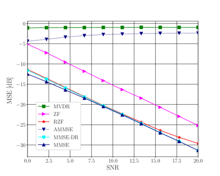
(a) $N=16$, $J=7$, SIR $=$ 0 dB

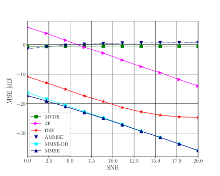
(b) $N=64$, $J=19$, , SIR $=$ 0 dB

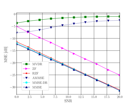
(c) $N=16$, $J=7$, SIR $=$ 10 dB

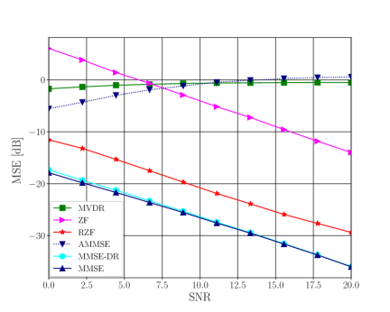
(d) $N=64$, $J=19$, SIR $=$ 10 dB

Figure 6: Performances across SNR for $\rho_{j}:=0.6$, $\beta:=0.8$, $\varepsilon_{\rho}:=0.1$, $\varepsilon_{\phi}:=\pi/12$.

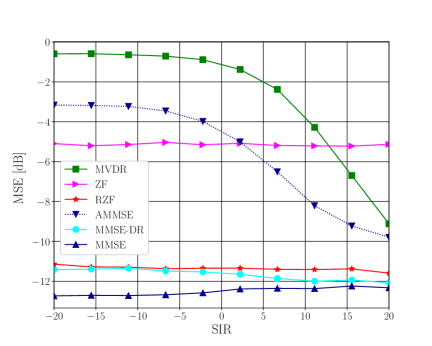
(a) $N=16$, $J=7$, SNR $=$ 0 dB

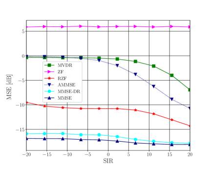
(b) $N=64$, $J=19$, SNR $=$ 0 dB

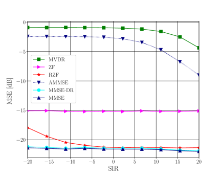
(c) $N=16$, $J=7$, SNR $=$ 10 dB

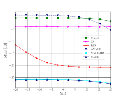
(d) $N=64$, $J=19$, SNR $=$ 10 dB

Figure 7: Performances across SIR for $\rho_{j}:=0.6$, $\beta:=0.8$, $\varepsilon_{\rho}:=0.1$, $\varepsilon_{\phi}:=\pi/12$.

A fresh look at the MSE expression in (5) may suggest that one might “exploit” the temporal correlations to reduce the MSE further, rather than bounding the leakage of interference. To see whether this active approach works, we consider an approximate MMSE (A-MMSE) beamformer under the assumption that some erroneous estimates $\hat{c}_{j}\in{\mathbb{C}}$ and $\hat{\sigma}_{0}^{2}>0$ of the correlation $c_{j}(:=E[s_{0}^{*}(k)s_{j}(k)])$ and the signal power $\sigma_{0}^{2}(:=E[\left|s_{0}(k)\right|^{2}])$ are available. To be precise, the erroneous estimates $\hat{\sigma}_{0}^{2}$ and $\hat{c}_{j}=\left|\hat{c}_{j}\right|e^{i\hat{\phi}_{j}}$ are generated, respectively, by $\hat{\sigma}_{0}^{2}:=\beta\sigma_{0}^{2}$ and $\left|\hat{c}_{j}\right|:=\left|c_{j}\right|+\varepsilon_{\rho}\sigma_{0}\sigma_{j}$, and $\hat{\phi}_{j}:=\phi_{j}+\varepsilon_{\phi}$, where $\beta\in(0,+\infty)$, $\varepsilon_{\rho}\in(-\rho_{j},1-\rho_{j})$, and $\varepsilon_{\phi}\in(-\pi,\pi]$. In this case, being free from the distortionless constraint, the MSE $J_{{\rm MSE}}({\boldsymbol{w}})$ in (3) can be approximated by $\hat{J}_{{\rm MSE}}({\boldsymbol{w}}):={\boldsymbol{w}}^{\sf H}{\boldsymbol{R}}{\boldsymbol{w}}+\hat{\sigma}_{0}^{2}(1-{\boldsymbol{w}}^{\sf H}{\boldsymbol{h}}_{0}-{\boldsymbol{h}}_{0}^{\sf H}{\boldsymbol{w}})-\sum_{j=1}^{J}(\hat{c}_{j}{\boldsymbol{w}}^{\sf H}{\boldsymbol{h}}_{j}+\hat{c}_{j}^{*}{\boldsymbol{h}}_{j}^{\sf H}{\boldsymbol{w}})$, of which the minimizer is given by ${\boldsymbol{w}}_{\rm A\mathchar 45\relax MMSE}:={\boldsymbol{R}}^{-1}\left(\hat{\sigma}_{0}^{2}{\boldsymbol{h}}_{0}+\sum_{j=1}^{J}\hat{c}_{j}{\boldsymbol{h}}_{j}\right)$. The matrix ${\boldsymbol{R}}$ is computed from 8,000 samples for all the beamformers.

Figure 3 depicts the performance of the beamformers under different temporal-correlations for SNR 0 dB and SIR 0 dB. It is seen that RZF exhibits remarkably better performances than MVDR in the strong correlation cases (cf. Remark 3.5). See Section 5.3 for discussions about the gap between the MSEs of RZF and MMSE-DR. Figure 4 shows how the performance of RZF changes according to the choice of $\varepsilon$ for SNR 0 dB and SIR 0 dB. It is seen that a wide range of the $\varepsilon$ parameter yields lower MSEs than the conventional MVDR and ZF beamformers. Figure 5 shows how the performance of A-MMSE changes due to the estimation errors in $\hat{c}_{j}$ and $\hat{\sigma}_{0}^{2}$ for $N=16$, SNR 0 dB, and SIR 0 dB. In Figure 5(a), $\varepsilon_{\phi}:=0$ and $\beta:=1$. In Figure 5(b), $\varepsilon_{\rho}:=\varepsilon_{\phi}:=0$. In contrast to the case of RZF, the performance of A-MMSE degrades by slight errors in the estimates. Figures 6 and 7 depict the performances for $\rho_{j}:=0.6$ under different SNR conditions with SIR 0 dB and 10 dB, and under different SIR conditions with SNR 0 dB and 10 dB, respectively. The results show that RZF yields near optimal performances in the case of $N:=16$ (excluding the low-SIR case in Figure 7(c)), and that it outperforms MVDR and ZF significantly over the whole settings in the case of $N:=64$. Note here that the performance of RZF for $N:=64$ is suboptimal because the large $J$ makes the minimal angular separation between the desired interfering sources be rather small. Comparing the performances of RZF for SIR $=$ 0 dB and 10 dB in Figure 6, the tendency is nearly the same; precisely, for high SNR, closer performance to MMSE is achieved in the case of SIR $=$ 10 dB than the case of SIR $=$ 0 dB. Turning our attention to Figure 7, we observe that (i) the maximum gain to MVDR is 10 dB approximately for SNR $=$ 0 dB while it is 20 dB approximately for SNR $=$ 10 dB, and (ii) MSE of RZF increases towards that of ZF as SIR decreases, more clearly for SNR $=$ 10 dB. The first observation is due to the fact that RZF as well as ZF benefits significantly from the reduction of noise. The second one is also reasonable since the zero-forcing strategy (i.e., $\epsilon:=0$) will be optimal as the interference power approaches infinity.

5.2 EEG Application

Using the interpretation of the model in (1) as the forward model used to solve the EEG inverse problem (cf. Section 2), we consider the situation when there are $J+1$ dipole sources $(J:=29)$ of brain activity and the signals are measured by an array of $N:=128$ EEG sensors. HydroCel Geodesic Sensor Net model is used as a realistic EEG cap layout. The source signals and forward model were generated using SupFunSim library [32], which utilizes FieldTrip toolbox [33] for generation of volume conduction model and leadfields. The activity $s_{0}(k)$ of the desired source is generated by an autoregressive (AR) model of order $6$, where the coefficients for each order are set to $0.2$. The interfering activities are generated by (66) with $\phi_{j}:=0$. The source activities are supposed to change in time, while their positions and orientations are assumed known and remain the same during the measurement period. The following two cases are considered: the low correlation case ($\rho_{j}:=0.5$) and the high correlation case ($\rho_{j}:=0.95$). Throughout the experiments, the power of the desired signal is fixed to $\sigma_{0}^{2}:=1$, and those of the interference and noise are changed depending on SNR and SIR, respectively. The relaxation parameter $\varepsilon$ of RZF is optimized for each SNR and SIR.

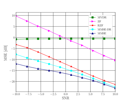
(a) $\rho_{j}:=0.5$

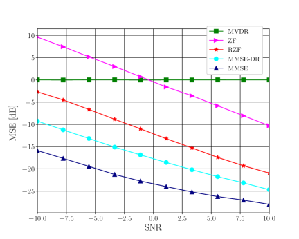
(b) $\rho_{j}:=0.95$

Figure 8: Performances for EEG application under low and high correlations (SIR $0$ dB).

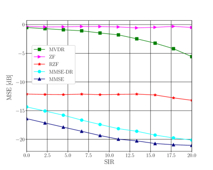
Figure 9: Performance in EEG application under low correlation $\rho_{j}:=0.5$ (SNR $0$ dB).

Figure 8 shows the results for SIR $0$ dB under different SNR conditions in the cases of (a) low correlation ($\rho_{j}:=0.5$) and (b) high correlation ($\rho_{j}:=0.95$). Figure 9 shows the results for SNR $0$ dB under different SIR conditions in the case of low correlation ($\rho_{j}:=0.5$). (The results for $\rho_{j}:=0.95$ are omitted as the results are similar.) It is seen that the RZF beamformer attains significant gains compared to the MVDR and ZF beamformers. It is also seen that its performance is fairly close to the theoretical bound (MMSE-DR) in the low correlation case with low SIR. See Section 5.3 for discussions about the MSE gap between RZF and MMSE-DR together with that for the wireless-network case.

Figure 10 shows the powers of noise and interfering activities remaining in the beamformer output for SNR $-2$ dB and SIR $0$ dB. It is seen that RZF attains an excellent tradeoff; it attains reasonably small noise-leakage by allowing some slight (invisible) leakage of the interfering activities. In Figure 10(a), the total leakage of RZF is slightly lower than the noise leakage of MVDR (see Remark 4). Figure 11(a) plots the MSE performance of RZF for each relaxation parameter $\varepsilon$ under SNR $-2$ dB, SIR $0$ dB, and $\rho_{j}:=0.5$. Within the range of $1.0<\varepsilon<1.0\times 10^{3}$, the MSE of RZF is below $-7.5$ dB. This implies that RZF is reasonably insensitive to the choice of $\varepsilon$. Figure 11(b) provides more precise information, plotting the power of noise/interference leakage contained in the beamformer output for different $\varepsilon$ values. It is seen that both noise and interference are suppressed simultaneously by RZF for an appropriately chosen $\varepsilon$. This supports the results of Figure 10(a).

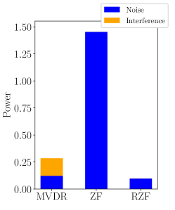
(a) $\rho_{j}:=0.5$

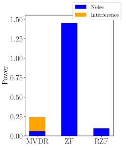
(b) $\rho_{j}:=0.95$

Figure 10: Powers of noise/interference leakage for EEG application under low and high correlations (SNR $-2$ dB, SIR $0$ dB).

\psfrag{e}[Bl][Bl][0.9]{$\varepsilon$}\includegraphics[width=225.48424pt]{fig11a.eps}

\psfrag{a}[Bl][Bl][0.9]{$\varepsilon$}\includegraphics[width=225.48424pt]{fig11b.eps}

Figure 11: Sensitivity of RZF to the parameter $\varepsilon$ for EEG application ($\rho_{j}:=0.5$, SNR $-2$ dB, SIR $0$ dB).

We now consider the adaptive implementations: RZF implemented by DDAA, and MVDR and ZF implemented by CNLMS [11]. The step sizes for all online algorithms are set to $0.1$. The parameter of the DDAA is set to $\alpha_{k}:=0.5$, $\forall k\in{\mathbb{N}}$ (see the appendix). Figure 12(a) plots the steady-state MSE of each algorithm for SIR $0$ dB and $\rho_{j}:=0.5$ under different SNR conditions. One can see that each beamformer is successfully implemented adaptively by each adaptive algorithm. Figure 12(b) plots the learning curves for the specific case of SNR $0$ dB, where each point is computed by averaging the squared errors over 300 independent trials. (For visual clarity, the MSE values are further averaged over the previous 30 iterations.) It can be seen that the MSEs of the adaptive algorithms for the RZF and ZF beamformers converge reasonably fast to those of the analytical solutions, respectively. In contrast, MVDR implemented by CNLMS converges slowly due to no use of the channel information of the interfering activities.

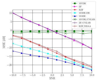
(a) steady-state performance

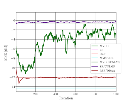
(b) learning curves under SNR $0$ dB

Figure 12: Performances of adaptive implementations for EEG application under low correlation $\rho_{j}:=0.5$ (SIR $0$ dB). RZF implemented with DDAA, and MVDR and ZF implemented both with CNLMS.

We remark finally that the RZF beamformer may be also used when surface Laplacian-processed signals are considered instead of the raw EEG signal to enhance spatial resolution [34, 35]. In such a case, the channel matrix is replaced by the surface Laplacian matrix and the covariance matrix ${\boldsymbol{R}}$ is replaced by the covariance matrix of the Laplacian-treated signal.

5.3 Discussions and Remarks

\psfrag{g}[Bc][Bl][0.9]{$\gamma$}\psfrag{i}[Bc][Bl][0.9]{Interfering source}\includegraphics[width=225.48424pt]{fig13.eps}

Figure 13: An example of the $\gamma$ value for each interfering source in the EEG application under low correlation $\rho_{j}:=0.5$ (SNR $0$ dB, SIR $0$ dB).

Figure 13 plots the $\gamma$ values for different sources in the setting corresponding to Figure 9 with SIR 0 dB. It is seen that only 9 (out of 28) sources have the $\gamma$ values within the range $(0,1)$; see (19) in Theorem 2. To see whether those interfering sources which have $\gamma$ outside the range $(0,1)$ cause the MSE gaps between RZF and MMSE-DR, we removed all such interfering sources and evaluated the MSE performances only with the remaining sources having $\gamma\in(0,1)$ under $\rho_{j}:=0.5$, SNR $-5$ dB, and SIR $0$ dB. The gap then droped, from $3.4$ dB, down to $1.5$ dB approximately. We also tested with the same number of randomly picked sources removed. In this case, the gap was no less than $2.8$ dB. This indicates that those sources having $\gamma\not\in(0,1)$ would be a main cause of the MSE gaps. In the simulation results presented in Section 5.1, there are some visible gaps between the MSEs of RZF and MMSE-DR in Figure 3(b). In the case of complex signals, Theorem 5 suggests the existence of another factor $\left(1-\left|\delta_{1}/\delta_{2}\right|^{2}\right)\sigma_{n}^{4}\tan^{2}\tau/(\sigma_{1}^{2}\cos^{2}\tau+\sigma_{n}^{2})$ that may cause the MSE gap.

Indeed, $\gamma$ is a function of $\delta_{1}$, as well as the others. Referring to (26), the sign of $\delta_{1}$ depends on the phase $\phi_{c}$ of the temporal correlation $c_{1}$. This implies that the MSE of RZF may change significantly due to the phase (or the sign in particular) of $c_{1}$. Nevertheless, the plots for RZF are nearly symmetric for the positive and negative values of $\rho_{j}(:=c_{j}/(\sigma_{0}\sigma_{j}))$. In addition, we actually tested different values of $\phi_{j}$s, which yielded no visible differences in MSE. This would be because the phase $\phi_{z_{j}}$ of the spatial correlation $z_{j}:=\left\langle{{\boldsymbol{h}}_{0}},{{\boldsymbol{h}}_{j}}\right\rangle$ is quite random among different sources.

6 Conclusion

We studied the RZF beamformer, which minimizes the output variance under the constraints of bounded interference leakage and undistorted desired signal, in the presence of temporally correlated interference. The (quadratic) relaxed zero-forcing constraint alleviates the gap between the output variance (available) and MSE (unavailable) without amplifying the noise. An adaptive implementation of the RZF beamformer based on the dual-domain adaptive algorithm was also presented. We analyzed the MSE of RZF for the single-interference case and derived the formula of MSE in terms of the spatio-temporal correlations between the desired and interfering signals as well as the variances of noise and interference, clarifying that RZF achieves the minimum MSE under the conditions. The presented analysis gave useful insights into the multiple-interference case, as discussed in the experimental section. Numerical examples showed the remarkable advantages of RZF over the MVDR and ZF beamformers. The RZF beamformer also achieved near-optimal performance in some cases. We conclude the present study by stating that the RZF beamformer will be useful particularly for the EEG brain activity reconstruction because (i) it enjoys superior performance by mitigating the interfering sources efficiently, (ii) it includes the MVDR and ZF beamformers as special cases, and (iii) it can be implemented efficiently by DDAA.

Appendix A Dual-Domain Adaptive Algorithm: An Implementation of RZF Beamformer

Given any closed convex subset $K$ of ${\mathbb{C}}^{m}$ of dimension $m$, the metric projection $P_{K}({\boldsymbol{x}})$ of a point ${\boldsymbol{x}}\in{\mathbb{C}}^{m}$ onto $K$ is defined by $P_{K}({\boldsymbol{x}}):=\operatornamewithlimits{argmin}_{{\boldsymbol{y}}\in{\mathbb{C}}^{m}}\left\|{\boldsymbol{x}}-{\boldsymbol{y}}\right\|$. The set $\{{\boldsymbol{w}}\in{\mathbb{C}}^{N}\mid\|{\boldsymbol{H}}_{\rm I}^{\sf H}{\boldsymbol{w}}\|^{2}\leq\varepsilon\}$ is a (degenerate) ellipsoid onto which the projection has no closed-form expression. Fortunately, the projection of the dual-domain vector ${\boldsymbol{H}}_{\rm I}^{\sf H}{\boldsymbol{w}}\in{\mathbb{C}}^{J}$ onto the closed ball $B_{\varepsilon}$ is easy to compute, thus used in the dual-domain algorithm. Define the normalized channel matrix $\widetilde{{\boldsymbol{H}}}_{\rm I}:={\boldsymbol{H}}_{\rm I}/\sigma_{1}({\boldsymbol{H}}_{\rm I})$. Given an initial beamforming vector ${\boldsymbol{w}}_{0}\in C$, the DDAA update equation is then given as follows:

$${\boldsymbol{w}}_{k+1}:={\boldsymbol{w}}_{k}+\lambda_{{\boldsymbol{w}},k}\eta_{k}{\boldsymbol{g}}_{k},$$

where $\lambda_{{\boldsymbol{w}},k}\in(0,2)$ and

$${\boldsymbol{g}}_{k}:= ~{}\alpha_{k}{\boldsymbol{g}}^{{\rm(1)}}_{k}+(1-\alpha_{k}){\boldsymbol{Q}}\widetilde{{\boldsymbol{H}}}_{\rm I}{\boldsymbol{g}}^{{\rm(2)}}_{k},$$

$$~{}~{}~{}~{}~{}~{}~{}~{}{\boldsymbol{Q}}:={\boldsymbol{I}}-{\boldsymbol{h}}_{0}{\boldsymbol{h}}_{0}^{\sf H}/({\boldsymbol{h}}_{0}^{\sf H}{\boldsymbol{h}}_{0}),~{}~{}~{}\alpha_{k}\in[0,1],$$

$${\boldsymbol{g}}^{{\rm(1)}}_{k}:= ~{}P_{C\cap H_{k}}({\boldsymbol{w}}_{k})-{\boldsymbol{w}}_{k}=-\frac{{\boldsymbol{w}}_{k}^{\sf H}{\boldsymbol{y}}(k)}{{\boldsymbol{y}}(k)^{\sf H}{\boldsymbol{Q}}{\boldsymbol{y}}(k)}{\boldsymbol{Q}}{\boldsymbol{y}}(k),$$

$$~{}~{}~{}~{}~{}~{}~{}~{}H_{k}:=\{{\boldsymbol{w}}\in{\mathbb{C}}^{N}\mid{{\boldsymbol{w}}}^{\sf H}{\boldsymbol{y}}(k)=0\},$$

$${\boldsymbol{g}}^{{\rm(2)}}_{k}:= ~{}P_{B_{\varepsilon}}\left(\widetilde{{\boldsymbol{H}}}_{\rm I}^{\sf H}{\boldsymbol{w}}_{k}\right)-\widetilde{{\boldsymbol{H}}}_{\rm I}^{\sf H}{\boldsymbol{w}}_{k}$$

$$= ~{}\begin{cases}\Bigg{(}\dfrac{\sqrt{\varepsilon}}{\left\|\widetilde{{\boldsymbol{H}}}_{\rm I}^{\sf H}{\boldsymbol{w}}_{k}\right\|}-1\Bigg{)}\widetilde{{\boldsymbol{H}}}_{\rm I}^{\sf H}{\boldsymbol{w}}_{k},&\mbox{if }\left\|\widetilde{{\boldsymbol{H}}}_{\rm I}^{\sf H}{\boldsymbol{w}}_{k}\right\|^{2}>\varepsilon,\\ {\boldsymbol{0}},&\mbox{if }\left\|\widetilde{{\boldsymbol{H}}}_{\rm I}^{\sf H}{\boldsymbol{w}}_{k}\right\|^{2}\leq\varepsilon,\end{cases}$$

$$\eta_{k}:= ~{}\begin{cases}\dfrac{\alpha_{k}{\big{\|}}{\boldsymbol{g}}^{{\rm(1)}}_{k}{\big{\|}}^{{\rm 2}}+(1-\alpha_{k})\left\|{\boldsymbol{g}}_{k}^{(2)}\right\|^{2}}{\left\|{\boldsymbol{g}}_{k}\right\|^{2}},&\mbox{if }{\boldsymbol{g}}_{k}\neq{\boldsymbol{0}},\\ 1,&\mbox{otherwise.}\end{cases}$$

Here, the vector ${\boldsymbol{g}}_{k}^{{\rm(1)}}$ contributes to reducing the output variance in (6a), while ${\boldsymbol{g}}_{k}^{{\rm(2)}}$ contributes to reducing the violation of the quadratic constraint of (6d). The DDAA method has been proven to generate a sequence convergent to an asymptotically optimal point under certain mild conditions. See [22, 21] for the detailed properties of the algorithm.

References

• [1] H. L. Van Trees, Optimum Array Processing: Part IV of Detection, Estimation, and Modulation Theory, New York: Wiley, 2002.
• [2] S. Sun, T. Rappaport, R.W. Heath, Jr., A. Nix, S. Rangan, MIMO for millimeter-wave wireless communications: Beamforming, spatial multiplexing, or both?, IEEE Communications Magazine 52 (12) (2014) 110–121.
• [3] P. Taiwo, A. Cole-Rhodes, Adaptive beamforming for multiple-access millimeter wave communications, in: Proc. Annual Conference on Information Sciences and Systems, 2019.
• [4] A. Bana, E. de Carvalho, B. Soret, T. Abrão, J. C. Marinello, E. G. Larsson, P. Popovski, Massive MIMO for Internet of Things (IoT) connectivity, Physical Communications 37 (2019) 1–17.
• [5] B. D. Van Veen, W. Van Drongelen, M. Yuchtman, A. Suzuki, Localization of brain electrical activity via linearly constrained minimum variance spatial filtering, IEEE Transactions on biomedical engineering 44 (9) (1997) 867–880.
• [6] H. B. Hui, D. Pantazis, S. L. Bressler, R. M. Leahy, Identifying true cortical interactions in MEG using the nulling beamformer, NeuroImage 49 (4) (2010) 3161–3174.
• [7] S. S. Dalal, K. Sekihara, S. S.Nagarajan, Modified beamformers for coherent source region suppression, IEEE Transactions on Biomedical Engineering 53 (7) (2006) 1357–1363.
• [8] H. B. Hui, R. M. Leahy, Linearly constrained MEG beamformers for MVAR modeling of cortical interactions, in: IEEE International Symposium on Biomedical Imaging: Nano to Macro, IEEE, 2006, pp. 237–240.
• [9] T. Piotrowski, J. Nikadon, D. Gutiérrez, MV-PURE spatial filters with application to EEG/MEG source reconstruction, IEEE Transactions on Signal Processing 67 (3) (2019) 553–567.
• [10] O. L. Frost, An algorithm for linearly constrained adaptive array processing, Proceedings of the IEEE 60 (1972) 926–935.
• [11] J. A. Apolinário, S. Werner, P. S. Diniz, T. I. Laakso, Constrained normalized adaptive filters for CDMA mobile communications, in: Signal Processing Conference (EUSIPCO 1998), 9th European, IEEE, 1998, pp. 1–4.
• [12] N. Owsley, Noise cancellation in the presence of correlated signal and noise, Tech. Rep. 4639, Naval Underwater Systems Center (Jan. 1974).
• [13] B. Wittevrongel, M. M. V. Hulle, Hierarchical online SSVEP spelling achieved with spatiotemporal beamforming, in: IEEE Statistical Signal Processing Workshop (SSP), 2016.
• [14] M. Mahmoodi, B. M. Abadi, H. Khajepur, M. H. Harirchian, A robust beamforming approach for early detection of readiness potential with application to brain-computer interface systems, in: Annual International Conference of the IEEE Engineering in Medicine and Biology Society (EMBC), 2017, pp. 2980–2983.
• [15] S. Boe, A. Gionfriddo, S. Kraeutner, A. Tremblay, G. Little, T. Bardouille, Laterality of brain activity during motor imagery is modulated by the provision of source level neurofeedback, NeuroImage 101 (2014) 159 – 167.
• [16] S. Enriquez-Geppert, R. J. Huster, C. S. Herrmann, EEG-neurofeedback as a tool to modulate cognition and behavior: A review tutorial, Frontiers in Human Neuroscience 11 (2017) 19 pages.
• [17] T. R. Mullen, C. A. E. Kothe, Y. M. Chi, A. Ojeda, T. Kerth, S. Makeig, T. Jung, G. Cauwenberghs, Real-time neuroimaging and cognitive monitoring using wearable dry EEG, IEEE Transactions on Biomedical Engineering 62 (11) (2015) 2553–2567.
• [18] T. Hartmann, I. Lorenz, N. Müller, B. Langguth, N. Weisz, The effects of neurofeedback on oscillatory processes related to tinnitus, Brain Topography 27 (1) (2014) 149–157.
• [19] R. van Lutterveld, S. D. Houlihan, P. Pal, M. D. Sacchet, C. McFarlane-Blake, P. R. Patel, J. S. Sullivan, A. Ossadtchi, S. Druker, C. Bauer, J. A. Brewer, Source-space EEG neurofeedback links subjective experience with brain activity during effortless awareness meditation, NeuroImage 151 (2017) 117 – 127.
• [20] M. Yukawa, Y. Sung, G. Lee, Adaptive interference suppression in mimo multiple access channels based on dual-domain approach, in: Proc. ITC-CSCC, 2011.
• [21] M. Yukawa, Y. Sung, G. Lee, Dual-domain adaptive beamformer under linearly and quadratically constrained minimum variance, IEEE Transactions on Signal Processing 61 (11) (2013) 2874–2886.
• [22] M. Yukawa, K. Slavakis, I. Yamada, Multi-domain adaptive learning based on feasibility splitting and adaptive projected subgradient method, IEICE Trans. Fundamentals E93-A (2) (2010) 456–466.
• [23] T. Kono, M. Yukawa, T. Piotrowski, Beamformer design under time-correlated interference and online implementation: Brain-activity reconstruction from EEG, in: Proc. IEEE ICASSP, 2019, pp. 1070–1074.
• [24] R. Hoctor, S. Kassam, The unifying role of the coarray in aperture synthesis for coherent and incoherent imaging, Proceedings of the IEEE 78 (4) (1990) 735–752.
• [25] P. Pal, P. P. Vaidyanathan, Nested arrays: A novel approach to array processing with enhanced degrees of freedom, IEEE Transactions on Signal Processing 58 (8) (2010) 4167–4181.
• [26] C.-L. Liu, P. P. Vaidyanathan, Super nested arrays: Linear sparse arrays with reduced mutual coupling — Part I: Fundamentals, IEEE Transactions on Signal Processing 64 (15) (2016) 3997–4012.
• [27] C. Zhou, Y. Gu, X. Fan, Z. Shi, G. Mao, Y. D. Zhang, Direction-of-arrival estimation for coprime array via virtual array interpolation, IEEE Transactions on Signal Processing 66 (22) (2018) 5956–5971.
• [28] Z. Zheng, W.-Q. Wang, Y. Kong, Y. D. Zhang, MISC array: A new sparse array design achieving increased degrees of freedom and reduced mutual coupling effect, IEEE Transactions on Signal Processing 67 (7) (2019) 1728–1741.
• [29] Z. Li, Z. Xiaofei, G. Pan, W. Cheng, Sparse nested linear array for direction of arrival estimation, Signal Processing 169 (2020) 1–9.
• [30] T. Kailath, A. H. Sayed, B. Hassibi, Linear Estimation, Prentice Hall, Upper Saddle River, New Jersey, 2000.
• [31] R. A. Horn, C. R. Johnson, Matrix Analysis, Cambridge University Press, New York, 1985.
• [32] K. Rykaczewski, J. Nikadon, W. Duch, T. Piotrowski, SUPFUNSIM: Spatial filtering toolbox for EEG, Neuroinform 19 (2021) 107–125.
• [33] R. Oostenveld, P. Fries, E. Maris, J.-M. Schoffelen, FieldTrip: Open source software for advanced analysis of MEG, EEG, and invasive electrophysiological data, Computational Intelligence and Neuroscience (2011) 9 pages.
• [34] V. Murzin, A. Fuchs, J. Kelso, Detection of correlated sources in EEG using combination of beamforming and surface Laplacian methods, Journal of Neuroscience Methods 218 (1) (2013) 96–102.
• [35] J. Kayser, C. Tenke, Issues and considerations for using the scalp surface Laplacian in EEG/ER research: A tutorial review, International Journal of Psychophysiology 97 (3) (2015) 189–209.