Dzyaloshinskii interaction and exchange-relativistic effects in orthoferrites

Аннотация

We present an overview of the microscopic theory of the Dzyaloshinskii-Moriya (DM) coupling and related exchange-relativistic effects such as exchange anisotropy, electron-nuclear antisymmetric supertransferred hyperfine interactions, antisymmetric magnetogyrotropic effects, and antisymmetric magnetoelectric coupling in strongly correlated 3$d$ compounds focusing on orthoferrites RFeO₃ (R is a rare-earth ion or yttrium Y). Most attention in the paper centers around the derivation of the Dzyaloshinskii vector, its value, orientation, and sense (sign) under different types of the (super)exchange interaction and crystal field. Microscopically derived expression for the dependence of the Dzyaloshinskii vector on the superexchange geometry allows one to find all the overt and hidden canting angles in orthoferrites RFeO₃ as well as corresponding contribution to magnetic anisotropy. Being based on the theoretical predictions regarding the sign of the Dzyaloshinskii vector we have predicted and study in detail a novel magnetic phenomenon, weak ferrimagnetism in mixed weak ferromagnets with competing signs of the Dzyaloshinskii vectors. The ligand NMR measurements in weak ferromagnets are shown to be an effective tool to inspect the effects of DM coupling in an external magnetic field. Along with orthoferrites RFeO₃ and weak ferrimagnets RFe_1-xCr_xO₃, although to a lesser extent, we address such typical weak ferromagnets as $\alpha$-Fe₂O₃, FeBO₃, and FeF₃.

1 Introduction

It is not often in the history of science that one paper of an author opens up a novel field of theoretical and experimental research. This is exactly what happened with the article by Igor Dzyaloshinskii [1], devoted to the explanation of the phenomenon of weak ferromagnetism.

More than a hundred years have passed after T. Smith [2] found in 1916 a weak, or $parasitic$ ferromagnetism in an "international family line"of different natural hematite $\alpha$-Fe₂O₃ single crystalline samples from Italy, Hungary, Brasil, and Russia (Schabry, Ural Mountains, near Ekaterinburg) that was assigned to ferromagnetic impurities. Later the phenomenon was observed in many other materials, in fluoride NiF₂ with rutile structure, in the orthorhombic orthoferrites RFeO₃ (where R is a rare-earth element or Y), in rhombohedral antiferromagnets MnCO₃, NiCO₃, CoCO₃, and FeBO₃. However, only in 1954 L. M. Matarrese and J. W. Stout for NiF₂ [3] and in 1956 A. S. Borovik-Romanov and M. P. Orlova for very pure synthesised carbonates MnCO₃ and CoCO₃ [4] have firmly established that weak ferromagnetism is observed in chemically pure antiferromagnetic materials and therefore it is an intrinsic property of some antiferromagnets, the connexion between the weak ferromagnetism and any impurities or inhomogeneities seems very unlikely. Furthermore, Borovik-Romanov and Orlova assigned the uncompensated moment in MnCO₃ and CoCO₃ to an overt canting of the two magnetic sublattices in almost antiferromagnetic matrix. The model of a canted antiferromagnet became generally adopted model of the weak ferromagnet.

A theoretical explanation and first thermodynamic theory for weak ferromagnetism in $\alpha$-Fe₂O₃, MnCO₃, and CoCO₃ was provided by I. E. Dzyaloshinskii (Dzialoshinskii, Dzyaloshinsky) [1] in 1957 on the basis of symmetry considerations and Landau’s theory of phase transitions of the second kind.

Free energy of the two-sublattice uniaxial weak ferromagnet such as $\alpha$-Fe₂O₃, MnCO₃, CoCO₃, FeBO₃ was shown to be written as follows

$$F=MH_{E}({\bf m}_{1}\cdot{\bf m}_{2})-M{\bf H}_{0}({\bf m}_{1}+{\bf m}_{2})+E_{D}+E_{A}$$

$$=MH_{E}({\bf m}^{2}-{\bf l}^{2})-M{\bf H}_{0}{\bf m}+E_{D}+E_{A}\,.$$ (1)

In this expression ${\bf m}_{1}$ and ${\bf m}_{2}$ are unit vectors in the directions of the sublattice moments, $M$ is the sublattice magnetization, ${\bf m}=\frac{1}{2}({\bf m}_{1}+{\bf m}_{2})$ and ${\bf l}=\frac{1}{2}({\bf m}_{1}-{\bf m}_{2})$ are the ferro- and antiferromagnetic vectors, respectively, $H_{0}$ is the applied field, $H_{E}$ is the exchange field,

$$E_{D}=-MH_{D}[{\bf m}_{1}\times{\bf m}_{2}]_{z}=+2MH_{D}[{\bf m}\times{\bf l}]_{z}=\\$$

$$+2MH_{D}(m_{x}l_{y}-m_{y}l_{x})$$ (2)

is now called the Dzyaloshinskii interaction, $H_{D}$ $>$ 0 is the Dzyaloshinskii field. The anisotropy energy $E_{A}$ is assumed to have the form: $E_{A}=H_{A}/2M(m_{1z}^{2}+m_{2z}^{2})=2H_{A}/2M(m_{z}^{2}+l_{z}^{2})$, where $H_{A}$ is the anisotropy field. The choice of sign for the anisotropy field $H_{A}$ assumes that the $c$ axis is a hard direction of magnetization. In a general sense the Dzyaloshinskii interaction implies the terms that are linear both on ferro- and antiferromagnetic vectors. For instance, in orthorhombic orthoferrites and orthochromites the Dzyaloshinskii interaction consists of the antisymmetric and symmetric terms

$$E_{D}=d_{1}m_{z}l_{x}+d_{2}m_{x}l_{z}=$$

$$\frac{d_{1}-d_{2}}{2}(m_{z}l_{x}-m_{x}l_{z})+\frac{d_{1}+d_{2}}{2}(m_{z}l_{x}+m_{x}l_{z})=$$

$$-2MH_{D}[{\bf m}\times{\bf l}]_{y}+\frac{d_{1}+d_{2}}{2}(m_{z}l_{x}+m_{x}l_{z})\,,$$ (3)

while for tetragonal fluorides NiF₂ and CoF₂ the Dzyaloshinskii interaction consists of the only symmetric term. Despite Dzyaloshinskii supposed that weak ferromagnetism is due to relativistic spin-lattice and magnetic dipole interaction, the theory was phenomenological one and did not clarify the microscopic nature of the Dzyaloshinskii interaction that does result in the canting. Later on, in 1960, T. Moriya [5] suggested a model microscopic theory of the exchange-relativistic antisymmetric exchange interaction to be a main contributing mechanism of weak ferromagnetism

$$V_{DM}=\sum_{mn}({\bf d}_{mn}\cdot\left[{\bf S}_{m}\times{\bf S}_{n}\right])\,,$$ (4)

now called Dzyaloshinskii-Moriya (DM) spin coupling. Here, ${\bf d}_{mn}$ is the axial Dzyaloshinskii vector. Presently Keffer [6] proposed a simple phenomenological expression for the Dzyaloshinskii vector for two magnetic ions M_i and M_j interacting by the superexchange mechanism via intermediate ligand O (see Fig. 1):

$$\mathbf{d}_{ij}\propto[\mathbf{r}_{i}\times\mathbf{r}_{j}]\,,$$ (5)

where ${\bf r}_{i,j}$ are unit radius vectors for O - M_i,j bonds with presumably equal bond lenghts. Later on Moskvin [7] derived a microscopic formula for Dzyaloshinskii vector

$$\mathbf{d}_{ij}=d_{ij}(\theta)[\mathbf{r}_{i}\times\mathbf{r}_{j}]\,,$$ (6)

where

$$d_{ij}(\theta)=d_{1}(R_{i},R_{j})+d_{2}(R_{i},R_{j})cos\theta_{ij}$$ (7)

with $\theta_{ij}$ being the M_i - O - M_j bonding angle. The sign of the scalar parameter $d_{ij}(\theta)$ can be addressed to be the sign (sense) of the Dzyaloshinskii vector. The formula (6) was shown to work only for $S$-type magnetic ions with orbitally nondegenerate ground state, e.g. for 3$d$-ions with half-filled shells (3$d^{5}$ or $t_{2g}^{3}$, $t_{2g}^{3}e_{g}^{2}$, $t_{2g}^{6}e_{g}^{2}$).

It should be noted that sometimes instead of (6) one may use another form of the structural factor for the Dzyaloshinskii vector:

$$\left[{\bf r}_{1}\times{\bf r}_{2}\right]=\frac{1}{2}\left[({\bf r}_{1}-{\bf r}_{2})\times({\bf r}_{1}+{\bf r}_{2})\right]=\frac{1}{2l^{2}}\left[{\bf R}_{12}\times{\boldsymbol{\rho}}_{12}\right]\,,$$ (8)

where ${\bf R}_{12}={\bf R}_{1}-{\bf R}_{2}$, ${\boldsymbol{\rho}}_{12}=({\bf R}_{1}+{\bf R}_{2})$.

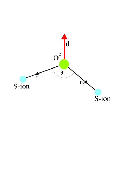
Рис. 1: (Color online) Superexchange geometry and the Dzyaloshinskii vector.

Таблица 1: Main exchange and DM coupling parameters in orthoferrites compared with other weak ferromagnets (WFMs), $I$ is the exchange integral, $\alpha_{D}$ is the canting angle. See text for detail.

WFM	RFeO, Å	$\theta$	TN, K	$I$, K (MFA)	HE, Tesla	$\alpha_{D}$	HD, Tesla	$d$($\theta$), K
YFeO3	2.001 (x2)	145∘	640	36.6	640	$1.1\cdot 10^{-2}$	14	3.2
$\alpha$-Fe2O3	2.111	145∘	948	54.2	870-920	$1.1\cdot 10^{-3}$	1.9-2.2	2.3
FeBO3	2.028	126∘	348	19.9	300	$1.7\cdot 10^{-2}$	10	2.3
FeF3	1.914	153∘	363	20.7	440	$5.5\cdot 10^{-3}$	4.88	1.1

Starting with the pioneering papers by Dzyaloshinskii [1] and Moriya [5] the DM coupling was extensively investigated in 60-80ths in connection with the weak ferromagnetism focusing on hematite $\alpha$-Fe₂O₃ and orthoferrites RFeO₃ [8, 9, 10, 11] (see, also review articles Refs. [12, 13]). Typical values of the canting angle $\alpha_{D}$ turned out to be on the order of 0.001-0.01, in particular, $\alpha_{D}=1.1\cdot 10^{-3}$ in $\alpha$-Fe₂O₃ [14], 2.2-2.9$\cdot 10^{-3}$ in La₂CuO₄ [15], $5.5\cdot 10^{-3}$ in FeF₃ [16], $1.1\cdot 10^{-2}$ in YFeO₃ [17], $1.7\cdot 10^{-2}$ in FeBO₃ [18] (see Table 1).

V. I. Ozhogin et al. [19] in 1968 first raised the issue of the sign of the Dzyaloshinskii vector, however, only in 1990 the reliable local information on the sign of the Dzyaloshinskii vector, or to be exact, that of the Dzyaloshinskii parameter $d_{12}$, was first extracted from the ¹⁹F ligand NMR (nuclear magnetic resonance) data in weak ferromagnet FeF₃ [20]. In 1977 we have shown that the Dzyaloshinskii vectors can be of opposite sign for different pairs of $S$-type ions [10] that allowed us to uncover a novel magnetic phenomenon, weak ferrimagnetism, and a novel class of magnetic materials, weak ferrimagnets, which are systems such as solid solutions YFe_1-xCr_xO₃ with competing signs of the Dzyaloshinskii vectors and the very unusual concentration and temperature dependence of the magnetization[21]. The relation between Dzyaloshinskii vector and the superexchange geometry (6) allowed us to find numerically all the overt and hidden canting angles in the rare-earth orthoferrites [9] that was nicely confirmed in ⁵⁷Fe NMR [22] and neutron diffraction [23] measurements.

The stimulus to a renewed interest to the subject was given by the cuprate problem, in particular, by the weak ferromagnetism observed in the parent cuprate La₂CuO₄ [15] and many other interesting effects for the DM systems, in particular, the "field-induced gap"  phenomena [24]. At variance with typical 3D systems such as orthoferrites, the cuprates are characterised by a low-dimensionality, large diversity of Cu-O-Cu bonds including corner- and edge-sharing, different ladder configurations, strong quantum effects for $s=1/2$ Cu²⁺ centers, and a particularly strong Cu-O covalency resulting in a comparable magnitude of hole charge/spin densities on copper and oxygen sites. Several groups (see, e.g., Refs.[25, 26, 27]) developed the microscopic model approach by Moriya for different 1D and 2D cuprates, making use of different perturbation schemes, different types of low-symmetry crystalline field, different approaches to intra-atomic electron-electron repulsion. However, despite a rather large number of publications and hot debates (see, e.g., Ref.[28]) the problem of exchange-relativistic effects, that is of antisymmetric exchange and related problem of spin anisotropy in cuprates remains to be open (see, e.g., Refs.[13, 29, 30, 31] for recent experimental data and discussion). Common shortcomings of current approaches to DM coupling in 3$d$ oxides concern a problem of allocation of the Dzyaloshinskii vector and respective "weak"(anti)ferromagnetic moments, and full neglect of spin-orbital effects for "nonmagnetic"oxygen O^2- ions, which are usually believed to play only indirect intervening role. From the other hand, the oxygen ¹⁷O NMR-NQR studies of weak ferromagnet La₂CuO₄[32, 33] seem to evidence unconventional local oxygen "weak-ferromagnetic"polarization whose origin cannot be explained in frames of current models.

All the systems described above were somehow or other connected with insulating weak ferromagnets where DM coupling manifests itself in the canting of a basic antiferromagnetic structure. However, DM coupling can induce helimagnetic distortion of the ferromagnetic order as in caesium cupric chloride, CsCuCl₃ to be a unique screw antiferroelectric crystal (see, e.g., Ref. [13] and references therein). In fact, it is known for a long time that the DM coupling can produce long-period magnetic spiral structures in ferromagnetic and antiferromagnetic crystals lacking inversion symmetry. This effect was suggested for metallic MnSi and other crystals with B20 structure, and it has been carefully proved that the sign of the DM coupling, hence the sign of the spin helix, is determined by the crystal handedness.

Phenomenologically antisymmetric DM coupling in a continual approximation gives rise to so-called Lifshitz invariants, energy contributions linear in first spatial derivatives of the magnetization ${\bf m}({\bf r})$ [34]

$$m_{i}\frac{\partial m_{j}}{\partial x_{l}}-m_{j}\frac{\partial m_{i}}{\partial x_{l}}$$ (9)

($x_{l}$ is a spatial coordinate). These chiral interactions derived from the DM coupling stabilize localized (vortices) and spatially modulated structures with a fixed rotation sense of the magnetization [35]. In fact, these are the only mechanism to induce nanosize skyrmion structures in condensed matter. Despite a clear weakness of the typical DM coupling as compared with typical isotropic exchange interactions the DM coupling can be a central ingredient in the stabilization of complex magnetic textures.

The DM coupling contribution to a micromagnetic free energy density $F({\bf r})$ is usually represented as follows

$$F({\bf r})=\sum_{i}{\bf D}_{i}({\bf m}({\bf r}))\cdot\left[{\bf m}({\bf r})\times\frac{\partial{\bf m}({\bf r})}{\partial r_{i}}\right]\,,$$ (10)

where the Dzyaloshinskii vectors ${\bf D}_{i}({\bf m}({\bf r}))$ are considered generally to depend on magnetization direction ${\bf m}({\bf r})$ [36]. Within ab initio density functional theory (DFT) methods, DM coupling is often computed by adding spin-orbital interaction perturbatively to spirals with finite wavevectors ${\bf q}$ and extracting $D_{j}$ from the $q$-linear term in the dispersion $E({\bf q})$. However, nearly exclusively, theoretical studies in this context were in the past bound to pure spin models without itinerancy, leaving the impact of charge fluctuations aside.

In recent years interest has shifted towards other manifestation of the DM coupling, such as the magnetoelectric effect [37, 38, 39], where reliable theoretical predictions have been lacking. All this stimulated the critical revisit of many old approaches to the spin-orbital effects in 3$d$ oxides, starting from the choice of proper perturbation scheme and effective spin Hamiltonian model, implied usually only indirect intervening role played by "nonmagnetic"  oxygen O^2- ions.

In this paper we present an overview of the microscopic theory of the DM coupling and other related exchange-relativistic effects focusing on orthoferrites RFeO₃. The rest part of the paper is organized as follows. In Sec. 2 we shortly address main results of the microscopic theory of the isotropic superexchange interactions for so-called $S$-type ions focusing on the angular dependence of the exchange integrals. Sec. 3 is devoted to microscopic theory of the DM coupling. Starting with Moriya’s theory we arrive at a more comprehensive derivation of the Dzyaloshinskii vector for the $S$-type 3$d$-ions, its value, orientation, and sense (sign) under different types of the (super)exchange interaction and crystal field. Here we consider the DM coupling with participation of rare-earth ions. Theoretical predictions of this section are compared in Sec. 4 with experimental data for the overt and hidden canting, as well as magnetic anisotropy in orthoferrites. In Sec. 5 we address unconventional properties of weak ferrimagnetism as a novel type of magnetic ordering in systems with competing signs of the Dzyaloshinskii vector, in particular, features of the 4$f$ - 3$d$ interaction in weak ferrimagnets RFe_1-xCr_xO₃, and unconventional spin-reorientation transitions in weak ferrimagnets. In Sec. 6 we discuss several experimental tools to examine the sign of the Dzyaloshinskii vector, including $\mu$SR of positive muons and ligand NMR in weak ferromagnets. Last part of the article is devoted to related exchange-relativistic effects, in particular, to exchange-relativistic two-ion anisotropy (Sec. 7), antisymmetric supertransferred hyperfine interaction as electron-nuclear counterpart of DM coupling (Sec. 8), antisymmetric exchange-relativistic spin-other-orbit coupling determining unconventional magnetooptics of weak ferromagnets (Sec. 9), and antisymmetric exchange-relativistic spin-dependent electric polarization (Sec. 10). A brief conclusion is made in Sec. 11.

2 Microscopic theory of the isotropic superexchange coupling

DM coupling is derived from the off-diagonal (super)exchange coupling and does usually accompany a conventional (diagonal) Heisenberg type isotropic (super)exchange coupling:

$${\hat{V}}_{ex}=J_{12}({\bf S}_{1}\cdot{\bf S}_{2})\,.$$ (11)

The modern microscopic theory of the (super)exchange coupling had been elaborated by many physicists starting with well-known papers by P. Anderson [40], especially intensively in 1960-70th (see review articles [41]). Numerous papers devoted to the problem pointed to existence of many hardly estimated exchange mechanisms, seemingly comparable in value, in particular, for superexchange via intermediate ligand ion to be the most interesting for strongly correlated systems such as 3$d$ oxides. Unfortunately, up to now we have no reliable estimations of the exchange parameters, though from the other hand we have no reliable experimental information about their magnitudes. To that end, many efforts were focused on the fundamental points such as many-electron theory and orbital dependence [42, 43, 7, 44], crystal-field effects [45], off-diagonal exchange [46], exchange in excited states [47], angular dependence of the superexchange coupling [7]. The irreducible tensor operators (the Racah algebra) were shown to be very instructive tool both for description and analysis of the exchange coupling in the 3$d$- and 4$f$-systems [42, 43, 7, 44, 45].

First poor man’s microscopic derivation for the dependence of the superexchange integral on the bonding angle (see Fig. 1) was performed by the author in 1970 [7] under simplified assumptions. For the $S$-ions with configuration 3$d^{5}$ (Fe³⁺, Mn²⁺) the angular dependence of the superexchange integral is

$$J_{12}(\theta)=a+b\cdot cos\theta_{12}+c\cdot cos^{2}\theta_{12}\,,$$ (12)

where parameters $a$, $b$, $c$ depend on the cation-ligand separation. Parameters $a$ and $c$ are related with the contribution of the intermediate ligand 2$p$ shell, while the $\propto\cos\theta_{12}$ term is related with the low-energy ligand inter-configurational $2p\rightarrow 3s$ excitations.

Later on the derivation had been generalized for the 3$d$ ions in a strong cubic crystal field [11]. Orbitally isotropic contribution to the exchange integral for pair of 3$d$-ions with configurations $t_{2g}^{n_{1}}e_{g}^{n_{2}}$ can be written as follows

$$J=\sum_{\gamma_{i},\gamma_{j}}J(\gamma_{i}\gamma_{j})\,(g_{\gamma_{i}}-1)\,(g_{\gamma_{j}}-1)\,,$$ (13)

where $g_{\gamma_{i}},g_{\gamma_{j}}$ are effective "$g$-factors"of the $\gamma_{i},\gamma_{j}$ subshells of ion 1 and 2, respectively:

$$g_{\gamma_{i}}=1+\frac{S(S+1)+S_{i}(S_{i}+1)-S_{j}(S_{j}+1)}{2S(S+1)}\,.$$ (14)

Kinetic exchange contribution to partial exchange parameters $I(\gamma_{i}\gamma_{j})$ related with the electron transfer to partially filled shells can be written as follows [45, 11]

$$J(e_{g}e_{g})=\frac{(t_{ss}+t_{\sigma\sigma}cos\theta)^{2}}{2U};\,J(e_{g}t_{2g})=\frac{t_{\sigma\pi}^{2}}{3U}sin^{2}\theta;$$

$$J(t_{2g}t_{2g})=\frac{2t_{\pi\pi}^{2}}{9U}(2-sin^{2}\theta)\,,$$ (15)

where $t_{\sigma\sigma}>t_{\pi\sigma}>t_{\pi\pi}>t_{ss}$ are positive definite $d$–$d$ transfer integrals, $U$ is a mean $d$–$d$ transfer energy (correlation energy). All the partial exchange integrals appear to be positive or "antiferromagnetic irrespective of the bonding angle value, though the combined effect of the $ss$ and $\sigma\sigma$ bonds $\propto cos\theta$ in $J(e_{g}e_{g})$ yields a ferromagnetic contribution given bonding angles $\pi/2<\theta<\pi$. It should be noted that the "large"ferromagnetic potential contribution [48] has a similar angular dependence [47].

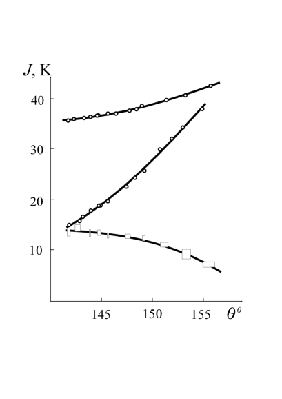
Рис. 2: Dependence of the Fe³⁺ - Fe³⁺, Cr³⁺ - Cr³⁺, Fe³⁺ - Cr³⁺ exchange integrals on the superexchange bond angle in orthoferrites-orthocromites [49].

Some predictions regarding the relative magnitude of the $J(\gamma_{i}\gamma_{j})$ exchange parameters can be made using the relation among different $d$–$d$ transfer integrals as follows

$$t_{\sigma\sigma}\,:\,t_{\pi\sigma}\,:\,t_{\pi\pi}\,:\,t_{ss}\approx\lambda_{\sigma}^{2}\,:\,\lambda_{\pi}\lambda_{\sigma}\,:\,\lambda_{\pi}^{2}\,:\,\lambda_{s}^{2}\,,$$ (16)

where $\lambda_{\sigma},\lambda_{\pi},\lambda_{s}$ are covalency parameters. The simplified kinetic exchange contribution (15) related with the electron transfer to partially filled shells does not account for intra-center correlations which are of a particular importance for the contribution related with the electron transfer to empty shells. For instance, appropriate contributions related with the transfer to empty $e_{g}$ subshell for the Cr³⁺ - Cr³⁺ and Fe³⁺ - Cr³⁺ exchange integrals are

$$\Delta J_{CrCr}=-\frac{\Delta E(35)}{6U}\frac{t_{\sigma\pi}^{2}}{U}sin^{2}\theta\,;$$

$$\Delta J_{FeCr}=-\frac{\Delta E(35)}{10U}\left[\frac{(t_{ss}+t_{\sigma\sigma}cos\theta)^{2}}{U}+\frac{t_{\sigma\pi}^{2}}{U}sin^{2}\theta\right]\,,$$ (17)

where $\Delta E(35)$ is the energy separation between ${}^{3}E_{g}$ and ${}^{5}E_{g}$ terms for $t_{2g}^{3}e_{g}$ configuration (Cr²⁺ ion). Obviously these contributions have a ferromagnetic sign. Furthermore, the exchange integral $J(CrCr)$ can change sign at $\theta$ = $\theta_{cr}$:

$$sin^{2}\theta_{cr}=\frac{1}{\left(\frac{1}{2}+\frac{3}{8}\frac{\Delta E(35)}{U}\frac{t^{2}_{\sigma\pi}}{t^{2}_{\pi\pi}}\right)}\,.$$ (18)

Microscopically derived angular dependence of the superexchange integrals does nicely describe the experimental data for exchange integrals $J(FeFe)$, $J(CrCr)$, and $J(FeCr)$ in orthoferrites, orthochromites, and orthoferrites-orthochromites [49] (see Fig. 2). The fitting allows us to predict the sign change for $J(CrCr)$ and $J(FeCr)$ at $\theta_{12}$ $\approx$ 133^∘ and 170^∘, respectively. In other words, the Cr³⁺ - O^2- - Cr³⁺ (Fe³⁺ - O^2- - Cr³⁺) superexchange coupling becomes ferromagnetic at $\theta_{12}\leq 133^{\circ}$ ($\theta_{12}\geq 170^{\circ}$). However, it should be noted that too narrow (141^∘– 156^∘) range of the superexchange bonding angles we used for the fitting with assumption of the same Fe(Cr)-O bond separations and mean superexchange bonding angles for all the systems gives rise to a sizeable parameter’s uncertainty, in particular, for $J(FeFe)$ and $J(FeCr)$. In addition it is necessary to note a large uncertainty regarding what is here called the "experimental"  value of the exchange integral. The fact is that the "experimental"  exchange integrals we have just used above are calculated using simple MFA (mean-field approximation) relation

$$T_{N}=\frac{zS(S+1)}{3k_{B}}J\,,$$ (19)

however, this relation yields the exchange integrals ($J$ = 36.8 K in YFeO₃) that can be one and a half or even twice less than the values obtained by other methods [11, 50, 51]. Most recent precise experimental data yield for YFeO₃ $J_{c}$ = 58.2 K, $J_{ab}$ = 53.6 K [52] or $J_{c}$ = $J_{ab}$ = 51.5 K [53].

Above we addressed only typically antiferromagnetic kinetic (super)exchange contribution as a result of the second order perturbation theory. However, actually this contribution does compete with typically ferromagnetic potential (super)exchange contribution, or Heisenberg exchange, which is a result of the first order perturbation theory. The most important contribution to the potential superexchange can be related with the intra-atomic ferromagnetic Hund exchange interaction of unpaired electrons on orthogonal ligand orbitals hybridized with the $d$-orbitals of the two nearest magnetic cations.

Strong dependence of the $d$–$d$ superexchange integrals on the cation-ligand-cation separation is usually described by the Bloch’s rule [54]:

$$\frac{\partial\ln J}{\partial\ln R}=\frac{\partial J}{\partial R}/\frac{J}{R}\approx-\,10\,.$$ (20)

3 Microscopic theory of the DM coupling

3.1 Moriya’s theory

First microscopic theory of weak ferromagnetism, or theory of anisotropic superexchange interaction was provided by Moriya [5] who extended the Anderson theory of superexchange to include spin-orbital coupling $V_{so}=\sum_{i}\xi({\bf l}_{i}\cdot{\bf s}_{i})$. Moriya started with the one-electron Hamiltonian for $d$-electrons as follows

$${\hat{H}}=\sum_{fm\sigma}\epsilon_{m}{\hat{d}}^{\dagger}_{fm\sigma}{\hat{d}}_{fm\sigma}+\sum_{m\not=m^{\prime},\sigma}t_{fmf^{\prime}m^{\prime}}{\hat{d}}^{\dagger}_{fm\sigma}{\hat{d}}_{f^{\prime}m^{\prime}\sigma}+$$

$$\sum_{fm\not=f^{\prime}m^{\prime},\sigma\sigma^{\prime}}{\hat{d}}^{\dagger}_{fm\sigma}({\bf C}_{fmf^{\prime}m^{\prime}}\cdot{\boldsymbol{\sigma}}){\hat{d}}_{f^{\prime}m^{\prime}\sigma^{\prime}}\,,$$ (21)

where

$${\bf C}_{fmf^{\prime}m^{\prime}}=-\frac{\xi}{2}\sum_{m^{\prime\prime}}\left(\frac{{\bf l}_{fmfm^{\prime\prime}}t_{fm^{\prime\prime}f^{\prime}m^{\prime}}}{\epsilon_{m^{\prime\prime}}-\epsilon_{m}}+\frac{t_{fmf^{\prime}m^{\prime\prime}}{\bf l}_{f^{\prime}m^{\prime\prime}f^{\prime}m^{\prime}}}{\epsilon_{m^{\prime\prime}}-\epsilon_{m^{\prime}}}\right)$$ (22)

is a spin-orbital correction to transfer integral. Then Moriya did calculate the generalized Anderson kinetic exchange that contains both conventional isotropic exchange and anisotropic symmetric and antisymmetric terms, that is quasidipole anisotropy and DM coupling, respectively. The expression for the Dzyaloshinskii vector

$${\bf d}_{ff^{\prime}}=\frac{4i}{U}\sum_{m\not=m^{\prime}}\left[t_{fmf^{\prime}m^{\prime}}{\bf C}_{f^{\prime}m^{\prime}fm}-{\bf C}_{fmf^{\prime}m^{\prime}}t_{f^{\prime}m^{\prime}fm}\right]\,.$$ (23)

has been obtained by Moriya assuming orbitally nondegenerate ground states $m$ and $m^{\prime}$ on sites $f$ and $f^{\prime}$, respectively. It is worth noting that the spin-operator form of the DM coupling follows from the relation:

$${\bf S}_{1}({\bf S}_{1}\cdot{\bf S}_{2})+({\bf S}_{1}\cdot{\bf S}_{2}){\bf S}_{2}=-i[{\bf S}_{1}\times{\bf S}_{2}]\,.$$ (24)

Moriya found the symmetry constraints on the orientation of the Dzyaloshinskii vector $\mathbf{d}_{ij}$. Let two ions 1 and 2 are located at the points A and B, respectively, with C point bisecting the AB line:

1. When C is a center of inversion: D=0.

2. When a mirror plane $\perp$AB passes through C, ${\bf D}\parallel$ mirror plane or ${\bf D}\perp$AB.

3. When there is a mirror plane including A and B, ${\bf D}\perp$ mirror plane.

4. When a twofold rotation axis $\perp$AB passes through C, ${\bf D}\perp$ twofold axis.

5. When there is an n-fold axis (n$\geq$2) along AB, ${\bf D}\parallel$AB.

Despite its seeming simplicity the operator form of the DM coupling (4) raises some questions and doubts. First, at variance with the scalar product $\left({\bf S}_{1}\cdot{\bf S}_{2}\right)$ the vector product of the spin operators $\left[{\bf S}_{1}\times{\bf S}_{2}\right]$ changes the spin multiplicity, that is the net spin ${\bf S}_{12}={\bf S}_{1}+{\bf S}_{2}$, that underscores the need for quantum description. Spin nondiagonality of the DM coupling implies very unusual features of the ${\bf D}$-vector somewhat resembling vector orbital operator whose transformational properties cannot be isolated from the lattice [55]. It seems the ${\bf D}$-vector does not transform as a vector at all.

Another issue that causes some concern is the structure and location of the ${\bf D}$ vector and corresponding spin cantings. Obviously, the ${\bf D}_{12}$ vector should be related in one or another way to spin-orbital contributions localized on sites 1 and 2, respectively. These components may differ in their magnitude and direction, while the operator form (4) implies some averaging both for ${\bf D}_{12}$ vector and spin canting between the two sites.

Moriya did not take into account the effects of the crystal field symmetry and strength and did not specify the character of the (super)exchange coupling, that, as we’ll see below, can crucially affect the direction and value of the Dzyaloshinskii vector up to its vanishing. Furthermore, he made use of a very simplified form (22) of the spin-orbital perturbation correction to the transfer integral (see Exp. (2.5) in Ref. [5]). The fact is that the structure of the charge transfer matrix elements implies the involvement of several different on-site configurations ($t_{kn}\propto\langle N_{1}-1N_{2}+1|{\hat{H}}|N_{1}N_{2}\rangle$). Hence, the perturbation correction has to be more complicated than (22), at least, it should involve the spin-orbital matrix elements (and excitation energies!) for one- and two-particle configurations. As a result, it does invalidate the author’s conclusion about the equivalence of the two perturbation schemes, based on the $V_{SO}$ corrections to the transfer integral and to the exchange coupling, respectively. Another limitation of the Moriya’s theory is related to a full neglect of the ligand spin-orbital contribution to DM coupling. Despite these shortcomings the Moriya’s estimation for the ratio between the magnitudes of the Dzyaloshinskii vector $d=|{\bf d}|$ and isotropic exchange $J$: $d/J\approx\Delta g/g$, where $g$ is the gyromagnetic ratio, $\Delta g$ is its deviation from the free-electron value, respectively, in some cases may be helpful, however, only for a very rough estimation.

3.2 Microscopic theory of the DM coupling: superexchange interaction of the $S$-ions

The first microscopic theory of the DM coupling for the superexchange bond M₁–O–M₂ proposed by the author [7] (see also Refs. [11, 10, 56]) assumed the interaction of "free"ions with the ground ${}^{6}S$ state of the 3$d^{5}$ configuration (Mn²⁺, Fe³⁺), interacting through an intermediate anion of the O^2- type. Final expression for the Dzyaloshinskii vector was obtained as follows

$$\mathbf{d}_{12}=d_{12}(\theta_{12})[\mathbf{r}_{1}\times\mathbf{r}_{2}]\,,$$ (25)

with

$$d_{12}(\theta)=d_{1}(R_{10},R_{20})+d_{2}(R_{10},R_{20})cos\theta_{12}\,,$$ (26)

where the first and the second terms are determined by the superexchange mechanisms related with the ligand inter-configurational 2$p\rightarrow 3s$ excitations and intra-configurational 2$p$–2$p$ effects, respectively. It should be noted that given $\theta$ = $\theta_{cr}$, where

$$cos\,\theta_{cr}=-d_{1}/d_{2}$$ (27)

the Dzyaloshinskii vector changes its sign.

However, later it was shown [11, 10, 56] that the correct theory of the Dzyaloshinskii interaction even for $S$-type ions should take into account the crystal field effects.

As the most illustrative example we consider a pair of 3$d^{5}$ ions such as Fe³⁺, or Mn²⁺ with the ground state ${}^{6}S$ in an $intermediate$ octahedral crystal field which does split the ${}^{2S+1}L$ terms into crystal ${}^{2S+1}L\Gamma$ terms and mix the crystal terms with the same octahedral symmetry, that is with the same $\Gamma$’s [57]. Spin-orbital coupling does mix the ${}^{6}S$ ground state with the ${}^{4}PT_{1g}$ term, however the ${}^{4}PT_{1g}$ term has been mixed with other ${}^{4}T_{1g}$ terms, ${}^{4}FT_{1g}$ and ${}^{4}GT_{1g}$. Namely the latter effect appears to be a decisive factor for appearance of the DM coupling. The $|4(L)T_{1g}\rangle$ wave functions can be easily calculated by a standard technique [57] as follows [11]:

$$|4(P)T_{1g}\rangle=0.679|4PT_{1g}\rangle-0.604|4FT_{1g}\rangle+0.418|4GT_{1g}\rangle\,;$$

$$|4(F)T_{1g}\rangle=0.387|4PT_{1g}\rangle+0.777|4FT_{1g}\rangle+0.495|4GT_{1g}\rangle\,;$$

$$|4(G)T_{1g}\rangle=-0.604|4PT_{1g}\rangle-0.169|4FT_{1g}\rangle+0.737|4GT_{1g}\rangle\,,$$ (28)

given the crystal field and intra-atomic correlation parameters [57] typical for orthoferrites [58]: 10Dq = 12200 $cm^{-1}$; B = 700 $cm^{-1}$; C = 2600 $cm^{-1}$. We see that due to the crystal-field mixing effect all the three crystal terms ${}^{4}PT_{1g}$, ${}^{4}FT_{1g}$, and ${}^{4}CT_{1g}$ will contribute to the DM coupling. Furthermore, the overall nonzero contribution will be determined by the ${}^{4}P-{}^{4}G$ mixing [56].

Таблица 2: Wave functions and energies for the ⁴T_1g terms for Fe³⁺ ion in orthoferrites

Wave function	Energy, cm-1
$|{}^{4}T_{1g}(41)\rangle=0.988|t_{2g}^{4}e_{g}^{1}{}^{4}T_{1g}\rangle-0.123|t_{2g}^{3}e_{g}^{2}{}^{4}T_{1g}\rangle+0.088|t_{2g}^{2}e_{g}^{3}{}^{4}T_{1g}\rangle$	$E(41)=0.96\cdot 10^{4}$
$|{}^{4}T_{1g}(32)\rangle=0.058|t_{2g}^{4}e_{g}^{1}{}^{4}T_{1g}\rangle+0.844|t_{2g}^{3}e_{g}^{2}{}^{4}T_{1g}\rangle-0.534|t_{2g}^{2}e_{g}^{3}{}^{4}T_{1g}\rangle$	$E(32)=2.96\cdot 10^{4}$
$|{}^{4}T_{1g}(23)\rangle=-0.140|t_{2g}^{4}e_{g}^{1}{}^{4}T_{1g}\rangle-0.522|t_{2g}^{3}e_{g}^{2}{}^{4}T_{1g}\rangle+0.841|t_{2g}^{2}e_{g}^{3}{}^{4}T_{1g}\rangle$	$E(23)=3.69\cdot 10^{4}$

However, it is more appropriate to consider the interaction of 3$d$ ions in a $strong$ crystal field scheme. Hereafter we address the DM coupling for the $S$-type magnetic 3$d$ ions with orbitally nondegenerate high-spin ground state in a strong cubic crystal field, that is for the 3$d$ ions with half-filled shells $t_{2g}^{3}$, $t_{2g}^{3}e_{g}^{2}$, $t_{2g}^{6}e_{g}^{2}$ and ground states ${}^{4}A_{2g}$, ${}^{6}A_{1g}$, ${}^{3}A_{2g}$, respectively [11, 10, 56]. In particular, for the ${}^{4}T_{1g}$ terms of the 3$d^{5}$ ion in the strong cubic crystal field approximation instead of expressions (28) we arrive at the wave functions of the $t_{2g}^{n_{1}}e_{g}^{n_{2}}$ configurations as shown in Table 2.

Making use of expressions for spin-orbital coupling $V_{SO}$ and main kinetic contribution to the superexchange parameters, that define DM coupling after routine algebra we have found that the DM coupling can be written in a standard form (25), where $d_{12}$ can be written as follows [10, 11, 56]

$$d_{12}=X_{1}Y_{2}+X_{2}Y_{1}\,,$$ (29)

where the $X$ and $Y$ factors do reflect the exchange-relativistic structure of the second-order perturbation theory and details of the electron configuration for $S$-type ion. The exchange factors $X$ are

$$X_{i}=\frac{(g^{(i)}_{e_{g}}-1)}{2U}t_{\pi\sigma}(t_{ss}+t_{\sigma\sigma}cos\theta)-\frac{(g^{(i)}_{t_{2g}}-1)}{3U}t_{\pi\pi}t_{\sigma\pi}cos\theta\,,$$ (30)

where $g^{(i)}_{e_{g}}$, $g^{(i)}_{t_{2g}}$ are effective $g$-factors for $e_{g}$, ${t_{2g}}$ subshells, respectively, $t_{\sigma\sigma}>t_{\pi\sigma}>t_{\pi\pi}>t_{ss}$ are positive definite $d$–$d$ transfer integrals, $U$ is a $d$–$d$ transfer energy (correlation energy). The general form of the dimensionless factors $Y$ determined by spin-orbital constants and excitation energies is more complicated (see, e.g., Ref. [56]). The both factors $X$ and $Y$ are presented in Table 3 for $S$-type 3$d$-ions, where $\xi_{3d}$ is the spin-orbital parameter, $\Delta E_{{}^{2S+1}\Gamma}$ is the energy of the excited ${}^{2S+1}\Gamma$ crystal term interacting with the ground state due to $V_{SO}$.

The signs for $X$ and $Y$ factors in Table 3 are predicted for rather large superexchange bonding angles $|cos\theta_{12}|>t_{ss}/t_{\sigma\sigma}$ which are typical for many 3$d$ compounds such as oxides and a relation $\Delta E_{{}^{4}T_{1g}}(41)<\Delta E_{{}^{4}T_{1g}}(32)$ which is typical for high-spin 3$d^{5}$ configurations. Excited configuration $t_{2g}^{2}e_{g}^{3}$ does not contribute to the DM coupling for 3$d^{5}$ ions.

It is worth noting that earlier we have detected and corrected a casual and unintentional error in sign of the $X_{i}$ parameters having made both in our earlier papers [10, 11] and recent paper Ref. [12]. Hereafter we present correct signs for $X_{i}$ in (30) and Table 3 [56].

Rather simple expressions for the factors $X_{i}$ and $Y_{i}$ do not take into account the mixing/interaction effects for the ${}^{2S+1}\Gamma$ terms with the same symmetry and the contribution of empty subshells to the exchange coupling (see Ref. [11]). Nevertheless, the data in Table 3 allow us to evaluate both the numerical value and sign of the $d_{12}$ parameters.

It should be noted that for critical angle $\theta_{cr}$, when the Dzyaloshinskii vector changes its sign we have $cos\,\theta_{cr}=-d_{1}/d_{2}=\frac{\lambda_{s}^{2}}{\lambda_{\sigma}^{2}}$ for $d^{8}$ - $d^{8}$ pairs and $cos\,\theta_{cr}=-d_{1}/d_{2}=\frac{\lambda_{s}^{2}}{\lambda_{\sigma}^{2}-\lambda_{\pi}^{2}}$ for $d^{5}$ - $d^{5}$ pairs. Making use of different experimental data for covalency parameters (see, e.g., Ref. [59]) we arrive at $d_{1}/d_{2}\sim\frac{1}{5}-\frac{1}{3}$ and $\theta_{cr}\approx 100^{\circ}-110^{\circ}$ for Fe³⁺ - Fe³⁺ pairs in oxides.

Relation among different $X$’s given the superexchange geometry and covalency parameters typical for orthoferrites and orthochromites  [11] is

$$|X_{d^{8}}|\geq|X_{d^{3}}|\geq|X_{d^{5}}|\,,$$ (31)

however, it should be underlined its sensitivity both to superexchange geometry and covalency parameters. Simple comparison of the exchange parameters $X$(see (30) and Table 3) with exchange parameters $I(\gamma_{i}\gamma_{j})$ (15) evidences their close magnitudes. Furthermore, the relation (16) allows us to maintain more definite correspondence.

Given typical values of the cubic crystal field parameter $10Dq\approx$ 1.5 eV we arrive at a relation among different $Y$’s [11]

$$|Y_{d^{8}}|\geq|Y_{d^{5}}|\geq|Y_{d^{3}}|$$ (32)

with $Y_{d^{8}}\approx 7.0\cdot 10^{-2}$, $Y_{d^{5}}\approx-2.5\cdot 10^{-2}$, $Y_{d^{3}}\approx 1.5\cdot 10^{-2}$.

Таблица 3: Expressions for the $X$ and $Y$ parameters that define the magnitude and the sign of the Dzyaloshinskii vector in pairs of the $S$-type 3$d$-ions with local octahedral symmetry. Signs for $X_{i}$ correspond to the bonding angle $\theta>\theta_{cr}$.

Ground state configuration	$X$	Sign $X$	$Y$	Sign $Y$	Excited state configuration
3$d^{3}$($t_{2g}^{3}$):${}^{4}A_{2g}$ V2+, Cr3+, Mn4+	$-\frac{1}{3U}t_{\pi\pi}t_{\sigma\pi}cos\theta$	+	$\frac{2\xi_{3d}}{3\sqrt{3}}(\frac{1}{\Delta E_{{}^{4}T_{2g}}}+\frac{2}{\Delta E_{{}^{2}T_{2g}}})$	+	$t_{2g}^{2}e_{g}^{1}$
3$d^{5}$($t_{2g}^{3}e_{g}^{2}$):${}^{6}A_{1g}$ Mn2+, Fe3+	$-\frac{1}{5U}(t_{\pi\pi}t_{\sigma\pi}cos\theta$ - $t_{\pi\sigma}\left(t_{ss}+t_{\sigma\sigma}cos\theta)\right)$	–	–$\frac{6\xi_{3d}}{5\sqrt{3}}(\frac{1}{\Delta E_{{}^{4}T_{1g}}(41)}-\frac{1}{\Delta E_{{}^{4}T_{1g}}(23)})$	–	$t_{2g}^{4}e_{g}^{1}$, $t_{2g}^{2}e_{g}^{3}$
3$d^{8}$($t_{2g}^{6}e_{g}^{2}$):${}^{3}A_{2g}$ Ni2+, Cu3+	$\frac{1}{2U}t_{\pi\sigma}(t_{ss}+t_{\sigma\sigma}cos\theta)$	–	$\frac{3\xi_{3d}}{2\sqrt{3}}(\frac{1}{\Delta E_{{}^{3}T_{2g}}}+\frac{1}{\Delta E_{{}^{1}T_{2g}}})$	+	$t_{2g}^{5}e_{g}^{3}$

The greatest value of the $d_{12}$ factor is predicted for $d^{8}$ - $d^{8}$ pairs, while for $d^{5}$ - $d^{5}$ pairs one expects a much less (may be one order of magnitude) value. The $d_{12}$ factor for $d^{3}$ - $d^{3}$ pairs is predicted to be somewhat above the value for $d^{5}$ - $d^{5}$ pairs. For different pairs: $d_{12}$($d^{3}$ - $d^{5}$)$\approx$ -$d_{12}$($d^{3}$ - $d^{3}$); $d_{12}$($d^{8}$ - $d^{5}$)$\approx$ $d_{12}$($d^{5}$ - $d^{5}$); $d_{12}$($d^{3}$ - $d^{8}$)$\geq$ $d_{12}$($d^{3}$ - $d^{3}$). Puzzlingly, that despite strong isotropic exchange coupling for $d^{5}$ - $d^{5}$ and $d^{5}$ - $d^{8}$ pairs, the DM coupling for these pairs is expected to be the least one among the $S$-type pairs. For $d^{5}$ - $d^{5}$ pairs, in particular, Fe³⁺ - Fe³⁺ we have two compensation effects. First, the $\sigma$-bonding contribution to the $X$ parameter is partially compensated by the $\pi$-bonding contribution, second, the contribution of the ${}^{4}T_{1g}$ term of the $t_{2g}^{4}e_{g}^{1}$ configuration is partially compensated by the contribution of the ${}^{4}T_{1g}$ term of the $t_{2g}^{2}e_{g}^{3}$ configuration.

Theoretical predictions of the corrected sign of the Dzyaloshinskii vector in pairs of the $S$-type 3$d$-ions with local octahedral symmetry (the sign rules) are presented in Table 4. The signs for $d^{3}$ - $d^{3}$, $d^{5}$ - $d^{5}$, and $d^{3}$ - $d^{8}$ pairs turn out to be the same but opposite to signs for $d^{3}$ - $d^{5}$ and $d^{8}$ - $d^{8}$ pairs. In a similar way to how different signs of the conventional exchange integral determine different (ferro-antiferro) magnetic orders the different signs of the Dzyaloshinskii vectors create a possibility of nonuniform (ferro-antiferro) ordering of local weak (anti)ferromagnetic moments, or local overt/hidden cantings. Novel magnetic phenomenon and novel class of magnetic materials, which are systems such as solid solutions YFe_1-xCr_xO₃ with competing signs of the Dzyaloshinskii vectors will be addressed below (Sec. 5) in more detail.

Таблица 4: Theoretical predictions of the sign of the Dzyaloshinskii vector in pairs of the $S$-type 3$d$-ions with local octahedral symmetry and the bonding angle $\theta>\theta_{cr}$.

3$d^{n}$	3$d^{3}$($t_{2g}^{3}$)	3$d^{5}$($t_{2g}^{3}e_{g}^{2}$)	3$d^{8}$($t_{2g}^{6}e_{g}^{2}$)
3$d^{3}$($t_{2g}^{3}$)	+	–	+
3$d^{5}$($t_{2g}^{3}e_{g}^{2}$)	–	+	+
3$d^{8}$($t_{2g}^{6}e_{g}^{2}$)	+	+	–

3.3 DM coupling in trigonal hematite $\alpha$-Fe₂O₃ and borate FeBO₃

Making use of our theory based on the bare ideal octahedral symmetry of $S$-type ions to the classical weak ferromagnet $\alpha$-Fe₂O₃ we arrive at a little unexpected disappointment, as the theory does predict that the contribution of the three equivalent Fe³⁺ - O^2- - Fe³⁺ superexchange pathes for the two corner shared FeO${}_{6}^{9-}$ octahedrons to the net Dzyaloshinskii vector strictly turns into zero. Exactly the same result will be obtained, if we consider the direct Fe³⁺ - Fe³⁺ exchange in the system of two ideal FeO${}_{6}^{9-}$ octahedrons bonded through the three common oxygen ions when ${\bf R}_{12}\parallel C_{3}$. Obviously, it is precisely this fact that caused a tiny spin canting in hematite being an order of magnitude smaller than, e.g., in orthoferrites RFeO₃ or borate FeBO₃. So what was the real reason of weak ferromagnetism in $\alpha$-Fe₂O₃ as "opening a new page of weak ferromagnetism"? What is a microscopic origin of nonzero Dzyaloshinskii vector which should be directed along the $C_{3}$ symmetry axis according Moriya rules? First of all we should consider trigonal distortions for the FeO${}_{6}^{9-}$ octahedrons which have a $T_{2}$ symmetry and give rise to a mixing of the ${}^{4}T_{1g}$ terms with ${}^{4}A_{2g}$ and ${}^{4}T_{2g}$ terms. The best way to solve the problem in principle is to proceed with a coordinate system where $O_{z}$ axis is directed along the $C_{3}$ symmetry axis rather than with the usually applied $O_{z}\parallel C_{4}$ geometry [56]. Symmetry analysis shows that the axial distortion along the Fe³⁺ - Fe³⁺ bond can induce the DM coupling with Dzyaloshinskii vector directed along the bond, however, only for locally nonequivalent Fe³⁺ centers, otherwise we arrive at an exact compensation of the contributions of the spin-orbital couplings on sites 1 and 2 [56].

Trigonal hematite $\alpha$-Fe₂O₃ has the same crystal symmetry $R\overline{3}c-D_{3d}^{6}$ as weak ferromagnet FeBO₃. Furthermore, the borate can be transformed into hematite by the Fe³⁺ ion substitution for B³⁺ with a displacement of both "old"and "new"iron ions along trigonal axis. As a result we arrive at emergence of an additional strong isotropic (super)exchange coupling of three-corner-shared non-centrosymmetric FeO₆ octahedra with short Fe-O separations (1.942 Å) that determines very high Néel temperature $T_{N}$ = 948 K in hematite as compared with $T_{N}$ = 348 K in borate. However, the $D_{3h}$ symmetry of these exchange bonds points to a distinct compensation of the two Fe-ion’s contribution to Dzyaloshinskii vector. In other words, weak ferromagnetism in hematite $\alpha$-Fe₂O₃ is determined by the DM coupling for the same Fe-O-Fe bonds as in borate FeBO₃. However, the Fe-O separations for these bonds in hematite (2.111 Å) are markedly longer than in borate (2.028 Å) that points to a significantly weaker DM coupling. Combination of the weaker DM coupling and stronger isotropic exchange in $\alpha$-Fe₂O₃ as compared with FeBO₃ does explain the one order of magnitude difference in canting angles.

Таблица 5: The structural factors $\left[{\bf r}_{1}\times{\bf r}_{2}\right]_{x,y,z}$ for the superexchange coupled Fe₁ - O - Fe_2,4 pairs in orthoferrites with numerical values for YFeO₃, $a,b,c$ are lattice parameters, $l$ is a mean Fe - O separation, $x_{1},y_{1}$, $x_{2},y_{2},z_{2}$ are oxygen parameters for the O(4c) and O(8d) positions, respectively.

	$\left[{\bf r}_{1}\times{\bf r}_{2}\right]_{x}$	$\left[{\bf r}_{1}\times{\bf r}_{2}\right]_{y}$	$\left[{\bf r}_{1}\times{\bf r}_{2}\right]_{z}$
2	$\frac{(\frac{1}{2}-y_{1})bc}{2l^{2}}$ = 0.20	-$\frac{x_{1}ac}{2l^{2}}$ = -0.55	0
4	$\pm\frac{z_{2}bc}{2l^{2}}$ = $\pm$ 0.31	$-\frac{z_{2}ac}{2l^{2}}$ = -0.29	$\frac{(y_{2}-x_{2}+\frac{1}{2})ab}{2l^{2}}$ = 0.41

3.4 DM coupling with participation of rare-earth ions

Spin-orbital interaction for the rare-earth ions with valent $4f^{n}$ configuration is diagonalized within the $(LS)J$ multiplets hence the conventional DM coupling

$${\hat{H}}_{DM}^{ff}=\sum_{m>n}({\bf d}_{mn}\cdot[{\bf S}_{m}\times{\bf S}_{n}])=$$

$$\sum_{m>n}(g_{m}-1)(g_{n}-1)({\bf d}_{mn}\cdot[{\bf J}_{m}\times{\bf J}_{n}])$$ (33)

($g_{m,n}$ are the Lande factors) can arise for the $f$–$f$ superexchange only due to a spin-orbital contribution on intermediate ligands. Obviously, for the rare-earth-3$d$-ion (super)exchange we have an additional contribution of the 3$d$-ion spin-orbital interaction. The rare-earth-3$d$-ion DM coupling R³⁺ - O^2- - Fe³⁺ (R=Nd, Gd)

$${\hat{H}}_{DM}^{fd}=\sum_{m>n}({\bf d}_{mn}\cdot[{\bf J}_{m}\times{\bf S}_{n}])$$ (34)

has been theoretically and experimentally considered in Refs. [60, 61].

Effective field at the R ion can be written as a sum of ferro- and antiferromagnetic contributions:

$${\bf H}_{fd}=\alpha{\bf F}+{\bf\stackrel{{\scriptstyle\leftrightarrow}}{{\beta}}}{\bf G}\,,$$ (35)

where $\alpha$ determines the contribution of the isotropic $f$ - $d$ exchange, while tensor ${\bf\stackrel{{\scriptstyle\leftrightarrow}}{{\beta}}}$ does the contribution of symmetric and antisymmetric anisotropic $f$ - $d$ interactions. These interactions were studied in GdFeO₃ [60], and the authors found that

$$\alpha F_{z}=-0.19\,;$$

$$\beta_{zx}G_{x}=(\beta_{zx}^{s}+\beta_{zx}^{a})G_{x}=-0.05+0.21=0.16\,,$$ (36)

(in Tesla). Quite unexpected, the antisymmetric antiferromagnetic contribution $\beta_{zx}^{a}G_{x}$ to effective field on Gd³⁺ ion in $\Gamma_{4}$ magnetic phase at T = 0 K, which is determined by the $f$ - $d$ DM coupling appears to be the leading one. Moreover, according to the data from Ref. [61], in GdCrO₃

$$\alpha F_{z}=-0.13\,;$$

$$\beta_{zx}G_{x}=(\beta_{zx}^{s}+\beta_{zx}^{a})G_{x}=+0.05-0.47=-0.42\,$$ (37)

that is the $f$ - $d$ DM coupling has value greater than in the GdFeO₃, however, with opposite sign, which is consistent with the different sign of the factor $Y$ for Fe³⁺ and Cr³⁺ (see Table 3).

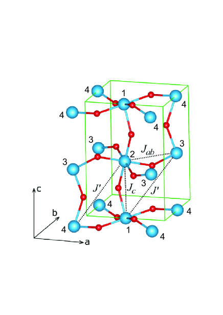
Рис. 3: (Color online) Structure of the Fe³⁺–O^2-–Fe³⁺ superexchange bonding in orthoferrites. $J_{ab}$ and $J_{c}$ are nearest-neighbor superexchange integrals, $J^{\prime}$ superexchange integral for next-nearest-neighbors. 1, 2, 3, 4, are Fe³⁺ ions in four nonequivalent positions. Reproduced from Ref. [53].

4 Theoretical predictions as compared with experiment

4.1 Dzyaloshinskii interaction in orthoferrites

Four Fe³⁺ ions occupy positions 4b in the orthorhombic elementary cell of orthoferrites RFeO₃ (space group $Pbnm$):

$$1\,(1/2,0,0);2\,(1/2,0,1/2);3\,(0,1/2,1/2);4\,(0,1/2,0)\,.$$

Classical basis vectors of magnetic structure for 3$d$ sublattice are defined as follows:

$$4S{\bf F}={\bf S}_{1}+{\bf S}_{2}+{\bf S}_{3}+{\bf S}_{4}\,;\\$$

$$4S{\bf G}={\bf S}_{1}-{\bf S}_{2}+{\bf S}_{3}-{\bf S}_{4}\,;\\$$

$$4S{\bf C}={\bf S}_{1}+{\bf S}_{2}-{\bf S}_{3}-{\bf S}_{4}\,;\\$$

$$4S{\bf A}={\bf S}_{1}-{\bf S}_{2}-{\bf S}_{3}+{\bf S}_{4}\,.$$ (38)

Here ${\bf G}$ describes the main antiferromagnetic component, ${\bf F}$ gives the weak ferromagnetic moment (overt canting), the weak antiferromagnetic components ${\bf C}$ and ${\bf A}$ describe a canting without net magnetic moment (hidden canting). Allowed spin configurations for 3$d$-sublattice are denoted as $\Gamma_{1}\,(A_{x},G_{y},C_{z})$, $\Gamma_{2}\,(F_{x},C_{y},G_{z})$, $\Gamma_{4}\,(G_{x},A_{y},F_{z})$, where the components given in parentheses are the only ones different from zero. It is worth noting that another labeling of the Fe³⁺ positions than what was used here is found in the literature (see, for example, Refs. [62, 53]), in which case the basis vectors ${\bf G}$, ${\bf C}$, ${\bf A}$ may differ in sign.

Within simplest classical approximation the operator of symmetric and antisymmetric $d$ - $d$ exchange interactions in orthoferrites

$${\hat{H}}=\sum_{i>j}J_{ij}({\bf S}_{i}\cdot{\bf S}_{j})+\sum_{i>j}({\bf d}_{ij}\cdot[{\bf S}_{i}\times{\bf S}_{j}])$$ (39)

can be written in terms of basis vectors as free energy as follows (see, e.g., Ref. [11] and references therein)

$$\Phi=\frac{J_{F}}{2}{\bf F}^{2}+\frac{J_{G}}{2}{\bf G}^{2}+\frac{J_{C}}{2}{\bf C}^{2}+\frac{J_{A}}{2}{\bf A}^{2}+$$

$$D_{x}(C_{y}G_{z}-C_{z}G_{y})+D_{y}(F_{z}G_{x}-F_{x}G_{z})+D_{z}(A_{x}G_{y}-A_{y}G_{x})$$

$$d_{x}(A_{y}F_{z}-A_{z}F_{y})+d_{y}(C_{z}A_{x}-C_{x}A_{z})+d_{z}(C_{x}F_{y}-C_{y}F_{x})\,,$$ (40)

where for the energy per ion

$$J_{F}=-J_{G}=S^{2}(2J_{ab}+J_{c});J_{A}=-J_{C}=S^{2}(2J_{ab}-J_{c});$$

$$D_{x}=-S^{2}\sum_{2}d_{x}(12);$$

$$D_{y}=-S^{2}\left(\sum_{4}d_{y}(14)+\sum_{2}d_{y}(12)\right);$$

$$D_{z}=-S^{2}\sum_{4}d_{z}(14);$$ (41)

By minimizing the free energy under condition ${\bf F}^{2}+{\bf G}^{2}+{\bf C}^{2}+{\bf A}^{2}=1$ and $F,C,A\ll G$ we find

$$F_{z}=-\frac{D_{y}}{J_{F}-J_{G}}G_{x};\,\,A_{y}=\frac{D_{z}}{J_{A}-J_{G}}G_{x};$$

$$F_{x}=\frac{D_{y}}{J_{F}-J_{G}}G_{z};\,\,C_{y}=-\frac{D_{x}}{J_{C}-J_{G}}G_{z};$$

$$A_{x}=-\frac{D_{z}}{J_{A}-J_{G}}G_{y};\,\,C_{z}=\frac{D_{x}}{J_{C}-J_{G}}G_{y};$$ (42)

4.2 Overt and hidden canting in orthoferrites

Figure 3 shows the intricate structure of the Fe³⁺–O^2-–Fe³⁺ superexchange bondings in orthoferrites that points to a complicated structural dependence of the Dzyaloshinskii vectors.

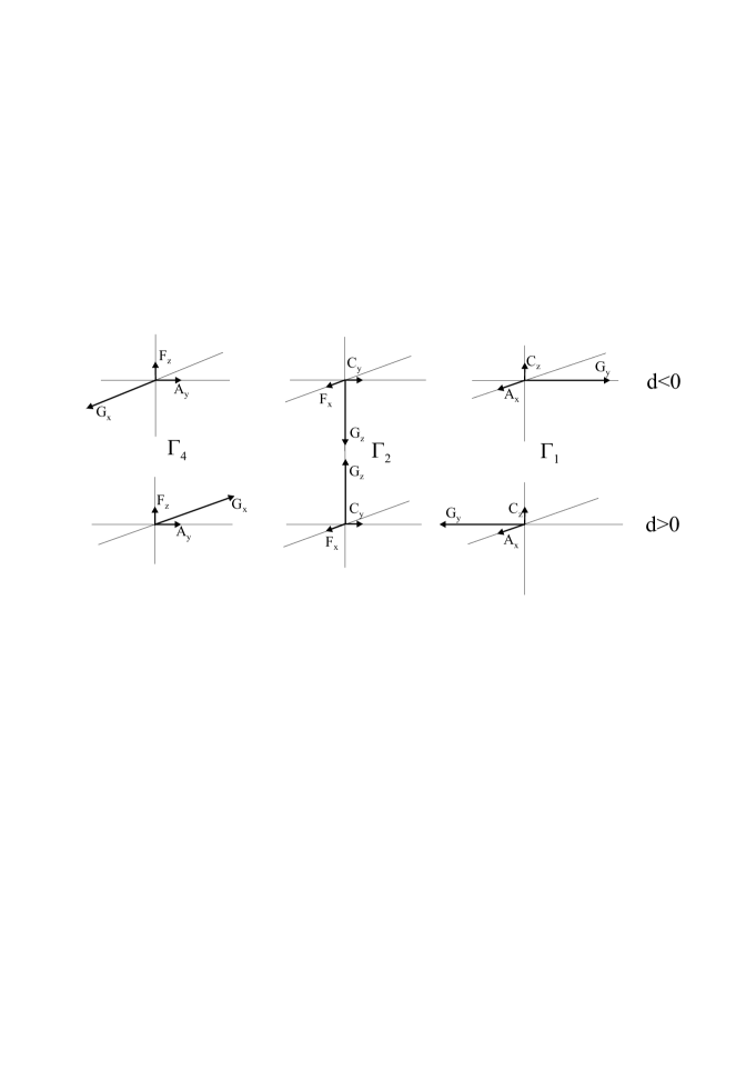
Рис. 4: Basic vectors of magnetic structure for 3$d$ sublattice in orthoferrites RFeO₃ and orthochromites RCrO₃

In Table 5 we present structural factors $\left[{\bf r}_{1}\times{\bf r}_{2}\right]_{x,y,z}$ for the superexchange coupling of the Fe³⁺ ion in position (1/2, 0, 0) with nearest neighbors in orthoferrites with numerical values for YFeO₃. It is easy to see that the weak ferromagnetism in orthoferrites governed by the $y$-component of the Dzyaloshinskii vector does actually make use of only about one-third of its maximal value.

In 1975 we made use of simple formula for the Dzyaloshinskii vector (6) and structural factors from Table 5 to find a relation between crystallographic and canted magnetic structures for four-sublattice’s orthoferrites RFeO₃ and orthochromites RCrO₃ [9, 11] (see Fig. 4), where main G-type antiferromagnetic order is accompanied by both overt canting characterized by ferromagnetic vector ${\bf F}$ (weak ferromagnetism!) and two types of a hidden canting, ${\bf A}$ and ${\bf C}$ (weak antiferromagnetism!):

$$F_{x}=\frac{(x_{1}+2z_{2})ac}{6l^{2}}\frac{d}{J}G_{z}\,;\,F_{z}=-\frac{(x_{1}+2z_{2})ac}{6l^{2}}\frac{d}{J}G_{x}\,;\,$$

$$A_{x}=\frac{(\frac{1}{2}+y_{2}-x_{2})ab}{2l^{2}}\frac{d}{J}G_{y};A_{y}=-\frac{(\frac{1}{2}+y_{2}-x_{2})ab}{2l^{2}}\frac{d}{J}G_{x};$$

$$C_{y}=\frac{(\frac{1}{2}-y_{1})bc}{2l^{2}}\frac{d}{J}G_{z}\,;\,C_{z}=-\frac{(\frac{1}{2}-y_{1})bc}{2l^{2}}\frac{d}{J}G_{y}\,,$$ (43)

where $a,b,c$ are unit cell parameters, $x_{1,2},y_{1,2},z_{2}$ are oxygen ($O_{I,II}$) parameters, $l$ is a mean cation-anion separation. These relations imply an averaging on the Fe³⁺ - O^2- - Fe³⁺ bonds in $ab$ plane and along $c$-axis. It is worth noting that $|A_{x,y}|>|F_{x,z}|>|C_{y,z}|$.

Таблица 6: Hidden canting in orthoferrites.

Orthoferrite	Ay/Fz, theory [9]	Ay/Fz, exp	Ay/Cy, theory [9]	Ay/Cy, exp
YFeO$3$	1.10	1.10 $\pm$ 0.03[22] 1.23 $\pm$ 0.2[23] 1.1 $\pm$ 0.1[63] 1.14 [52] 1.03 [53]	2.04	?
HoFeO$3$	1.16	0.85 $\pm$ 0.10[63]	2.00	?
TmFeO$3$	1.10	1.25 $\pm$ 0.05[22]	1.83	?
YbFeO$3$	1.11	1.22 $\pm$ 0.05[23]	1.79	2.0 $\pm$ 0.2[22]

First of all we arrive at a simple relation between crystallographic parameters and magnetic moment of the Fe-sublattice: in units of $G\cdot g/cm^{3}$

$$M_{Fe}=\frac{4g\mu_{B}S}{\rho V}|F_{x,z}|=\frac{2g\mu_{B}Sac}{3l^{2}\rho V}(x_{1}+2z_{2})\frac{d(\theta)}{J(\theta)}\,,$$ (44)

where $\rho$ and $V$ are the unit cell density and volume, respectively. The overt canting $F_{x,z}$ can be calculated through the ratio of the Dzyaloshinskii ($H_{D}$) and exchange ($H_{E}$) fields as follows

$$F=H_{D}/2H_{E}\,.$$ (45)

If we know the Dzyaloshinskii field we can calculate the $d(\theta)$ parameter in orthoferrites as follows

$$H_{D}=\frac{S}{g\mu_{B}}\sum_{i}|d_{y}(1i)|=\frac{S}{g\mu_{B}}(x_{1}+2z_{2})\frac{ac}{l^{2}}|d(\theta)|\,,$$ (46)

that yields $|d(\theta)|\cong$ 3.2 K = 0.28 meV in YFeO₃ given $H_{D}$ = 140 kOe [17]. This value is in good agreement with the data of recent experiments [52, 53] which make it possible to obtain information on the Dzyaloshinskii vectors based on measurements of the spin-wave spectrum. It is worth noting that despite $F_{z}\approx$ 0.01 the $d(\theta)$ parameter is only one order of magnitude smaller than the exchange integral in YFeO₃.

Our results have stimulated experimental studies of the hidden canting, or "weak antiferromagnetism"in orthoferrites. As shown in Table 6 the theoretically predicted relations between overt and hidden canting nicely agree with the experimental data obtained for different orthoferrites by NMR [22], neutron diffraction, measurement of the low-energy spin excitations by inelastic neutron scattering and by absorption of THz radiation  [23, 63, 52, 53].

4.3 The DM coupling and effective magnetic anisotropy

Hereafter we demonstrate a contribution of the DM coupling into effective magnetic anisotropy in orthoferrites. The classical energies of the three spin configurations in orthoferrites $\Gamma_{1}(A_{x},G_{y},C_{z})$, $\Gamma_{2}(F_{x},C_{y},G_{z})$, and $\Gamma_{4}(G_{x},A_{y},F_{z})$ given $|F_{x}|=|F_{z}|=F$, $|C_{y}|=|C_{z}|=C$, $|A_{x}|=|A_{z}|=A$ can be written as follows [11]

$$E_{\Gamma_{1}}=E_{G}-48JS^{2}F^{2}\left[\frac{1}{3}(\frac{C}{F})^{2}+\frac{2}{3}(\frac{A}{F})^{2}\right]\,;$$ (47)

$$E_{\Gamma_{2}}=E_{G}-48JS^{2}F^{2}\left[1+\frac{1}{3}(\frac{C}{F})^{2}\right]\,;$$ (48)

$$E_{\Gamma_{4}}=E_{G}-48JS^{2}F^{2}\left[1+\frac{2}{3}(\frac{A}{F})^{2}\right]\,,$$ (49)

with obvious relation $E_{\Gamma_{4}}<E_{\Gamma_{1}}\leq E_{\Gamma_{2}}$. The energies allow us to find the constants of the in-plane magnetic anisotropy $E_{an}=k_{1}\,cos2\theta$ ($ac$, $bc$ planes), $E_{an}=k_{1}\,cos2\varphi$ ($ab$ plane): $k_{1}(ac)=\frac{1}{2}(E_{\Gamma_{2}}-E_{\Gamma_{4}})$; $k_{1}(bc)=\frac{1}{2}(E_{\Gamma_{2}}-E_{\Gamma_{1}})$; $k_{1}(ab)=\frac{1}{2}(E_{\Gamma_{4}}-E_{\Gamma_{1}})$. Detailed analysis of different mechanisms of the magnetic anisotropy of the orthoferrites [11, 64] points to a leading contribution of the DM coupling. Indeed, for all the orthoferrites RFeO₃ this mechanism does predict a minimal energy for $\Gamma_{4}$ configuration which is actually realized as a ground state for all the orthoferrites, if one neglects the R-Fe interaction. Furthermore, predicted value of the constant of the magnetic anisotropy in $ac$-plane for YFeO₃ $k_{1}(ac)$ =2.0$\cdot 10^{5}$ erg/cm³ is close enough to experimental value of 2.5$\cdot 10^{5}$ erg/cm³ [17]. Interestingly, the model predicts a close energy for $\Gamma_{1}$ and $\Gamma_{2}$ configurations so that $|k_{1}(bc)|$ is about one order of magnitude less than $|k_{1}(ac)|$ and $|k_{1}(ab)|$ for most orthoferrites [11, 64]. It means the anisotropy in $bc$-plane will be determined by a competition of the DM coupling with relatively weak contributors such as magneto-dipole interaction and single-ion anisotropy. It should be noted that the sign and value of the $k_{1}(bc)$ is of a great importance for the determination of the type of the domain walls for orthoferrites in their basic $\Gamma_{4}$ configuration (see, e.g., Ref. [65]).

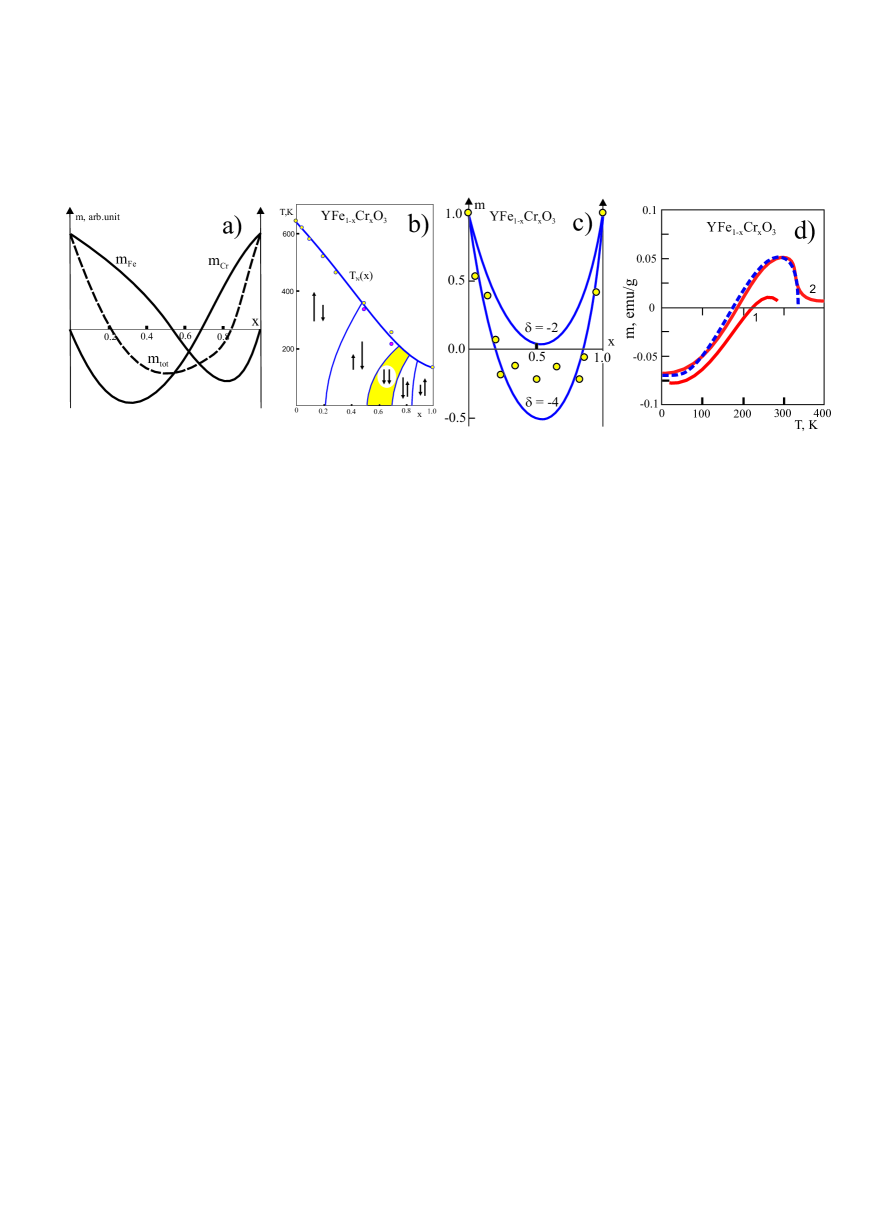
Рис. 5: (Color online) a) Concentration dependence of the magnetization and Fe-, Cr- partial contributions in YFe_0.5Cr_0.5O₃; b) The MFA phase diagram of weak ferrimagnet YFe_1-xCr_xO₃ given $\delta$ = -4; left and right arrows demonstrate the orientation and magnitude of the magnetization for Fe- and Cr-sublattices, respectively. The outer and inner thin curves mark the compensation points for the net and partial (Fe, Cr) magnetization, respectively. Experimental values of $T_{N}$ for single crystalline and polycrystalline samples are marked by light and dark circles, respectively. c) Concentration dependence of the low-temperature magnetization in YFe_1-xCr_xO₃: experimental data (circles) [21], the MFA calculations given $\delta$ = -2 and -4; c) ; d) Temperature dependence of magnetization in YFe_1-xCr_xO₃: solid curves – experimental data for x = 0.38 (Kadomtseva et al., 1977 [66] – curve 1) and for x = 0.4 (Dasari et al., 2012 [71] – curve 2), dotted curve – the MFA calculation for x = 0.4 [71] given $d_{FeCr}$ = -0.39 K

5 Weak ferrimagnetism as a novel type of magnetic ordering in systems with competing signs of the Dzyaloshinskii vector

First experimental studies of mixed orthoferrites-orthochromites YFe_1-xCr_xO₃ [21] performed in Moscow State University did confirm theoretical predictions regarding the signs of the Dzyaloshinskii vectors and revealed the weak ferrimagnetic behavior due to a competition of Fe-Fe, Cr-Cr, and Fe-Cr DM coupling with antiparallel orientation of the mean weak ferromagnetic moments of Fe and Cr subsystems in a wide concentration range. In other words, we have predicted a novel class of mixed 3$d$ systems with competing signs of the Dzyaloshinskii vector, so called weak ferrimagnets. Transversal weak ferromagnetic moment of the Cr³⁺ impurity ion in orthoferrite YFeO₃ can be evaluated as follows

$${\bf m}_{Cr}=g\mu_{B}S_{Cr}(2\delta-1){\bf F}\,,$$ (50)

where dimensionless parameter

$$\delta=\frac{d_{CrFe}}{d_{FeFe}}\frac{I_{FeFe}}{I_{CrFe}}$$ (51)

does characterize a relative magnitude of the impurity-matrix DM coupling. By comparing $m_{Cr}$ with that of the matrix value ${\bf m}_{Fe}=g\mu_{B}S_{Fe}{\bf F}$ we see that the weak ferromagnetic moment for the Cr impurity is antiparallel to that of the Fe matrix even for positive but small $\delta<1/2$. However, the effect is more pronounced for negative $\delta$, that is for different signs of $d_{CrFe}$ and $d_{FeFe}$.

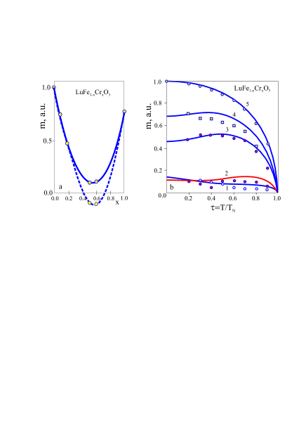
Рис. 6: (Color online) a) Concentration dependence of the low-temperature ($T$ = 77 K) magnetization in LuFe_1-xCr_xO₃: experimental data (circles) [67], the MFA calculations (solid curve) given $\delta$ = -1.5. (b) Temperature dependence of magnetization in LuFe_1-xCr_xO₃: circles – experimental data [67] given $x$ = 0.6 (1), 0.5 (2), 0.2 (3), 0.1 (4), 0.0 (5), solid curves – the MFA calculations given $\delta$ = -1.5.

Results of a simple mean-field calculation presented in Figs.5-7 show that the weak ferrimagnets such as RFe_1-xCr_xO₃, Mn_1-xNi_xCO₃, Fe_1-xCr_xBO₃ [21, 66, 67, 68, 69, 70] do reveal very nontrivial concentration and temperature dependencies of magnetization, in particular, the compensation point(s).

In Fig. 5a,b,c we do present the MFA "weak ferrimagnetic"  phase diagram, concentration dependence of the low-temperature net magnetization, and the Fe, Cr partial contributions in YFe_1-xCr_xO₃ calculated at constant value of $\delta$ = -4. Comparison with experimental data for the low-temperature net magnetization [21] and the MFA calculations with $\delta$ = -2 (Fig. 5c) points to a reasonably well agreement everywhere except $x\sim$ 0.5, where $\delta$ parameter seems to be closer to $\delta$ = -3. In Fig. 5d we compare first pioneering experimental data for the temperature dependence of magnetization $m(T)$ in weak ferrimagnet YFe_1-xCr_xO₃ ($x$ = 0.38) (Kadomtseva et al., 1978 [66] – curve 1) with recent data for a close composition with $x$ = 0.4 (Dasari et al., 2012 [71] – curve 2). It is worth noting that recent MFA calculations by Dasari et al. [71] given $d_{FeCr}$ = -0.39 K provide very nice description of $m(T)$ at $x$ = 0.4. Note that the authors [71] found a rather strong dependence of the $d_{FeCr}$ parameter on the concentration $x$. The concentration and temperature dependencies of magnetization in LuFe_1-xCr_xO₃ are nicely described by a simple MFA model under the assumption of constant sign magnetization given constant value of $\delta$ = -1.5 (Fig. 6a,b [67]), which, strictly speaking, did not exclude the possibility of an alternative description of the dependence $m(x)$ with two points of concentration compensation of magnetization (see dotted line in Fig. 6a). Furthermore, strictly speaking, the absence of compensation concentration points for low-temperature magnetization $m(x,T=77K)$ does not mean the absence of compensation points at higher temperatures. Indeed, much later, in 2016, Pomiro et al. [72] observed the spontaneous magnetization reversal in polycrystalline LuFe_0.5Cr_0.5O₃ below T_N = 290 K at a compensation temperature T_comp = 224 K and Billoni et al. [73] have performed more advanced classical Monte Carlo simulations for RFe_1-xCr_xO₃ with R = Y and Lu, comparing the numerical simulations with experiments and MFA calculations. In addition to the dependence T${}_{N}(x)$, this model is able to reproduce the magnetization reversal (MR) observed experimentally in a field cooling process for intermediate $x$ values.

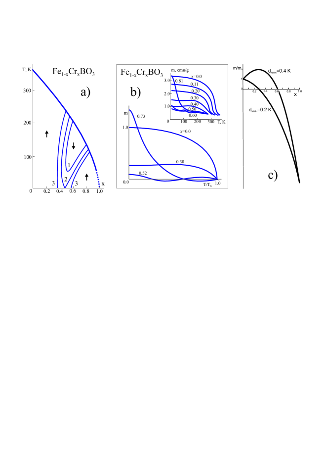
Рис. 7: a) The MFA simulation of the T-x-phase diagram of the weak ferro(ferri)magnet Fe_1-xCr_xBO₃ [68] given $I_{FeFe}=I_{FeCr}$= -20.3 K, $I_{CrCr}$ = 2.0 K, arrows point to orientation of the net weak ferromagnetic moment. Curves 1, 2, 3 mark the compensation points given $d_{z}(FeFe)$ = $d_{z}(CrCr)$ = 0.67 K, $d_{z}(FeCr)$ = -0.67 K (1), -0.75 K (2), -0.90 K (3), respectively. b) The MFA simulation of the temperature dependence of the net magnetization in Fe_1-xCr_xBO₃ [68] given $d_{z}(FeFe)$ = $d_{z}(CrCr)$ = -$d_{z}(FeCr)$ = 0.67 K at different compositions, the insert shows experimental data from Ref. [77] taken at external magnetic field 1 T. c) The MFA simulation of the concentration dependence of the low-temperature magnetization in Mn_1-xNi_xCO₃ [70] given $d_{z}(MnNi)>d_{z}^{(0)}(MnNi)$ and $d_{z}(MnNi)<d_{z}^{(0)}(MnNi)$, respectively.

At variance with YFeO₃ and YCrO₃ which are weak ferromagnets with main G_xF_z-type magnetic structure below T_N, the orthoferrites-orthochromites YFe_1-xCr_xO₃, which referred as weak ferrimagnets, reveal full or partial G_xF_z– G_zF_x type spin-reorientation in a wide range of substitution. This unexpected behavior which is usually typical for orthoferrites with magnetic rare-earth ions (Er, Tm, Dy,…) was attributed mainly to a strong decrease of the DM contribution to magnetic anisotropy in the $ac$-plane for $x$ = 0.5–0.6 [74, 75]. In contrast to the yttrium system, the lutetium orthoferrite-orthocromites LuFe_1-xCr_xO₃ (x = 0.0, 0.1, 0.2, 0.5, 0.6, and 1.0) reveal the main G_xF_z type magnetic structure without signatures of the spontaneous spin-reorientation transition. This difference can be explained by the significantly larger contribution of single-ion anisotropy to $k_{ac}$ in LuFeO₃ as compared to YFeO₃ [11, 76].

Let us turn to the features of other weak ferrimagnets. Fig. 7b shows a calculated phase diagram of the trigonal weak ferrimagnet Fe_1-xCr_xBO₃ [68]. Temperature-dependent magnetization studies from 4.2 to 600 K have been made for the solid solution system Fe_1-xCr_xBO₃ where $0\leq x\leq$ 95 [77]. A rapid decrease is observed in the saturation magnetization with increasing $x$ at 4.2 K up to 0.40, after which a broad compositional minimum is found up to x=0.60. Compositions in the range of 0.40$\leq x\leq$0.60 display unusual magnetization behavior as a function of temperature in that maxima and minima are present in the curves below the Curie temperatures. Fig. 7b shows a nice agreement between experimental data [77] and our MFA calculations.

At variance with the $d^{5}$ - $d^{3}$ (Fe-Cr) mixed systems such as YFe_1-xCr_xO₃ or Fe_1-xCr_xBO₃ the manifestation of different DM couplings Fe-Fe, Cr-Cr, and Fe-Cr in (Fe_1-xCr_x)₂O₃ is all the more surprising because of different magnetic structures of the end compositions, $\alpha$-Fe₂O₃ and Cr₂O₃ and emergence of a nonzero DM coupling for the three-corner-shared FeO₆ and CrO₆ octahedra, "forbidden"  for Fe-Fe and Cr-Cr bonding. All this makes magnetic properties of mixed compositions (Fe_1-xCr_x)₂O₃ to be very unusual [78].

Unlike the $d^{5}$ - $d^{3}$ (Fe-Cr) mixed systems YFe_1-xCr_xO₃ or Fe_1-xCr_xBO₃, where the two concentration compensation points do occur given rather large $d_{FeCr}$ parameter, in the $d^{5}$ - $d^{8}$ systems, the nickel and fluorine substituted orthoferrites RFe_1-xNi_xF_yO_3-y [69] or Mn_1-xNi_xCO₃ with Mn²⁺ - Ni²⁺ pairs [70] we have the only concentration compensation point irrespective of the $d_{MnNi}$ parameter. However, the character of the concentration dependence of the weak ferrimagnetic moment $m(x)$ depends strongly on its magnitude. Given the increasing concentration the $m(x)$ is first rising or falling with $x$ depending on whether $d_{MnNi}$ greater than, or less than $d_{MnNi}^{(0)}=(1+\frac{S_{Mn}}{S_{Ni}})\frac{I_{MnNi}}{2I_{MnMn}}d_{MnMn}$. Figure (7c) does clearly demonstrate this feature.

It should be noted that just recently Dmitrienko et al. [79] have first discovered experimentally that in accordance with our theory (see Table 4) the sign of the Dzyaloshinskii vector in MnCO₃ ($d^{5}$ - $d^{5}$) coincides with that one in FeBO₃ ($d^{5}$ - $d^{5}$) , whereas NiCO₃ ($d^{8}$ - $d^{8}$) demonstrates the opposite sign.

5.1 Features of the 4$f$ - 3$d$ interaction in weak ferrimagnets RFe_1-xCr_xO₃

It is undoubtedly of interest to investigate the influence of the weak ferrimagnetic ordering of the 3$d$-sublattice on the behavior of the rare-earth subsystem in mixed ferrites-chromites RFe_1-xCr_xO₃. The character of polarization of the R-ions and its concentration and temperature dependencies yield valuable information not only on the state of the $d$-subsystem, but also on the 4$f$ - 3$d$ interaction mechanisms, primarily on the relative roles of the ferro- and antiferromagnetic contributions to the effective field at the R-ions [61, 80, 75, 81]. Of particular interest, in our opinion, is the GdFe_1-xCr_xO₃ system with $S$-type 4$f$- and 3$d$-ions, where it might seem that it is precisely the ferromagnetic contribution due to the isotropic 4$f$ - 3$d$ exchange should play the decisive role in the polarization of the Gd sublattice. At the same time, a detailed analysis of the magnetic properties of GdFeO₃ and GdCrO₃ [60, 61] has quite unexpectedly revealed the substantial role of the anisotropic exchange of the $S$-ions Gd³⁺ with $S$-type ions Fe³⁺ and Cr³⁺ and accordingly of the antiferromagnetic contribution to the polarization of the Gd sublattices with the predominance of antisymmetric term which is determined by the 4$f$ - 3$d$ DM coupling (see (36) and (37)).

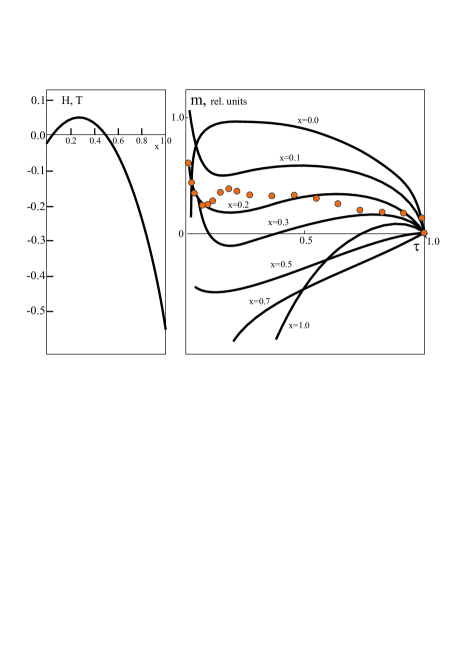
Рис. 8: (Color online) Left panel: Calculated concentration dependence of the average effective field on the Gd³⁺ ions in the weak ferrimagnet at T = 0 K. Right panel: Calculated temperature dependencies of the spontaneous magnetization for a number of weak ferrimagnets GdFe_1-xCr_xO₃ and end compositions, $\tau$ = T/T_N. Solid circles are experimental data for single crystals GdFe_0.83Cr_0.17O₃ with T_N = 550 K [61].

Knowledge of the numerical values of the parameters of isotropic and anisotropic 4$f$ - 3$d$ interaction has enabled us to calculate, within the framework of the molecular-field theory, the concentration and temperature dependencies of the average effective field $H_{z}$, the magnetization of the Gd sublattice, and the total magnetization of GdFe_1-xCr_xO₃ in the entire range of concentrations $x$ (see Fig.8) [61]. The exchange integrals and the DM coupling parameters in the $d$ sublattices were chosen equal to the corresponding values for weak ferrimagnet YFe_1-xCr_xO₃. The concentration dependence $H_{z}(x)$ at T = 0 K has very unusual form with two compensation points, at small and relatively large concentrations of the Cr³⁺ ions. Whereas at $x\approx$ 0.05 the compensation of the total magnetic moment is still observed, at $x$ = 0.10 the reversal of the sign of $H_{z}$ leads to a hyperbolic increase of $m(T)$ in the low-temperature region. At the same time the calculation shows that at $x\approx$ 0.27 and $\tau\approx$ 0.17 we arrive at the compensation point, which then "bifurcates"with one (high-temperature) compensation point moving towards T_N, with increasing $x$, while the other (low temperature) towards T = 0 K. At $x$ > 0.5 the compensation points vanish. Only for compositions directly adjacent to pure gadolinium orthochromite is the compensation again observed, and with increasing concentration of the Fe³⁺ ions the compensation point shifts from T_comp = 110 K in pure GdCrO₃, to T_comp =T_N, at $x\approx$ 0.95. As a whole the calculated concentration and temperature dependencies of the magnetization in GdFe_1-xCr_xO₃ agree satisfactorily with the experimental data [61]. Finally, we note the need for further experimental investigation of the rare-earth weak ferrimagnets such as GdFe_1-xCr_xO₃ both from the viewpoint of studying various $f$ - $d$ interactions, and of the possibility of obtaining novel advanced magnetic properties.

5.2 Unconventional spin-reorientation in weak ferrimagnets

The contribution of the competing antisymmetric exchange to the magnetic anisotropy of weak ferrimagnets has an unusual concentration dependence. So, if in pure orthoferrite YFeO₃ and orthochromite YCrO₃ antisymmetric exchange makes a decisive contribution to the stabilization of the magnetic configuration $\Gamma_{4}$, then in a weak ferrimagnet YFe_1-xCr_xO₃ it can induce a spin-reorientation $\Gamma_{4}$ – $\Gamma_{2}$ transition which are typical for several orthoferrites RFeO₃ with magnetic rare-earth ions (R = Nd, Sm, Tb, Ho, Er, Tm, Yb). In Fig. 9 we demonstrate concentration dependence of the DM coupling contribution to first anisotropy constant for YFe_1-xCr_xO₃ in $ac$-plane given different values of the parameter $\delta$, which was calculated within simple mean-field approximation [74, 75] in the limit of low temperatures. A characteristic feature of this dependence is the appearance of several extrema with a sharp decrease in the contribution in the region of intermediate concentrations near $x$ $\sim$ 0.6 - 0.7. Furthermore, similarly magnetization, this contribution to anisotropy has a specific temperature dependence [74, 75]. On the whole, both effects can lead to the appearance of spontaneous spin-reorientation transitions in weak ferrimagnets of the YFe_1-xCr_xO₃ type with a nonmagnetic "Rion. Indeed, in full accordance with the theory, such transitions have been observed experimentally, for example, the $\Gamma_{4}$ – $\Gamma_{2}$ spin-reorientation transition in YFe_0.85Cr_0.15O₃ [74, 75] (see Fig.  9).

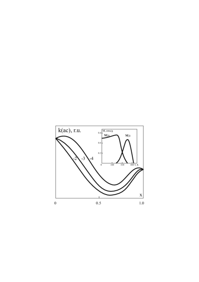
Рис. 9: Concentration dependence of the DM coupling contribution to the first anisotropy constant in $ac$-plane given different values of the parameter $\delta$. Inset: Temperature dependence of the magnetization in the weak ferrimagnet YFe_0.85Cr_0.15O₃ [75] demonstrating the $\Gamma_{4}$ – $\Gamma_{2}$ spin-reorientation transition in the temperature range 240 - 400 K.

A more surprising situation was found in the weak ferrimagnet DyFe_1-xCr_xO₃ at a relatively low concentration of Cr ions. The Dy³⁺ ions in DyFeO₃ stabilize the $\Gamma_{1}(G_{y})$ configuration, so that at T = 40 K, a jump-like Morin transition $\Gamma_{4}$ – $\Gamma_{1}$ is observed. In all single crystals of weak ferrimagnets DyFe_1-xCr_xO₃ ($x$ = 0.07, 0.10, 0.13, 0.15, 0.36, 0.40) synthesized and studied in the laboratory of A. M. Kadomtseva (Moscow State University) [74, 75], the Morin $\Gamma_{4}$ – $\Gamma_{1}$ spin-reorientation transition to the low-temperature phase $\Gamma_{1}$ was detected, with the exception of the composition with $x$ = 0.36, where the phase $\Gamma_{2}$ was unexpectedly found to be the high-temperature phase. Puzzlingly, in compositions $x$ = 0.1 and $x$ = 0.13, the Morin transition proceeded according to the $\Gamma_{4}$ – $\Gamma_{421}$ – $\Gamma_{21}$ – $\Gamma_{1}$ ($x$ = 0.1) or $\Gamma_{4}$ – $\Gamma_{421}$ – $\Gamma_{1}$ ($x$ = 0.1) scheme and was accompanied by the deviation of the antiferromagnetic vector ${\bf G}$ into space with the appearance in a narrow temperature range of the projection of the magnetic moment on the $b$-axis. Never before has the state of the mixed configuration $\Gamma_{421}(G_{x}G_{y}G_{z})$ with the spatial orientation of the antiferromagnetism vector and the appearance of the $b$-component of the magnetic moment ($M_{b}\propto G_{x}G_{y}G_{z}$) been observed.

5.3 Recent renewal of interest to weak ferrimagnets

The systems with competing antisymmetric exchange were extensively investigated up to the end of 80ths mainly in the laboratory of A. M. Kadomtseva at Moscow State University. Recent renewal of interest to the systems with the compensation point was stimulated by the perspectives of the applications in magnetic memory (see, e.g., Refs. [82, 71] and references therein). For instance, weak ferrimagnet YFe_0.5Cr_0.5O₃ exhibits magnetization reversal at low applied fields. Below a compensation temperature (T_comp), a tunable bipolar switching of magnetization is demonstrated by changing the magnitude of the field while keeping it in the same direction. The compound also displays both normal and inverse magnetocaloric effects above and below 260 K, respectively. These phenomena coexisting in a single magnetic system can be tuned in a predictable manner and have potential applications in electromagnetic devices [82]. Weak ferrimagnets can exhibit the tunable exchange bias (EB) effect [83]. Recently the EB effect with reversal sign was found in LuFe_0.5Cr_0.5O₃ ferrite-chromite [84] which is a weak ferrimagnet below T_N = 265 K, exhibiting antiparallel orientation of the mean weak ferromagnetic moments of the Fe and Cr sublattices due to opposite sign of the Fe - Cr Dzyaloshinskii vector as compared to that of the Fe - Fe and Cr - Cr. The weak FM moments of the studied compound compensate each other at temperature T_comp = 230 K, leading to the net magnetic moment reversal and to observed negative magnetization, at moderate applied field, below T_comp. Variety of such extraordinary properties as high compensation temperature, temperature-controlled positive/negative EB below/above T_comp, and switching the magnetization direction to the opposite one by magnetic field without of changing its polarity makes weak ferrimagnet LuFe_0.5Cr_0.5O₃ of promising candidate for application in magnetic memories.

Combining magnetization reversal effect with magnetoelectronics can exploit tremendous technological potential for device applications, for example, thermally assisted magnetic random access memories, thermomagnetic switches and other multifunctional devices, in a preselected and convenient manner. Nowadays a large body of magnetic materials might be addressed as systems with competing antisymmetric exchange [85], including novel class of mixed helimagnetic B20 alloys such as Mn_1-xFe_xGe where the helical nature of the main ferromagnetic spin structure is determined by a competition of the DM couplings Mn - Mn, Fe - Fe, and Mn - Fe. Interestingly, that the magnetic chirality in the mixed compound changes its sign at $x_{cr}\approx$ 0.75, probably due to different sign of the Dzyaloshinskii vectors for Mn - Mn and Fe - Fe pairs [86].

6 Determination of the sign of the Dzyaloshinskii vector

Determining the sign of the Dzyaloshinskii vector and the relative orientation of the ${\bf F}$ and ${\bf G}$ vectors in weak ferromagnets is of both fundamental importance from the standpoint of the microscopic theory of the DM coupling and practical importance for the reliable identification of the parameters of various anisotropic interactions in these materials. In particular, for the rare-earth orthoferrites RFeO₃, this concerns the parameters of the 4$f$ - 3$d$ interaction [60], the parameters of transferred and supertransferred hyperfine interactions [87], and the magnitude of the effective magnetic field for $\mu$-mesons [62]. The sign of the Dzyaloshinskii vector determines the handedness of spin helix in crystals with the noncentrosymmetric B20 structure.

How to measure the sign of the DM interaction in weak ferromagnets? According to Ref. [19], an answer to this question can be given by determining experimentally the direction of rotation of the antiferromagnetism vector ${\bf l}$ around the magnetic field ${\bf H}$ in the geometry ${\bf H}\parallel{\bf d}\parallel$easy axis. However, as was pointed out later (see Ref. [88]), a Mössbauer experiment on easy-axis hematite did not give an unambiguous result.

According to Dmitrienko et al. [89], first of all, a strong enough magnetic field should be applied to obtain the single domain state where the DM coupling pins antiferromagnetic ordering to the crystal lattice. Next, single crystal diffraction methods sensitive both to oxygen coordinates and to the phase of antiferromagnetic ordering should be used. In other words, one should observe those Bragg reflections $hkl$ where interference between magnetic scattering on Mn atoms and nonmagnetic scattering on oxygen atoms is significant. There are three suitable techniques: neutron diffraction, Mössbauer $\gamma$-ray diffraction, and resonant x-ray scattering. The sign of the DM vector in weak ferromagnetic FeBO₃ was deduced from observed interference between resonant X-ray scattering and magnetic X-ray scattering [89].

The authors in Ref. [88] claimed that the character of the field-induced transition from an antiferromagnetic phase to a canted phase in cobalt fluoride CoF₂ is due to the "sign"of the Dzyaloshinskii interaction, and this affords an opportunity to determine experimentally the sign of the Dzyaloshinskii vector. However, in fact they addressed a symmetric Dzyaloshinskii interaction that is magnetic anisotropy

$$V_{sym}=-D(m_{x}l_{y}+m_{y}l_{x})$$

rather than antisymmetric DM coupling.

In our opinion, the most reliable experimental method for determining the mutual orientation of the vectors of ferromagnetism ${\bf F}$ and antiferromagnetism ${\bf G}$, and hence the sign of the Dzyaloshinskii vector, is to study the magnitude and sign of the effective magnetic field on ligands, as well as $\mu$-mesons in weak ferromagnets.

6.1 Positive muons in orthoferrites as a tool to examine the sign of Dzyaloshinskii vector

In muon spin rotation ($\mu$SR) experiments, spin-polarized positive (anti)muons are used to probe the microscopic field distribution at the interstitial site(s) where the $\mu^{+}$ stop inside the sample under investigation. The extreme sensitivity of the muon to small magnetic fields as well as the absence of quadrupolar coupling makes this technique very promising in probing magnetic orders, offering a valuable alternative to neutron scattering. This approach, which shares many similarities with nuclear magnetic resonance, has the advantage of being applicable to virtually any material, but it has the drawback that the interstitial sites where the muon stops and the nature of muon interaction with the host are generally unknown [90]. Site assignment is the key initial ingredient in the not infrequent cases where the internal magnetic field is dominated by the distant dipole contribution, which requires only the knowledge of the site in order to be computed by a classical sum over the dipole moments of the host lattice. Thus, the comparison between predicted and measured local field can validate the muon site assignment, and in turn, this assessment yields, e.g., a measure of the magnetic moment values. However, additional local field contributions exist and these are not negligible in many cases [91].

The dipolar field can be approximated with good accuracy, assuming a classical moment ${\bf M}$ centered at the atomic positions of the magnetic atoms, and evaluating the total contribution as

$${\bf H}({\bf r}_{\mu})=\sum_{j}\left(\frac{3{\bf r}_{\mu j}({\bf M}_{j}\cdot{\bf r}_{\mu j})}{r_{\mu j}^{5}}-\frac{{\bf M}_{j}}{r_{\mu j}^{3}}\right)\,,$$ (52)

where ${\bf r}_{\mu}$ is the muon position, ${\bf M}_{j}$ is the magnetic moment of $j$-th ion, ${r_{\mu j}}$ is the distance between $j$-th ion and the muon site. The hyperfine Fermi contact field contribution, transferred or supertransferred, can be written as follows

$$H({\bf r}_{\mu})=\frac{8\pi}{3}\mu_{B}\rho_{s}({\bf r}_{\mu})\,,$$ (53)

where $\rho_{s}$ is the spin density at the muon site [91].

First detailed investigation of positive muons in orthoferrites RFeO₃ (R= Sm, Eu, Dy, Ho, Y, Er) has been performed by Holzschuh et al. [62]. In their presentation the hyperfine field at the muon site in the orthoferrites can be explained in terms of dipolar fields only. By comparing measured internal magnetic fields with calculated dipolar fields of Fe³⁺ ions the authors found the position of stable muon site, furthermore, they established that in configuration $\Gamma_{4}$ the sign of $G_{x}$ should be positive for $F_{z}>0$, in accordance with our earlier theoretical predictions [10], since only this assumption leads to a reasonable muon site.

However, these results were severely criticized in work [92], the authors of which argued that the interpretation [62] contains some serious flaws: important details have not been worked out correctly and their analysis is not complete enough to support some of their conclusions. First of all it concerns the supertransferred hyperfine field contribution, which must not be disregarded. Furthermore, they drew attention to the need for strict accounting of the sign convention, labeling of the Fe³⁺ ions and the representation of the spin configurations which is not uniform in the literature. This all casts doubt in using theoretical relations, in particular, concerning the mutual orientation of the ferro- and antiferromagnetic vectors, that is, in fact, the sign of the Dzyaloshinskii vector.

6.2 The ligand NMR in weak ferromagnets and first reliable determination of the sign of the Dzyaloshinskii vector

As was firstly shown in our paper [20] reliable local information on the sign of the Dzyaloshinskii vector, or to be exact, that of the Dzyaloshinskii parameter $d_{12}$, can be extracted from the ligand NMR data in weak ferromagnets. The procedure was described in details for ¹⁹F NMR data in weak ferromagnet FeF₃ [20].

The F^- ions in the unit cell of FeF₃ occupy the six positions [93]. In a trigonal basis these are $\pm(x,1/2-x,1/4),\quad\pm(1/2-x,1/4,x),\pm(1/4,x,1/2-x)$, that correspond to i) $\pm(3p(x-1/4),\sqrt{3}p(1/4-x),c/4)$, ii) $\pm(3p(1/4-x),\sqrt{3}p(1/4-x),c/4)$, and iii) $\pm(0,2\sqrt{3}p(x-1/4),c/4)$ in an orthogonal basis with $O_{z}\parallel C_{3}$ and $O_{x}\parallel C_{2}$. Each F^- ion is surrounded by two Fe³⁺ from different magnetic sublattices. Hereafter we introduce basic ferromagnetic F and antiferromagnetic G vectors:

$$2S{\bf F}={\bf S_{1}}+{\bf S_{2}},2S{\bf G}={\bf S_{1}}-{\bf S_{2}},{\bf F^{2}}+{\bf G^{2}}=1,$$ (54)

where Fe${}_{1}^{3+}$ and Fe${}^{3+}_{2}$ occupy positions (1/2,1/2,1/2) and (0,0,0), respectively. FeF₃ is an easy plane weak ferromagnet with F and G lying in (111) plane with ${\bf F}\bot{\bf G}$. The two possible variants of the mutual orientation of the F and G vectors in the basis plane, tentatively called as "left"and "right respectively, are shown in Fig. 10. The DM energy per Fe³⁺ - F^- - Fe³⁺ bond can be written as follows

$$E_{DM}=-2S^{2}d_{z}(12)(F_{x}G_{y}-F_{y}G_{x})=$$

$$-\frac{4\sqrt{3}}{l^{2}}p^{2}(x+\frac{1}{4})d(\theta)=+0.78S^{2}d(\theta)(F_{x}G_{y}-F_{y}G_{x})\,.$$ (55)

In other words, the "left"and "right"orientations of basic vectors are realized at $d(\theta)<0$ and $d(\theta)>0$, respectively.

Absolute magnitude of the ferromagnetic vector is numerically equals to an overt canting angle which can be found making use of familiar values of the Dzyaloshinskii field: $H_{D}=48.8$ kOe and exchange field: $H_{E}=4.4\cdot 10^{3}$ kOe [16] as follows

$$F=H_{D}/2H_{E}\simeq 5.5\cdot 10^{-3}.$$ (56)

If we know the Dzyaloshinskii field we can calculate the $d(\theta)$ parameter as follows

$$H_{D}=\frac{6S}{g\mu_{B}}|d_{z}(12)|=\frac{6S}{g\mu_{B}}0.39|d(\theta)|=48.8\,kOe\,,$$ (57)

that yields $|d(\theta)|\cong$ 1.1 K that is three times smaller than in YFeO₃.

Рис. 10: Two mutual orientations of $\bf F$ and $\bf G$ vectors in basal plane of FeF₃.

The local field on the nucleus of the nonmagnetic F^- anion in weak ferromagnet FeF₃, induced by neighboring magnetic $S$-type ion (Fe³⁺, Mn³⁺,…) can be written as follows [94]

$${\bf H}=-\frac{1}{\gamma_{n}}\hat{A}{\bf S}$$ (58)

($\gamma_{n}$ is a gyromagnetic ratio, $\gamma_{n}$=4.011 MHz/kOe, ${\bf S}$ is the spin moment of the magnetic ion), where the tensor of the transferred hyperfine interactions (HFI) $\hat{A}$ consists of two terms: i) an isotropic contact term with $A_{ij}=A_{s}\delta_{ij}$

$$A_{s}=\frac{f_{s}}{2S}A^{(0)}_{s},\qquad A^{(0)}_{s}=\frac{16}{3}\pi\mu_{B}\gamma_{n}|\varphi_{2s}(0)|^{2}\,;$$ (59)

ii) anisotropic term with

$$A_{ij}=A_{p}(3n_{i}n_{j}-\delta_{ij}),$$ (60)

where ${\bf n}$ is a unit vector along the nucleus-magnetic ion bond and the $A_{p}$ parameter includes the dipole and covalent contributions

$$A_{p}=A_{p}^{cov}+A_{d},$$ (61)

$$A_{p}^{cov}=\frac{(f_{\sigma}-f_{\pi})}{2S}A_{p}^{(0)},A_{p}^{(0)}=\frac{4}{5}\mu_{B}\gamma_{n}\langle\frac{1}{r^{3}}\rangle_{2p},$$

$$A_{d}=\frac{g_{s}\mu_{B}\gamma_{n}}{R^{3}}.$$ (62)

Here $f_{s,\pi,\sigma}$ are parameters for the spin density transfer: magnetic ion - ligand along the proper $s-,\sigma-,\pi$-bond [95]; $|\varphi_{2s}(0)|^{2}$ is a probability density of the $2s$-electron on nucleus; $\langle\frac{1}{r^{3}}\rangle_{2p}$ is a radial average.

The transferred HFI for ¹⁹F in fluorides are extensively studied by different techniques, NMR, ESR, and ENDOR [94]. For ¹⁹F one observes large values both of $A_{s}^{(0)}$ and $A_{p}^{(0)}$; $A_{s}^{(0)}=4.54\cdot\leavevmode\nobreak\ 10^{4}$, $A_{p}^{(0)}=1.28\cdot\leavevmode\nobreak\ 10^{3}$ MHz [94], together with the 100% abundance, nuclear spin $I=1/2$, and large gyromagnetic ratio this makes the study of the transferred HFI to be simple and available one.

Contribution of the isotropic and anisotropic transferred HFI to the local field on the ¹⁹F can be written as follows

$${\bf H}(iso)=-\frac{2S}{\gamma_{n}}A_{s}{\bf F}=a_{F}{\bf F},$$

$${\bf H}(an)={\bf\stackrel{{\scriptstyle\leftrightarrow}}{{a}}}{\bf G},\hat{a}=-\frac{2S}{\gamma_{n}}({\bf\stackrel{{\scriptstyle\leftrightarrow}}{{A}}}(1)-{\bf\stackrel{{\scriptstyle\leftrightarrow}}{{A}}}(2)).$$ (63)

The $A_{s}$ and $A_{p}$ parameters we need to calculate parameter $a_{F}$ and the HFI anisotropy tensor ${\bf\stackrel{{\scriptstyle\leftrightarrow}}{{a}}}$ that is to calculate the "ferro-"and "antiferro-"contributions to $H$ one can find in the literature data for the pair ¹⁹F - Fe³⁺. For instance, in KMgF₃:Fe³⁺ ($R_{MgF}$ = 1.987Å) [96] $A_{s}=+72,A_{p}=+18$ MHz, in K₂NaFeF₆ ($R_{FeF}$ = 1.91Å), in K₂NaAlF₆:Fe³⁺ $A_{s}$ = +70.17, $A_{p}$ = +20.34 MHz [97]. Thus, we expect in FeF₃ $|a_{F}|\sim 350\div 360$ MHz $(a_{F}<0)$ and $H(iso)\simeq 2$ MHz ($\simeq 0.5$ kOe).

In the absence of an external magnetic field the NMR frequencies for ¹⁹F in positions 1,2,3 can be written as follows

$$\nu^{2}=\gamma_{n}^{2}[(\hat{a}{\bf G})^{2}+(a_{f}{\bf F})^{2}+2a_{F}{\bf F}\hat{a}{\bf G}]=$$

$$\gamma_{n}^{2}(a_{xy}^{2}+a_{F}^{2}F^{2}\pm 2a_{F}a_{xy}F)+$$

$$\gamma_{n}^{2}(a_{yz}^{2}\mp 4a_{F}a_{xy}F)\left\{\parbox{85.35826pt}{$\cos^{2}\varphi\\ \cos^{2}(\varphi+60^{o})\\ \cos^{2}(\varphi-60^{o})$}\right.$$ (64)

where the $a_{xy},a_{yz}$ components are taken for ¹⁹F in position 1; $\varphi$ is an azimuthal angle for ferromagnetic vector F in basis plane. The formula (64) does provide a direct linkage between the ¹⁹F NMR frequencies and parameters of the crystalline $(p,c,x,l)$ and magnetic $(F,\varphi,\pm)$ structures. As of particular importance one should note a specific dependence of the ¹⁹F NMR frequencies on mutual orientation of the ferro- and antiferromagnetic vectors or the sign of the Dzyaloshinskii vector: upper signs in (64) correspond to "right orientation"  ($d(\theta)$ > 0) while lower signs do to "left orientation"  ($d(\theta)$ < 0) as shown in Fig. 10.

Рис. 11: (Color online) Comparison of simulated (upper panels) and experimental (bottom panel) zero-field ¹⁹F NMR spectra in FeF₃.

For minimal and maximal values of the ¹⁹F NMR frequencies we have

$${}\nu^{\pm}_{min}=\gamma_{n}[a_{xy}^{2}+a_{F}^{2}\pm 2a_{F}a_{xy}F]^{1/2},$$

$$\nu^{\pm}_{max}=\gamma_{n}[a_{xy}^{2}+a_{yz}^{2}+a_{F}^{2}F^{2}\mp 2a_{F}a_{xy}F]^{1/2}.$$ (65)

Taking into account the smallness of isotropic HFI contribution, signs of $a_{F}$ and $A_{xy}$ we arrive at estimations

$$\nu^{\pm}_{min}\simeq\gamma_{n}(|a_{xy}|\mp|a_{F}F|)=2.92A_{p}\mp|a_{F}F|,$$

$$\nu^{\pm}_{max}\simeq\gamma_{n}\left([a_{xy}^{2}+a_{yz}^{2}]^{1/2}\pm\frac{|a_{xy}}{[a_{xy}^{2}+a_{yz}^{2}]^{1/2}}|a_{F}F|\right)=$$

$$3.65A_{p}\pm 0.8|a_{F}F|.$$ (66)

Thus

$$(\nu_{max}-\nu_{min})^{\pm}=0.68A_{p}\pm 1.8|a_{F}F|.$$ (67)

By using the $A_{s}$ and $A_{p}$ values, typical for ¹⁹F –Fe³⁺ bonds [96, 97] we get (in MHz)

$$\nu^{+}_{min}=57.6,\nu^{+}{max}=75.7,(\nu_{max}-\nu_{min})^{+}=18.1$$ (68)

given "right hand side orientation"of F and G (Fig. 10) and

$$\nu^{-}_{min}=61.4,\nu^{-}_{max}=72.7,(\nu_{max}-\nu_{min})^{-}=11.3$$ (69)

given "left hand side orientation"of F and G (Fig. 10) .

The zero-field ¹⁹F NMR spectrum for single-crystalline samples of FeF₃ we simulated on assumption of negligibly small in-plane anisotropy [98] is shown in Fig. 11 for two different mutual orientations of ${\bf F}$ and ${\bf G}$ vectors. For a comparison in Fig. 11 we adduce the experimental NMR spectra for polycrystalline samples of FeF₃ [99, 100], which are characterized by the same boundary frequencies despite rather varied shape. Obviously, the theoretically simulated NMR spectrum does nicely agree with the experimental ones only for "right"mutual orientations of ${\bf F}$ and ${\bf G}$ vectors, or $d(FeFe)$ > 0, in a full accordance with our theoretical sign predictions (see Table 4).

The same result, $d(FeFe)$ > 0 follows from the the magnetic $x$-ray scattering amplitude measurements in the weak ferromagnet FeBO₃ [89].

6.3 The sign of the Dzyaloshinskii vector in FeBO₃ and $\alpha$-Fe₂O₃

Making use of structural data for FeBO₃ [101] we can calculate the $z$-component of the Dzyaloshinskii vector for Fe₁-O-Fe₂ pair, with Fe_1,2 in positions (1/2,1/2,1/2), (0,0,0), respectively, as follows:

$$d_{z}(12)=d_{12}(\theta)\left[{\bf r}_{1}\times{\bf r}_{2}\right]_{z}=+\frac{1}{3}(\frac{1}{2}-x_{h})\frac{ab}{l^{2}}d_{12}(\theta)$$

$$\approx+0.61\,d_{12}(\theta)\,,$$ (70)

where $a$ = 4.626 Å, $b$ = 8.012 Å  are parameters of the orthohexagonal unit cell, $x_{h}$ = 0.2981 oxygen parameter, $l$ = 2.028 Å  is a mean Fe-O separation [101].

Similarly to FeF₃ the DM energy per Fe³⁺ - O^2- - Fe³⁺ bond can be written as follows

$$E_{DM}=d_{z}(12)\left[{\bf S}_{1}\times{\bf S}_{2}\right]_{z}=-2S^{2}d_{z}(12)(F_{x}G_{y}-F_{y}G_{x})$$

$$=+2\cdot 0.61\cdot S^{2}d_{12}(\theta)(F_{x}G_{y}-F_{y}G_{x})\,.$$ (71)

In other words, the "left"and "right"orientations of basic vectors are realized at $d(\theta)<0$ and $d(\theta)>0$, respectively.

Absolute magnitude of the ferromagnetic vector equals numerically to an overt canting angle which can be found making use of familiar values of the Dzyaloshinskii field: $H_{D}\approx 100$ kOe and exchange field: $H_{E}\approx 3.0\cdot 10^{3}$ kOe [18, 101] as follows

$$F=H_{D}/2H_{E}\simeq 1.7\cdot 10^{-2}.$$ (72)

If we know the Dzyaloshinskii field we can calculate the $d_{12}(\theta)$ parameter as follows

$$H_{D}=\frac{6S}{g\mu_{B}}|d_{z}(12)|=\frac{6S}{g\mu_{B}}0.61|d(\theta)|=100\,kOe\,,$$ (73)

that yields $|d(\theta)|\cong$ 1.5 K that is two times smaller than in YFeO₃. The difference can be easily explained, if one compares the superexchange bonding angles in FeBO₃ ($\theta\approx 125^{\circ}$) and YFeO₃ ($\theta\approx 145^{\circ}$), that is $cos\,\theta$(FeBO₃)/$cos\,\theta$(YFeO₃)$\approx$ 0.7, that makes the compensation effect of the $p$ - $d$ and $s$ - $d$ contributions to the $X$-factor (see Table 3) more significant in borate than in orthoferrite. Interestingly that in their turn the structural factor $\left[{\bf r}_{1}\times{\bf r}_{2}\right]_{z}$ in FeBO₃ is 1.6 times larger than the mean value of the factor $\left[{\bf r}_{1}\times{\bf r}_{2}\right]_{y}$ in YFeO₃.

The sign of the Dzyaloshinskii vector in FeBO₃ has been experimentally found recently due to making use of a new technique based on interference of the magnetic x-ray scattering with forbidden quadrupole resonant scattering [89]. The authors found that the the magnetic twist follows the twist in the intermediate oxygen atoms in the planes between the iron planes, that is the DM coupling induces a small left-hand twist of opposing spins of atoms at (0,0,0) and (1/2,1/2,1/2). This means that in our notations the Dzyaloshinskii vector for Fe₁-O-Fe₂ pair is directed along $c$-axis, $d_{z}(12)>$ 0, that is $d_{12}(\theta)>$ 0 in a full agreement with theoretical predictions (see Table 4).

7 Exchange-relativistic anisotropy: Unconventional features of conventional two-ion exchange anisotropy

So called quasi-dipole two-ion exchange anisotropy (anisotropic exchange)

$$V_{an}=\sum_{m,n,\alpha,\beta}K_{\alpha\beta}(mn)S_{m\alpha}S_{n\beta}$$ (74)

with a traceless symmetric tensor $K_{\alpha\beta}(mn)$ of anisotropy parameters was introduced by Van Vleck as early as in 1937 [102]. For $S_{1}=S_{2}=1/2$ the anisotropy was considered in details by Moriya [5] and Yoshida [103]. Since then the simple Hamiltonian (74) had been used increasingly without good reason for any 3$d$ ions and any spins $S\geq 1/2$. Simple square-law temperature dependence of the effective anisotropy constant $K_{TIA}(T)\sim B_{S}^{2}(T)\sim m^{2}(T)$ was addressed to be a "smoking gun"of the magneto-dipole or anisotropic exchange origin of the anisotropy (see, e.g., Refs. [104, 105]). However, a detailed many-electron analysis of the exchange-relativistic anisotropy to be a result of the third order perturbation contribution [106, 107]

$$V_{an}(1,2)\sim\frac{V_{so}(1)V_{ex}(12)V_{so}(2)}{\Delta E^{2}}+\frac{V_{so}(1)V_{so}(2)V_{ex}(12)}{\Delta E^{2}}+$$

$$\frac{V_{so}(1)V_{ex}(12)V_{so}(1)}{\Delta E^{2}}+\frac{V_{so}(1)V_{so}(1)V_{ex}(12)}{\Delta E^{2}}$$ (75)

(plus terms with $1\leftrightarrow 2$) has revealed some novel features of the two-ion anisotropy missed in traditional approaches. First of all, it concerns the tensor form of the anisotropic spin Hamiltonian. Simple quasi-dipole form (74) is justified only for ions with $S_{m}=S_{n}$ = 1/2 and orbitally nondegenerate ground state, while for different spins the tensor form becomes more complicated. So, for the $S$-type ions, that is ions with orbitally nondegenerate ground state $A_{1g},A_{2g}$ in cubic crystal field (Cr³⁺, Mn²⁺, Fe³⁺, Ni²⁺,…) we arrive at an effective spin Hamiltonian as follows [107]

$$E_{an}=\sum_{k_{1}k_{2}}\rho_{k_{1}}\rho_{k_{2}}\left(K^{2}_{12}(k_{1},k_{2})\cdot\left[C^{k_{1}}({\hat{\bf S}_{1}})\times C^{k_{2}}({\hat{\bf S}_{2}})\right]^{2}\right),$$ (76)

where does appear the tensor product of spherical tensorial harmonics, $\rho_{k}(T)$ are temperature factors [108]:

$$\rho_{0}=1;\,\rho_{1}=B_{S}(T)=\frac{\left<S_{z}\right>}{S};\rho_{2}=\frac{\left<3S_{z}^{2}-S(S+1)\right>}{S(2S-1)};$$

$$\rho_{3}=-\frac{\langle[3S(S+1)-1]\,{S_{z}}+S\,{S_{z}^{3}}\rangle}{S(S-1)(2S-1)},$$ (77)

($\rho_{k}(T=0)$ = 1).

Along with a quasidipole term $(k_{1}=k_{2}=1)$ in $V_{an}$ there is a number of novel nondipole terms with $k_{1}k_{2}=20(02),22$ and $k_{1}k_{2}=13(31)$. Beyond that, $k_{1,2}$ should obey the triangle rule: $k_{1,2}\leq 2S_{m,n}$. It is worth noting that in addition to conventional spin-dependent exchange, the purely orbital spinless exchange interaction does contribute to the quasidipole exchange anisotropy [107].

Рис. 12: (Color online) The temperature dependence of effective anisotropy constants in $\alpha$-Fe₂O₃ (left) and Cr₂O₃ (right). Circles are experimental data from Refs. [109] and  [104] for $\alpha$-Fe₂O₃ and Cr₂O₃, respectively. Curves 1 represent the result of the fitting with the four-parameter formula (78), curve 2 for hematite shows the result of the fitting that implies only conventional contributions of single-ion and quasi-dipole anisotropy. Curves $a$, $b$, $c$, and $d$ represent the temperature dependence of the quasi-dipole contribution ($a$) and of the "non-dipole"  factors $(\rho_{2}-\rho_{1}^{2})$, $(\rho_{2}^{2}-\rho_{1}^{2})$, and $(\rho_{1}\rho_{3}-\rho_{1}^{2}))$, respectively.

Within mean-field approximation the temperature dependence of effective 2nd order exchange-relativistic anisotropy constant(s) for magnets with equivalent on-site spins can be represented as follows [107]:

$$K(T)=K(0)\rho_{1}^{2}+K_{20}(\rho_{2}-\rho_{1}^{2})+K_{22}(\rho_{2}^{2}-\rho_{1}^{2})+$$

$$K_{13}(\rho_{1}\rho_{3}-\rho_{1}^{2}),$$ (78)

where the temperature factors $(\rho_{2}-\rho_{1}^{2})$, $(\rho_{2}^{2}-\rho_{1}^{2})$, and $(\rho_{1}\rho_{3}-\rho_{1}^{2}))$ turn into zero both at T = 0 K and T = T_N(T_c). The constant $K_{11}$ for conventional quasi-dipole anisotropy is determined as $K_{11}=K(0)-K_{20}-K_{22}-K_{13}$. It is worth noting that the addition of the magneto-dipole and single-ion anisotropies gives rise only to a renormalization of the $K(0)$ and $K_{20}$ constants, respectively, so that the expression (78) is believed to be an universal four-parametric formula for the temperature dependence of the 2nd order anisotropy constants. As we see in Fig. 12 the formula allows us to nicely describe nontrivial temperature dependence of effective anisotropy constants in $\alpha$-Fe₂O₃ and Cr₂O₃. Later, this approach was used to describe the temperature dependence of the anisotropy constants in YFeO₃ [110].

8 Antisymmetric supertransferred hyperfine interaction as electron-nuclear counterpart of DM coupling

Detailed analysis of the ⁵⁷Fe NMR data in orthoferrites [22] allowed us to reveal antisymmetric supertransferred hyperfine (ASTHF) coupling

$${\hat{H}}_{ASTHF}=\sum_{m>n}({\bf a}_{mn}\cdot[{\bf I}_{m}\times{\bf S}_{n}])$$ (79)

as an electron-nuclear analogue of the DM antisymmetric exchange and to determine its contribution to the local field: $H_{ASTHF}\approx$ 0.26 T as compared with corresponding isotropic contribution of 5.8 T [87]. Here ${\bf I}$ is a nuclear spin, ${\bf a}_{mn}$ electron-nuclear analogue of the Dzyaloshinskii vector.

For the first time such a electron-nuclear coupling was considered by Ozhogin [111], the microscopic theory was considered by Moskvin [87]. Furthermore, in Ref. [87] we have shown that the experimentally known external field dependencies of the ⁵⁷Fe NMR in the orthoferrites [22] do allow us to find out and estimate the ASTHF coupling.

Indeed, taking into account the four-sublattice magnetic structure of the orthoferrite RFeO₃ with nonmagnetic R-ions (La, Y, Lu) the local field on the ⁵⁷Fe_i nuclei in one of the $4b$-sites can be written as follows

$${\bf H}_{loc}(i)=a_{G}(i){\bf G}+a_{F}(i){\bf F}+a_{C}(i){\bf C}+a_{A}(i){\bf A}+{\bf\stackrel{{\scriptstyle\leftrightarrow}}{{a}}}(i){\bf G}$$ (80)

where ${\bf G},\leavevmode\nobreak\ {\bf F},\leavevmode\nobreak\ {\bf C},\leavevmode\nobreak\ {\bf A}$ are the basis magnetic vectors normalized as follows: ${\bf G}^{2}+{\bf F}^{2}+{\bf C}^{2}+{\bf A}^{2}=1$. Here, the first four terms represent the contribution of the dominant isotropic on-site and supertransferred inter-site hyperfine interactions, while the last term does the contribution of the anisotropic hyperfine interactions. Hereafter we take into account that F, C, A $\approx 10^{-2}$G, and assume that the anisotropic contribution does not exceed values on the order of $\propto 1\%$ of main isotropic contribution $H_{0}=a_{G}G$.

The external field dependence of the ⁵⁷Fe NMR frequency for the $\Gamma_{4}(G_{x},A_{y},F_{z})$ magnetic configuration is as follows:

$$\nu_{\Gamma_{4}}({\bf h}\parallel{\bf c})=1-a_{xx}+(a_{zx}G_{x}+a_{F}F_{z})h+h^{2}/2,$$ (81)

where we make use all the quantities $a_{zx},\leavevmode\nobreak\ a_{F},\leavevmode\nobreak\ a_{xx},\leavevmode\nobreak\ h$ in units of $H_{0}$ (in YFeO₃ given T = 4.2 K $H_{0}$ = 551 kOe [22]), while $\nu$ is in units of $\nu_{0}=\gamma H_{0}/2\pi$ ($\gamma/2\pi=0.138$ MHz/kOe). The field derivative $(\partial\nu/\partial h)_{h=0}$

$$[\partial\nu_{\Gamma_{4}}({\bf h}\parallel{\bf c})/\partial h]_{h=0}=a_{F}F_{z}+a_{zx}G_{x}\,,$$ (82)

is a sum of a ferromagnetic($a_{F}F_{z}$) and antiferromagnetic ($a_{zx}G_{x}$) contributions, respectively. Application of the magnetic field parallel to $a$-axis (${\bf h}\parallel{\bf a}$) does induce a spin-reorientational transition $\Gamma_{4}(G_{x},A_{y},F_{z})-\Gamma_{2}(F_{x},C_{y},G_{z})$ so that for angular $\Gamma_{42}$ configuration

$$\nu_{\Gamma_{42}}({\bf h}\parallel{\bf a})=1-(a_{xx}G_{x}^{2}\pm 2a_{zx}^{(s)}G_{x}G_{z}+a_{zz}G_{z}^{2})+$$

$$(a_{xz}G_{z}+a_{F}F_{x}\pm a_{G}G_{x})h+h^{2}/2$$ (83)

where $a_{zx}^{(s)}$ is a symmetrical part of $a_{zx}$: $a_{zx}^{(s)}=(a_{zx}+a_{xz})/2$). The signs $\pm$ in (83) correspond to nuclei in positions 1,3 and 2,4, respectively (see Ref. [112]). The $\Gamma_{4}$ - $\Gamma_{2}$ spin reorientation is accompanied by the ⁵⁷Fe NMR frequencies splitting whose magnitude

$$\Delta\nu=2(2a_{zx}^{s}G_{z}+h)G_{x}$$ (84)

allows us to find out the $a_{zx}^{(s)}$ parameter, or, strictly speaking, its absolute value: $|a_{zx}^{(s)}|=3.2\cdot 10^{-3}$ in YFeO₃ [22], $|a_{zx}^{(s)}|=3.4\cdot 10^{-3}$ in ErFeO₃, and $|a_{zx}^{(s)}|=2.9\cdot 10^{-3}$ in HoFeO₃ [112].

Experimental value of the field derivative $[\partial\nu_{\Gamma_{4}}({\bf h}\parallel{\bf c})/\partial h]_{h=0}$  = -10.2$\cdot 10^{-3}$ in YFeO₃ [22] with taking account of $a_{F}=2H_{STHF}/H_{0}-1$ = -0.79 ($H_{STHF}$ is the contribution of the STHF interaction ⁵⁷Fe–O^2-–Fe³⁺ to the local field) [22] and $F_{z}=1.1\cdot 10^{-2}$ [17] allows us to find out the value $a_{zx}G_{x}=-1.6\cdot 10^{-3}$. Finally we obtain that for $a_{zx}^{(s)}=\pm 3.2\cdot 10^{-3}$, $a_{zx}^{(a)}=\mp 1.6\cdot 10^{-3}$ given $F_{z}>0,G_{x}<0$ ($G_{x}\approx$ -1) and $a_{zx}^{(a)}=\mp 4.8\cdot 10^{-3}$ given $F_{z}>0,G_{x}>0$ ($G_{x}\approx$ +1), that is for $d(\theta)>0$ and $d(\theta)<0$, respectively. In any case antisymmetric and symmetric parts of the anisotropic hyperfine interaction in YFeO₃ are of a comparable magnitude. The origin of the antisymmetric part ${\bf\stackrel{{\scriptstyle\leftrightarrow}}{{a}}}^{a}$ can be related only with antisymmetric STHF interaction ${\hat{H}}_{ASTHF}$ (79) that is with electron-nuclear analogue of the DM coupling. Then

$$a_{zx}^{(a)}(i)=-\frac{S}{g_{n}\beta_{n}}\sum_{j}a_{y}(ij).$$ (85)

The ASTHF interaction is a result of a combined action of the generalized STHF interaction ⁵⁷Fe–O^2-–Fe³⁺ [113] and spin-orbital coupling for Fe³⁺ ion. As for conventional spin-spin DM coupling the electron-nuclear analogue of the Dzyaloshinskii vector depends on the superexchange ⁵⁷Fe–O^2-–Fe³⁺ bond geometry

$${\bf a}(ij)=a(\theta)\left[{\bf r}_{i}\times{\bf r}_{j}\right],$$ (86)

where ${\bf r}_{i},\leavevmode\nobreak\ {\bf r}_{j}$ are unit cation-anion radius vectors, and

$$a(\theta)=a_{1}+a_{2}\cos\theta,$$ (87)

where $\theta$ is the cation-anion-cation bond angle.

For a rough estimate of the $a$ parameter one may use relation $a/A_{STHF}\leq\xi/\Delta E$ where $\xi$ is a single electron spin-orbital coupling parameter for 3$d$ electron; $\Delta E$ is the energy of the excited terms of the ${}^{4}T_{1}$ type for Fe³⁺ ion; $A_{STHF}$ is a isotropic STHF constant:

$$\hat{V}_{STHF}=\sum_{i\neq j}A_{STHF}(ij)({\bf I}_{i}\cdot{\bf S}_{j}).$$ (88)

In our case $\xi\leq 5\cdot 10^{2}\leavevmode\nobreak\ cm^{-1}$, $\Delta E\geq 10^{4}\leavevmode\nobreak\ cm^{-1}$, and we arrive at

$$a/A_{STHF}\leq 5\cdot 10^{-2}$$

that nicely agrees with estimate based on the experimental data [22]

$$|a_{zx}^{(a)}/H_{STHF}|\approx 4.6\cdot 10^{-2}\,.$$

The ratio is comparable with the ratio of the Dzyaloshinskii field $H_{D}$ to the exchange field $H_{E}$: in YFeO₃ $H_{D}/H_{E}\approx 2.2\cdot 10^{-2}$. All that is quite natural as the Dzyaloshinskii field is of the exchange-relativistic nature: $H_{D}/H_{E}\propto\xi/\Delta E$, hence, $|a_{zx}^{(a)}/H_{STHF}|\propto H_{D}/H_{E}$. In other words, if $H_{STHF}$ is an electron-nuclear analogue of the exchange field, the $H_{ASTHF}=|a_{zx}^{(a)}|$ is an electron-nuclear analogue of the Dzyaloshinskii field. In YFeO₃ $H_{STHF}$ = 58 kOe, $H_{ASTHF}$ = 2.6 kOe given $G_{x}>0$ or $H_{ASTHF}$ = 0.9 kOe given $G_{x}<0$. For rough estimate of the electron-nuclear Dzyaloshinskii field one may use $H_{ASTHF}\approx(H_{D}/H_{E})H_{STHF}$.

Antisymmetric STHF interaction should be observed in other weak ferromagnets. It is worth noting that for an easy-plane phase of rhombohedral weak ferromagnets such as FeBO₃, FeF₃, $\alpha$-Fe₂O₃, the antiferromagnetic contribution to the field derivative $[\partial\nu({\bf h}\bot{\bf C}_{3})/\partial h]_{h=0}$ is determined only by the ASTHF interaction:

$$[\partial\nu({\bf h}\bot{\bf C}_{3})/\partial h]_{h=0}=a_{xy}^{(a)}G_{y}+a_{F}F_{x},$$ (89)

that makes its detection and estimation more easier than in orthoferrites.

It should be noted that the electron-nuclear double resonance (ENDOR) measurements in Pb₅Ge₃O₁₁:Gd³⁺ revealed antisymmetric ²⁰⁷Pb–O^2-–Gd³⁺ supertransferred hyperfine interaction [114] whose origin can be related with the ligand spin-orbital contribution.

9 Antisymmetric exchange-relativistic spin-other-orbit coupling and unconventional magnetooptics of weak ferromagnets

Interestingly that circular magnetooptic effects in weak ferromagnets are anomalously large and are comparable with the effects in ferrite garnets despite two-three orders of magnitude smaller magnetization [58, 115, 116]. In 1989 the anomaly has been assigned to a novel type of magnetooptical mechanisms related with so called spin-other-orbit coupling [117].

Combined effect of a conventional on-site spin-orbital coupling and orbitally off-diagonal exchange coupling for an excited orbitally degenerated state can give rise to a novel type of exchange-relativistic interaction, so called spin-other-orbit coupling, whose bilinear form can be written as a sum of isotropic, anisotropic antisymmetric, and anisotropic symmetric terms, respectively

$${\hat{V}}_{SoO}=\sum_{m>n}\lambda^{(0)}_{mn}({\bf L}_{m}\cdot{\bf S}_{n})+\sum_{m>n}(\boldsymbol{\lambda}_{mn}\cdot[{\bf L}_{m}\times{\bf S}_{n}])+$$

$$\sum_{m>n}({\bf L}_{m}\stackrel{{\scriptstyle\leftrightarrow}}{{\boldsymbol{\lambda}}}_{mn}{\bf S}_{n})\,.$$ (90)

It is worth noting that $\boldsymbol{\lambda}_{mn}$ has the symmetry of the Dzyaloshinskii vector, while the last term has the symmetry of the two-ion quasidipole spin anisotropy. Generally speaking, all the three terms can be of a comparable magnitude.

Interestingly, the contribution to the bilinear interaction ${\hat{V}}_{SoO}$ is made by both the spin-dependent exchange and spin-independent purely orbital exchange. However, the spin-dependent exchange leads to the occurrence of additional nonlinear spin-quadratic terms, the contribution of which can be taken into account by the formal replacement of the linear spin operator ${\bf S}_{n}$ in (18) for the nonlinear operator ${\bf S}_{mn}$

$$\hat{S}_{q}(mn)\,=\,\hat{S}_{q}(n)\,+\,\gamma\,\left[\hat{V}^{2}\Bigl{(}S(m)\Bigr{)}\,\times\,S^{1}(n)\right]^{1}_{q}\,=$$

$$=\hat{S}_{q}(n)+\gamma\sum_{q_{1},q_{2}}\left[\begin{array}[]{ccc}2&1&1\\ q_{1}&q_{2}&q\end{array}\right]\hat{V}^{2}_{q_{1}}\Bigl{(}S(m)\Bigr{)}S_{q_{2}}(n)\>,$$ (93)

where $\;V^{2}_{q}(S)\;$ is the rank 2 spin irreducible tensor operator. In particular,

$$\hat{V}_{0}^{2}(S)\,=\,2\,\left[\frac{(2S\,-\,2)!}{(2S\,+\,3)!}\right]^{1/2}\Bigl{(}3\hat{S}_{z}^{2}\>-\>S(S\,+\,1)\Bigr{)}\>.$$ (94)

The coefficient $\;\gamma\;$ in (93) can be calculated for specific terms. The isotropic part of $\;V_{so}^{ex}\;$ can be presented, in the general case, as follows

$$V_{so}^{ex}\>=\>\sum_{mn}\,\lambda(mn)\left({\bf L}(m)\cdot{\bf S}(n)\right)\,+$$

$$+\sum_{m\not=n}\,\lambda^{{}^{\prime}}(mn)\Bigl{(}{\bf L}(m)\cdot{\bf S}(m)\Bigr{)}\Bigl{(}{\bf S}(m)\cdot{\bf S}(n)\Bigr{)}\>.$$ (95)

Similarly to the Dzyaloshinskii vector, to estimate the parameters of the spin–other orbit coupling, we can use the simple relation

$$\>\lambda(mn)\>\approx\>\frac{\lambda^{{}^{\prime}}I^{{}^{\prime}}}{\Delta E_{S\Gamma}}\>,$$ (96)

where $\lambda^{{}^{\prime}}\,$ and $\,I^{{}^{\prime}}\,$ are the spin–orbital constant for the $T_{1}$-, $T_{2}$-states and the nondiagonal exchange parameter, respectively, $\Delta E_{S\Gamma}$ is a certain excitation energy. The simple estimation shows that, due to ${\hat{V}}_{SoO}$, the effective magnetic fields acting on the $T_{1}$ and $T_{2}$ orbital states, e.g., for Fe³⁺ions in ferrites, can amount about 100 T and more.

We have shown that an antisymmetric exchange-relativistic spin-other-orbit coupling gives rise to an unconventional "antiferromagnetic"contribution to the circular magnetooptics for weak ferromagnets which can surpass conventional "ferromagnetic"term [117, 118] (see, also Ref. [119]).

The circular magnetooptics is governed by an axial gyration vector ${\bf g}$, which is dual to the permittivity tensor $\varepsilon_{ij}$. For instance the Faraday rotation $\Theta_{F}$ in noncubic crystals can be written as follows

$$\Theta_{F}=A({\bf g}\cdot{\bf n})\,,$$ (97)

where ${\bf n}$ is a unit vector in the direction of light propagation ${\bf k}$, and $A$ is a coefficient which depends on the direction of ${\bf k}$, on the polarization of light, and on the principal values of the refractive index. The gyration vector has the same symmetry properties as the ferromagnetic moment that does justify a well known relation

$${\bf g}=\stackrel{{\scriptstyle\leftrightarrow}}{{\boldsymbol{\alpha}}}{\bf F}+\stackrel{{\scriptstyle\leftrightarrow}}{{\boldsymbol{\gamma}}}{\bf H}_{ext}\,,$$ (98)

where the gyration vector is a sum of so-called ferromagnetic and diamagnetic terms, respectively. However, in weak ferromagnets where orthogonal components of the ferromagnetic and antiferromagnetic vectors may transform identically we arrive at an additional "antiferromagnetic"contribution. For example, in the case of orthoferrites this term, if to neglect weak antiferromagnetic modes, can be written as follows:

$$\Delta{\bf g}=\stackrel{{\scriptstyle\leftrightarrow}}{{\boldsymbol{\beta}}}{\bf G}$$ (99)

with the only nonzero, and generally speaking unequal, components $\beta_{zx}$ and $\beta_{xz}$ of the $\stackrel{{\scriptstyle\leftrightarrow}}{{\boldsymbol{\beta}}}$ tensor. Despite for main isotropic contribution the components of the $\stackrel{{\scriptstyle\leftrightarrow}}{{\boldsymbol{\alpha}}}$ tensor are expectedly significantly larger than the $\stackrel{{\scriptstyle\leftrightarrow}}{{\boldsymbol{\beta}}}$ tensor components, the relation $F\ll G$ which is typical for weak ferromagnets points to a puzzling effect of a probably leading antiferromagnetic contribution to the gyration vector.

It is generally accepted that the major (if not dominant) role in the magnetooptic rotation of visible and ultraviolet light in rare-earth orthoferrites is played by allowed electric-dipole O2$p$–Fe3$d$ charge transfer ${}^{6}A_{1g}-{}^{6}T_{1u}$ transitions in octahedral complexes FeO₆ [58, 118, 120], in particular, due to an orbital Zeeman splitting of the excited ${}^{6}T_{1u}$ term with effective orbital moment $L$ = 1. In addition to conventional orbital Zeeman $V_{Z}^{orb}=-\beta_{e}\sum_{m}({\bf L}_{m}\cdot{\bf H}_{ext})$ and on-site spin-orbital $V_{SO}=\lambda\sum_{m}({\bf L}_{m}\cdot{\bf S}_{m})$ couplings such a splitting is caused by unconventional spin-other-orbit coupling (90). In all the cases we deal with a real or effective orbital magnetic field. The contribution of the isolated ${}^{6}T_{1u}$ term to the gyration vector can be represented as follows [117, 118]:

$${\bf g}=\left(\frac{n_{0}^{2}+2}{3}\right)^{2}\frac{2\pi e^{2}f_{AT}}{m\omega_{0}}\frac{\partial F(\omega,\omega_{0})}{\partial\omega_{0}}$$

$$(-N\beta_{e}{\bf H}_{ext}+\lambda_{eff}\sum_{m}\langle{\bf S}_{m}\rangle+\sum_{m>n}\lambda^{(0)}_{mn}\langle{\bf S}_{n}\rangle-$$

$$\sum_{m>n}[\boldsymbol{\lambda}_{mn}\times\langle{\bf S}_{n}\rangle]+\sum_{m>n}\stackrel{{\scriptstyle\leftrightarrow}}{{\boldsymbol{\lambda}}}_{mn}\langle{\bf S}_{n}\rangle)\,,$$ (100)

where $N$ is the number of FeO₆ clusters in the unit volume, $f_{AT}$ and $\hbar\omega_{0}$ are the oscillator strength and the energy of the ${}^{6}A_{1g}-{}^{6}T_{1u}$ transition, respectively, $F(\omega,\omega_{0})$ is the dispersion factor. Here, the first and second terms determine conventional "local"diamagnetic and isotropic ferromagnetic contributions, respectively, while the three other terms derived from the spin-other-orbit interaction determine unconventional "nonlocal"contribution, though the first one gives a simple correction to the ferromagnetic term. However, the second and third nonlocal terms provide novel antisymmetric and symmetric anisotropic antiferromagnetic contributions to gyration vector, respectively. Their effect was experimentally studied in orthoferrite YFeO₃ [117]. An analysis of the dependence $\Theta_{F}({\bf H}_{ext})$ made it possible to determine all the contributions to the gyration vector ($\lambda$ = 0.6328 $\mu$m):

$$\alpha_{zz}F_{z}=(0.95\pm 0.55)\cdot 10^{-3};\,\beta_{zx}G_{x}=(3.15\pm 0.55))\cdot 10^{-3};\,$$

$$\alpha_{xx}F_{x}=(0.2\pm 0.7)\cdot 10^{-3};\,\beta_{xz}G_{z}=(-2.1\pm 1.0))\cdot 10^{-3};\,$$

$$\gamma_{zz}\approx\gamma_{xx}=(-1.1\pm 2.8)\cdot 10^{-6}\,kOe^{-1}\,.$$ (101)

Interestingly, rather large measurement errors allow for certain to determine only the fact of a large if not a dominant antisymmetric antiferromagnetic contribution related with antisymmetric spin-other-orbit coupling.

Existence of spontaneous spin-reorientational phase transitions $\Gamma_{4}(F_{z}G_{x})\rightarrow\Gamma_{2}(F_{x}G_{z})$ in several rare-earth orthoferrites does provide large opportunities to study anisotropy of circular magnetooptics [58, 115, 116, 118]. Gan’shina et al. measured the equatorial Kerr effect in TmFeO₃ and HoFeO₃ and have found the the gyration vector anisotropy in a wide spectral range 1.5-4.5 eV [118]. The magnetooptical spectra were nicely fitted within a microscopic model theory based on the dominating contribution of the O2$p$–Fe3$d$ charge transfer transitions and spin-other-orbit coupling in FeO${}_{6}^{9-}$ octahedra. Studies have demonstrated a leading contribution of the antisymmetric spin-other-orbit coupling and allowed to estimate effective orbital magnetic fields in excited ${}^{6}T_{1u}$ states of the FeO${}_{6}^{9-}$ octahedra, $H_{L}\sim 100\,T$. These anomalously large fields can be naturally explained to be a result of strong exchange interactions of the charge transfer ${}^{6}T_{1u}$ states with nearby octahedra that are determined by a direct $p$ - $d$ exchange. Whereas the existence of the antiferromagnetic contribution to the gyration vector is typical of a large number of multisublattice magnetic materials, the antisymmetry of the tensor $\stackrel{{\scriptstyle\leftrightarrow}}{{\boldsymbol{\beta}}}$ is a specific feature of weak ferromagnets alone. In the case of rhombohedral weak ferromagnets such as FeBO₃, FeF₃, or $\alpha$-Fe₂O₃, the tensor $\stackrel{{\scriptstyle\leftrightarrow}}{{\boldsymbol{\beta}}}$, governing the antiferromagnetic contribution to the Faraday effect is entirely due to the antisymmetric contribution, in view of the requirements imposed by the crystal symmetry. In crystals of this kind the appearance of the antiferromagnetic contribution to the gyration vector is entirely due to allowance for the antisymmetric spin-other-orbit coupling.

10 Antisymmetric exchange-relativistic spin-dependent electric polarization

I. E. Dzyaloshinskii in 1959 theoretically predicted the existence of the magnetoelectric effect (ME) in antiferromagnetic Cr₂O₃ [121], and a year later, D. N. Astrov recorded the magnetization induced by an electric field [122]. Since the prediction and discovery of the ME effect in Cr₂O₃, several different mechanisms of magnetoelectric coupling have been proposed [123], but a real breakthrough in this direction is associated with the discovery and studying of multiferroics.

Currently two essentially different spin structures of net electric polarization in crystals are considered: i) a bilinear nonrelativistic symmetric spin coupling [124]

$${\bf P}_{s}=\sum_{mn}{\bf\Pi}_{mn}^{s}({\bf S}_{m}\cdot{\bf S}_{n})\,$$ (102)

or ii) a bilinear relativistic antisymmetric spin coupling[Katsura, Sergienko]

$$\hat{\bf P}_{a}=\sum_{m>n}{\bf\stackrel{{\scriptstyle\leftrightarrow}}{{\Pi}}}_{mn}[{\bf S}_{m}\times{\bf S}_{n}])\,\,$$ (103)

respectively. Strictly speaking, ${\bf\stackrel{{\scriptstyle\leftrightarrow}}{{\Pi}}}_{mn}$ is a rank-2 tensor, whose antisymmetric component yields the contribution to the electric polarization ${\bf P}_{a}$ as follows

$${\bf P}_{a}=\sum_{mn}\left[{\bf\Pi}_{mn}^{a}\times\left[{\bf S}_{m}\times{\bf S}_{n}\right]\right]\,,$$ (104)

The effective dipole moments ${\bf\Pi}_{mn}^{s,a}$ depend on the $m,n$ orbital states and the $mn$ bonding geometry.

If the first term stems somehow or other from a spin isotropic Heisenberg exchange interaction (see, e.g. Refs. [124, 125]), the second term does from antisymmetric Dzyaloshinskii-Moriya (DM) coupling. Following Katsura et al. [37] the electric dipole ${\bf P}_{a}$ is said to be induced by a spin current mechanism, since the vector product $\left[{\bf S}_{m}\times{\bf S}_{n}\right]$ is proportional to the bond spin current, where the Dzyaloshinskii vector ${\bf d}_{mn}$ acts as its vector potential. Namely the second, or "spin-current"  term is frequently considered to be one of main contributors to multiferroicity [126], however, at present there is no reliable theoretical justifications and experimental evidences for its dominating over conventional symmetric isotropic term [39, 127].

Microscopic quantum theory of ME effect has not yet been fully developed, although several scenarios for particular materials have been proposed. Katsura et al. [37] presented a mechanism of the giant ME effect theoretically derived "in terms of a microscopic electronic model for noncollinear magnets". The authors derived the expression for the electric dipole moment for the spin pair as follows:

$${\bf P}_{ij}=a\left[{\bf R}_{ij}\times\left[{\bf S}_{i}\times{\bf S}_{j}\right]\right]\,,$$ (105)

where ${\bf R}_{ij}$ denotes the vector connecting the two sites $i$ and $j$, ${\bf S}_{i,j}$ are spin moments, $a$ is an exchange-relativistic parameter. However, the original "spin-current"model by Katsura et al. [37] seems to be questionable as the authors proceed with an unrealistic scenario [127].

The spin-current model can explain direction of ferroelectric polarization for P_bmn spin-cycloidal perovskite manganites, however, cannot explain the polarization anisotropy in spin-spiral LiCu₂O₂ and LiVCuO₄, the direction of ferroelectric polarization for spin-cycloilal delafossites, such as AgFeO₂ and $\alpha$-NaFeO₂, the absense of polarization in spin-spiral NaCu₂O₂. It cannot explain an emergence of ferroelectricity associated with proper crew magnetic ordering in several multiferroics, including CuFeO₂, CuCrO₂, AgCrO₂, Cu₃Nb₂O₈, CaMn₇O₁₂, and RbFe(MoO₄)₂, because the propagation vector ${\bf R}_{ij}\parallel[{\bf S}_{i}\times{\bf S}_{j}]$. In other words, for a most part of multiferroics the spin-current model does not work.

Alternative mechanism of giant magnetoelectricity in the perovskite manganites based on the antisymmetric DM type magnetoelastic coupling was proposed by Sergienko and Dagotto [38]. The authors took into account strong dependence of the Dzyaloshinskii vector on the superexchange bond angle and the displacement of the intermediate ligand. However, here we meet with a "weak"contributor. Indeed, the minimal value of $\gamma$ parameter ($\gamma=d{\bf D}/d{\bf R}$) needed to explain experimental phase transition in multiferroic manganites is two orders of magnitude larger than the reasonable microscopic estimations [38].

Size of the macroscopic polarization P in nonmagnetic ferroelectrics computed by modern ab-initio band structure methods agrees exceptionally well with the ones observed experimentally. However, state of the art ab-initio computations for different multiferroics: manganites HoMnO₃, TbMn₂O₅, HoMn₂O₅, spin spiral chain cuprates LiCuVO₄  and LiCu₂O₂  yield data spread within one-two orders of magnitude with absolutely ambiguous and unreasonable values of polarisation. Indeed, the basic starting points of the current versions of such spin-polarized approaches as the LSDA exclude any possibility to obtain a reliable quantitative estimation of the spin-dependent electric polarization in multiferroics. Basic drawback of the spin-polarized approaches is that these start with a local density functional which implies presence of a large fictious local one-electron spin-magnetic field. Magnitude of the field is considered to be governed by the intra-atomic Hund exchange, while its orientation does by the effective molecular, or inter-atomic exchange fields. Despite the supposedly spin nature of the field it produces an unphysically giant spin-dependent rearrangement of the charge density that cannot be reproduced within any conventional technique operating with spin Hamiltonians. In such a case the straightforward application of the LSDA scheme can lead to an unphysical overestimation of the effects or even to qualitatively incorrect results due to an unphysical effect of a breaking of spatial symmetry induced by a spin configuration.

Overall, the LSDA approach seems to be more or less justified for a semiquantitative description of exchange coupling effects for materials with a classical Néel-like collinear magnetic order. However, it can lead to erroneous results for systems and effects where the symmetry breaking and quantum fluctuations are of a principal importance such as: i) noncollinear spin configurations, in particular, in quantum s=1/2 magnets, ii) relativistic effects, such as the symmetric spin anisotropy, antisymmetric DM coupling, and, iii) spin-dependent electric polarization. Indeed, a correct treatment of these high-order perturbation effects needs in a correct account both of local symmetry and of quantum fluctuations (see, e.g., Ref. [31]).

A systematic standard microscopic theory of spin-dependent electric polarization which implies the derivation of effective spin operators for nonrelativistic and relativistic contributions to electric polarization of the generic three-site two-hole cluster such as Cu₁ - O - Cu₂ has been proposed in Ref. [39, 127]. The authors made use of conventional well-known approaches to account for the $p$ - $d$ covalent effects, intra-atomic correlations, crystal field, and spin-orbital coupling. Despite the description was focused on a three-site Cu₁ - O - Cu₂ two-hole system typical for cuprates with a tetragonal Cu on-site symmetry and Cu3$d_{x2-y2}$ ground states, the generalization of the results on the M₁ - O - M₂ clusters in other 3$d$ oxides seems to be a trivial procedure.

The effective electric polarization differs for the singlet and triplet pairing due to a respective singlet-triplet difference in the hybridization amplitudes. Hence we may introduce an effective nonrelativistic exchange-dipole spin operator

$${\bf\hat{P}}_{12}={\bf\hat{P}}_{12}^{(0)}+{\bf\Pi}_{12}({\bf\hat{s}}_{1}\cdot{\bf\hat{s}}_{2})$$ (106)

with an exchange-dipole moment

$${\bf\Pi}_{12}=\langle{\bf P}\rangle_{S=1}-\langle{\bf P}\rangle_{S=0}\,$$ (107)

and a spinless contribution ${\bf\hat{P}}_{12}^{(0)}=\frac{1}{4}\left(3\langle{\bf P}\rangle_{S=1}+\langle{\bf P}\rangle_{S=0}\right)$. It is worth noting that the net local electric polarization lies in the Cu₁ - O - Cu₂ plane. As it was shown in Ref. [39] (see, also Refs. [127]), in general, the exchange-dipole moment can be written as a superposition of the “longitudinal” and “transversal” contributions as follows:

$${\bf\Pi}_{12}=p_{\parallel}{\bf R}_{12}+p_{\perp}{\boldsymbol{\rho}}_{12}\,,$$ (108)

(${\bf R}_{12}={\bf R}_{1}-{\bf R}_{2}$, ${\boldsymbol{\rho}}_{12}=({\bf R}_{1}+{\bf R}_{2})$), where $p_{\parallel}$ does not vanish only for a specific crystallographic nonequivalence of the centers 1 and 2 when there is no inversion center even for collinear Cu - O - Cu chain.

The spin-orbital coupling $V_{SO}$ for copper and oxygen ions drives the singlet-triplet mixing which gives rise to a relativistic contribution to electric polarization deduced from an effective spin operator, or an exchange-relativistic-dipole moment which can be written as follows

$${\bf\hat{P}}_{12}=-\frac{1}{J_{12}}{\bf\Pi}_{12}\left({\bf D}_{12}\cdot[\hat{\bf s}_{1}\times\hat{\bf s}_{2}]\right)=$$

$$-\frac{d_{12}(\theta)}{2l^{2}J_{12}}(p_{\parallel}{\bf R}_{12}+p_{\perp}{\boldsymbol{\rho}}_{12})\left([{\bf R}_{12}\times{\boldsymbol{\rho}}_{12}]\cdot[\hat{\bf s}_{1}\times\hat{\bf s}_{2}]\right)\,.$$ (109)

In other words, the exchange-relativistic contribution to the dipole moment is a superposition of the two (“longitudinal” and “transversal”) mutually orthogonal contributions determined only by the superexchange Cu - O - Cu geometry, while the “spin-current” factor does only modulate its value.

The DM type exchange-relativistic dipole moment (109) is believed to be a dominant relativistic contribution to electric polarization in the Cu₁ - O - Cu₂ or similar clusters. It is worth noting that the exchange-dipole moment operator (106) and exchange-relativistic-dipole moment operator (109) are obvious counterparts of the Heisenberg symmetric exchange and Dzyaloshinskii-Moriya antisymmetric exchange, respectively. Hence, the Moriya like relation $|\Pi_{ij}|\sim\Delta g/g|{\bf\Pi}|$ seems to be a reasonable estimation for the resultant relativistic contribution to electric polarization in M₁-O-M₂ clusters. At present, it is a difficult and, probably, hopeless task to propose a more reliable and so physically clear estimation. Taking into account the typical value of $\Delta g/g\sim 0.1$ we can estimate the maximal value of $|\Pi_{ij}|$ as $10^{-3}|e|\AA$($\sim 10^{2}\mu C/m^{2}$) that points to the exchange-relativistic mechanism to be a weak contributor to a giant multiferroicity with ferroelectric polarization of the order of $10^{3}\mu C/m^{2}$ as in TbMnO₃,[128] though it may be a noticeable contributor in, e.g., Ni₃V₂O₈ [129].

Concluding the section, let us pay attention to the magnetoelectric effect in orthoferrites RFeO₃. Their $Pbnm$ structure is particularly interesting in terms of non-collinear magnetism, however, the perovskite $Pbnm$ phase is not polar and thus none of the compounds crystallizing within this space group will exhibit a spontaneous electric polarization. It can be shown, from pure symmetry arguments, that neither the spontaneous polarization nor the linear or quadratic magnetoelectric effect is possible if the magnetic order involves the Fe-site spins only. At the same time, spin-canted structures of rare-earth orthoferrites can produce ferroelectricity, if there exists some R-site orderings enabling, by themselves, the linear magnetoelectric effect. For instance, GdFeO₃ and DyFeO₃ represent two important examples of such low-temperature multiferroics [130]. Interestingly, the substitution of some of the dysprosium ions in DyFeO₃ for bismuth ions leads to the appearance of a strong quadratic magnetoelectric effect, the nature of which is associated with the anomalously high polarizability of Bi³⁺ ions leading to the formation of extended clouds of local electric polarization near Bi³⁺ ions [131].

11 Conclusion

The DM coupling being simple in form, can result in very different magnetic phenomena: weak ferro- antiferro- and weak transversal ferrimagnetism in a wide number of magnetic 3$d$ oxides, multiferroism, helimagnetism in CsCuCl₃ , helical and skyrmion structures in MnSi-type crystals etc. In the paper we performed an overview of the microscopic theory of the DM coupling and other related exchange-relativistic effects such as exchange anisotropy, electron-nuclear antisymmetric supertransferred hyperfine interactions, antisymmetric magnetogyrotropic effects, and antisymmetric magnetoelectric coupling in orthoferrites RFeO₃ and several typical weak ferromagnets. Most attention in the paper focused on the comprehensive generalization of the Moriya’s theory and derivation of the Dzyaloshinskii vector, its value, orientation, and sense under different types of the (super)exchange interaction and crystal field. Microscopically derived expression for the dependence of the Dzyaloshinskii vector on the superexchange geometry made it possible to find all the overt and hidden canting angles, that is weak ferro- and antiferromagnetic modes in orthoferrites RFeO₃. The theoretical predictions have been successfully confirmed by various experimental techniques. Being based on the theoretical predictions regarding the sign of the Dzyaloshinskii vector we have predicted and studied in detail a novel magnetic phenomenon, weak ferrimagnetism in mixed weak ferromagnets such as RFe_1-xCr_xO₃ with competing signs of the Dzyaloshinskii vectors. In contrast to the end compositions, weak ferrimagnets possess a complex of unusual magnetic properties, including concentration and temperature compensation points, new spin-reorientation transitions, including the newly discovered transition to the angular phase with the spatial orientation of the antiferromagnetism vector and emergence of the $b$-component of the magnetic moment. These new materials have broad prospects for practical application, including thermally assisted magnetic random access memories, thermomagnetic switches and other multifunctional devices.

The ligand NMR measurements in weak ferromagnets are shown to be an effective tool to inspect the effects of DM coupling in an external magnetic field and determine the mutual orientation of the vectors of ferro- and antiferromagnetism, and therefore establish the sign of the Dzyaloshinskii vector. We considered a number of exchange-relativistic interactions, which in one way or another have a common nature with the spin-bilinear DM coupling. As a result of a detailed analysis of the tensor structure of the exchange-relativistic two-ion anisotropy, the emergence of new nondipole contributions with an unconventional temperature dependence has been established. It is shown that an analysis of the field dependencies of the ⁵⁷Fe NMR frequencies in orthoferrites indicates the existence of a noticeable antisymmetric supertransferred hyperfine interaction as an electron-nuclear analogue of the Dzyaloshinskii interaction. A new unusual analogue of the DM coupling, the antisymmetric spin-other-orbit interaction can make a decisive contribution to the circular magneto-optics of weak ferromagnets. We considered the exchange-relativistic antisymmetric contribution to the spin-dependent electric polarization for 3$d$ magnets and established the dependence of the dipole moment of superexchange-coupled ions on the bonding geometry.

The DM coupling as well as related exchange-relativistic effects are nowadays believed to play furthermore a prominent role in many strongly correlated materials.

I am grateful to I. E. Dzyaloshinskii for supporting my work and stimulating discussions. I consider it my duty to note that most of the work was done in close collaboration with A. M. Kadomtseva and her laboratory staff. I thank E. V. Sinitsyn and I. G. Bostrem for very fruitful multi-year collaboration, S. V. Maleev, A. K. Zvezdin, B. Z. Malkin, M. V. Eremin, A. A. Mukhin, B. S. Tsukerblatt, S.-L. Drechsler, R. E. Walstedt, and V. E. Dmitrienko for stimulating and encouraging discussions.

This research was funded by Act 211 Government of the Russian Federation, agreement No 02.A03.21.0006 and by the Ministry of Education and Science, project No FEUZ-2020-0054.

- [1] I. E. Dzyaloshinskii, Soviet Physics JETP, 5 1259 (1957); I. Dzyaloshinsky, J. Phys. Chem. Solids 4, 241 (1958).
- [2] T. Smith, Phys. Rev. 8, 721 (1916).
- [3] L. M. Matarrese, J. W. Stout, Phys. Rev. 94, 1792 (1954).
- [4] A. S. Borovik-Romanov and M. P. Orlova, ZhETP, 31, 579, 1956 (Sov.Phys.JETP, 4, 531, 1957)
- [5] T. Moriya, Phys. Rev. Lett. 4, 228 (1960); Phys. Rev. 120, 91 (1960).
- [6] F. Keffer, Phys. Rev. 126, 896 (1962).
- [7] A. S. Moskvin, Fizika Tverdogo Tela, 12, 3209 (1970)(Soviet Physics Solid State, USSR 12, 2593 (1971)).
- [8] A. S. Moskvin, E. V. Sinitsyn, Fizika Tverdogo Tela, 14, 2535 (1972).
- [9] A. S. Moskvin, E. V. Sinitsyn, Fizika Tverdogo Tela, 17, 2495 (1975) [Soviet Physics Solid State, 17, 2495 (1975)].
- [10] A. S. Moskvin and I. G. Bostrem, Fizika Tverdogo Tela, 19, 2616 (1977) [Sov. Phys. Solid State 19, 1532 (1977)].
- [11] A. S. Moskvin, Antisimmetrichniy obmen i magnitnaya anizotropiya v slabyh ferromagnetikah (The antisymmetric exchange and a magnetic anisotropy in weak ferromagnets). D.Sc Dissertation, Lomonosov Moscow State University, 1984 (in Russian).
- [12] A. S. Moskvin, JMMM, 400, 117, (2016).
- [13] A. S. Moskvin, Condens. Matter. 4(4), 84 (2019).
- [14] P. J. Flanders and J. P. Remeika, Philos. Mag. 11, 1271 (1965); F. Bodker, M. F. Hansen, C. B. Koch, K. Lefmann, and S. Morup, Phys. Rev. B 61, 6826 (2000).
- [15] T. Thio, T. R. Thurster, N. W. Preyer, P. J. Picone, M. A. Kastner, H. P. Jenssen, D. R. Gabbe, C. Y. Chen, R. J. Birgeneau, and A. Aharony, Phys. Rev. B 38, 905 (1988).
- [16] B. Y. Kotyuzhanskii, L. A. Prozorova, Izvestiya Akademii Nauk SSSR Seriya Fizicheskaya 44, 1409 (1980).
- [17] S. Jacobs, H. F. Burne, and L. M. Levinson, J. Appl. Phys. 42, 1631 (1971).
- [18] B. Y. Kotyuzhanskii, L. A. Prozorova, Zh. Eksp. Teor. Fiz. 81, 1913 (1981).
- [19] V. I. Ozhogin, S. S. Yakimov, R. A. Voskanyan, and V. Ya. Gamlitskii, Pis’ma Zh. Eksp. Teor. Fiz. 8, 256 (1968) [JETP Lett. 8, 157 (1968)].
- [20] A. S. Moskvin, Fizika Tverdogo Tela, 32, 1644 (1990) [Sov. Phys. Solid State 32, 959 (1990)].
- [21] A. M. Kadomtseva, A. S. Moskvin, I. G. Bostrem et al., Zh. Eksp. Teor. Fiz. 72, 2286 (1977).
- [22] H. Luetgemeier, H. G. Bohn and M. Brajczewska, J. Magn. Magn. Mat., 21, 289 (1980).
- [23] V. P. Plakhtii, Yu. P. Chernenkov, J. Schweizer, and M. N. Bedrizova, JETP, 53, 1291 (1981); V. P. Plakhtii, Yu. P. Chernenkov, M. N. Bedrizova, and J. Schweizer, AIP Conference Proceedings, 89 330 (1982); V. P. Plakhtii, Yu. P. Chernenkov, M. N. Bedrizova, Solid State Commun. 47, 309 (1983).
- [24] M. Oshikawa, I. Affleck, Phys. Rev. Lett. 79, 2883 (1997); I. Affleck, M. Oshikawa, Phys. Rev. B 60, 1038 (1999-II).
- [25] D. Coffey, T. M. Rice, and F. C. Zhang, Phys. Rev. B 44, 10 112 (1991); N. E. Bonesteel, T. M. Rice, and F. C. Zhang, Phys. Rev. Lett. 68, 26844 (1992); N. E. Bonesteel, Phys. Rev. B 47, 11302 (1993-I).
- [26] W. Koshibae, Y. Ohta, and S. Maekawa, Phys. Rev. B 47, 3391 (1993); Phys. Rev. B 50, 3767 (1994).
- [27] L. Shekhtman, O. Entin-Wohlman, and A. Aharony, Phys. Rev. Lett. 69, 836 (1992).
- [28] W. Koshibae, Y. Ohta, and S. Maekawa, Phys. Rev. Lett. 71, 467 (1993); L. Shekhtman, O. Entin-Wohlman, and A. Aharony, Phys. Rev. Lett. 71, 468 (1993).
- [29] I. Tsukada, X. F. Sun, S. Komiya, A. N. Lavrov, and Y. Ando, Phys. Rev. B 67, 224401 (2003).
- [30] M. Hücker, V. Kataev, J. Pommer, U. Ammerahl, A. Revcolevschi, J. M. Tranquada, and B. Büchner, Phys. Rev. B 70, 214515 (2004).
- [31] A. S. Moskvin, JETP 104, 911 (2007).
- [32] R. E. Walstedt, B. S. Shastry, and S. W. Cheong, Phys. Rev. Lett. 72, 3610 (1994); R. E. Walstedt and S. W. Cheong, Phys. Rev. B 64, 014404 (2001).
- [33] A. S. Moskvin, Phys. Rev. B 75, 054505 (2007).
- [34] I. E. Dzyaloshinskii, Sov. Phys. JETP 19, 960 (1964).
- [35] U. K. Rössler, A. N. Bogdanov, and C. Pfleiderer, Nature 442, 797 (2006).
- [36] F. Freimuth, S. Blügel, and Y. Mokrousov, J. Phys.: Condens. Matter 26, 104202 (2014).
- [37] H. Katsura, N. Nagaosa, and A. V. Balatsky, Phys. Rev. Lett. 95, 057205 (2005).
- [38] I. E. Sergienko, Cengiz Sȩn, and E. Dagotto, Phys. Rev. B 73, 094434 (2006).
- [39] A. S. Moskvin and S.-L. Drechsler, Phys. Rev. B 78, 024102 (2008).
- [40] P. W. Anderson, Phys. Rev. 79 (1950) 350; ibid 115, 2 (1959).
- [41] P. W. Anderson, In: Magnetism, ed. G. T. Rado and H. Suhl, N-Y, V.I, 25 (1963); Solid State Phys. 14, 99 (1963); K. W. H. Stevens, Phys. Rep. 24, 1 (1976); G. Van Kalkeren, W. W. Schmidt, R. Block, Physica B, 97, 315 (1979); N. Fuchikami, Y. Tanabe, J. Phys. Soc. Jap. 45, 1559 (1978).
- [42] V. V. Druzhinin, A. S. Moskvin, Physics of Metals and Metallography-USSR, 26, 32 (1968).
- [43] P. M. Levy, Phys. Rev. 177, 509 (1969); G. M. Copland, P. M. Levy, Phys. Rev. B 1, 3043 (1970).
- [44] I. Veltrusky, Czechoslovak Journal of Physics, 25, 101 (1975).
- [45] A. A. Sidorov, A. S. Moskvin, V. V. Popkov, Fizika Tverdogo Tela, 18, 3005 (1976).
- [46] A. S. Moskvin, V. V. Druzhinin, Optics and Spectroscopy-USSR, 29, 478 (1970).
- [47] A. S. Moskvin and A. S. Luk’yanov, Sov. Phys. Solid State 19, 701 (1977).
- [48] S. Freeman, Phys. Rev. B 7, 3960 (1973).
- [49] A. S. Moskvin, N. S. Ovanesyan, and V. A. Trukhtanov, Hyperfine Interactions, 1, 265 (1975).
- [50] R. M. Hornreich, S. Shtrikman, B. M. Wanklyn, and I. Yaeger, Phys. Rev. B 13, 4046 (1976).
- [51] S. E. Hahn, A. A. Podlesnyak, G. Ehlers, G. E. Granroth, R. S. Fishman, A. I. Kolesnikov, E. Pomjakushina, and K. Conder, Phys. Rev. B 89, 014420 (2014)
- [52] K. Park, H. Sim, J. C. Leiner, Y. Yoshida, J. Jeong, S. Yano, J. Gardner, P. Bourges, M. Klicpera, V. Sechovský, M. Boehm, and J.-G. Park, J. Phys.: Condens. Matter 30, 235802 (2018).
- [53] K. Amelin, U. Nagel, R. S. Fishman, Y. Yoshida, Hasung Sim, Kisoo Park, Je-Geun Park, and T. Rõõm Phys. Rev. B 98, 174417 (2018).
- [54] D. Bloch, J. Phys. Chem. Solids, 27, 881 (1966).
- [55] V. E. Dmitrienko, E. N. Ovchinnikova, J. Kokubun, and K. Ishida, JETP Lett. 92, 383 (2010).
- [56] A. S. Moskvin, Condens. Matter 4(4), 84 (2019).
- [57] S. Sugano, Y. Tanabe, H. Kamimura, Multiplets of Transition-Metal Ions in Crystals, Academic Press New York, 324p., (1970).
- [58] F. J. Kahn, P. S. Pershan, and J. P. Remeika, Phys. Rev. 186, 891 (1969).
- [59] B. C. Tofield, B. F. E. Fender, J. Phys. Chem. Solids, 31, 2741 (1970).
- [60] D. V. Belov, A. K. Zvezdin, A. M. Kadomtseva, I. B. Krynetski, A. S. Moskvin, and A. A. Mukhin, Fizika tverdogo tela, 23, 2831 (1981) [Sov. Phys. Solid State 23, 1654 (1981)].
- [61] A. M. Kadomtseva, A. P. Agafonov, I. A. Zorin, A. S. Moskvin, T. L. Ovchinnikova, and V. A. Timofeeva, Zh. Eksp. Teor. Fiz. 84, 1432 (1983) [JETP, 57, 833 (1983)].
- [62] E. Holzschuh, A. B. Denison, W. Kundig, P. F. Meier, and B. D. Patterson, Phys. Rev. B 27 5294 (1983).
- [63] D. G. Georgieva, K. A. Krezhov, and V. V. Nietza, Solid State Commun. 96, 535 (1995).
- [64] A. M. Kadomtseva, A. P. Agafonov, M. M. Lukina et al., Zh. Eksp. Teor. Fiz. 81, 700 (1981).
- [65] A. V. Zalesskii, A. M. Savvinov, I. S. Zheludev, A. N. lvashchenko, JETP. 41, 723 (1975).
- [66] A. M. Kadomtseva, V. N. Milov, A. S. Moskvin, and M. Pardavi-Horvath, Fizika tverdogo tela, 20, 817 (1978)[Sov. Phys. Solid State 20, 474 (1978)].
- [67] E. V. Sinitsyn, A. M. Kadomtseva, A. S. Moskvin, I. G. Bostrem, V. A. Timofeeva, and O. V. Kazakevich, Sov. Phys. Solid State 25, 161 (1983).
- [68] A. S. Moskvin and M. A. Vigura, Sov. Phys. Solid State 28, 1268 (1986).
- [69] A. M. Kadomtseva, I. G. Bostrem, L. M. Vasil’eva, I. B. Krynetskii, M. M. Lukina, and A. S. Moskvin, Sov. Phys. Solid State 22, 1146 (1980).
- [70] A. S. Moskvin, M. A. Vigura, and A. P. Agafonov, Sov. Phys. Solid State 28, 1631 (1986).
- [71] N. Dasari, P. Mandal, A. Sundaresan and N. S. Vidhyadhiraja, Europhys. Lett. 99, 17008 (2012).
- [72] F. Pomiro, R. D. Snchez, G. Cuello, A. Maignan, C. Martin, and R. E. Carbonio, Phys. Rev. B 94, 134402 (2016).
- [73] O. V. Billoni, F. Pomiro, S. A. Cannas, C. Martin, A. Maignan, and R. E. Carbonio, J. Phys.: Condens. Matter 28, 476003 (2016).
- [74] A. P. Agafonov, I. A. Zorin, A. M. Kadomtseva, A. S. Moskvin, and V. A. Timofeeva, Sov. Phys. Solid State 26, 1292 (1984).
- [75] A. M. Kadomtseva, A. S. Moskvin, Acta Physica Polonica, A 68, 303 (1985).
- [76] A. A. Mukhin, D. Travkin, E. Egoyan, S. P.Lebedev, A. S. Prokhorov, A. M. Balbashov, Yu. Parsegov, JMMM, 140–144, 2141 (1995).
- [77] Michael P. O’Horo, Olaf Muller, J. Appl. Phys., 49, 1516 (1978).
- [78] G. P. Vorob’ev, A. M. Kadomtseva, A. S. Moskvin, Yu. F. Popov, and V. A.Timofeeva, Physics of the Solid State, 39, 97 (1997).
- [79] V. E. Dmitrienko, E. N. Ovchinnikova, S. P. Collins, G. Nisbet, G. Beutier, Y. O. Kvashnin, V. V. Mazurenko, A. I. Lichtenstein, M. I. Katsnelson, K. A. Kozlovskaya, F. Wilhelm, F. de Bergevin, J. Kokubun, A. Rogalev, VI Euro-Asian Symposium "Trends in MAGnetism"(EASTMAG-2016): Abstracts. – Krasnoyarsk, Kirensky Institute of Physics, Russian Academy of Sciences, Siberian Branch, p.290 (2016).
- [80] A. M. Kadomtseva, M. M. Lukina, A. S. Moskvin, and N. A. Khafizova, Sov. Phys. Solid State 20, 1235 (1978).
- [81] A. S. Moskvin, G. G. Artem’ev, A. M. Kadomtseva, T. M. Ledneva, M. M. Lukina, and T. L. Ovchinnikova, Sov. Phys. Solid State 33, 366 (1991).
- [82] Mao Jinhua, Sui Yu, Zhang Xingquan et al., Appl. Phys. Lett. 98, 192510 (2011).
- [83] T. Bora, P. Saravanan, S. Ravi, J Supercond Nov Magn 26, 1645 (2013).
- [84] I. Fita, V. Markovich, A. S. Moskvin, A. Wisniewski, R. Puzniak, P. Iwanowski, C. Martin, A. Maignan, Ral E. Carbonio, M. U. Gutowska, A. Szewczyk, and G. Gorodetsky, Phys. Rev. B 97, 104416 (2018).
- [85] A. Kumar, S. M. Yusuf, Physics Reports, 556, 1–34 (2015).
- [86] S. V. Grigoriev, N. M. Potapova, S.-A. Siegfried, V. A. Dyadkin, E. V. Moskvin, V. Dmitriev, D. Menzel, C. D. Dewhurst, D. Chernyshov, R. A. Sadykov, L. N. Fomicheva, and A. V. Tsvyashchenko, Phys. Rev. Lett. 110, 207201 (2013).
- [87] A. S. Moskvin,Zh. Eksp. Teor. Fiz. 90, 1734 (1986) [JETP, 63, 1015 (1986)].
- [88] G. K. Chepurnykh, O. G. Medvedovskaya, and O. A. Nikitina, Fiz. Nizk. Temp. 26, 108 (2000) (Low Temp. Phys. 26, 81 (2000)).
- [89] V. E. Dmitrienko, E. N. Ovchinnikova, S. P. Collins, G. Nisbet, G. Beutier, Journal of Physics: Conference Series 519, 012003 (2014); V. E. Dmitrienko, E. N. Ovchinnikova, S. P. Collins, G. Nisbet, G. Beutier, Y. O. Kvashnin, V. V. Mazurenko, A. I. Lichtenstein, and M. I. Katsnelson, Nature Physics 10, 202 (2014).
- [90] Ifeanyi John Onuorah, Pietro Bonfa, and Roberto De Renzi, Phys. Rev. Materials 3, 073804 (2019).
- [91] Ifeanyi John Onuorah, Pietro Bonfa, and Roberto De Renzi, Phys. Rev. B 97, 174414 (2018).
- [92] C. Boekema, R. L. Lichti and K. J. Ruegg, Phys Rev. B 30, 6766 (1984).
- [93] M. A. Hepworth, K. H. Jack, R. D. Peacock, and G. J. Westland, Acta Cryst. 10, 63 (1957).
- [94] E. A. Turov, M. P. Petrov, Nuclear Magnetic Resonance in Ferro and Antiferromagnetics, John Wiley & Sons, Incorporated, 206 p. (1972).
- [95] A. J. Jacobson, L. McBridge, B. E. F. Fender, J. Phys. C: Sol. St. Phys. 7, 783 (1974).
- [96] T. P. P. Hall, W. Hayes, R. W. H. Stevenson, J. Wilkens, J. Chem. Phys. 38, 1977 (1963).
- [97] C. D. Adam, J. Phys. C: Sol. St. Phys. 14, L105 (1981).
- [98] R. Wolfe, A. G. Kurtzig, R. C. Le Crow, J. Appl. Phys. 41, 1218 (1970).
- [99] M. P. Petrov, A. P. Paugurt and G. A. Smolenskii, JETP Letters-USSR 15, 214 (1972).
- [100] A. V. Zalesskii, V. V. Vanchikov, V. G. Krivenko, and A. N. Ivashchenko, Phys. Stat. Sol. (a) 54, 471 (1979).
- [101] R. Diehl, Sol. Stat. Com. 17, 743 (1975); R. Diehl, W. Tantz, B. I. Nolang, W. Wetlling, Growth and Properties of Iron Borate, FeBO3 //Current Topics in Materials Science. - Uppsala, 1984. - V.11. - Ch.3. - P.241- 387.
- [102] I. N. Van Vleck. Phys.Rev., 1937, V.52, P.1178.
- [103] K.Yosida. J.Appl. Phys., 1960, V.39,P.511.
- [104] S. Foner, Phys. Rev. 130, 183 (1963).
- [105] P. J. Besser, A. H. Morrish, C. W. Searle. Phys.Rev., 1967, V.153, N2,P.263.
- [106] A. E. Nikiforov, V. Ya. Mitrofanov and A. N. Men, Phys.Status Solidi (b) 45, 65 (1971).
- [107] A. S. Moskvin, I. G. Bostrem, M. A. Sidorov, Zh. Eksp. Teor. Fiz. 104, 2499 (1993) [JETP, 77, 127 (1993)].
- [108] H. B. Callen, Phys.Rev. 130, 890 (1963).
- [109] K. S. Aleksandrov, L. N. Bezmaternykh, G. V. Kozlov, S. P. Lebedev, A. A. Mukhin, and A. S. Prokhorov, Zh. Eksp. Teor. Fiz. 92, 1042 (1981) [Sov. Phys. JETP 65, 591 (1981).
- [110] A. E. Egoyan, A. A. Mukhin, Fizika Tverdogo Tela, 36, 1715 (1994).
- [111] V. I. Ozhogin, Author’s abstract, degree candidate’s dissertation, physico-mathematical science, Moscow, Institute for Physical Problems, 1965.
- [112] A. S. Karnachev, Yu. I. Klechin, N. M. Kovtun et al., Zh. Eksp. Teor. Fiz. 78, 1176 (1980) [Sov. Phys. JETP 51, 592 (1980)].
- [113] A. S. Moskvin, N. S. Ovanesyan, and V. A. Trukhtanov, Hyperfine Interactions, 3, 429 (1977); 5, 13 (1977).
- [114] A. I. Rokeakh, A. S. Moskvin, N. V. Legkikh, and Yu. A. Sherstkov, Zh. Eksp. Teor. Fiz. 93, 1789 (1987) [Sov. Phys. JETP 66, 1021 (1987)].
- [115] W. J. Tabor, A. W. Anderson, and L. G. van Uitert, J. Appl. Phys. 41, 3018 (1970).
- [116] M. V. Chetkin, Yu. I. Shcherbakov, A. P. Volenko, L. D. Schevchuk, Zh. Eksp. Teor. Fiz. 67, 1027 (1974) [Sov. Phys. JETP 40, 509 (1974)].
- [117] A. V. Zenkov, B. B. Krichevtsov, A. S. Moskvin et al., Zh. Eksp. Teor. Fiz. 96, 1397 (1989) [JETP, 69, 792 (1989)]
- [118] Yu. P. Gaydukov, A. V. Zenkov, S. V. Koptsik et al., JETP Lett. 51, 228 (1990); G. S. Krinchik, A. S. Moskvin, E. A. Ganshina, S. V. Koptsik, A. Yu. Trifonov, A. V. Zenkov, Advances in Magneto-Optics II, Proc. 2nd Int. Symp. Magneto-Optics, Fizika Nizkih Temperatur, 18, Supplement, No..S1, 5 (1992); E. A. Gan’shina, A. V. Zenkov, G. S. Krinchik, A. S. Moskvin, and A. Yu. Trifonov, Fizika Tverdogo Tela, 33, 1122 (1991) (Sov. Phys. Solid State 33, 637 (1991)); E. A. Gan’shina, A. V. Zenkov, G. S. Krinchik, A. S. Moskvin, and M. M. Nishanova, Fizika Tverdogo Tela, 34, 3319 (1992) [Sov. Phys. Solid State 34, 1776 (1992)]; A.S. Moskvin, A. V. Zenkov, E. A. Ganshina, G. S. Krinchik, M. M. Nishanova, J. Phys. Chem. Sol., 54, 101 (1993).
- [119] V. E. Zubov, Fizika Tverdogo Tela, 34, 2098 (1992).
- [120] A. S. Moskvin, R. V. Pisarev, Fizika Nizkikh Temperatur, 36, 613 (2010).
- [121] I. E. Dzyaloshinskii, Zh. Eksp. Teor. Fiz. 37, 881 (1960) [Soviet Physics JETP-USSR 10, 628 (1960)].
- [122] D. N. Astrov, ZhETP, 38, 984 (1960) (Soviet Phys. JETP, 11, 708 (1960).
- [123] M. Fiebig, J.Phys. D: Appl. Phys. 38, R123 (2005).
- [124] Y. Tanabe, T. Moriya, S. Sugano, Phys. Rev. Lett. 15, 1023 (1965).
- [125] V. V. Druzhinin, A. S. Moskvin, Sov. Phys. Solid State 11, 1088 (1969)).
- [126] S-W. Cheong, M. Mostovoy, Nature Mater. 6, 13–20 (2007).
- [127] A. S. Moskvin and S.-L. Drechsler, Europhys. Lett. 81, 57004 (2008); Eur. Phys. J. B 71, 331 (2009); A. S. Moskvin, Yu. D. Panov, S.-L. Drechsler, Phys. Rev. B79, 104112 (2009); Yu. D. Panov, A. S. Moskvin, N. S. Fedorova, and S.-L. Drechsler, Ferroelectrics, 442:1, 27 (2013).
- [128] T. Kimura, N. Goto, H. Shintani, T. Arima, and Y. Tokura, Nature London 426, 55 (2003); N. Hur, S. Park, P. A. Sharma, J. S. Ahn, S. Guha, and S.-W. Cheong, Nature London 429, 392 (2004).
- [129] G. Lawes, A. B. Harris, T. Kimura, N. Rogado, R.J. Cawa, A. Aharony, O. Entin-Wohlman, T. Yildirim, M. Kenzelman, C. Broholm, and A. P. Ramirez, Phys. Rev. Lett. 95, 087205 (2005).
- [130] E. Bousquet and A. Cano, J. Phys.: Condens. Matter 28, 123001 (2016).
- [131] G. P. Vorob’ev, A. M. Kadomtseva, Z. A. Kazei, M. M. Lukina, A. S. Moskvin, and Yu. F. Popov, JETP Lett. 55, 459 (1992).