Large-scale local surrogate modeling of
stochastic simulation experiments

Abstract

Gaussian process (GP) surrogate modeling for large computer experiments is limited by cubic runtimes, especially with data from stochastic simulations with input-dependent noise. A popular workaround to reduce computational complexity involves local approximation (e.g., LAGP). However, LAGP has only been vetted in deterministic settings. A recent variation utilizing inducing points (LIGP) for additional sparsity improves upon LAGP on the speed-vs-accuracy frontier. The authors show that another benefit of LIGP over LAGP is that (local) nugget estimation for stochastic responses is more natural, especially when designs contain substantial replication as is common when attempting to separate signal from noise. Woodbury identities, extended in LIGP from inducing points to replicates, afford efficient computation in terms of unique design locations only. This increases the amount of local data (i.e., the neighborhood size) that may be incorporated without additional flops, thereby enhancing statistical efficiency. Performance of the authors’ LIGP upgrades is illustrated on benchmark data and real-world stochastic simulation experiments, including an options pricing control framework. Results indicate that LIGP provides more accurate prediction and uncertainty quantification for varying data dimension and replication strategies versus modern alternatives.

Keywords: Gaussian process approximation; kriging; divide-and-conquer; input-dependent noise (heteroskedasticity); replication; Woodbury formula

1 Introduction

Advancements in high-performance computing (HPC) and techniques like particle transport and agent-based modeling yield an enormous corpus of stochastic simulation data. Baker et al., (2022) provides a review of state-of-the-art simulation and modeling in such contexts as well as current challenges in this field. Simulators exist with many applications, including disease/epidemics (Johnson et al., 2018; Hu and Ludkovski, 2017; Fadikar et al., 2018) tumor spread (Ozik et al., 2019), inventory/supply chain management (Hong and Nelson, 2006; Xie and Chen, 2017), ocean circulation (Herbei and Berliner, 2014), and radiation/nuclear safety (Werner et al., 2018). In many cases — in particular those cited above — the simulator can exhibit input-dependent-noise, or so-called heteroskedasticity. When the data is noisy, in addition to the usual nonlinear dynamics in mean structure, a large and carefully designed simulation campaign is essential for isolating signal.

Modeling is another crucial component for recognizing signal in noisy data. Gaussian process (GP) regression is the canonical choice of surrogate model for simulation experiments because it provides accurate predictions and uncertainty quantification (UQ). These GP features facilitate many downstream tasks such as calibration, input sensitivity analysis, Bayesian optimization, and more. See Santner et al., (2018) or Gramacy, (2020) for a review of GPs and for additional context. However, standard GP inference and prediction scales poorly to large data sets. GP modeling involves a multivariate normal (MVN) distribution whose dimension $N$ matches the size of the training data, i.e., $(\mathbf{X}_{N},\mathbf{Y}_{N})$ for regression. The quadratic cost of storage and cubic cost of decomposition of covariance matrices for determinants and inverses involved in likelihoods limits $N$ to the small thousands. For many stochastic computer experiments in modest input dimension, small simulation campaigns are insufficient for learning whilst larger $N$ cannot be handled by ordinary GPs.

Numerous strategies abound in diverse literatures (machine learning, spatial/geostatistics, computer experiments) to scale up GP capabilities in $N$, with many relying on approximation. Some take a divide-and-conquer approach, constructing multiple GPs in segments of a partition of the design space (Kim et al., 2005; Gramacy and Lee, 2008; Park and Apley, 2018). A local approximate GP (LAGP; Gramacy and Apley, 2015) offers a kind of infinite-partition, separately constructing $n\ll N$-sized local neighborhoods around each testing location $\mathbf{x}^{\prime}$ in a transductive (Vapnik, 2013) fashion. Small $n$ provides thrifty processing despite $\mathcal{O}(n^{3})$ complexity. Handling multiple $\mathbf{x}^{\prime}$ is parallelizable (Gramacy et al., 2014). Predictions are accurate, but a downside to local/partition modeling is that it furnishes a pathologically discontinuous predictive surface.

Other approaches target matrix decomposition directly by imposing sparsity on the covariance (Titsias, 2009; Aune et al., 2014; Wilson and Nickisch, 2015; Gardner et al., 2018; Pleiss et al., 2018; Solin and Särkkä, 2020), the precision matrix (Datta et al., 2016; Katzfuss and Guinness, 2021), or via reduced rank. One rank reduction strategy deploys a set of $M\ll N$ latent knots, or inducing points, through which an $\mathcal{O}(M^{2}N)$ decomposition is derived (e.g. Williams and Seeger, 2001; Snelson and Ghahramani, 2006; Banerjee et al., 2008; Hoffman et al., 2013). Recently, the inducing points approach has been hybridized with LAGP (LIGP; Cole et al., 2021), improving computation times and supporting larger neighborhood sizes $n$.

GP modeling technology for computer experiments is often tailored to the no-noise (i.e., deterministic simulation) or constant (iid) noise case, which also remains true when scaling up via approximation. Partition-based schemes are an important exception, as region-based statistically independent modeling imparts a degree of non-stationarity, potentially in both mean and variance. Few mechanisms exist to limit or control partitioning. Computational independence, which speeds up the analysis by allowing multiple numerical procedures to be carried out in parallel, can be tightly coupled to regional statistical independence. LAGP is an exception, in that it allows the user to control compute time directly through the neighborhood size, $n$. Although the software (laGP; Gramacy, 2016) supports local inference of so-called nugget hyperparameters, its performance for noisy data is often disappointing because small $n$ may cause noise to be misinterpreted as signal, and exacerbate predictive discontinuity.

Expressly accommodating input-dependent noise has been explored in the (global/ordinary) GP literature (e.g., Goldberg et al., 1997; Kersting et al., 2007), introducing $N$ latent nugget variables which must be learned alongside the usual tunable kernel quantities. However, this strategy is in the opposite direction on the computational efficiency frontier. Stochastic kriging (Ankenman et al., 2010) offers thriftier computation for GP modeling under heteroskedasticity as long as the per-run degree of replication is high. This allows latent variables to be replaced with independent moment-based variance estimates. Heteroskedastic GPs (HetGP; Binois et al., 2018a) combine these two ideas: using latent variables for each of $\bar{N}$ unique input locations and leveraging replication in design, but not requiring a minimum degree. The so-called “Woodbury identities” (Harville, 1998) facilitate exact GP inference and prediction in $\mathcal{O}(\bar{N}^{3})$ time, regardless of $N$. Binois et al., (2018b) showed how replication, especially in high noise regions of the input space, can be essential for both statistical and computational efficiency. Yet even though $\bar{N}\ll N$, big $\bar{N}$ may be needed to map out the input space, which can be limiting.

In this paper we propose that, by porting the Woodbury approach from HetGP over to the LIGP framework, one achieves the best of both worlds. Relatively few local-$m$ inducing points could support a much larger number of local unique inputs $\bar{n}$ representing a much larger neighborhood of $n$ total observations under replication. Casting a wide $n$-net is crucial for separating signal from noise, but would be prohibitive under the original LAGP regime. In addition to larger neighborhoods, incorporating a state-dependent nugget in the LIGP framework, as is already available in laGP, is crucial in estimating noise. Local inducing points, whose number $m\ll\bar{n}\ll n\ll N$ may be far fewer than under any of the other sizes, together with a Woodbury structure for $\bar{n}$ representing the full $n$, make for a powerful cascade of local information. We derive the quantities involved for inference for this upgraded LIGP, which include the gradient for numerical optimization and prediction. Illustrations are provided along the way, followed by extended benchmarking in both constant noise and heteroskedastic settings. We show that this new LIGP capability is both faster and more accurate than alternatives.

The remaining flow of the paper is as follows. An overview of GP regression and LIGP is provided in Section 2. Our contribution, focused on estimating local noise and incorporating replication in LIGP via Woodbury, is detailed in Section 3. Section 4 summarizes empirical work on synthetic and benchmark examples from epidemiology and biology. Section 5 explores this new capability in the context of pricing Bermudan options in computational finance. Section 6 wraps up with a discussion and directions for future work.

2 Review

In this section, we review standard GP surrogate modeling followed by locally induced GPs.

2.1 Gaussian process regression

Consider an unknown function $f:\mathbb{R}^{d}\rightarrow\mathbb{R}$ for a set of $d$-dimensional design locations/inputs $\mathbf{X}_{N}=(\mathbf{x}_{1},\ldots,\mathbf{x}_{N})^{\top}$ and corresponding noisy observations $\mathbf{Y}_{N}=(y_{1},...,y_{N})^{\top}$ of $f$. A common surrogate for such data is a Gaussian process (GP), which places an MVN prior on $f$. The prior is uniquely defined by a mean vector and covariance (kernel) function $k:\mathbb{R}^{d}\times\mathbb{R}^{d}\rightarrow\mathbb{R}$. The observation model is $y(\mathbf{x}_{i})=f(\mathbf{x}_{i})+\varepsilon_{i}$, under constant noise, $\varepsilon_{i}\stackrel{{\scriptstyle\mathrm{iid}}}{{\sim}}\mathcal{N}(0,v)$. Often the iid noise is hyperparameterized by coupling a nugget $g$ with scale $\tau^{2}$, as in $v=\tau^{2}g$, so that the full model for responses is

$$Y_{N}\sim\mathcal{N}_{N}(0,\tau^{2}(\mathbf{K}_{N}+g\mathbb{I}_{N})),$$

where $\mathbb{I}_{N}$ denotes an $N\times N$ identity matrix. A zero mean simplifies the exposition without loss of generality. We further assume zero-centered observations and coded/pre-scaled inputs (Wycoff et al., 2021) based on inverse distance between rows of $\mathbf{X}_{N}$. After pre-scaling, the entries of $\mathbf{K}_{N}$ can be comprised of kernels $k(\cdot,\cdot)$, e.g., the so-called isotropic Gaussian kernel:

$$k_{\theta}(\mathbf{x}_{i},\mathbf{x}_{j})=\text{exp}\left\{-\frac{||\mathbf{x}_{i}-\mathbf{x}_{j}||^{2}}{\theta}\right\}.$$ (1)

A scalar lengthscale hyperparameter $\theta$ governs the rate of radial decay of covariance. Other kernel families such as the Matérn (Stein, 2012; Gramacy, 2020, Section 5.3.3), and so-called separable forms with lengthscales for each input coordinate are also common. Our work here is largely agnostic to such choices, as long as $k(\cdot,\cdot)$ is differentiable in the coordinates of $\mathbf{x}$. Many of the limiting characteristics of this overly simplistic choice (e.g., infinite smoothness and isotropy) are relaxed by a local application.

Working with MVNs that involve dense covariance matrices, as is furnished by $k(\cdot,\cdot)$, entails storage capacity that grows quadratically in $N$. Prediction and likelihood evaluation for hyperparameter inference, such as for $(\tau^{2},\theta,g)$, involve inverses and determinants requiring decomposition (usually via Cholesky) that is cubic in $N$. For brevity, the relevant formulas are not provided here as they are not needed later. We shall provide related expressions momentarily in a more ambitious context. Special cases of the ones we provide may be found in textbooks alongside illustrations of many desirable GP properties such as excellent nonlinear predictive accuracy and UQ.

2.2 Local approximate GPs

Cubic computational costs are crippling in the modern context of large-$N$ simulation experiments. As a thrifty workaround, Gramacy and Apley, (2015) introduced the local approximate GP (LAGP) which imposes an implicitly sparse structure by fitting a separate, limited-data GP for each predictive location $\mathbf{x}^{\prime}$ of interest. Each fit/prediction is based on an $n\ll N$-sized subset of data $D_{n}(\mathbf{x}^{\prime})=(\mathbf{X}_{n}(\mathbf{x}^{\prime}),\mathbf{Y}_{n}(\mathbf{x}^{\prime}))$ nearby $\mathbf{x}^{\prime}$. Multiple criteria have been suggested to build this local neighborhood $D_{n}(\mathbf{x}^{\prime})$, with Euclidean nearest neighbor (NN) being the simplest. Each prediction thus requires flops in $\mathcal{O}(n^{3})$, which can offer dramatic savings and is embarrassingly parallel for each $\mathbf{x}^{\prime}$ (Gramacy et al., 2014). LAGP was developed for interpolating deterministic simulations, however the laGP software on CRAN (Gramacy, 2016) includes a nugget-estimating capability for local smoothing.

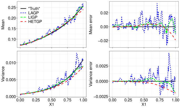
Figure 1: Mean (top) and (bottom) variance estimates (left) and errors (right) for SIR model along the slice $x_{2}=0.2$.

The “local nugget” feature underwhelms when applied globally for many $\mathbf{x}^{\prime}\in\mathcal{X}$ comprising a dense testing set. This can be seen first-hand by trying the examples in the laGP documentation. Figure 1 provides a demo in a stochastic simulation context with a susceptible–infected–recovered (SIR) disease model (Hu and Ludkovski, 2017), implemented as sirEval in hetGP (Binois and Gramacy, 2018, 2021). We used a training set of $\bar{N}=10000$ unique inputs in $[0,1]^{2}$, each paired with a random degree of replication in $\{1,\dots,20\}$, so that the full experiment consisted of $N\approx 100000$ runs. The views in the figure arise from a grid of 200 testing locations along the slice $x_{2}=0.2$. Estimates of the “true” mean and variance (for comparison) are based on smoothed averages of 1000 replicates at each location. Comparators include: LAGP.NN with $n=50$, LIGP.NN with $\bar{n}=100$ ($n\approx 1000$) and $m$=10 inducing points, and HetGP on a random training subset of size $\bar{N}=1000$. Although each comparator incoroporates a different amount of data, which may seem unfair at face value, this was necessary to balance runtime (to within an order of magnitude, in seconds: 0.5, 6.9, and 15.9 respectively) with accuracy. Observe that LAGP’s estimates (blue dashed lines) of the mean and variance are highly discontinuous. The error plots in the right column show how LAGP especially struggles to produce accurate estimates for larger $x_{1}$. Details on our preferred LIGP method (green dashed line), alongside further analysis of this figure, are the subject of Section 3.

The problem with applying LAGP to noisy data is both fundamental and technical. Fundamentally, one needs larger $n$ with noisy data lest the noise dominate the signal, but this severely cuts into efficiency gains. In a technical sense, many stochastic simulation experiments involve replication but the implementation does not adapt its notion of neighborhood accordingly. In the most extreme case, suppose the nearest input site to $\mathbf{x}^{\prime}$ has $n$ replicates. Under that configuration LAGP will degenerate without a diversity of unique training inputs. Less pathologically, a multitude of nearby replicates would effectively result in a narrower $n$-neighborhood even though the number of sufficient statistics is fewer than $n$. This is inefficient both statistically and computationally. Addressing these two issues is the primary contribution of this paper.

2.3 Locally induced GPs

LIGP (Cole et al., 2021) is a recent extension of the LAGP idea that relaxes coupling between neighborhood construction and the local covariance structure. Rather than imposing a local covariance structure on $Y_{n}(\mathbf{x}^{\prime})$ directly via pairwise distances between $\mathbf{X}_{n}(\mathbf{x}^{\prime})\subset\mathbf{X}_{N}$, LIGP uses an intermediary set of $m$ knots, or so-called inducing points or pseudo inputs $\bm{\Psi}_{m}(\mathbf{x}^{\prime})$, whose coordinates are not restricted to $\mathbf{X}_{N}$. This yields speedups by reducing the rank of the covariance structure. When $m\ll n$ there is a double-speedup, first through neighborhood structure ($n\ll N$) and then through low rank local approximation (cubic in $m$ rather than $n$). Conversely, it allows a much larger neighborhood $n$ without cubic-in-$n$ increase in flops.

Let $\mathbf{K}_{m}$ denote a kernel matrix built from inducing points $\bm{\Psi}_{m}(\mathbf{x}^{\prime})$ and $k(\cdot,\cdot)$, e.g., in Eq. (1). We defer a discussion of how one may choose $\bm{\Psi}_{m}(\mathbf{x}^{\prime})$ to Section 3.2. Similarly, write $\mathbf{k}_{nm}$ as cross evaluations of the kernel between $\mathbf{X}_{n}$ and $\bm{\Psi}_{m}$. Adopting the GP approximation with inducing points introduced by Snelson and Ghahramani, (2006) yields

$$\mathbf{\Sigma}_{n}^{(m)}(\mathbf{x}^{\prime})=\tau^{2}\left(\mathbf{k}_{nm}\mathbf{K}_{m}^{-1}\mathbf{k}_{nm}^{\top}+\Delta_{n}^{(m)}+g\mathbb{I}_{n}\right),$$ (2)

as the MVN covariance deployed for inference/prediction at $\mathbf{x}^{\prime}$. Here, $\Delta_{n}^{(m)}=\text{Diag}\{\mathbf{K}_{n}-\mathbf{k}_{nm}\mathbf{K}_{m}^{-1}\mathbf{k}_{nm}^{\top}\}$ is a diagonal correction matrix for the covariance and $g\mathbb{I}_{n}$ expresses the pure noise. Our notation is suppressing some dependence on $\mathbf{x}^{\prime}$ to keep the expressions tidy. Going forward we shall use $\Omega_{n}^{(m)}=\Delta_{n}^{(m)}+g\mathbb{I}_{n}$ to express the sum of diagonal matrices in Eq. (2), electing not to embolden $\Omega_{n}^{(m)}$ like we do for other matrices since it can be stored as an $n$-vector. When $\bm{\Psi}_{m}(\mathbf{x}^{\prime})\equiv\mathbf{X}_{n}(\mathbf{x}^{\prime})$, $\mathbf{\Sigma}_{n}^{(m)}$ reduces to the standard LAGP covariance $\mathbf{\Sigma}_{n}(\mathbf{x}^{\prime})=\tau^{2}(\mathbf{K}_{n}+g\mathbb{I}_{n})$ and offers no computational benefit. The cost savings comes through the decomposition of $\mathbf{\Sigma}_{n}^{(m)}$ (2) through Woodbury matrix identities. Evaluations of $\mathbf{\Sigma}_{n}^{-1(m)}$ and $\log|\mathbf{\Sigma}_{n}^{(m)}|$ may be obtained with $\mathcal{O}(m^{2}n)$ flops rather than $\mathcal{O}(n^{3})$. Likewise, taking $\bm{\Psi}_{m}=\mathbf{X}_{n}=\mathbf{X}_{N}$ with $\mathbf{Y}_{n}=\mathbf{Y}_{N}$ yields a global GP without approximation.

Hyperparameter inference may be achieved by maximizing the logarithm of the MVN likelihood $\mathbf{Y}_{n}\sim\mathcal{N}(\mathbf{0},\mathbf{\Sigma}_{n}^{(m)})$, which may be expressed up to an additive constant as

$$\ell(D_{n}(\mathbf{x}^{\prime}),\bm{\Psi}_{m};\tau^{2},\theta,g) \propto-n\log(\tau^{2})-\log|\mathbf{Q}_{m}^{(n)}|+\log|\mathbf{K}_{m}|-\mathbf{1}_{n}^{\top}\text{log}(\Omega_{n}^{(m)})\mathbf{1}_{n}$$ (3)

$$\qquad-\tau^{-2}\mathbf{Y}_{n}^{\top}\left(\Omega^{-1(m)}_{n}-\Omega_{n}^{-1(m)}\mathbf{k}_{nm}\mathbf{Q}_{m}^{-1(n)}\mathbf{k}_{nm}^{\top}\Omega_{n}^{-1(m)}\right)\mathbf{Y}_{n}.$$

Above, $\mathbf{Q}_{m}^{(n)}=\mathbf{K}_{m}+\mathbf{k}_{nm}^{\top}\Omega_{n}^{-1(m)}\mathbf{k}_{nm}$ and $\mathbf{1}_{n}$ is a vector of $n$ ones. Differentiating Eq. (3) with respect to $\tau^{2}$ yields a closed-form MLE $\hat{\tau}^{2(n,m)}$, see Section 3. A numerical solver like $\tt{optim}$ in $\sf{R}$ can then work with negative concentrated log-likelihood (i.e., plugging $\hat{\tau}^{2(n,m)}$ into Eq. (3)) to estimate $\hat{\theta}^{(n,m)}$ and $\hat{g}^{(n,m)}$. It is important to note that Cole et al., (2021) did not include/estimate a local nugget $g$, which is part of our novel contribution.

For fixed hyperparameters $(\hat{\tau}^{2},\hat{\theta},\hat{g})$, a predictive distribution for $Y(\mathbf{x}^{\prime})$ arises as standard MVN conditioning via an $(n+1)$-dimensional MVN for $(Y(\mathbf{x}^{\prime}),\mathbf{Y}_{n})$. Using $\mathbf{k}_{m}(\mathbf{x}^{\prime})=k_{\theta}(\bm{\Psi}_{m},\mathbf{x}^{\prime})$, the moments of that Gaussian distribution are

$$\mu_{m,n}(\mathbf{x}^{\prime}) =\mathbf{k}_{m}^{\top}(\mathbf{x}^{\prime})\mathbf{Q}_{m}^{-1(n)}\mathbf{k}_{nm}^{\top}\Omega_{n}^{-1(m)}\mathbf{Y}_{m}\hskip 14.22636pt\text{and}$$ (4)

$$\sigma_{m,n}^{2}(\mathbf{x}^{\prime}) =\hat{\tau}^{2}\left(k_{\theta}(\mathbf{x}^{\prime},\mathbf{x}^{\prime})+\hat{g}-\mathbf{k}_{m}^{\top}(\mathbf{x}^{\prime})\left(\mathbf{K}_{m}^{-1}-\mathbf{Q}_{m}^{-1(n)}\right)\mathbf{k}_{m}(\mathbf{x}^{\prime})\right).$$

Both the log-likelihood (3), and predictive equations (4) conditional on those values, reduce to LAGP and ordinary GP counterparts with $\bm{\Psi}_{m}=\mathbf{X}_{n}$ and $\bm{\Psi}_{m}=\mathbf{X}_{n}=\mathbf{X}_{N}$ with $\mathbf{Y}_{n}=\mathbf{Y}_{N}$, respectively. Choosing the locations of inducing points $\bm{\Psi}_{m}$, globally or locally, may also be based on the likelihood (Snelson and Ghahramani, 2006), however this is fraught with issues (Titsias, 2009). Cole et al., (2021) observed that situating $\bm{\Psi}_{m}$ via classical design criteria like integrated variance, or so-called $A$-optimal design, led to superior out-of-sample predictive performance while also avoiding additional cubic calculation. Specifically for local analysis in LIGP, they introduced a weighted form of $\sigma^{2}_{n,m}(\mathbf{x}^{\prime})$, centered around $\mathbf{x}^{\prime}$, and proposed an active learning scheme that minimized weighted integrated mean-square error (wIMSE) for greedy selection of the next element $\bm{\psi}_{m+1}$. Upgraded details are provided in Section 3. Saving on computation by stylizing the feature of the local designs for $\bm{\Psi}_{m}(\mathbf{x}^{\prime})$, Cole et al., developed several template schemes that allow to bypass optimization of wIMSE for each $\mathbf{x}^{\prime}$.

3 Local smoothing under replication

LIGP provides an opportunity to reduce compute time while also increasing neighborhood size, because complexity grows cubically in $m$, not $\bar{n}$ or $n$. This is doubly important when there are replicates among $\mathbf{X}_{N}$. Without inducing points, LAGP neighborhoods of size $n$ could have very few unique inputs $\bar{n}\ll n$. However, LIGP’s Woodbury representation may be extended from inducing points to replicates so that neighborhoods of size $\bar{n}$ may be built, regardless of how much bigger $n$ is, without additional cubic cost.

3.1 Fast GP inference under replication

Given a local neighborhood $D_{n}(\mathbf{x}^{\prime})=(\mathbf{X}_{n}(\mathbf{x}^{\prime}),\mathbf{Y}_{n}(\mathbf{x}^{\prime}))$, let $\bar{\mathbf{x}}_{i}$, $i=1,\dots,\bar{n}$ represent the $\bar{n}\ll n$ unique input locations. Notate each unique $\bar{\mathbf{x}}_{i}$ in $\mathbf{X}_{n}(\mathbf{x}^{\prime})$ as having $a_{i}\geq 1$ replicates, where $\sum_{i=1}^{\bar{n}}a_{i}=n$. Let $y_{i}^{(j)}$ be the response of the $j^{\text{th}}$ replicate of $\bar{\mathbf{x}}_{i}$, $j=1,\dots,a_{i}$. Without loss of generality, assume the $n$-neighborhood inputs are ordered so that $\mathbf{X}_{n}(\mathbf{x}^{\prime})\equiv\mathbf{X}_{n}=(\bar{\mathbf{x}}_{1},\dots,\bar{\mathbf{x}}_{1},\dots,\bar{\mathbf{x}}_{\bar{n}})^{\top}$ with each unique input $\bar{\mathbf{x}}_{i}$ repeated $a_{i}$ times, and suppose $\mathbf{Y}_{n}$ is stacked with responses from the $a_{i}$ replicates in the same order. Based on this construction of $D_{n}$, let $\mathbf{X}_{n}=\mathbf{U}\bar{\mathbf{X}}_{\bar{n}}$, where $\mathbf{U}$ is a $n\times\bar{n}$ block matrix $\mathbf{U}=\text{Diag}(\mathbf{1}_{a_{1}},\dots,\mathbf{1}_{a_{\bar{n}}})$. Defining $\mathbf{U}$ in this way, we have $\mathbf{K}_{n}=\mathbf{U}\mathbf{K}_{\bar{n}}\mathbf{U}^{\top}$ where $\mathbf{K}_{\bar{n}}=(k_{\theta}(\bar{\mathbf{x}}_{i},\bar{\mathbf{x}}_{j}))_{1\leq,i,j\leq\bar{n}}$, while $\mathbf{U}^{\top}\Omega_{n}^{(m)}\mathbf{U}=A_{\bar{n}}\Omega^{(m)}_{\bar{n}}$ where $A_{\bar{n}}=\text{Diag}(a_{i},\dots,a_{\bar{n}})$ and $\Omega_{\bar{n}}^{(m)}=\text{Diag}\{\mathbf{K}_{\bar{n}}-\mathbf{k}_{\bar{n}m}\mathbf{K}_{m}^{-1}\mathbf{k}_{\bar{n}m}^{\top}\}+g\mathbb{I}_{\bar{n}}$.

Using these definitions, we present a new expression for $\mathbf{\Sigma}_{n}^{(m)}$, extending Eq. (2) based on the $\bar{n}$ unique input locations in the local neighborhood:

$$\mathbf{\Sigma}_{n}^{(m,\bar{n})}=\tau^{2}(\mathbf{U}\mathbf{k}_{\bar{n}m}\mathbf{K}_{m}^{-1}\mathbf{k}_{\bar{n}m}^{\top}\mathbf{U}^{\top}+\text{Diag}\{\mathbf{K}_{n}-\mathbf{U}\mathbf{k}_{\bar{n}m}\mathbf{K}_{m}^{-1}\mathbf{k}_{\bar{n}m}^{\top}\mathbf{U}^{\top}\}+g\mathbb{I}_{n}).$$ (5)

While $\mathbf{\Sigma}_{n}^{(m,\bar{n})}$ in (5) is $n\times n$, we do not build it in practice. It is an implicit, intermediate quantity which we notate here as a step toward efficient likelihood and predictive evaluation.

When $m\ll\bar{n}\ll{n}\ll{N}$, decomposing $\mathbf{\Sigma}_{n}^{(m,\bar{n})}$ to obtain $\mathbf{\Sigma}_{n}^{-1(m,\bar{n})}$ and $\log|\mathbf{\Sigma}_{n}^{(m,\bar{n})}|$ is much cheaper than $\mathcal{O}(n^{3})$ under the Woodbury identities. Generically, these are as follows and may be found in most matrix computation resources (e.g., Harville, 1998):

$$(\mathbf{B}+\mathbf{C}\mathbf{D}\mathbf{E})^{-1} =\mathbf{B}^{-1}-\mathbf{B}^{-1}\mathbf{C}(\mathbf{D}^{-1}+\mathbf{E}\mathbf{B}^{-1}\mathbf{C})^{-1}\mathbf{E}\mathbf{B}^{-1}\hskip 14.22636pt\text{and}$$ (6)

$$\log|\mathbf{B}+\mathbf{C}\mathbf{D}\mathbf{E}| =\log|\mathbf{D}^{-1}+\mathbf{E}\mathbf{B}^{-1}\mathbf{C}|+\log|\mathbf{D}|+\log|\mathbf{B}|,$$

where $\mathbf{B}$ and $\mathbf{D}$ are invertible matrices of size $n\times n$ and $m\times m$ respectively, and $\mathbf{C}^{\top}$ and $\mathbf{E}$ are of size $m\times n$. Efficient decomposition in our local approximation context involves combining LIGP’s use of Eq. (6) with inducing points, and Binois et al.,’s (2018a) separate use leveraging replicate structure. Based on (5), let

$$\mathbf{B}=\text{Diag}\{\mathbf{K}_{n}-\mathbf{U}\mathbf{k}_{\bar{n}m}\mathbf{K}_{m}^{-1}\mathbf{k}_{\bar{n}m}^{\top}\mathbf{U}^{\top}\}+g\mathbb{I}_{n},\quad\mathbf{D}=\mathbf{K}_{m}^{-1}\quad\text{and }\mathbf{E}=\mathbf{C}^{\top}=\mathbf{k}_{\bar{n}m}^{\top}\mathbf{U}^{\top}.$$

The result is as follows:

$$\mathbf{\Sigma}_{n}^{-1(m,\bar{n})}= \tau^{-2}\Big{(}\Omega_{n}^{-1(m)}-\mathbf{U}\Omega_{\bar{n}}^{-1(m)}\mathbf{k}_{\bar{n}m}\mathbf{Q}_{m}^{-1(\bar{n})}\mathbf{k}_{\bar{n}m}^{\top}\Omega_{\bar{n}}^{-1(m)}\mathbf{U}^{\top}\Big{)}\hskip 14.22636pt\text{and}$$ (7)

$$\log|\mathbf{\Sigma}_{n}^{(m,\bar{n})}|= \log(\tau^{2})+\log|\mathbf{Q}_{m}^{(\bar{n})}|-\log|\mathbf{K}_{m}|+\sum_{i=1}^{\bar{n}}a_{i}\text{log}\omega_{i}^{(\bar{n},m)},$$

where $\mathbf{Q}_{m}^{(\bar{n})}=\mathbf{K}_{m}+\mathbf{k}_{\bar{n}m}^{\top}\Lambda_{\bar{n}}^{(m)}\mathbf{k}_{\bar{n}m}$, $\Lambda_{\bar{n}}^{(m)}=A_{\bar{n}}\Omega^{-1(m)}_{\bar{n}}$, and $\omega_{i}^{(\bar{n},m)}$ is the $i^{\text{th}}$ diagonal term in $\Omega^{(m)}_{\bar{n}}$. Eq. (7) is key to reducing computational cost from $\mathcal{O}(nm^{2})$ in Eqs. (3–4) to $\mathcal{O}(\bar{n}m^{2})$.

The representations in (7) allow the log-likelihood (3) to be expressed as follows

$$\ell(D_{n},\bm{\Psi}_{m};\tau^{2},\theta,g)\propto -n\log(\tau^{2})-\log|\mathbf{Q}_{m}^{(\bar{n})}|+\log|\mathbf{K}_{m}|-\sum_{i=1}^{\bar{n}}a_{i}\text{log}\omega_{i}^{(\bar{n},m)}$$ (8)

$$-\tau^{-2}\left(\mathbf{Y}_{n}^{\top}\Omega^{-1(m)}_{n}\mathbf{Y}_{n}-\bar{\mathbf{Y}}_{\bar{n}}^{\top}\Lambda_{\bar{n}}^{(m)}\mathbf{k}_{\bar{n}m}\mathbf{Q}_{m}^{-1(\bar{n})}\mathbf{k}_{\bar{n}m}^{\top}\Lambda_{\bar{n}}^{(m)}\bar{\mathbf{Y}}_{\bar{n}}\right),$$

up to an additive constant. Above, $\bar{\mathbf{Y}}_{\bar{n}}$ stores the averaged responses for each unique row $\mathbf{X}_{\bar{n}}$. Notice that when Eq. (7) is applied to the log-likelihood, the $\mathbf{U}$ terms vanish. In fact, we do not need this quantity or $\mathbf{\Sigma}_{n}^{-1(m,\bar{n})}$ except as notational devices. Instead, all matrices in Eq. (8) have dimension in $m$ and/or $\bar{n}$. Although $\mathbf{Y}_{n}^{\top}\Omega^{-1(m)}_{n}\mathbf{Y}_{n}$ must still be calculated, this is a product of vectors, so the entries in $\Omega^{-1(m)}_{n}$ may be stored and accessed through $\Omega_{\bar{n}}^{-1(m)}$ and $A_{\bar{n}}$. Their storage and manipulation are thus linear in $n$.

Differentiating (8) with respect to $\tau^{2}$ and solving, gives the MLE:

$$\hat{\tau}^{2(\bar{n},m)}=n^{-1}\left(\mathbf{Y}_{n}^{\top}\Omega^{-1(m)}_{n}\mathbf{Y}_{n}-\bar{\mathbf{Y}}_{\bar{n}}^{\top}\Lambda_{\bar{n}}^{(m)}\mathbf{k}_{\bar{n}m}\mathbf{Q}_{m}^{-1(\bar{n})}\mathbf{k}_{\bar{n}m}^{\top}\Lambda_{\bar{n}}^{(m)}\bar{\mathbf{Y}}_{\bar{n}}\right).$$ (9)

The equation for $\hat{\tau}^{2(\bar{n},m)}$ in (9) still relies on all replicates through the full $\mathbf{Y}_{n}$ and is equivalent to $\hat{\tau}^{2(n,m)}$ as provided by Cole et al., (2021), Eq. 6. This part of the calculation is linear in $n$. However when replicates are present, evaluation in (9) may be much faster owing to the second term being sized in $\bar{n}$ and $m$. Plugging $\hat{\tau}^{2(\bar{n},m)}$ into Eq. (8) yields the following concentrated negative log likelihood:

$$-\ell\;(D_{n},\bm{\Psi}_{m};\theta,g) \propto n\log\left(\mathbf{Y}_{n}^{\top}\Omega^{-1(m)}_{n}\mathbf{Y}_{n}-\bar{\mathbf{Y}}_{\bar{n}}^{\top}\Lambda_{\bar{n}}^{(m)}\mathbf{k}_{\bar{n}m}\mathbf{Q}_{m}^{-1(\bar{n})}\mathbf{k}_{\bar{n}m}^{\top}\Lambda_{\bar{n}}^{(m)}\bar{\mathbf{Y}}_{\bar{n}}\right)$$ (10)

$$\;\;+\log|\mathbf{Q}_{m}^{(\bar{n})}|-\log|\mathbf{K}_{m}|+\sum_{i=1}^{\bar{n}}a_{i}\text{log}\omega_{i}^{(\bar{n},m)}.$$

The expression above is negated for library-based minimization in search of MLEs $\hat{\theta}^{(\bar{n},m)}$ or $\hat{g}^{(\bar{n},m)}$. Numerical methods such as BFGS (Byrd et al., 1995) work well. Convergence and computing time of such optimizers is aided by closed-form derivatives, which are tedious to derive but are also available in closed form:

$$-\frac{\partial\ell\;(D_{n},\bm{\Psi}_{m},\theta,g)}{\partial\cdot} \propto n\left(\mathbf{Y}_{n}^{\top}\Omega^{-1(m)}_{n}\mathbf{Y}_{n}-\bar{\mathbf{Y}}_{\bar{n}}^{\top}\Lambda_{\bar{n}}^{(m)}\mathbf{k}_{\bar{n}m}\mathbf{Q}_{m}^{-1(\bar{n})}\mathbf{k}_{\bar{n}m}^{\top}\Lambda_{\bar{n}}^{(m)}\bar{\mathbf{Y}}_{\bar{n}}\right)^{-1}$$ (11)

$$\quad\times\frac{\partial\left(\mathbf{Y}_{n}^{\top}\Omega^{-1(m)}_{n}\mathbf{Y}_{n}-\bar{\mathbf{Y}}_{\bar{n}}^{\top}\Lambda_{\bar{n}}^{(m)}\mathbf{k}_{\bar{n}m}\mathbf{Q}_{m}^{-1(\bar{n})}\mathbf{k}_{\bar{n}m}^{\top}\Lambda_{\bar{n}}^{(m)}\bar{\mathbf{Y}}_{\bar{n}}\right)}{\partial\cdot}$$

$$\quad+\text{tr}\left(\mathbf{Q}_{m}^{-1(\bar{n})}\frac{\partial\mathbf{Q}_{m}^{(\bar{n})}}{\partial\cdot}\right)-\text{tr}\left(\mathbf{K}_{m}^{-1}\frac{\partial\mathbf{K}_{m}}{\partial\cdot}\right)+\sum_{i=1}^{\bar{n}}a_{i}\frac{\partial\log\omega_{i}^{(\bar{n},m)}}{\partial\cdot}.$$

Again, observe that none of these log-likelihood-derived quantities (8–11) involve matrices sized bigger than $m\times\bar{n}$.

Conditioning on the estimated hyperparameters leaves us with the following re-expressions of the LIGP predictive equations (4):

$$\mu_{m,\bar{n}}(\mathbf{x}^{\prime}) =\mathbf{k}_{m}^{\top}(\mathbf{x}^{\prime})\mathbf{Q}_{m}^{-1(\bar{n})}\mathbf{k}_{\bar{n}m}^{\top}\Lambda_{\bar{n}}^{(m)}\bar{\mathbf{Y}}_{\bar{n}}\hskip 14.22636pt\text{and}$$ (12)

$$\sigma_{m,\bar{n}}^{2}(\mathbf{x}^{\prime}) =\hat{\tau}^{2(\bar{n},m)}\left(k_{\theta}(\mathbf{x}^{\prime},\mathbf{x}^{\prime})+\hat{g}^{(\bar{n},m)}-\mathbf{k}_{m}^{\top}(\mathbf{x}^{\prime})\left(\!\mathbf{K}_{m}^{-1}-\mathbf{Q}_{m}^{-1(\bar{n})}\right)\mathbf{k}_{m}(\mathbf{x}^{\prime})\right).$$

Although these look superficially similar to (4), the following remarks are noteworthy. Perhaps the biggest difference is that the average of replicates $\bar{\mathbf{Y}}_{\bar{n}}$ is used for the mean. The Woodbury identity ensures that the result is the same as (4), both in mean and variance, if the replicate structure is overlooked. In both cases, many of the details are buried in matrices whose $(\bar{n})$ scripts mask a substantial difference in the subroutines that would be required to build the requisite quantities for (12) as compared to (4).

Kriging with pre-averaged responses $\bar{\mathbf{Y}}_{\bar{n}}$, whether locally or globally, is a common technique for efficiently managing replicates. However, one must take care to (a) adjust the covariance structure appropriately, and (b) utilize all replicates in estimating scale $\hat{\tau}^{2}$. Binois et al., (2018b) show that $\bar{\mathbf{Y}}_{\bar{n}}$ are not sufficient statistics. Using only pre-averaged responses risks leaving substantial uncertainty un-accounted for in prediction. Our Woodbury identities provide a full covariance structure (5), and the adjustments in $n$-quantities for an appropriate scale estimate (9). Alternative approaches, such as Ankenman et al., (2010)’s stochastic kriging (SK), also use unique $\bar{n}$ inputs and pre-averaged outputs. Asymptotically covering (a), it may be shown that SK yields the best linear unbiased predictor (BLUP) when conditioning on estimated hyperparameters. However, the uncertainty in that predictive surface is not fully quantified. For example, SK may only furnish confidence intervals on predictions, not full predictive intervals, because it does not utilize the full set of sufficient statistics (b). Since our Woodbury application links Eq. (12) with (4) identically, a BLUP property holds (locally) for LIGP without asymptotic arguments, and with full predictive UQ.

More specifically, consider the following comparison which upgrades an argument from Binois et al., (2018a) to our local inducing points setting. We show how the MLE of the scale parameter $\tau^{2}$ is not the same (conditioned on $\theta,g$) when calculated on the original set of data versus the unique design locations with averaged responses. Using unique-$\bar{n}$ calculations based on $\bar{\mathbf{Y}}_{\bar{n}}$ only would result in $\bar{\tau}^{2(\bar{n},m)}=\bar{n}^{-1}\bar{\mathbf{Y}}_{\bar{n}}^{\top}\bar{\bm{\Sigma}}_{\bar{n}}^{-1}\bar{\mathbf{Y}}_{\bar{n}}$ where

$$\bar{\bm{\Sigma}}_{\bar{n}}^{(m)}=\mathbf{k}_{\bar{n}m}\mathbf{K}_{m}^{-1}\mathbf{k}_{\bar{n}m}^{\top}+\Delta_{\bar{n}}^{(m)}+gA_{\bar{n}}^{-1},$$ (13)

weights the nugget (noise) based on the number of replicates $a_{i}$ at each unique location $\bar{\mathbf{x}}_{i}$. Our full neighborhood calculation for the local MLE for $\tau^{2}$ with inducing points in Eq. (9) can be rewritten as follows:

$$\hat{\tau}^{2(\bar{n},m)} =N^{-1}\biggl{(}\bar{n}\bar{\tau}^{2(\bar{n},m)}+\mathbf{Y}_{n}^{\top}\Omega^{-1(m)}_{n}\mathbf{Y}_{n}-\bar{\mathbf{Y}}_{\bar{n}}^{\top}\Lambda_{\bar{n}}^{(m)}\bar{\mathbf{Y}}_{\bar{n}}-$$ (14)

$$\qquad\qquad\bar{\mathbf{Y}}_{\bar{n}}^{\top}\bar{\bm{\Sigma}}_{\bar{n}}^{-1(m)}((A_{\bar{n}}^{-1}-\mathbb{I}_{\bar{n}})^{-1}\Delta_{\bar{n}}^{-1(m)}+\bar{\bm{\Sigma}}_{\bar{n}}^{-1(m)})^{-1}\bar{\bm{\Sigma}}_{\bar{n}}^{-1(m)}\bar{\mathbf{Y}}_{\bar{n}}\biggr{)}.$$

See the Appendix for details. Observe that $\bar{\tau}^{2(\bar{n},m)}$ above in Eq. (13) is but a small part of (14). The term following $\bar{\tau}^{2(\bar{n},m)}$ serves as a correction for the variance estimate.

3.2 Local neighborhood geography

To dig a little deeper into the differences between LAGP and LIGP, especially regarding handling replicates and LIGP’s upgraded capability, consider again the SIR example introduced in Section 2.2. Whereas Figure 1 involved a continuum of predictions along a 1d slice, Figure 2 shows relevant quantities involved in one of the locations $\mathbf{x}^{\prime}=(0.47,0.2)$ along that slice, indicated by the green triangle. Recall that the input space is in 2d with $\bar{N}=10000$ unique inputs and replicate degree $a_{i}\in\{1,2,\dots,20\}$ distributed uniformly. With such a high degree of replication, LAGP’s default $n=50$ neighborhood is small, comprising of only $\bar{n}=5$ unique locations. As the green triangle moves along the slice of Figure 1, eventually one of those five will be replaced, resulting in a change in conditioning set of upwards of 1/5 of $\bar{n}$. This provides some of the intuition as to why the LAGP surfaces in Figure 1 are so “jumpy” and often inaccurate.

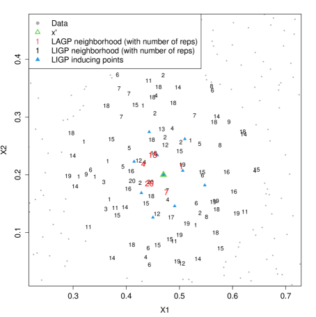
Figure 2: LAGP and LIGP local neighborhoods at $\mathbf{x}^{\prime}=(0.47,0.2)$, with the numbers denoting the number of replicates at each location. Gray dots represent $\mathbf{X}_{N}\setminus\mathbf{X}_{n}$.

LIGP’s implementation of Eqs. (8–12) affords a much larger amount of data in the local model for commensurate computing effort through a template of $m=10$ inducing points. These are indicated as blue triangles in Figure 2. The neighborhood of $\bar{n}=100$ unique design locations are indicated with their number of replicates (black numbers), $n=1091$ in total. In this instance, LIGP conditions upon 20 times more training data than LAGP. This yields more accurate and stable mean and variance estimates, shown visually along a slice in Figure 1 and summarized in a more expansive Monte Carlo (MC) exercise in Section 4.3. Those latter results additionally show that such accurate predictions can be achieved at a computational cost that is substantially lower than LAGP.

The location and spacing of the inducing points $\bm{\Psi}_{m}(\mathbf{x}^{\prime})$ in Figure 2 (blue triangles) come from a local space-filling template scheme based on wIMSE. The idea is that a local inducing point set of a desired size can be built up greedily, using integrated variance under a Gaussian measure centered at $\mathbf{x}^{\prime}$. An expression using $\bar{n}$ unique neighborhood elements (together with all replicates, $n$) given (5) is

$$\text{wIMSE}_{\bar{n}}^{(m+1)}(\bm{\psi}_{m+1},\mathbf{x}^{\prime})=\int_{\breve{\mathbf{x}}\in\mathcal{X}}k_{\theta}(\breve{\mathbf{x}},\mathbf{x}^{\prime})\frac{\sigma_{m+1,\bar{n}}^{2}(\breve{\mathbf{x}})}{\tau^{2}}\;d\breve{\mathbf{x}}$$ (15)

$$\quad=\frac{\sqrt{\theta\pi}}{2}\prod_{k=1}^{d}\Bigg{(}\text{erf}\left\{\frac{\mathbf{x}^{\prime}-a_{k}}{\sqrt{\theta}}\right\}-\text{erf}\left\{\frac{\mathbf{x}^{\prime}-b_{k}}{\sqrt{\theta}}\right\}\Bigg{)}-\text{tr}\Big{\{}\Big{(}\mathbf{K}^{-1}_{m+1}-\mathbf{Q}^{-1(\bar{n})}_{m+1}\Big{)}\mathbf{W}^{\prime}_{m+1}\Big{\}},$$

where erf is the Gaussian error function, $a_{k},b_{k}$ are bounds for a hyperrectangle study region $\mathcal{X}=[a_{k},b_{k}]_{k=1}^{d}$, and $\mathbf{W}^{\prime}_{m+1}=\prod_{k=1}^{d}\mathbf{W}^{\prime}_{m+1,k}$. Again, the resemblance to a similar expression from Cole et al., (2021) masks a substantial enhancement in its component parts due to a double-Woodbury application, as notated by $\bar{n}$ scripts. The $(i,j)^{\text{th}}$ entry of $\mathbf{W}^{\prime}_{m+1,k}$ is $w_{m+1,k}(\bm{\psi}_{i},\bm{\psi}_{j})$ defined in Eq. (11) in Cole et al., (2021). A closed-form gradient with respect to $\bm{\psi}_{m+1}$ may also be derived. This is similar in form to Cole et al.,, so we do not duplicate it here. Given $\mathbf{Q}^{-1(\bar{n})}_{m+1}\equiv\mathbf{Q}^{-1(n)}_{m+1}$, the calculation in (15) and derivative are equivalent to Eqs. (10–12) in that paper. Consequently, a wIMSE optimized design of inducing points is not affected by the local distribution of replicates. Under replication $\mathbf{Q}^{-1(\bar{n})}_{m+1}$ can, of course, be calculated much faster than $\mathbf{Q}^{-1(n)}_{m+1}$, so the optimization is speedier.

Regularity in local inducing point design also means that simple space-filling designs can serve as thrifty substitutes to the wIMSE design with similar predictive accuracy. The qNorm method (Cole et al., 2021) transforms a space-filling design with the inverse-CDF of a Normal distribution to mimic an wIMSE inducing point design. This is what was used for Figures 1–2. Once a set of inducing points $\bm{\Psi}_{m}(\mathbf{x}^{\prime})$ is calculated for one $\mathbf{x}^{\prime}$, Cole et al., (2021) show that it can serve as a template for predictions at other members of a testing set $\mathcal{X}$ through displacement and warping, so long as the characteristics of the original design $\mathbf{X}_{N}$ are uniform. Templates based on wIMSE tend to fill the neighborhood in a more uniform manner than via qNorm, providing a higher density of inducing points near the predictive location. This often leads to more accurate prediction. Yet the reduced time required to build qNorm templates is also beneficial. We contrast both options in our empirical work in Section 4.

4 Implementation and benchmarking

Now we provide practical details and report on experimental results showcasing LIGP’s potential for superior accuracy and UQ at lower computational costs against LAGP and HetGP. Our examples include data from a toy function and real stochastic simulators. All analysis was performed on an eight-core hyperthreaded Intel i9-9900K CPU at 3.60 GHz. Every effort was made to take advantage of that distributed resource to minimize compute times.

4.1 Implementation details

Open source implementation of LIGP can be found in the liGP package on CRAN (Cole, 2021). R code (R Core Team, 2020) supporting all examples reported here and throughout the paper, may be found on our Git repository.

https://bitbucket.org/gramacylab/ligp/src/master/noise

Our main competitors are laGP (Gramacy, 2016) and hetGP (Binois and Gramacy, 2018). While laGP is coded in C with OpenMP for symmetric multiprocessing (SMC) parallelization (R serving only as wrapper), and hetGP leverages substantial RCpp (Eddelbuettel, 2013), our LIGP implementation coded purely in R using foreach for SMC distribution. With laGP we use the default neighborhood size of $n=50$ built by NN and Active Learning Cohn (ALC; Cohn, 1994), representing distance- and variance-based (similar to wIMSE) approaches, respectively. For hetGP, we reduce the training data to a random subset of $\bar{N}=1000$ unique inputs (retaining all replicates) to keep decompositions tractable. Despite compiled C/C++ libraries and thrifty (local/global) data subset choices, our (more accurate and larger-neighborhood) LIGP models are competitive, time-wise, and sometimes notably faster.

Our LIGP implementation uses an isotropic Gaussian kernel with scalar lengthscale $\theta$. To improve numerical conditioning of matrices $\mathbf{K}_{m}$ and $\mathbf{Q}_{m}^{(n)}$ for stable inversion, we augment their diagonals with $\epsilon_{K}=10^{-8}$ and $\epsilon_{Q}=10^{-5}$ jitter (Neal, 1998), respectively. Our implementation in liGP automatically increases these values for a particular local model if needed. LAGP and HetGP results also utilize an isotropic Gaussian kernel. Using separable local formulations do not significantly improve predictive performance, especially after globally prescaling the inputs (Sun et al., 2019). Pre-scaling or warping of inputs (Wycoff et al., 2021) has become a popular means of boosting predictive performance of sparse GPs (e.g., Katzfuss et al., 2020). In our exercises, we divide by square-rooted separable global lengthscales obtained from a GP fit to random $\bar{N}=1000$ data subsets with averaged responses $\bar{\mathbf{Y}}_{\bar{N}}$. See Gramacy, (2020), Section 9.3.4, for details. The time required for this, which is negligible relative to other timings, is not included in our summaries.

For inducing point designs $\bm{\Psi}_{m}(\mathbf{x}^{\prime})$, we use wIMSE templates based on Eq. (15) built at the center of the design space $\check{\mathbf{x}}$, determined as the median of $\mathbf{X}_{N}$ in each dimension. For initial local lengthscale $\theta^{(0)}$, we adopt a strategy from laGP via the 10% quantile of squared pairwise distances between members of $\mathbf{X}_{n}$. When selecting each $\bm{\psi}_{m+1}$ to augment $\bm{\Psi}_{m}$, optimizing wIMSE is conducted via a 20-point multi-start derivative-based L-BFGS-B (Byrd et al., 1995) scheme (using optim in R to a tolerance of 0.01) peppered within the bounding box surrounding the neighborhood $\mathbf{X}_{n}$. In addition to the wIMSE design for the inducing point template, we consider so-called “qNorm” templates derived from space-filling designs. These originate from $m-1$ point Latin hypercube samples (LHS; Mckay et al., 1979) on the hyperrectangle enclosing $\mathbf{X}_{n}(\check{\mathbf{x}})$, augmented with $\check{\mathbf{x}}$ as the $m^{\mathrm{th}}$ point. These LHSs are warped with the inverse Gaussian CDF to closely mimic the wIMSE design.

Individual local neighborhoods and predictions are made for a set of $N^{\prime}$ testing locations $\mathbf{x}^{\prime}\in\mathcal{X}$ given training data $\{\mathbf{X}_{N},\mathbf{Y}_{N}\}$, neighborhood size $\bar{n}$, and number of inducing points $m$. We use $\bar{n}=100$ for each experiment, with $m=10$ and $30$ for the 2d and 4d problems, respectively. Each location $\mathbf{x}^{\prime}_{i}$, for $i=1,\dots,N^{\prime}$ proceeds in parallel via 16 foreach threads. To estimate scale and lengthscale, we used Eqs. (9–11) via optim through the local neighborhoods of $\mathbf{x}^{\prime}$. To aid in discerning signal from noise during hyperparameter optimization, we incorporate default priors for $\theta$ and $g$, from laGP, described in Appendix A of Gramacy, (2016). Predictions follow Eq. (12).

4.2 Benchmark non-stationary data

The toy 2d function known as Herbie’s tooth (Lee et al., 2011) is attractive as a benchmark problem due to its non-stationary mean surface with multiple local minima. The mean function is defined by $f(x_{1},x_{2})=-w(x_{1})w(x_{2})$, $x_{1},x_{2}\in[-2,2]$, where

$$w(x)=\text{exp}\left\{-(x-1)^{2}\right\}+\text{exp}\left\{-0.8(x+1)^{2}\right\}-0.05\sin\left(8(x+0.1)\right).$$

For this experiment we introduce constant noise $\epsilon\sim N(0,0.02^{2})$, creating a response $y(x_{1},x_{2})=f(x_{1},x_{2})+\epsilon$. Each of the 30 MC repetitions is comprised of a fresh training set of $\bar{N}=10000$ LHS locations, each with $a_{i}\stackrel{{\scriptstyle\mathrm{iid}}}{{\sim}}\mathrm{Unif}\{1,2,\dots,20\}$ for $i=1,\dots,\bar{N}$. Although our later experiments use a more common, fixed-degree setup for replicates, we choose random $a_{i}$ here to underscore that LIGP does not require a minimum amount of replication. A separate LHS of $N^{\prime}=10000$ out-of-sample testing locations is created for each MC run. Our LAGP fits include $n=100$ via NN for a slightly fairer comparison to LIGP, in addition to the other LAGP options described earlier.

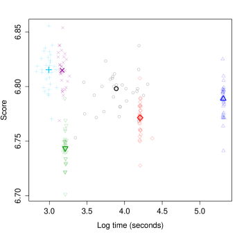
Figure 3: RMSE (left) and score (right) vs. log compute time over 30 MC repetitions for Herbie’s tooth experiment. Median statistics are denoted with bold markers.

Figure 3 shows out-of-sample accuracy statistics versus the logarithm of compute time across the MC repetitions. A particular method’s median statistic, taken marginally across both axes, is represented with a bold symbol. The left panel shows the root mean-squared prediction error (RMSE; lower is better) against the (de-noised) truth along the vertical axis. In the right panel, the vertical axis shows proper scores (higher is better), combining mean and variance (UQ) accuracy (Gneiting and Raftery, 2007, Eq. (27)) against the (noisy) test data. Concretely, RMSE (lower is better) and score (higher) follow:

$$\text{RMSE}=\sqrt{\sum_{i=1}^{N^{\prime}}(\hat{\mu}(\mathbf{x}_{i})-y(\mathbf{x}_{i}))^{2}}\hskip 11.38092pt\text{and}\hskip 11.38092pt\text{Score}=-\sum_{i=1}^{N^{\prime}}\frac{\left(\hat{\mu}(\mathbf{x}_{i})-y(\mathbf{x}_{i})\right)^{2}}{\hat{\sigma}^{2}(\mathbf{x}_{i})}-\sum_{i=1}^{N^{\prime}}\hat{\sigma}^{2}(\mathbf{x}_{i}).$$

LIGP methods yield the fastest predictions with the lowest RMSEs and highest scores. Our LIGP.qNorm (blue $+$’s) has the quickest compute time. LAGP.NN with $n=50$ (green inverted triangles) is the fastest among the LAGP models, but is least accurate. HetGP (black circles) is fit with substantial sub-setting, which explains its high-variance metric on both time and accuracy. Notice that LAGP.ALC (red diamonds) and LAGP.NN ($n=100$; navy triangles) perform similarly for RMSE, but the latter has a higher score. This supports our claim that a wider net of local training data is needed to better estimate noise.

4.3 Susceptible-infected-recovered (SIR) epidemic model

We return to the SIR model (Hu and Ludkovski, 2017) first mentioned in Section 2.2. SIR models are commonly used for cost-benefit analysis of public health measures to combat the spread of communicable diseases such as influenza or Ebola. We look at a simple model with two inputs: $x_{1}$ the initial number susceptible individuals; and $x_{2}$ the number of infected individuals. In hetGP (Binois and Gramacy, 2018), the function sirEval accepts these two inputs on the unit scale. The response of the model is the expected aggregate number of infected-days across Markov chain trajectories until the epidemic ends. The signal-to-noise ratio varies drastically throughout $\mathcal{X}$, making this model an ideal test problem for LIGP.

In this experiment we keep the same $\bar{N}=10000$ training set size as Section 4.2, but now use a fixed degree of 10 replicates at each location, a more common default design setup in the absence of external information about regions of high/low variability. We also keep a large $N^{\prime}=10000$ testing set, which helps manage MC error in our out-of-sample metrics in this heteroskedastic setting. The experiment’s results are displayed in Figure 4. The left panel’s vertical axis shows the RMSE values between each method’s mean predictions and the noisy testing observations. Variability across repetitions in the data generating mechanism looms large compared to the differences in RMSE values among the methods. Although RMSE/scores may look similar marginally, within each MC repetition there is a clearer ordering. To expose that, the left section of Figure 4’s table ranks the methods based on their RMSE (lowest/best first). The reported $p$-values are for one-sided paired Wilcoxon tests between a method’s RMSE and the RMSE from the next best fit. Observe, for example, that LIGP.qNorm (blue $+$’s) produces a significantly lower distribution of RMSEs compared to the other models, with LIGP.wIMSE (purple $\times$’s) and HetGP (black circles) not far behind.

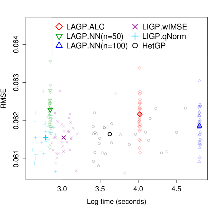
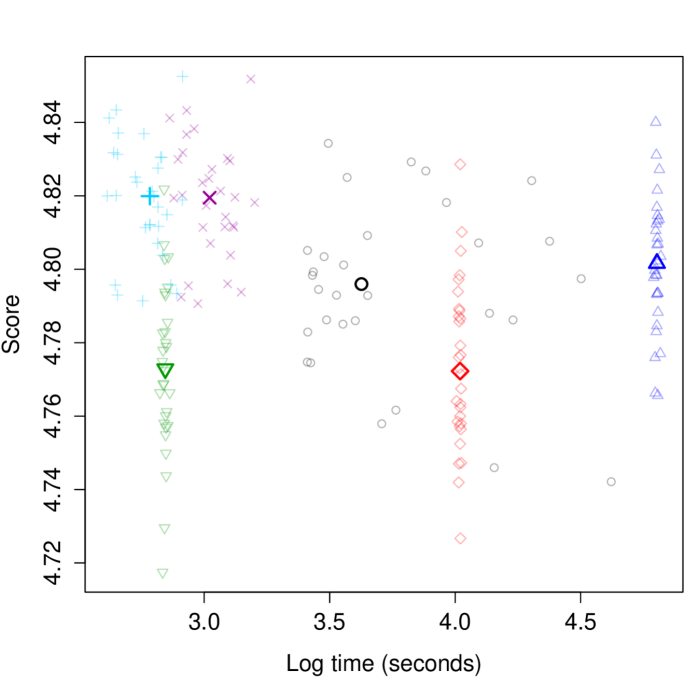
Model	RMSE	$p$-value	Model	Score	$p$-value	Time
LIGP.qNorm	0.06156	0.0041	LIGP.qNorm	4.82	0.0031	16.2
LIGP.wIMSE	0.06156	0.6348	LIGP.wIMSE	4.819	$<10^{-9}$	20.5
HetGP	0.06165	$<10^{-8}$	LAGP.NN ($n$=100)	4.802	0.0288	122
LAGP.NN ($n$=100)	0.06186	$<10^{-9}$	HetGP	4.796	$<10^{-5}$	37.6
LAGP.ALC ($n$=50)	0.06217	$<10^{-7}$	LAGP.NN ($n$=50)	4.773	0.7860	17.2
LAGP.NN ($n$=50)	0.06229		LAGP.ALC ($n$=50)	4.772		55.7

Figure 4: Top: RMSE (left) and score (right) vs. log compute time over 30 MC repetitions for the SIR experiment. Median statistics are denoted with bold markers. Bottom: Median RMSEs (left) and scores (right) in ascending rank. The $p$-values are for one-sided paired Wilcoxon tests between the model and the model directly below. Median compute time (in seconds) for each model is listed in the last column.

Score (right panel) offers clearer distinctions between the methods, with LIGP besting LAGP and HetGP via paired Wilcoxon test. Using score as a metric highlights the differences in accuracy for the model estimates. By weighting the squared error by the predictive variance, not all errors of the same magnitude are considered equal (unlike in RMSE), which is crucial when modeling a heteroskedastic process. LIGP.qNorm and LIGP.wIMSE are statistically distinguishable from each other ($p$-value $<0.01$) and better than LAGP.NN with $n=100$ ($p$-value $<10^{-9}$), the next in the list. There is more variation in the computation times of the LIGP models compared to LAGP, which is likely due to LIGP’s tendency to need more function evaluations for hyperparameter optimization. LIGP provides significant time savings despite an R implementation.

4.4 Ocean oxygen concentration model

Here we consider a stochastic simulator modeling oxygen concentration deep in the ocean (McKeague et al., 2005). This highly heteroskedastic simulator uses MC to approximate the solution of an advection-diffusion equation from computational fluid dynamics. There are four inputs: latitude and longitude coordinates, and two diffusion coefficients. The code required to run the simulation can be found in our repository. Inputs are scaled to the unit cube $[0,1]^{4}$; the output is the ocean oxygen concentration.

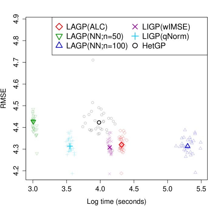
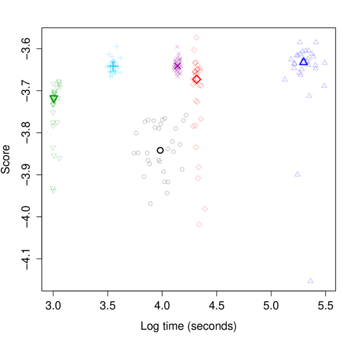
Model	RMSE	$p$-value	Model	Score	$p$-value	Time
LIGP.wIMSE	4.3078	0.0759	LAGP.NN ($n$=100)	-3.633	0.0502	199.8
LAGP.NN ($n$=100)	4.3135	0.0202	LIGP.wIMSE	-3.641	0.0013	62.9
LIGP.qNorm	4.3137	0.0005	LIGP.qNorm	-3.642	$<10^{-4}$	34.8
LAGP.ALC ($n$=50)	4.3202	$<10^{-9}$	LAGP.ALC ($n$=50)	-3.673	0.0060	74.9
LAGP.NN ($n$=50)	4.4271	0.9725	LAGP.NN ($n$=50)	-3.717	$<10^{-5}$	20.2
HetGP	4.4230		HetGP	-3.842		53.6

Figure 5: Top: RMSE (left) and score (right) vs. log compute time over 30 MC repetitions for Ocean Oxygen experiment. See Figure 4 caption.

We keep the same training/testing set sizes from the SIR experiment: $\bar{N}=10000$ with 10 replicates each and $N^{\prime}=10000$. Figure 5 shows out-of-sample metrics similarly mirroring that experiment. At first glance, HetGP (black circles) is clearly worse (higher RMSEs, lower scores) than LIGP/LAGP. In 4d, using a subset of only 1000 unique locations does not provide enough information to model this surface. The variation in compute time for HetGP, due to challenges in modeling the latent noise, support this claim.

Focusing on LIGP and LAGP results, we find LIGP again among the best in RMSE, score, and computation time. LAGP.NN with the larger neighborhood of $n=100$ (navy triangle) does well at modeling the mean and noise surfaces (its RMSE and score medians are comparable to the LIGP models), but takes nearly 6 times longer than LIGP.qNorm. HetGP (black circles) and LAGP.ALC (red diamonds) model the mean surface well, producing slightly worse RMSEs, but struggle with UQ as measured by proper score.

5 Bermudan Option Pricing

An application of high-throughput stochastic simulation arises in computational methods for optimal stopping, which are particularly motivated by quantitative finance contexts. Several types of financial contracts – the so-called American-type claims – offer their buyer the option to exercise, i.e., collect, her contract payoff at any time until its maturity. Pricing and risk managing such a contract requires analysis of the respective optimal exercise strategy, such deciding when to exercise the option.

Monte-Carlo-driven valuation of American-type claims consists of applying the dynamic programming formulation to divide the global dynamic control problem into local single-step optimization sub-problems. The latter revolve around partitioning the input space (interpreted as the underlying prices at the current time-step) into the exercise and stopping regions, to be learned by constructing a certain statistical surrogate. More precisely, one wishes to compare the $q$-value, namely the expected future payoff conditional on not exercising now, with the immediate payoff. While the latter is a known function, the $q$-value is specified abstractly as a recursive conditional expectation and must be learned.

In the literature (Binois et al., 2018a; Ludkovski, 2018, 2020), it has been demonstrated that GP surrogates are well suited for this emulation task, due to their flexibility, few tuning parameters, and synergy with sequential design heuristics. Nevertheless, their cubic scaling in design size $N$ is a serious limitation. The nature of the financial context implies an input space is 2-5 dimensional (1d problems are also common but are computationally straightforward) and a very low signal-to-noise ratio. Consequently, Monte Carlo methods for accurate estimation of the $q$-value call for $N\gg 10^{4}$ simulations. Ludkovski, (2018) demonstrated that replication is pivotal to addressing this scaling challenge; Lyu and Ludkovski, (2022) explored adaptive replication. LIGP offers an additional boost by leveraging replication and local approximation, simultaneously addressing speed, accuracy and localization.

Relative to existing surrogates LIGP brings several improvements. First, it overcomes limitations on the number of training simulations $N$. In previous experiments working with matrices of size $\gg 2000$ was prohibitively slow. This limited traditional GPs to data with dimension $d\leq 3$ or excessive replication. Second, LIGP organically handles replicated designs that are needed to separate signal from noise, which is heteroskedastic and non-Gaussian in this application. Third, the localization intrinsic in LIGP is beneficial to capture non-stationarity. Typically the $q$-value is flat at the edges and has a strong curvature in the middle of the input space. Finally, the control paradigm implies that the surrogate is intrinsically prediction-driven – the main use-case being to generate exercise rules along a set of price scenarios. Thus, the surrogate is to be evaluated at a large number of predictive locations and LIGP offers trivial parallelization that vastly reduces compute time relative to plain GP variants.

5.1 Illustrating the Exercise Strategy

We have added LIGP regressors as a new choice to the mlOSP library (Ludkovski, 2020) for R, which contains a suite of test cases that focus on valuation of American-type options on multiple assets. This allows benchmarking the LIGP module against alternatives, including plain GP and hetGP solvers that are already part of mlOSP.

To fix ideas, we consider the $d$-dimensional Bermudan Max-Call with payoff function

$$h_{\mathrm{MaxCall}}(k,\mathbf{x})=e^{-rk\Delta t}(\max_{i\leq d}x_{i}-{\cal K})_{+}.$$

The parameter ${\cal K}$ is known as the strike, $r$ is the continuously compounded interest rate and $\Delta t$ is the exercise frequency measured in calendar time (e.g. daily, $\Delta t=1/365$). The input space $\mathbf{x}\in\mathbb{R}^{d}_{+}$ represents prices $x_{1},\ldots,x_{d}$ of $d$ stocks. Thus, the buyer of the Max-Call is able to collect $h_{\mathrm{MaxCall}}(k,\mathbf{X}(k\Delta t))$ dollars, the difference between the largest stock price and the strike, at any one of the $K$ exercise opportunities, $k=1,\ldots,K$. The choice of when to do so leads to $K$ decisions regarding whether to exercise the option at time step $k$ (assuming it was not exercised yet) or not. Thus, we need $K-1$ surrogates for the $q$-value $q(k,\mathbf{x})$, $k=0,\ldots,K-1$.

The underlying stochastic simulator is based on generating trajectories of the asset prices. We stick to independent log-normal (Geometric Brownian motion) dynamics for the price of the $i^{\mathrm{th}}$ asset,

$$dX_{i}(t)=(r-\delta_{i})X_{i}(t)dt+\sigma_{i}X_{i}(t)dW_{i}(t),\qquad i=1,\ldots,d,$$ (16)

where $W_{i}(t)$ are independent standard Brownian motions, $\sigma_{i}$ is the volatility, and $\delta_{i}$ the continuous dividend yield of the $i$-th asset. This implies that given $X_{i}(s)$ for any $t>s$, $X_{i}(t)$ has a log-normal distribution. Denote by $\mathbf{X}_{k:K}=\mathbf{X}_{k\Delta t},\ldots,\mathbf{X}_{K\Delta t}$ a realized trajectory of the $d$ asset prices on the interval $[k\Delta t,K\Delta t]$.

The stochastic simulator yields empirical samples of $H_{k}(\mathbf{X}_{k},\mathbf{X}_{k+1},\ldots,\mathbf{X}_{K})$ where the aggregate function $H_{k}$, representing the pathwise payoff, is a selector

$$H_{k}(\mathbf{x}_{k},\ldots,\mathbf{x}_{K})=\left\{\sum_{s=k+1}^{K}h(s,\mathbf{x}_{s})1_{A_{s}}\right\}-h(k,\mathbf{x}_{k}),$$

and $A_{k}$ records the first pathwise exercise time along the given trajectory. The objective of learning the $q$-value at step $k$ is equivalent to regressing $H_{k}$ against $\mathbf{x}_{k}$ (exploiting the Markov property of the state dynamics) to obtain the so-called timing value $\hat{T}_{k}(\mathbf{x}_{k})$ and identify regions where the conditional mean is positive/negative. Note that this task must be done for each time step $k=K-1,\ldots,1$, and by construction the outputs at step $k$ depend on the $\hat{T}_{k+1:K-1}$’s fitted previously. This iterative estimation leads to non-trivial error back-propagation along the financial time dimension in $k$.

Returning to the LIGP implementation, we have a sequence of surrogates that must be constructed. For each surrogate, we are given a data set of size $N$ with $\bar{N}$ unique inputs in $\mathbb{R}^{d}_{+}$ and a constant number of replicates $a$, $N=\bar{N}\cdot a$. For the experimental design we take an LHS on a user-specified sub-domain. After fitting the surrogate for $\hat{T}_{k}$, we need to predict on $N^{\prime}=N$ unique outputs, which lie in the training sub-domain but are otherwise distinct from the training inputs.

To illustrate how that looks, Figure 6 compares global GP and LIGP fits for the timing value of the 2d Bermudan Max-Call option. The model parameters are ${\cal K}=100$, $r=0.05$, $\delta_{1}=\delta_{2}=0.1$, $\sigma_{1}=\sigma_{2}=0.2$, $T=3$ and $\Delta t=1/3$ so that there are $K=9$ time periods. We display the fitted surrogates at one intermediate time step, $k=6$. In this problem, the option is out-of-the-money when both $x_{1}$ and $x_{2}$ are below the strike ${\cal K}=100$, hence the exercise strategy is to continue in that region and the latter (the white square in the bottom-left of each panel) is excluded from the surrogate prediction. For both problems, we have a randomized training set of $\bar{N}\approx 650$ inputs, with $a=25$ replicates each, created by a LHS design. The LIGP surrogate uses $m=10,n=50$, with estimated nugget and fixed lengthscale $\theta=1$.

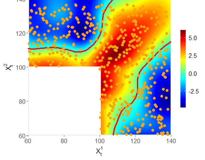
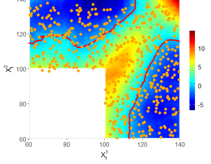
Figure 6: Fitted timing value and the corresponding exercise boundary (solid red curves) for the global GP (left) and LIGP (right) for the 2-d Max-Call problem at time step $k=6$. The colors indicate the fitted $\hat{T}_{k}(x_{1},x_{2})$ and the points the training inputs $\mathbf{x}=(x_{1},x_{2})$. The bottom left corner is excluded from the input space since it has zero payoff.

The estimated strategy is to continue when the timing value $\hat{T}_{k}$ (color coded in both panels) is positive and to stop when it is negative, with the zero-contour (in red) demarcating the boundary of the stopping region. The stopping region consists of two disconnected components, in the bottom-right and upper-left; due to the symmetric choice of parameters, those regions (and the entire response) are symmetric along the $x_{1}=x_{2}$ diagonal. Thus, the response surface features a diagonal ridge with a global maximum around $(100,100)$ and two basins on either side. The height of the ridge and the depth of the basins change in $k$. The respective simulation variance is low in regions where $T_{k}(\mathbf{x})\simeq 0$ and is high in regions where $|T_{k}(\mathbf{x})|$ is large.

We emphasize that Figure 6 is purely diagnostic; actual performance of the surrogate is based on the resulting estimated option price. The latter is obtained by generating a test set of $N^{\prime}$ scenarios and using the collection of $K$ surrogates $\hat{T}_{k}$, $k=0,\ldots,K-1$ to evaluate the resulting exercise times and ultimately the average payoff. Fixing a test set, the surrogate that yields a higher expected payoff is deemed better. Traditionally, a test set is obtained by fixing an initial $\mathbf{X}(0)$ and sampling $N^{\prime}$ i.i.d. paths of $\mathbf{X}_{0:K}$. For example, taking $\mathbf{X}(0)=(90,90)$ and using the surrogates displayed in Figure 6 we obtain an estimated Max-Call option value of 8.02 via LIGP and 8.00 via the global GP. Note that this financial assessment of surrogate accuracy is not based on standard IMSE-like metrics, but is driven by the accuracy of correctly learning the exercise strategy, namely the zero-contour of $H_{k}$. Hence, the goal is to correctly specify the sign of $T_{k}(\mathbf{x})$ which determines whether the option is exercised in the given state or not. Consequently, errors in the magnitude of $\hat{T}_{k}$ are tolerated, while errors in the sign of $\hat{T}_{k}$ will lead to degraded performance.

5.2 Results for Bermudan Option Pricing

The 2d example was primarily for illustrative purposes; for a more challenging case we take a 5d asymmetric Max-Call. We keep $T=3,\Delta t=1/3,{\cal K}=100,r=0.05$ but adjust the parameters of the log-normal asset dynamics (16) to be $\delta_{1}=\ldots=\delta_{5}=0.1$ and $\sigma_{i}=0.08\cdot i$ to have different volatilities. The setting therefore is no longer symmetric and, due to larger variance, the third-through-fifth coordinates are progressively more important. The initial starting point is taken to be $\mathbf{X}(0)=(70,70,70,70,70)$.

We benchmark the results on a fixed test set of $N^{\prime}=25000$ paths of $\mathbf{X}(t)$, comparing the resulting option price estimates. Our comparators include a global GP model homGP and a hetGP surrogate. Note that the above are not pre-scaled and take inputs as-is. We train the surrogates with an experimental design sampled from the log-normal density of $\mathbf{X}(t)$, with $\bar{N}=2000$ unique inputs and $a=10$ replicates each. In this case study we found that a relatively small number of inducing points $m=30$ works well along with a neighborhood size of $n=50$. We also left out various embellishments that can further fine-tune each surrogate, aiming for a level playing field.

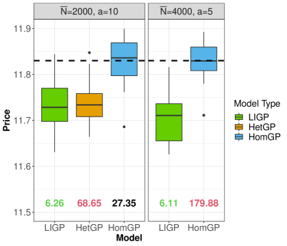
Figure 7: Results for the 5d Asymmetric Bermudan Max-Call. Distributions of price over 30 MC repetitions. Average compute time (mins) is below each box plot. All LIGP models (green) use the qNorm template. The default setting is $\bar{N}=2000,a=10,n=50$.

Figure 7 presents the results, with the average compute times (in minutes) below each box plot. The reported compute time is for the entire option pricing problem, i.e., across $K=9$ surrogates. The reference option price is $11.83$ (black dashed line). With a design of $\bar{N}=2000$, all three approaches yield similar results that are close to optimal, but the compute times vary substantially. LIGP is more than four times faster than homGP and an order of magnitude faster than hetGP. In the problem context, methods that take more than a handful of minutes are impractical, and these major speedup gains greatly outweigh the small accuracy loss with LIGP. Not shown in Figure 7 are the results from laGP. Using LAGP.ALC with $n=50$ is prohibitively slow in this example (over an hour, like hetGP), while using LAGP.NN yields very poor prices (below 11.5). Thus, laGP fails either in terms of speed or in terms of accuracy and is not a viable alternative.

Exploration of the input space tends to be the main driver of accuracy, so we consider upgrading to $\bar{N}=4000$ and $a=5$ replicates. This keeps the same budget for total number of simulations but is more exploratory. The new choice has minimal impact on the compute time of LIGP that is driven by $\bar{N}\times a$ and is to zeroth-order independent of $\bar{N}$. Indeed, the average compute times between $4000\times 5$ (6.11 mins) and $2000\times 10$ (6.26) are within 3% of each other. On the other hand, $\bar{N}\gg 10^{3}$ is too large for a global GP: homGP takes nearly three hours with $\bar{N}=4000$ and hetGP is not considered as it takes even longer.

Running times that exceed an hour (shown in red in Figure 7) are prohibitive. A take-away here is that with a global approach one is restricted in the choice of $\bar{N}$, while LIGP has additional flexibility to survey the exploration-exploitation tradeoff. In this particular setting, having more unique inputs does not yield substantial performance improvement, but in related contexts it is a crucial factor for developing an accurate exercise strategy.

6 Discussion

Modern computing resources and advances in MC and agent-based modeling strategies have combined of late to produce large simulation campaigns for complex phenomena. The ability to adequately model such large data sets is limited, especially when the simulator is heteroskedastic. Methods for modeling large data sets exist, such as sparse matrix approximation and divide-and-conquer, but are easily fooled into interpreting noise as signal and provide inadequate UQ in the presence of input-dependent noise.

Local approximations (LAGP) on local subsets of data (neighborhoods) perform well on predictive accuracy for deterministic data, because small local subsets yield a substantial computational advantage over competing methods. Scaling up to larger neighborhoods in the face of common replication-based design strategies for separating signal from noise is problematic in that context; larger neighborhoods wipe out that computational advantage. LIGP frees up resources through inducing points, and thus allow for increases in neighborhood size without severe computational bottlenecks, but is developed solely for deterministic data. HetGP was designed for heterogeneous noisy simulations, and replicated responses in the experimental design, and consequently makes thrifty use of sufficient statistics and provides excellent UQ. But it is not a local approximation, and so it does not scale well to the largest simulation campaigns.

Here we provide upgrades to the LIGP framework, essentially by combining these three modern methods. We first redefine LIGP neighborhoods based on the number of unique design locations. Applying the common Woodbury identities allows us to take advantage of replication. This provides calculations on the order of the number of inducing points and unique locations. Consequently LIGP may entertain much larger neighborhoods compared to LAGP and the original version of LIGP. With these larger neighborhoods, we present evidence that LIGP is able to better, and more quickly, separate signal from noise.

The promising results in this paper provide direction for further areas of study. While current work relies on NN to build local neighborhoods, variance-based alternatives (e.g., alcray in laGP, Gramacy and Haaland, (2016)) may enhance modeling the mean surface. Extending the kernel support to other families such as Matérn (Stein, 2012) may also prove useful. Our empirical work relied on default choices of $(m,n)$ without much exploration. A better understanding of these hyperparameters (possibly through Bayesian optimization of out-of-sample RMSE or score) could yield better defaults for simple, immediate implementation.

It is worth reinforcing every aspect of our local GP fits is unique to each local neighborhood, providing a discontinuous noise (and mean) surface. This is in contrast to global methods (e.g., HomGP, HetGP). We find that the computational and other model fidelity advantages of such a local approach outweigh the superficial disadvantages of a sometimes “choppy” predictive surface. That said, local-global approach where noise information is shared across neighborhoods (Edwards and Gramacy, 2021) could help smooth the noise across the input space.

Appendix

Here we provide more details for re-expressing $\hat{\tau}^{2(\bar{n},m)}$ in Eq. (9) as Eq. (14). Based on Binois et al., (2018a), we can re-write $\hat{\tau}^{2(\bar{n},m)}$ as

$$\hat{\tau}^{2(\bar{n},m)}=N^{-1}\left(\mathbf{Y}_{n}^{\top}\Omega^{-1(m)}_{n}\mathbf{Y}_{n}-\bar{\mathbf{Y}}_{\bar{n}}^{\top}\Lambda^{(m)}_{\bar{n}}\bar{\mathbf{Y}}_{\bar{n}}+\bar{n}\grave{\tau}^{2(\bar{n},m)}\right)$$

where $\grave{\tau}^{2(\bar{n},m)}=\bar{n}^{-1}\bar{\mathbf{Y}}_{\bar{n}}^{\top}\grave{\bm{\Sigma}}_{\bar{n}}^{-1}\bar{\mathbf{Y}}_{\bar{n}}$ and ${\grave{\bm{\Sigma}}}_{\bar{n}}^{(m)}=\mathbf{k}_{\bar{n}m}\mathbf{K}_{m}^{-1}\mathbf{k}_{\bar{n}m}^{\top}+A_{\bar{n}}^{-1}\Omega^{(m)}_{\bar{n}}$. Recall that $\Omega_{\bar{n}}^{(m)}=\Delta_{\bar{n}}^{(m)}+g\mathbb{I}_{\bar{n}}$, containing the diagonal correction term $\Delta_{\bar{n}}^{(m)}=\text{Diag}\{\mathbf{K}_{\bar{n}}-\mathbf{k}_{\bar{n}m}\mathbf{K}_{m}^{-1}\mathbf{k}_{\bar{n}m}^{\top}\}$. $\grave{\bm{\Sigma}}_{\bar{n}}^{(m)}$ contains $\Delta_{\bar{n}}^{(m)}$ in the reweighting, treating it as part of the pure noise. A correct expression of $\hat{\tau}^{2(\bar{n},m)}$ with unique-$\bar{n}$ calculations and $\bar{\mathbf{Y}}_{\bar{n}}$ is

$$\bar{\tau}^{2(\bar{n},m)}=\bar{n}^{-1}\bar{\mathbf{Y}}_{\bar{n}}^{\top}\bar{\bm{\Sigma}}_{\bar{n}}^{-1}\bar{\mathbf{Y}}_{\bar{n}},$$

with

$$\bar{\bm{\Sigma}}_{\bar{n}}^{(m)}=\mathbf{k}_{\bar{n}m}\mathbf{K}_{m}^{-1}\mathbf{k}_{\bar{n}m}^{\top}+\Delta_{\bar{n}}^{(m)}+gA_{\bar{n}}^{-1}.$$

Now we seek to write $\grave{\tau}^{2(\bar{n},m)}$ in terms of $\bar{\tau}^{2(\bar{n},m)}$ by redefining $\grave{\bm{\Sigma}}_{\bar{n}}^{-1}$ in terms of $\bar{\bm{\Sigma}}_{\bar{n}}^{-1}$. By using the Woodbury identity for $(\mathbf{B}+\mathbf{C}\mathbf{D}\mathbf{E})^{-1}$ from (6), we let $\mathbf{B}=\bar{\bm{\Sigma}}_{\bar{n}}^{(m)}=\mathbf{k}_{\bar{n}m}\mathbf{K}_{m}^{-1}\mathbf{k}_{\bar{n}m}^{\top}+\Delta_{\bar{n}}^{(m)}+gA_{\bar{n}}^{-1}$, $\mathbf{D}=(A_{\bar{n}}^{-1}-\mathbb{I}_{\bar{n}})\Delta_{\bar{n}}^{(m)}$, and $\mathbf{C}=\mathbf{E}=\mathbb{I}_{\bar{n}}$. Then

$$\grave{\bm{\Sigma}}_{\bar{n}}^{-1} =(\mathbf{B}+\mathbf{D})$$

$$=\mathbf{B}^{-1}-\mathbf{B}^{-1}(\mathbf{D}^{-1}+\mathbf{B}^{-1})^{-1}\mathbf{B}^{-1}$$

$$=\bar{\bm{\Sigma}}_{\bar{n}}^{-1(m)}-\bar{\bm{\Sigma}}_{\bar{n}}^{-1(m)}((A_{\bar{n}}^{-1}-\mathbb{I}_{\bar{n}})^{-1}\Delta_{\bar{n}}^{-1(m)}+\bar{\bm{\Sigma}}_{\bar{n}}^{-1(m)})^{-1}\bar{\bm{\Sigma}}_{\bar{n}}^{-1(m)}$$

Therefore, it follows that

$$\grave{\tau}^{2(\bar{n},m)} =\bar{n}^{-1}\bar{\mathbf{Y}}_{\bar{n}}^{\top}\grave{\bm{\Sigma}}_{\bar{n}}^{-1}\bar{\mathbf{Y}}_{\bar{n}}$$

$$=\bar{n}^{-1}\bar{\mathbf{Y}}_{\bar{n}}^{\top}\left(\bar{\bm{\Sigma}}_{\bar{n}}^{-1(m)}-\bar{\bm{\Sigma}}_{\bar{n}}^{-1(m)}(\mathbf{D}^{-1}+\bar{\bm{\Sigma}}_{\bar{n}}^{-1(m)})^{-1}\bar{\bm{\Sigma}}_{\bar{n}}^{-1(m)}\right)\bar{\mathbf{Y}}_{\bar{n}}$$

$$=\bar{n}^{-1}\left(\bar{n}\bar{\tau}^{2(\bar{n},m)}-\bar{\mathbf{Y}}_{\bar{n}}^{\top}\bar{\bm{\Sigma}}_{\bar{n}}^{-1(m)}((A_{\bar{n}}^{-1}-\mathbb{I}_{\bar{n}})^{-1}\Delta_{\bar{n}}^{-1(m)}+\bar{\bm{\Sigma}}_{\bar{n}}^{-1(m)})^{-1}\bar{\bm{\Sigma}}_{\bar{n}}^{-1(m)}\bar{\mathbf{Y}}_{\bar{n}}\right).$$

In turn,

$$\hat{\tau}^{2(\bar{n},m)} =N^{-1}\left(\mathbf{Y}_{n}^{\top}\Omega^{-1(m)}_{n}\mathbf{Y}_{n}-\bar{\mathbf{Y}}_{\bar{n}}^{\top}\Lambda^{(m)}_{\bar{n}}\bar{\mathbf{Y}}_{\bar{n}}+\bar{n}\grave{\tau}^{2(\bar{n},m)}\right)$$

$$=N^{-1}\biggl{(}\bar{n}\bar{\tau}^{2(\bar{n},m)}+\mathbf{Y}_{n}^{\top}\Omega^{-1(m)}_{n}\mathbf{Y}_{n}-\bar{\mathbf{Y}}_{\bar{n}}^{\top}\Lambda^{(m)}_{\bar{n}}\bar{\mathbf{Y}}_{\bar{n}}-$$

$$\qquad\qquad\bar{\mathbf{Y}}_{\bar{n}}^{\top}\bar{\bm{\Sigma}}_{\bar{n}}^{-1(m)}((A_{\bar{n}}^{-1}-\mathbb{I}_{\bar{n}})^{-1}\Delta_{\bar{n}}^{-1(m)}+\bar{\bm{\Sigma}}_{\bar{n}}^{-1(m)})^{-1}\bar{\bm{\Sigma}}_{\bar{n}}^{-1(m)}\bar{\mathbf{Y}}_{\bar{n}}\biggr{)}.$$

References

- Ankenman et al., (2010) Ankenman, B., Nelson, B. L., and Staum, J. (2010). “Stochastic kriging for simulation metamodeling.” Operations research, 58, 2, 371–382.
- Aune et al., (2014) Aune, E., Simpson, D. P., and Eidsvik, J. (2014). “Parameter estimation in high dimensional Gaussian distributions.” Statistics and Computing, 24, 2, 247–263.
- Baker et al., (2022) Baker, E., Barbillon, P., Fadikar, A., Gramacy, R. B., Herbei, R., Higdon, D., Huang, J., Johnson, L. R., Ma, P., Mondal, A., et al. (2022). “Analyzing stochastic computer models: A review with opportunities.” Statistical Science, 37, 1, 64–89.
- Banerjee et al., (2008) Banerjee, S., Gelfand, A. E., Finley, A. O., and Sang, H. (2008). “Gaussian predictive process models for large spatial data sets.” Journal of the Royal Statistical Society. Series B: Statistical Methodology, 70, 4, 825–848.
- Binois and Gramacy, (2018) Binois, M. and Gramacy, R. B. (2018). hetGP: Heteroskedastic Gaussian Process Modeling and Design under Replication.
- Binois and Gramacy, (2021) — (2021). “hetGP: Heteroskedastic Gaussian process modeling and sequential design in R.” Journal of Statistical Software, 98, 1, 1–44.
- Binois et al., (2018a) Binois, M., Gramacy, R. B., and Ludkovski, M. (2018a). “Practical heteroskedastic Gaussian process modeling for large simulation experiments.” Journal of Computational and Graphical Statistics, 0, ja, 1–41.
- Binois et al., (2018b) Binois, M., Huang, J., Gramacy, R. B., and Ludkovski, M. (2018b). “Replication or exploration? Sequential design for stochastic simulation experiments.” Technometrics, 0, ja, 1–43.
- Byrd et al., (1995) Byrd, R. H., Lu, P., Nocedal, J., and Zhu, C. (1995). “A Limited Memory Algorithm for Bound Constrained Optimization.” SIAM Journal on Scientific Computing, 16, 5, 1190–1208.
- Cohn, (1994) Cohn, D. A. (1994). “Neural Network Exploration Using Optimal Experiment Design.” In Advances in Neural Information Processing Systems 6, eds. J. D. Cowan, G. Tesauro, and J. Alspector, 679–686. Morgan-Kaufmann.
- Cole, (2021) Cole, D. A. (2021). liGP: Locally Induced Gaussian Process Regression. R package version 1.0.1.
- Cole et al., (2021) Cole, D. A., Christianson, R. B., and Gramacy, R. B. (2021). “Locally induced Gaussian processes for large-scale simulation experiments.” Statistics and Computing, 31, 3, 1–21.
- Datta et al., (2016) Datta, A., Banerjee, S., Finley, A. O., and Gelfand, A. E. (2016). “Hierarchical Nearest-Neighbor Gaussian Process Models for Large Geostatistical Datasets.” Journal of the American Statistical Association, 111, 514, 800–812.
- Eddelbuettel, (2013) Eddelbuettel, D. (2013). Seamless R and C++ Integration with Rcpp. New York: Springer. ISBN 978-1-4614-6867-7.
- Edwards and Gramacy, (2021) Edwards, A. M. and Gramacy, R. B. (2021). “Precision aggregated local models.” Statistical Analysis and Data Mining: The ASA Data Science Journal, 14, 6, 676–697.
- Fadikar et al., (2018) Fadikar, A., Higdon, D., Chen, J., Lewis, B., Venkatramanan, S., and Marathe, M. (2018). “Calibrating a stochastic, agent-based model using quantile-based emulation.” SIAM/ASA Journal on Uncertainty Quantification, 6, 4, 1685–1706.
- Gardner et al., (2018) Gardner, J., Pleiss, G., Wu, R., Weinberger, K., and Wilson, A. (2018). “Product kernel interpolation for scalable Gaussian processes.” In International Conference on Artificial Intelligence and Statistics, 1407–1416. PMLR.
- Gneiting and Raftery, (2007) Gneiting, T. and Raftery, A. E. (2007). “Strictly proper scoring rules, prediction, and estimation.” Journal of the American statistical Association, 102, 477, 359–378.
- Goldberg et al., (1997) Goldberg, P. W., Williams, C. K., and Bishop, C. M. (1997). “Regression with input-dependent noise: A Gaussian process treatment.” Advances in neural information processing systems, 10, 493–499.
- Gramacy, (2016) Gramacy, R. B. (2016). “laGP: Large-scale spatial modeling via local approximate Gaussian processes in R.” Journal of Statistical Software, 72, 1, 1–46.
- Gramacy, (2020) — (2020). Surrogates: Gaussian Process Modeling, Design and Optimization for the Applied Sciences. Boca Raton, Florida: Chapman Hall/CRC. http://bobby.gramacy.com/surrogates/.
- Gramacy and Apley, (2015) Gramacy, R. B. and Apley, D. W. (2015). “Local Gaussian Process Approximation for Large Computer Experiments.” Journal of Computational and Graphical Statistics, 24, 2, 561–578.
- Gramacy and Haaland, (2016) Gramacy, R. B. and Haaland, B. (2016). “Speeding up neighborhood search in local Gaussian process prediction.” Technometrics, 58, 3, 294–303.
- Gramacy and Lee, (2008) Gramacy, R. B. and Lee, H. K. (2008). “Bayesian treed Gaussian process models with an application to computer modeling.” Journal of the American Statistical Association, 103, 483, 1119–1130.
- Gramacy et al., (2014) Gramacy, R. B., Niemi, J., and Weiss, R. M. (2014). “Massively parallel approximate Gaussian process regression.” SIAM/ASA Journal on Uncertainty Quantification, 2, 1, 564–584.
- Harville, (1998) Harville, D. A. (1998). “Matrix algebra from a statistician’s perspective.”
- Herbei and Berliner, (2014) Herbei, R. and Berliner, L. M. (2014). “Estimating ocean circulation: an MCMC approach with approximated likelihoods via the Bernoulli factory.” Journal of the American Statistical Association, 109, 507, 944–954.
- Hoffman et al., (2013) Hoffman, M. D., Blei, D. M., Wang, C., and Paisley, J. (2013). “Stochastic variational inference.” The Journal of Machine Learning Research, 14, 1, 1303–1347.
- Hong and Nelson, (2006) Hong, L. and Nelson, B. (2006). “Discrete optimization via simulation using COMPASS.” Operations Research, 54, 1, 115–129.
- Hu and Ludkovski, (2017) Hu, R. and Ludkovski, M. (2017). “Sequential design for ranking response surfaces.” SIAM/ASA Journal on Uncertainty Quantification, 5, 1, 212–239.
- Johnson et al., (2018) Johnson, L. R., Gramacy, R. B., Cohen, J., Mordecai, E., Murdock, C., Rohr, J., Ryan, S. J., Stewart-Ibarra, A. M., Weikel, D., et al. (2018). “Phenomenological forecasting of disease incidence using heteroskedastic Gaussian processes: A dengue case study.” The Annals of Applied Statistics, 12, 1, 27–66.
- Katzfuss and Guinness, (2021) Katzfuss, M. and Guinness, J. (2021). “A General Framework for Vecchia Approximations of Gaussian Processes.” Statist. Sci., 36, 1, 124–141.
- Katzfuss et al., (2020) Katzfuss, M., Guinness, J., and Lawrence, E. (2020). “Scaled Vecchia approximation for fast computer-model emulation.” arXiv preprint arXiv:2005.00386.
- Kersting et al., (2007) Kersting, K., Plagemann, C., Pfaff, P., and Burgard, W. (2007). “Most likely heteroscedastic Gaussian process regression.” In Proceedings of the 24th international conference on Machine learning, 393–400.
- Kim et al., (2005) Kim, H. M., Mallick, B. K., and Holmes, C. C. (2005). “Analyzing nonstationary spatial data using piecewise Gaussian processes.” Journal of the American Statistical Association, 100, 470, 653–668.
- Lee et al., (2011) Lee, H., Gramacy, R., Linkletter, C., and Gray, G. (2011). “Optimization Subject to Hidden Constraints via Statistical Emulation.” Pacific Journal of Optimization, 7.
- Ludkovski, (2018) Ludkovski, M. (2018). “Kriging metamodels and experimental design for Bermudan option pricing.” Journal of Computational Finance, 22, 1.
- Ludkovski, (2020) — (2020). “mlOSP: Towards a Unified Implementation of Regression Monte Carlo Algorithms.” arXiv preprint arXiv:2012.00729.
- Lyu and Ludkovski, (2022) Lyu, X. and Ludkovski, M. (2022). “Adaptive batching for Gaussian process surrogates with application in noisy level set estimation.” Statistical Analysis and Data Mining: The ASA Data Science Journal, 15, 2, 225–246.
- Mckay et al., (1979) Mckay, M., Beckman, R., and Conover, W. (1979). “A Comparison of Three Methods for Selecting Vales of Input Variables in the Analysis of Output From a Computer Code.” Technometrics, 21, 239–245.
- McKeague et al., (2005) McKeague, I. W., Nicholls, G., Speer, K., and Herbei, R. (2005). “Statistical inversion of South Atlantic circulation in an abyssal neutral density layer.” Journal of Marine Research, 63, 4, 683–704.
- Neal, (1998) Neal, R. M. (1998). “Regression and Classification Using Gaussian Process Priors.” Bayesian Statistics, 6, 475–501.
- Ozik et al., (2019) Ozik, J., Collier, N., Heiland, R., An, G., and Macklin, P. (2019). “Learning-accelerated discovery of immune-tumour interactions.” Molecular systems design & engineering, 4, 4, 747–760.
- Park and Apley, (2018) Park, C. and Apley, D. (2018). “Patchwork kriging for large-scale gaussian process regression.” The Journal of Machine Learning Research, 19, 1, 269–311.
- Pleiss et al., (2018) Pleiss, G., Gardner, J., Weinberger, K., and Wilson, A. G. (2018). “Constant-Time Predictive Distributions for Gaussian Processes.” In Proceedings of the 35th International Conference on Machine Learning, eds. J. Dy and A. Krause, vol. 80 of Proceedings of Machine Learning Research, 4114–4123. Stockholmsmässan, Stockholm Sweden: PMLR.
- R Core Team, (2020) R Core Team (2020). R: A Language and Environment for Statistical Computing. R Foundation for Statistical Computing, Vienna, Austria.
- Santner et al., (2018) Santner, T., Williams, B., and Notz, W. (2018). The Design and Analysis Computer Experiments. Springer; 2nd edition.
- Snelson and Ghahramani, (2006) Snelson, E. and Ghahramani, Z. (2006). “Sparse Gaussian Processes using Pseudo-inputs.” Advances in Neural Information Processing Systems 18, 1257–1264.
- Solin and Särkkä, (2020) Solin, A. and Särkkä, S. (2020). “Hilbert space methods for reduced-rank Gaussian process regression.” Statistics and Computing, 30, 2, 419–446.
- Stein, (2012) Stein, M. L. (2012). Interpolation of Spatial Data: Some Theory for Kriging. Springer Series in Statistics. Springer New York.
- Sun et al., (2019) Sun, F., Gramacy, R. B., Haaland, B., Lawrence, E., and Walker, A. (2019). “Emulating satellite drag from large simulation experiments.” IAM/ASA Journal on Uncertainty Quantification, 7, 2, 720–759. Preprint arXiv:1712.00182.
- Titsias, (2009) Titsias, M. (2009). “Variational Learning of Inducing Variables in Sparse Gaussian Processes.” In Proceedings of the Twelth International Conference on Artificial Intelligence and Statistics, eds. D. van Dyk and M. Welling, vol. 5 of Proceedings of Machine Learning Research, 567–574. Hilton Clearwater Beach Resort, Clearwater Beach, Florida USA: PMLR.
- Vapnik, (2013) Vapnik, V. (2013). The Nature of Statistical Learning Theory. New York, NY: Springer Science & Business Media.
- Werner et al., (2018) Werner, C., Bull, J., Solomon, C., Brown, F., McKinney, G., Rising, M., Dixon, D., Martz, R., Hughes, H., Cox, L., et al. (2018). “MCNP6. 2 Release Notes: Report LA-UR-18-20808.” Los Alamos National Laboratory.
- Williams and Seeger, (2001) Williams, C. K. I. and Seeger, M. (2001). “Using the Nyström Method to Speed Up Kernel Machines.” In Advances in Neural Information Processing Systems 13, eds. T. K. Leen, T. G. Dietterich, and V. Tresp, 682–688. MIT Press.
- Wilson and Nickisch, (2015) Wilson, A. G. and Nickisch, H. (2015). “Kernel Interpolation for Scalable Structured Gaussian Processes (KISS-GP).” In Proceedings of the 32Nd International Conference on International Conference on Machine Learning - Volume 37, ICML’15, 1775–1784. JMLR.org.
- Wycoff et al., (2021) Wycoff, N., Binois, M., and Gramacy, R. B. (2021). “Sensitivity Prewarping for Local Surrogate Modeling.” arXiv preprint arXiv:2101.06296.
- Xie and Chen, (2017) Xie, G. and Chen, X. (2017). “A heteroscedastic T-process simulation metamodeling approach and its application in inventory control and optimization.” In 2017 Winter Simulation Conference (WSC), 3242–3253. IEEE.