Bayesian Topic Regression for Causal Inference

Abstract

Causal inference using observational text data is becoming increasingly popular in many research areas. This paper presents the Bayesian Topic Regression (BTR) model that uses both text and numerical information to model an outcome variable. It allows estimation of both discrete and continuous treatment effects. Furthermore, it allows for the inclusion of additional numerical confounding factors next to text data. To this end, we combine a supervised Bayesian topic model with a Bayesian regression framework and perform supervised representation learning for the text features jointly with the regression parameter training, respecting the Frisch-Waugh-Lovell theorem. Our paper makes two main contributions. First, we provide a regression framework that allows causal inference in settings when both text and numerical confounders are of relevance. We show with synthetic and semi-synthetic datasets that our joint approach recovers ground truth with lower bias than any benchmark model, when text and numerical features are correlated. Second, experiments on two real-world datasets demonstrate that a joint and supervised learning strategy also yields superior prediction results compared to strategies that estimate regression weights for text and non-text features separately, being even competitive with more complex deep neural networks.

1 Introduction

Causal inference using observational text data is increasingly popular across many research areas (Keith et al., 2020). It expands the range of research questions that can be explored when using text data across various fields, such as in the social and data sciences; adding to an extensive literature of text analysis methods and applications Grimmer and Stewart (2013); Gentzkow et al. (2019). Where randomized controlled trials are not possible, observational data might often be the only source of information and statistical methods need to be deployed to adjust for confounding biases. Text data can either serve as a proxy for otherwise unobserved confounding variables, be a confounding factor in itself, or even represent the treatment or outcome variable of interest.

The framework: We consider the causal inference settings where we allow for the treatment variable to be binary, categorical or continuous. In our setting, text might be either a confounding factor or a proxy for a latent confounding variable. We also allow for additional non-text confounders (covariates). To the best of our knowledge, we are the first to provide such statistical inference framework.

Considering both text and numerical data jointly can not only improve prediction performance, but can be crucial for conducting unbiased statistical inference. When treatment and confounders are correlated with each other and with the outcome, the Frisch-Waugh-Lovell theorem Frisch and Waugh (1933); Lovell (1963), described in Section 2.2, implies that all regression weights must be estimated jointly, otherwise estimates will be biased. Text features themselves are ‘estimated data’. If they stem from supervised learning, which estimated the text features with respect to the outcome variable separately from the numerical features, then the resulting estimated (causal) effects will be biased.

Our contributions: With this paper, we introduce a Bayesian Topic Regression (BTR) framework that combines a Bayesian topic model with a Bayesian regression approach. This allows us to perform supervised representation learning for text features jointly with the estimation of regression parameters that include both treatment and additional numerical covariates. In particular, information about dependencies between outcome, treatment and controls does not only inform the regression part, but directly feeds into the topic modelling process. Our approach aims towards estimating ‘causally sufficient’ text representations in the spirit of Veitch et al. (2020). We show on both synthetic and semi-synthetic datasets that our BTR model recovers the ground truth more accurately than a wide range of benchmark models. Finally, we demonstrate on two real-world customer review datasets - Yelp and Booking.com - that a joint supervised learning strategy, using both text and non-text features, also improves prediction accuracy of the target variable compared to a ‘two-step’ estimation approach with the same models. This does not come at a cost of higher perplexity scores on the document modelling task. We also show that relatively simple supervised topic models with a linear regression layer that follow such joint approach can even compete with much more complex, non-linear deep neural networks that do not follow the joint estimation approach.

2 Background and Related Work

2.1 Causal Inference with Text

Egami et al. (2018) and Wood-Doughty et al. (2018) provide a comprehensive conceptional framework for inference with text and outline the challenges, focusing on text as treatment and outcome. In a similar vein, Tan et al. (2014); Fong and Grimmer (2016) focus on text as treatment. Roberts et al. (2020); Mozer et al. (2020) address adjustment for text as a confounder via text matching considering both topic and word level features. Veitch et al. (2020) introduce a framework to estimate causally sufficient text representations via topic and general language models. Like us, they consider text as a confounder. Their framework exclusively focuses on binary treatment effects and does not allow for additional numerical confounders. We extend this framework.
Causal inference framework with text: This general framework hinges on the assumption that through supervised dimensionality reduction of the text, we can identify text representations that capture the correlations with the outcome, the treatment and other control variables. Assume we observe iid data tuples $D_{i}=(y_{i},r_{i},\boldsymbol{W_{i}},\boldsymbol{C_{i}})$, where for observation $i$, $y_{i}$ is the outcome, $t_{i}$ is the treatment, $\boldsymbol{W_{i}}$ is the associated text, and $\boldsymbol{C_{i}}$ are other confounding effects for which we have numerical measurements. Following the notational conventions set out in Pearl (2009), define the average treatment effect of the treated (ATT) as:

$$\begin{split}\delta=\mathbb{E}[y|\text{do}(t=1),t=1]-\mathbb{E}[y|\text{do}(t=0),t=1].\end{split}$$

In the spirit of Veitch et al. (2020), we assume that our models can learn a supervised text representation $\boldsymbol{Z_{i}}=g(\boldsymbol{W_{i}},y_{i},t_{i},\boldsymbol{C_{i}})$, which in our case, together with $\boldsymbol{C_{i}}$ blocks all ‘backdoor path’ between $y_{i}$ and $t_{i}$, so that we can measure the casual effect

$$\delta=\mathbb{E}[\mathbb{E}[y|\boldsymbol{Z},\boldsymbol{C},t=1]-\mathbb{E}[y|\boldsymbol{Z},\boldsymbol{C},t=1]|t=1].$$

Intuitively, to obtain such $\boldsymbol{Z_{i}}$ and consequently an unbiased treatment effect, one should estimate the text features in a supervised fashion taking into account dependencies between $\boldsymbol{W_{i}}$, $y_{i}$, $t_{i}$, and $\boldsymbol{C_{i}}$.

2.2 Estimating Conditional Expectations

To estimate the ATT, we need to compute the conditional expectation function (CEF): $\mathbb{E}[\boldsymbol{y}|\boldsymbol{t},\boldsymbol{Z},\boldsymbol{C}]$. Using regression to estimate our conditional expectation function, we can write

$$\mathbb{E}[\boldsymbol{y}|\boldsymbol{t},\boldsymbol{Z},\boldsymbol{C}]=f(\boldsymbol{t},g(\boldsymbol{W,\boldsymbol{y},\boldsymbol{t},\boldsymbol{C}};\Theta),\boldsymbol{C};\boldsymbol{\Omega}).$$ (1)

Let $f()$ be the function of our regression equation that we need to define, and $\boldsymbol{\Omega}$ be the parameters of it. Section 2.3 covers text representation function $g()$. For now, let us simply assume that we obtain $\boldsymbol{Z}$ in a joint supervised estimation with $f()$. The predominant assumption in causal inference settings in many disciplines is a linear causal effect assumption. We also follow this approach, for the sake of simplicity. However, the requirement for joint supervised estimation of text representations $\boldsymbol{Z}$ to be able to predict $\boldsymbol{y}$, $\boldsymbol{t}$ (and if relevant $\boldsymbol{C}$) to be considered ‘causally sufficient’ is not constrained to the linear case Veitch et al. (2020). Under the linearity assumption, the CEF of our regression can take the form

$$\boldsymbol{y}=\mathbb{E}[\boldsymbol{y}|\boldsymbol{t},\boldsymbol{Z},\boldsymbol{C}]+\epsilon=\boldsymbol{t}\omega_{t}+\boldsymbol{Z}\boldsymbol{\omega_{Z}}+\boldsymbol{C}\boldsymbol{\omega_{C}}+\epsilon,$$ (2)

where $\epsilon\sim N(0,\sigma_{\epsilon}^{2})$ is additive i.i.d. Gaussian. When the CEF is causal, the regression estimates are causal Angrist and Pischke (2008). In such a case, $\omega_{t}$ measures the treatment effect.

Regression Decomposition theorem: The Frisch-Waugh-Lovell (FWL) theorem (Frisch and Waugh, 1933; Lovell, 1963), implies that the supervised learning of text representations $\boldsymbol{Z}$ and regression coefficients $\boldsymbol{\omega}$ cannot be conducted in separate stages, but instead must be learned jointly. The FWL theorem states that a regression such as in (2) can only be decomposed into separate stages, and still obtain mathematically unaltered coefficient estimates, if for each partial regression, we were able to residualize both outcome and regressors with respect to all other regressors that have been left out. In general, for a regression such as $\boldsymbol{y}=\boldsymbol{X}\boldsymbol{\omega}+\boldsymbol{\epsilon},$ we have a projection matrix $\boldsymbol{P}=\boldsymbol{X}(\boldsymbol{X}^{\intercal}\boldsymbol{X})^{-1}\boldsymbol{X}^{\intercal}$ that produces projections $\boldsymbol{\widehat{y}}$ when applied to $\boldsymbol{y}$. Likewise, we have a ‘residual maker’ matrix $\boldsymbol{M}$ which is $\boldsymbol{P}$’s complement $\boldsymbol{M}=\boldsymbol{I}-\boldsymbol{P}.$ FWL says that if we could estimate

$$\boldsymbol{M}_{c,z}\boldsymbol{y}=\boldsymbol{M}_{c,z}\boldsymbol{t}\hat{\omega}_{t}+\hat{\epsilon},$$ (3)

the estimates $\hat{\omega}_{t}$ of treatment effect $\omega_{t}$ in equations (2) and (3) would be mathematically identical (full theorem and proof in Appendix A). Here, $\boldsymbol{M}_{c,z}$ residualizes $\boldsymbol{t}$ from confounders $\boldsymbol{C}$ and $\boldsymbol{Z}$. This is however infeasible, since $\boldsymbol{Z}$ itself must be estimated in a supervised fashion, learning the dependencies towards $\boldsymbol{y}$, $\boldsymbol{t}$ and $\boldsymbol{C}$. Equation (2) must therefore be learned jointly, to infer $\boldsymbol{Z}$ and the CEF in turn. An approach in several stages in such a setup cannot fully residualize $\boldsymbol{t}$ from all confounders and estimation results would therefore be biased. What is more, if incorrect parameters are learned, out of sample prediction might also be worse. We demonstrate this both on synthetic and semi-synthetic datasets (section 5 and 6).

2.3 Supervised topic representations

Topic models are a popular choice of text representation in causal inference settings (Keith et al., 2020) and in modelling with text as data in social sciences in general (Gentzkow et al., 2019). We focus on this text representation approach for function $g()$ in our joint modelling strategy.

BTR: We create BTR, a fully Bayesian supervised topic model that can handle numeric metadata as regression features and labels. Its generative process builds on LDA-based models in the spirit of Blei and McAuliffe (2008). Given our focus on causal interpretation, we opt for a Gibbs Sampling implementation. This provides statistical guarantees of providing asymptotically exact samples of the target density while (neural) variational inference does not Robert and Casella (2013). Blei et al. (2017) point out that MCMC methods are preferable over variational inference when the aim of the task is to obtain asymptotically precise estimates.

rSCHOLAR: SCHOLAR Card et al. (2018) is a supervised topic model that generalises both sLDA (Blei and McAuliffe, 2008) as it allows for predicting labels, and SAGE Eisenstein et al. (2011) which handles jointly modelling covariates via ‘factorising’ its topic-word distributions ($\beta$) into deviations from the background log-frequency of words and deviations based on covariates. SCHOLAR is solved via neural variational inference Kingma and Welling (2014); Rezende et al. (2014). However, it was not primarily designed for causal inference. We extend SCHOLAR with a linear regression layer (rSCHOLAR) to allow direct comparison with BTR. That is, its downstream layer is $\boldsymbol{y}=\boldsymbol{A}\boldsymbol{\omega},$ where $\boldsymbol{A}=[\boldsymbol{t},\boldsymbol{C},\boldsymbol{\theta}]$ is the design matrix in which $\boldsymbol{\theta}$ represents the estimated document-topic mixtures. $\boldsymbol{\omega}$ represents the regression weight vector. This regression layer is jointly optimized with the main SCHOLAR model via backpropagation using ADAM Kingma and Ba (2015), replacing the original downstream cross-entropy loss with mean squared error loss.

Other recent supervised topic models that can handle covariates are for example STM Roberts et al. (2016) and DOLDA Magnusson et al. (2020). DOLDA was not designed for regression nor for causal inference setups. Topics models in the spirit of STM incorporate document metadata, but in order to better predict the content of documents rather than to predict an outcome. Many approaches on supervised topic models for regression have been suggested over the years. Blei and McAuliffe (2008) optimize their sLDA model with respect to the joint likelihood of the document data and the response variable using VI. MedLDA Zhu et al. (2012) optimizes with respect to the maximum margin principle, Spectral-sLDA Wang and Zhu (2014) proposes a spectral decomposition algorithm, and BPsLDA Chen et al. (2015) uses backward propagation over a deep neural network. Since BPsLDA reports to outperform sLDA, MedLDA and several other models, we include it in our benchmark list for two-stage models. We include a Gibbs sampled sLDA to have a two-stage model in the benchmark list that is conceptually very similar to BTR in the generative topic modelling part. Unsupervised LDA Blei et al. (2003); Griffiths and Steyvers (2004) and a neural topic model counterpart GSM Miao et al. (2017) are also added for comparison.

3 Bayesian Topic Regression Model

3.1 Regression Model

We take a Bayesian approach and jointly estimate $f()$ and $g()$ to solve equation (2). To simplify notation, encompass numerical features of treatment $\boldsymbol{t}$ and covariates $\boldsymbol{C}$ in data matrix $\boldsymbol{X}\in\mathbb{R}^{D\times(1+\text{dim}_{C})}$. All estimated topic features are represented via $\boldsymbol{\bar{Z}}\in\mathbb{R}^{D\times K}$, where $K$ is the number of topics. Finally, $\boldsymbol{y}\in\mathbb{R}^{D\times 1}$ is the outcome vector. Define $\boldsymbol{A}=[\boldsymbol{\bar{Z}},\boldsymbol{X}]$ as the overall regression design matrix containing all features (optionally including interaction terms between topics and numerical features). With our fully Bayesian approach, we aim to better capture feature correlations and model uncertainties. In particular, information from the numerical features (labels, treatment and controls) directly informs the topic assignment process as well as the regression. This counters bias in the treatment effect estimation, following the spirit of ‘causally sufficient’ text representations Veitch et al. (2020). Following the previous section, we outline the case for $f()$ being linear. Our framework could however be extended to non-linear $f()$. Assuming Gaussian iid errors $\boldsymbol{\epsilon}\sim\mathcal{N}(\boldsymbol{0},\sigma^{2}\boldsymbol{I})$, the model’s regression equation is then $\boldsymbol{y}=\boldsymbol{A}\boldsymbol{\omega}+\boldsymbol{\epsilon}$, such that

$$p(\boldsymbol{y}|\boldsymbol{A},\boldsymbol{\omega},\sigma^{2})=\mathcal{N}(\boldsymbol{y}|\boldsymbol{A}{\boldsymbol{\omega}},\sigma^{2}\boldsymbol{I}).$$ (4)

The likelihood with respect to outcome $\boldsymbol{y}$ is then

$$p(\boldsymbol{y}|\boldsymbol{A},\boldsymbol{\omega},\sigma^{2})=\prod_{d=1}^{D}\mathcal{N}(y_{d}|\boldsymbol{a}_{d}\boldsymbol{\omega},\sigma^{2}\boldsymbol{I}),$$ (5)

where $\boldsymbol{a}_{d}$ is the $d$th row of design matrix $\boldsymbol{A}$. We model our prior beliefs about parameter vector $\boldsymbol{\omega}$ by a Gaussian density

$$p(\boldsymbol{\omega})=\mathcal{N}(\boldsymbol{\omega}|\boldsymbol{m}_{0},\boldsymbol{S}_{0})$$ (6)

where mean $\boldsymbol{m}_{0}$ and covariance matrix $\boldsymbol{S}_{0}$ are hyperparameters. Following Bishop (2006), we place an Inverse-Gamma prior on the conditional variance estimate $\sigma^{2}$ with shape and scale hyperparameters $a_{0}$ and $b_{0}$

$$p(\sigma^{2})=\mathcal{IG}(\sigma^{2}|a_{0},b_{0}).$$ (7)

Placing priors on all our regression parameters allows us to conduct full Bayesian inference, which not only naturally counteracts parameter over-fitting but also provides us with well-defined posterior distributions over $\boldsymbol{\omega}$ and $\sigma^{2}$ as well as a predictive distribution of our response variable.

Due to the conjugacy of the Normal-Inverse-Gamma prior, the regression parameters’ posterior distribution has a known Normal-Inverse-Gamma distribution Stuart et al. (1994)

$$\begin{split}p(\boldsymbol{\omega},\sigma^{2}|&\boldsymbol{y},\boldsymbol{A})\propto p(\boldsymbol{\omega}|\sigma^{2},\boldsymbol{y},\boldsymbol{A})p(\sigma^{2}\mid\boldsymbol{y},\boldsymbol{A})\\ =&\mathcal{N}\left(\boldsymbol{\omega}|\boldsymbol{m}_{n},\sigma^{2}\boldsymbol{S}_{n}^{-1}\right){\mathcal{IG}}\left(\sigma^{2}|a_{n},b_{n}\right).\end{split}$$ (8)

$\boldsymbol{m}_{n}$, $\boldsymbol{S}_{n}$, $a_{n}$, $b_{n}$ follow standard updating equations for a Bayesian linear regression (Appendix B).

3.2 Topic Model

The estimated topic features $\boldsymbol{\bar{Z}}$, which form part of the design regression matrix $\boldsymbol{A}$, are generated from a supervised model that builds on an LDA-based topic structure Blei et al. (2003). Figure 1 provides a graphical representation of BTR and brings together our topic and regression model.

We have $d$ documents in a corpus of size $D$, a vocabulary of $V$ unique words and $K$ topics. A document has $N_{d}$ words, so that $w_{d,n}$ denotes the $n$th word in document $d$. The bag-of-words representation of a document is $\boldsymbol{w}_{d}=[w_{d,1},\dots,w_{d,N_{d}}]$, so that the entire corpus of documents is described by $\boldsymbol{W}=[\boldsymbol{w}_{1},\dots,\boldsymbol{w}_{D}]$. $z_{d,n}$ is the topic assignment of word $w_{d,n}$, where $\boldsymbol{z}_{d}$ and $\boldsymbol{Z}$ mirror $\boldsymbol{w}_{d}$ and $\boldsymbol{W}$ in their dimensionality. Similarly, $\boldsymbol{\bar{z}}_{d}$ denotes the estimated average topic assignments of the $K$ topics across words in document $d$, such that $\boldsymbol{\bar{Z}}=[\boldsymbol{\bar{z}_{1}},\dots,\boldsymbol{\bar{z}_{D}}]^{\intercal}\in\mathbb{R}^{D\times K}$. $\boldsymbol{\beta}\in\mathbb{R}^{K\times V}$, describes the $K$ topic distributions over the $V$ dimensional vocabulary. $\boldsymbol{\theta}\in\mathbb{R}^{D\times K}$ describes the $K$ topic mixtures for each of the $D$ documents. $\eta\in\mathbb{R}^{V}$ and $\alpha\in\mathbb{R}^{K}$ are the respective hyperparameters of the prior for $\boldsymbol{\beta}$ and $\boldsymbol{\theta}$. The generative process of our BTR model is then:

1. $\boldsymbol{\omega}\sim\mathcal{N}(\boldsymbol{\omega}|\boldsymbol{m}_{0},\boldsymbol{S}_{0})$ and $\sigma^{2}\sim\mathcal{IG}(\sigma^{2}|a_{0},b_{0})$

2. for $k=1,\dots,K$:

   1. $\boldsymbol{\beta}_{k}\sim\text{Dir}(\eta)$

3. for $d=1,\dots,D$:

   1. $\boldsymbol{\theta}_{d}\sim\text{Dir}(\alpha)$

   2. for $n=1,\dots,N_{d}$:

      1. topic assignment $z_{d,n}\sim Mult(\boldsymbol{\theta}_{d})$

      2. term $w_{d,n}\sim Mult(\boldsymbol{\beta}_{z_{d,n}})$

4. $\boldsymbol{y}\sim\mathcal{N}\left(\boldsymbol{A}\boldsymbol{\omega},\sigma^{2}\boldsymbol{I}\right)$.

Straightforward extensions also allow multiple documents per observation or observations without documents, as is described in Appendix C.1.4.

Figure 1: Graphical model for BTR.

4 Estimation

4.1 Posterior Inference

The objective is to identify the latent topic structure and regression parameters that are most probable to have generated the observed data. We obtain the joint distribution for our graphical model through the product of all nodes conditioned only on their parents, which for our model is

$$\begin{split}p(\boldsymbol{\theta}&,\boldsymbol{\beta},\boldsymbol{Z},\boldsymbol{W},\boldsymbol{y},\boldsymbol{\omega},\sigma^{2}|\boldsymbol{X},\alpha,\eta,\boldsymbol{m}_{0},\boldsymbol{S}_{0},a_{0},b_{0})=\\ \prod_{d=1}^{D}&p(\boldsymbol{\theta}_{d}|\alpha)\prod_{k=1}^{K}p(\boldsymbol{\beta}_{k}|\eta)\prod_{d=1}^{D}\prod_{n=1}^{N_{d}}p(z_{d,n}|\boldsymbol{\theta}_{d})p(w_{d,n}|z_{d,n},\boldsymbol{\beta})\\ \prod_{d=1}^{D}&p(y_{d}|\boldsymbol{x}_{d},\boldsymbol{z}_{d},\boldsymbol{\omega},\sigma^{2})\prod_{l=1}^{L}p(\boldsymbol{\omega}_{l}|\boldsymbol{m}_{0},\boldsymbol{S}_{0})p(\sigma^{2}|a_{0},b_{0}).\end{split}$$ (9)

The inference task is thus to compute the posterior distribution of the latent variables ($\boldsymbol{Z}$, $\boldsymbol{\theta}$, $\boldsymbol{\beta}$, $\boldsymbol{\omega}$, and $\sigma^{2}$) given the observed data ($\boldsymbol{y}$, $\boldsymbol{X}$ and $\boldsymbol{W}$) and the priors governed by hyperparameters ($\alpha,\eta$, $\boldsymbol{m}_{0},\boldsymbol{S}_{0},a_{0},b_{0}$). We will omit hyperparameters for sake of clarity unless explicitly needed for computational steps. The posterior distribution is then

$$p(\boldsymbol{\theta},\boldsymbol{\beta},\boldsymbol{Z},\boldsymbol{\omega},\sigma^{2}|\boldsymbol{W},\boldsymbol{y},\boldsymbol{X})=\frac{p(\boldsymbol{\theta},\boldsymbol{\beta},\boldsymbol{Z},\boldsymbol{W},\boldsymbol{X},\boldsymbol{y},\boldsymbol{\omega},\sigma^{2})}{p(\boldsymbol{W},\boldsymbol{X},\boldsymbol{y})}.$$ (10)

In practice, computing the denominator in equation (10), i.e. the evidence, is intractable due to the sheer number of possible latent variable configurations. We use a Gibbs EM algorithm Levine and Casella (2001) set out below, to approximate the posterior. Collapsing out the latent variables $\boldsymbol{\theta}$ and $\boldsymbol{\beta}$ Griffiths and Steyvers (2004), we only need to identify the sampling distributions for topic assignments $\boldsymbol{Z}$ and regression parameters $\boldsymbol{\omega}$ and $\sigma^{2}$, conditional on their Markov blankets

$$\begin{split}&p(\boldsymbol{Z},\boldsymbol{\omega},\sigma^{2}|\boldsymbol{W},\boldsymbol{X},\boldsymbol{y})=\\ &p(\boldsymbol{Z}|\boldsymbol{W},\boldsymbol{X},\boldsymbol{y},\boldsymbol{\omega},\sigma^{2})p(\boldsymbol{\omega},\sigma^{2}|\boldsymbol{Z},\boldsymbol{X},\boldsymbol{y}).\end{split}$$ (11)

Once topic assignments $\boldsymbol{Z}$ are estimated, it is straightforward to recover $\boldsymbol{\beta}$ and $\boldsymbol{\theta}$. The expected topic assignments are estimated by Gibbs sampling in the E-step, and the regression parameters are estimated in the M-step.

4.2 E-Step: Estimate Topic Parameters

In order to sample from the conditional posterior for each $z_{d,n}$ we need to identify the probability of a given word $w_{d,n}$ being assigned to a given topic $k$, conditional on the assignments of all other words (as well as the model’s other latent variables and the observed data)

$$p(z_{d,n}=k|\boldsymbol{Z}_{-(d,n)},\boldsymbol{W},\boldsymbol{X},\boldsymbol{y},\boldsymbol{\omega},\sigma^{2}),$$ (12)

where $\boldsymbol{Z}_{-(d,n)}$ are the topic assignments of all words apart from $w_{d,n}$. This section defines this distribution, with derivations in Appendix C. By conditional independence properties of the graphical model, we can split this joint posterior into

$$p(\boldsymbol{Z}|\boldsymbol{W},\boldsymbol{X},\boldsymbol{y},\boldsymbol{\omega},\sigma^{2})\propto p(\boldsymbol{Z}|\boldsymbol{W})p(\boldsymbol{y}|\boldsymbol{Z},\boldsymbol{X},\boldsymbol{\omega},\sigma^{2}).$$ (13)

Topic assignments within one document are independent from topic assignments in all other documents and the sampling equation for $z_{d,n}$ only depends on it’s own response variable $y_{d}$, hence

$$\begin{split}&p(z_{d,n}=k|\boldsymbol{Z}_{-(d,n)},\boldsymbol{W},\boldsymbol{X},\boldsymbol{y},\boldsymbol{\omega},\sigma^{2})\propto\\ &p(z_{d,n}=k|\boldsymbol{Z}_{-(d,n)},\boldsymbol{W})p(y_{d}|z_{d,n}=k,\boldsymbol{Z}_{-(d,n)},\boldsymbol{x}_{d},\boldsymbol{\omega},\sigma^{2}).\end{split}$$ (14)

The first part of the RHS expression is the sampling distribution of a standard LDA model. Following Griffiths and Steyvers (2004), we can express it in terms of count variables $s$ (topic assignments across a document) and $m$ (assignments of unique words across topics over all documents).

The second part is the predictive distribution for $y_{d}$. This is a Gaussian distribution depending on the linear combination $\boldsymbol{\omega}(\boldsymbol{a}_{d}|z_{d,n}=k)$, where $\boldsymbol{a}_{d}$ includes the topic proportions $\boldsymbol{\bar{z}}_{d}$ and $\boldsymbol{x}_{d}$ variables (and any interaction terms), conditional on $z_{d,n}=k$. We can write this in a convenient form that preserves proportionality with respect to $z_{d,n}$ and depends only on the data and the count variables.

First, we split the $\boldsymbol{X}$ features into those that are interacted, $\boldsymbol{X}_{1,d}$, and those that are not, $\boldsymbol{X}_{2,d}$ such that the generative model for $y_{d}$ is then

$$y_{d}\sim\mathcal{N}(\boldsymbol{\omega}_{z}^{\intercal}\boldsymbol{\bar{z}}_{d}+\boldsymbol{\omega}_{zx}^{\intercal}(\boldsymbol{x}_{1,d}\otimes\boldsymbol{\bar{z}}_{d})+\boldsymbol{\omega}_{x}^{\intercal}\boldsymbol{x}_{2,d},\sigma^{2}),$$ (15)

where $\otimes$ is the Kronecker product. Define $\boldsymbol{\tilde{\omega}}_{z,d}$ as a length $K$ vector such that

$$\tilde{\omega}_{z,d,k}=\omega_{z,k}+\boldsymbol{\omega}_{zx,k}^{\intercal}\boldsymbol{x}_{1,d}.$$ (16)

Noting that $\boldsymbol{\tilde{\omega}}_{z,d}^{\intercal}\boldsymbol{\bar{z}}_{d}=\frac{\boldsymbol{\tilde{\omega}}_{z,d}^{\intercal}}{N_{d}}(\boldsymbol{s}_{d,-n}+s_{d,n})$, gives us the sampling distribution for $z_{d,n}$ stated in equation (14): a multinomial distribution parameterised by

$$p(z_{d,n}=k|z_{-(d,n)},W,X,y,\alpha,\eta,\omega,\sigma^{2})\propto$$

$$(s_{d,k,-n}+\alpha)\times\frac{m_{k,v,-(d,n)}+\eta}{\sum_{v}m_{k,v,-(d,n)}+V\eta}$$

$$\exp\Bigg{\{}\frac{1}{2\sigma^{2}}\bigg{(}\frac{2\tilde{\omega}_{z,d,k}}{N_{d}}\left(y_{d}-\boldsymbol{\omega}_{x}^{\intercal}\boldsymbol{x}_{2,d}-\frac{\boldsymbol{\tilde{\omega}}_{z,d}^{\intercal}}{N_{d}}\boldsymbol{s}_{d,-n}\right)$$

$$-\left(\frac{\tilde{\omega}_{z,d,k}}{N_{d}}\right)^{2}\bigg{)}\Bigg{\}}.$$ (17)

This defines the probability for each $k$ that $z_{d,n}$ is assigned to that topic $k$. These $K$ probabilities define the multinomial distribution from which $z_{d,n}$ is drawn.

4.3 M-Step: Estimate Regression Parameters

To estimate the regression parameters, we hold the design matrix $\boldsymbol{A}=[\boldsymbol{\bar{Z}},\boldsymbol{X}]$ fixed. Given the Normal-Inverse-Gamma prior, this is a standard Bayesian linear regression problem and the posterior distribution for which is given in equation (8) above. To prevent overfitting to the training sample there is the option to randomly split the training set into separate sub-samples for the E- and M-steps, following a Cross-Validation EM approach Shinozaki and Ostendorf (2007). We use the prediction mean squared error from the M-step sample to assess convergence across EM iterations.

4.4 Implementation

We provide an efficient Julia implementation for BTR and a Python implementation for rSCHOLAR on Github to allow for reproducibility of the results in the following experiment sections.

5 Experiment: Synthetic Data

5.1 Synthetic Data Generation

To illustrate the benefits of our BTR approach, we generate a synthetic dataset of documents which have explanatory power over a response variable, along with an additional numerical covariate that is correlated with both documents and response.

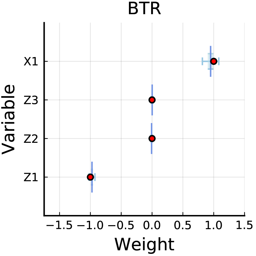
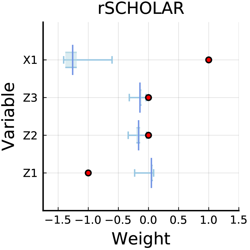
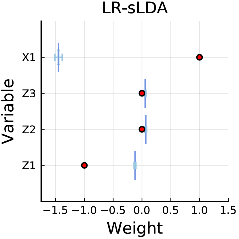
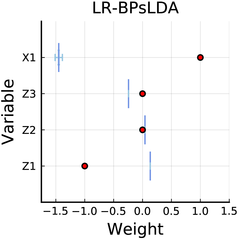
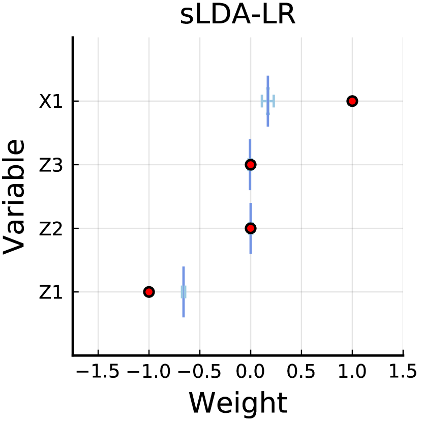
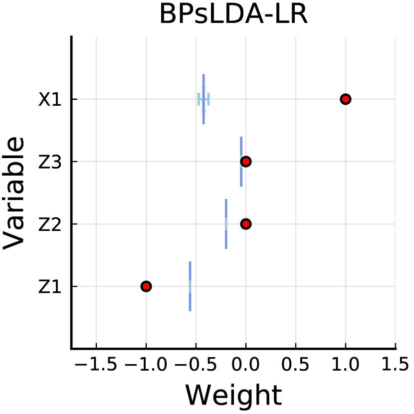
Figure 2: Comparing recovery of true regression weights across different topic models. For each panel, the true regression weights are shown as red points and the estimated $95\%$ posterior credible (or bootstrap, depending on model) interval in blue. Only BTR contains the true weights within the estimated intervals.

We generate $10,000$ documents of $50$ words each, following an LDA generative process, with each document having a distribution over three topics, defined over a vocabulary of 9 unique terms. A numerical feature, $\boldsymbol{x}=[x_{1},...,x_{D}]^{\intercal}$, is generated by calculating the document-level frequency of the first word in the vocabulary. As the first topic places a greater weight on the first three terms in the vocabulary, $\boldsymbol{x}$ is positively correlated with $\boldsymbol{\bar{z}}_{1}$. The response variable $\boldsymbol{y}=[y_{1},...,y_{D}]$ is generated through a linear combination of the numerical feature $\boldsymbol{x}$ and the average topic assignments $\boldsymbol{\bar{Z}}=\{\boldsymbol{\bar{z}}_{1},\boldsymbol{\bar{z}}_{2},\boldsymbol{\bar{z}}_{3}\}$,

$$\boldsymbol{y}=-\boldsymbol{\bar{z}}_{1}+\boldsymbol{x}+\boldsymbol{\epsilon}.$$ (18)

where $\boldsymbol{\epsilon}$ is an iid Gaussian white noise term. The regression model to recover the ground truth is then

$$\boldsymbol{y}=\omega_{1}\boldsymbol{\bar{z}}_{1}+\omega_{2}\boldsymbol{\bar{z}}_{2}+\omega_{3}\boldsymbol{\bar{z}}_{3}+\omega_{4}\boldsymbol{x}_{d}+\boldsymbol{\epsilon}.$$ (19)

The true regression weights are thus $\boldsymbol{\omega}^{*}=[-1,0,0,1]$. In accordance with the FWL theorem, we cannot recover the true coefficients with a two-stage estimation process.

5.2 Synthetic Data Results

We compare the ground truth of the synthetic data generating process against: (1) BTR: our Bayesian model, estimated via Gibbs sampling. (2) rSCHOLAR: the regression extension of SCHOLAR, estimated via neural VI. (3) LR-sLDA: first linearly regress $\boldsymbol{y}$ on $\boldsymbol{x}$, then use the residual of that regression as the response in an sLDA model, estimated via Gibbs sampling. (4) sLDA-LR: First sLDA, then linear regression. (5) BPsLDA-LR and (6) LR-BPsLDA: replace sLDA with BPsLDA, which is sLDA estimated via the backpropagation approach of Chen et al. (2015).

Figure 2 shows the true and estimated regression weights for each of the six models. LR-sLDA and sLDA-LR estimate inaccurate regression weights for both the text and numerical features, as do the BPsLDA variants. Similarly, rSCHOLAR fails to recover the ground truth. However, BTR estimates tight posterior distributions around to the true parameter values. The positive correlation between $\boldsymbol{z}_{1}$ and $\boldsymbol{x}$ makes a joint estimation approach crucial for recovering the true parameters. Standard supervised topic models estimate the regression parameters for the numerical features separately from the topic proportions and their associated regression parameters, violating the FWL theorem as outlined in section 2.2. A key difference between rSCHOLAR and BTR lies in their posterior estimation techniques (neural VI vs Gibbs). rSCHOLAR’s approach seems to have a similarly detrimental effect as the two-stage approaches. We suspect further research into (neural) VI assumptions and their effect on causal inference with text could be fruitful.

6 Experiment: Semi-Synthetic Data

6.1 Semi-Synthetic Data Generation

We further benchmark the models’ abilities to recover the ground truth on two semi-synthetic datasets. We still have access to the ground truth (GT) as we either synthetically create or directly observe the correlations between treatment, confounders and outcome. However, the text and some numeric metadata that we use is empirical. We use customer review data from (i) Booking.com and (ii) Yelp, and analyse two different ‘mock’ research questions. For both datasets, we randomly sample $50,000$ observations and select $75\%$ in Yelp, $80\%$ in Booking for training.
 
Booking: Do people give more critical ratings ($y_{i}$) to hotels that have high historic ratings ($av\_score_{i}$), once controlling for review texts?

$$GT_{B}:\quad y_{i}=-\text{hotel\_av}_{i}+5\text{prop\_pos}_{i}$$ (20)

where $\text{prop\_pos}_{i}$ is the proportion of positive words in a review. The textual effect is estimated via topic modelling in our experiment. The treatment in question is the average historic customer rating, being modelled as continuous.
 
Yelp: Do people from the US ($\text{US}_{i}$=1) give different Yelp ratings ($y_{i}$) than customers from Canada ($\text{US}_{i}$=0), controlling for average restaurant review ($\text{stars\_av\_b}_{i}$) and the review text?

$$GT_{Y}:y_{i}=-\text{US}_{i}+\text{stars\_av\_b}_{i}+sent_{i}.$$ (21)

To create the binary treatment variable $\text{US}_{i}$, we compute each review’s sentiment score ($sent_{i}$) using the Harvard Inquirer. This treatment effect is correlated with the text as

$$\Pr(US_{i}=1)=\frac{\exp(\gamma_{1}sent_{i})}{1+\exp(\gamma_{1}sent_{i})},$$ (22)

where $\gamma_{1}$ controls the correlation between text and treatment.

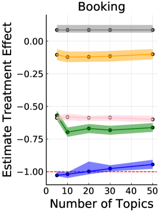
(a)

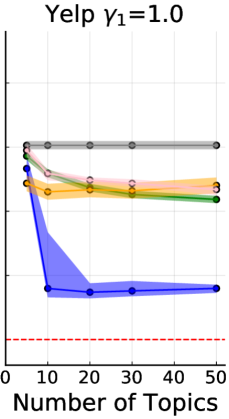
(b)

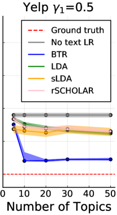
(c)

Figure 3: Estimated TE semi-synthetic Booking (left panel), Yelp (middle and right panel). Intervals are either 95% credible interval of posterior distribution, or based on 20 run bootstrap, depending on model.

6.2 Semi-Synthetic Data Results

On both semi-synthetic datasets and across all benchmarked models, BTR estimates the regression weights that are the closest to the ground truth. This consistently holds true across all tested numbers of topics $K$ (see Figure 3). For Yelp, we also vary the correlation strength between treatment and confounder. The middle panel in Figure 3 shows the estimation results with a very high correlation between confounder and treatment ($\gamma_{1}=1$). The RHS panel shows the results when this correlation is lower ($\gamma_{1}=0.5$). As expected, a higher correlation between confounder and treatment increases the bias as outlined in the section 2.2. If the correlation between confounder and treatment is zero, a two-stage estimation approach no longer violates FWL and all models manage to estimate the ground truth (see Appendix E). Since the topic modelling approach is an approximation to capture the true effect of the text and its correlation with the metadata - and since this approximation is not perfect - some bias may remain. Overall, BTR gets substantially closer to the ground truth than any other model.

7 Experiment: Real-World Data

Dataset	Booking
K	50	100
$pR^{2}$ (higher is better)
OLS	0.315
aRNN	0.479 (0.007)
LR+ TAM	0.479 (0.014)	0.487 (0.014)
LDA+LR	0.426 (0.003)	0.437 (0.002)
GSM+LR	0.386 (0.004)	0.395 (0.005)
LR+sLDA	0.432 (0.002)	0.438 (0.004)
LR+BPsLDA	0.419 (0.009)	0.455 (0.001)
LR+rSCHOLAR	0.469 (0.002)	0.465 (0.002)
rSCHOLAR	0.494 (0.004)	0.489 (0.003)
BTR	0.454 (0.003)	0.460 (0.002)
Perplexity (lower is better)
LR+TAM	521 (2)	522 (2)
LDA+LR	454 (1)	432 (1)
GSM+LR	369 (8)	348 (5)
LR+sLDA	436 (2)	411 (1)
LR+rSCHOLAR	441 (20)	458 (11)
rSCHOLAR	466 (19)	464 (9)
BTR	437 (1)	412 (1)

Table 1: Booking: mean $pR^{2}$ and perplexity, standard deviation in brackets. 20 model runs. Best model bold.

Dataset	Yelp
K	50	100
$pR^{2}$ (higher is better)
OLS	0.451
aRNN	0.582 (0.008)
LR+ TAM	0.585 (0.012)	0.587 (0.008)
LDA+LR	0.586 (0.006)	0.606 (0.007)
GSM+LR	0.495 (0.004)	0.517 (0.007)
LR+sLDA	0.571 (0.002)	0.574 (0.001)
LR+BPsLDA	0.603 (0.002)	0.609 (0.001)
LR+rSCHOLAR	0.550 (0.034)	0.557 (0.027)
rSCHOLAR	0.571 (0.01)	0.581 (0.009)
BTR	0.630 (0.001)	0.633 (0.001)
Perplexity (lower is better)
LR+TAM	1661 (7)	1655 (7)
LDA+LR	1306 (4)	1196 (2)
GSM+LR	1431 (34)	1387 (14)
LR+sLDA	1294 (5)	1174 (3)
LR+rSCHOLAR	1515 (34)	1516 (30)
rSCHOLAR	1491 (9)	1490 (9)
BTR	1291 (5)	1165 (3)

Table 2: Yelp: mean $pR^{2}$ and perplexity, standard deviation in brackets. 20 model runs. Best model bold.

The joint supervised estimation approach using text and non-text features, not only counteracts bias in causal settings. It also improves prediction performance. We use the real-world datasets of Booking and Yelp for our benchmarking. For both datasets, we predict customer ratings (response) for a business or hotel given customer reviews (text features) and business and customer metadata (numerical features).

7.1 Benchmarks

We add the following models to the benchmark list from the previous section: LDA+LR Griffiths and Steyvers (2004) and GSM+LR Miao et al. (2017) unsupervised Gibbs sampling and neural VI based topic models. LR+rSCHOLAR: the two-step equivalent for rSCHOLAR, estimating covariate regression weights in a separate step from the supervised topic model.

An alternative to topic based models are word-embedding based neural networks. We use (7) LR+aRNN: a bidirectional RNN with attention Bahdanau et al. (2015). Since the model does not allow for non-text features, we use the regression residuals of the linear regression as the target. And (8) LR+TAM: a bidirectional RNN using global topic vector to enhance its attention heads Wang and Yang (2020) - same target as in LR+aRNN.

7.2 Prediction and Perplexity Results

We evaluated all topic models on a range from 10 to 100 topics, with results for 50 and 100 in Table 2. Hyperparameters of benchmark models that have no direct equivalent in our model were set as suggested in the pertaining papers. We find that our results are robust across a wide range of hyperparameters (extensive robustness checks in Appendix G).

We assess the models’ predictive performance based on predictive $R^{2}$ ($pR^{2}=1-\frac{\text{MSE}}{var(y)}$). The upper part of Table 2 shows that BTR achieves the best $pR^{2}$ in the Yelp dataset and and very competitive results in the Booking dataset, where our rSCHOLAR extension outperforms all other models. Even the non-linear neural network models aRNN and TAM cannot achieve better results. Importantly, rSCHOLAR and BTR perform substantially better than their counterparts that do not jointly estimate the influence of covariates (LR+rSCHOLAR and LR+sLDA).

To assess document modelling performance, we report the test set perplexity score for all models that allow this (Table 2, bottom panel) . Perplexity is defined as $\exp\left\{-\frac{\sum^{D}_{d=1}\log p(\boldsymbol{w}_{d}|\boldsymbol{\theta},\boldsymbol{\beta})}{\sum_{d=1}^{D}N_{d}}\right\}$. The joint approach of both rSCHOLAR and BTR does not come at the cost of increased perplexity. If anything, the supervised learning approach using labels and covariates even improves document modelling performance when compared against its unsupervised counterpart (BTR vs LDA).

Assessing the interpretability of topic models is ultimately a subjective exercise. In Appendix G.4 we show topics associated with the most positive and negative regression weights, for each dataset. Overall, the identified topics and the sign of the associated weights seem interpretable and intuitive.

8 Conclusions

In this paper, we introduced BTR, a Bayesian topic regression framework that incorporates both numerical and text data for modelling a response variable, jointly estimating all model parameters. Motivated by the FWL theorem, this approach is designed to avoid potential bias in the regression weights, and can provide a sound regression framework for statistical and causal inference when one needs to control for both numerical and text based confounders in observational data. We demonstrate that our model recovers the ground truth with lower bias than any other benchmark model on synthetic and semi-synthetic datasets. Experiments on real-world data show that a joint and supervised learning strategy also yields superior prediction performance compared to ‘two-stage’ strategies, even competing with deep neural networks.

Appendix A Causal Inference with Text

For $D$ observations, we have outcome $\boldsymbol{y}\in\mathbb{R}^{D\times 1}$, treatment $\boldsymbol{t}\in\mathbb{R}^{D\times 1}$, text data $\boldsymbol{W}\in\mathbb{R}^{D\times V}$ (where $V$ is the vocabulary size) and numerical confounders $\boldsymbol{C}\in\mathbb{R}^{D\times P}$ (where $P$ is the number of numerical confounders).

As established in the main part of the paper, in order to estimate the ATT, we need to compute the conditional expectation function (CEF) $\mathbb{E}[\boldsymbol{y}|\boldsymbol{t},\boldsymbol{Z}]$ or if we have additional numerical confounders $\mathbb{E}[\boldsymbol{y}|\boldsymbol{t},\boldsymbol{Z},\boldsymbol{C}]$. Using regression to estimate our conditional expectation function, we can write

$$\mathbb{E}[\boldsymbol{y}|\boldsymbol{t},\boldsymbol{Z},\boldsymbol{C}]=f(\boldsymbol{t},\boldsymbol{Z},\boldsymbol{C};\boldsymbol{\Omega}).$$ (23)

Let $f()$ be the function of our regression equation that we need to define, and $\boldsymbol{\Omega}$ be the parameters of it. The predominant assumption in causal inference settings in many disciplines is a linear causal effect assumption. We follow this approach, also for the sake of simplicity. However, the requirement for joint supervised estimation of text representations $\boldsymbol{Z}$ to be able to predict $\boldsymbol{y}$,$\boldsymbol{t}$ (and if relevant $\boldsymbol{C}$) to be considered ‘causally sufficient’ is not constrained to the linear case Veitch et al. (2020). Under the linearity assumption, the CEF of our regression can take the form

$$\boldsymbol{y}=\mathbb{E}[\boldsymbol{y}|\boldsymbol{t},\boldsymbol{Z},\boldsymbol{C}]+\epsilon=\boldsymbol{t}\omega_{t}+\boldsymbol{Z}\boldsymbol{\omega_{Z}}+\boldsymbol{C}\boldsymbol{\omega_{C}}+\epsilon,$$ (24)

where $\epsilon\sim N(0,\sigma_{\epsilon}^{2})$ is additive iid Gaussian noise, ie. $\mathbb{E}[\epsilon|\boldsymbol{t},\boldsymbol{Z},\boldsymbol{C}]=0$ (see for example Angrist and Pischke (2008), chapter 3). Thus, $\sigma_{\epsilon}$ represents the conditional variance $Var(\boldsymbol{y}|\boldsymbol{t},\boldsymbol{Z},\boldsymbol{C})$. The regression approximates the CEF. Hence, when the CEF is causal, the regression estimates are causal Angrist and Pischke (2008). In such a case, $\omega_{t}$ measures the treatment effect. Assuming that $\boldsymbol{Z}$ and $\boldsymbol{C}$ block all ‘backdoor’ paths, the CEF would allow us to conduct causal inference of the ATT of $\boldsymbol{t}$ on $\boldsymbol{y}$ Pearl (2009).

We now shall revisit under which conditions, a decomposition of equation (24) into several separate estimation steps is permitted as described in the Frisch-Waugh-Lovell (or regression decomposition) theorem Lovell (2008), so that the regression estimates for $\omega_{t}$ remain unchanged and hence can still be considered as causal.

A.1 Regression Decomposition Theorem

The regression decomposition theorem or Frisch-Waugh-Lovell (FWL) theorem Frisch and Waugh (1933); Lovell (1963) states that the coefficients of a linear regression as stated in equation (24) are equivalent to the coefficients of partial regressions in which the residualized outcome is regressed on the residualized regressors - this residualization is in terms of all regressors that are not part of this partial regression.

For a moment, let us assume there are no confounding latent (that is to be estimated) text features $\boldsymbol{Z}$. Our observational data only consist of outcome $\boldsymbol{y}$, our treatment variable $\boldsymbol{t}$ and other observed confounding variables $\boldsymbol{C}$,

$$\boldsymbol{y}=\boldsymbol{t}\omega_{t}+\boldsymbol{C}\boldsymbol{\omega_{C}}+\epsilon.$$ (25)

The FWL theorem states that we would obtain mathematically identical regression coefficients $\omega_{t}$ and $\boldsymbol{\omega}_{C}$ is we decomposed this regression and estimated each part separately, each time residualizing (ie. orthogonalizing) outcomes and regressors on all other regressors.
 
More generally, for a linear regression define

$$\boldsymbol{y}=\boldsymbol{X}\boldsymbol{\beta}+\boldsymbol{\epsilon}$$

with $\boldsymbol{y}\in\mathbb{R}^{D\times 1}$, $\boldsymbol{\beta}\in\mathbb{R}^{K\times 1}$, $\boldsymbol{X}\in\mathbb{R}^{D\times M}$, which we could arbitrarily partition into $\boldsymbol{X}_{1}\in\mathbb{R}^{D\times K}$ and $\boldsymbol{X}_{2}\in\mathbb{R}^{D\times J}$ so we could also write

$$\boldsymbol{y}=\boldsymbol{X}_{1}\boldsymbol{\beta}_{1}+\boldsymbol{X}_{2}\boldsymbol{\beta}_{2}+\boldsymbol{\epsilon},$$

define projection (or prediction) matrix $\boldsymbol{P}$ such that

$$\boldsymbol{P}=\boldsymbol{X}(\boldsymbol{X}^{\intercal}\boldsymbol{X})^{-1}\boldsymbol{X}^{\intercal}.$$ (26)

$\boldsymbol{P}$ produces predictions $\boldsymbol{\widehat{y}}$ when applied to outcome vector $\boldsymbol{y}$,

$$\boldsymbol{\widehat{y}}=\boldsymbol{X}\boldsymbol{\widehat{\beta}}=\boldsymbol{X}(\boldsymbol{X}^{\intercal}\boldsymbol{X})^{-1}\boldsymbol{X}^{\intercal}\boldsymbol{y}=\boldsymbol{P}\boldsymbol{y}.$$ (27)

Also define the complement of $\boldsymbol{P}$, the residual maker matrix $\boldsymbol{M}$

$$\boldsymbol{M}=\boldsymbol{I}-\boldsymbol{P}=\boldsymbol{I}-\boldsymbol{X}(\boldsymbol{X}^{\intercal}\boldsymbol{X})^{-1}\boldsymbol{X}^{\intercal}$$ (28)

such that $\boldsymbol{M}$ applied to an outcome vector $\boldsymbol{y}$ yields

$$\boldsymbol{M}\boldsymbol{y}=\boldsymbol{y}-\boldsymbol{X}(\boldsymbol{X}^{\intercal}\boldsymbol{X})^{-1}\boldsymbol{X}^{\intercal}\boldsymbol{y}=\boldsymbol{y}-\boldsymbol{P}\boldsymbol{y}=\boldsymbol{y}-\boldsymbol{X}\boldsymbol{\widehat{\beta}}=\boldsymbol{\hat{\epsilon}}.$$ (29)

Theorem:
The FWL theorem states that equivalent to estimating

$$\boldsymbol{y}=\boldsymbol{X}_{1}\boldsymbol{\widehat{\beta}_{1}}+\boldsymbol{X}_{2}\boldsymbol{\widehat{\beta}_{2}}+\boldsymbol{\widehat{\epsilon}}$$ (30)

we would obtain mathematically identical regression coefficients $\boldsymbol{\widehat{\beta}_{1}}$ and $\boldsymbol{\widehat{\beta}_{2}}$ if we separately estimated

$$\boldsymbol{M}_{2}\boldsymbol{y} =\boldsymbol{M}_{2}\boldsymbol{X}_{1}\boldsymbol{\widehat{\beta}_{1}}+\boldsymbol{\hat{\epsilon}}$$ (31)

and

$$\boldsymbol{M}_{1}\boldsymbol{y} =\boldsymbol{M}_{1}\boldsymbol{X}_{2}\boldsymbol{\widehat{\beta}_{2}}+\boldsymbol{\hat{\epsilon}}$$ (32)

where $\boldsymbol{M}_{1}$ and $\boldsymbol{M}_{2}$ correspond to the data partitions $\boldsymbol{X}_{1}$ and $\boldsymbol{X}_{2}$.
 
Proof of Theorem:
This proof is based on the original papers Frisch and Waugh (1933); Lovell (1963). Given

$$\boldsymbol{y}=\boldsymbol{X}_{1}\boldsymbol{\widehat{\beta}_{1}}+\boldsymbol{X}_{2}\boldsymbol{\widehat{\beta}_{2}}+\boldsymbol{\widehat{\epsilon}}$$ (33)

left-multiply by $\boldsymbol{M}_{2}$, so we obtain

$$\boldsymbol{M}_{2}\boldsymbol{y}=\boldsymbol{M}_{2}\boldsymbol{X}_{1}\boldsymbol{\widehat{\beta}_{1}}+\boldsymbol{M}_{2}\boldsymbol{X}_{2}\boldsymbol{\widehat{\beta}_{2}}+\boldsymbol{M}_{2}\boldsymbol{\widehat{\epsilon}}.$$ (34)

We obtain from equation (28) that

$$\boldsymbol{M}_{2}\boldsymbol{X}_{2}\boldsymbol{\widehat{\beta}_{2}}=(\boldsymbol{I}-\boldsymbol{X}_{2}(\boldsymbol{X}_{2}^{\intercal}\boldsymbol{X}_{2})^{-1}\boldsymbol{X}_{2}^{\intercal})\boldsymbol{X}_{2}\boldsymbol{\widehat{\beta}_{2}}=\boldsymbol{X}_{2}\boldsymbol{\widehat{\beta}_{2}}-\boldsymbol{X}_{2}\boldsymbol{\widehat{\beta}_{2}}=\boldsymbol{0}.$$ (35)

Finally, $\boldsymbol{M}_{2}\boldsymbol{\hat{\epsilon}}=\boldsymbol{\hat{\epsilon}}$. $\boldsymbol{X}_{2}$ is orthogonal to $\boldsymbol{\epsilon}$ by construction of the OLS regression. Therefore, the residualized residuals are the residuals themselves. Which leaves us with

$$\boldsymbol{M}_{2}\boldsymbol{y}=\boldsymbol{M}_{2}\boldsymbol{X}_{1}\boldsymbol{\widehat{\beta}_{2}}+\boldsymbol{\hat{\epsilon}}\qed.$$ (36)

The same goes through for $\boldsymbol{M}_{1}$ by analogy.

A.2 $\mathbb{E}[\boldsymbol{y}|\boldsymbol{t},\boldsymbol{C}]$, where $\boldsymbol{t}\perp\boldsymbol{C}$, no $\boldsymbol{Z}$

In the simplest case assume there was no confounding text. Our observational data only consist of outcome $\boldsymbol{y}$, our treatment variable $\boldsymbol{t}$ and other potential confounding variables $\boldsymbol{C}$. The conditional expectation function is $\mathbb{E}[\boldsymbol{y}|\boldsymbol{t},\boldsymbol{C}]$. We can estimate it via one joint regression as

$$\boldsymbol{y}=\boldsymbol{t}\omega_{t}+\boldsymbol{C}\omega_{C}+\epsilon_{0}.$$ (37)

Now, assuming that the linearity assumption is correct, the fact that $\boldsymbol{t}\perp\boldsymbol{C}$ implies that $\boldsymbol{C}$ is not actually a confounder in this setup. We would obtain the exact same regression coefficient estimates for $\omega_{t}$ and $\boldsymbol{\omega}_{C}$ if we followed a two-step process, in which we first regress $\boldsymbol{y}$ on $\boldsymbol{t}$

$$\boldsymbol{y}=\boldsymbol{t}\omega_{t}+\epsilon_{1}.$$ (38)

$$\boldsymbol{y}=\boldsymbol{C}\omega_{C}+\epsilon_{1}.$$ (39)

This is holds only true, if and only if $\boldsymbol{t}\perp\boldsymbol{C}$. Because in this case, $\boldsymbol{t}$ and $\boldsymbol{C}$ are already orthorgonal to each other. They already fulfill the requirements of the FWL and therefore such two-step process would yield mathematically equivalent regression coefficients $\boldsymbol{\omega}$ to the joint estimation in equation (37). Put in terms of the conditional expectations, given linearity, $\mathbb{E[\boldsymbol{y}|\boldsymbol{t},\boldsymbol{C}}]=\mathbb{E[\boldsymbol{y}|\boldsymbol{t}}]+\mathbb{E[\boldsymbol{y}|\boldsymbol{C}}]$, since $\boldsymbol{t}$ and $\boldsymbol{C}$ are uncorrelated and therefore $\boldsymbol{C}$ is not an actual confounder under the linear CEF setup.

A.3 $\mathbb{E}[\boldsymbol{y}|\boldsymbol{t},\boldsymbol{C}]$, where $\boldsymbol{t}\not\perp\boldsymbol{C}$, no $\boldsymbol{Z}$

In this case, $\boldsymbol{t}\not\perp\boldsymbol{C}$. We now have $\mathbb{E[\boldsymbol{y}|\boldsymbol{t},\boldsymbol{C}}]\neq\mathbb{E[\boldsymbol{y}|\boldsymbol{t}}]$ in the linear CEF setup, since $\boldsymbol{C}$ is a confounder. However, according to the FWL, we can still conduct separate stage regressions and obtain mathematically equivalent regression coefficients $\boldsymbol{\omega}$ if we residualize outcomes and regressors on all regressors that are not part of the partial regression. We can estimate

$$\boldsymbol{M}_{C}\boldsymbol{y}=\boldsymbol{M}_{C}\boldsymbol{t}\boldsymbol{\widehat{\omega}_{t}}+\boldsymbol{\hat{\epsilon}_{1}}$$ (40)

and

$$\boldsymbol{M}_{t}\boldsymbol{y}=\boldsymbol{M}_{t}\boldsymbol{C}\boldsymbol{\widehat{\omega}_{C}}+\boldsymbol{\hat{\epsilon}_{2}}$$ (41)

and the obtained estimates $\widehat{\omega_{t}}$ and $\boldsymbol{\widehat{\omega}_{C}}$ will be equivalent to those obtained from the joint estimation.

A.4 $\mathbb{E}[\boldsymbol{y}|\boldsymbol{t},\boldsymbol{C},\boldsymbol{Z}]$, where $\boldsymbol{t}\not\perp\boldsymbol{C}$,$\boldsymbol{Z}$

We now consider the case where part (or all) of our confounders are text or where text is a proxy for otherwise unobserved confounders. The joint estimation would be

$$\boldsymbol{y}=\boldsymbol{t}\boldsymbol{\widehat{\omega}_{t}}+\boldsymbol{C}\boldsymbol{\widehat{\omega}_{C}}+\boldsymbol{Z}\boldsymbol{\widehat{\omega}_{Z}}+\boldsymbol{\hat{\epsilon}}$$ (42)

where $\boldsymbol{Z}$ itself is obtain through supervised learning via text representation function

$$\boldsymbol{Z}=g(\boldsymbol{W},\boldsymbol{y},\boldsymbol{t},\boldsymbol{C};\Theta).$$

We therefore cannot decompose this joint estimation into separate parts. As long as the text features $\boldsymbol{Z}$ are correlated with the outcome and the other covariates, we would need to apply the orthogonalization via the respective $\boldsymbol{M}$ matrices for each partical regression. Since $\boldsymbol{Z}$ needs to be estimated itself (it is ‘estimated data’), we cannot residualize on $\boldsymbol{Z}$ though. Nor can $\boldsymbol{Z}$ be residualized on the other covariates. A separate-stage approach will therefore lead to biased estimates of $\boldsymbol{\omega}$.

Appendix B Regression Model

Due to the conjugacy of the Normal-Inverse-Gamma prior, the posterior distribution of the regression parameters conditional on $\boldsymbol{A}$ has a known Normal-Inverse-Gamma distribution:

$$p(\boldsymbol{\omega},\sigma^{2}| \boldsymbol{y},\boldsymbol{A})\propto p(\boldsymbol{\omega}|\sigma^{2},\boldsymbol{y},\boldsymbol{A})p(\sigma^{2}\mid\boldsymbol{y},\boldsymbol{A})=\mathcal{N}\left(\boldsymbol{\omega}|\boldsymbol{m}_{n},\sigma^{2}\boldsymbol{S}_{n}^{-1}\right){\mathcal{IG}}\left(\sigma^{2}|a_{n},b_{n}\right)$$ (43)

where $\boldsymbol{m}_{n}$, $\boldsymbol{S}_{n}$, $a_{n}$ and $b_{n}$ follow standard updating equations for a Bayesian Linear Regression (Bishop 2006)

$$\boldsymbol{m}_{n}=(\boldsymbol{A}^{\intercal}\boldsymbol{A}+\boldsymbol{S}_{0})^{-1}(\boldsymbol{S}_{0}\boldsymbol{m}_{0}+\boldsymbol{A}^{\intercal}\boldsymbol{y})$$ (44)

$$\boldsymbol{S}_{n}=(\boldsymbol{A}^{\intercal}\boldsymbol{A}+\boldsymbol{S}_{0})$$ (45)

$$a_{n}=a_{0}+N/2$$ (46)

$$b_{n}=b_{0}+\left(\boldsymbol{y}^{\intercal}\boldsymbol{y}+\boldsymbol{m}_{0}^{\intercal}\boldsymbol{S}_{0}\boldsymbol{m}_{0}-\boldsymbol{m}_{n}^{\intercal}\boldsymbol{S}_{n}\boldsymbol{m}_{n}\right)/2.$$ (47)

Appendix C Topic Model

C.1 Gibbs-EM algorithm

C.1.1 Sampling distribution for $z$

The probability of a given word $w_{d,n}$ being assigned to a given topic $k$ (such that $z_{d,n}=k$), conditional on the assignments of all other words (as well as the model’s other latent variables and the data) is

$$p(z_{d,n}=k|\boldsymbol{Z}_{-(d,n)},\boldsymbol{W},\boldsymbol{X},\boldsymbol{y},\boldsymbol{\omega},\sigma^{2}),$$ (48)

where $\boldsymbol{Z}_{-(d,n)}$ are the topic assignments for all words apart from $w_{d,n}$. By the conditional independence properties implied by the graphical model, we can split this joint posterior into

$$p(\boldsymbol{Z}|\boldsymbol{W},\boldsymbol{X},\boldsymbol{y},\boldsymbol{\omega},\sigma^{2})\propto p(\boldsymbol{Z}|\boldsymbol{W})p(\boldsymbol{y}|\boldsymbol{Z},\boldsymbol{X},\boldsymbol{\omega},\sigma^{2}).$$ (49)

As topic assignments within one document are independent from topic assignments in all other documents, the sampling equation for the $n$th word in document $d$ should only depend it’s own response variable, $y_{d}$, such that

$$p(z_{d,n}=k|\boldsymbol{Z}_{-(d,n)},\boldsymbol{W},\boldsymbol{X},\boldsymbol{y},\boldsymbol{\omega},\sigma^{2})\propto p(z_{d,n}=k|\boldsymbol{Z}_{-(d,n)},\boldsymbol{W})p(y_{d}|z_{d,n}=k,\boldsymbol{Z}_{-(d,n)},\boldsymbol{x}_{d},\boldsymbol{\omega},\sigma^{2}).$$ (50)

The first part of the RHS expression is just the sampling distribution of a standard LDA model, so it can be expressed in terms of the count variables $\boldsymbol{s}$ (the topic assignments across a document) and $\boldsymbol{m}$ (the assignments of unique words across topics over all documents). $s_{d,k}$ measures the total number of words in document $d$ assigned to topic $k$ and $s_{d,k,-n}$ the number of words in document $d$ assigned to topic $k$, except for word $n$. Analogously, $m_{k,v}$ measures the total number of times term $v$ is assigned to topic $k$ across all documents and $m_{k,v,-(d,n)}$ measures the same, but excludes word $n$ in document $d$.

$$p(z_{d,n}=k|\boldsymbol{Z}_{-(d,n)},\boldsymbol{W})\propto(s_{d,k,-n}+\alpha)\frac{m_{k,v,-(d,n)}+\eta}{\sum_{v}m_{k,v,-(d,n)}+V\eta}.$$ (51)

C.1.2 Regression

Given that the residuals are Gaussian, the probability of the response variable for a given document $d$ is

$$p(y_{d}|\boldsymbol{z}_{d},\boldsymbol{x}_{d},\boldsymbol{\omega},\sigma^{2})=\frac{1}{\sqrt{2\pi\sigma^{2}}}\exp\left\{-\frac{(y_{d}-\boldsymbol{\omega}^{\intercal}\boldsymbol{a}_{d})^{2}}{2\sigma^{2}}\right\}.$$ (52)

We can write this in a convenient form that preserves proportionality with respect to $z_{d,n}$ such that it depends only on the data and count variables used in the other two terms. First, we split the $\boldsymbol{x}_{d}$ features into those that are interacted, $\boldsymbol{x}_{1,d}$, and those that are not, $\boldsymbol{x}_{2,d}$. The generative model for $y_{d}$ is then

$$y_{d}\sim\mathcal{N}(\boldsymbol{\omega}_{z}^{\intercal}\boldsymbol{\bar{z}}_{d}+\boldsymbol{\omega}_{zx}^{\intercal}(\boldsymbol{x}_{1,d}\otimes\boldsymbol{\bar{z}}_{d})+\boldsymbol{\omega}_{x}^{\intercal}\boldsymbol{x}_{2,d},\sigma^{2}).$$ (53)

where $\otimes$ is the Kronecker product. Noting that $\boldsymbol{X}$ is observed, so we can think of this as a linear model with document-specific regression parameters. Define $\boldsymbol{\tilde{\omega}}_{z,d}$ as a length $K$ vector such that

$$\tilde{\omega}_{z,d,k}=\omega_{z,k}+\boldsymbol{\omega}_{zx,k}^{\intercal}\boldsymbol{x}_{1,d}.$$ (54)

Noting that $\boldsymbol{\tilde{\omega}}_{z,d}^{\intercal}\boldsymbol{\bar{z}}_{d}=\frac{\boldsymbol{\tilde{\omega}_{z,d}}^{\intercal}}{N_{d}}(\boldsymbol{s}_{d,-n}+\boldsymbol{s}_{d,n})$, the probability density of $y$ conditional on $z_{d,n}=k$ is therefore proportional to

$$p(y_{d}|z_{d,n}=k,\boldsymbol{z}_{-(d,n)},\boldsymbol{x}_{d},\boldsymbol{\omega},\sigma^{2})\propto$$

$$\exp\left\{\frac{1}{2\sigma^{2}}\left(\frac{2\tilde{\omega}_{z,d,k}}{N_{d}}\left(y_{d}-\boldsymbol{\omega}_{x}^{\intercal}\boldsymbol{x}_{d}-\frac{\boldsymbol{\tilde{\omega}}_{z,d}^{\intercal}}{N_{d}}\boldsymbol{s}_{d,-n}\right)-\left(\frac{\tilde{\omega}_{z,d,k}}{N_{d}}\right)^{2}\right)\right\}.$$ (55)

This gives us the sampling distribution for $z_{d,n}$ stated in equation (50): a multinomial distribution parameterised by

$$p(z_{d,n}=k|\boldsymbol{Z}_{-(d,n)},\boldsymbol{W},\boldsymbol{X},\boldsymbol{y},\alpha,\eta,\boldsymbol{\omega},\sigma^{2})\propto$$

$$(s_{d,k,-n}+\alpha)\frac{m_{k,v,-(d,n)}+\eta}{\sum_{v}m_{k,v,-(d,n)}+V\eta}$$

$$\exp\left\{\frac{1}{2\sigma^{2}}\left(\frac{2\tilde{\omega}_{z,d,k}}{N_{d}}\left(y_{d}-\boldsymbol{\omega}_{x}^{\intercal}\boldsymbol{x}_{2,d}-\frac{\boldsymbol{\tilde{\omega}}_{z,d}^{\intercal}}{N_{d}}\boldsymbol{s}_{d,-n}\right)-\left(\frac{\tilde{\omega}_{z,d,k}}{N_{d}}\right)^{2}\right)\right\}.$$ (56)

This defines for each $k\in\{1,...,K\}$ the probability that $z_{d,n}$ is assigned to that topic. These $K$ probabilities define the multinomial distribution from which $z_{d,n}$ is drawn.

C.1.3 $\theta$ and $\beta$

Given topic assignments $z$, we can recover the latent variables $\theta$ and $\beta$ from their predictive distributions via

$$\hat{\theta}_{d,k}=\frac{s_{d,k}+\alpha}{\sum_{k}(s_{d,k}+\alpha)}$$ (57)

and

$$\hat{\beta}_{k,v}=\frac{m_{k,v}+\eta}{\sum_{v}(m_{k,v}+\eta)}.$$ (58)

C.1.4 Observations without documents

A straightforward extension allows for some observations to be associated with an $\boldsymbol{X}$ and $\boldsymbol{y}$, but no document. This is often the case in a social science context, for example time-series may be associated with documents at irregular intervals. If an observation is not associated with any documents, the priors on the document topic distributions suggest that the topic assignment for topic $K$ is set to $\alpha_{k}/\sum_{k}\alpha_{k}$. These observations may still be very useful in estimating the relationship between $\boldsymbol{X}$ and $\boldsymbol{y}$ so they are worth including in the estimation.

C.1.5 Multiple paragraphs

If, as is often the case in the context of social science applications, we have relatively few observations but the documents associated with those observations are relatively long, we can exploit the structure of the documents by estimating the model at a paragraph level. Splitting up longer documents into paragraphs brings one of the key advantages of topic modelling to the fore: that the same word can have different meanings in different contexts. For example, the word “increase" might have quite a different meaning if it is in a paragraph with the word “risk" than if it is alongside “productivity". Treating the entire document as a single bag of words makes it hard for the model to make this distinction.
 
If there are observations with multiple documents, we can treat these as $P_{d}$ separate paragraphs of a combined document, indexed by $p$, each with an independent $\boldsymbol{\theta}_{p}$ distribution over topics. These paragraphs may also have different associated $\boldsymbol{x}_{d,p}$ that interact with the topics, for example we may wish to interact topics with a paragraph specific sentiment score, but the response variable $y_{d}$ is common to all paragraphs in the same document and the M-step estimated at the document level. Figure 4 shows the extended graphical model.

Figure 4: Graphical model for BTR with multiple documents per observation

If $\boldsymbol{x_{d,p}}$ only enters linearly into the regression then some document-level average will have to be used and this transformation can be performed prior to estimation, converting it into an $\boldsymbol{x}_{1,d}$, and so the algorithm will remain unchanged. However, if any of the $\boldsymbol{x}_{d,p}$ variables are interacted with $\boldsymbol{\bar{z}}_{d,p}$ then we may wish for this interaction to be at the paragraph level. For example, if we think that a topic might have a different effect depending on the sentiment of the surrounding paragraph. In this case, we still need to aggregate the interaction to the document level, but aggregate after interacting rather than interacting after aggregating. We therefore define

$$\overline{\boldsymbol{x}_{d,p}\otimes\boldsymbol{z}_{d,p}}=\frac{1}{N_{d}}\sum_{p\in[P_{d}]}\sum_{n\in[N_{d,p}]}\left[\boldsymbol{x}_{d,p}\otimes\boldsymbol{s}_{d,p,n}\right]$$ (59)

where $[N]$ denotes the set of integers $\{1,...,N\}$ and $\otimes$ represents the Kronecker product. The design matrix $\boldsymbol{A}$ is then

$$\boldsymbol{A}=\left[\begin{matrix}\boldsymbol{\bar{z_{1}}}&\overline{\boldsymbol{x}_{1,1,p}\otimes\boldsymbol{z}_{1,p}}&\boldsymbol{x}_{2,1}\\ \vdots&\vdots&\vdots\\ \boldsymbol{\bar{z}}_{1}&\overline{\boldsymbol{x}_{1,d,p}\otimes\boldsymbol{z}_{d,p}}&\boldsymbol{x}_{2,d}\\ \vdots&\vdots&\vdots\\ \boldsymbol{\bar{z}}_{1}&\overline{\boldsymbol{x}_{1,D,p}\otimes\boldsymbol{z}_{D,p}}&\boldsymbol{x}_{2,D}\\ \end{matrix}\right]$$ (60)

and the predictive model for $y_{d}$ will be

$$\boldsymbol{y}\sim\mathcal{N}(\boldsymbol{A}\boldsymbol{\omega},\sigma^{2})\ \ \text{where}\ \ \boldsymbol{\omega}=(\boldsymbol{\omega}_{z},\boldsymbol{\omega}_{zx},\boldsymbol{\omega}_{x}).$$ (61)

The simplest way to aggregate from paragraphs to documents is simply to give each word in the document equal weight as above. This will mean that longer paragraphs have greater weight than shorter ones.
 
As before, we can collapse out the latent variables $\boldsymbol{\theta}$ and $\boldsymbol{\beta}$ so that we only need to sample for the topic assignments $\boldsymbol{z}$ in an E-step and then for $\boldsymbol{\omega}$ and $\sigma^{2}$ in an M-step.
 
In the E-step, we need to sample from the conditional posterior for the topic assignment of each word

$$\Pr[z_{d,p,n}=k|\boldsymbol{Z}_{d,-(p,n)},\boldsymbol{W},\alpha,\eta,\boldsymbol{y},\boldsymbol{X},\boldsymbol{\omega},\sigma^{2}].$$ (62)

By the conditional independence properties of the graphical model, we can split this into $p(\boldsymbol{Z}|\boldsymbol{W},\alpha,\eta)$ and $p(\boldsymbol{y}|\boldsymbol{Z},\boldsymbol{X},\boldsymbol{\omega},\sigma^{2})$. The sampling equation for the $n$th token in the $p$th paragraph of the $d$th document $d$ will have the form

$$\begin{split}\Pr[z_{d,p,n}=k|\boldsymbol{Z}_{d,-(p,n)},\boldsymbol{W},\alpha,\eta,\boldsymbol{y},\boldsymbol{X},\boldsymbol{\omega},\sigma^{2}]\propto&\\ \Pr[z_{d,p,n}=k|\boldsymbol{Z}_{d,p,-(n)},\boldsymbol{W},\alpha,\eta]&\ \ \times\ \ \Pr[y_{d}|z_{d,p,n}=k,\boldsymbol{Z}_{d,-(p,n)},\boldsymbol{x}_{d},\omega,\sigma^{2}].\end{split}$$ (63)

The topic assignment each document is independent, but there are dependencies across paragraphs. Crucially, these paragraphs have are independent with respect to $\boldsymbol{\theta}$, so $p(\boldsymbol{Z}|\boldsymbol{W},\alpha,\eta)$ is paragraph specific.

$$\Pr[z_{d,p,n}=k|\boldsymbol{Z}_{d,p-(n)},\boldsymbol{W},\alpha,\eta]\propto(s_{d,p,k,-n}+\alpha)\frac{m_{k,v,-(d,p,n)}+\eta}{\sum_{v}m_{k,v,-(d,p,n)}+V\eta}.$$ (64)

However, the regression part is at the document level to $p(\boldsymbol{y}|\boldsymbol{Z},\boldsymbol{X},\boldsymbol{\omega},\sigma^{2})$ will condition on all the paragraphs in a given document. Given that the residuals are Gaussian, the probability of the outcome variable for a given document $d$ is

$$p(\boldsymbol{y}_{d}|\boldsymbol{z}_{d},\boldsymbol{x}_{d},\boldsymbol{\omega},\sigma^{2})=\frac{1}{\sqrt{2\pi\sigma^{2}}}\exp\left[-\frac{(y_{d}-\boldsymbol{\omega}_{z}^{\intercal}\boldsymbol{\bar{z}}_{d}-\boldsymbol{\omega}_{zx}^{\intercal}(\overline{\boldsymbol{x}_{1,d,p}\otimes\boldsymbol{z}_{d,p}})-\boldsymbol{\omega}_{x}^{\intercal}\boldsymbol{x}_{2,d})^{2}}{2\sigma^{2}}\right].$$ (65)

We can write this in a convenient form that preserves proportionality with respect to $z_{d,p,n}$ such that it depends only on the data and count variables used in the other two terms and the document-wide counts. First we can break the prediction for $y_{d}$ into the section that depends on paragraph $p$ and the section that depends on other paragraphs and document wide $\boldsymbol{x}_{1,d}$.

$$\begin{split}y_{d}-\boldsymbol{\omega}_{z}^{\intercal}\boldsymbol{\bar{z}}_{d}-\boldsymbol{\omega}_{zx}^{\intercal}(\overline{\boldsymbol{x}_{1,d,p}\otimes\boldsymbol{z}_{d,p}})=&\left(y_{d}-\boldsymbol{\omega}_{x}^{\intercal}\boldsymbol{x}_{2,d}-\frac{\boldsymbol{\omega}_{z}^{\intercal}}{N_{d}}\boldsymbol{s}_{d,-p}-\frac{\boldsymbol{\omega}_{zx}^{\intercal}}{N_{d}}\sum_{q\in\{[P_{d}]\backslash p\}}\left[\boldsymbol{x}_{1,d,q}\otimes\boldsymbol{s}_{d,q}\right]\right)\\ &-\left(\frac{\boldsymbol{\omega}_{z}^{\intercal}}{N_{d}}(\boldsymbol{s}_{d,p,-n}+\boldsymbol{s}_{d,p,n})-\frac{\boldsymbol{\omega}_{zx}^{\intercal}}{N_{d}}\boldsymbol{x}_{1,d,p}\otimes(\boldsymbol{s}_{d,p,-n}+\boldsymbol{s}_{d,p,n})\right)\end{split}$$ (66)

where $N_{d}$ is the total number of words in the document.
 
Define $\hat{y}_{d,-p}$ as the predicted $y_{d}$ without paragraph $p$,

$$\hat{y}_{d,-p}=\boldsymbol{\omega}_{x}^{\intercal}\boldsymbol{x}_{2,d}+\frac{\boldsymbol{\omega}_{z}^{\intercal}}{N_{d}}\boldsymbol{s}_{d,-p}+\frac{\boldsymbol{\omega}_{zx}^{\intercal}}{N_{d}}\sum_{q\in\{[P_{d}]\backslash p\}}\left[\boldsymbol{x}_{1,d,q}\otimes\boldsymbol{s}_{d,q}\right].$$ (67)

We then have a predictive distribution that depends only on paragraph $p$.

$$y_{d}\sim\mathcal{N}\left(\hat{y}_{d,-p}-\frac{\boldsymbol{\omega}_{z}^{\intercal}}{N_{d}}(\boldsymbol{s}_{d,p,-n}+\boldsymbol{s}_{d,p,n})-\frac{\boldsymbol{\omega}_{zx}^{\prime}}{N_{d}}\boldsymbol{x}_{1,d,p}\otimes(\boldsymbol{s}_{d,p,-n}+\boldsymbol{s}_{d,p,n}),\sigma^{2}\right).$$ (68)

We can then follow the same steps as for the single paragraph document case to derive the third term in the sampling distribution, defining $\boldsymbol{\tilde{\omega}}_{z,d,p,k}=\boldsymbol{\omega}_{z,k}+\boldsymbol{\omega}_{zx,k}^{\prime}\boldsymbol{x}_{1,d,p}$ analogously to $\boldsymbol{\tilde{\omega}}$ defined for the single paragraph case.
 
This gives us the sampling distribution for $z$, which is a Multinomial parameterised by

$$\begin{split}\Pr[z_{d,n}=k|\boldsymbol{Z}_{-(d,n)},\boldsymbol{W},\boldsymbol{y},\alpha,\eta,\boldsymbol{\omega},\sigma^{2}]\propto&(s_{d,p,k,-n}+\alpha)\frac{m_{k,v,-(d,p,n)}+\eta}{\sum_{v}m_{k,v,-(d,p,n)}+V\eta}\\ &\exp\left[\frac{1}{2\sigma^{2}}\left(\frac{2\tilde{\omega}_{z,d,p,k}}{N_{d}}\left(y_{d}-\hat{y}_{d,-p}-\frac{\boldsymbol{\tilde{\omega}}_{z,d,p}^{\prime}}{N_{d}}\boldsymbol{s}_{d,-n}\right)-\left(\frac{\tilde{\omega}_{z,d,p,k}}{N_{d}}\right)\right)^{2}\right].\end{split}$$ (69)

In the M-step we can then still use the average $\bar{z}_{d,p}$ estimated in the E-step, but we need to weight each paragraph by the number of words in that paragraph to be consistent with the E-step,

$$\bar{z}_{d}=\frac{1}{N_{d}}\sum_{p\in[P_{d}]}\left[N_{d,p}\bar{z}_{d,p}\right]$$ (70)

$$(\overline{x_{1,d,p}\otimes z_{d,p}})=\frac{1}{N_{d}}\sum_{p\in[P_{d}]}\left[N_{d,p}x_{1,d,p}\otimes z_{d,p}\right].$$ (71)

Appendix D Synthetic Data Experiments

Figure 5 shows the topic-vocabulary distribution from which the synthetic documents are generated.

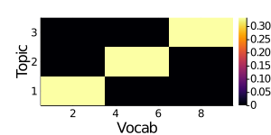
Figure 5: Ground truth topic distribution for synthetic documents.

Table 3 shows the hyperparameter settings used in the synthetic data section. We observed that the settings of the prior did hardly effect results, given the strong signal in the synthetic dataset.

Table 3: Synthetic example hyperparameters

	K	$\alpha$	$\eta$	$\mu_{\text{ntm}}$	$\sigma_{\text{ntm}}$	$a_{0}$	$b_{0}$	$m_{0}$	$S_{0}$
LDA	3	1.0	1.0	-	-	-	-	-	-
sLDA	3	1.0	1.0	-	-	-	-	-	-
BPsLDA	3	1.0	1.0	-	-	-	-	-	-
BTR	3	1.0	1.0	-	-	0.2	4	0	2

Appendix E Semi-Synthetic Data Experiments

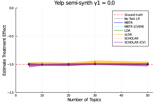
Figure 6: Without correlation between confounders and treatments, the regression can be dissected into two separate parts (supervised topic estimation and regression weight estimation of the non-text features) without inducing bias in the estimators, as described in the section on the Frisch-Waugh-Lovell theorem. In such a case, all models manage to recover the ground truth.

Appendix F Real-World Datasets and Data Pre-Processing

The Yelp dataset contains over $8$ million customer reviews of businesses, which we restrict to reviews for businesses in Toronto. The Booking dataset contains around $500,000$ hotel reviews. For both datasets, we randomly sample $50,000$ observations and randomly select $75\%$ in Yelp, $80\%$ in Booking of our sample for training, holding out the remainder for testing. We then further split the training set equally for training in the E-step and validation in the M-step. The features are normalized on the training data statistics and the response variable is de-meaned. We do this because the $K$ topic features sum to one and therefore implicitly already add a constant to the regression (Blei and McAuliffe, 2008). We preprocess the text corpora by removing stopwords and then tokenizing and stemming the data.

Table 4: Summary statistics of the review datasets

Statistics	#train	#val	#test	#vocab	#max words	#avg words
Yelp	18,750	18,750	12,500	24,680	572	61.2
Booking	20,000	20,000	10,000	6,968	305	18.7

The Booking.com dataset allows consumers to enter the positive and negative parts of their reviews in separate boxes. We combine these two reviews for all our exercises, but we do use information on the word count in each of these sections (see below).
 
For the prediction exercises in Section 7, we use the number of stars associated with each review as the target variable. We also use the numerical metadata described in Table 5as covariates.

Table 5: Numerical covariates for prediction experiments

Dataset	Variable	Description
Yelp	stars_av_u	historic avg. rating by user
	stars_av_b	historic avg. rating of business
	sentiment	Harvard Inquirer sentiment score
Booking	Average_Score	historical avg. hotel score
	Review_Total_Negative_Word_Counts	total number of words in the negative part of review
	Review_Total_Positive_Word_Counts	total number of words in the positive part of review
	Total_Number_of_Reviews_Reviewer_Has_Given	total num of reviews by customer
	Total_Number_of_Reviews	total num of reviews of hotel

For the semi-synthetic exercise on the Booking data, we construct

$$pos\_prop_{i}=\frac{Review\_Total\_Positive\_Word\_Counts_{i}}{Review\_Total\_Positive\_Word\_Counts_{i}+Review\_Total\_Negative\_Word\_Counts_{i}}$$

This variable is correlated with the treatment ($Average\_Score_{i}$) and with the outcome, and so the text can act as a confounder.

Appendix G Real-World Data Experiments

G.1 Empirical data evaluation across different K

Table 6: Mean $pR^{2}$ and perplexity over 20 runs per model, standard deviation in brackets

Dataset	Booking				Yelp
K	10	20	30	50	10	20	30	50
$pR^{2}$ (higher is better)
LDA+LR	0.400 (0.003)	0.410 (0.004)	0.417 (0.005)	0.426 (0.003)	0.498 (0.005)	0.530 (0.009)	0.561 (0.010)	0.586 (0.006)
GSM+LR	0.387 (0.003)	0.390 (0.004)	0.389 (0.006)	0.386 (0.004)	0.502 (0.013)	0.505 (0.011)	0.503 (0.008)	0.495 (0.004)
LR+sLDA	0.416 (0.007)	0.426 (0.003)	0.430 (0.004)	0.432 (0.002)	0.533 (0.007)	0.564 (0.003)	0.567 (0.006)	0.571 (0.002)
LR+BPsLDA	0.394 (0.004)	0.396 (0.005)	0.400 (0.005)	0.419 (0.009)	0.593 (0.003)	0.597 (0.002)	0.597 (0.002)	0.603 (0.002)
rSCHOLAR	0.494 (0.005)	0.495 (0.003)	0.495 (0.003)	0.494 (0.004)	0.520 (0.02)	0.548 (0.02)	0.563 (0.01)	0.571 (0.01)
BTR	0.439 (0.008)	0.447 (0.005)	0.453 (0.003)	0.454 (0.003)	0.586 (0.007)	0.615 (0.006)	0.627 (0.004)	0.630 (0.001)
Perplexity (lower is better)
LDA+LR	538 (3)	498 (2)	476 (2)	454 (1)	1544 (5)	1447 (4)	1388 (4)	1306 (4)
GSM+LR	371 (6)	359 (11)	356 (14)	369 (8)	1500 (52)	1444 (29)	1463 (21)	1431 (34)
LR+sLDA	535 (2)	491 (1)	463 (1)	436 (2)	1544 (6)	1444 (6)	1382 (5)	1294 (5)
rSCHOLAR	941 (134)	1429 (163)	2110 (396)	5014 (1314)	1744 (158)	1918 (138)	2216 (164)	2814 (383)
BTR	535 (2)	490 (1)	463 (2)	437 (1)	1540 (5)	1443 (4)	1379 (4)	1291 (5)

Table 7: Best model in bold. Second best model in italics.

We also tested sLDA+LR and a pure sLDA, which performed consistently worse so they are not included for the sake of brevity. For example, for $K=50$, sLDA+LR achieved $pR^{2}$ of $0.420$ and $0.564$ for Booking and Yelp respectively, compared to $0.432$ and $0.571$ for LR+sLDA. Standalone sLDA achieves $0.356$ and $0.526$ respectively.

G.2 Model parametrisations

This section provides an overview over all used and tested hyperparameter settings across all models in our benchmark list. Table 8 lists all hyperparameter settings pertaining to topic model components. Table 9 provides an overview over all used neural network hyperparameters. 10 summarises the iteration and stopping criteria for all models.

Table 8: Topic model hyperparameters

	K	$\alpha$	$\eta$	$\mu_{\text{ntm}}$	$\sigma_{\text{ntm}}$	$a_{0}$	$b_{0}$	$m_{0}$	$S_{0}$
LDA	[10,20,30,50]	[0.1,0.5,1]	[0.001,0.01,0.1]	-	-	-	-	-	-
sLDA	[10,20,30,50]	[0.1,0.5,1]	[0.001,0.01,0.1]	-	-	-	-	-	-
BPsLDA	[10,20,30,50]	[0.1,0.5,1]	[0.001,0.01,0.1]	-	-	-	-	-	-
BTR	[10,20,30,50,100]	[0.1,0.5,1]	[0.001,0.01,0.1]	-	-	[0,1.5,3,4]	[0,2,4]	0	2
GSM	[10,20,30,50]	-	-	0	1	-	-	-	-
TAM	100	-	-	0	1	-	-	-	-
Bold parameter specifications were used for reported results in paper, unless stated otherwise. For Booking default $a_{0}=3$, for Yelp $a_{0}=4$.

Table 9: Neural network hyperparameters

	HidLaySize			DropOut		HidLaySize		nHidLayers
	$\theta$	BatchSize	LearnRate	KeepRate	EmbedSize	RNN	TAM-thresh	BPsLDA
GSM	64	64	1.00E-03	[0.5,0.8,1]*	-	-	-	-
TAM	64	64	1.00E-03	0.8	100	64	1/K	-
aRNN	-	64	1.00E-03	0.8	100	64	-	-
BPsLDA	-	1050	1.00E-02	-	-	-	-	10
* best results (which occurred under no dropout) were reported in benchmarks

Table 10: Iteration parameters

	E-step iters	M-step iters	max. EM-iters	burn-in	max. epochs	Gibbs iters (thinning)
LDA	-	-	50***	100	-	1000 (5)
sLDA	[100,250,500]**	2500	50***	20	-	-
BTR	[100,250,500]**	2500	50***	20	-	-
GSM	-	-	-	-	100***	-
TAM	-	-	-	-	100***	-
BPsLDA	-	-	-	-	50***	-
** no noticeable performance difference observed, therefore all results reported based on 100 E-step.
*** best model achieved substantially before max. iterations reached.

Further notes on benchmark model specifications:
 
For TAM and aRNN, the sequence length in the RNN component (ie. the maximum number of words per document) is $305$ for Booking and $572$ for Yelp which corresponds to the longest review in each respective data set. We therefore work with the full text of each review.

BPsLDA changes its behaviour quite drastically when $\alpha$ is set in an area $1\leq\alpha\leq 2$, where it strongly increases its predictive performance ($pR^{2}$) at the cost of its document modelling performance (perplexity). This can be seen in the original paper Chen et al. (2015). We included $\alpha=1$ in the robustness test range and BTR is still generally on par with BPsLDA in this specific case for low $K$ and does better for $K>30$. Even when including $\alpha=1$ in the robustness test range, BTR still outperforms BPsLDA and all other models across all hyperparameter settings, except $K=10$ in the Yelp dataset, where BTR is a close second.

G.3 Robustness Tests

Robustness test across all topic models with LDA-like structure and Dirichlet hyperparameters for document-topic and word-topic distributions.

We assess the robustness of our findings to changes in the Dirichlet hyperparameters $\alpha$ and $\eta$. These hyperparameters act as priors on the topic-document distributions ($\boldsymbol{\beta}$) and word-topic distributions ($\boldsymbol{\theta}$), respectively. Table 11 shows the results.

In terms of $pR^{2}$, BTR continues to perform best for all settings. We generally find that the BTR prediction performance is robust to hyperparameter changes. Evaluating the perplexity scores, we see more fluctuation across all models, which is unsurprising since those hyperparameter directly affect the generative topic modelling processes. BTR remains on par with its sLDA counterpart.

Table 11: Sensitivity to hyperparameters $\alpha$ and $\beta$ (K = 20)

		$\alpha$			$\eta$
Metric	Model	0.1	0.5	1	0.001	0.01	0.1
Yelp $pR^{2}$	LR-LDA	0.473	0.530	0.550	0.316	0.530	0.521
	LR-sLDA	0.558	0.564	0.559	0.562	0.564	0.568
	LR-BPsLDA	0.602	0.597	0.608	0.607	0.597	0.608
	BTR	0.611	0.615	0.613	0.611	0.615	0.624
Yelp perplexity	LR-LDA	1511	1448	1445	1472	1447	1470
	LR-sLDA	1497	1444	1431	1441	1444	1491
	BTR	1490	1443	1441	1456	1443	1478
Booking $pR^{2}$	LR-LDA	0.397	0.410	0.409	0.405	0.410	0.406
	LR-sLDA	0.430	0.426	0.432	0.422	0.426	0.433
	LR-BPsLDA	0.409	0.396	0.453	0.395	0.396	0.393
	BTR	0.451	0.447	0.452	0.443	0.447	0.455
Booking perplexity	LR-LDA	515	498	514	505	498	512
	LR-sLDA	502	491	504	484	491	516
	BTR	503	491	503	489	491	515

G.3.1 Further Robustness Tests - Booking

Table 12 provides an extended robustness test on the predictive performance of the benchmark topic models across hyperparameters. BTR continues to be the best performing model throughout. Table 13 summarises robustness tests in terms of perplexity scores. BTR achieves almost identical perplexity scores as sLDA whilst achieving higher $pR^{2}$ throughout.

Table 12: Booking - $pR^{2}$ for different hyperparameter settings across topic benchmark models, best model in bold.

(K=10)	$\alpha$ = 0.1	$\alpha$ = 0.5	$\alpha$ = 1	$\eta$ = 0.001	$\eta$ = 0.01	$\eta$ = 0.1	a,b = (3,2)	a,b = (0,0)	a,b = (3,4)	a,b = (1.5,4)
LR-LDA	0.378	0.4	0.408	0.397	0.4	0.398
LR-sLDA	0.42	0.416	0.403	0.401	0.416	0.422
LR-BPsLDA	0.396	0.394	0.439	0.393	0.394	0.396
BTR	0.446	0.439	0.435	0.418	0.439	0.452	0.439	0.435	0.437	0.446
(K=20)	$\alpha$ = 0.1	$\alpha$ = 0.5	$\alpha$ = 1	$\eta$ = 0.001	$\eta$ = 0.01	$\eta$ = 0.1	a,b = (3,2)	a,b = (0,0)	a,b = (3,4)	a,b = (1.5,4)
LR-LDA	0.397	0.41	0.409	0.405	0.41	0.406
LR-sLDA	0.43	0.426	0.432	0.422	0.426	0.433
LR-BPsLDA	0.409	0.396	0.453	0.395	0.396	0.393
BTR	0.451	0.447	0.452	0.443	0.447	0.455	0.447	0.45	0.45	0.443
(K=30)	$\alpha$ = 0.1	$\alpha$ = 0.5	$\alpha$ = 1	$\eta$ = 0.001	$\eta$ = 0.01	$\eta$ = 0.1	a,b = (3,2)	a,b = (0,0)	a,b = (3,4)	a,b = (1.5,4)
LR-LDA	0.399	0.417	0.423	0.417	0.417	0.413
LR-sLDA	0.434	0.43	0.428	0.417	0.43	0.427
LR-BPsLDA	0.424	0.4	0.451	0.401	0.4	0.402
BTR	0.455	0.453	0.455	0.444	0.453	0.459	0.453	0.453	0.447	0.449
(K=50)	$\alpha$ = 0.1	$\alpha$ = 0.5	$\alpha$ = 1	$\eta$ = 0.001	$\eta$ = 0.01	$\eta$ = 0.1	a,b = (3,2)	a,b = (0,0)	a,b = (3,4)	a,b = (1.5,4)
LR-LDA	0.415	0.426	0.428	0.418	0.426	0.420
LR-sLDA	0.434	0.432	0.43	0.429	0.432	0.436
LR-BPsLDA	0.461	0.419	0.449	0.411	0.419	0.418
BTR	0.461	0.454	0.459	0.446	0.454	0.459	0.454	0.455	0.452	0.451
Default model was $\alpha=0.5$, $\eta=0.01$, $a_{0}=3$, $b_{0}=2$.
Robustness tests kept all hyperparameters at default, then changing one hyperparameter at a time.

Table 13: Booking - perplexity scores for different hyperparameter settings across topic benchmark models, best model in bold.

K=10	$\alpha$ = 0.1	$\alpha$ = 0.5	$\alpha$ = 1	$\eta$ = 0.001	$\eta$ = 0.01	$\eta$ = 0.1	a,b = (3,2)	a,b = (0,0)	a,b = (3,4)	a,b = (1.5,4)
LDA	562	538	539	539	538	545
LR-sLDA	557	535	539	534	535	554
BTR	556	535	538	528	535	548	535	535	537	536
K=20	$\alpha$ = 0.1	$\alpha$ = 0.5	$\alpha$ = 1	$\eta$ = 0.001	$\eta$ = 0.01	$\eta$ = 0.1	a,b = (3,2)	a,b = (0,0)	a,b = (3,4)	a,b = (1.5,4)
LDA	515	498	514	505	498	512
LR-sLDA	502	491	504	484	491	516
BTR	503	490	503	489	490	515	490	491	490	491
K=30	$\alpha$ = 0.1	$\alpha$ = 0.5	$\alpha$ = 1	$\eta$ = 0.001	$\eta$ = 0.01	$\eta$ = 0.1	a,b = (3,2)	a,b = (0,0)	a,b = (3,4)	a,b = (1.5,4)
LDA	479	476	502	484	476	492
LR-sLDA	471	463	486	454	463	499
BTR	470	463	483	457	463	500	463	463	463	463
K=50	$\alpha$ = 0.1	$\alpha$ = 0.5	$\alpha$ = 1	$\eta$ = 0.001	$\eta$ = 0.01	$\eta$ = 0.1	a,b = (3,2)	a,b = (0,0)	a,b = (3,4)	a,b = (1.5,4)
LDA	442	454	494	460	454	476
LR-sLDA	431	436	466	421	436	492
BTR	430	437	467	423	437	492	437	436	439	437
Default model was $\alpha=0.5$, $\eta=0.01$, $a_{0}=3$, $b_{0}=2$.
Robustness tests kept all hyperparameters at default, then changing one hyperparameter at a time.

G.3.2 Further Robustness Tests - Yelp

Table 14 provides an extended robustness test on the predictive performance of the benchmark topic models across hyperparameters. BTR continues to be the best performing model throughout, apart from the K=10 case, where it is a close second. Table 15 summarises robustness tests in terms of perplexity scores. BTR achieves almost identical perplexity scores as sLDA whilst achieving higher $pR^{2}$ throughout.

Table 14: Yelp - $pR^{2}$ for different hyperparameter settings across topic benchmark models, best model in bold.

K=10	$\alpha$ = 0.1	$\alpha$ = 0.5	$\alpha$ = 1	$\eta$ = 0.001	$\eta$ = 0.01	$\eta$ = 0.1	a,b = (4,2)	a,b = (0,0)	a,b = (3,4)	a,b = (1.5,4)
LR-LDA	0.476	0.498	0.515	0.503	0.498	0.49
LR-sLDA	0.523	0.533	0.539	0.52	0.533	0.527
LR-BPsLDA	0.596	0.593	0.606	0.595	0.593	0.592
BTR	0.592	0.586	0.593	0.575	0.586	0.596	0.586	0.588	0.578	0.59
K=20	$\alpha$ = 0.1	$\alpha$ = 0.5	$\alpha$ = 1	$\eta$ = 0.001	$\eta$ = 0.01	$\eta$ = 0.1	a,b = (4,2)	a,b = (0,0)	a,b = (3,4)	a,b = (1.5,4)
LR-LDA	0.473	0.53	0.55	0.483	0.53	0.521
LR-sLDA	0.558	0.564	0.559	0.562	0.564	0.568
LR-BPsLDA	0.602	0.597	0.608	0.607	0.597	0.608
BTR	0.611	0.615	0.613	0.611	0.615	0.624	0.615	0.62	0.593	0.621
K=30	$\alpha$ = 0.1	$\alpha$ = 0.5	$\alpha$ = 1	$\eta$ = 0.001	$\eta$ = 0.01	$\eta$ = 0.1	a,b = (4,2)	a,b = (0,0)	a,b = (3,4)	a,b = (1.5,4)
LR-LDA	0.499	0.561	0.563	0.547	0.561	0.565
LR-sLDA	0.565	0.567	0.563	0.567	0.567	0.56
LR-BPsLDA	0.609	0.597	0.607	0.599	0.597	0.599
BTR	0.624	0.627	0.612	0.608	0.627	0.622	0.627	0.623	0.627	0.626
K=50	$\alpha$ = 0.1	$\alpha$ = 0.5	$\alpha$ = 1	$\eta$ = 0.001	$\eta$ = 0.01	$\eta$ = 0.1	a,b = (4,2)	a,b = (0,0)	a,b = (3,4)	a,b = (1.5,4)
LR-LDA	0.523	0.586	0.591	0.571	0.586	0.582
LR-sLDA	0.573	0.571	0.564	0.556	0.571	0.573
LR-BPsLDA	0.612	0.603	0.606	0.604	0.603	0.604
BTR	0.632	0.630	0.623	0.621	0.630	0.632	0.630	0.629	0.629	0.628

Table 15: Yelp - perplexity scores for different hyperparameter settings across topic benchmark models, best model in bold.

K=10	$\alpha$ = 0.1	$\alpha$ = 0.5	$\alpha$ = 1	$\eta$ = 0.001	$\eta$ = 0.01	$\eta$ = 0.1	a,b = (4,2)	a,b = (0,0)	a,b = (3,4)	a,b = (1.5,4)
LDA	1586	1544	1532	1557	1544	1552	1544
LR-sLDA	1583	1544	1530	1561	1544	1554	1544
BTR	1588	1540	1534	1565	1540	1546	1540	1539	1548	1547
K=20	$\alpha$ = 0.1	$\alpha$ = 0.5	$\alpha$ = 1	$\eta$ = 0.001	$\eta$ = 0.01	$\eta$ = 0.1	a,b = (4,2)	a,b = (0,0)	a,b = (3,4)	a,b = (1.5,4)
LDA	1511	1447	1445	1472	1447	1469	1447
LR-sLDA	1497	1444	1431	1441	1444	1491	1444
BTR	1490	1443	1441	1456	1443	1478	1443	1443	1445	1441
K=30	$\alpha$ = 0.1	$\alpha$ = 0.5	$\alpha$ = 1	$\eta$ = 0.001	$\eta$ = 0.01	$\eta$ = 0.1	a,b = (4,2)	a,b = (0,0)	a,b = (3,4)	a,b = (1.5,4)
LDA	1434	1388	1390	1412	1388	1415	1388
LR-sLDA	1436	1382	1383	1395	1382	1442	1382
BTR	1434	1379	1385	1390	1379	1448	1379	1378	1389	1379
K=50	$\alpha$ = 0.1	$\alpha$ = 0.5	$\alpha$ = 1	$\eta$ = 0.001	$\eta$ = 0.01	eta = 0.1	a,b = (4,2)	a,b = (0,0)	a,b = (3,4)	a,b = (1.5,4)
LDA	1352	1306	1325	1334	1306	1356	1306
LR-sLDA	1349	1294	1310	1309	1294	1404	1294
BTR	1338	1291	1303	1288	1291	1405	1291	1293	1294	1292

G.4 Estimated Topics

The below tables are an extended version of the corresponding table in the paper. The show the top $3$ negative and positive topics for $K=[10,30,100]$. Inspecting the top words in each of these topics compared with its regression coefficient, BTR models highly interpretable topics - at least as interpretable as LDA or sLDA. At the same time BTR achieves substantially better prediction performances throughout all model specifications (see previous section).

Table 16: Top 3 positive and negative topics for Yelp (K = 10)

	Pos1	Pos2	Pos3	Neg3	Neg2	Neg1
BTR topics	food	restaur	time	store	food	order
	great	dish	hair	locat	chicken	us
	place	lobster	back	like	good	ask
	servic	menu	work	can	order	servic
	friend	food	will	price	rice	wait
	love	order	day	go	dish	food
BTR regr. weights	4.3	1.7	1.5	-0.1	-0.5	-8.8
sLDA topics	food	time	locat	coffe	us	like
	place	hair	store	tea	order	place
	great	back	can	tri	ask	go
	servic	work	find	place	servic	much
	good	will	place	ice	tabl	im
	time	day	staff	cream	time	realli
sLDA regr. weights	2.7	1.7	1.2	0.1	-3.7	-4.5
LDA topics	food	place	place	store	fri	order
	great	coffe	great	like	burger	us
	servic	good	good	locat	order	food
	restaur	tri	friend	can	like	servic
	dish	tea	bar	find	good	time
	menu	great	drink	go	chees	ask
LDA regr. weights	1.2	0.7	0.5	-0.1	-0.4	-2.6

Table 17: Top 3 positive and negative topics for Yelp (K = 30)

	Pos1	Pos2	Pos3	Neg3	Neg2	Neg1
BTR topics	best	great	restaur	us	ask	like
	plac	friend	menu	order	said	disappoint
	alway	servic	dish	tabl	custom	better
	love	staff	wine	food	told	tast
	ever	recommend	steak	server	never	noth
	toronto	amaz	perfect	came	say	bad
BTR regr. weights	6.9	6.0	2.1	-3.9	-8.4	-13.3
sLDA topics	great	time	im	seem	ask	like
	love	alway	review	like	never	food
	amaz	go	place	much	custom	good
	recommend	year	star	make	said	place
	servic	never	go	think	servic	tast
	friend	everi	give	thing	told	better
sLDA regr. weights	3.7	3.1	3.1	-2.3	-6.4	-7.1
LDA topics	great	toronto	restaur	us	ask	like
	friend	visit	menu	tabl	custom	tast
	love	make	dish	order	said	disappoint
	amaz	love	wine	food	servic	better
	place	made	dessert	came	told	bad
	servic	best	dinner	server	manag	noth
LDA regr. weights	3.0	1.6	1.3	-1.2	-4.9	-8.3

Table 18: Top 3 positive and negative topics for Yelp (K = 100)

	Pos1	Pos2	Pos3	Neg3	Neg2	Neg1
BTR topics	love	definit	best	custom	never	disappoint
	delici	ever	amaz	ask	worst	tast
	definit	toronto	everi	said	ever	bland
	perfect	citi	friend	manag	money	dri
	tri	far	free	rude	bad	better
	super	amaz	alway	servic	terribl	lack
BTR regr. weights	5.9	5.2	5.0	-8.4	-12.5	-14.5
sLDA topics	alway	will	amaz	ask	tast	disappoint
	time	definit	definit	said	like	bad
	usual	servic	love	told	felt	cold
	come	friend	great	back	disappoint	worst
	never	return	place	went	better	dri
	everi	back	everyth	want	wasnt	lack
sLDA regr. weights	4.1	4.0	3.9	-7.0	-8.0	-11.3
LDA topics	love	best	experi	money	never	tast
	amaz	toronto	made	go	bad	like
	delici	ever	make	will	ever	disappoint
	place	citi	feel	never	worst	meat
	absolut	far	first	pay	terribl	bland
	super	visit	felt	spend	experi	dri
LDA regr. weights	5.4	4.6	3.8	-5.9	-10.8	-10.9

Table 19: Top 3 positive and negative topics for Booking (K = 10)

	Pos1	Pos2	Pos3	Neg3	Neg2	Neg1
BTR topics	hotel	room	room	room	check	hotel
	stay	locat	great	bed	book	room
	staff	staff	love	shower	room	locat
	would	good	hotel	bathroom	us	small
	help	clean	view	small	hotel	good
	everyth	comfort	bar	clean	arriv	price
BTR regr. weights	2.8	1.7	1.5	-1.0	-1.1	-5.7
sLDA topics	hotel	room	room	room	room	room
	stay	good	great	bed	night	hotel
	staff	locat	love	bathroom	window	locat
	would	staff	hotel	shower	work	small
	help	clean	view	small	floor	staff
	like	breakfast	nice	comfort	air	posit
sLDA regr. weights	2.4	1.3	1.3	-0.4	-0.6	-5.6
LDA topics	hotel	hotel	neg	check	room	room
	stay	great	staff	room	shower	hotel
	staff	love	locat	book	bathroom	good
	help	room	friendli	hotel	work	locat
	would	view	great	us	bed	breakfast
	noth	locat	help	time	air	price
LDA regr. weights	1.3	1.2	1.0	-1.3	-1.4	-2.0

Table 20: Top 3 positive and negative topics for Booking (K = 30)

	Pos1	Pos2	Pos3	Neg3	Neg2	Neg1
BTR topics	us	stay	room	room	ask	room
	staff	would	locat	small	us	hotel
	made	hotel	great	bed	day	old
	upgrad	staff	staff	size	recept	poor
	stay	love	bit	locat	call	star
	welcom	recommend	littl	bathroom	back	bad
BTR regr. weights	2.7	2.5	2.3	-2.5	-3.0	-9.0
sLDA topics	staff	hotel	us	book	room	hotel
	friendli	love	upgrad	charg	need	room
	great	beauti	staff	hotel	locat	bad
	help	decor	room	pay	old	star
	locat	modern	stay	check	look	poor
	neg	great	love	day	smell	posit
sLDA regr. weights	2.1	1.8	1.7	-1.4	-2.1	-9.7
LDA topics	stay	stay	hotel	us	room	hotel
	hotel	hotel	love	ask	locat	like
	made	would	beauti	one	good	star
	like	recommend	great	recept	need	realli
	feel	definit	decor	day	old	much
	realli	love	staff	call	valu	best
LDA regr. weights	2.4	2.1	1.9	-2.5	-2.7	-3.4

Table 21: Top 3 positive and negative topics for Booking (K = 100)

	Pos1	Pos2	Pos3	Neg3	Neg2	Neg1
BTR topics	staff	hotel	love	old	room	poor
	help	wonder	great	look	small	posit
	friendli	beauti	staff	carpet	tini	servic
	excel	love	littl	tire	bathroom	bad
	especi	experi	fab	furnitur	noisi	never
	wonder	fabul	especi	need	far	rude
BTR regr. weights	4.3	4.1	3.3	-6.1	-7.3	-14.2
sLDA topics	love	room	great	old	hotel	bad
	beauti	small	locat	dirti	star	poor
	amaz	posit	neg	bathroom	expect	recept
	fantast	size	perfect	carpet	rate	posit
	fabul	bit	awesom	wall	thi	even
	wonder	expect	super	look	basic	never
sLDA regr. weights	3.7	3.6	2.8	-5.8	-6.0	-14.3
LDA topics	love	great	bit	hotel	old	recept
	amaz	locat	littl	star	dirti	manag
	everyth	neg	nice	rate	carpet	rude
	noth	staff	locat	expect	look	receptionist
	perfect	awesom	breakfast	disappoint	wall	check
	absolut	perfect	good	thi	furnitur	guest
LDA regr. weights	3.6	3.1	2.8	-5.3	-6.6	-7.6

G.5 Computation Times

Table 22 shows the time taken for 100 E-step iterations on a single 2.8GHz processor on the Booking data and 300-400 seconds on the Yelp data. We found that 100 E-step iterations is typically sufficient for the best performance and the model typically converges after between 10-25 EM iterations. A typical 30 topic model on Yelp data thus took around 1 hour to converge, and around 20 minutes for Booking. Computation time scales roughly linearly in the number of topics and total number of words across all documents. This is because the evaluation of the $K$-dimensional multinomial distribution for each $z_{d,n}$ (equation (50)) is the principle computational challenge.

Table 22: Computational time

Dataset	K	100 E-step iters
Yelp	10	50s
	20	110s
	30	200s
	50	320s
	100	740s
Booking	10	18s
	20	33s
	30	50s
	50	79s
	100	200s

Note: Yelp data has roughly 3 times as many words as Booking.com data

References

- Angrist and Pischke (2008) Joshua D Angrist and Jörn-Steffen Pischke. 2008. Mostly harmless econometrics: An empiricist’s companion. Princeton University Press.
- Bahdanau et al. (2015) Dzmitry Bahdanau, Kyunghyun Cho, and Yoshua Bengio. 2015. Neural machine translation by jointly learning to align and translate. In 3rd International Conference on Learning Representations, ICLR.
- Bishop (2006) Christopher M Bishop. 2006. Pattern recognition and machine learning. Information Science and Statistics. Springer, New York.
- Blei et al. (2017) David M Blei, Alp Kucukelbir, and Jon D McAuliffe. 2017. Variational inference: A review for statisticians. Journal of the American Statistical Association, 112(518):859–877.
- Blei and McAuliffe (2008) David M Blei and Jon D McAuliffe. 2008. Supervised topic models. In Advances in Neural Information Processing Systems, pages 121–128.
- Blei et al. (2003) David M Blei, Andrew Y Ng, and Michael I Jordan. 2003. Latent dirichlet allocation. Journal of Machine Learning Research, 3(Jan):993–1022.
- Card et al. (2018) Dallas Card, Chenhao Tan, and Noah A. Smith. 2018. Neural models for documents with metadata. In Proceedings of the 56th Annual Meeting of the Association for Computational Linguistics (Volume 1: Long Papers), pages 2031–2040. Association for Computational Linguistics.
- Chen et al. (2015) Jianshu Chen, Ji He, Yelong Shen, Lin Xiao, Xiaodong He, Jianfeng Gao, Xinying Song, and Li Deng. 2015. End-to-end learning of lda by mirror-descent back propagation over a deep architecture. In Advances in Neural Information Processing Systems, volume 28.
- Egami et al. (2018) Naoki Egami, Christian J Fong, Justin Grimmer, Margaret E Roberts, and Brandon M Stewart. 2018. How to make causal inferences using texts. arXiv preprint arXiv:1802.02163.
- Eisenstein et al. (2011) Jacob Eisenstein, Amr Ahmed, and Eric P Xing. 2011. Sparse additive generative models of text. In Proceedings of the 28th international conference on machine learning (ICML-11), pages 1041–1048. Citeseer.
- Fong and Grimmer (2016) Christian Fong and Justin Grimmer. 2016. Discovery of treatments from text corpora. In Proceedings of the 54th Annual Meeting of the Association for Computational Linguistics (Volume 1: Long Papers), pages 1600–1609, Berlin, Germany. Association for Computational Linguistics.
- Frisch and Waugh (1933) Ragnar Frisch and Frederick V Waugh. 1933. Partial time regressions as compared with individual trends. Econometrica: Journal of the Econometric Society, pages 387–401.
- Gentzkow et al. (2019) Matthew Gentzkow, Bryan Kelly, and Matt Taddy. 2019. Text as data. Journal of Economic Literature, 57(3):535–74.
- Griffiths and Steyvers (2004) Thomas L. Griffiths and Mark Steyvers. 2004. Finding scientific topics. Proceedings of the National Academy of Sciences, 101(suppl 1):5228–5235.
- Grimmer and Stewart (2013) Justin Grimmer and Brandon M Stewart. 2013. Text as data: The promise and pitfalls of automatic content analysis methods for political texts. Political analysis, 21(3):267–297.
- Keith et al. (2020) Katherine Keith, David Jensen, and Brendan O’Connor. 2020. Text and causal inference: A review of using text to remove confounding from causal estimates. In Proceedings of the 58th Annual Meeting of the Association for Computational Linguistics, pages 5332–5344, Online. Association for Computational Linguistics.
- Kingma and Ba (2015) Diederik P. Kingma and Jimmy Ba. 2015. Adam: A method for stochastic optimization. In 3rd International Conference on Learning Representations, ICLR, Conference Track Proceedings.
- Kingma and Welling (2014) Diederik P. Kingma and Max Welling. 2014. Auto-encoding variational bayes. In 2nd International Conference on Learning Representations, ICLR, Conference Track Proceedings.
- Levine and Casella (2001) Richard A Levine and George Casella. 2001. Implementations of the monte carlo em algorithm. Journal of Computational and Graphical Statistics, 10(3):422–439.
- Lovell (1963) Michael C Lovell. 1963. Seasonal adjustment of economic time series and multiple regression analysis. Journal of the American Statistical Association, 58(304):993–1010.
- Lovell (2008) Michael C Lovell. 2008. A simple proof of the fwl theorem. The Journal of Economic Education, 39(1):88–91.
- Magnusson et al. (2020) Måns Magnusson, Leif Jonsson, and Mattias Villani. 2020. Dolda: a regularized supervised topic model for high-dimensional multi-class regression. Computational Statistics, 35(1):175–201.
- Miao et al. (2017) Yishu Miao, Edward Grefenstette, and Phil Blunsom. 2017. Discovering discrete latent topics with neural variational inference. In International Conference on Machine Learning, pages 2410–2419. PMLR.
- Mozer et al. (2020) Reagan Mozer, Luke Miratrix, Aaron Russell Kaufman, and L. Jason Anastasopoulos. 2020. Matching with text data: An experimental evaluation of methods for matching documents and of measuring match quality. Political Analysis, 28(4):445–468.
- Pearl (2009) Judea Pearl. 2009. Causality (2nd edition). Cambridge University Press.
- Rezende et al. (2014) Danilo Jimenez Rezende, Shakir Mohamed, and Daan Wierstra. 2014. Stochastic backpropagation and approximate inference in deep generative models. In Proceedings of the 31st International Conference on Machine Learning, volume 32 of Proceedings of Machine Learning Research, pages 1278–1286, Bejing, China. PMLR.
- Robert and Casella (2013) Christian Robert and George Casella. 2013. Monte Carlo statistical methods. Springer Science & Business Media.
- Roberts et al. (2016) Margaret E Roberts, Brandon M Stewart, and Edoardo M Airoldi. 2016. A model of text for experimentation in the social sciences. Journal of the American Statistical Association, 111(515):988–1003.
- Roberts et al. (2020) Margaret E Roberts, Brandon M Stewart, and Richard A Nielsen. 2020. Adjusting for confounding with text matching. American Journal of Political Science, 64(4):887–903.
- Shinozaki and Ostendorf (2007) Takahiro Shinozaki and Mari Ostendorf. 2007. Cross-validation em training for robust parameter estimation. In IEEE International Conference on Acoustics, Speech and Signal Processing-ICASSP, volume 4, pages IV–437.
- Stuart et al. (1994) Alan Stuart, Steven Arnold, J Keith Ord, Anthony O’Hagan, and Jonathan Forster. 1994. Kendall’s advanced theory of statistics. Wiley.
- Tan et al. (2014) Chenhao Tan, Lillian Lee, and Bo Pang. 2014. The effect of wording on message propagation: Topic- and author-controlled natural experiments on Twitter. In Proceedings of the 52nd Annual Meeting of the Association for Computational Linguistics (Volume 1: Long Papers), pages 175–185, Baltimore, Maryland. Association for Computational Linguistics.
- Veitch et al. (2020) Victor Veitch, Dhanya Sridhar, and David Blei. 2020. Adapting text embeddings for causal inference. In Conference on Uncertainty in Artificial Intelligence, pages 919–928. PMLR.
- Wang and Yang (2020) Xinyi Wang and Yi Yang. 2020. Neural topic model with attention for supervised learning. In International Conference on Artificial Intelligence and Statistics, pages 1147–1156. PMLR.
- Wang and Zhu (2014) Yining Wang and Jun Zhu. 2014. Spectral methods for supervised topic models. In Advances in Neural Information Processing Systems, pages 1511–1519.
- Wood-Doughty et al. (2018) Zach Wood-Doughty, Ilya Shpitser, and Mark Dredze. 2018. Challenges of using text classifiers for causal inference. In Proceedings of the Conference on Empirical Methods in Natural Language Processing. Conference on Empirical Methods in Natural Language Processing, volume 2018, page 4586. NIH Public Access.
- Zhu et al. (2012) Jun Zhu, Amr Ahmed, and Eric P Xing. 2012. Medlda: maximum margin supervised topic models. Journal of Machine Learning Research, 13(Aug):2237–2278.