JigSaw: Boosting Fidelity of NISQ Programs
via Measurement Subsetting
Abstract.
Near-term quantum computers contain noisy devices, which makes it difficult to infer the correct answer even if a program is run for thousands of trials. On current machines, qubit measurements tend to be the most error-prone operations (with an average error-rate of 4%) and often limit the size of quantum programs that can be run reliably on these systems. As quantum programs create and manipulate correlated states, all the program qubits are measured in each trial and thus, the severity of measurement errors increases with the program size. The fidelity of quantum programs can be improved by reducing the number of measurement operations.
We present JigSaw, a framework that reduces the impact of measurement errors by running a program in two modes. First, running the entire program and measuring all the qubits for half of the trials to produce a global (albeit noisy) histogram. Second, running additional copies of the program and measuring only a subset of qubits in each copy, for the remaining trials, to produce localized (higher fidelity) histograms over the measured qubits. JigSaw then employs a Bayesian post-processing step, whereby the histograms produced by the subset measurements are used to update the global histogram. Our evaluations using three different IBM quantum computers with 27 and 65 qubits show that JigSaw improves the success rate on average by 3.6x and up-to 8.4x. Our analysis shows that the storage and time complexity of JigSaw scales linearly with the number of qubits and trials, making JigSaw applicable to programs with hundreds of qubits.
1. Introduction
Quantum computers can solve very hard problems by using properties of quantum bits (qubits) (Lloyd, 1996; Shor, 1999). Recently demonstrated quantum hardware with fifty-plus qubits are getting to the regime where they can outperform the most advanced supercomputer for some computations (Villalonga et al., 2019). Unfortunately, these machines are not sufficiently large to implement quantum error correction and are operated in the Noisy Intermediate Scale Quantum (NISQ) (Preskill, 2018) model, whereby the computation is run a large number of times (called trials) and the answer is inferred from the output log. The ability to obtain the correct answer on a NISQ machine depends on the error-rates and the size of the program. Recently, various software techniques have been investigated to improve application fidelity that either perform noise-aware computations to enable better than worst-case error rate (Murali et al., 2019a, 2020b; Tannu and Qureshi, 2019a, b, c) or reduce the program length and number of computations (Li et al., 2018; Shi et al., 2019; Zulehner et al., 2018).
This paper focuses on measurement operations, which are often the most dominant source of error on current superconducting quantum computers, with average error-rates ranging between 2-7% (IBM, 2020; Villalonga et al., 2019). Measurement errors constrain the size of the largest program that can be run on NISQ machines with high fidelity (Geller and Sun, 2021). These errors arise from the imperfections in the qubit readout protocol (Blais et al., 2004; Wallraff et al., 2004) and the long latency of these operations (about 4-5 microseconds on IBM quantum systems). Furthermore, measurement operations suffer from measurement crosstalk (Arute et al., 2019; Khezri et al., 2015), which means performing several measurement operations concurrently increases the error rate of each measurement operation. Our experiments on IBMQ machines show that the average measurement error rate increases by up-to 2% when five qubits (and by up-to 4% when ten qubits) are measured simultaneously compared to measuring a single qubit in isolation. This indicates larger programs become even more susceptible to measurement crosstalk due to higher number of measurement operations. Similar observations are reported for the Google Sycamore, where simultaneous measurement operations have 1.26x higher error-rates compared to isolated measurements (Villalonga et al., 2019). Consequently, fast and accurate qubit measurement at scale remain an open problem (Krantz et al., 2019).
Spatial variation of measurement errors imposes further challenges in attaining high fidelity for large programs. For example, on IBM’s 27-qubit Toronto device, the median measurement error rate is about 2.7%, whereas the worst-case error rate is 22.2%. Existing state-of-the-art noise-aware compilers avoid mapping programs onto unreliable physical qubits (Murali et al., 2019a; Tannu and Qureshi, 2019c), to alleviate the impact of worst-case errors. However, it is not always feasible for large programs, particularly in the context of measurement errors because the qubits with the lowest measurement error rates are typically not co-located in space. For example, it is challenging to map any program with more than six qubits on IBMQ-Toronto without using a physical qubit with more than 2.7% measurement error-rate (the median). In the limiting case, the compiler is forced to use qubits with more than 20% measurement error-rate for any program that uses sixteen qubits or more.
NISQ programs measure all the program qubits in each trial, and thus, suffer from the accumulated measurement errors across all the program qubits. The severity of measurement errors is compounded in large programs by the fact that a correct output is obtained only if all these measurements are error-free. The key insight in our paper is to measure only a subset of program qubits for some of the trials, so that these trials encounter fewer errors due to reduced measurement crosstalk, and by avoiding the physical qubits most susceptible to measurement errors. However, subset measurements lack information about the global correlation across all the qubits. Thus, we need a way to combine the benefits of both global runs (full correlation but low fidelity) and subset runs (limited correlation over fewer qubits but higher fidelity). To that end, we propose JigSaw,111The name is inspired by the popular Jigsaw puzzle – the global-PMF represents a noisy skeleton, and the subset measurements are small tiles. When both are used together, the full picture is revealed. a framework that reduces measurement errors by running a program in two modes: global and subset. The PMF (probability mass function) produced for each mode are then combined using a post-processing algorithm to generate a higher fidelity PMF.
To illustrate our design, we use the GHZ-4 program shown in Figure 1(a) as an example. Ideally, GHZ-4 produces 0000 or 1111 with 50% probability each. However, errors can produce incorrect outputs, some with probability higher than the two correct answers. To improve the application fidelity using JigSaw, first, we run the program in global-mode, wherein we measure all the qubits to produce the global-PMF. In the second step, we run the circuit in subset-mode, where multiple copies of the original program are run, but where each copy only measures a subset of qubits and produces a PMF only over the measured qubits. For example, in Figure 1(b), we run two such Circuits with Partial Measurements (CPM) that perform all the computations but only measure two qubits in each copy ( and for the first copy, and and for the second copy). Each CPM is recompiled to ensure that the two measurement operations are performed on the physical qubits with the least amount of measurement error. Therefore, we would expect the measurement fidelity which is closer to the best-case qubits rather than average-case or worst-case qubits. Measurement subsetting and recompilation results in the higher reliability of CPM marginals compared to the scenario of deriving the marginals from the global-PMF.
Although fewer measurements can offer marginal information with higher fidelity, the CPM may still not be able to produce the output PMF as the correlation between different CPM are unknown. To reconstruct the global-PMF using the local-PMFs, we employ a Bayesian Reconstruction algorithm, analogous to Bayesian updating in statistics, where a prior probability estimate is updated using newer information. For JigSaw, the global-PMF is the prior estimate, which is updated using more accurate marginal information from the CPM. By performing Bayesian updates, the algorithm accentuates the probabilities of the correct outcome(s) while reducing the probabilities of the incorrect outcomes, thus improving the fidelity. Our evaluations with three different quantum hardware from IBM, with 27 and 65 qubits, show that JigSaw without recompilation (and measurement subsetting only) improves the success rate of typical quantum benchmarks on average by 1.85x and by up-to 3.26x. Note that by default JigSaw uses CPM of size 2. Alternately, JigSaw with both measurement subsetting and CPM recompilation improves the fidelity of applications on average by 2.9x and by up-to 7.9x.
For an N-qubit program, it is possible to design a polynomial number of CPM of subset size 2 (). However, our experiments show that the effectiveness of JigSaw saturates even when more CPM of the same subset size are used because after a certain limit these additional CPM do not offer incremental and unique information. To overcome this limitation, we propose Multi-Layer JigSaw (JigSaw-M), which creates CPM of different sizes by exploiting the trade-off between fidelity and the amount of correlation for a CPM. While small CPM provide higher fidelity; they do not capture sufficient correlation. Alternatively, larger CPM provide greater correlation but also encounters more errors due to larger number of measurements. Overall, our default JigSaw-M uses CPM of subset sizes 2 to 5 qubits and improves application success rate on average by 3.65x and by up-to 8.42x.
Overall, our paper makes the following contributions:
-
(1)
We propose JigSaw, a framework that does not subject all trials to measurement errors across all qubits. It performs half of the trials with global measurements (for correlation) and the other half with subset measurements (for higher fidelity).
-
(2)
We propose a Bayesian Reconstruction algorithm that uses the PMFs from the subsets to improve the global-PMF.
-
(3)
We propose JigSaw-M, which generates more unique non-uniform sized CPM to further enhance the global-PMF.
Our scalability analysis of JigSaw show that the storage and time complexity is linear with the number of trials and qubits, making JigSaw applicable to programs with hundreds of qubits. The algorithm for JigSaw and datasets used for evaluations in this paper is available at this link.
2. Background
2.1. Basics of Quantum Computing
A qubit is the fundamental unit of information on a quantum computer and may be represented using a vector , a superposition of the basis states and such that . When measured, a qubit collapses to a binary or with probabilities and respectively. Similarly, an -qubit system exists in a superposition of basis states and can produce any of the bitstrings depending on the probabilities associated with them upon measurement.
2.2. Errors and NISQ Model of Computing
Qubits are extremely sensitive devices and error prone. These errors can corrupt their states, producing incorrect outcomes during program execution. The state of a qubit naturally decays due to its interactions with the environment, a phenomenon called decoherence, whereas imperfections in quantum operations can lead to gate errors. Measurement errors manifest due to errors in measurement operations. Noisy Intermediate Scale Quantum (NISQ) computers will be operated in the presence of noise as they may not be large enough to achieve fault-tolerance (Preskill, 2018). By repeatedly executing a program several times on the NISQ hardware (called trials), the program solution can be inferred from the output distribution.
2.3. Measurement Errors
Qubit measurement error rates can constrain the size of the largest program (in terms of number of qubits) that can be run reliably on a NISQ machine (Geller and Sun, 2021). As a result, software policies particularly aimed at reducing the impact of measurement errors are currently being developed (IBM, 2010; Bravyi et al., 2020; Kwon and Bae, 2020; Tannu and Qureshi, 2019b; Barron and Wood, 2020).
How are measurements performed? Superconducting qubits, similar to the devices from IBM and Google, are measured using a dispersive qubit readout protocol. In this protocol, a qubit is coupled to a measurement resonator whose resonance frequency experiences a shift depending on the state of the qubit and by measuring this shift, the state of the qubit is determined (Blais et al., 2004; Wallraff et al., 2004; Krantz et al., 2019). For superconducting devices, a signal corresponding to the state of a qubit is obtained when a readout pulse is applied to the qubit (Villalonga et al., 2019). This signal is translated into a single-valued complex number to classify the state of the qubit as “0” or “1” using a measurement discriminator.
Why are measurement operations error prone? Measurement errors can be attributed to a variety of factors.
-
(1)
The shift in resonance frequency during readout is very sensitive to noise, is device-specific, and drifts in time.
-
(2)
The measurement set-up involves various complex instruments operating across multiple thermal domains that introduces errors due to crosstalk and unwanted couplings. The impact of crosstalk is generally not fully understood and considered to be hard to minimize at device level (Khezri et al., 2015; Villalonga et al., 2019).
-
(3)
Existing discriminators are inefficient and perform poorly for several quantum states (Patel and Tiwari, 2020a).
-
(4)
Measurement operations are slow (typically takes about 4-5 microseconds on recent IBMQ hardware and about 800 nanoseconds on Google devices (AI, 2021)) and often cause qubits to decay to the ground state during the readout process.
These factors limit the ability of existing quantum systems to perform fast and accurate qubit measurements at scale. On existing IBMQ and Google hardware, measurement operations tend to be the dominant sources of errors, with median error rates between 2.76% to 7.1%, and worst-case error rates as high as 11.7% to 22.2%.
3. Problem and Motivation
Measurement operations limit the fidelity of large programs mainly due to two reasons:
-
(1)
The impact of measurement crosstalk increases with the number of measurement operations.
-
(2)
Spatial variation in measurement errors limit the ability of compilers to avoid the most error-prone physical qubits.
3.1. Impact of Measurement Crosstalk
Measurement operations are more vulnerable to errors when a larger number of qubits are simultaneously measured due to measurement crosstalk. For example, the average error rate of simultaneous measurements is 1.26x higher than isolated measurements on Google Sycamore, as shown in Table 1.
| Measurement Mode | Measurement Error Rates (%) | |||
|---|---|---|---|---|
| Min | Average | Median | Max | |
| Isolated | 2.60 | 6.14 | 5.70 | 11.7 |
| Simultaneous | 3.30 | 7.73 | 7.10 | 20.9 |
Characterization of Measurement Crosstalk:
We perform several characterization experiments and observe similar behavior on IBMQ hardware.
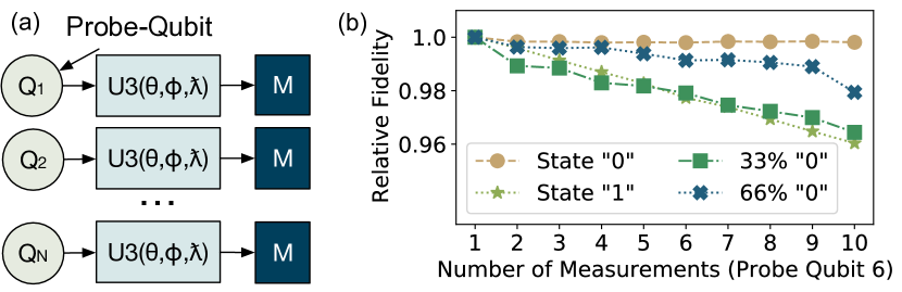
To study measurement crosstalk, we perform several characterization experiments on IBMQ hardware. Figure 2(a) shows an N-qubit circuit that creates arbitrary quantum states using single-qubit U3 gates (Abhijith et al., 2018). During the experiment, the Probe-Qubit (Q1) is always mapped to the physical qubit on which the impact of measurement crosstalk is being determined, whereas the other N-1 qubits are randomly mapped to the remaining physical qubits of the machine in each sample and generate multiple samples for each N. Note that N denotes the number of measurements and N=1 corresponds to the case when the Probe-Qubit is measured in isolation. For the results shown in Figure 2(b), we vary N from 1 to 10 and take 10 samples for each N.
We compute the mean fidelity of the Probe-Qubit for each N by measuring the Total Variation Distance (TVD) between the experimental output and the output from a noise-free quantum computer. Figure 2(b) shows the impact of increasing the number of measurements from 1 to 10 for four different quantum states, prepared by specifying the Euler angles for the U3 gates, when Qubit-6 is probed on 27-qubit IBMQ-Paris. We observe that simultaneously measuring a larger number of qubits can reduce the fidelity of these operations significantly. We make similar observations on other qubits and hardware devices. Further experiments also show that the impact of such crosstalk depends on the quantum state and physical qubit and therefore, is hard to characterize. Prior studies state that it is hard to fully understand and minimize measurement crosstalk at device level (Khezri et al., 2015; Arute et al., 2019).
3.2. Impact of Spatial Variation
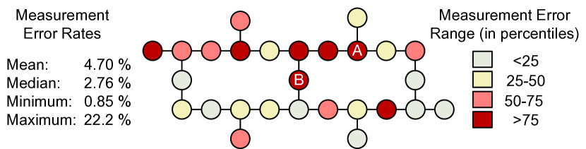
To execute a program on a NISQ device, a compiler maps the program qubits onto the physical qubits of the device and translates the high-level program into low-level machine specific instructions. Compilers also need to insert SWAP instructions to overcome the limited connectivity of NISQ devices. Noise-aware compilers (Murali et al., 2019a; Tannu and Qureshi, 2019c) account for the error characteristics of the underlying quantum hardware and avoid mapping program qubits on to hardware qubits with worst-case errors. However, while this works very efficiently for small programs, spatial variation in measurement error rates often force compilers to map program qubits on unreliable physical qubits, as programs grow in size, because the qubits with the lowest error rates are not spatial neighbors, as shown in Figure 3. For example, it is not possible to map any program with more than six qubits on the 27-qubit IBMQ-Toronto without using a physical qubit with more than 2.7% measurement error-rate (the median error-rate). Further, the compiler is forced to use physical qubits A and B with more than 20% measurement error rate for programs with sixteen and twenty-one qubits or more respectively.
3.3. The Insight: Measurement Subsetting
NISQ applications measure all the program qubits in each trial, subjecting all the trials to the accumulated measurement errors from all the qubits. We can reduce the impact of measurement errors on the fidelity of NISQ programs by:
-
(1)
Reducing the number of measurement operations by performing some trials with measurements only on a subset of qubits and effectively lowering the impact of crosstalk.
-
(2)
Remapping to ensure that the subset measurements are performed on the qubits with the lowest error rates. This allows the us to get an effective measurement error rate that is closer to the minimum rather than the average.
Correlation versus Fidelity Trade-off in Subsetting:
Quantum computers obtain their exponential power by creating and manipulating highly correlated states. To measure this correlated state, a NISQ program measures all the qubits in each trial. If there was no correlation, and each qubit had an independent probability of being in the or state, then one could simply split the trials into N groups (one group for each qubit), obtain the independent probability of being in or state for each qubit, and then obtain the probability distribution over all the qubits through multiplication. While this approach has high fidelity for each trial (only one measurement), it captures zero correlation between the qubits. Measuring a subset of qubits (larger than a single qubit but not all qubits) captures some correlation (within the measured qubits) but the correlations between these marginal distributions remain unknown, and therefore, multiplication or a tensor product may not yield the correct output distribution.
3.4. The Goal: Reducing Measurement Errors
Thus, measuring all the qubits provides full correlation (but low fidelity) and fewer measurements provide higher fidelity (but weaker correlation). Ideally, we want both full correlation and high fidelity. The goal of this paper is to design scalable and effective policies that can improve application fidelity by retaining the global correlation of the original program, while simultaneously benefiting from the higher fidelity obtained from fewer measurements. Next, we discuss our proposed design, JigSaw.
4. JigSaw: Overview and Design
We propose JigSaw, a framework that relieves the NISQ program from requiring to measure all the qubits of a program in each trial. Figure 4 shows the overview of JigSaw. JigSaw executes a program in two modes. First, JigSaw executes half of the trials in the global-mode in which a program is executed in its entirety and all the qubits are measured to obtain the global probability mass function (PMF).222We use Probability Mass Function (PMF) for the results of program execution because these include discrete and not continuous values. Second, for the remaining trials, JigSaw runs additional copies of the program or Circuits with Partial Measurements (CPM) that measure fewer qubits in the subset-mode, to obtain more accurate marginal or local-PMFs over the subset of qubits being measured. However, CPM alone cannot be used to infer the output PMF of a program without information about the correlations between these local-PMFs. To address this challenge, JigSaw employs a post-processing or reconstruction step that updates the global-PMF using the local-PMFs. This enables JigSaw to improve the application fidelity while simultaneously retaining the global correlation without requiring any additional trials.
4.1. Global-Mode: Generation of Global-PMF
In this mode, JigSaw executes the entire program and measures all the program qubits to produce a global-PMF. This is identical to the baseline policy and is done for half of the trials. We use Noise-Aware SABRE (Li et al., 2018) for compilation to obtain a global-PMF with high fidelity. A NISQ compiler maps the logical qubits of a program on to the physical qubits of the hardware and generates a schedule by translating the high-level instructions into low-level machine specific operations. To overcome limited connectivity on NISQ hardware, compilers also insert SWAP instructions to bring two non-adjacent qubits next to each other, so that CNOT operations can be performed between them. Noise-Aware SABRE accounts for the hardware error characteristics and generates a schedule that maximizes the Expected Probability of Success (EPS) (Nishio et al., 2019). EPS is the expected probability of successfully executing each gate and measurement operation in a schedule and is computed at compilation time by using the error rates obtained from the daily calibration report of the NISQ hardware.
4.2. Subset-Mode: Generation of Local-PMFs
In the subset-mode, JigSaw runs several Circuits with Partial Measurements (CPM), for the remaining half of the trials which are equally distributed between the CPM. We discuss how CPM are generated and optimized for greater fidelity.
4.2.1. Circuits with Partial Measurements
A CPM is identical to the original program, except that it measures only a subset of qubits. CPM produces high-fidelity local-PMFs over the qubits measured. For example, Figure 5(a) shows a CPM of a BV-4 program that measures 2 qubits, and . The key parameter in JigSaw is the number of qubits measured in a CPM and is called the subset size. Our default design uses CPM that measure 2 qubits. This is the smallest possible subset size that captures some correlation while performing fewest possible measurements. Measuring only one qubit in a CPM captures zero correlation and therefore, not used. By default, we use a sliding window method to generate the CPM so that we get N unique CPM for an N-qubit program. For example, for a -qubit program with qubits , we generate CPM, measuring , and . Therefore, the number of CPM is same as the number of qubits.

4.2.2. Optimizations to Improve Fidelity of the CPM
As JigSaw heavily relies on the accuracy of the local-PMFs, the compiler recompiles each CPM to maximize their fidelity.
Optimizing for Measurement Errors: We recompile each CPM to exploit variability in measurement errors and ensure that measurements of desired program qubits are performed on the strongest physical qubits. The compiler avoids measurements on the physical qubit(s) with the highest readout error rate, referred to as vulnerable qubit(s), in an allocation. For example, the compiler eliminates the allocation in Figure 5(b) for the CPM in Figure 5(a) to avoid readout of on the vulnerable qubit and selects an alternate allocation.
Avoiding Extra SWAPs: To avoid measurement on the vulnerable qubit(s), the compiler often uses alternate qubit allocations, some of which may need insertion of extra SWAP instructions. However, we avoid such allocations that require extra SWAPs to avoid additional gate errors. For example, the compiler selects the allocation shown in Figure 5(d) over Figure 5(c) because the latter requires an extra SWAP (SWAP , ). While in most cases, the compiler finds alternate mappings without incurring extra SWAPs, for cases where the compiler cannot not find a mapping without inserting an extra SWAP, it picks the mapping that maximizes the EPS.
The ability to find alternative mappings depends on device connectivity, spatial location of good qubits, and program characteristics. Our studies show most CPM can reuse qubit allocations chosen by the Ensemble of Diverse Mappings (Tannu and Qureshi, 2019a) policy. Also, we use SABRE, which has low latency.
4.3. Post-processing via Bayesian Method
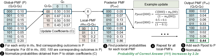
JigSaw produces (N+1) PMFs for a program with N qubits: one global-PMF and one local-PMF for each of the N CPMs. The post-processing step aims to combine the higher fidelity local-PMFs from each CPM into the global-PMF. To this end, we propose Bayesian Reconstruction algorithm, which is inspired by Bayesian updating in statistics, whereby a prior probability estimate is updated using additional information (Joyce, 2003). For JigSaw, the global-PMF (P) offers the prior probability estimate, whereas the set of marginals (M) obtained from the CPM provides the additional information. We use the term marginal to denote a set comprising of a subset of qubits measured in a CPM and the local-PMF produced by the CPM.
Consider an example of a 3-qubit program. Let represent a generic global-PMF of a -qubit program (with qubits ), where a to h are the probabilities of observing outcomes to respectively. Similarly, refers to a generic marginal for a CPM measuring qubits .
The steps for the Bayesian Reconstruction algorithm are described in Algorithm 1 (Appendix). The algorithm uses each marginal to update the probabilities of each outcome in the global-PMF (P). The algorithm starts by searching for all outcomes in P associated with each outcome in a marginal, by evaluating the bits at the corresponding qubit positions. For example, for in the marginal , the candidates in P are and . For each marginal in M, the Bayesian Update function generates an updated PMF () by updating the probabilities of each outcome in P using the associated probabilities in the marginals. For example, the probabilities of and , i.e., a and d respectively, are updated in proportion with (corresponding to in m0). The algorithm produces a posterior output PMF () by adding all the intermediate PMFs () to the global-PMF (). The algorithm is recursively called and terminates when the Hellinger Distance (Hellinger, 1909) between the output PMF, , prior to and post the function call does not change, implying the two PMFs are similar.
We explain the steps involved in the Bayesian update using a quantitative example. Figure 6 shows the update sequence using experimental data for a 3-qubit program whose global-PMF is denoted by in order using a marginal from a CPM that measures .
-
•
Step 1 : The algorithm searches for all candidate outcomes in for each entry in marginal by evaluating the bits at the corresponding qubit positions. For example, and are the candidate outcomes in for in , obtained by matching the values for in and .
-
•
Step 2 : Next, the function computes the Update Coefficients for each of the outcomes in by normalizing their respective probabilities of occurrence in .
-
•
Step 3 : Next, the algorithm computes the posterior probabilities for each observed outcome in by scaling them using the corresponding probabilities observed in . Figure 6 explicitly shows the computation for obtaining the posterior probability of outcome () using the Update Coefficient and marginal information .
-
•
Step 4 : The algorithm repeats Steps 1-3 to generate an intermediate posterior PMF () for each marginal.
-
•
Step 5 : Each is added to the global-PMF ().
-
•
Step 6 : The final output PMF () is obtained by normalizing the probabilities.
For readability, Figure 6 only shows the steps for marginal [], whereas the output PMF shown is obtained from recursive updates with additional marginals. Note that as the Bayesian updates for each CPM are performed independently and the intermediate PMFs are added in the final step, the order of updates does not matter.
4.4. Multi-Layer JigSaw (JigSaw-M)
Our studies show that the performance of JigSaw saturates when additional CPM of the same subset size that do not offer any incremental information are used. However, we can design more unique CPM by using different subset sizes and improve the application fidelity even further.
4.4.1. Global and Subset-Modes for JigSaw-M
The global mode for JigSaw-M is identical to JigSaw that generates the global-PMF by executing the program and measuring all the qubits. The subset-mode for JigSaw-M executes CPM of non-uniform subset sizes s, such that , where and are the maximum and minimum subset sizes respectively. We use a sliding window method to generate unique CPM for each subset size, similar to JigSaw, but other methods can be used too. If CPM of different sizes are used, JigSaw-M produces (N+1) PMFs for an N-qubit program, one global-PMF and N local-PMFs for each subset size. By default, our design uses CPM of sizes 2 to 5.
4.4.2. Adapting Reconstruction for JigSaw-M
JigSaw-M comprises of CPM of different sizes. There is a choice between which CPM must be used first to update the global-PMF. However, note that there exists a trade-off between the fidelity of a CPM and the correlation it can capture depending on the number of qubits measured in the CPM. A smaller CPM offers higher fidelity due to fewer measurement errors but captures limited correlation. Alternately, a larger CPM offers higher correlation, but has lower fidelity since it is more prone to measurement errors. Thus, for JigSaw-M, the reconstruction algorithm first updates the global-PMF using the CPM of the highest size (), limiting the loss of global correlation. The updated PMF () is then further enhanced using information from CPM of the next higher size. The process is repeated until the smallest CPM are used. This top-down ordering maximally preserves the global correlation, while simultaneously improving the fidelity.
We discuss the evaluation methodology before discussing the impact of JigSaw on the fidelity of NISQ applications.
5. Evaluation Methodology
5.1. Quantum Hardware Platforms
For all our evaluations, we use three different quantum computers from IBM: -qubit IBMQ-Toronto, -qubit IBMQ-Paris, and -qubit IBMQ-Manhattan.
5.2. Baseline Compiler
For the baseline, we use Noise-Aware SABRE (Li et al., 2018) to compile and map the program onto the physical qubits with the lowest error rates. We also evaluate JigSaw against an Ensemble of Diverse Mappings (EDM) policy that runs independent copies of the program on different groups of physical qubits (Tannu and Qureshi, 2019a) and improves the ability to infer the correct answer. Note that while we use Noise-Aware SABRE, other noise-adaptive compilers (Murali et al., 2019a; Tannu and Qureshi, 2019c) may be used too.
5.3. Benchmarks
We use the benchmarks described in Table 2. The type and size of benchmarks are derived from prior works (Li et al., 2018; Tannu and Qureshi, 2019c; Murali et al., 2019a; Tannu and Qureshi, 2019a). Note that the IBMQ machines used for evaluations have a Quantum Volume (Cross et al., 2019) of 32, which means that square circuits of only up to size 5 can be run reliably and therefore, the size of the benchmarks used is already much larger even if they do not use all the qubits that are present on the machine.
| Name | Algorithm | #Qubits | 1Q | 2Q |
| (n) | Gates | Gates | ||
| BV-n | Bernstein-Vazirani (Bernstein and Vazirani, 1997) | 6 | 2(n+1) | n |
| Graycode-n | Graycode Decoder | 18 | n/2 | (n-1) |
| QAOA-n (p=1) | Maxcut with p=1 (Farhi et al., 2014) | 8 | 4n | (n-1) |
| QAOA-n (p=2) | Maxcut with p=2 | 10, 14 | 6n | 2(n-1) |
| QAOA-n (p=4) | Maxcut with p=4 | 10, 12 | 10n | 4(n-1) |
| GHZ-n | Greenberger-Horne | 14 | 1 | (n-1) |
| -Zeilinger (Greenberger et al., 1989) | ||||
| Ising-n | Ising model (Ising, 1925) | 10 | n(4.5n-2) | n(n-1) |
5.4. Experimental Setup: Number of Trials
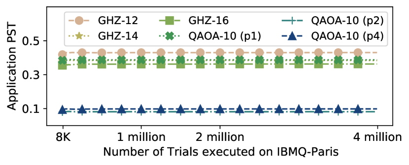
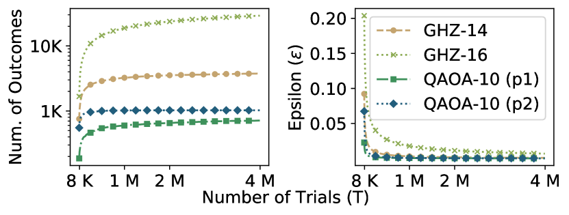
We use between 32K to 256K trials for the baseline depending on program size. This represents the highest fidelity that can be obtained by increasing trials alone and serves as a strong baseline as more trials do not improve fidelity (mainly due to correlated errors). Figure 7 shows the Probability of Successful Trial (PST) of several GHZ and QAOA benchmarks executed on IBMQ-Paris for up to 4 million trials. We observe similar behavior for other workloads and machines.
For EDM (Tannu and Qureshi, 2019a), we use an ensemble of four mappings and the trials are equally divided among the mappings. For JigSaw and JigSaw-M, the trials are equally split between the global-mode and the subset-mode. In the subset-mode the trials are equally split between all the CPM for both JigSaw and JigSaw-M. Therefore, JigSaw, JigSaw-M, and EDM all use the same number of trials as the baseline. We run all the experiments within the same calibration cycle but observe similar results across different calibration cycles. We use equal split for simplicity because the fidelity saturates for the number of trials used in our evaluation. If the number of trials is severely limited, the split between global-mode and subset-mode can be tuned to possibly obtain even larger gains. We provide an estimate of the number of trials required for each CPM in Appendix A.2.
5.5. Figure-of-Merit
At present, there is no standard single metric to evaluate NISQ application fidelity. Therefore, for our evaluations, we study three generic metrics and an application-specific figure-of-merit for the QAOA benchmarks. These metrics are derived from prior works and the details are discussed below:
(1) Probability of Successful Trial (PST) (Tannu and Qureshi, 2018, 2019c, 2019a; Liu and Zhou, [n. d.]; Das et al., 2019; Murali et al., 2019a) is the ratio of the number of trials with the correct output to the total number of trials, as described in Equation (1).
| (1) |
(2) Inference Strength (IST) (Tannu and Qureshi, 2019a; Liu and Zhou, [n. d.]; Patel and Tiwari, 2020b) is used to quantify the ability to infer the solution and distinguish it from incorrect outcomes. IST is defined as the ratio of the probability of occurrence of the correct outcome to the probability of occurrence of the most frequent erroneous outcome, as shown in Equation (2).
| (2) |
(3) Fidelity of a program is obtained by measuring the Total Variation Distance (TVD) (Wikipedia, 2020) between the output distributions on a noise-free quantum computer (P) and real hardware (Q). TVD allows us to measure the fidelity of quantum programs (Sanders et al., 2015) whose output can be a probability distribution with more than one correct answer. The Fidelity ranges between 0 and 1, where 1 represents two identical distributions and 0 means completely dissimilar distributions, as shown in Equation (3). While we use TVD, Hellinger Distance (Hellinger, 1909; Das et al., 2019) or Kullback–Leibler divergence (Kullback, 1997) may be used too and these metrics are closely related (Wikipedia, 2020).
| (3) |
A higher Probability of Successful Trial (PST), Fidelity, and Inference Strength (IST) is desirable.
(4) Approximation Ratio Gap (ARG) (ala, 2020) is an application-specific metric for Quantum Approximate Optimization Algorithm (QAOA) (Farhi et al., 2014) benchmarks. To solve MaxCut problems with QAOA, the classical cost function which must be maximized is translated into a cost Hamiltonian and the goal is to maximize the expectation value of the cost Hamiltonian. The expectation value of a cost function is computed by taking a mean over the samples in the output distribution of the QAOA circuit. The Approximation Ratio (AR) is defined as the ratio between the mean cost function value over these samples and the actual maximum function value of the optimal solution and is used to quantify QAOA performance (Crooks, 2018; Zhou et al., 2020). The Approximation Ratio Gap (ARG) denotes the percentage difference between the approximation ratio obtained on an ideal quantum computer (AR) and real hardware (AR), as described in Equation (4). A lower ARG is desired as it indicates a performance closer to the noise-free scenario.
| (4) |
6. Results and Sensitivity Studies
In this Section, we discuss the impact of JigSaw on the reliability of NISQ applications.
6.1. Results for Probability of Successful Trial
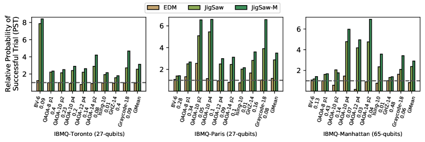
Figure 8 shows the improvement in Probability of Successful Trial (PST) using JigSaw and JigSaw-M. Our evaluations using three different quantum hardware from IBM and tens of quantum benchmarks show that JigSaw the PST by 2.91x on average and by up-to 7.87x compared to the baseline. JigSaw-M improves PST by 3.65x on average and up-to 8.42x compared to the baseline. Compared to JigSaw, JigSaw-M improves the PST of applications by 1.26x on average and up-to 1.72x.
6.2. Results for Inference Strength
Inference Strength (IST) determines the capability to suppress correlated errors and infer the correct answer of a program from the the output PMF. Table 3 shows the improvement in IST for EDM, JigSaw, and JigSaw-M relative to the baseline. Note that the average here is the geometric mean. JigSaw improves the IST on average by 2.19x and up-to 21.7x compared to the baseline, whereas JigSaw-M improves the IST on average by 2.82x and up-to 27.9x. Unlike EDM which only improves the IST, JigSaw improves both PST and IST.
| IBMQ | EDM | JigSaw | JigSaw-M | ||||||
|---|---|---|---|---|---|---|---|---|---|
| (Hardware) | Min | Max | Avg | Min | Max | Avg | Min | Max | Avg |
| Toronto | 0.92 | 2.25 | 1.36 | 1.22 | 21.7 | 2.87 | 1.23 | 27.9 | 3.84 |
| Paris | 0.78 | 6.54 | 1.36 | 1.07 | 9.07 | 2.33 | 1.09 | 28.1 | 3.13 |
| Manhattan | 0.75 | 2.74 | 1.27 | 0.81 | 3.12 | 1.35 | 0.83 | 3.40 | 1.46 |
6.3. Results for Fidelity
Table 4 compares the Fidelity for EDM, JigSaw, and JigSaw-M relative to the baseline. For instance, on IBMQ-Toronto, EDM degrades Fidelity by 0.96x on an average, whereas JigSaw and JigSaw-M improve it by 2.17x and 2.54x respectively. Overall, JigSaw improves the Fidelity on average by 2.12x, whereas JigSaw-M improves the Fidelity on average by 2.47x and by up-to 8.41x compared to the baseline. Therefore, the output distributions of programs obtained from JigSaw and JigSaw-M have higher Fidelity and are significantly more similar to the distributions obtained on a noise-free quantum computer.
| IBMQ | EDM | JigSaw | JigSaw-M | ||||||
|---|---|---|---|---|---|---|---|---|---|
| (Hardware) | Min | Max | Avg | Min | Max | Avg | Min | Max | Avg |
| Toronto | 0.78 | 1.22 | 0.96 | 1.07 | 7.86 | 2.17 | 1.07 | 8.41 | 2.54 |
| Paris | 0.77 | 2.54 | 1.19 | 1.09 | 5.07 | 2.33 | 1.11 | 6.52 | 2.77 |
| Manhattan | 0.43 | 1.62 | 0.93 | 1.18 | 3.26 | 1.84 | 1.28 | 4.43 | 2.10 |
6.4. Results for Approximation Ratio Gap
We use Approximation Ratio Gap (ARG) as an application-specific metric for the QAOA benchmarks. A lower ARG is desired as it indicates a performance closer to the noise-free scenario (ala, 2020). Table 5 compares the ARG for the QAOA benchmarks evaluated in this paper. We observe that JigSaw reduces the ARG by 0.41x on average and by up-to 0.14x compared to the baseline. Alternately, JigSaw-M reduces the ARG by 0.31x on average and up-to 0.08x compared to the baseline. Overall, JigSaw and JigSaw-M consistently outperforms the baseline and EDM. Overall, JigSaw outperforms the baseline and prior work, EDM (Tannu and Qureshi, 2019a), across all the four metrics.
| Machine | Workload | Baseline | EDM | JigSaw | JigSaw-M |
|---|---|---|---|---|---|
| Tor | QAOA-8 p1 | 19.6 | 19.4 | 2.83 | 1.59 |
| QAOA-10 p2 | 24.5 | 24.0 | 12.3 | 10.6 | |
| QAOA-10 p4 | 23.4 | 24.3 | 10.5 | 8.50 | |
| QAOA-12 p4 | 12.3 | 13.8 | 4.82 | 3.11 | |
| QAOA-14 p2 | 9.86 | 9.74 | 4.06 | 2.48 | |
| Par | QAOA-8 p1 | 21.7 | 17.5 | 3.91 | 2.50 |
| QAOA-10 p2 | 35.0 | 29.2 | 19.0 | 16.3 | |
| QAOA-10 p4 | 30.3 | 29.4 | 8.60 | 6.19 | |
| QAOA-12 p4 | 10.5 | 11.8 | 5.63 | 4.98 | |
| QAOA-14 p2 | 8.50 | 9.66 | 3.95 | 2.95 | |
| Man | QAOA-8 p1 | 18.2 | 18.4 | 8.87 | 8.23 |
| QAOA-10 p2 | 28.1 | 31.9 | 19.3 | 19.8 | |
| QAOA-10 p4 | 31.1 | 29.9 | 13.7 | 11.1 | |
| QAOA-12 p4 | 14.1 | 26.6 | 5.12 | 2.94 | |
| QAOA-14 p2 | 11.5 | 14.3 | 5.93 | 4.49 |
6.5. Impact of Number of Circuits with Partial Measurements and Selection Method
Our default design uses a sliding window method to generate a handle of unique CPM. To understand the impact of the number of CPM and selection method, we perform an empirical study using a -qubit QAOA program on IBMQ-Paris.
Sensitivity to Number of CPM: The total number of possible CPM (measuring two qubits) for a Q qubit program is . To understand the impact of the number of CPM on its effectiveness, JigSaw randomly generates circuits with partial measurements of subset size out of all the 66 possibilities ( = 66) and uses these local-PMFs to update the global-PMF. The process is repeated hundreds of times for each and Figure 9(a) shows the average improvement in Application PST from JigSaw as is increased.
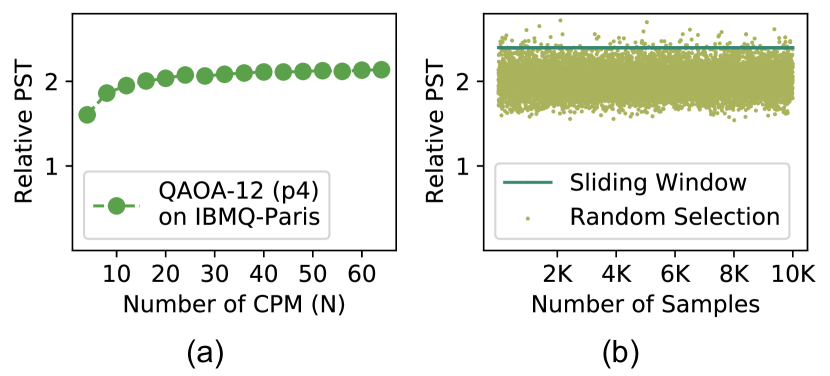
We observe that the performance of JigSaw saturates when additional CPM do not offer incremental information. Thus, only a few and unique CPM are sufficient for JigSaw to be effective. Further, to obtain a greater number of unique CPM, JigSaw-M generates CPM of non-uniform subset sizes.
Sensitivity to CPM Selection Method: To study the impact of CPM selection method, JigSaw randomly selects a group of CPM of subset size 2 from all the 66 possibilities while ensuring that each program qubit is measured in a CPM at least once. As there are 12 qubits in the program JigSaw selects 12 random CPM each time and the process is repeated 10,000 times. Figure 9(b) shows the relative improvement in PST for this study, and we observe that we get similar results irrespective of the CPM. Thus, although our default design uses a sliding window method, JigSaw is equally effective even if any other technique to generate the CPM is used.
6.6. Impact of Recompilation
JigSaw mainly benefits from measurement subsetting and recompilation. By recompiling each CPM, the effective measurement error-rates for CPM are close to the best-case qubits rather than close to the average-case qubits (which is the case for the global-mode and the baseline). For example, Figure 10 shows that the probability of correctly measuring a qubit in a CPM increases by up-to 3.25x compared to the baseline for a BV-6 benchmark on IBMQ-Toronto. Note that the probability of correctly measuring a qubit is computed from the set of outcomes where the particular qubit is correctly measured, even if the overall outcome is erroneous and does not represent the correct answer. Thus, recompiling CPM can significantly enhance the effectiveness of JigSaw.
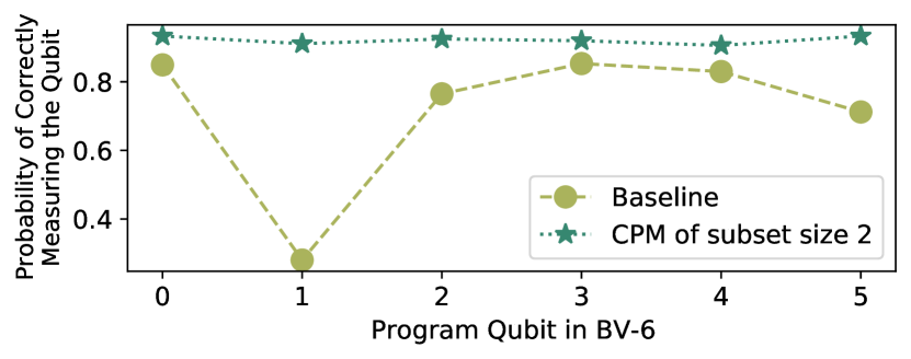
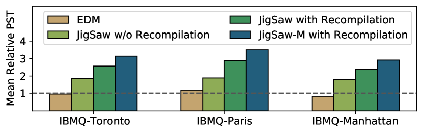
Figure 11 shows the Mean PST from JigSaw without recompilation (subsetting only), JigSaw with recompilation, and JigSaw-M relative to the baseline. Without recompilation, JigSaw improves the PST by 1.92x on average and up-to 3.26x, whereas with recompilation JigSaw improves the PST by 2.91x on average and up-to 7.8x compared to the baseline. With recompilation, JigSaw-M improves the PST by 3.65x on average and by up-to 8.4x.
7. Scalability of Reconstruction
The applicability of reconstruction algorithms is often limited by their memory and time complexity. For example, tensor-product based algorithms are extremely hard to scale due to their exponential complexity. Therefore, we study the scalability of our proposed Bayesian Reconstruction using an analytical model, described next.
7.1. Insight: Bounded by Observations
JigSaw limits the complexity of the reconstruction algorithm by storing and updating only the non-zero entries generated in the global-mode. Although the number of possible non-zero entries in the global-PMF can scale exponentially with the program size, the actual number of entries observed is much lower and is limited by the number of trials, particularly for large programs. For example, there are possible outcomes for a -qubit program, and assuming the circuit produces a uniform distribution, it would require a minimum of or trials to observe each of these outcomes at least once, which is impractical. In practice, we may be able to execute at-most a few million trials, since the time to execute the trials still increases linearly with the number of trials. Moreover, practical quantum algorithms are designed to produce output distributions with relatively low variance and bounded possible outcomes. For example, Table 6 shows that a Graycode-18 benchmark produces only up to K unique outcomes when executed for K trials, even though K (=) outcomes are possible. We bound the complexity of JigSaw reconstruction by focusing only on the outcomes observed rather than all the possible outcomes.
| Outcomes | IBMQ-Toronto | IBMQ-Paris | IBMQ-Manhattan |
|---|---|---|---|
| Observed (Obs) | 17.0 K | 17.3 K | 18.5 K |
| Maximum (Max) | 256 K | 256 K | 256 K |
| Ratio (Obs/Max) | 6.6 % | 6.8 % | 7.2 % |
7.2. Memory Complexity
JigSaw only stores non-zero entries in the global, output, local PMFs, and an intermediate PMF for each CPM. We assume is the number of CPM. For simplicity, we assume the global-mode and each CPM in subset-mode uses trials.333For simplicity, we assume up-to 1 million trials each for the global-mode and each CPM, which is a severely pessimistic assumption. In practice, the trials are split between a large number of CPM, so the storage and timing complexity gets reduced further.
Global, Intermediate, and Output PMFs: Each global-PMF entry comprises of an n-bit string outcome and its probability of occurrence, as shown in Figure 12(a). We assume entries in the global-PMF, where . As JigSaw only updates the probabilities of the global-PMF entries, the intermediate and output PMFs are only required to store the updated probabilities, as shown in Figure 12(b). Hence, the global-PMF requires () bytes per entry, whereas the intermediate and output PMFs each require bytes per entry.

Our experiments on IBMQ systems show that and does not change rapidly with increasing trials. For example, Figure 13 shows the number of unique outcomes and when some GHZ and QAOA benchmarks are executed for trials on IBMQ-Paris.
Local-PMFs: A local-PMF for a CPM of subset size consists of entries, where , and requires bytes, as shown in Figure 12(c). To minimize errors on CPM, s must be small such as in the default JigSaw design. For such small , a local-PMF consists of all possible entries. But for large , and is denoted by . For example, local-PMFs of size and for a GHZ-14 program on IBMQ-Toronto contain and entries respectively, even though entries are possible for .
JigSaw stores one Global-PMF, intermediate PMFs, one output PMF and local-PMFs. JigSaw-M stores one Global-PMF, intermediate PMFs, one output PMF and local-PMFs where subset sizes are used. Although JigSaw-M uses more CPM, since it employs hierarchical reconstruction from the highest to the lowest subset size, only intermediate PMFs are required which are reused across reconstruction rounds. Thus, the total memory capacity (in bytes) is given by Equation (5). The memory complexity for JigSaw is obtained for since it uses CPM of a single subset size only.
| (5) |
7.3. Time Complexity
JigSaw updates each Global-PMF entry for each entry in a local-PMF. Obtaining the update coefficients require operations and the update itself requires operations per local-PMF. Assuming JigSaw uses CPM, it requires operations. Similarly, JigSaw-M requires operations. As JigSaw only stores and updates non-zero PMF entries, which is much lower than the maximum possible, and is limited by the number of trials, the time-complexity increases linearly with the number of trials and qubits.
7.4. Results for Scalability Analysis
Table 7 shows the memory and number of operations required for programs of different input sizes , values of , , and number of trials . To obtain the typical complexity, we use and (from Figure 13), whereas we use to obtain the upper bound. For JigSaw, we assume CPM of subset size 5 and the number of CPM () to be same as the number of qubits in the program (as our default design). For JigSaw-M, we assume sizes 5,10,15, and 20. We observe that the storage and time complexity is linear with the number of trials and qubits in the program, making JigSaw applicable to programs with hundreds of qubits.
| Qubits | Trials | JigSaw | JigSaw-M | |||
| (n) | () | Mem | OPs | Mem | OPs | |
| 100 | 0.05 | 32K | 0.01 | 0.66 | 0.02 | 2.64 |
| 1024K | 0.05 | 21.0 | 0.42 | 83.9 | ||
| 1.0 | 32K | 0.03 | 13.1 | 0.20 | 52.4 | |
| 1024K | 0.96 | 419 | 3.97 | 1677 | ||
| 500 | 0.05 | 32K | 0.01 | 3.28 | 0.1 | 13.12 |
| 1024K | 0.24 | 105 | 2.09 | 419 | ||
| 1.0 | 32K | 0.15 | 65.5 | 0.99 | 262 | |
| 1024K | 4.74 | 2097 | 19.8 | 8388 | ||
8. Related Work
Software mitigation of NISQ hardware errors (Gokhale et al., 2019, 2020; Zulehner et al., 2018; Murali et al., 2019a; Nishio et al., 2019; Shi et al., 2019; Tannu and Qureshi, 2019a, 2018; Wilson et al., 2020; Das et al., 2019; Huang and Martonosi, 2019; Murali et al., 2020a, 2019b; of Sciences Engineering and Medicine, 2019; Shi et al., 2020; Patel et al., 2020; Patel and Tiwari, 2021) is an active area of research. More recently, schemes that specifically reduce the impact of measurement errors have been proposed (IBM, 2010; Bravyi et al., 2020; Kwon and Bae, 2020; Tannu and Qureshi, 2019b; Barron and Wood, 2020; Patel and Tiwari, 2020a). We compare with two of these proposals, and then other works.
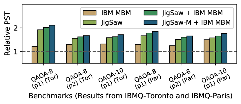
Matrix-Based Error Mitigation: IBM’s matrix-based complete measurement error mitigation (MBM) post-processes the outputs of an n-qubit program using a x inverse noise matrix prepared by calibrating basis states (IBM, 2010). Jigsaw can be combined with MBM for even higher fidelity than either scheme standalone, as shown in Figure 14. Note that the complexity of MEM grows exponentially with the program size, whereas JigSaw needs no characterization and its post-processing step has linear complexity.
State-Based Error Mitigation: Few prior schemes transform a more error-prone quantum state to a less susceptible one (Kwon and Bae, 2020; Tannu and Qureshi, 2019b) using single qubit gates, but has limited applicability on recent devices as they do not exhibit considerable bias in measuring state “1” over state “0”. For example, the average probabilities of incorrectly measuring states “0” and “1” on IBMQ-Manhattan are 2.3% and 3.6%, respectively. We make similar observations on other machines too.
Related Works in Circuit Decomposition: Peng et. al. (Peng et al., 2019) proposed circuit decomposition techniques and discussed the mathematical validity of executing a larger program on smaller quantum machines. A scalable approach for efficient circuit cutting was introduced in (Tang et al., 2020). However, these approaches use tensor products and are hard to scale. On the contrary, JigSaw utilizes circuits identical to the original program except the reduced measurements and incurs linear complexity, making it scalable and applicable to all programs. Shehab et. al. (Shehab et al., 2019) use partial circuits to reduce computations and improve fidelity for QAOA applications.
9. Conclusion
In this paper, we propose JigSaw- a design that mitigates the impact of measurement errors by executing programs in two modes: global-mode in which the program measuring all the qubits generates a global Probability Mass Function (PMF) over all the qubits, and subset-mode in which multiple Circuits with Partial Measurements (CPM) produce local-PMFs over only the measured qubits. The global-PMF offers full correlation but low fidelity, whereas the local-PMFs offer higher fidelity but poor correlation. By employing Bayesian updates and the local-PMFs, JigSaw enhances the global-PMF and improves the success rate of applications on average by 2.91x and up-to 7.87x. We also propose Multi-Layer JigSaw (JigSaw-M) which uses a larger number of unique CPM of non-uniform subset sizes and employs an ordered reconstruction algorithm to enhance the global-PMF. Overall, JigSaw-M improves the success rate of applications on average by 3.65x and up-to 8.42x.
Acknowledgements.
We thank Nicolas Delfosse for helpful discussions and feedback. We also thank Sanjay Kariyappa, Ananda Samajdar, and Keval Kamdar for editorial suggestions. Poulami Das was funded by the Microsoft Research PhD Fellowship. This research used resources of the Oak Ridge Leadership Computing Facility at the Oak Ridge National Laboratory, which is supported by the Office of Science of the U.S. Department of Energy under Contract No. DE-AC05-00OR22725.Appendix A APPENDIX
A.1. Bayesian Reconstruction
The Bayesian Reconstruction algorithm is shown in Algorithm 1.
A.2. Estimate for the Number of Trials
For simplicity, by default we execute the global-mode for half of the trials and the subset-mode for the remaining half. We also equally distribute the trials in the subset-mode between the CPM for both JigSaw and JigSaw-M. However, if the trials are severely limited, (1) the distribution of trials may be fine-tuned or (2) the subset-mode may be executed for few thousands of extra trials (global-mode corresponds to the baseline). We perform an analysis of how the trials may be allocated for each CPM.
Let there be possible outcomes for a program that measures qubits. If is the probability of observing an outcome and each of the outcomes is equally likely to appear at the end of a trial, then . The probability that a given outcome has appeared at least once after trials is then given by Equation (6).
| (6) |
If and is large, may be approximated as Equation (7).
| (7) |
Thus, in order to obtain the given outcome at least once with probability , the number of trials required is given by Equation (8).
| (8) |
Hence, the total number of trials required to observe every possible outcome at least once with probability is given by Equation (9).
| (9) |
We measure only 2 qubits in each CPM in the default JigSaw design and thus, only about 150 trials are required to ensure (with 99.99% probability) that we obtain each possible answer at-least one time. Similarly, as JigSaw-M uses CPM of different sizes, the estimated number of trials would still range within a few thousands.
References
- (1)
- ala (2020) 2020. Circuit Compilation Methodologies for Quantum Approximate Optimization Algorithm, author=Alam, Mahabubul and Ash-Saki, Abdullah and Ghosh, Swaroop. In 2020 53rd Annual IEEE/ACM International Symposium on Microarchitecture (MICRO). IEEE, 215–228.
- Abhijith et al. (2018) J Abhijith, Adetokunbo Adedoyin, John Ambrosiano, Petr Anisimov, Andreas Bärtschi, William Casper, Gopinath Chennupati, Carleton Coffrin, Hristo Djidjev, David Gunter, et al. 2018. Quantum algorithm implementations for beginners. arXiv e-prints (2018), arXiv–1804.
- AI (2021) Google Quantum AI. 2021. Exponential suppression of bit or phase errors with cyclic error correction. Nature 595, 7867 (2021), 383.
- Arute et al. (2019) Frank Arute, Kunal Arya, Ryan Babbush, Dave Bacon, Joseph C Bardin, Rami Barends, Rupak Biswas, Sergio Boixo, Fernando GSL Brandao, David A Buell, et al. 2019. Supplementary information for” Quantum supremacy using a programmable superconducting processor”. arXiv preprint arXiv:1910.11333 (2019).
- Barron and Wood (2020) George S Barron and Christopher J Wood. 2020. Measurement error mitigation for variational quantum algorithms. arXiv preprint arXiv:2010.08520 (2020).
- Bernstein and Vazirani (1997) Ethan Bernstein and Umesh Vazirani. 1997. Quantum complexity theory. SIAM Journal on computing 26, 5 (1997), 1411–1473.
- Blais et al. (2004) Alexandre Blais, Ren-Shou Huang, Andreas Wallraff, Steven M Girvin, and R Jun Schoelkopf. 2004. Cavity quantum electrodynamics for superconducting electrical circuits: An architecture for quantum computation. Physical Review A 69, 6 (2004), 062320.
- Bravyi et al. (2020) Sergey Bravyi, Sarah Sheldon, Abhinav Kandala, David C Mckay, and Jay M Gambetta. 2020. Mitigating measurement errors in multi-qubit experiments. arXiv preprint arXiv:2006.14044 (2020).
- Crooks (2018) Gavin E Crooks. 2018. Performance of the quantum approximate optimization algorithm on the maximum cut problem. arXiv preprint arXiv:1811.08419 (2018).
- Cross et al. (2019) Andrew W Cross, Lev S Bishop, Sarah Sheldon, Paul D Nation, and Jay M Gambetta. 2019. Validating quantum computers using randomized model circuits. Physical Review A 100, 3 (2019), 032328.
- Das et al. (2019) Poulami Das, Swamit S Tannu, Prashant J Nair, and Moinuddin Qureshi. 2019. A Case for Multi-Programming Quantum Computers. In MICRO. ACM, 291–303.
- Farhi et al. (2014) Edward Farhi, Jeffrey Goldstone, and Sam Gutmann. 2014. A Quantum Approximate Optimization Algorithm. arXiv preprint arXiv:1411.4028 (2014).
- Geller and Sun (2021) Michael R Geller and Mingyu Sun. 2021. Toward efficient correction of multiqubit measurement errors: pair correlation method. Quantum Science and Technology 6, 2 (2021), 025009.
- Gokhale et al. (2019) Pranav Gokhale, Yongshan Ding, Thomas Propson, Christopher Winkler, Nelson Leung, Yunong Shi, David I Schuster, Henry Hoffmann, and Frederic T Chong. 2019. Partial Compilation of Variational Algorithms for Noisy Intermediate-Scale Quantum Machines. In MICRO. ACM, 266–278.
- Gokhale et al. (2020) Pranav Gokhale, Ali Javadi-Abhari, Nathan Earnest, Yunong Shi, and Frederic T Chong. 2020. Optimized Quantum Compilation for Near-Term Algorithms with OpenPulse. arXiv preprint arXiv:2004.11205 (2020).
- Greenberger et al. (1989) Daniel M Greenberger, Michael A Horne, and Anton Zeilinger. 1989. Going beyond Bell’s theorem. In Bell’s theorem, quantum theory and conceptions of the universe. Springer, 69–72.
- Hellinger (1909) Ernst Hellinger. 1909. Neue begründung der theorie quadratischer formen von unendlichvielen veränderlichen. Journal für die reine und angewandte Mathematik 136 (1909), 210–271.
- Huang and Martonosi (2019) Yipeng Huang and Margaret Martonosi. 2019. Statistical assertions for validating patterns and finding bugs in quantum programs. In ISCA. 541–553.
- IBM (2010) IBM. 2010. Measurement Error Mitigation. https://qiskit.org/textbook/ch-quantum-hardware/measurement-error-mitigation.html. [Accessed July-2020].
- IBM (2020) IBM. 2020. IBM Quantum Systems and Simulators. https://quantum-computing.ibm.com/. [Online; accessed 7-March-2021].
- Ising (1925) Ernst Ising. 1925. Beitrag zur theorie des ferromagnetismus. Zeitschrift für Physik 31, 1 (1925), 253–258.
- Joyce (2003) James Joyce. 2003. Bayes’ theorem. (2003).
- Khezri et al. (2015) Mostafa Khezri, Justin Dressel, and Alexander N Korotkov. 2015. Qubit measurement error from coupling with a detuned neighbor in circuit QED. Physical Review A 92, 5 (2015), 052306.
- Krantz et al. (2019) Philip Krantz, Morten Kjaergaard, Fei Yan, Terry P Orlando, Simon Gustavsson, and William D Oliver. 2019. A quantum engineer’s guide to superconducting qubits. Applied Physics Reviews 6, 2 (2019), 021318.
- Kullback (1997) Solomon Kullback. 1997. Information theory and statistics. Courier Corporation.
- Kwon and Bae (2020) Hyeokjea Kwon and Joonwoo Bae. 2020. A hybrid quantum-classical approach to mitigating measurement errors. arXiv preprint arXiv:2003.12314 (2020).
- Li et al. (2018) Gushu Li, Yufei Ding, and Yuan Xie. 2018. Tackling the Qubit Mapping Problem for NISQ-Era Quantum Devices. arXiv preprint arXiv:1809.02573 (2018).
- Liu and Zhou ([n. d.]) Ji Liu and Huiyang Zhou. [n. d.]. Reliability Modeling of NISQ-Era Quantum Computers. ([n. d.]).
- Lloyd (1996) Seth Lloyd. 1996. Universal quantum simulators. Science (1996), 1073–1078.
- Murali et al. (2019a) Prakash Murali, Jonathan M Baker, Ali Javadi Abhari, Frederic T Chong, and Margaret Martonosi. 2019a. Noise-Adaptive Compiler Mappings for Noisy Intermediate-Scale Quantum Computers. arXiv preprint arXiv:1901.11054 (2019).
- Murali et al. (2019b) Prakash Murali, Norbert Matthias Linke, Margaret Martonosi, Ali Javadi Abhari, Nhung Hong Nguyen, and Cinthia Huerta Alderete. 2019b. Full-stack, real-system quantum computer studies: architectural comparisons and design insights. In Proc. of the 46th International Symposium on Computer Architecture. 527–540.
- Murali et al. (2020a) Prakash Murali, Norbert M Linke, Margaret Martonosi, Ali Javadi Abhari, Nhung Hong Nguyen, and Cinthia Huerta Alderete. 2020a. Architecting Noisy Intermediate-Scale Quantum Computers: A Real-System Study. IEEE Micro 40, 3 (2020), 73–80.
- Murali et al. (2020b) Prakash Murali, David C McKay, Margaret Martonosi, and Ali Javadi-Abhari. 2020b. Software Mitigation of Crosstalk on Noisy Intermediate-Scale Quantum Computers. arXiv preprint arXiv:2001.02826 (2020).
- Nishio et al. (2019) Shin Nishio, Yulu Pan, Takahiko Satoh, Hideharu Amano, and Rodney Van Meter. 2019. Extracting Success from IBM’s 20-Qubit Machines Using Error-Aware Compilation. arXiv preprint arXiv:1903.10963 (2019).
- of Sciences Engineering and Medicine (2019) National Academies of Sciences Engineering and Medicine. 2019. Quantum Computing: Progress and Prospects. The National Academies Press, Washington, DC. https://doi.org/10.17226/25196
- Patel et al. (2020) Tirthak Patel, Baolin Li, Rohan Basu Roy, and Devesh Tiwari. 2020. UREQA: Leveraging Operation-Aware Error Rates for Effective Quantum Circuit Mapping on NISQ-Era Quantum Computers. In USENIX ATC. 705–711.
- Patel and Tiwari (2020a) Tirthak Patel and Devesh Tiwari. 2020a. DisQ: a novel quantum output state classification method on IBM quantum computers using OpenPulse. In ICCAD.
- Patel and Tiwari (2020b) Tirthak Patel and Devesh Tiwari. 2020b. Veritas: accurately estimating the correct output on noisy intermediate-scale quantum computers. In SC20. IEEE, 1–16.
- Patel and Tiwari (2021) Tirthak Patel and Devesh Tiwari. 2021. Qraft: reverse your Quantum circuit and know the correct program output. In ASPLOS. 443–455.
- Peng et al. (2019) Tianyi Peng, Aram Harrow, Maris Ozols, and Xiaodi Wu. 2019. Simulating large quantum circuits on a small quantum computer. preprint arXiv:1904.00102 (2019).
- Preskill (2018) John Preskill. 2018. Quantum Computing in the NISQ era and beyond. arXiv preprint arXiv:1801.00862 (2018).
- Sanders et al. (2015) Yuval R Sanders, Joel J Wallman, and Barry C Sanders. 2015. Bounding quantum gate error rate based on reported average fidelity. New Journal of Physics 18, 1 (2015), 012002.
- Shehab et al. (2019) Omar Shehab, Isaac H Kim, Nhung H Nguyen, Kevin Landsman, Cinthia H Alderete, Daiwei Zhu, C Monroe, and Norbert M Linke. 2019. Noise reduction using past causal cones in variational quantum algorithms. arXiv preprint arXiv:1906.00476 (2019).
- Shi et al. (2020) Yunong Shi, Pranav Gokhale, Prakash Murali, Jonathan M Baker, Casey Duckering, Yongshan Ding, Natalie C Brown, Christopher Chamberland, Ali Javadi-Abhari, Andrew W Cross, et al. 2020. Resource-Efficient Quantum Computing by Breaking Abstractions. Proc. IEEE (2020).
- Shi et al. (2019) Yunong Shi, Nelson Leung, Pranav Gokhale, Zane Rossi, David I Schuster, Henry Hoffmann, and Frederic T Chong. 2019. Optimized compilation of aggregated instructions for realistic quantum computers. In Proceedings of the Twenty-Fourth International Conference on Architectural Support for Programming Languages and Operating Systems. 1031–1044.
- Shor (1999) Peter W Shor. 1999. Polynomial-time algorithms for prime factorization and discrete logarithms on a quantum computer. SIAM review 41, 2 (1999), 303–332.
- Tang et al. (2020) Wei Tang, Teague Tomesh, Jeffrey Larson, Martin Suchara, and Margaret Martonosi. 2020. CutQC: Using Small Quantum Computers for Large Quantum Circuit Evaluations. arXiv preprint arXiv:2012.02333 (2020).
- Tannu and Qureshi (2019a) Swamit S Tannu and Moinuddin Qureshi. 2019a. Ensemble of Diverse Mappings: Improving Reliability of Quantum Computers by Orchestrating Dissimilar Mistakes. In MICRO. ACM, 253–265.
- Tannu and Qureshi (2018) Swamit S Tannu and Moinuddin K Qureshi. 2018. A Case for Variability-Aware Policies for NISQ-Era Quantum Computers. preprint arXiv:1805.10224 (2018).
- Tannu and Qureshi (2019b) Swamit S Tannu and Moinuddin K Qureshi. 2019b. Mitigating Measurement Errors in Quantum Computers by Exploiting State-Dependent Bias. In MICRO. 279–290.
- Tannu and Qureshi (2019c) Swamit S Tannu and Moinuddin K Qureshi. 2019c. Not all qubits are created equal: a case for variability-aware policies for NISQ-era quantum computers. In ASPLOS. 987–999.
- Villalonga et al. (2019) Benjamin Villalonga, Dmitry Lyakh, Sergio Boixo, Hartmut Neven, Travis S Humble, Rupak Biswas, Eleanor G Rieffel, Alan Ho, and Salvatore Mandrà. 2019. Establishing the Quantum Supremacy Frontier with a 281 Pflop/s Simulation. arXiv preprint arXiv:1905.00444 (2019).
- Wallraff et al. (2004) Andreas Wallraff, David I Schuster, Alexandre Blais, Luigi Frunzio, R-S Huang, Johannes Majer, Sameer Kumar, Steven M Girvin, and Robert J Schoelkopf. 2004. Strong coupling of a single photon to a superconducting qubit using circuit quantum electrodynamics. Nature 431, 7005 (2004), 162.
- Wikipedia (2020) Wikipedia. 2020. Total Variational Distance. https://en.wikipedia.org/wiki/Total_variation_distance_of_probability_measures. [Online; accessed 7-March-2021].
- Wilson et al. (2020) Ellis Wilson, Sudhakar Singh, and Frank Mueller. 2020. Just-in-time Quantum Circuit Transpilation Reduces Noise. arXiv preprint arXiv:2005.12820 (2020).
- Zhou et al. (2020) Leo Zhou, Sheng-Tao Wang, Soonwon Choi, Hannes Pichler, and Mikhail D Lukin. 2020. Quantum approximate optimization algorithm: Performance, mechanism, and implementation on near-term devices. Physical Review X 10, 2 (2020), 021067.
- Zulehner et al. (2018) Alwin Zulehner, Alexandru Paler, and Robert Wille. 2018. Efficient mapping of quantum circuits to the IBM QX architectures. In 2018 DATE. IEEE, 1135–1138.