InDuDoNet: An Interpretable Dual Domain Network for CT Metal Artifact Reduction

Abstract

For the task of metal artifact reduction (MAR), although deep learning (DL)-based methods have achieved promising performances, most of them suffer from two problems: 1) the CT imaging geometry constraint is not fully embedded into the network during training, leaving room for further performance improvement; 2) the model interpretability is lack of sufficient consideration. Against these issues, we propose a novel interpretable dual domain network, termed as InDuDoNet, which combines the advantages of model-driven and data-driven methodologies. Specifically, we build a joint spatial and Radon domain reconstruction model and utilize the proximal gradient technique to design an iterative algorithm for solving it. The optimization algorithm only consists of simple computational operators, which facilitate us to correspondingly unfold iterative steps into network modules and thus improve the interpretablility of the framework. Extensive experiments on synthesized and clinical data show the superiority of our InDuDoNet. Code is available in https://github.com/hongwang01/InDuDoNet.

1 Introduction

Computed tomography (CT) images reconstructed from X-ray projections play an important role in clinical diagnosis and treatment planning. However, due to the metallic implants within patients, CT images are always adversely affected by undesirable streaking and shading artifacts, which may consequently affect the clinical diagnosis [3, 18]. Hence, metal artifact reduction (MAR), as a potential solution, gains increasing attention from the community. Various traditional hand-crafted methods [16, 2, 10, 17] have been proposed for the MAR task. Driven by the significant success of deep learning (DL) in medical image reconstruction and analysis [20, 21, 9], researchers began to apply the convolutional neural network (CNN) for MAR in recent years [32, 13, 12, 28, 15].

Existing deep-learning-based MAR methods can be grouped into three research lines, i.e., sinogram enhancement, image enhancement, and dual enhancement (joint sinogram and image). Concretely, the sinogram-enhancement-based approaches adopt deep networks to directly repair metal-corrupted sinogram [18, 5, 11] or utilize the forward projection (FP) of a prior image to correct the sinogram [6, 32]. For the image enhancement line, researchers exploit the residual learning [8] or adversarial learning [25, 12] on CT images only for metal artifact reduction. The dual enhancement of sinogram and image is a recently-emerging direction for MAR. The mutual learning between the sinogram and CT image proposed by recent studies [13, 28, 15] significantly boosts the performance of MAR. Nevertheless, these deep-learning-based MAR techniques share some common drawbacks. The most evident one is that most of them regard MAR as the general image restoration problem and neglect the inherent physical geometry constraints during network training. Yet such constraints are potentially helpful to further boost the performance of MAR. Besides, due to the nature of almost black box, the existing approaches relying on the off-the-shelf deep networks are always lack of sufficient model interpretability for the specific MAR task, making them difficult to analyze the intrinsic role of network modules.

To alleviate these problems, we propose a novel interpretable dual domain network, termed as InDuDoNet, for the MAR task, which sufficiently embeds the intrinsic imaging geometry model constraints into the process of mutual learning between spatial (image) and Radon (sinogram) domains, and is flexibly integrated with the dual-domain-related prior learning. Particularly, we propose a concise dual domain reconstruction model and utilize the proximal gradient technique [1] to design an optimization algorithm. Different from traditional solvers [30] for the model containing heavy operations (e.g., matrix inversion), the proposed algorithm consists of only simple computations (e.g., point-wise multiplication) and thus facilitates us to easily unfold it as a network architecture. The specificity of our framework lies in the exact step-by-step corresponding relationship between its modules and the algorithm operations, naturally resulting in its fine physical interpretability. Comprehensive experiments on synthetic and clinical data substantiate the effectiveness of our method.

2 Method

In this section, we first theoretically formulate the optimization process for dual domain MAR, and then present the InDuDoNet which is constructed by correspondingly unfolding the optimization process into network modules in details.

Formulation of Dual Domain Model. Given the observed metal-affected sinogram $Y\in\mathbb{R}^{N_{b}\times N_{p}}$, where $N_{b}$ and $N_{p}$ are the number of detector bins and projection views, respectively, traditional iterative MAR is formulated as:

$$\min_{{X}}\left\|(1-Tr)\odot(\mathcal{P}X-Y)\right\|_{F}^{2}+\lambda g(X),$$ (1)

where $X\in\mathbb{R}^{H\times W}$ is the clean CT image (i.e., spatial domain); $H$ and $W$ are the height and width of the CT image, respectively; $\mathcal{P}$ is the Radon transform (i.e., forward projection); $Tr$ is the binary metal trace; $\odot$ is the point-wise multiplication; $g(\cdot)$ is a regularizer for delivering the prior information of $X$ and $\lambda$ is a trade-off parameter. For the spatial and Radon domain mutual learning, we further execute the joint regularization and transform the problem (1) to:

$$\min_{{S,X}}\left\|\mathcal{P}X-S\right\|_{F}^{2}+\alpha\left\|(1-Tr)\odot(S-Y)\right\|_{F}^{2}+\lambda_{1}g_{1}(S)\!+\lambda_{2}g_{2}(X),$$ (2)

where $S$ is the clean sinogram (i.e., Radon domain); $\alpha$ is a weight factor balancing the data consistency between spatial and Radon domains; $g_{1}(\cdot)$ and $g_{2}(\cdot)$ are regularizers embedding the priors of the to-be-estimated $S$ and $X$, respectively.

Clearly, correcting the normalized metal-corrupted sinogram is easier than directly correcting the original metal-affected sinogram, since the former profile is more homogeneous [17, 30]. We thus rewrite the sinogram $S$ as:

$$S=\widetilde{Y}\odot\widetilde{S},$$ (3)

where $\widetilde{Y}$ is normalization coefficient, usually set as the FP of a prior image $\widetilde{X}$, i.e., $\widetilde{Y}=\mathcal{P}\widetilde{X}$; $\widetilde{S}$ is the normalized sinogram. By substituting Eq. (3) into Eq. (2), we can derive the dual domain reconstruction problem as:

$$\min_{{\widetilde{S},X}}\left\|\mathcal{P}X-\widetilde{Y}\odot\widetilde{S}\right\|_{F}^{2}+\alpha\left\|(1-Tr)\!\odot\!(\widetilde{Y}\odot\widetilde{S}\!-\!Y)\right\|_{F}^{2}+\lambda_{1}g_{1}(\widetilde{S})+\lambda_{2}g_{2}(X).$$ (4)

As presented in Eq. (4), our goal is to jointly estimate $\widetilde{S}$ and $X$ from $Y$. In the traditional prior-based MAR methods, regularizers $g_{1}(\cdot)$ and $g_{2}(\cdot)$ are manually formulated as explicit forms [30], which cannot always capture complicated and diverse metal artifacts. Owning to the sufficient and adaptive prior fitting capability of CNN [23, 26], we propose to automatically learn the dual-domain-related priors $g_{1}(\cdot)$ and $g_{2}(\cdot)$ from training data using network modules in the following. Similarly, adopting such a data-driven strategy to learn implicit models has been applied in other vision tasks [22, 24, 29].

2.1 Optimization Algorithm

Since we want to construct an interpretable deep unfolding network for solving the problem (4) efficiently, it is critical to build an optimization algorithm with possibly simple operators that can be transformed to network modules easily. Traditional solver [30] for the dual domain model (4) contains complex operations, e.g., matrix inversion, which are hard for such unfolding transformation. We thus prefer to build a new solution algorithm for problem (4), which only involves simple computations. Particularly, $\widetilde{S}$ and $X$ are alternately updated as:

Updating $\widetilde{S}$: The normalized sinogram $\widetilde{S}$ can be updated by solving the quadratic approximation [1] of the problem (4) about $\widetilde{S}$, written as:

$$\min_{\widetilde{S}}\frac{1}{2}\left\|\widetilde{S}-\left(\widetilde{S}_{n-1}-\eta_{1}\nabla f\left(\widetilde{S}_{n-1}\right)\right)\right\|_{F}^{2}+\lambda_{1}\eta_{1}g_{1}(\widetilde{S}),$$ (5)

where $\widetilde{S}_{n-1}$ is the updated result after $(n-1)$ iterations; $\eta_{1}$ is the stepsize parameter; and $f\left(\widetilde{S}_{n-1}\right)\!=\!\left\|\mathcal{P}X_{n-1}\!-\!\widetilde{Y}\widetilde{S}_{n-1}\right\|_{F}^{2}+\alpha\left\|(1-Tr)(\widetilde{Y}\widetilde{S}_{n-1}\!-\!Y)\right\|_{F}^{2}$ (note that we omit $\odot$ used in Eq. (4) for simplicity). For general regularization terms [4], the solution of Eq. (5) is:

$$\widetilde{S}_{n}=\mbox{prox}_{\lambda_{1}\eta_{1}}\left(\widetilde{S}_{n-1}\!-\!\eta_{1}\nabla f\left(\widetilde{S}_{n-1}\right)\!\right).$$ (6)

By substituting $\nabla f\left(\widetilde{S}_{n-1}\right)\!=\!\widetilde{Y}\left(\widetilde{Y}\widetilde{S}_{n-1}-\mathcal{P}X_{n-1}\right)+\alpha\left(1-Tr\right)\widetilde{Y}\left(\widetilde{Y}\widetilde{S}_{n-1}\!-\!Y\right)$ into Eq. (6), the updating rule of $\widetilde{S}$ is:

$$\begin{split}\widetilde{S}_{n}&=\mbox{prox}_{\lambda_{1}\eta_{1}}\!\left(\widetilde{S}_{n-1}\!-\!\eta_{1}\left(\widetilde{Y}\!\left(\widetilde{Y}\widetilde{S}_{n-1}\!-\!\mathcal{P}X_{n-1}\right)\!+\!\alpha\left(1-Tr\right)\widetilde{Y}\!\left(\widetilde{Y}\widetilde{S}_{n-1}\!-\!Y\right)\!\right)\!\right)\\ &\triangleq\mbox{prox}_{\lambda_{1}\eta_{1}}\!\left(\widehat{S}_{n-1}\right),\end{split}$$ (7)

where $\mbox{prox}_{\lambda_{1}\eta_{1}}(\cdot)$ is the proximal operator related to the regularizer $g_{1}(\cdot)$. Instead of fixed hand-crafted image priors [31, 30], we adopt a convolutional network module to automatically learn $\mbox{prox}_{\lambda_{1}\eta_{1}}(\cdot)$ from training data (detailed in 2.2).

Updating $X$: Also, the image $X$ can be updated by solving the quadratic approximation of Eq. (4) with respect to $X$:

$$\min_{X}\frac{1}{2}\left\|X-\left(X_{n-1}-\eta_{2}\nabla h\left(X_{n-1}\right)\!\right)\right\|_{F}^{2}+\lambda_{2}\eta_{2}g_{2}(X),$$ (8)

where $\nabla h\left(X_{n-1}\right)\!=\!\mathcal{P}^{T}\left(\mathcal{P}X_{n-1}-\widetilde{Y}\widetilde{S}_{n}\right)$. Thus, the updating formula of $X$ is:

$$X_{n}=\mbox{prox}_{\lambda_{2}\eta_{2}}\left(X_{n-1}-\eta_{2}\mathcal{P}^{T}\left(\mathcal{P}X_{n-1}-\widetilde{Y}\widetilde{S}_{n}\right)\right)\triangleq\mbox{prox}_{\lambda_{2}\eta_{2}}\left(\widehat{X}_{n-1}\right),$$ (9)

where $\mbox{prox}_{\lambda_{2}\eta_{2}}(\cdot)$ is dependent on $g_{2}(\cdot)$. Using the iterative algorithm (Eqs. (7) and (9)), we can correspondingly construct the deep unfolding network in 2.2.

2.2 Overview of InDuDoNet

Recent studies [23, 26] have demonstrated the excellent interpretability of unfolding models. Motivated by these, we propose a deep unfolding framework, namely InDuDoNet, specifically fitting the MAR task. The pipeline of our framework is illustrated in Fig. 1, which consists of Prior-net, $N$-stage $\widetilde{S}$-net, and $N$-stage $X$-net with parameters $\theta_{prior}$, $\theta_{\widetilde{s}}^{(n)}$, and $\theta_{x}^{(n)}$, respectively. Note that $\widetilde{S}$-net and $X$-net are step-by-step constructed based on the updating rules as expressed in Eqs. (7) and (9), which results in a specific physical interpretability of our framework. All the parameters including $\theta_{prior}$, $\{\theta_{\widetilde{s}}^{(n)},\theta_{x}^{(n)}\}_{n=1}^{N}$, $\eta_{1}$, $\eta_{2}$, and $\alpha$ can be automatically learned from the training data in an end-to-end manner. Prior-net. Prior-net in Fig. 1 is utilized to learn $\widetilde{Y}$ from the concatenation of metal-affected image $X_{ma}$ and linear interpolation (LI) corrected image $X_{LI}$ [10]. Our Prior-net has a similar U-shape architecture [20] to the PriorNet in [28].

$\widetilde{S}$-net and $X$-net. With $\widetilde{Y}$ generated by Prior-net, the framework reconstructs the artifact-reduced sinogram $\widetilde{S}$ and the CT image $X$ via sequential updates of $\widetilde{S}$-net and $X$-net. As shown in Fig. 1(a), $N$ stages are involved in our framework, which correspond to $N$ iterations of the algorithm for solving (4). Each stage shown in Fig. 1(b) is constructed by unfolding the updating rules Eqs. (7) and (9), respectively. Particularly, for the $n$-th stage, $\widehat{S}_{n-1}$ is firstly computed based on Eq. (7) and then fed to a deep network $\text{proxNet}_{\theta_{\widetilde{s}}^{(n)}}(\cdot)$ to execute the operator $\mbox{prox}_{\lambda_{1}\eta_{1}}(\cdot)$. Then, we obtain the updated normalized sinogram: $\widetilde{S}_{n}=\text{proxNet}_{\theta_{\widetilde{s}}^{(n)}}\left(\widehat{S}_{n-1}\right)$. Similar operation is taken to process $\widehat{X}_{n-1}$ computed based on Eq. (9) and the updated artifact-reduced image is: $X_{n}=\text{proxNet}_{\theta_{x}^{(n)}}\left(\widehat{X}_{n-1}\right)$. $\text{proxNet}_{\theta_{\widetilde{s}}^{(n)}}(\cdot)$ and $\text{proxNet}_{\theta_{x}^{(n)}}(\cdot)$ have the same structure—four [Conv+BN+ReLU
+Conv+BN+Skip Connection] residual blocks [7]. After $N$ stages of optimization, the framework can well reconstruct the normalized sinogram $\widetilde{S}_{N}$, and therefore yield the final sinogram ${S}_{N}$ by $\widetilde{Y}\odot\widetilde{S}_{N}$ (refer to Eq. (3)), and the CT image $X_{N}$.

Remark: Our network is expected to possess both the advantages of the model-driven and data-driven methodologies. Particularly, compared with traditional prior-based methods, our network can flexibly learn sinogram-related and image-related priors through $\text{proxNet}_{\theta_{\widetilde{s}}^{(n)}}(\cdot)$ and $\text{proxNet}_{\theta_{x}^{(n)}}(\cdot)$ from training data. Compared with deep MAR methods, our framework incorporates both CT imaging constraints and dual-domain-related priors into the network architecture.

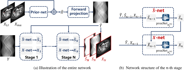
Figure 1: (a) The proposed network architecture consists of a Prior-net, $N$-stage $\widetilde{S}$-net, and $N$-stage $X$-net. It outputs the normalized sinogram $\widetilde{S}_{N}$, sinogram $S_{N}$, and image $X_{N}$. (b) The detailed structure at the $n$-th stage, in which $\widetilde{S}_{n}$ and $X_{n}$ are successively updated by $\widetilde{S}$-net and $X$-net, respectively, based on the algorithm in Eqs. (7)(9).

Training Loss. We adopt the mean square error (MSE) for the extracted sinogram $\widetilde{Y}\odot\widetilde{S}_{n}$ and image $X_{n}$ at every stage as the training objective function:

$$\mathcal{L}=\sum_{n=0}^{N}\beta_{n}\left\|X_{n}-X_{gt}\right\|_{F}^{2}\odot(1-M)+\gamma\left(\sum_{n=1}^{N}\beta_{n}\left\|\widetilde{Y}\odot\widetilde{S}_{n}-Y_{gt}\right\|_{F}^{2}\right),$$ (10)

where $X_{gt}$ and $Y_{gt}$ are ground truth image and metal-free sinogram, respectively. We simply set $\beta_{N}=1$ to make the outputs at the final stage play a dominant role, and $\beta_{n}=0.1$ ($n=0,\cdots,N-1$) to supervise each middle stage. $\gamma$ is a hyperparamter to balance the weight of different loss items and we empirically set it as 0.1. We initialize $X_{0}$ by passing $X_{LI}$ through a proximal network $\text{proxNet}_{\theta_{x}^{(0)}}$.

3 Experimental Results

Synthesized Data. Following the simulation protocol in [28], we randomly select a subset from the DeepLesion [27] to synthesize metal artifact data. The metal masks are from [32], which contain 100 metallic implants with different shapes and sizes. We choose 1,000 images and 90 metal masks to synthesize the training samples, and pair the additional 200 CT images from 12 patients with the remaining 10 metal masks to generate 2,000 images for testing. The sizes of the 10 metallic implants for test data are: [2061, 890, 881, 451, 254, 124, 118, 112, 53, 35] in pixels. Consistent to [13, 15], we simply put the adjacent sizes into one group when reporting MAR performance. We adopt the procedures widely used by existing studies [32, 12, 13, 28, 15] to simulate $Y$ and $X_{ma}$. All the CT images are resized to $416\times 416$ pixels and 640 projection views are uniformly spaced in 360 degrees. The resulting sinograms are of the size $N_{b}\times N_{p}$ as $641\times 640$.

Clinical Data. We further assess the feasibility of the proposed InDuDoNet on a clinical dataset, called CLINIC-metal [14], for pelvic fracture segmentation. The dataset includes 14 testing volumes labeled with multi-bone, i.e., sacrum, left hip, right hip, and lumbar spine. The clinical images are resized and processed using the same protocol to the synthesized data. Similar to [12, 28], the clinical metal masks are segmented with a thresholding (2,500 HU).

Evaluation Metrics. The peak signal-to-noise ratio (PSNR) and structured similarity index (SSIM) with the code from [32] are adopted to evaluate the performance of MAR. Since we perform the downstream multi-class segmentation on the CLINIC-metal dataset to assess the improvement generated by different MAR approaches to clinical applications, the Dice coefficient (DC) is adopted as the metric for the evaluation of segmentation performance.

Training Details. Based on a NVIDIA Tesla V100-SMX2 GPU, we implement our network with PyTorch [19] and differential operations $\mathcal{P}$ and $\mathcal{P}^{T}$ in ODL library. We adopt the Adam optimizer with ($\beta_{1}$, $\beta_{2}$)=(0.5, 0.999). The initial learning rate is $2\times 10^{-4}$ and divided by 2 every 40 epochs. The total epoch is 100 with a batch size of 1. Similar to [28], in each training iteration, we randomly select an image and a metal mask to synthesize a metal-affected sample.

Table 1: Effect of the total stage number $N$ on the performance of the proposed InDuDoNet on synthesized data with PSNR (dB) and SSIM.

$N$	Large Metal     $\longrightarrow$     Small Metal					Average
$N$=0	28.91/0.9280	30.42/0.9400	34.45/0.9599	36.72/0.9653	37.18/0.9673	33.54/0.9521
$N$=1	34.10/0.9552	35.91/0.9726	38.48/0.9820	39.94/0.9829	40.39/0.9856	37.76/0.9757
$N$=3	33.46/0.9564	37.14/0.9769	40.33/0.9868	42.55/0.9896	42.68/0.9908	39.23/0.9801
$N$=6	34.59/0.9764	38.95/0.9890	42.28/0.9941	44.09/0.9945	45.09/0.9953	41.00/0.9899
$N$=10	36.74/0.9801	39.32/0.9896	41.86/0.9931	44.47/0.9942	45.01/0.9948	41.48/0.9904
$N$=12	36.52/0.9709	40.01/0.9896	42.66/0.9955	44.17/0.9960	44.84/0.9967	41.64/0.9897

3.1 Ablation Study

Table 1 lists the performance of our framework under different stage number $N$. The $N=0$ entry means that the initialization $X_{0}$ is directly regarded as the reconstruction result. Taking $N=0$ as the baseline, we can find that with only one stage ($N=1$), the MAR performance yielded by our proposed InDuDoNet is already evidently improved, which validates the essential role of the mutual learning between $\widetilde{S}$-net and $X$-net. When $N=12$, the SSIM is slightly lower than that of $N=10$. The underlying reason is that the more stages cause a deeper network and may suffer from gradient vanishing. Hence, for better performance and fewer network parameters, we choose $N=10$ in all our experiments.

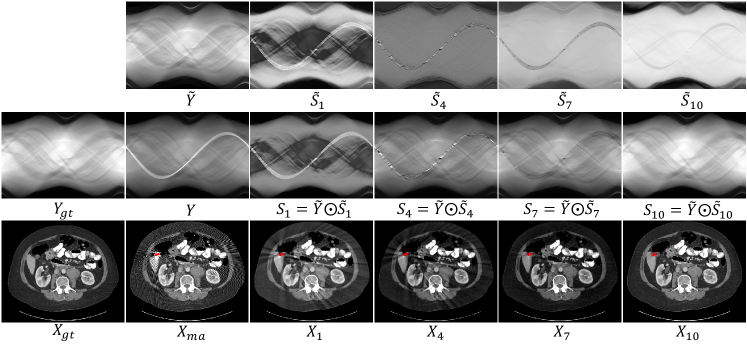
Figure 2: The recovery normalization coefficient $\widetilde{Y}$, normalized sinogram $\widetilde{S}_{n}$, sinogram $S_{n}$, and image $X_{n}$ at different stages ($N$=10). The red pixels stand for metallic implant.

Table 2: PSNR (dB) and SSIM of different MAR methods on synthesized data.

Methods	Large Metal     $\longrightarrow$     Small Metal					Average
Input	24.12/0.6761	26.13/0.7471	27.75/0.7659	28.53/0.7964	28.78/0.8076	27.06/0.7586
LI [10]	27.21/0.8920	28.31/0.9185	29.86/0.9464	30.40/0.9555	30.57/0.9608	29.27/0.9347
NMAR [17]	27.66/0.9114	28.81/0.9373	29.69/0.9465	30.44/0.9591	30.79/0.9669	29.48/0.9442
CNNMAR [32]	28.92/0.9433	29.89/0.9588	30.84/0.9706	31.11/0.9743	31.14/0.9752	30.38/0.9644
DuDoNet [13]	29.87/0.9723	30.60/0.9786	31.46/0.9839	31.85/0.9858	31.91/0.9862	31.14/0.9814
DSCMAR [28]	34.04/0.9343	33.10/0.9362	33.37/0.9384	32.75/0.9393	32.77/0.9395	33.21/0.9375
DuDoNet++ [15]	36.17/0.9784	38.34/0.9891	40.32/0.9913	41.56/0.9919	42.08/0.9921	39.69/0.9886
InDuDoNet (Ours)	36.74/0.9801	39.32/0.9896	41.86/0.9931	44.47/0.9942	45.01/0.9948	41.48/0.9904

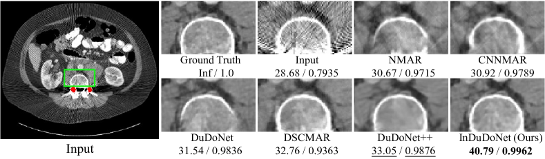
Figure 3: Comparison for medium metallic implants. PSNR (dB)/SSIM below is for reference. The display window is [-175, 275] HU. The red pixels stand for metallic implants.

Model Verification. We conduct a model verification experiment to present the mechanism underlying the network modules ($\widetilde{S}$-net and $X$-net). The evaluation results are shown in Fig. 2. The normalized sinogram $\widetilde{S}_{n}$, sinogram $S_{n}$, and CT image $X_{n}$ generated at different stages ($n=1,4,7,10$) are presented on the first, second and third rows, respectively. It can be observed that the metal trace region in $\widetilde{S}_{n}$ is gradually flattened as $n$ increases, which correspondingly ameliorates the sinogram $S_{n}$. Thus, the metal artifacts contained in the CT image $X_{n}$ are gradually removed. The results verify the design of our interpretable iterative learning framework—the mutual promotion of $\widetilde{S}$-net and $X$-net enables the proposed InDuDoNet to achieve MAR along the direction specified by Eq. (4).

Table 3: The Dice coefficient (DC) results on the downstream segmentation task.

Bone	Input	LI	NMAR	CNNMAR	DuDoNet	DSCMAR	DuDoNet++	InDuDoNet
Sacrum	0.9247	0.9086	0.9151	0.9244	0.9326	0.9252	0.9350	0.9348
Left hip	0.9543	0.9391	0.9427	0.9485	0.9611	0.9533	0.9617	0.9630
Right hip	0.8747	0.9123	0.9168	0.9250	0.9389	0.9322	0.9379	0.9421
Lumbar spine	0.9443	0.9453	0.9464	0.9489	0.9551	0.9475	0.9564	0.9562
Average DC	0.9245	0.9263	0.9303	0.9367	0.9469	0.9396	0.9478	0.9490

3.2 Performance Evaluation

Synthesized Data. We compare the proposed InDuDoNet with current state-of-the-art (SOTA) MAR approaches, including traditional LI [10] and NMAR [17], DL-based CNNMAR [32], DuDoNet [13], DSCMAR [28], and DuDoNet++ [15]. For LI, NMAR, and CNNMAR, we directly use the released code and model. We re-implement DuDoNet, DSCMAR, and DuDoNet++, since there is no official code. Table 2 reports the quantitative comparison. We can observe that most of DL-based methods consistently outperform the conventional LI and NMAR, showing the superiority of data-driven deep CNN for MAR. The dual enhancement approaches (i.e., DuDoNet, DSCMAR, and DuDoNet++) achieve higher PSNR than the sinogram-enhancement-only CNNMAR. Compared to DuDoNet, DSCMAR, and DuDoNet++, our dual-domain method explicitly embeds the physical CT imaging geometry constraints into the mutual learning between spatial and Radon domains, i.e., jointly regularizing the sinogram and CT image recovered at each stage. Hence, our method achieves the highest PSNRs and SSIMs for all metal sizes as listed. The visual comparisons are shown in Fig. 3.⁴

Clinical Data. We further evaluate all MAR methods on clinical downstream pelvic fracture segmentation task using the CLINIC-metal dataset. A U-Net is firstly trained using the clinical metal-free dataset (CLINIC [14]) and then tested on the metal-artifact-reduced CLINIC-metal CT images generated by different MAR approaches. The segmentation accuracy achieved by the metal-free-trained U-Net is reported in Table 3. We can observe that in average, our method finely outperforms other SOTA approaches. This comparison fairly demonstrates that our network generalizes well for clinical images with unknown metal materials and geometries and is potentially useful for clinical applications.

4 Conclusion

In this paper, we have proposed a joint spatial and Radon domain reconstruction model for the metal artifact reduction (MAR) task and constructed an interpretable network architecture, namely InDuDoNet, by unfolding an iterative optimization algorithm with only simple computations involved. Extensive experiments were conducted on synthesized and clinical data. The experimental results demonstrated the effectiveness of our dual-domain MAR approach as well as its superior interpretability beyond current SOTA deep MAR networks.

4.0.1 Acknowledgements.

This research was supported by National Key R&D Program of China (2020YFA0713900), the Macao Science and Technology Development Fund under Grant 061/2020/A2, Key-Area Research and Development Program of Guangdong Province, China (No. 2018B010111001), the Scientific and Technical Innovation 2030-“New Generation Artificial Intelligence” Project (No. 2020AAA0104100), the China NSFC projects (62076196, 11690011,61721002, U1811461).

Supplementary Material

Table 4: Comparison of network parameter and testing time. The average inference time is computed on 2000 images with size $416\times 416$ based on a NVIDIA Tesla V100-SMX2 GPU.

Methods	Network Parameters#	Test Time (Seconds)	Average PSNR (dB)/SSIM
DSCMAR	25,834,251	0.3638	33.21/0.9375
DuDoNet++	25,983,627	0.8062	39.69/0.9886
InDuDoNet ($N$=6)	4,541,060	0.3526	41.00/0.9892
InDuDoNet ($N$=10)	5,174,936	0.5116	41.48/0.9904

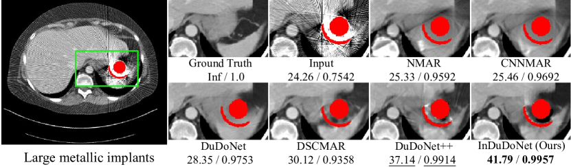
Figure 4: From the regions around the red metallic implant, we can observe that our method preserves more tissue structures and recovers anatomically more faithful image.

Figure 5: Comparison of different dual-domain-enhancement-based MAR methods. RMSE for sinogram and PSNR (dB)/SSIM for image below are for reference.

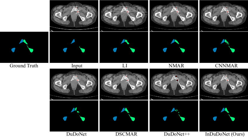
Figure 6: $1^{\text{st}}$ row is the generalization result on a CLINIC-metal CT image and $2^{\text{nd}}$ row is the segmentation result. The clinical metal masks are colored in red for better visualization. As observed, comparison methods with the inaccurate recovery of right hip, such as residual metal artifacts or missing structure, have the unsatisfactory segmentation results. However, the restored image by our method shows more credible contents with more details, which effectively promotes the segmentation performance.

References

- [1] Beck, A., Teboulle, M.: A fast iterative shrinkage-thresholding algorithm for linear inverse problems. SIAM Journal on Imaging Sciences 2(1), 183–202 (2009)
- [2] Chang, Z., Ye, D.H., Srivastava, S., Thibault, J.B., Sauer, K., Bouman, C.: Prior-guided metal artifact reduction for iterative X-ray computed tomography. IEEE Transactions on Medical Imaging 38(6), 1532–1542 (2018)
- [3] De Man, B., Nuyts, J., Dupont, P., Marchal, G., Suetens, P.: Metal streak artifacts in X-ray computed tomography: A simulation study. IEEE Transactions on Nuclear Science 46(3), 691–696 (1999)
- [4] Donoho, D.L.: De-noising by soft-thresholding. IEEE Transactions on Information Theory 41(3), 613–627 (1995)
- [5] Ghani, M.U., Karl, W.C.: Fast enhanced CT metal artifact reduction using data domain deep learning. IEEE Transactions on Computational Imaging 6, 181–193 (2019)
- [6] Gjesteby, L., Yang, Q., Xi, Y., Zhou, Y., Zhang, J., Wang, G.: Deep learning methods to guide CT image reconstruction and reduce metal artifacts. In: Medical Imaging 2017: Physics of Medical Imaging. vol. 10132, p. 101322W. International Society for Optics and Photonics (2017)
- [7] He, K., Zhang, X., Ren, S., Sun, J.: Deep residual learning for image recognition. In: Proceedings of the IEEE Conference on Computer Vision and Pattern Recognition. pp. 770–778 (2016)
- [8] Huang, X., Wang, J., Tang, F., Zhong, T., Zhang, Y.: Metal artifact reduction on cervical CT images by deep residual learning. Biomedical Engineering Online 17(1), 1–15 (2018)
- [9] Ji, W., Yu, S., Wu, J., Ma, K., Bian, C., Bi, Q., Li, J., Liu, H., Cheng, L., Zheng, Y.: Learning calibrated medical image segmentation via multi-rater agreement modeling. In: Proceedings of the IEEE/CVF Conference on Computer Vision and Pattern Recognition. pp. 12341–12351 (2021)
- [10] Kalender, W.A., Hebel, R., Ebersberger, J.: Reduction of CT artifacts caused by metallic implants. Radiology 164(2), 576–577 (1987)
- [11] Liao, H., Lin, W.A., Huo, Z., Vogelsang, L., Sehnert, W.J., Zhou, S.K., Luo, J.: Generative mask pyramid network for CT/CBCT metal artifact reduction with joint projection-sinogram correction. In: International Conference on Medical Image Computing and Computer Assisted Intervention. pp. 77–85 (2019)
- [12] Liao, H., Lin, W.A., Zhou, S.K., Luo, J.: ADN: Artifact disentanglement network for unsupervised metal artifact reduction. IEEE Transactions on Medical Imaging 39(3), 634–643 (2019)
- [13] Lin, W.A., Liao, H., Peng, C., Sun, X., Zhang, J., Luo, J., Chellappa, R., Zhou, S.K.: DuDoNet: Dual domain network for CT metal artifact reduction. In: Proceedings of the IEEE/CVF Conference on Computer Vision and Pattern Recognition. pp. 10512–10521 (2019)
- [14] Liu, P., Han, H., Du, Y., Zhu, H., Li, Y., Gu, F., Xiao, H., Li, J., Zhao, C., Xiao, L., et al.: Deep learning to segment pelvic bones: Large-scale CT datasets and baseline models. arXiv preprint arXiv:2012.08721 (2020)
- [15] Lyu, Y., Lin, W.A., Liao, H., Lu, J., Zhou, S.K.: Encoding metal mask projection for metal artifact reduction in computed tomography. In: International Conference on Medical Image Computing and Computer-Assisted Intervention. pp. 147–157 (2020)
- [16] Mehranian, A., Ay, M.R., Rahmim, A., Zaidi, H.: X-ray CT metal artifact reduction using wavelet domain sparse regularization. IEEE Transactions on Medical Imaging 32(9), 1707–1722 (2013)
- [17] Meyer, E., Raupach, R., Lell, M., Schmidt, B., Kachelrieß, M.: Normalized metal artifact reduction (NMAR) in computed tomography. Medical Physics 37(10), 5482–5493 (2010)
- [18] Park, H.S., Lee, S.M., Kim, H.P., Seo, J.K., Chung, Y.E.: CT sinogram-consistency learning for metal-induced beam hardening correction. Medical Physics 45(12), 5376–5384 (2018)
- [19] Paszke, A., Gross, S., Chintala, S., Chanan, G., Yang, E., DeVito, Z., Lin, Z., Desmaison, A., Antiga, L., Lerer, A.: Automatic differentiation in pytorch (2017)
- [20] Ronneberger, O., Fischer, P., Brox, T.: U-net: Convolutional networks for biomedical image segmentation. In: International Conference on Medical Image Computing and Computer Assisted Intervention. pp. 234–241 (2015)
- [21] Wang, G., Ye, J.C., Mueller, K., Fessler, J.A.: Image reconstruction is a new frontier of machine learning. IEEE Transactions on Medical Imaging 37(6), 1289–1296 (2018)
- [22] Wang, H., Wu, Y., Xie, Q., Zhao, Q., Liang, Y., Zhang, S., Meng, D.: Structural residual learning for single image rain removal. Knowledge-Based Systems 213, 106595 (2021)
- [23] Wang, H., Xie, Q., Zhao, Q., Meng, D.: A model-driven deep neural network for single image rain removal. In: Proceedings of the IEEE/CVF Conference on Computer Vision and Pattern Recognition. pp. 3103–3112 (2020)
- [24] Wang, H., Yue, Z., Xie, Q., Zhao, Q., Zheng, Y., Meng, D.: From rain generation to rain removal. In: Proceedings of the IEEE/CVF Conference on Computer Vision and Pattern Recognition. pp. 14791–14801 (2021)
- [25] Wang, J., Zhao, Y., Noble, J.H., Dawant, B.M.: Conditional generative adversarial networks for metal artifact reduction in CT images of the ear. In: International Conference on Medical Image Computing and Computer Assisted Intervention. pp. 3–11 (2018)
- [26] Xie, Q., Zhou, M., Zhao, Q., Xu, Z., Meng, D.: MHF-net: An interpretable deep network for multispectral and hyperspectral image fusion. IEEE Transactions on Pattern Analysis and Machine Intelligence (2020)
- [27] Yan, K., Wang, X., Lu, L., Zhang, L., Harrison, A.P., Bagheri, M., Summers, R.M.: Deep lesion graphs in the wild: Relationship learning and organization of significant radiology image findings in a diverse large-scale lesion database. In: Proceedings of the IEEE Conference on Computer Vision and Pattern Recognition. pp. 9261–9270 (2018)
- [28] Yu, L., Zhang, Z., Li, X., Xing, L.: Deep sinogram completion with image prior for metal artifact reduction in CT images. IEEE Transactions on Medical Imaging 40(1), 228–238 (2020)
- [29] Yue, Z., Yong, H., Zhao, Q., Zhang, L., Meng, D.: Variational image restoration network. arXiv preprint arXiv:2008.10796 (2020)
- [30] Zhang, H., Dong, B., Liu, B.: A reweighted joint spatial-radon domain CT image reconstruction model for metal artifact reduction. SIAM Journal on Imaging Sciences 11(1), 707–733 (2018)
- [31] Zhang, H., Wang, L., Li, L., Cai, A., Hu, G., Yan, B.: Iterative metal artifact reduction for X-ray computed tomography using unmatched projector/backprojector pairs. Medical Physics 43(6Part1), 3019–3033 (2016)
- [32] Zhang, Y., Yu, H.: Convolutional neural network based metal artifact reduction in X-ray computed tomography. IEEE Transactions on Medical Imaging 37(6), 1370–1381 (2018)