Remote sensing and faithful quantum teleportation through non-localized qubits

Abstract

One of the most important applications of quantum physics is quantum teleportation, the possibility to transfer quantum states over arbitrary distances. In this paper, we address the idea of remote sensing in a teleportation scenario with topological qubits more robust against noise. We also investigate the enhancement of quantum teleportation through non-local characteristics of the topological qubits. In particular, we show that how this nonlocal property, helps us to achieve near-perfect quantum teleportation even with mixed quantum states. Considering the limitations imposed by decoherence and the subsequent mixedness of the resource state, we find that our results may solve important challenges in realizing faithful teleportation over long distances.

I Introduction

Quantum teleportation, describing the transfer of an unknown quantum state over a long distance, constitutes a fundamental problem due to unavoidable transportation losses in combination with the no-cloning theorem Wootters and Zurek (1982). First highlighted by Bennett et al. Bennett et al. (1993), it has since evolved into an active and interesting area of research and is now recognized as an significant tool for many quantum protocols such as measurement-based quantum computing Raussendorf and Briegel (2001), quantum repeaters Sangouard et al. (2011), and fault-tolerant quantum computation Gottesman and Chuang (1999). The experiments have been first implemented by photons Bouwmeester et al. (1997), later with various systems such as trapped ions Riebe et al. (2004); Barrett et al. (2004), atomic ensembles Sherson et al. (2006), as well as with high-frequency phonons Hou et al. (2016) and several others Pirandola et al. (2015); Kumar et al. (2020); Liu et al. (2020); Langenfeld et al. (2021).

High-precision parameter estimation is a fundamental task throughout science. Generally speaking, there are two different scenarios for quantum parameter estimation in the presence of noises Holevo (1978); Giovannetti et al. (2004); Paris (2009); Giovannetti et al. (2011); Liu et al. (2019); Tóth and Apellaniz (2014); Polino et al. (2020); Pirandola et al. (2018); Bongs et al. (2019); Pezzè et al. (2018). In both approaches, the most important goals is to investigate the optimized measurement strategy such that as much information as possible about some parameter is achieved. In the first scenario, a quantum probe, with known initial state, is transmitted through a quantum channel, encoding the parameter of interest into the quantum state of the system, and then the output state is measured to extract an estimate from measurement results. However, in the other standard scenario, the information about the quantity of interest is initially encoded into the system state and then this information carrier is transmitted through a quantum noisy channel; finally, the measurement process is implemented.

We investigate the first aforementioned scenario where the information about the strength of the coupling between a topological qubit and its environment, is encoded by a teleportation channel Pirandola et al. (2015) into the state of the teleported qubits, leading to idea of remote sensing. This strategy is applied when our metrological setup is not accessible at a special place and we need to estimate some unknown parameter at that location without moving the devices. Experimental setups for teleportation-based quantum information processing with Majorana zero modes have been proposed in Vijay and Fu (2016).

If the probes are classically correlated and noninteracting, as a consequence of the central limit theorem, the mean-squared error of the estimate decreases as $1/N$, in which $N$ denotes the number of probes. This best scaling achievable through a classical probe is known as the standard quantum limit. Quantum metrology aims to enhance estimation by exploiting quantum correlations between probes Brask et al. (2015). In the absence of decoherence, it is well known that quantum resources allow for a quadratic improvement in precision over the standard quantum limit. However, in realistic evolution the presence of decoherence effects is unavoidable, and hence there is currently much effort to investigate exactly when and how quantum resources such as entanglement allow estimation to be improved in the presence of noises Wang et al. (2018); Braun et al. (2018); Liu et al. (2021); Rangani Jahromi (2020, 2019). We exploit this scenario through entangled teleported qubits realized by Majorana modes for remote quantum sensing of their couplings with the input environment. Estimation the system-environment coupling strength helps us to determine whether we can apply specific approximations in the theoretical model or not Hu et al. (1992); Boyanovsky et al. (2005). More importantly, the strength of the coupling is a significant parameter to control the decoherence effects Ho et al. (2014); Liu et al. (2013); Wu (2014). Moreover, in many-body quantum systems, changing the coupling constant may drive the system into different phases Invernizzi et al. (2008). These reasons motivate us to estimate the coupling constant of an interacting Hamiltonian not corresponding to any observable of the system, and hence it cannot be measured directly.

It has been shown that the topological quantum computation Freedman et al. (2003) is one of the most exciting approaches to constructing a fault-tolerant quantum computer Nayak et al. (2008). Particularly, there are novel kinds of topologically ordered states, such as topological insulators and superconductors Fu and Kane (2008); Hasan and Kane (2010); Qi and Zhang (2011), easy to realize physically. The most interesting excitations for these important systems are the Majorana modes, localized on topological defects, which obey the non-Abelian anyonic statistics Wilczek (2009); Arovas et al. (1984); Ivanov (2001).

One of the simplest scenarios for realization of Majorana modes are those appearing at the edges of the Kitaev’s spineless p-wave superconductor chain model Kitaev (2001); Sau et al. (2010); Alicea (2010); Thakurathi et al. (2014) where two far separated endpoint Majorana modes can compose a topological qubit. The most significant characteristic of the topological qubit is its non-locality, since the two Majorana modes are far separated. This non-local property makes topological qubits interact with the environment more unpredictably than the usual local qubits Ho et al. (2014). Motivated by this, we study the implementation of quantum information tasks usually investigated for local qubits, such as quantum teleportation and quantum parameter estimation, through non-local qubits.

A continuous process is called Markovian if, starting from any initial state, its dynamics can be determined unambiguously from the initial state. Non-Markovianity Rivas et al. (2014); Breuer (2012) is inherently connected to the two-way exchange of information between the system and the environment; a Markovian description of dynamics is legitimate, even if only as an approximation, whenever the observed time scale of the evolution is much larger than the correlation time characterizing the interaction between system and its environment. Non-Markovianity is a complicated phenomenon affecting the system both in its informational and dynamical features. For a recent review of the witnesses and approaches to characterize non-Markovianity we refer to Li et al. (2018).

In this paper we consider remote sensing through quantum teleportation implemented by non-local Majorana modes realizing two topological qubits independently coupled to non-Markovian Ohmic-like reservoirs. We show that how environmental control parameters, i.e., cutoff frequency, Ohmicity parameter, and the coupling strength, applied at the destination of teleportation, affect the remote sensing, the quality of teleportation and quantum correlations between teleported non-local qubits. In particular, the quantum control to achieve near-perfect teleportation is discussed.

This paper is organized as follows: In Section II, we present a brief review of the standard quantum teleportation, quantum metrology, measure of quantum resources and Hilbert-Schmidt speed. The model and its non-Markovian characteristics are introduced in Section III. Moreover, the scenario of teleportation and remote sensing are discussed in Sec. IV. Finally in Section V, the main results are summarized.

II PRELIMINARIES

In this section we review the most important concepts discussed in this paper.

II.0.1 Standard quantum teleportation

The main idea of quantum teleportation is transferring quantum information from the sender (Alice) to the receiver (Bob) through entangled pairs. In the standard protocol Bowen and Bose (2001), the teleportation is realized by a two-qubit mixed state $\rho_{\text{res}}$, playing the role of the resource, and is modeled by a generalized depolarizing channel $\Lambda_{\text{res}}$, acting on an input state $\rho_{\text{in}}$ which is the single-qubit state to be teleported, i.e.,

$$\rho_{\text{out}}=\Lambda_{\text{res}}\left(\rho_{\text{in}}\right),~{}~{}~{}~{}~{}~{}~{}~{}~{}~{}~{}~{}~{}$$

$$=\sum^{3}_{i=0}\text{Tr}\left[\mathcal{B}_{i}\rho_{\text{\text{res}}}\right]\sigma_{i}\rho_{\text{in}}\sigma_{i},$$ (1)

where $\mathcal{B}_{i}$’s denote the Bell states associated with the Pauli matrices $\sigma_{i}$’s by the following relation

$$\mathcal{B}_{i}=\left(\sigma_{0}\otimes\sigma_{i}\right)\mathcal{B}_{0}\left(\sigma_{0}\otimes\sigma_{i}\right);\;i=1,2,3,$$ (2)

in which $\sigma_{0}=I$, $\sigma_{1}=\sigma_{x}$, $\sigma_{2}=\sigma_{y}$, $\sigma_{3}=\sigma_{z}$, and $I$ is the $2\times 2$ identity matrix. For any arbitrary two-qubit system, each described by basis $\left\{\Ket{0},\Ket{1}\right\}$, we have $\mathcal{B}_{0}=\frac{1}{2}\left(\Ket{00}+\Ket{11}\right)\left(\Bra{00}+\Bra{11}\right)$, without loss of the generality.

Generalizing the above scenario, Lee and Kim Lee and Kim (2000a) investigated the standard teleportation of an unknown entangled state. In this protocol, the output state of the teleportation channel is found to be

$$\rho_{\text{out}}=\sum_{ij}p_{ij}\left(\sigma_{i}\otimes\sigma_{j}\right)\rho_{\text{in}}\left(\sigma_{i}\otimes\sigma_{j}\right),\ i,j=0,x,y,z,$$ (3)

where $p_{ij}=\text{Tr}\left[\mathcal{B}_{i}\rho_{\text{res}}\right]\text{Tr}\left[\mathcal{B}_{j}\rho_{\text{res}}\right]$ and $\sum p_{ij}=1$.

II.0.2 Quantum estimation theory

First we briefly review the principles of classical estimation theory and the tools that it provides to compute the bounds to precision of any quantum metrology process. In an estimation problem we intend to infer the value of a parameter $\lambda$ by measuring a related quantity $X$. In order to solve the problem, one should find an estimator $\hat{\lambda}\equiv\hat{\lambda}(x_{1},x_{2},...)$, i.e., a real function of the measurement outcomes $\left\{x_{k}\right\}$ to the space of the possible values of the parameter $\lambda$. In the classical scenario, the variance $\text{Var}(\lambda)=E[\hat{\lambda}^{2}]-E[\hat{\lambda}]^{2}$ of any unbiased estimator, in which $E[...]$ represents the mean with respect to the $n$ identically distributed random variables $x_{i}$, satisfies the Cramer-Rao inequality $\text{Var}(\lambda)\geq\dfrac{1}{MF_{\lambda}}$. It provides a lower bound on the variance in terms of the number of independent measurements $M$ and the Fisher information (FI) $F(\lambda)$

$$F_{\lambda}=\sum_{x}\dfrac{[\partial_{\lambda}p(x|\lambda)]^{2}}{p(x|\lambda)},$$ (4)

where $p(x|\lambda)$ denotes the conditional probability of achieving the value $x$ when the parameter has the value $\lambda$. Here it is assumed that the eigenvalue spectrum of observable $X$ is discrete. If it is continuous, the summation in Eq. (60) must be replaced by an integral.

In the quantum scenario $p(x|\lambda)=\text{Tr}\left[\rho P_{x}\right]$, where $\rho$ represents the state of the quantum system and $P_{x}$ denotes the probability operator-valued measure (POVM) describing the measurement. In summary, it is possible to extract the value of the physical parameter, intending to estimate it, by measuring an observable $X$ and then performing statistical analysis on the measurements results. An efficient estimator at least asymptotically saturates the Cramer-Rao bound.

Clearly, various observables give rise to miscellaneous probability distributions, leading to different FIs and hence to different precisions for estimating $\lambda$. The quantum Fisher information (QFI), the ultimate bound to the precision, is achieved by maximizing the FI over the set of the observables. It is known that the set of projectors over the eigenstates of the SLD forms an optimal POVM. The QFI of an unknown parameter $\lambda$ encoded into the quantum state $\rho\left(\lambda\right)$ is given by Helstrom (1969); Braunstein et al. (1996)

$$\mathcal{F}_{\lambda}=\text{Tr}\left[\rho\left(\lambda\right)L^{2}\right]=\text{Tr}\left[\left(\partial_{\lambda}\rho\left(\lambda\right)\right)L\right],$$ (5)

in which $L$ denotes the symmetric logarithmic derivative (SLD) given by $\partial_{\lambda}\rho\left(\lambda\right)=\frac{1}{2}\left(L\rho\left(\lambda\right)+\rho\left(\lambda\right)L\right),$ where $\partial_{\lambda}=\partial/\partial\lambda$.

Following the method presented in Jing et al. (2014); Liu et al. (2016) to calculate the QFI of block diagonal states $\rho=\bigoplus^{n}_{i=1}\rho_{i}$, where $\bigoplus$ denotes the direct sum, one finds that the SLD operator is also block diagonal and can be computed explicitly as $L=\bigoplus^{n}_{i=1}L_{i}$ in which $L_{i}$ represents the corresponding SLD operator for $\rho_{i}$. For 2-dimensional blocks, it is proved that the SLD operator for the $i$th block is expressed by Liu et al. (2016)

$$L_{i}=\frac{1}{\mu_{i}}\left[\partial_{x}\rho_{i}+\xi_{i}\rho^{-1}_{i}-\partial_{x}\mu_{i}\right].$$ (6)

in which $\xi_{i}=2\mu_{i}\partial_{x}\mu_{i}-\partial_{x}P_{i}/4$ where $\mu_{i}=\text{Tr}\left[\rho_{i}/2\right]$ and $P_{i}=\text{Tr}\left[\rho^{2}_{i}\right]$. When $\text{det}(\rho_{i})=0$, $\xi_{i}$ vanishes.

II.0.3 Quantum resources

In this subsection we introduce some important measures to quantify key resources which may be needed for implementing quantum information tasks.

Quantum entanglement

In bipartite qubit systems, the concurrence Wootters (1998); Bennett et al. (1996) is one of the most important measures used to quantify entanglement. Introducing the "spin flip" transformation given by

$$\rho\rightarrow\tilde{\rho}=(\sigma_{y}\otimes\sigma_{y})\rho^{*}(\sigma_{y}\otimes\sigma_{y}),$$ (7)

where $*$ denotes the complex conjugate, Wootters Wootters (1998) presented the following analytic expression for the concurrence of the mixed states of two-qubit systems:

$$C(\rho)=\text{max}(0,\lambda_{1}-\lambda_{2}-\lambda_{3}-\lambda_{4}),$$ (8)

where $\lambda_{i}$ are the square roots of the eigenvalues of $\rho\tilde{\rho}$ in decreasing order. The concurrence has the range from from 0 to 1. A quantum state with $C=0$ is separable. Moreover, when $C=1$, the state is maximally entangled. For a X state the concurrence has the form

$$C(\rho)=2\text{max}\left\{0,C_{1}(\rho),C_{2}(\rho)\right\},$$ (9)

where $C_{1}(\rho)=|\rho_{14}|-\sqrt{\rho_{22}\rho_{33}},C_{2}(\rho)=|\rho_{23}|-\sqrt{\rho_{11}\rho_{44}}$, and $\rho_{ij}$’s are the elements of density matrix.

Quantum coherence

Quantum coherence (QC), naturally a basis dependent concept identified by the presence of off-diagonal terms in the density matrix, is an important resource in quantum information theory (seeStreltsov et al. (2017) for a review). The reference basis can be determined by the physics of the problem under investigation or by the task for which the QC is required as a resource. Although different measures such as trace norm distance coherence Shao et al. (2015), $l_{1}$ norm, and relative entropy of coherence Baumgratz et al. (2014) are presented to quantify the QC of a quantum state, we adopt the $l_{1}$ norm which is easily computable. For a quantum state with the density matrix $\rho$, the $l_{1}$ norm measure of quantum coherence Baumgratz et al. (2014) quantifying the QC through the off diagonal elements of the density matrix in the reference basis, is given by

$$\mathcal{C}_{l_{1}}\left(\rho\right)=\sum_{i,j\atop i\neq j}|\rho_{ij}|.$$ (10)

In Ref. Yao et al. (2015) the authors investigated whether a basis-independent measure of QC can be defined or not. They found that the basis-free coherence is equivalent to quantum discord Ollivier and Zurek (2001), verifying the fact that coherence can be introduced as a form of quantum correlation in multi-partite quantum systems.

Quantum discord

Quantum discord (QD) Ollivier and Zurek (2001), defined as difference between total correlations and classical correlations Fanchini et al. (2017), represents the quantumness of the state of a quantum system. QD is a resource for certain quantum technologies Pirandola (2014), because it can be preserved for a long time even when entanglement exhibits a sudden death. Usually, computing QD for a general state is not easy because it involves the optimization of the classical correlations. Nevertheless, for a two-qubit $X$ state system, an easily computable expression of QD is given by Wang et al. (2010)

$$QD(\rho)=\text{min}\left(Q_{1},Q_{2}\right),$$ (11)

in which

$$Q_{j}=H\left(\rho_{11}+\rho_{33}\right)+\sum_{i=1}^{4}\lambda_{i}\text{log}_{2}\lambda_{i}+D_{j},~{}~{}~{}\left(j=1,2\right),~{}~{}~{}~{}~{}$$

$$D_{1}=H\left(\frac{1+\sqrt{\left[1-2\left(\rho_{33}+\rho_{44}\right)\right]^{2}+4\left(|\rho_{14}|+|\rho_{23}|\right)^{2}}}{2}\right),$$ (12)

$$D_{2}=-\sum_{i}\rho_{ii}\text{log}_{2}\rho_{ii}-H\left(\rho_{11}+\rho_{33}\right),~{}~{}~{}~{}~{}~{}~{}~{}~{}~{}~{}~{}~{}~{}~{}~{}~{}~{}~{}~{}~{}~{}~{}~{}~{}~{}$$

$$H\left(x\right)=-x\text{log}_{2}x-\left(1-x\right)\text{log}_{2}\left(1-x\right),~{}~{}~{}~{}~{}~{}~{}~{}~{}~{}~{}~{}~{}~{}~{}~{}~{}~{}~{}~{}~{}~{}~{}~{}$$

and $\lambda_{i}$’s represent the eigenvalues of the bipartite density matrix $\rho$.

II.0.4 Hilbert-Schmidt speed

First we consider the distance measure $d(p,q)$, defined as Gessner and Smerzi (2018) $[d(p,q)]^{2}=1/2\sum\limits_{x}|p_{x}-q_{x}|^{2},$ where $p=\{p_{x}\}_{x}$ and $q=\{q_{x}\}_{x}$, depending on parameter $\varphi$, represent the probability distributions, leading to the classical statistical speed $s[p(\varphi_{0})]=\dfrac{\mathrm{d}}{\mathrm{d}\varphi}\ d(p(\varphi_{0}+\varphi),p(\varphi_{0})).$ In order to extend these classical notions to the quantum case, one can consider a given pair of quantum states $\rho$ and $\sigma$, and write $p_{x}=\text{Tr}\left[E_{x}\rho\right]$ and $q_{x}=\text{Tr}\left[E_{x}\sigma\right]$ which denote the measurement probabilities corresponding to the positive-operator-valued measure (POVM) $\{E_{x}\geq 0\}$ satisfying $\sum\limits_{x}E_{x}=\mathbb{I}$ . Maximizing the classical distance $d(p,q)$ over all possible choices of POVMs Luo and Zhang (2004), we can obtain the corresponding quantum distance called the Hilbert-Schmidt distance $\delta_{HS}$ Ozawa (2000) given by $\delta_{HS}(\rho,\sigma)\equiv\max_{\{E_{x}\}}d(p,q)=\sqrt{\frac{1}{2}\text{Tr}[(\rho-\sigma)^{2}]}.$ Therefore, the Hilbert-Schmidt speed (HSS), the corresponding quantum statistical speed, is achieved by maximizing the classical statistical speed over all possible POVMs Paris (2009); Gessner and Smerzi (2018)

$$HS\!S\big{(}\rho(\varphi)\big{)}\equiv HS\!S_{\varphi} =\max_{\{E_{x}\}}\text{s}\big{[}p(\varphi)\big{]}$$

$$=\sqrt{\frac{1}{2}\text{Tr}\bigg{[}\bigg{(}\dfrac{\mathrm{d}\rho(\varphi)}{\mathrm{d}\varphi}\bigg{)}^{2}\bigg{]}}.$$ (13)

III Dynamics of the non-localized qubit realized by Majorana modes

We discuss the time evolution of a topological qubit realized by spatially-separated Majorana modes, and placed on top of an s-wave superconductor. The Majorana modes are generated at the endpoints of some nanowire with strong spin-orbit interaction, and are subject to an external magnetic field $\mathcal{B}$ along the wire axis direction. They are independently coupled to metallic nanowires via tunnel junctions such that the tunneling strengths are controllable through external gate voltages.

The total Hamiltonian can be written as Ho et al. (2014)

$$H=H_{S}+H_{E}+V$$ (14)

in which $H_{s}$ represents the Hamiltonian of the topological qubit. Assuming that the Majorana modes are zero-energy ones, we can put $H_{S}=0$. Furthermore, the Hamiltonian of the environment, composed of 1D electrons, is denoted by $H_{E}$ which can be written in terms of the electrons’s creation and annihilation operators, i.e., $\Xi^{\dagger}_{j}$, and $\Xi_{j}$, respectively. The noise affecting the topological qubit can be modelled as a fermionic Ohmic-like environment realized by placing a metallic nanowire close to the Majorana endpoint and described by spectral density $\rho_{spec}\propto\omega^{Q}$ with $Q\geq 0$. The environment is called Ohmic for $Q=1$, and super (sub)-Ohmic for $Q>1~{}(Q<1)$. A physical implementation of this kind of environment is the helical Luttinger liquids realized as interacting edge states of two-dimensional topological insulators Chao et al. (2013). Moreover, ignoring the weak coupling between the Majorana modes and the higher order terms involving greater numbers of Majorana modes, the system-environment interaction Hamiltonian is given by

$$V\simeq B(\gamma_{1}\mathcal{O}_{1}+\gamma_{2}\mathcal{O}_{2}),$$ (15)

in which $B$ is the real coupling strength between the Majorana modes and the environment, and $\mathcal{O}_{1(2)}$ denotes the composite operator of $\Xi^{\dagger}_{j}$, and $\Xi_{j}$. In addition, the localized Majorana modes $\gamma_{1}$ and $\gamma_{2}$ satisfy the following properties:

$$\gamma^{\dagger}_{a}=\gamma_{a},~{}~{}~{}\{\gamma_{a},\gamma_{b}\}=2\delta_{ab},$$ (16)

where $a,b=1,2$. $\gamma_{1,2}$ can be represented by:

$$\gamma_{1}=\sigma_{1},~{}~{}~{}\gamma_{2}=\sigma_{2},~{}~{}~{}\text{i}\gamma_{1}\gamma_{2}=\sigma_{3},$$ (17)

wherein $\sigma_{j}$’s denote the Pauli matrices. Besides, the two Majorana modes can be treated as a topological (non-local) qubit described by basis states $|0\rangle$ and $|1\rangle$ such that:

$$\frac{1}{2}(\gamma_{1}-\text{i}\gamma_{2})|0\rangle=|1\rangle,~{}~{}~{}~{}~{}\frac{1}{2}(\gamma_{1}+\text{i}\gamma_{2})|1\rangle=|0\rangle.$$ (18)

The fermionic Ohmic-like environment environment, composed of 1D electrons, is either Fermi or Luttinger liquid whose interaction strengths are characterized by the parameter $\kappa=(Q+1)/2$. Therefore, the larger $\kappa$, the stronger the correlation/interaction exhibited by the Luttinger liquid nanowire. It should be noted that $\kappa\equiv(K+1/K)/4$ in which $K$, representing the Luttinger parameter, can be roughly estimated as $K\thicksim(1+\dfrac{U}{2\epsilon_{F}})$ in which $\epsilon_{F}$ is the Fermi energy and $U$ denotes the characteristic Coulomb energy of the wire kane1992transport; Ho et al. (2014). Accordingly, the value of $\kappa$ and consequently $Q$ can be tuned by changing the effective attractive/repulsive short range interactions in the wire.

Assuming that the the Majorana qubit is initially prepared in the following state:

$$\varrho(0)=\left(\begin{array}[]{cc}\varrho_{11}(0)&\varrho_{12}(0)\\ \varrho_{21}(0)&\varrho_{22}(0)\\ \end{array}\right),$$ (19)

one can find that the reduced density matrix at time $t$ is given by (for details, see Ho et al. (2014)):

$$\varrho(t)=\frac{1}{2}\left(\begin{array}[]{cc}1+(2\varrho_{11}(0)-1)\alpha^{2}(t)&2\varrho_{12}(0)\alpha(t)\\ 2\varrho_{21}(0)\alpha(t)&1+(2\varrho_{22}(0)-1)\alpha^{2}(t)\\ \end{array}\right),$$ (20)

in which

$$\alpha(t)=\text{e}^{-2B^{2}|\beta|I_{Q}},~{}~{}~{}~{}~{}\beta\equiv\dfrac{-4\pi}{\Gamma(Q+1)}(\dfrac{1}{\varGamma_{0}})^{Q+1},$$ (21)

where $\varGamma_{0}$ denotes the cutoff frequency, appeared in the Green function for the fermionic environment, and $\Gamma(z)$ represents the Gamma function. Furthermore,

$$I_{Q}(t)=\left\{\begin{array}[]{rl}2\varGamma_{0}^{Q-1}\Gamma(\frac{Q-1}{2})\bigg{[}1-\,_{1}F_{1}\big{(}\frac{Q-1}{2};\frac{1}{2};-\frac{t^{2}\varGamma^{2}_{0}}{4}\big{)}\bigg{]}&~{}~{}~{}~{}~{}~{}~{}~{}\text{for}~{}Q\neq 1,\\ \frac{1}{2}t^{2}\varGamma^{2}_{0}\,{}_{2}F_{2}\bigg{(}\{1,1\};\{3/2,2\};-\frac{t^{2}\varGamma^{2}_{0}}{4}\bigg{)}&~{}~{}~{}~{}~{}~{}~{}~{}\text{for}~{}Q=1,\end{array}\right.$$ (22)

where $\,{}_{p}F_{q}$ represents the generalized hypergeometric function. It should be noted that $\varrho^{T}(0)$, describing the initial state of the total system, is assumed to be uncorrelated, i.e., $\varrho^{T}(0)=\varrho(0)\otimes\varrho_{E}$, where $\rho_{S}(0)$ and $\rho_{E}$ represent, respectively, the initial density matrix of the the topological qubit and that of the environment.

The trace norm defined by $\parallel\rho\parallel=\text{Tr}\sqrt{\rho^{\dagger}\rho}=\sum\limits_{k}\sqrt{\lambda_{k}}$, where $\lambda_{k}$’s represent the eigenvalues of $\rho^{\dagger}\rho$ can be used to define the trace distance Fanchini et al. (2017) $D(\rho^{1},\rho^{2})=\frac{1}{2}\parallel\rho^{1}-\rho^{2}\parallel$ an important measure of the distinguishability between two quantum states $\rho^{1}$ and $\rho^{2}$. This measure was applied by Breuer, Laine, and Piilo (BLP) Breuer et al. (2009) to define one of the most important characterization of non-Markovianity in quantum systems. They proposed that a non-Markovian process can be characterized by a backflow of information from the environment into the open system mathematically detected by the witness $\dot{D}\big{(}\rho^{1}(t),\rho^{2}(t)\big{)}>0$ in which $\rho^{i}(t)$ denotes the evolved state starting from the initial state $\rho^{i}(0)$, and the dot represents the time derivative.

In order to calculate the BLP measure of non-Markovianity, one has to find a specific pair of optimal initial states maximizing the time derivative of the trace distance. For any non-Markovian evolution of a one-qubit system, it is known that the maximal backflow of information occurs for a pair of pure orthogonal initial states corresponding to antipodal points on the surface of the Bloch sphere of the qubit. In Ref. Jahromi and Haseli (2020), the non-Markovian features of our model has been investigated and found that the optimal initial states are given by $\{|0\rangle,|1\rangle\}$, and the corresponding evolved trace distance is obtained as $D\big{(}\rho^{1}(t),\rho^{2}(t)\big{)}\equiv D(t)=\alpha^{2}(t)$.

Here we show that those features can also be extracted by another faithful witness of non-Markovianity recently proposed in Jahromi et al. (2020). According to this witness, at first we should compute the evolved density matrix $\varrho(t)$ corresponding to initial state $|\psi_{0}\rangle=\frac{1}{2}\bigg{(}\text{e}^{i\varphi}\ket{+}+\ket{-}\bigg{)}$. Here $\{\ket{+},\ket{-}\}$, constructing a complete and orthonormal set (basis) for the qubit, is usually associated with the computational basis. Then the positive changing rate of the Hilbert-Schmidt speed (HSS), i.e., $\dfrac{\text{d}HS\!S_{\varphi}(\varrho(t))}{\text{d}t}>0$ in which the HSS has been computed with respect to the initial phase $\varphi$, can identify the memory effects. This witness of non-Markovianity is in total agreement with the BLP witness, thus detecting the system-environment information backflows.

Considering the initial state $|\psi_{0}\rangle=\frac{1}{2}\bigg{(}\text{e}^{i\varphi}\ket{0}+\ket{1}\bigg{)}$ in our model, and using Eq. (II.0.4), we find that the HSS of $\varrho(t)$, obtained from Eq. (20), with respect to the phase parameter $\varphi$ is given by

$$HS\!S_{\varphi}(\varrho(t))\equiv HS\!S_{\varphi}(t)=\dfrac{\alpha(t)}{2},$$ (23)

leading to

$$HS\!S_{\varphi}(t)=\dfrac{\sqrt{D(t)}}{2}\Rightarrow\dfrac{\text{d}HS\!S_{\varphi}(t)}{\text{d}t}=\frac{1}{4\sqrt{D(t)}}\dfrac{\text{d}D(t)}{\text{d}t}.$$ (24)

Because the trace distance is a nonnegative quantity, the signs of $\dfrac{\text{d}D(t)}{\text{d}t}$ and $\dfrac{\text{d}HS\!S_{\varphi}}{\text{d}t}$ coincide and hence they exhibit the same qualitative dynamics.

This result verifies the fact that the HSS-based measure is in perfect agreement with the trace distance-based witness and can be used as an efficient as well as easily computable tool for detecting the non-Markovianity in our model.

A necessary condition which should be satisfied by a faithful witness of non-Markovianity is contractivity under Markovian dynamics. It should be noted that the noncontractivity of the Hilbert-Schmidt distance does not consequently lead to noncontractivity of the HSS. In more detail, as explained in Sec. II.0.4, the Hilbert-Schmidt distance is calculated by maximizing over all the possible choices of POVMs $\{E_{x}\}$ of the adopted distance measure, while the HSS is determined by maximization applied after the differentiation with respect to $\varphi$, starting from the corresponding distance measure. Because of these computational subtleties, from noncontractivity of the Hilbert-Schmidt distance we cannot deduce that the HSS is also noncontractive. Moreover, in Ref. Jahromi et al. (2020) we have demonstrated that the HSS is contractive in Hermitian systems.

IV teleportation using non-localized qubits

In this section, we investigate the scenario in which the non-localized qubits are used as the resource for teleportation of an entangled pair.

IV.1 Output state of the teleportation

Calculating the the eigenvalues and eigenvectors of the Choi matrix Leung (2003) of the map $\Phi_{t}$ satisfying the relationship $\Phi_{t}(\rho(0))=\rho(t)$, one can obtain the corresponding operator-sum representation $\varrho(t)=\sum_{i=1}^{4}K_{i}(t)\varrho(0)K_{i}(t)^{\dagger}$ where the Kraus operators $\{K_{i}(t)\}$ are given by Jahromi and Franco (2021)

$$K_{1}(t)=\left(\begin{array}[]{cc}\frac{\alpha-1}{2}&0\\ 0&\frac{1-\alpha}{2}\\ \end{array}\right),~{}K_{2}(t)=\left(\begin{array}[]{cc}\frac{\alpha+1}{2}&0\\ 0&\frac{\alpha+1}{2}\\ \end{array}\right),$$ (29)

$$K_{3}(t)=\left(\begin{array}[]{cc}0&\frac{\sqrt{1-\alpha^{2}}}{\sqrt{2}}\\ 0&0\\ \end{array}\right),~{}K_{4}(t)=\left(\begin{array}[]{cc}0&0\\ \frac{\sqrt{1-\alpha^{2}}}{\sqrt{2}}&0\\ \end{array}\right).$$ (34)

In the following, we take a system formed by two noninteracting non-localized qubits such that each of which locally interacts with its environment in Sec. III.

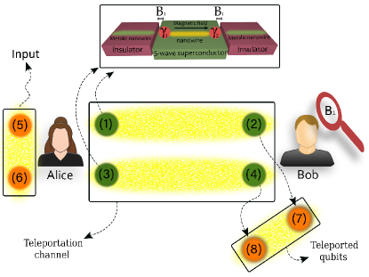
Figure 1: Sketch of the two-qubit noisy teleportation protocol through non-localized Majorana qubits. Qubits (1,2) and (3,4), representing two copies of the evolved noisy two-qubit system, are used as the resource channel for the protocol, and shared between Alice and Bob. The input qubits (5,6) which should be teleported, are manipulated in Alice’s location. After the protocol, Bob’s qubits, coming from the resource state, are transformed into qubits (7,8) representing the teleported qubits. Bob employs these qubits for remote sensing to estimate $B_{1}$, i.e., the strength of coupling between Alice’s Majorana qubit and its fermionic environment.

Because the environments are independent in our model, the Kraus operators, describing the dynamics of this composite system, are just the tensor products of Kraus operators acting on each of the qubits Nielsen and Chuang (2002). Therefore, assuming that the two-qubit system is prepared in the initial entangled state $\rho_{0}=|\Psi_{0}\rangle\langle\Psi_{0}|$ where

$$|\Psi_{0}\rangle=\cos(\vartheta/2)|00\rangle+\sin(\vartheta/2)|11\rangle.$$ (35)

we can find that the nonzero elements of the evolved density matrix $\rho(t)$ are given by

$$\rho_{1,1}(t)=\frac{1}{4}\left(\left(\text{$\alpha$}_{1}^{2}+\text{$\alpha$}_{2}^{2}\right)\cos(\vartheta)+\text{$\alpha$}_{1}^{2}\text{$\alpha$}_{2}^{2}+1\right),$$

$$\rho_{22}(t)=\frac{1}{4}\left(\left(\text{$\alpha$}_{1}^{2}-\text{$\alpha$}_{2}^{2}\right)\cos(\vartheta)-\text{$\alpha$}_{1}^{2}\text{$\alpha$}_{2}^{2}+1\right),$$ (36)

$$\rho_{33}(t)=\frac{1}{4}\left(\left(\text{$\alpha$}_{2}^{2}-\text{$\alpha$}_{1}^{2}\right)\cos(\vartheta)-\text{$\alpha$}_{1}^{2}\text{$\alpha$}_{2}^{2}+1\right),$$

$$\rho_{4,4}(t)=1-\bigg{(}\rho_{1,1}(t)+\rho_{2,2}(t)+\rho_{3,3}(t)\bigg{)},$$

$$\rho_{1,4}(t)=\frac{1}{2}\text{$\alpha$}_{1}\text{$\alpha$}_{2}\sin(\vartheta),$$

where $\alpha_{i}$ ($i=1,2$), presented in Eq. (21) for each qubit, includes the Ohmicity parameter $Q_{i}$, cutoff $\Gamma_{i}$, and coupling (tunneling) strength $B_{i}$.

Sharing two copies of this two-qubit system between Alice and Bob, as the resource or channel ($\rho(t)=\rho_{ch}$) for the quantum teleportation of the input state

$$|\psi_{in}\rangle=\text{cos}~{}\left(\frac{\theta}{2}\right)|10\rangle+e^{i\phi}~{}\text{sin}~{}\left(\frac{\theta}{2}\right)|01\rangle,$$ (37)

with $\ 0\leq\theta\leq\pi,\ 0\leq\varphi\leq 2\pi$, and following Kim and Lee’s two-qubit teleportation protocol Lee and Kim (2000b), we obtain the output state as

$$\rho_{\text{out}}(t)=\left(\begin{array}[]{cccc}\frac{1}{4}\left(1-\alpha^{4}\right)&0&0&0\\ 0&\frac{1}{4}\left(-2\alpha^{2}\cos\theta+\alpha^{4}+1\right)&\frac{1}{2}\alpha^{2}e^{i\phi}\sin\theta\sin^{2}\vartheta&0\\ 0&\frac{1}{2}\alpha^{2}e^{-i\phi}\sin\theta\sin^{2}\vartheta&\frac{1}{4}\left(2\alpha^{2}\cos\theta+\alpha^{4}+1\right)&0\\ 0&0&0&\frac{1}{4}\left(1-\alpha^{4}\right)\end{array}\right),$$ (38)

where $\alpha(t)=\alpha_{1}(t)\alpha_{2}(t)$. Extracting the results throughout this paper, we assume that the two-qubit states (35) and (37) are maximally entangled, i.e., $\theta=\vartheta=\pi/2$.

IV.2 Remote sensing through teleported qubits

We address the estimation of the coupling strength $B_{1}$ at Alice’s location, through the non-localized qubits, teleported to Bob’s location. It is an interesting model motivating investigation of making remote sensors (see Fig. 1).

The state of the two-qubit system, used for the remote sensing, is given by Eq. (38). It can be transformed into a block-diagonal form by changing the order of the basis vectors. Then, using Eq. (6), we find that the SLD, associated with the coupling strength, is obtained as

$$L(t)=\left(\begin{array}[]{cccc}\frac{4\alpha^{3}}{\alpha^{4}-1}&0&0&0\\ 0&\frac{4\left(-2\alpha^{3}\left(\sin^{2}\theta\right)\left(\sin^{4}\vartheta\right)+\alpha(\cos\theta)\left(-2\alpha^{2}(\cos\theta)+\alpha^{4}-1\right)+\alpha^{7}+\alpha^{3}\right)}{\left(\alpha^{4}+1\right)^{2}-4\alpha^{4}\left(\left(\sin^{2}\theta\right)\left(\vartheta\sin^{4}\right)+\cos^{2}\theta\right)}&-\frac{4\alpha\left(\alpha^{4}-1\right)e^{i\phi}(\sin\theta)\left(\vartheta\sin^{2}\right)}{\left(\alpha^{4}+1\right)^{2}-4\alpha^{4}\left(\left(\sin^{2}\theta\right)\left(\vartheta\sin^{4}\right)+\cos^{2}\theta\right)}&0\\ 0&-\frac{4\alpha\left(\alpha^{4}-1\right)e^{-i\phi}(\sin\theta)\left(\vartheta\sin^{2}\right)}{\left(\alpha^{4}+1\right)^{2}-4\alpha^{4}\left(\left(\sin^{2}\theta\right)\left(\vartheta\sin^{4}\right)+\cos^{2}\theta\right)}&\frac{4\alpha\left(-2\alpha^{2}\left(\sin^{2}\theta\right)\left(\vartheta\sin^{4}\right)-(\cos\theta)\left(2\alpha^{2}(\cos\theta)+\alpha^{4}-1\right)+\alpha^{6}+\alpha^{2}\right)}{\left(\alpha^{4}+1\right)^{2}-4\alpha^{4}\left(\left(\sin^{2}\theta\right)\left(\vartheta\sin^{4}\right)+\cos^{2}\theta\right)}&0\\ 0&0&0&\frac{4\alpha^{3}}{\alpha^{4}-1}\\ \end{array}\right)\dfrac{\partial\alpha(t)}{\partial B_{1}}.$$ (39)

Inserting the SLD into Eq. (5) leads to the following expression for the QFI with respect to $B_{1}$:

$$\mathcal{F}_{B_{1}}(t)=\frac{8\alpha^{2}(t)}{1-\alpha^{4}(t)}\left(\dfrac{\partial\alpha(t)}{\partial B_{1}}\right)^{2}.$$ (40)

The (normalized) eigenstates of $L(t)$ are given by

$$\ket{\Psi_{1}}=\left(\begin{array}[]{c}0\\ \frac{e^{i\phi}\csc^{2}\vartheta~{}\left(\eta-2\cot\theta\right)}{\sqrt{\csc^{4}\vartheta~{}\left(\eta-2\cot\theta\right)^{2}+4}}\\ \frac{2}{\sqrt{\csc^{4}\vartheta~{}\left(\eta-2\cot\theta\right)^{2}+4}}\\ 0\\ \end{array}\right),\ket{\Psi_{2}}=\left(\begin{array}[]{c}0\\ \frac{-e^{i\phi}\csc^{2}\vartheta~{}\left(\eta+2\cot\theta\right)}{\sqrt{\csc^{4}\vartheta~{}\left(\eta+2\cot\theta\right)^{2}+4}}\\ \frac{2}{\sqrt{\csc^{4}\vartheta~{}\left(\eta+2\cot\theta\right)^{2}+4}}\\ 0\\ \end{array}\right),$$ (49)

$$\ket{\Psi_{3}}=\left(\begin{array}[]{c}0\\ 0\\ 0\\ 1\\ \end{array}\right),\ket{\Psi_{4}}=\left(\begin{array}[]{c}1\\ 0\\ 0\\ 0\\ \end{array}\right),$$ (58)

where $\eta(\theta,\vartheta)=\sqrt{4\csc^{2}\theta+2(\cos(2\vartheta)-3)\left(\cos^{2}\vartheta\right)}$. Because the set of the projectors over the above eigenstates, i.e., $\left\{P_{i}\equiv\ket{\Psi_{i}(t)}\bra{\Psi_{i}(t)};~{}i=1,2,3,4\right\}$, constructs an optimal POVM, the corresponding FI saturates the QFI. In order to explicitly see this interesting fact, we first compute the conditional probabilities $p_{i}=\text{Tr}\left[\rho_{out}P_{i}\right]$ appearing in Eq. (60), leading to following expressions:

$$p_{1}=\dfrac{\left(\alpha^{2}\eta\sin(\theta)+\alpha^{4}+1\right)}{4},$$

$$p_{2}=\dfrac{\left(-\alpha^{2}\eta\sin(\theta)+\alpha^{4}+1\right)}{4},$$ (59)

$$p_{3}=\frac{1}{4}\left(1-\alpha^{4}\right),$$

$$p_{4}=\frac{1}{4}\left(1-\alpha^{4}\right).$$

A straightforward calculation shows that

$$F_{B_{1}}(t)=\sum_{i}\dfrac{[\partial_{B_{1}}p_{i}]^{2}}{p_{i}}=\mathcal{F}_{B_{1}}(t).$$ (60)

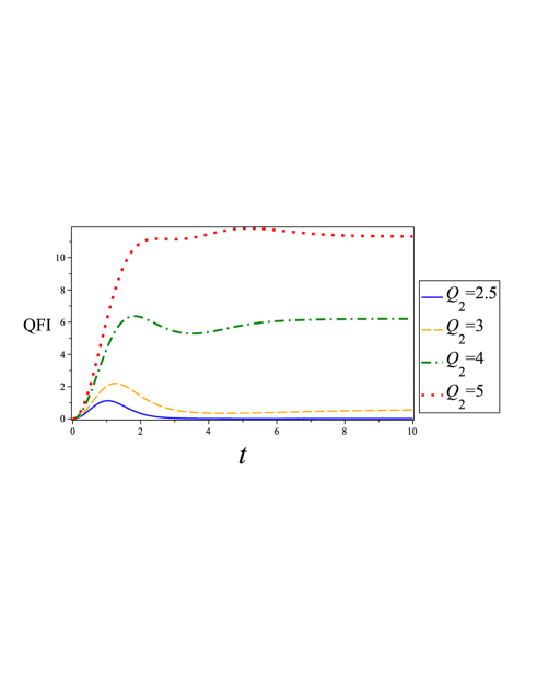
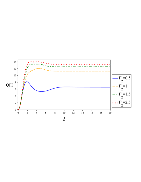
Figure 2: Dynamics of the quantum Fisher information (QFI) associated with $B_{1}$ as a function of (a) Ohmicity parameter $Q_{2}$ and (b) cutoff frequency $\Gamma_{2}$ controlled by Bob implementing the quantum sensing.

Because the quantum metrology process is implemented by Bob, it is reasonable to assume that we can control the environmental parameters at Bob’s location, while the same parameters at Alic’s location are out of our control. Therefore, we investigate how the remote sensing can be enhanced by controlling the interaction of working qubits in the process of the measurement.

The time variation of the QFI for different values of the Ohmicity parameter and cutoff frequency is plotted in Fig. 2. It shows that increasing the Ohmicity parameter $Q$ enhances the quantum estimation of the coupling strength and frustrates the QFI degradation (see Fig. 2). In fact, with increasing $Q$, after a while, the QFI becomes approximately constant over time, a phenomenon known as QFI trapping. Therefore, preparing a super-Ohmic environment at the location of the teleported qubits is the best strategy to extract information about the Alice’s coupling strength. The super-Ohmic environment frequently describes the effect of the interaction between a charged particle and its electromagnetic field. It should be noted that such engineering of the ohmicity of the spectrum can be implemented experimentally Haikka and Maniscalco (2014), e.g., when simulating the dephasing model in trapped ultracold atoms, as described in Ref. Haikka et al. (2011).

Figure 2 exhibits the important role of the cutoff frequency $\Gamma_{2}$, imposed on the Bob’s working qubits, in upgrading the sensors. Intensifying the cutoff frequency, Bob can retard the QFI loss and therefore enhance the remote sensing. Generally, the cutoff frequency $\Gamma_{2}$ is associated to a characteristic time $\tau_{c}\sim\Gamma_{2}^{-1}$ setting the fastest time scale of the irreversible dynamics. $\tau_{c}$ is usually known as the correlation time of the environment Benedetti et al. (2018); Salari Sehdaran et al. (2019). In our model, Bob can achieve the QFI trapping with imposing a high cutoff frequency.

Overall, in order to achieve the best efficiency in the process of remote sensing, Bob should effectively control the Ohmicity parameter as well as the cutoff frequency. In Ref. Jahromi and Haseli (2020), it has been discussed that how appropriate values of these parameters allow a transition from Markovian to non-Markovian qubit dynamics. Nevertheless, our results hold for both Markovian and non-Markovian evolution of the the two-qubit systems used as the teleportation resources.

Our numerical computation shows that intensifying the coupling strength $B_{2}$ causes the QFI to be suppressed, reducing the optimal precision of the estimation (see Fig. 3). Therefore, Bob should decrease the intensity of coupling strength in order to provide a proper condition for the quantum sensors. Tuning the coupling strengths is achievable in the experiments, by controlling the gate voltages of the tunneling junctions.

In Sec. IV.4, we investigate one of the physical origins of these phenomena.

IV.3 Feasible measurement for optimal estimation

Another important question is how we can physically design the optimal estimation, i.e., a practically feasible measurement whose Fisher information is equal to the QFI. Reminding that the optimal POVM can be constructed by the eigenvectors of the SLD, we should compute them and check whether these eigenvectors coincide with those of some observable of the system or not. Although in the general case this coincidence is not completely achievable, we interestingly find that with high cutoff frequency $\Gamma_{1}$ or large values of $Q_{1}$, the optimal POVM can be approximately constructed by the eigenvectors of $\sigma_{z}\otimes\sigma_{z}$. It means that measurement of $\sigma_{z}$ on each qubit leads to the near-optimal remote estimation, saturating the quantum upper bound.

IV.4 Quantum entanglement between teleported sensors

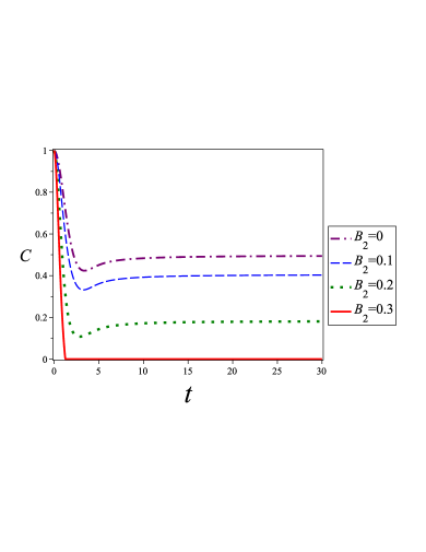
Figure 3: Time variation of entanglement, as quantified by concurrence $C(t)$, between the teleported qubits, playing the role of remote probes, for different values of the coupling strength $B_{2}$ controllable by Bob.

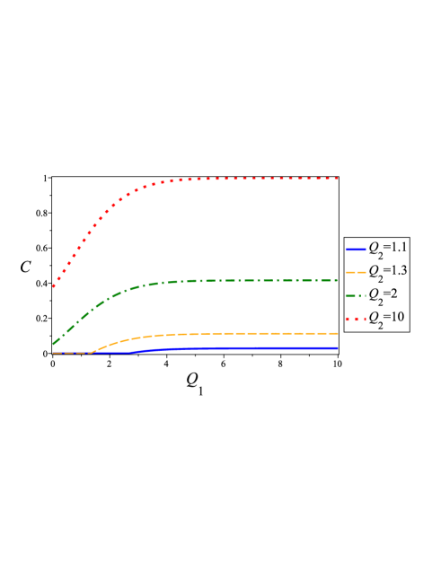
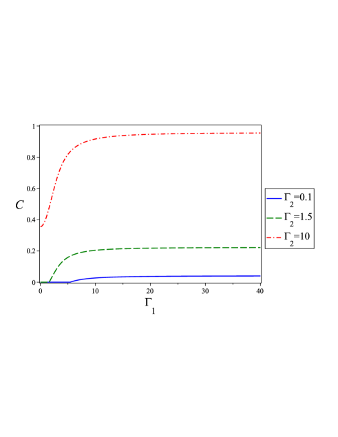
Figure 4: (a) Entanglement $C$ between remote sensors as a function of input Ohmicity parameter $Q_{1}$ for different values of the similar parameter $Q_{2}$ controlled by Bob. (b) The same quantity as a function of the input cutoff frequency $\Gamma_{1}$ for different values of $\Gamma_{2}$ denoting the cutoff frequency controlled by Bob.

It is known that quantum entanglement between localized qubits, used as quantum probes, may be a resource to achieve advantages in quantum metrology Giovannetti et al. (2011). Here we show that an increase in entanglement between the remote probes, realized by non-localized qubits, improves the quantum estimation.

Inserting Eq. (38) into Eq. (9), we find that the entanglement of the teleported qubits is give by

$$C(t)=2\max\left(0,\frac{1}{4}\left(2\alpha^{2}(t)\sin\theta\sin^{2}\vartheta-\left|\alpha^{4}(t)-1\right|\right)\right).$$ (61)

As seen in Fig. 3, an increase in the intensity of the coupling strength $B_{2}$, which can be controlled by Bob, decreases the entanglement between the sensors. It is one of the reasons leading to the decay of QFI with increasing $B_{2}$, because entanglement between the teleported qubits is an important resource helping Bob to effectively extract the information encoded into the sensors.

Moreover, entanglement may decrease abruptly and non-smoothly to zero in a finite time due to applying more strong coupling constant. Nevertheless, we find that the QFI is protected from this phenomenon called the sudden death. This shows that there are definitely other resources which can even compensate for the lack of the entanglement of the sensors in the process of remote sensing.

Because the sudden death of the entanglement may occur even when each of the qubits, used as the teleportation channel, interacts with a non-Markovian environment, we can introduce the non-Markovianty as another resource for the estimation. Nevertheless, protection of the QFI from sudden death in the presence of Markovian environments motivates more investigation of the resources playing significant roles in the remote sensing scenario.

Figure 4 illustrates the effects of the Ohmicity parameter $Q_{2}$ and cutoff frequency $\Gamma_{2}$, controlled by Bob implementing the quantum estimation, on the entanglement of the sensors and its sudden death.

At initial instants, increasing $Q_{2}~{}(Q_{1})$ can improve the entanglement and may decrease the critical value of $Q_{1}~{}(Q_{2})$ at which the sudden birth of the entanglement occurs. Therefore, an increase in $Q_{2}~{}(Q_{1})$ can remove the sudden death of the entanglement, appearing when decreasing $Q_{1}~{}(Q_{2})$ (see Fig. 4 plotted for $t=0.7$). It should be noted that these considerations are only of relevance to the early moments of the process. As time goes on such control is limited and Bob cannot completely counteract the sudden death of the entanglement by controlling his Ohmicity parameter.

Investigating the behavior of $C$ as a function of $\Gamma_{1}$ or $\Gamma_{2}$ for different values of $Q_{1}$ or $Q_{2}$, we obtain the similar results. Therefore, the Ohmicity parameters play an important role in controlling the entanglement of the quantum sensors and hence their sensitivity for detecting weak coupling coupling constants, because of the positive effect of the probe entanglement on the quantum estimation. In particular, we see that with large values of both $Q_{1}$ and $Q_{2}$ we can completely protect the initial maximal entanglement over time.

Similar control can be implemented by the cutoff frequency as illustrated in Fig. 4 plotted for $t=1.1$. In detail, studying the behavior of the entanglement between the remote probes as a function of $X\in\left\{Q_{1},Q_{2},\Gamma_{1}~{}(\Gamma_{2})\right\}$, we see that at initial instants an increase in the cutoff frequency $\Gamma_{2}~{}(\Gamma_{1})$ can improve the entanglement and may decrease the value of $X$ at which the sudden birth of the entanglement occurs. In other words, one can remove the sudden death of the entanglement, appearing with decreasing $X$, with an increase in the cutoff frequency. Again, as time goes on, such control is limited and we cannot completely counteract the sudden death of the entanglement by increasing $\Gamma_{2}~{}(\Gamma_{1})$.

IV.5 Near-perfect teleportation using non-local qubits

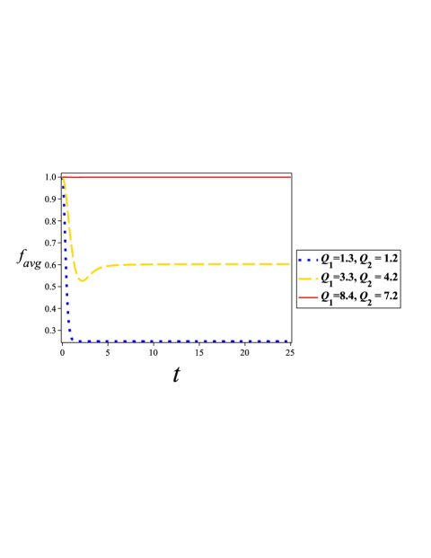
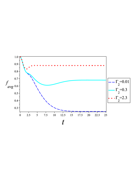
Figure 5: Dynamics of the average fidelity $f_{avg}$ of the teleportation for different values of (a) Ohmicity parameters $(Q_{1},Q_{2})$ and (b) cutoff frequency $\Gamma_{2}$ controlled by Bob performing the quantum sensing.

The quality of teleportation, i.e., closeness of the teleported state to the input state, can be specified by the fidelity Jozsa (1994) between input state $\rho_{\text{in}}=\ket{\psi_{in}}\bra{\psi_{in}}$ and output state $\rho_{\text{out}}$. Computing this measure, defined as $f\left(\rho_{\text{in}},\rho_{\text{out}}\right)=\left\{\text{Tr}\left[\sqrt{\left(\rho_{\text{in}}\right)^{\frac{1}{2}}\rho_{\text{out}}\left(\rho_{\text{in}}\right)^{\frac{1}{2}}}\right]\right\}^{2}=\langle\psi_{\text{in}}|\rho_{\text{out}}|\psi_{\text{in}}\rangle$. Moreover, the average fidelity, another notion for characterizing the quality of teleportation, is formulated as

$$f_{avg}=\frac{\int\limits_{0}^{2\pi}d\varphi\int\limits_{0}^{\pi}f\left(\rho_{\text{in}},\rho_{\text{out}}\right)\sin\theta~{}\text{d}\theta}{4\pi}.$$ (62)

In our model, we find that

$$f_{avg}=\frac{1}{12}\left(-2\alpha^{2}\cos 2\vartheta+3\alpha^{4}+4\alpha^{2}+3\right).$$ (63)

In classical communication maximum value of average fidelity is given by $2/3$ Popescu (1994). Therefore, implementing teleportation of a quantum state through a quantum resource, with fidelity larger than $2/3$ is worthwhile.

Figure 5 shows that how the average fidelity of the teleportation is affected by changing the Ohmicity parameters and cutoff frequency. When both Ohmicity parameters $Q_{1}$ and $Q_{2}$ increase, the average fidelity improves, as shown in Fig. 5. Interestingly, for large values of the Ohmicity parameters, we can even achieve the quasi-ideal teleportation with $f_{avg}\approx 1$. Therefore, non-local qubits interestingly allows us to realize near-perfect teleportation with mixed states in the presence of noises. We emphasize that, according to results presented in Jahromi and Haseli (2020), this near-perfect teleportation may occur for both Markovian and non-Markovian evolution.

Similar behaviour is observed in terms of $\Gamma_{2}$ (see Fig. 5). Bob can increase the quality of teleportation by an increase in his cutoff frequency $\Gamma_{2}$. In particular, imposing a high cutoff frequency, he can achieve average fidelity $f_{avg}>2/3$. Therefore, we can perform an efficient teleportation by controlling the cutoff frequency.

IV.6 Comparing output and channel resources with average fidelity as well as quantum Fisher information

Figure 6: Comparing the dynamics of the average fidelity as well as quantum Fisher information (QFI) with quantum resources (entanglement, quantum discord (QD), and quantum coherence) appearing in the teleportation channel state $\rho_{ch}$ and those emerging in the output state of the teleportation channel $\rho_{out}$.

It is known that the revivals of quantum correlations are associated with the non-Markovian evolution of the system Lo Franco et al. (2012). Moreover, the previous results Chanda and Bhattacharya (2016); He et al. (2017); Radhakrishnan et al. (2019); Wu et al. (2020) show that revivals of quantum coherence can be used for detecting non-Markovianity in incoherent operations naturally introduced as physical transformations that do not create coherence. It should be noted that the non-Markovianity, detected by BLP measure of non-Markovianity, discussed in Sec. III, is associated with the violation of P divisibility Rivas et al. (2010) and therefore of CP divisibility Breuer et al. (2009) while the non-Markovianity characterized by a coherence measure, based on a contractive distance, such as relative entropy Vedral (2002) or $l_{1}$-norm, corresponds to the violation of the CP divisibility.

Figure 6 illustrates the dynamics of quantum resources (quantum entanglement, quantum discord and quantum coherence) of the teleportation output state, those of the two-qubit system used as the teleportation channel, average fidelity of the teleportation, and the QFI. When the quantum discord and quantum coherence of the channel revive the non-Markovianity occurs, leading to appearance of the memory effects or backflow of information from the environment to the two-qubit system applied as the resource for the quantum teleportation. In the following, we explain the role of this non-Markovian effect to improve the teleportation.

Interestingly, we find that, in the absence of the entanglement sudden death, except for the QFI, all measures exhibit simultaneous oscillations with time such that their maximum and minimum points exactly coincide. This excellent agreement among the quantum resources of the channel, the average fidelity and the teleported quantum resources shows that the non-Markovianity of the channel and various quantum resources can be employed for enhancement of the average fidelity and hence faithfulness of the teleportation.

Figure 6 also shows that comparing the behavior of the QFI with other measures, we cannot faithfully detect the instant at which the optimal estimation is achieved. Nevertheless, the time when the QFI is minimized and hence we should avoid it in the process of estimation, can be detected by inspecting the minimum points of the quantum resources.

V Conclusions

Efficient quantum communication among qubits relies on robust networks, which allow for fast and coherent transfer of quantum information. In this paper we have investigated faithful teleportation of quantum states as well as quantum correlations by non-local topological qubits realized by Majorana modes and independently coupled to non-Markovian Ohmic-like reservoirs. The roles of control parameters to enhance the teleportation have been discussed in detail. In Ref. Laine et al. (2014) the authors showed that nonlocal memory effects can substantially increase the fidelity of mixed state quantum teleportation in the presence of dephasing noise such that perfect quantum teleportation can be achieved even with mixed photon polarisation states. In their protocol, the nonlocal memory effects occur due to initial correlations between the local environments of the photons. Here we have illustrated that using non-local topological qubits, one can perform near-perfect mixed state teleportation, even in the absence of non-Markovianty and memory effects.

We have also designed a scheme for remote sensing through the teleported qubits for estimating some parameter at Alice’s location. Without loss of generality, Bob intends to estimate the strength of coupling between Alice’s qubits, used as the teleportation resource, and their environments. It has been shown that the quantum estimation can be considerably enhanced by controlling the environmental parameters whether the evolution is Markovain or non-Markovianity.

Another important issue which should be addressed is why before the teleportation Bob does not employ his qubits, entangled with Alice’s qubits, to estimate $B_{1}$. The reason is that by performing local operations, Bob definitely changes the state of the resource channel and hence it may be unusable for quantum information tasks requiring entanglement such as quantum teleportation, quantum key distribution, etc. Moreover, these changes as well as Bob’s activities to estimate some parameter in Alice’s location can be detectable by her, while he might want to do it secretly.

In detail, performing a quantum information task involving communication between Alice and Bob, the two parties should consider two important security conditions Zhu et al. (2006); Li et al. (2006); Chou et al. (2018, 2021): security against internal and external attacks. In internal attacks, either Alice or Bob attempts to steal the other’s secret information. However, in external attacks an eavesdropper, Eve, attempts to steal messages without being detected by Alice or Bob. Because of these security considerations, always performing security checks by Alice and Bob is always necessary to detect internal or external attacks. Bob’s activities to estimate one of Alice’s parameters through the qubits used for the resource channel can be detected by Alice in the security check. Therefore, Bob prefers to hide his activities from Alice and employ teleported qubits for implementing the remote sensing.

Recently, a quantum simulation of the teleportation of a qubit encoded as the Majorana zero mode states of the Kitaev chain has been performed Huang et al. (2021). Our work motivates further studies on physical realization of quantum teleportation by large number of non-local topological qubits and paves the way for designing remote sensors based on Majorana modes.

Declaration of competing interest

We have no competing interests.

References

- Wootters and Zurek (1982) William K Wootters and Wojciech H Zurek, “A single quantum cannot be cloned,” Nature 299, 802–803 (1982).
- Bennett et al. (1993) Charles H Bennett, Gilles Brassard, Claude Crépeau, Richard Jozsa, Asher Peres, and William K Wootters, “Teleporting an unknown quantum state via dual classical and einstein-podolsky-rosen channels,” Phys. Rev. Lett. 70, 1895 (1993).
- Raussendorf and Briegel (2001) Robert Raussendorf and Hans J Briegel, “A one-way quantum computer,” Phys. Rev. Lett. 86, 5188 (2001).
- Sangouard et al. (2011) Nicolas Sangouard, Christoph Simon, Hugues De Riedmatten, and Nicolas Gisin, “Quantum repeaters based on atomic ensembles and linear optics,” Rev. Mod. Phys. 83, 33 (2011).
- Gottesman and Chuang (1999) Daniel Gottesman and Isaac L Chuang, “Demonstrating the viability of universal quantum computation using teleportation and single-qubit operations,” Nature 402, 390–393 (1999).
- Bouwmeester et al. (1997) Dik Bouwmeester, Jian-Wei Pan, Klaus Mattle, Manfred Eibl, Harald Weinfurter, and Anton Zeilinger, “Experimental quantum teleportation,” Nature 390, 575–579 (1997).
- Riebe et al. (2004) Mark Riebe, H Häffner, CF Roos, W Hänsel, J Benhelm, GPT Lancaster, TW Körber, C Becher, F Schmidt-Kaler, DFV James, et al., “Deterministic quantum teleportation with atoms,” Nature 429, 734–737 (2004).
- Barrett et al. (2004) MD Barrett, J Chiaverini, T Schaetz, J Britton, WM Itano, JD Jost, E Knill, C Langer, D Leibfried, R Ozeri, et al., “Deterministic quantum teleportation of atomic qubits,” Nature 429, 737–739 (2004).
- Sherson et al. (2006) Jacob F Sherson, Hanna Krauter, Rasmus K Olsson, Brian Julsgaard, Klemens Hammerer, Ignacio Cirac, and Eugene S Polzik, “Quantum teleportation between light and matter,” Nature 443, 557–560 (2006).
- Hou et al. (2016) P-Y Hou, Y-Y Huang, X-X Yuan, X-Y Chang, Chong Zu, Li He, and L-M Duan, “Quantum teleportation from light beams to vibrational states of a macroscopic diamond,” Nat. Commun. 7, 1–7 (2016).
- Pirandola et al. (2015) Stefano Pirandola, Jens Eisert, Christian Weedbrook, Akira Furusawa, and Samuel L Braunstein, “Advances in quantum teleportation,” Nat. Photonics 9, 641–652 (2015).
- Kumar et al. (2020) Abhijeet Kumar, Saeed Haddadi, Mohammad Reza Pourkarimi, Bikash K Behera, and Prasanta K Panigrahi, “Experimental realization of controlled quantum teleportation of arbitrary qubit states via cluster states,” Sci. Rep. 10, 1–16 (2020).
- Liu et al. (2020) Zhao-Di Liu, Yong-Nan Sun, Bi-Heng Liu, Chuan-Feng Li, Guang-Can Guo, Sina Hamedani Raja, Henri Lyyra, and Jyrki Piilo, “Experimental realization of high-fidelity teleportation via a non-markovian open quantum system,” Phys. Rev. A 102, 062208 (2020).
- Langenfeld et al. (2021) Stefan Langenfeld, Stephan Welte, Lukas Hartung, Severin Daiss, Philip Thomas, Olivier Morin, Emanuele Distante, and Gerhard Rempe, “Quantum teleportation between remote qubit memories with only a single photon as a resource,” Phys. Rev. Lett. 126, 130502 (2021).
- Holevo (1978) AS Holevo, “Estimation of shift parameters of a quantum state,” Rep. Math. Phys. 13, 379–399 (1978).
- Giovannetti et al. (2004) Vittorio Giovannetti, Seth Lloyd, and Lorenzo Maccone, “Quantum-enhanced measurements: Beating the standard quantum limit,” Science 306, 1330 (2004).
- Paris (2009) Matteo GA Paris, “Quantum estimation for quantum technology,” Int. J. Quantum Inf. 7, 125–137 (2009).
- Giovannetti et al. (2011) Vittorio Giovannetti, Seth Lloyd, and Lorenzo Maccone, “Advances in quantum metrology,” Nat. Photonics 5, 222–229 (2011).
- Liu et al. (2019) Jing Liu, Haidong Yuan, Xiao-Ming Lu, and Xiaoguang Wang, “Quantum fisher information matrix and multiparameter estimation,” J. Phys. A 53, 023001 (2019).
- Tóth and Apellaniz (2014) Géza Tóth and Iagoba Apellaniz, “Quantum metrology from a quantum information science perspective,” J. Phys. A 47, 424006 (2014).
- Polino et al. (2020) Emanuele Polino, Mauro Valeri, Nicolò Spagnolo, and Fabio Sciarrino, “Photonic quantum metrology,” AVS Quantum Science 2, 024703 (2020).
- Pirandola et al. (2018) S. Pirandola, B. Roy Bardhan, T. Gehring, C. Weedbrook, and S. Lloyd, “Advances in photonic quantum sensing,” Nat. Photon. 12, 724 (2018).
- Bongs et al. (2019) K. Bongs, M. Holynski, J. Vovrosh, P. Bouyer, G. Condon, E. Rasel, C. Schubert, W. P. Schleich, and A. Roura, “Taking atom interferometric quantum sensors from the laboratory to real-world applications,” Nat. Rev. Phys. 1, 731 (2019).
- Pezzè et al. (2018) Luca Pezzè, Augusto Smerzi, Markus K. Oberthaler, Roman Schmied, and Philipp Treutlein, “Quantum metrology with nonclassical states of atomic ensembles,” Rev. Mod. Phys. 90, 035005 (2018).
- Vijay and Fu (2016) Sagar Vijay and Liang Fu, “Teleportation-based quantum information processing with majorana zero modes,” Phys. Rev. B 94, 235446 (2016).
- Brask et al. (2015) Jonatan Bohr Brask, Rafael Chaves, and Jan Kołodyński, “Improved quantum magnetometry beyond the standard quantum limit,” Phys. Rev. X 5, 031010 (2015).
- Wang et al. (2018) Kunkun Wang, Xiaoping Wang, Xiang Zhan, Zhihao Bian, Jian Li, Barry C Sanders, and Peng Xue, “Entanglement-enhanced quantum metrology in a noisy environment,” Phys. Rev. A 97, 042112 (2018).
- Braun et al. (2018) Daniel Braun, Gerardo Adesso, Fabio Benatti, Roberto Floreanini, Ugo Marzolino, Morgan W Mitchell, and Stefano Pirandola, “Quantum-enhanced measurements without entanglement,” Rev. Mod. Phys. 90, 035006 (2018).
- Liu et al. (2021) Li-Zheng Liu, Yu-Zhe Zhang, Zheng-Da Li, Rui Zhang, Xu-Fei Yin, Yue-Yang Fei, Li Li, Nai-Le Liu, Feihu Xu, Yu-Ao Chen, et al., “Distributed quantum phase estimation with entangled photons,” Nat. Photonics 15, 137–142 (2021).
- Rangani Jahromi (2020) H. Rangani Jahromi, “Quantum thermometry in a squeezed thermal bath,” Phys. Scr. 95, 035107 (2020).
- Rangani Jahromi (2019) H Rangani Jahromi, “Weak measurement effect on optimal estimation with lower and upper bound on relativistic metrology,” Int. J. Mod. Phys. D 28, 1950162 (2019).
- Hu et al. (1992) Bei Lok Hu, Juan Pablo Paz, and Yuhong Zhang, “Quantum brownian motion in a general environment: Exact master equation with nonlocal dissipation and colored noise,” Phys. Rev. D 45, 2843 (1992).
- Boyanovsky et al. (2005) D Boyanovsky, K Davey, and Chiu Man Ho, “Particle abundance in a thermal plasma: Quantum kinetics versus boltzmann equation,” Phys.Rev. D 71, 023523 (2005).
- Ho et al. (2014) Shih-Hao Ho, Sung-Po Chao, Chung-Hsien Chou, and Feng-Li Lin, “Decoherence patterns of topological qubits from majorana modes,” New J. Phys. 16, 113062 (2014).
- Liu et al. (2013) Hai-Bin Liu, Jun-Hong An, Chong Chen, Qing-Jun Tong, Hong-Gang Luo, and CH Oh, “Anomalous decoherence in a dissipative two-level system,” Phys. Rev. A 87, 052139 (2013).
- Wu (2014) Shin-Tza Wu, “Quenched decoherence in qubit dynamics due to strong amplitude-damping noise,” Phys. Rev. A 89, 034301 (2014).
- Invernizzi et al. (2008) Carmen Invernizzi, Michael Korbman, Lorenzo Campos Venuti, and Matteo GA Paris, “Optimal quantum estimation in spin systems at criticality,” Phys. Rev. A 78, 042106 (2008).
- Freedman et al. (2003) Michael Freedman, Alexei Kitaev, Michael Larsen, and Zhenghan Wang, “Topological quantum computation,” Bull. Am. Math. Soc 40, 31–38 (2003).
- Nayak et al. (2008) Chetan Nayak, Steven H Simon, Ady Stern, Michael Freedman, and Sankar Das Sarma, “Non-abelian anyons and topological quantum computation,” Rev. Mod. Phys. 80, 1083 (2008).
- Fu and Kane (2008) Liang Fu and Charles L Kane, “Superconducting proximity effect and majorana fermions at the surface of a topological insulator,” Phys. Rev. Lett. 100, 096407 (2008).
- Hasan and Kane (2010) M Zahid Hasan and Charles L Kane, “Colloquium: topological insulators,” Rev. Mod. Phys. 82, 3045 (2010).
- Qi and Zhang (2011) Xiao-Liang Qi and Shou-Cheng Zhang, “Topological insulators and superconductors,” Rev. Mod. Phys. 83, 1057 (2011).
- Wilczek (2009) Frank Wilczek, “Majorana returns,” Nat. Phys. 5, 614–618 (2009).
- Arovas et al. (1984) Daniel Arovas, John R Schrieffer, and Frank Wilczek, “Fractional statistics and the quantum hall effect,” Phys. Rev. Lett. 53, 722 (1984).
- Ivanov (2001) Dmitri A Ivanov, “Non-abelian statistics of half-quantum vortices in p-wave superconductors,” Phys. Rev. Lett. 86, 268 (2001).
- Kitaev (2001) A Yu Kitaev, “Unpaired majorana fermions in quantum wires,” Phys.-Uspekhi 44, 131 (2001).
- Sau et al. (2010) Jay D Sau, Roman M Lutchyn, Sumanta Tewari, and S Das Sarma, “Generic new platform for topological quantum computation using semiconductor heterostructures,” Phys. Rev. Lett. 104, 040502 (2010).
- Alicea (2010) Jason Alicea, “Majorana fermions in a tunable semiconductor device,” Phys. Rev. B 81, 125318 (2010).
- Thakurathi et al. (2014) Manisha Thakurathi, K Sengupta, and Diptiman Sen, “Majorana edge modes in the kitaev model,” Phys. Rev. B 89, 235434 (2014).
- Rivas et al. (2014) Ángel Rivas, Susana F Huelga, and Martin B Plenio, “Quantum non-markovianity: characterization, quantification and detection,” Rep. Prog. Phys. 77, 094001 (2014).
- Breuer (2012) Heinz-Peter Breuer, “Foundations and measures of quantum non-markovianity,” J. Phys. B 45, 154001 (2012).
- Li et al. (2018) Li Li, Michael JW Hall, and Howard M Wiseman, “Concepts of quantum non-markovianity: A hierarchy,” Phys. Rep. 759, 1–51 (2018).
- Bowen and Bose (2001) Garry Bowen and Sougato Bose, “Teleportation as a depolarizing quantum channel, relative entropy, and classical capacity,” Phys. Rev. Lett. 87, 267901 (2001).
- Lee and Kim (2000a) Jinhyoung Lee and MS Kim, “Entanglement teleportation via werner states,” Phys. Rev. Lett. 84, 4236 (2000a).
- Helstrom (1969) Carl W Helstrom, “Quantum detection and estimation theory,” Journal of Statistical Physics 1, 231–252 (1969).
- Braunstein et al. (1996) Samuel L Braunstein, Carlton M Caves, and Gerard J Milburn, “Generalized uncertainty relations: theory, examples, and lorentz invariance,” Ann. Phys. 247, 135–173 (1996).
- Jing et al. (2014) Liu Jing, Jing Xiao-Xing, Zhong Wei, and Wang Xiao-Guang, “Quantum fisher information for density matrices with arbitrary ranks,” Commun. Theor. Phys. 61, 45 (2014).
- Liu et al. (2016) Jing Liu, Jie Chen, Xiao-Xing Jing, and Xiaoguang Wang, “Quantum fisher information and symmetric logarithmic derivative via anti-commutators,” J. Phys. A 49, 275302 (2016).
- Wootters (1998) William K Wootters, “Entanglement of formation of an arbitrary state of two qubits,” Phys. Rev. Lett. 80, 2245 (1998).
- Bennett et al. (1996) Charles H Bennett, David P DiVincenzo, John A Smolin, and William K Wootters, “Mixed-state entanglement and quantum error correction,” Phys. Rev. A 54, 3824 (1996).
- Streltsov et al. (2017) Alexander Streltsov, Gerardo Adesso, and Martin B Plenio, “Colloquium: Quantum coherence as a resource,” Rev. Mod. Phys. 89, 041003 (2017).
- Shao et al. (2015) Lian-He Shao, Zhengjun Xi, Heng Fan, and Yongming Li, “Fidelity and trace-norm distances for quantifying coherence,” Phys. Rev. A 91, 042120 (2015).
- Baumgratz et al. (2014) Tillmann Baumgratz, Marcus Cramer, and Martin B Plenio, “Quantifying coherence,” Phys. Rev. Lett. 113, 140401 (2014).
- Yao et al. (2015) Yao Yao, Xing Xiao, Li Ge, and CP Sun, “Quantum coherence in multipartite systems,” Phys. Rev. A 92, 022112 (2015).
- Ollivier and Zurek (2001) Harold Ollivier and Wojciech H Zurek, “Quantum discord: a measure of the quantumness of correlations,” Phys. Rev. Lett. 88, 017901 (2001).
- Fanchini et al. (2017) Felipe Fernandes Fanchini, Diogo de Oliveira Soares Pinto, and Gerardo Adesso, Lectures on General Quantum Correlations and Their Applications (Springer, 2017).
- Pirandola (2014) Stefano Pirandola, “Quantum discord as a resource for quantum cryptography,” Sci. Rep. 4, 1–5 (2014).
- Wang et al. (2010) Cheng-Zhi Wang, Chun-Xian Li, Liu-Ying Nie, and Jiang-Fan Li, “Classical correlation and quantum discord mediated by cavity in two coupled qubits,” J. Phys. B 44, 015503 (2010).
- Gessner and Smerzi (2018) Manuel Gessner and Augusto Smerzi, “Statistical speed of quantum states: Generalized quantum Fisher information and Schatten speed,” Phys. Rev. A 97, 022109 (2018).
- Luo and Zhang (2004) Shunlong Luo and Qiang Zhang, “Informational distance on quantum-state space,” Phys. Rev. A 69, 032106 (2004).
- Ozawa (2000) Masanao Ozawa, “Entanglement measures and the Hilbert-Schmidt distance,” Phys. Lett. A 268, 158–160 (2000).
- Chao et al. (2013) Sung-Po Chao, Salman A Silotri, and Chung-Hou Chung, “Nonequilibrium transport of helical luttinger liquids through a quantum dot,” Phys. Rev. B 88, 085109 (2013).
- Breuer et al. (2009) Heinz-Peter Breuer, Elsi-Mari Laine, and Jyrki Piilo, “Measure for the degree of non-markovian behavior of quantum processes in open systems,” Phys. Rev. Lett. 103, 210401 (2009).
- Jahromi and Haseli (2020) H Rangani Jahromi and S Haseli, “Quantum memory and quantum correlations of majorana qubits used for magnetometry,” Quantum Inf. Comput. 2 20, 0935 (2020).
- Jahromi et al. (2020) Hossein Rangani Jahromi, Kobra Mahdavipour, Mahshid Khazaei Shadfar, and Rosario Lo Franco, “Witnessing non-markovian effects of quantum processes through hilbert-schmidt speed,” Phys. Rev. A 102, 022221 (2020).
- Leung (2003) Debbie W Leung, “Choi’s proof as a recipe for quantum process tomography,” J. Math. Phys. 44, 528–533 (2003).
- Jahromi and Franco (2021) Hossein Rangani Jahromi and Rosario Lo Franco, “Hilbert–schmidt speed as an efficient figure of merit for quantum estimation of phase encoded into the initial state of open n-qubit systems,” Sci. Rep. 11, 1–16 (2021).
- Nielsen and Chuang (2002) Michael A Nielsen and Isaac Chuang, “Quantum computation and quantum information,” (2002).
- Lee and Kim (2000b) Jinhyoung Lee and M. S. Kim, “Entanglement teleportation via werner states,” Phys. Rev. Lett. 84, 4236–4239 (2000b).
- Haikka and Maniscalco (2014) Pinja Haikka and Sabrina Maniscalco, “Non-markovian quantum probes,” Open Syst. Inf. Dyn 21, 1440005 (2014).
- Haikka et al. (2011) Pinja Haikka, Suzanne McEndoo, Gabriele De Chiara, GM Palma, and Sabrina Maniscalco, “Quantifying, characterizing, and controlling information flow in ultracold atomic gases,” Phys. Rev. A 84, 031602 (2011).
- Benedetti et al. (2018) Claudia Benedetti, Fahimeh Salari Sehdaran, Mohammad H Zandi, and Matteo GA Paris, “Quantum probes for the cutoff frequency of ohmic environments,” Phys. Rev. A 97, 012126 (2018).
- Salari Sehdaran et al. (2019) Fahimeh Salari Sehdaran, Matteo Bina, Claudia Benedetti, and Matteo GA Paris, “Quantum probes for ohmic environments at thermal equilibrium,” Entropy 21, 486 (2019).
- Jozsa (1994) Richard Jozsa, “Fidelity for mixed quantum states,” J. Mod. Opt. 41, 2315–2323 (1994).
- Popescu (1994) Sandu Popescu, “Bell’s inequalities versus teleportation: What is nonlocality?” Phys. Rev. Lett. 72, 797 (1994).
- Lo Franco et al. (2012) R. Lo Franco, B. Bellomo, E. Andersson, and G. Compagno, “Revival of quantum correlations without system-environment back-action,” Phys. Rev. A 85, 032318 (2012).
- Chanda and Bhattacharya (2016) Titas Chanda and Samyadeb Bhattacharya, “Delineating incoherent non-markovian dynamics using quantum coherence,” Ann. Phys. 366, 1–12 (2016).
- He et al. (2017) Zhi He, Hao-Sheng Zeng, Yan Li, Qiong Wang, and Chunmei Yao, “Non-markovianity measure based on the relative entropy of coherence in an extended space,” Phys. Rev. A 96, 022106 (2017).
- Radhakrishnan et al. (2019) Chandrashekar Radhakrishnan, Po-Wen Chen, Segar Jambulingam, Tim Byrnes, and Md Manirul Ali, “Time dynamics of quantum coherence and monogamy in a non-markovian environment,” Sci. Rep. 9, 1–10 (2019).
- Wu et al. (2020) Kang-Da Wu, Zhibo Hou, Guo-Yong Xiang, Chuan-Feng Li, Guang-Can Guo, Daoyi Dong, and Franco Nori, “Detecting non-markovianity via quantified coherence: theory and experiments,” npj Quantum Inf. 6, 1–7 (2020).
- Rivas et al. (2010) Ángel Rivas, Susana F Huelga, and Martin B Plenio, “Entanglement and non-markovianity of quantum evolutions,” Phys. Rev. Lett. 105, 050403 (2010).
- Vedral (2002) Vlatko Vedral, “The role of relative entropy in quantum information theory,” Rev. Mod. Phys. 74, 197 (2002).
- Laine et al. (2014) Elsi-Mari Laine, Heinz-Peter Breuer, and Jyrki Piilo, “Nonlocal memory effects allow perfect teleportation with mixed states,” Sci. Rep. 4, 1–5 (2014).
- Zhu et al. (2006) Ai-Dong Zhu, Yan Xia, Qiu-Bo Fan, and Shou Zhang, “Secure direct communication based on secret transmitting order of particles,” Phys. Rev. A 73, 022338 (2006).
- Li et al. (2006) Xi-Han Li, Fu-Guo Deng, and Hong-Yu Zhou, “Improving the security of secure direct communication based on the secret transmitting order of particles,” Phys. Rev. A 74, 054302 (2006).
- Chou et al. (2018) Yao-Hsin Chou, Guo-Jyun Zeng, Zhe-Hua Chang, and Shu-Yu Kuo, “Dynamic group multi-party quantum key agreement,” Sci. Rep. 8, 1–13 (2018).
- Chou et al. (2021) Yao-Hsin Chou, Guo-Jyun Zeng, Xing-Yu Chen, and Shu-Yu Kuo, “Multiparty weighted threshold quantum secret sharing based on the chinese remainder theorem to share quantum information,” Sci. Rep. 11, 1–10 (2021).
- Huang et al. (2021) He-Liang Huang, Marek Narożniak, Futian Liang, Youwei Zhao, Anthony D Castellano, Ming Gong, Yulin Wu, Shiyu Wang, Jin Lin, Yu Xu, et al., “Emulating quantum teleportation of a majorana zero mode qubit,” Phys. Rev. Lett. 126, 090502 (2021).