RVMDE: Radar Validated Monocular Depth Estimation for Robotics

Abstract

Stereoscopy demonstrates a natural perception of distance in a scene, and its manifestation in the perception of the 3D world is an involuntary phenomenon. However, an innate rigid calibration of binocular vision sensors is crucial for accurate depth estimation. Alternatively, a monocular camera alleviates the limitation at the expense of accuracy in estimating depth, and the challenges aggravate difficult imaging conditions. Moreover, an optical sensor often fails to acquire vital signals in rough environments, and radar is used instead, which gives coarse but more accurate signals. This work explores the utility of coarse signals from radar when fused with fine-grained data from a monocular camera for depth estimation in various environmental conditions. Furthermore, a variant of the feature pyramid network (FPN) is proposed which extensively operates on fine-grained image features at multiple scales with a fewer number of parameters. The FPN processes image feature maps are fused with radar data features extracted with a convolutional neural network. The concatenated hierarchical features are used to predict the depth with ordinal regression. We performed experiments on the nuScenes dataset, and the proposed architecture stays on top in quantitative evaluations with reduced parameters and faster inference. The depth estimation results suggest that the proposed techniques can be used as an alternative to stereo depth estimation in critical applications in robotics and self-driving cars.

I Introduction

Robots mobility among humans is an imminent technology wonder. Although pre-programmed robots have been an integral part of industries, autonomous robots have yet to leave the labs. The apprehended applications of autonomous robots are growing with every passing moment in all services, i.e., healthcare, surveillance, transportation, education, and hospitality. A desideratum of robots’ integration into humans’ social systems is their seamless behavior. Robots develop cognition based on a perception of an operating environment and use sensors to perceive data from the surroundings.

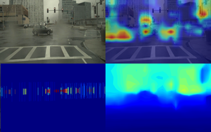
Figure 1: First column (top to bottom) depicts a selected test image and corresponding radar markers with extended height. Second column (top to bottom) shows the class activation maps and the estimated depth using the proposed methodology.

Standard sensors, like cameras, radar, lidar, and ultrasonic sensors, usually translate signals into comprehensible and interpretable information. The advancements in computer vision make cameras ubiquitous sensors, and it equips robots with an animate view of surroundings only after processing the captured images using AI algorithms. Essential information for mobility is a perception of the 3D environment that includes distances and depth calculations. Humans rely on stereoscopic vision, and a stereo camera imitates the function with rigid calibration of the sensors. A limitation of stereo camera vision is its rigid calibration, thus limiting its utility in diverse applications. Lidar is an alternative optical sensor that retrieves more accurate depth information with fewer limitations, but it is an expensive sensor to date. A monocular camera depth estimation is another cheap alternative for distance perception.

Monocular depth estimation is an ill-posed problem as a single view does not provide sufficient data to generate depth that complies with geometrical constraints. Instead, estimation techniques are adopted to generate depth information relevant to the visual cues present in an image. Radar is another ubiquitous sensor, and its signals can help to generate depth-validated visual cues. This study explores radar validated monocular depth estimation (RVMDE) that fuses radar data with image data and predicts distance values. Fig. 1 depicts the class activation maps of the validated depth cues with additional radar markers. Monocular depth estimation is a regression problem, and deep neural networks (DNN) are widely used to predict depth only with images. Variants of convolutional neural network (CNN), which perform in classification, detection, and segmentation tasks, are employed in the depth estimation task. Radar data fused with RGB image data is explored with various compositions of DNN and various data fusion strategies. RVMDE proposed a CNN composition which is a variant of a feature pyramid network (FPN). It explores image features at multiple scales and learns to fuse the image features associated with radar markers filtered with convolutional layers. Depth computation is often formulated as a per-pixel regression task. However, the perspective projection accommodates the mapping of the regression task to a classification task where the distance is divided into ordered groups. RVMDE evaluation employs the ordinal regression technique [7] to estimate the depth of the study which helped us to evaluate the effects of data validation using class activation maps (CAM).

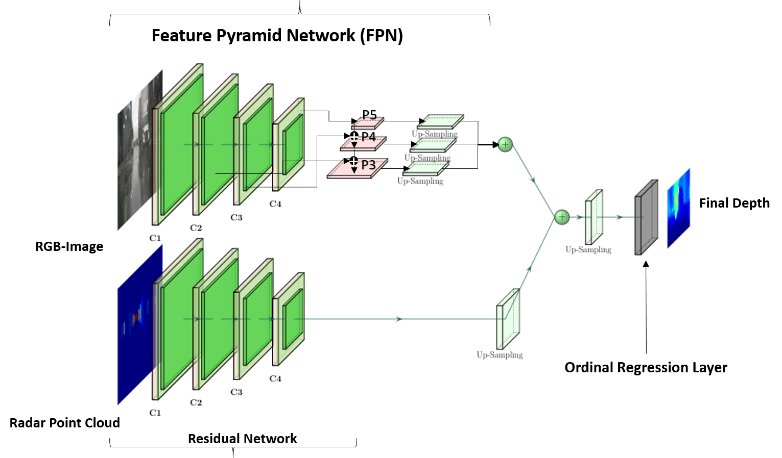
Figure 2: An overview of proposed models structure. Late-fusion technique is applied to extracted features from both the binocular modalities. At the end an ordinal regression layers is applied for Monocular depth estimation.

Since radar data is sparse and provides coarser data than the RGB image data, it is often fused with RGB with a late fusion technique. The late fusion encodes the RGB data to a lower modality and concatenates with sparse radar data. In this study, we experiment with early, mid and late data fusion techniques and empirically suggest the use of late data fusion. Another intervention to improve the coarse data markers generated by radar is to extend the available markers corresponding to the RGB image data. Earlier, heuristic-based marker extension techniques were used in object detection [9] and later used for depth estimation [2]. RVMDE uses the CNN network to encode the heuristically extended radar marker and fuse the encoded radar data later with encoded RGB image data. A recent sophisticated marker extension technique associates the RGB pixel information with radar marker and generates a fine-grained extension of radar data [16]. In this work, we test our proposed composition of DNN for monocular depth estimation with the fine-grained extension of radar data.

Robotics and its applications stipulate cost-effective and robust solutions of the challenges. We address the depth perception in 3D world understanding using a monocular camera and a radar in this study. The late fusion technique concatenates hierarchical FPN for images and standard deep CNN for radar data. We adopt ordinal regression loss for training and extend the sparse radar data with fine-grained markers and shows the value added by the radar data and image pyramid features using CAM. The composition of our manuscript is as follows: In section-II, we present the related work, and section-III is comprised of the proposed methodology. In section-IV, the experimental work and results are explained, section-V, V-B the ablation study and extended work and at the end section-VI briefs the conclusion.

II Related Work

This section limits the discussion to recent advancements in monocular depth estimation standalone and with data fusion. For interested readers, literature on monocular depth, estimation is detailed in [28], [29], [39],[40],[41].

II-A Monocular Depth Estimation

For robotics and self-driving, depth estimation using images is cost-effective, and it beseems the advances in computer vision research. Earlier, depth estimation for 3D world understanding used stereo images with DNN [18], [28], [29]. However, stereo images limit the applications, thus demanding cheaper, robust, and simple monocular depth estimation. As depth estimation with a single camera is an ill-posed problem, in the absence of labeled datasets, earlier pattern recognition solutions suggest handcrafted features extraction for monocular depth estimation[19],[20]. Later, advances in deep learning and availability of labeled datasets [21],[22] inspired the use of celebrated CNN for the depth prediction [23, 24]. A series of CNN inspired works on depth estimation using monocular images demonstrated the idea worthy of use in robotics challenging environment [3],[4],[7],[25],[34],[35],[36]. Namely, dense representation [26] achieved using skip-connections generates the multi-scale feature maps and uses it for the depth prediction using common $L1$ loss [32]. [3], introduced a DNN with ordinal regression loss, which transforms the regression to spacing increased discretization (SID) and changed the regression to a classification task.

II-B Validation using Radars Markers

Although monocular depth estimation is a viable solution, it does not inherit depth cues and suffers in challenging environmental conditions. Radar provides precise depth information, and it is a cost-effective and standard sensor in robotics suite. Data fusion of images with additional accurate depth information from radar markers validates visual features and improves depth estimation. Recently, [15], [9] employed a deep learning-based approach for object detection using radar’s point cloud data as an extra channel with monocular images. Their work motivated our study to utilize radar as an additional sensor for depth estimation in challenging scenarios.

[2] exploits the use of different fusion methods of RGB and radar data for depth estimation and tested encoder-decoder architecture with a CNN model to show early fusion, mid fusion, late fusion, and multi-level fusion results. Based on their findings, late fusion and multi-layer techniques suit the sparsity of radar data. [17] proposed a solution with RGB and rada data fusion which extracts the features from both modalities using a region proposal network (RPN) and detection heads and generates point cloud data-guided region of interest (ROI). A deep ordinal regression network (DORN) is adopted for monocular depth estimation with radar data in [5] with the limited field of view and early and late fusion approaches. The radar data is augmented by extended data markers using a heuristic approach, and the augmentation showed improved results in diverse weather conditions. Most of the radar-camera fusion strategies focus on fusion at the detection stage, whereas [16] uses a pixel-level fusion of data. The fusion poses mapping issues which they resolve with two-stage architectures. The first stage associates radar depth and image pixel and converts the data to multi-channel enhance radar (MER) data, which is fed to another DNN for depth completion in the second stage. In another study, the author uses a self-supervised approach for depth estimation tasks with radar data as a weak supervision signal at training time [6]. Radar data is optional for inference to overcome the inherent noise and data sparsity issues of radar.

III Proposed Methodology

The proposed methodology comprises three modules: a modified feature pyramid network (FPN), a standard CNN, and an ordinal regression layer as shown in Fig. 2. Each of these modules is explained in the coming subsections. Briefly, the RGB image data is passed to a modified FPN [13] with ResNet as a backbone [11] and the radar data is passed to ResNet CNN. The features of RGB image and radar data are concatenated, up-sampled, and passed to the ordinal regression layer [7]. The camera image is fine-grained data, whereas radar generates coarser markers of detection. The radar markers are extended in height [9] heuristically, which is used as an input for feature detection and validating depth information in images. Furthermore, a sophisticated heuristic of using multiple channels marking color with increasing depth was considered [16], which was later abandoned in favor of an intelligent pixel to depth association method for representing radar data. The details of the modules are as follows:

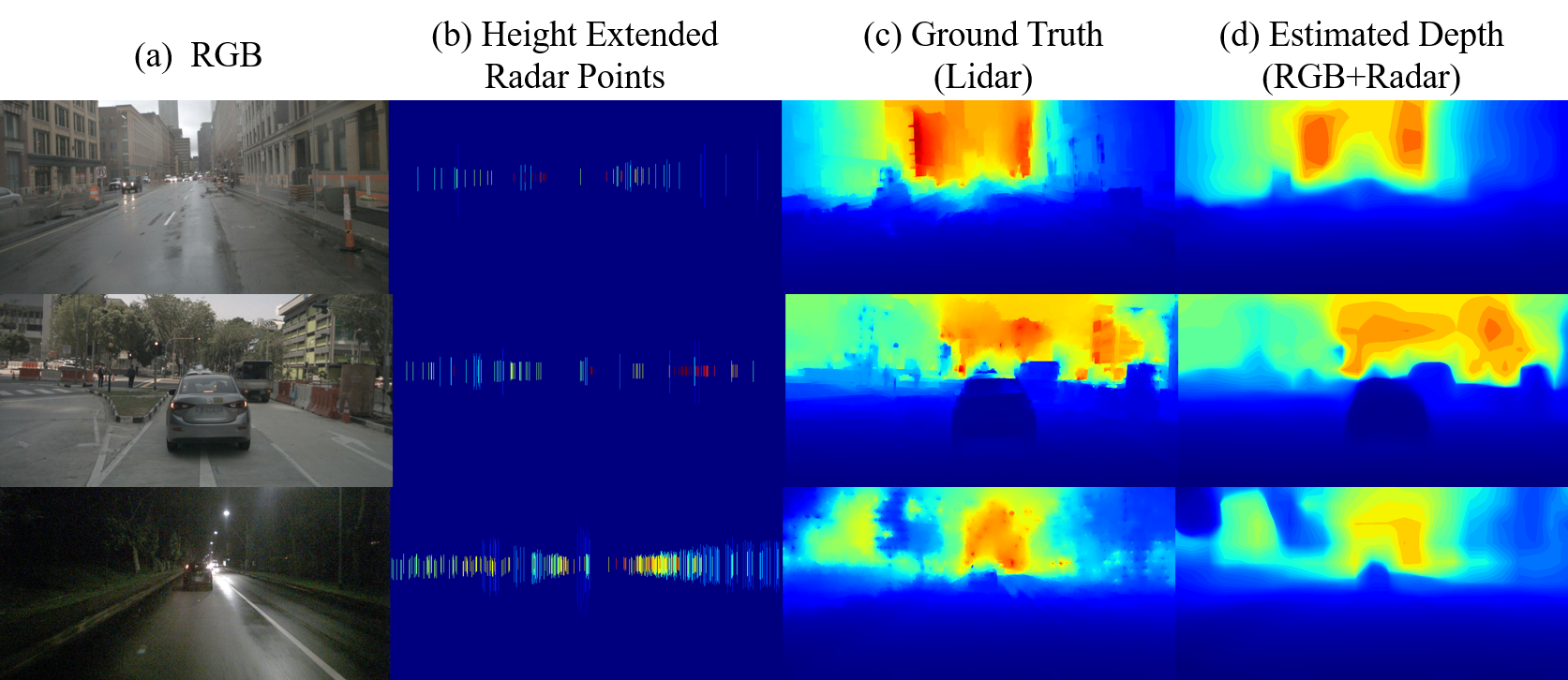
Figure 3: The qualitative results of depth estimation using RGB+Radar with only extended radar’s point cloud.

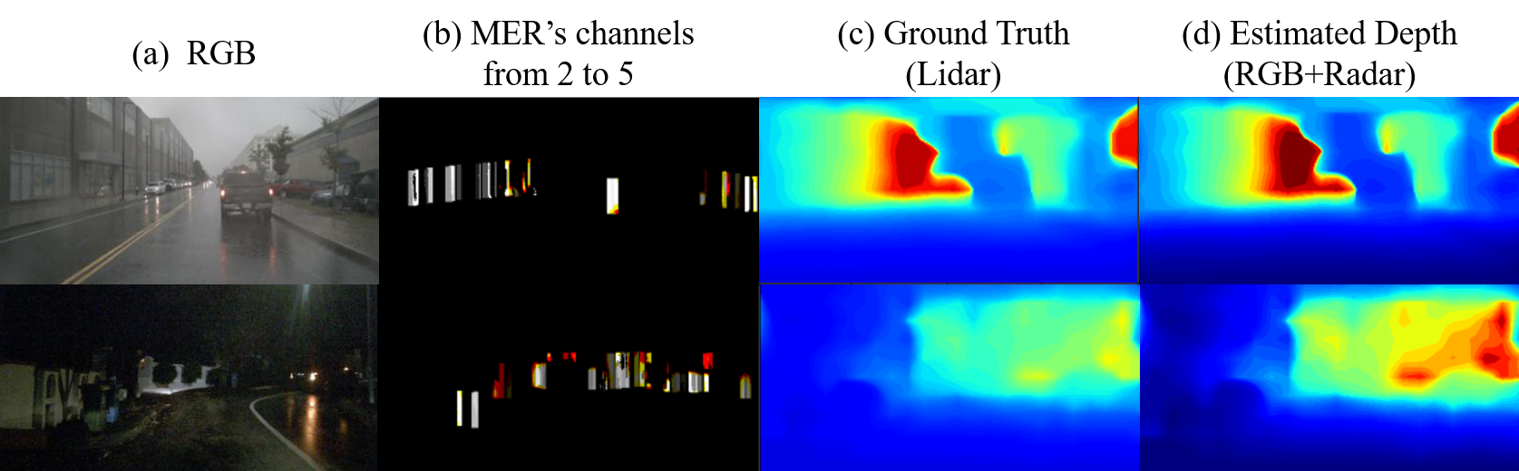
Figure 4: The qualitative results are based on RGB+MERs radar point cloud.

III-A Feature Pyramid Network (FPN)

Feature pyramid network is a unique composition of CNN where the connection graph is bifurcated after selected layers, and the features are scaled down on one path and used with scaled-up features returning from the bottleneck on the other path as shown in Fig 2. A residual network is often used as a backbone of FPN. The residual network comprises convolution blocks enclosed into a residual block, and networks of different depths combine multiple residual blocks in varied numbers. The output of each residual block usually forms a layer of FPN and learns features at multiple scales. However, using all features at all available pyramid levels is expensive and adds extensive computation cost. In this work, we use three pyramid feature layers. Furthermore, our network adds a variation in the use of pyramid features. It up-samples the pyramid features at different scales, concatenates them, and uses them with radar features. Monocular depth estimation is an ill-posed problem and estimating depth with multi-scale features puts this work on the edge and it predicts better estimation maps than competitive CNN approaches. It exploits rich semantics from top-down lateral connections to bottom-up using convolutional layers, while concatenating the robust features in lower resolutions semantics and weak features in high-resolution semantics.

III-B Modified FPN Composition

[14] computes the pyramid levels using top-down and the lateral connection. FPN pyramid layers from P3 to P5 (Fig. 2) are connected to corresponding layers in the residual network (C2 to C4) in reverse order. P6 is computed with a convolution filter of size (3x3) with a stride of (2) from C4. However, P7 is obtained from similar convolution composition with P6. In this research, we only use pyramid features (P3 to P5) and exclude P6 and P7. A rationale is that the up-sampling on feature pyramids (P3 to P5) cater for the fine-grained features of P6 and P7. This reduction of the fine-grained pyramid layers decreases the parameters significantly, thus reducing the computation cost.

III-C Radar and RGB Data Fusion

A late fusion technique has opted in this study, and radar data is encoded using a separate ResNet. Since the radar point cloud data is sparse, it is a practice to extend the radar data. The details of the augmentation process are given in section III-E. A rationale for using a separate radar data network is masking coarse radar data by fine-grained RGB data in CNN when learned together. This study uses ResNet-18 for extracting features from the radar data. The features from both the sensors are fused, and the accurate distance information validates the purposive depth relationship among RGB features.

III-D Ordinal Regression Layer

In monocular depth estimation, a depth value is estimated in a given range of real-valued distances for each pixel in an image. Moreover, the learning process is guided by the accumulated loss computed using the difference between predicted and estimated depths for all pixels. However, 2D image inherits depth semantics of perspective projection aspect ratio, which reveals two issues: First, during training, the difference between depth error is highly varied, and second, the distance in active closer regions is pronounced when compared to the distant regions, which is inversely proportional to the error in depth estimation. Ordinal regression resolves the two issues by mapping the regression problem to a classification problem. Ordinal regression divides the real-valued distances into bins, and bins are monotonically increasing functions of the distance. The bins normalize the backpropagated gradient value of the calculated loss for all the pixels. Furthermore, monotonically increasing binning caters to the semantics of perspective projection ratios. The ordinal regression is often computed in log space discrete values which represent bins and further enforce the perspective projection ratios and normalized error computation. In this work, we opted ordinal regression layer composition and loss function as discussed in [7], [5]. The modified feature pyramid network adds a hard inductive bias to the monocular image features suited for the depth estimation and prior conditioning with radar data serves better prediction in scenes where the image data is not sufficient. Moreover, the radar data provides an implicit anchoring for pixels to depth classification with an ordinal regression module. The unified approach makes a valuable addition to the SOTA with simple modules.

III-E Radar data augmentation using radar channel Enhancement (MER’s)

The final investigation in this study considers the extension of sparse point cloud radar data to meaningful presentation. In the first approach, we use markers’ extension in height only as shown in the second column of Fig. 3. However, it also enhances the noise captured by the radar. A second approach extends markers with the help of their corresponding neighboring pixels in the image and estimates pixels to depth association (PDA)[16] using a DNN supervised with lidar point cloud data. It expands the width and height of the markers, and it defines a separate channel for different confidence levels of an association called multiple channel-based enhanced radar image (MER) (Fig. 3 column-3). MER estimates the extended heights and width of the region that may be occupied by an object in the actual scene. The simple height extension of radar data elongates the height in the form of strips. Whereas MERs use a trained ANN for predicting the height and width extension in the neighboring regions of the radar markers. MERs also predict the neighboring region based on a threshold and confidence. Also with the lower confidence values of the neighboring regions, it defines multiple channels of different confidence ranges.

Results on Full nuScenes Dataset
Method	$\delta_{1}\uparrow$					$RMSE\downarrow$					$AbsRel\downarrow$
	combine	day	night	rain		combine	day	night	rain		combine	day	night	rain
RGB	$0.88$	$0.88$	$0.77$	$0.88$		$5.30$	$5.10$	$6.79$	$5.39$		$0.11$	$0.11$	$0.16$	$0.10$
Lin et al.[2]	$0.88$	$0.89$	$\mathbf{0.81}$	$-$		$5.40$	$5.27$	$6.40$	$-$		$0.11$	$0.10$	$\mathbf{0.14}$	$-$
Cho et al. [5]	$0.88$	$0.90$	$0.78$	$0.88$		$5.19$	$4.97$	$6.86$	$5.48$		$0.10$	$0.10$	$0.15$	$0.10$
Stefano, et al. [6]	$-$	$0.86$	$-$	$-$		$-$	$6.43$	$-$	$-$		$0.13$	$0.12$	$0.21$	$0.14$
Ours (RVMDE)	$\mathbf{0.90}$	$\mathbf{0.91}$	$\mathbf{0.81}$	$\mathbf{0.91}$		$\mathbf{5.06}$	$\mathbf{4.83}$	$6.57$	$\mathbf{4.98}$		$\mathbf{0.10}$	$\mathbf{0.10}$	$\mathbf{0.14}$	$\mathbf{0.09}$
Ours RVMDE with MERs	$\mathbf{0.90}$	$\mathbf{0.91}$	$0.79$	$\mathbf{0.91}$		$\mathbf{3.54}$	$\mathbf{3.39}$	$\mathbf{5.16}$	$\mathbf{3.40}$		$\mathbf{0.10}$	$\mathbf{0.09}$	$0.15$	$0.10$

TABLE I: We evaluated the Proposed and the other SOTA models’ results. Capture all the scenarios category-wise (clear day scenario, rain scenario, and night scenarios) on the test set—a late fusion is applied using both the sensor modalities (monocular images and radar).

Evaluation on Full nuScenes Dataset with MER’s - Estimation error with low height region (0.3 to 2(meters) above the ground level)
method	$\delta_{1}\uparrow$					$RMSE\downarrow$					$AbsRel\downarrow$					$RMSE_{log}\downarrow$
	combine	day	night	rain		combine	day	night	rain		combine	day	night	rain		combine	day	night	rain
Cho et al. [5]	$0.74$	$0.75$	$0.65$	$0.77$		$5.10$	$5.13$	$6.42$	$4.80$		$0.18$	$0.18$	$0.19$	$0.19$		$0.24$	$0.24$	$0.30$	$0.24$
HourglassNet [30]	$0.81$	$0.82$	$0.72$	$0.80$		$4.22$	$4.18$	$4.87$	$4.11$		$0.14$	$0.14$	$0.17$	$0.16$		$0.20$	$0.20$	$0.23$	$0.21$
Ours (RVMDE)	$\mathbf{0.84}$	$\mathbf{0.84}$	$\mathbf{0.75}$	$\mathbf{0.86}$		$\mathbf{4.15}$	$\mathbf{4.14}$	$\mathbf{4.75}$	$\mathbf{3.95}$		$\mathbf{0.14}$	$\mathbf{0.13}$	$\mathbf{0.17}$	$\mathbf{0.13}$		$\mathbf{0.19}$	$\mathbf{0.19}$	$\mathbf{0.23}$	$\mathbf{0.13}$
MER’s (Multi-Enhanced Radar Channels) - Evaluation on Full-image depth completion errors (m)
Cho et al. [5]	$0.84$	$0.85$	$0.68$	$0.86$		$4.44$	$4.27$	$5.67$	$4.23$		$0.13$	$0.13$	$0.18$	$0.13$		$0.19$	$0.19$	$0.27$	$0.24$
HourglassNet [30]	$0.86$	$0.87$	$0.75$	$0.87$		$3.98$	$3.84$	$5.55$	$3.86$		$0.11$	$0.10$	$0.16$	$0.11$		$0.18$	$0.17$	$0.24$	$0.18$
Ours (RVMDE)	$\mathbf{0.90}$	$\mathbf{0.91}$	$\mathbf{0.79}$	$\mathbf{0.91}$		$\mathbf{3.54}$	$\mathbf{3.39}$	$\mathbf{5.16}$	$\mathbf{3.40}$		$\mathbf{0.10}$	$\mathbf{0.09}$	$\mathbf{0.15}$	$\mathbf{0.10}$		$\mathbf{0.15}$	$\mathbf{0.15}$	$\mathbf{0.23}$	$\mathbf{0.15}$

TABLE II: Proposed models (RVMDE), results based on Multiple channel based enhanced radar (MER), image.

IV Experimental Work

IV-A Dataset

We performed all experiments on nuScenes dataset [1], which covers various environmental conditions data. The dataset is collected on Singapore and Boston roads for almost 15 hours of driving in varying conditions, including rain, night, daylight, lighting, and varying illuminations. The vehicle is mounted with 1 x lidar, 6 x cameras, and 5 x radars, covering a 360-degree field of view (FOV) in each scene. The complete dataset contains 1000 scenes, of which 850 scenes are annotated. The dataset draws an average of 40 samples in 20 seconds of driving from each scene. Moreover, the nuScenes dataset comes with a development kit that calibrates the sensors and projects data from one sensor to another. Similar to [2], we utilized 850 labeled scenes and split them into 750 training, 15 validation, and 85 test sets for a fair comparison with the SOTA. There are 30736 sample frames in 850 scenes selected for training and 3424 sample frames for evaluation. In this study, the front camera images and the overlapped radar point cloud data are used. In the official dataset, there are no depth annotations available, so we follow [2], and use the lidar’s point cloud information as ground truth [37].

IV-B Implementation Details

The experiments are performed on 24GB Nvidia-GTX-3090, with 48GB internal memory on a single machine, and implemented in PyTorch [8] framework. For training the model, we use a batch size of 8 with stochastic gradient descent (SGD) as an optimizer. Initially, the learning rate is set to 0.001 with polynomial power of 0.9. The momentum is set to 0.9 with a weight decay of 0.0001 after every ten epochs. The backbone network is initialized with ImageNet pre-trained [38], for RGB, and random weights are assigned to the sparse radar. The network is trained for 40 epochs. We use ordinal regression as space increasing discretization (SID) similar to [7] and train the network with ordinal regression loss [7]. In this study we follow [7] and use 80 intervals for the ordinal regression. The fewer number of intervals add quantization error, while the larger number of intervals create non-discretization. For a fair comparison, we set the same parameters for all SOTA techniques and compute results. The training and evaluation are performed with down-scaled images from 900 x 1600 to 450 x 900 resolution that is further reduced by truncating the top 100 pixels in height. The exact resolution is used for projecting the radar points and for generating the ground truth using lidar.

Results on Complete nuScenes (Higher $\delta$ value is better)
Methods	$\delta_{1}<1.25$	$\delta_{2}<1.25^{2}$	$\delta_{3}<1.25^{3}$
PnP [10]	$0.86$	$0.94$	$0.97$
Cho et al. [5]	$0.88$	$-$	$-$
Sparse-to-dense [3]	$0.87$	$0.94$	$0.97$
CSPN [27]	$0.86$	$0.94$	$0.97$
Lin et al. [2]	$0.88$	$0.95$	$0.97$
Ours (RVMDE)	$\mathbf{0.90}$	$\mathbf{0.96}$	$\mathbf{0.98}$

TABLE III: Comparison between Proposed and SOTA models.

Methods	$\delta_{1}<1.25$	$\delta_{2}<1.25^{2}$	$\delta_{3}<1.25^{3}$
Cho et al. [5] with MER	$0.74$	$0.91$	$0.96$
Hourglass [30] with MER	$0.81$	$0.94$	$0.97$
(RVMDE) with MER	$\mathbf{0.84}$	$\mathbf{0.95}$	$\mathbf{0.98}$

TABLE IV: Results on Full nuScenes Dataset with MER’s - Evaluation on Low-height region (0.3 to 2(meters) above the ground level).

Methods	$\delta_{1}<1.25$	$\delta_{2}<1.25^{2}$	$\delta_{3}<1.25^{3}$
Cho et al. [5] with MER	$0.84$	$0.94$	$0.97$
Hourglass [30] with MER	$0.86$	$0.95$	$0.98$
(RVMDE) with MER	$\mathbf{0.90}$	$\mathbf{0.97}$	$\mathbf{0.99}$

TABLE V: On Full nuScenes Dataset with MER’s - Evaluation on Full-image depth completion errors (m)

IV-C Experimentation and Results

In this research, we use nuscenes dataset for experimentation and compares with state-of-the-art with monocular depth estimation with radar data on the dataset. Moreover, a detailed experimentation on all given scene categories in the dataset (day, night, and rain scenarios) [1] is performed to verify the efficacy of the proposed strategy. The experiments are divided into two major categories: The first category uses the height extended radar markers, while the second experiment uses multiple channel enhanced radar (MER’s) as discussed in the above section III. The proposed RVMDE architecture is used in both experiments with same hyperparameters. The only difference is the number of input channels for the first convolutional layer of backbone CNN to incorporate the MERs data input. The trainable parameters in proposed architecture are 68 million, which is approximately half to a similar architecture used in [5]. In this study, MERs computes six confidence intervals and the values are adopted from [16]. The inference time for a batch of size three on the used GPU takes 0.118 sec, almost half of the time for existing models ([5]) which takes 0.221 sec.

A comparison with the state-of-the-art monocular depth estimation with radar data fusion on all the environmental conditions is detailed in Table I. The evaluation metrics for qualitative results are Root Mean Square Error ($RMSE$), ($RMSE_{log}$), Absolute Relative Error ($AbsReL$) and threshold $\delta_{1},\delta_{2},\delta_{3}$ [2], [3]. Table I shows the quantitative results produced using height extended radar marker as input, and Table II shows the results of the depth estimation with MERs inputs. The results of compared techniques are generated using the provided code by the cited works. To the best of our knowledge, only Chen et al. [5] provides their experimental results on the complete nuScenes dataset. Juan. et al. [2] highlighted the day and night scene results only. Overall, the proposed model outperformed and improved almost every situation and reduces the inference time.

The threshold limit-wise $\delta$ results are placed in Table-III, IV, V. In all the categories of evaluation metrics, the proposed models’ results are improved quantitatively. The qualitative results are placed in Fig. 3 and Fig. 4. The proposed method’s superiority over the Hourglass network [30] could be the simplicity of the model and its inductive bias support for the problem at hand. More can be found out with experiments in different domains and their comparison, but for now, we reiterate the phenomenon of the no-free lunch theorem.

V Ablation Study

We conducted two ablation studies: First, generalization is tested by training and tested in different scenes for all available imaging conditions in the nuScence dataset, and second, the effectiveness of ordinal regression is evaluated against simple regression. Table VI shows the qualitative results obtained by reducing the training data of the rain, day, and night dataset. We train the proposed model (RVMDE+Mers) with the same parameters and tested the trained model on scenes different from the training data. The qualitative results show insignificant variation from the results presented in Table II. In the second experiment, we change the loss function to check the ordinal regression loss ability in terms of accurate depth estimation for a range of 80 meters. The experiments use L1 (Mean Absolute Error) [32] and L2 (Mean Square Error) [33] regression losses instead of ordinal regression loss. Model is trained with the same parameters except changing the loss function but the model was unable to produce equivalent results. Table VII shows the qualitative results with two alternate regression loss functions and asserts the use of ordinal regression loss in the proposed technique for the depth estimation task.

Different training and testing scenes experiment for ablation study
Methods	$\delta_{1}\uparrow$	$RMSE\downarrow$	$AbsRel\downarrow$	$RMSE_{log}\downarrow$
Day	$0.88$	$3.76$	$0.11$	$0.17$
Night	$0.70$	$5.73$	$0.19$	$0.25$
Rain	$0.87$	$3.96$	$0.12$	$0.18$

TABLE VI: Reducing training nuScenes Dataset (Day, Night, Rain) separately with MER’s - Evaluation on Full-image depth completion errors (m)

Proposed Model (RVMDE) on Full nuScenes with different Loss
Loss Function	$\delta_{1}\uparrow$	$RMSE\downarrow$	$AbsRel\downarrow$	$RMSE_{log}\downarrow$
MAE $L1$	$0.79$	$7.39$	$0.14$	$0.24$
MSE $L2$	$0.76$	$7.59$	$0.13$	$0.25$
Ordinal Reg Loss	$0.90$	$5.06$	$0.10$	$0.15$

TABLE VII: Applying Different Loss Function

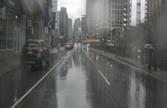
(a) Camera image

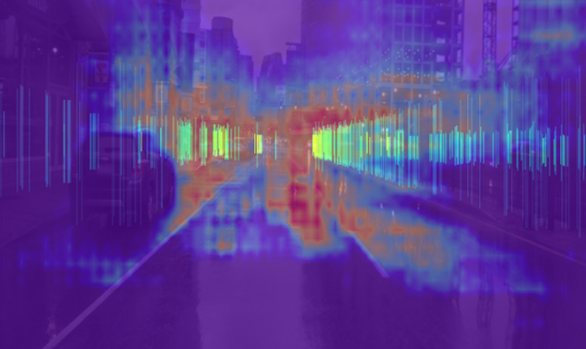
(b) RaDorn Distance at 33m

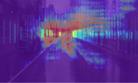
(c) RaDorn Distance at 55m

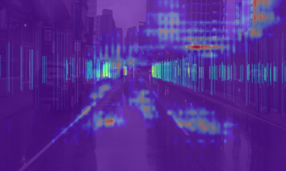
(d) RaDorn Distance at 70m

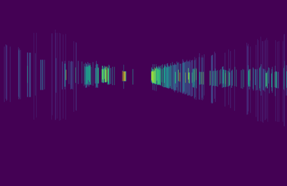
(e) Height extended Radar Markers

(f) RVMDE Distance at 35m

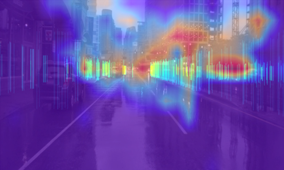
(g) RVMDE Distance at 55m

(h) RVMDE Distance at 70m

Figure 5: The radar markers are projected to visualise the effect of radar information at different distance by using CAM approach. (a) is RGB test image and (b), (c), (d) are RaDorn results with distance values of 35m, 55m, and 70m respectively. (e) shows calibrated height extended radar points for corresponding test image. (f), (g) and (h) depicts activation maps generated with results computed with the proposed RVMDE at same distance values.

V-A Class Activation Maps

Furthermore, we evaluate the effects of adding radar markers and pyramid feature layers using activation maps. The ordinal regression enables the usage of GRAD-CAM++ [42] using the distance classes. Grad-CAM++ uses the derivatives of the convolution feature maps weighted with scores of a particular distance class to identify the portion in the test image participating in the decision. Fig. 5 depicts the results of the CAM generated for the monocular depth estimation with and without radar data. The selected frames are tested with distance values of 35m, 55m, and 70m. It is evident from the RVDME generated depth estimation results that the regions validated with the radar markers actively participate in depth estimation. Whereas the images only depth estimation is dominated by the vanishing point phenomenon in perspective projection. Moreover, the pyramid feature network keeps the spacial locality intact in addition to the scale invariance properties. Therefore, CAM tests provide an insight into the usage of individual sensors’ input in data fusion and particularly the effectiveness of radar markers for the validation of ill-posed monocular depth estimation problems.

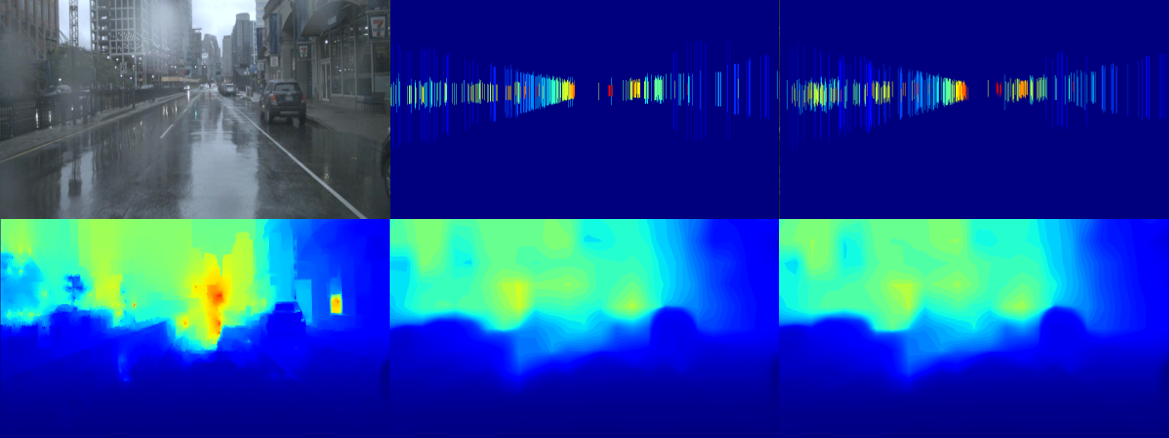
Figure 6: From left to right (a) RGB (b) Height extended radar points with calibration error (c) Calibrated height extended radar points. In second row left to right (a) Ground truth (lidar) (b) Depth Estimation with calibration error of height extended radar points (c) With calibrated height extended radar points final depth estimation. The qualitative results of depth estimation by actual and interrupted calibration changing the radar camera calibration using RGB+Radar with only extended radar’s point cloud.

V-B Extended Discussion

The proposed method assumes that the sensors are calibrated and can fail to produce accurate reported results if the calibration parameters have calibration errors. We experimented to evaluate the proposed method by modifying the calibration parameters which disturb the transformation as shown in Fig. 6. The first row part (c) shows the radar markers with synthetically induced noise, whereas the second row part (c) is the actual radar markers. It is observed that the depth estimation part (d) tolerates noise induced by the error in sensors calibration. However, the bounds are not studied in detail for this work and may be carried out in future works. Moreover, the ground truth is dependent on the lidar sensor. As the nuScenes dataset does not provide the ground truth for monocular camera depth, we utilize the lidar sensor information for ground truth. Thus the synchronization between the sensors (lidar camera and radar) is mandatory for better predictions.

VI Conclusion

This study demonstrates the utility of a variant of the feature pyramid network (FPN) for radar validated monocular depth estimation for robotics applications. The proposed FPN uses up-sampled lower feature pyramid layers instead of the two higher feature pyramid layers to reduce the number of parameters. The up-sampling caters to the features captured in higher layers. The augmented radar data is fused with the RGB image data in late fusion composition, which guides the ill-posed estimation problem with factual depth information. An ordinal regression layer is added to map the conventional depth estimation regression problem to a classification problem. The results show that the proposed technique outperformed SOTA tested on a complete nuScenes dataset in various environmental conditions. Anticipated future directions are to use a simple radar and image data association technique. Another challenge that needs further investigation is to detect spoofing in monocular depth estimation with radar data fusion.

References

- [1] H. Caesar, V. Bankiti, A. H. Lang, S. Vora, V. E. Liong, Q. Xu, A. Krishnan, Y. Pan, G. Baldan, and O. Beijbom, “nuscenes: A multimodal dataset for autonomous driving,” in IEEE Conference on Computer Vision and Pattern Recognition (CVPR),
- [2] Juan-Ting Lin, Dengxin Dai, and Luc Van Gool, “Depth Estimation from Monocular Images and Sparse Radar Data,” in IEEE International Conference on Intelligent Robots and Systems (IROS),
- [3] F. Mal and S. Karaman, ”Sparse-to-dense: Depth prediction from sparse depth samples and a single image,” in IEEE International Conference on Robotics and Automation (ICRA),
- [4] F. Ma, G. V. Cavalheiro, and S. Karaman, ”Self-supervised sparse-to-dense: Self-supervised depth completion from lidar and monocular camera,” in IEEE International Conference on Robotics and Automation (ICRA),
- [5] Lo, Chen-Chou, and Patrick Vandewalle. ”Depth Estimation From Monocular Images And Sparse Radar Using Deep Ordinal Regression Network.” 2021 IEEE International Conference on Image Processing (ICIP). IEEE,
- [6] Gasperini, Stefano, et al. ”R4Dyn: Exploring Radar for Self-Supervised Monocular Depth Estimation of Dynamic Scenes.” arXiv preprint arXiv:2108.04814
- [7] H. Fu, M. Gong, C. Wang, K. Batmanghelich, and D. Tao, ”Deep ordinal regression network for monocular depth estimation,” in IEEE Conference on Computer Vision and Pattern Recognition (CVPR),
- [8] Adam Paszke, Sam Gross, Francisco Massa, Adam Lerer, James Bradbury, Gregory Chanan, Trevor Killeen, Zeming Lin, Natalia Gimelshein, Luca Antiga, et al. Pytorch: An imperative style, high-performance deep learning library. In Advances in Neural Information Processing Systems,
- [9] F. Nobis, M. Geisslinger, M. Weber, J. Betz, and M. Lienkamp, ”A deep learning-based radar and camera sensor fusion architecture for object detection,” in Sensor Data Fusion: Trends, Solutions, Applications (SDF),
- [10] T.-H. Wang, F.-E. Wang, J.-T. Lin, Y.-H. Tsai, W.-C. Chiu, and M. Sun, ”Plug-and-play: Improve depth estimation via sparse data propagation,” in International Conference on Robotics and Automation (ICRA),
- [11] Kaiming He, X. Zhang, Shaoqing Ren, and Jian Sun, “Deep residual learning for image recognition,” 2016 IEEE Conference on Computer Vision and Pattern Recognition (CVPR), pp. 770–778, 2016.
- [12] A. Roy and S. Todorovic, “Monocular depth estimation using neural regression forest,” in 2016 IEEE Conference on Computer Vision and Pattern Recognition (CVPR),
- [13] Lin, Tsung-Yi, et al. ”Focal loss for dense object detection.” Proceedings of the IEEE international conference on computer vision.
- [14] T.-Y. Lin, P. Dollar, R. Girshick, K. He, B. Hariharan, and S. Belongie. Feature pyramid networks for object detection. In Proceedings of the IEEE Conference on Computer Vision and Pattern Recognition, (CVPR)
- [15] S. Chadwick, W. Maddern, and P. Newman, ”Distant vehicle detection using radar and vision,” International Conference on Robotics and Automation (ICRA),
- [16] Yunfei Long, Daniel Morris, Xiaoming Liu, Marcos Castro, Punarjay Chakravarty, and Praveen Narayanan. Radarcamera pixel depth association for depth completion. In IEEE Conference on Computer Vision and Pattern Recognition (CVPR),
- [17] Youngseok Kim, Jun Won Choi, and Dongsuk Kum. GRIF Net: Gated region of interest fusion network for robust 3d object detection from radar point cloud and monocular image. In 2020 IEEE/RSJ International Conference on Intelligent Robots and Systems (IROS),
- [18] J. Flynn, I. Neulander, J. Philbin, and N. Snavely, “Deepstereo: Learning to predict new views from the world’s imagery,” in IEEE Conference on Computer Vision and Pattern Recognition (CVPR),
- [19] A. Saxena, M. Sun, and A. Y. Ng, “Make3d: Learning 3d scene structure from a single still image,” IEEE Transactions on Pattern Analysis and Machine Intelligence (TPAMI),
- [20] L. Ladicky, J. Shi, and M. Pollefeys, “Pulling things out of perspective,” in IEEE Conference on Computer Vision and Pattern Recognition (CVPR),
- [21] A. Geiger, P. Lenz, and R. Urtasun, “Are we ready for autonomous driving? the kitti vision benchmark suite,” in IEEE Conference on Computer Vision and Pattern Recognition (CVPR),
- [22] M. Cordts, M. Omran, S. Ramos, T. Rehfeld, M. Enzweiler, R. Benenson, U. Franke, S. Roth, and B. Schiele, “The cityscapes dataset for semantic urban scene understanding,” in IEEE Conference on Computer Vision and Pattern Recognition (CVPR),
- [23] K. Simonyan and A. Zisserman, “Very deep convolutional networks for large-scale image recognition,” in International Conference on Learning Representations (ICLR),
- [24] K. He, G. Gkioxari, P. Dollár, and R. Girshick, “Mask r-cnn,” in IEEE International Conference on Computer Vision (ICCV), .
- [25] D. Eigen and R. Fergus, “Predicting depth, surface normals and semantic labels with a common multi-scale convolutional architecture,” in IEEE International Conference on Computer Vision (ICCV),
- [26] J. Xie, R. Girshick, and A. Farhadi, “Deep3d: Fully automatic 2d-to-3d video conversion with deep convolutional neural networks,” in European Conference on Computer Vision (ECCV),
- [27] X. Cheng, P. Wang, and R. Yang, “Depth estimation via affinity learned with convolutional spatial propagation network,” in European Conference on Computer Vision (ECCV),
- [28] Hamid Laga, “A survey on deep learning architectures for image-based depth reconstruction,” arXiv preprint arXiv:1906.06113,
- [29] Tian, Yuan, and Xiaodong Hu. ”Monocular depth estimation based on a single image: a literature review.” Twelfth International Conference on Graphics and Image Processing (ICGIP 2020). Vol. 11720. International Society for Optics and Photonics,
- [30] Ang Li, Zejian Yuan, Yonggen Ling, Wanchao Chi, Chong Zhang, et al. ”A multi-scale guided cascade hourglass network for depth completion”. In IEEE Winter Conference on Applications of Computer Vision, pages 32–40,
- [31] http:
- [32] Mean absolute error. In Claude Sammut and Geoffrey I.Webb, editors, ”Encyclopedia of Machine Learning”, page 652. Springer, .
- [33] Mean squared error. In Claude Sammut and Geoffrey I.Webb, editors, ”Encyclopedia of Machine Learning and Data Mining”, page 808. Springer, .
- [34] R. Garg, V. K. BG, G. Carneiro, and I. Reid, “Unsupervised cnn for single view depth estimation: Geometry to the rescue,” in European Conference on Computer Vision (ECCV), .
- [35] J. Li, R. Klein, and A. Yao, “A two-streamed network for estimating fine-scaled depth maps from single rgb images,” in IEEE International Conference on Computer Vision (ICCV), .
- [36] J. Xie, R. Girshick, and A. Farhadi, “Deep3d: Fully automatic 2dto-3d video conversion with deep convolutional neural networks,” in European Conference on Computer Vision (ECCV), .
- [37] F. Ma, G. V. Cavalheiro, and S. Karaman, “Self-supervised sparseto-dense: Self-supervised depth completion from lidar and monocular camera,” in IEEE International Conference on Robotics and Automation (ICRA),
- [38] J. Deng, W. Dong, R. Socher, L.-J. Li, K. Li, and L. Fei-Fei, “Imagenet: A large-scale hierarchical image database,” in IEEE Conference on Computer Vision and Pattern Recognition (CVPR),
- [39] Zhao, Chaoqiang, et al. ”Monocular depth estimation based on deep learning: An overview.” Science China Technological Sciences
- [40] Ming, Yue, et al. ”Deep learning for monocular depth estimation: A review.” Neurocomputing
- [41] Khan, Faisal, Saqib Salahuddin, and Hossein Javidnia. ”Deep learning-based monocular depth estimation methods—A state-of-the-art review.” Sensors
- [42] A. Chattopadhay, A. Sarkar, P. Howlader and V. N. Balasubramanian. ”Grad-CAM++: Generalized Gradient-Based Visual Explanations for Deep Convolutional Networks,” 2018 IEEE Winter Conference on Applications of Computer Vision (WACV), 2018, pp. 839-847, doi: 10.1109/WACV.2018.00097.