A novel high dimensional fitted scheme for stochastic optimal control problems

Abstract

Stochastic optimal principle leads to the resolution of a partial differential equation (PDE), namely the Hamilton-Jacobi-Bellman (HJB) equation. In general, this equation cannot be solved analytically, thus numerical algorithms are the only tools to provide accurate approximations. The aims of this paper is to introduce a novel fitted finite volume method to solve high dimensional degenerated HJB equation from stochastic optimal control problems in high dimension ($n\geq 3$). The challenge here is due to the nature of our HJB equation which is a degenerated second-order partial differential equation coupled with an optimization problem. For such problems, standard scheme such as finite difference method losses its monotonicity and therefore the convergence toward the viscosity solution may not be guarantee. We discretize the HJB equation using the fitted finite volume method, well known to tackle degenerated PDEs, while the time discretisation is performed using the Implicit Euler scheme.. We show that matrices resulting from spatial discretization and temporal discretization are M–matrices. Numerical results in finance demonstrating the accuracy of the proposed numerical method comparing to the standard finite difference method are provided.

1 Introduction

The theory of optimal control for stochastic differential equations is mathematically challenging and it has been considered in many fields such as economics, engineering, biology and finance WH2 , HP . Stochastic optimal control problems have been studied by many researches KL , JER , HPFH . In some cases, the well posedness of such problems have been studied using methods such as viscosity and minimax techniques (see Cra1 , Cra2 , Cra5 ). In general, most of them do not have an explicit solution, therefore there have been many attempts to develop novel methods for their approximations. Numerical approximation of stochastic optimal control problem is therefore an active research area and has attracted a lot of attentions Cra7 , KNV1 , KL1 , KL , JER , HPFH . The keys challenge for solving HJB equation are the low regularity of the solution and the lack of appropriate numerical methods to tackle the degeneracy of the differential operator in HJB equation. Indeed adding to the standard issue that we usually have when solving degenerated PDE, we need to couple with an optimization problem at each point of the grid and for each time step. A standard approach is based on Markov chain approximation, which suffers from time step limitations due to stability issues Peter as the method is indeed based on finite difference approach. Many stochastic optimal control problems such as Merton optimal problems have degenerated linear operator when the spatial variables approach the region near to zero. This degeneracy has an adverse impact on the accuracy when the finite difference method is used to solve such optimal problems 15 , wilmott2005best as the monotonicity of the scheme is usually lost. However, when solving HJB equation, the monotonicity also plays a key role to ensure the convergence of the numerical scheme toward the viscosity solution. Indeed in high dimensional Merton’s control problem, the matrix in the diffusion part is lower rank near the origin and it has been found in chistoph2019 , chistoph2020 that the standard finite difference schemes become non monotone and may not converge to the viscosity solution of the HJB. To solve the degeneracy issue, a fitted finite volume have been proposed in 15 for one and two dimensional optimal control problems. This method uses special technique called fitted technique to tackle the degeneracy. The scheme have been initially developed to solve Black Scholes PDEs for options pricing (see WS and references therein). In 15 , numerical experiments have been used to demonstrate that the fitted finite volume scheme is more accurate than the standard finite difference approach to approximate one and two dimensional stochastic optimal problems. To the best of our knowledge, even for Black Scholes PDEs for options pricing, fitted technique for high dimensional domain ($n\geq 3$) has be lacked in the literature.

The aim of this research is to introduce the first fitted finite volume method for stochastic optimal control problems in high dimensional domain ($n\geq 3$). This method is suitable to handle the degeneracy of the linear operator while solving numerically the HJB equation. The method is coupled with implicit time-stepping method and the iterative method presented in HPFH for optimization problem at every time step. The merit of the method is that it is absolutely stable in time because of the implicit nature of the time discretisation and yields a linear system with a positive-definite $M$-matrix, this is in contrast of the standard finite difference scheme.

The novel contribution of our paper over the existing literature can be summarized as

• We have upgraded the fitted finite volume technique to discretize a more generalized HJB equation coupled with the implicit time-stepping method for temporal discretization method and the iterative method for the optimization problem at every time step. To best of our knowledge such combination has not yet proposed so far to solve stochastic optimal control problems in high dimensional domain ($n\geq 3$).

• We have proved that the corresponding matrices after spatial and temporal discretization are positive-definite $M$–matrices. We have demonstrated by numerical experiments that the proposed scheme can be more accurate than the standard finite difference scheme.

The rest of the paper is organized as follows. The stochastic optimal control problems is introduced in section2. In section 3, we introduce the fitted finite volume in high dimensional domain and show that the system matrix of the resulting discrete equations is an $M$-matrix. Section 5 provides temporal discretization and optimization algorithm for spatial diiscretized HJB equation. In section 6, we present some numerical examples illustrating the accuracy of the proposed method comparing to the standard finite difference. Finally, in section 7, we summarise our finding.

2 Preliminaries and formulation

Let $\left(\Omega,\mathcal{F},\mathbb{F}=(\mathcal{F}_{t})_{t\geq 0},\mathbb{P}\right)$ be a filtrated probability space. We consider the numerical approximation of the following controlled Stochastic Differential Equation (SDE) defined in $\mathbb{R}^{n}$ by

$$\begin{split}&dx_{s}=b(s,x_{s},\alpha_{s})dt+\sigma(s,x_{s},\alpha_{s})d\omega_{s},\,\,\,s\,\in(t,T]\\ &x_{t}=x\end{split}$$ (1)

where

$$\begin{split}b&:[0,T]\times\mathbb{R}^{n}\times\mathcal{A}\rightarrow\mathbb{R}^{n}\\ &(t,x_{t},\alpha_{t})\rightarrow b(t,x_{t},\alpha_{t})\end{split}$$ (2)

is the drift term and

$$\begin{split}\sigma&:[0,T]\times\mathbb{R}^{n}\times\mathcal{A}\rightarrow\mathbb{R}^{n\times d}\\ &(t,x_{t},\alpha_{t})\rightarrow\sigma(t,x_{t},\alpha_{t})\end{split}$$ (3)

the $d$-dimensional diffusion coefficients. Note that $\omega_{t}$ are $d$-dimensional independent Brownian motion on $\left(\Omega,\mathcal{F},(\mathcal{F}_{t})_{t\geq 0},\mathbb{P}\right)$, the control $\alpha=(\alpha_{t})_{t\geq 0}$ is an $\mathbb{F}$-adapted process, valued in $\mathcal{A}$ compact convex subset of $\mathbb{R}^{m}\,(m\geq 1)$ and satisfying some integrability conditions and/or state constraints. Precise assumptions on $b$ and $\sigma$ to ensure the existence of the unique solution $x_{t}$ of (1) can be found in HP .
Given a function $f$ from $[0,T]\times\mathbb{R}^{n}\times\mathcal{A}$ into $\mathbb{R}$ and $g$ from $\mathbb{R}^{n}$ into $\mathbb{R}$, the performance functional is defined as

$$J(t,x,\alpha)=\mathbb{E}\,\left[\int_{t}^{T}f(s,x_{s},\alpha)\,ds+g(x_{T})\right],\,\,\,\forall\,x\,\in\,\mathbb{R}^{n}.$$ (4)

We assume that

$$\mathbb{E}\,\left\{\left[\int_{t}^{T}f(s,x_{s},\alpha)\,ds+g(x_{T})\right]\right\}<\infty.$$ (5)

The model problem consists to solve the following optimization

$$v(t,x)=\underset{\alpha\in\mathcal{A}}{\sup}\,J(t,x,\alpha),\,\,\,\,\forall\,x\,\in\,\mathbb{R}^{n}.$$ (6)

By dynamic programming, the resulting Hamilton Jacobi-Bellamn (HJB) equation KL ) is given by

$$\begin{cases}\dfrac{\partial v(t,x)}{\partial t}+\underset{\alpha\in\mathcal{A}}{\sup}\left[L^{\alpha}v(t,x)+f(t,x,\alpha)\right]=0\quad\text{on}\ [0,T)\times\mathbb{R}^{n}\\ v(T,x)=g(x),\,\,\,\,x\,\in\mathbb{R}^{n}\end{cases}$$ (7)

where

$$L^{\alpha}v(t,x)=\sum_{i=1}^{n}(b(t,x,\alpha))_{i}\dfrac{\partial v(t,x)}{\partial x_{i}}+\sum_{i,j=1}^{n}(a^{\alpha}(t,x))_{i,j}\,\dfrac{\partial^{2}v(t,x)}{\partial x_{i}\,\partial x_{j}},$$ (8)

and $a^{\alpha}(t,x)=\dfrac{1}{2}\bigg{(}\sigma(t,x,\alpha)(\sigma(t,x,\alpha))^{T}\bigg{)}$. The resulting Hamilton-Jacobi-Bellman equation is typically a second order nonlinear partial differential equation, which can degenerate and therefore should to solve accurately.

3 Fitted finite volume method in three dimension HJB

As we have already mentioned, even for Black Scholes PDEs for options pricing, fitted technique for three dimensional space has be lacked in the literature to the best of our knowledge. The goal here is to update the technique in WS to three dimensional HJB equation.

Consider the more generalized HJB equation (7) in dimension $3$ which can be written in the form by setting $\tau=T-t$

$$\begin{split}&-\dfrac{\partial v(\tau,x,y,z)}{\partial\tau}\\ &+\sup_{\alpha\in\mathcal{A}}\left[\nabla\cdot\left(k(v(\tau,x,y,z))\right)+c(\tau,x,y,z,\alpha)\,v(\tau,x,y,z)\right]=0,\end{split}$$ (9)

where $k(v(\tau,x,y,z))=A(\tau,x,y,z,\alpha)\cdot\nabla v(\tau,x,y,z)+b(\tau,x,y,z,\alpha)\,v(\tau,x,y,z)$  with

$$\begin{split}b=(x\,b_{1},y\,b_{2},z\,b_{3})^{T},\quad A=\left[\begin{array}[]{ccc}a_{11}&a_{12}&a_{13}\\ a_{21}&a_{22}&a_{23}\\ a_{31}&a_{32}&a_{33}\end{array}\right].\end{split}$$ (10)

Indeed this divergence form is not a restriction as the differentiation is respect to $x,y$ and $z$ and not respect to the control $\alpha$, which may be discontinuous in some applications. We will assume that $a_{21}=a_{12},a_{31}=a_{13}$ and $a_{32}=a_{23}$. We also define the following coefficients, which will help us to build our scheme $a_{11}(t,x,y,\alpha)=\overline{a}_{1}(t,x,y,\alpha)\,x^{2},a_{22}(t,x,y,\alpha)=\overline{a}_{2}(t,x,y,\alpha)y^{2},\;a_{33}(t,x,y,\alpha)=\overline{a}_{3}(t,x,y,\alpha)z^{2}$, $a_{12}=a_{21}=d_{1}(t,x,y,\alpha)\,x\,y\,z$, $a_{13}=a_{31}=d_{2}(t,x,y,\alpha)\,x\,y\,z$ and $a_{23}=a_{32}=d_{3}(t,x,y,\alpha)\,x\,y\,z$. Although this initial value problem (9) is defined on the unbounded region $\mathbb{R}^{3}$, for computational reasons we often restrict to a bounded region. As usual the three dimensional domain is truncated to $I_{x}=[0,x_{\text{max}}]$, $I_{y}=[0,y_{\text{max}}]$ and $I_{z}=[0,z_{\text{max}}]$. The truncated domain will be divided into $N_{1}$, $N_{2}$ and $N_{3}$ sub-intervals

$$I_{x_{i}}:=(x_{i},x_{i+1}),\,\,I_{y_{j}}:=(y_{j},y_{j+1}),\,\,I_{z_{k}}:=(z_{k},z_{k+1}),$$

$i=0\cdots N_{1}-1,\,\,j=0\cdots N_{2}-1,\,\,\,k=0\cdots N_{3}-1$ with $0=x_{0}<x_{1}<\cdots\cdots<x_{N_{1}}=x_{\text{max}},\,$   $0=y_{0}<y_{1}<\cdots\cdots<y_{N_{2}}=y_{\text{max}}$ and $0=z_{0}<z_{1}<\cdots\cdots<z_{N_{3}}=z_{\text{max}}$. This defines on $I_{x}\times I_{y}\times I_{z}$ a rectangular mesh. By setting

$$\begin{split}&x_{i+1/2}:=\dfrac{x_{i}+x_{i+1}}{2},\,\,x_{i-1/2}:=\dfrac{x_{i}+x_{i-1}}{2},\,\,y_{j+1/2}:=\dfrac{y_{j}+y_{j+1}}{2},\\ &\,y_{j-1/2}:=\dfrac{y_{j}+y_{j-1}}{2},\,\,\,z_{k+1/2}:=\dfrac{z_{k}+z_{k+1}}{2},\,\,z_{k-1/2}:=\dfrac{z_{k}+z_{k-1}}{2},\end{split}$$ (11)

for each $i=1\cdots N_{1}-1$   $j=1\cdots N_{2}-1$  and each $k=1\cdots N_{3}-1$. These mid-points form a second partition of $I_{x}\times I_{y}\times I_{z}$ if we define $x_{-1/2}=x_{0}$,  $x_{N_{1}+1/2}=x_{\text{max}}$,   $y_{-1/2}=y_{0}$,  $y_{N_{2}+1/2}=y_{\text{max}}$ and $z_{-1/2}=z_{0}$,  $z_{N_{3}+1/2}=z_{\text{max}}$. For each $i=0,1,\cdots,N_{1}$,   $j=0,1,\cdots,N_{2}$ and $k=0,1,\cdots,N_{3}$, we set $h_{x_{i}}=x_{i+1/2}-x_{i-1/2}$, $h_{y_{j}}=y_{j+1/2}-y_{j-1/2}$,   $h_{z_{k}}=z_{k+1/2}-z_{k-1/2}$ and define the grids points as

$$\mathcal{G}=\left\{(x_{i},y_{j},z_{k}):\leavevmode\nobreak\ 1\leq i\leq N_{1}-1;\,\,\,1\leq j\leq N_{2}-1;\,\,\,1\leq k\leq N_{3}-1\right\}.$$

Integrating both size of (9) over $\mathcal{R}_{i,j,k}=\left[x_{i-1/2},x_{i+1/2}\right]\times\left[y_{j-1/2},y_{j+1/2}\right]\times\left[z_{k-1/2},z_{j+1/2}\right]$ we have

$$\begin{split}&-\int_{x_{i-1/2}}^{x_{i+1/2}}\int_{y_{j-1/2}}^{y_{j+1/2}}\int_{z_{k-1/2}}^{z_{k+1/2}}\dfrac{\partial v}{\partial\tau}\,dx\,dy\,dz\\ &+\int_{x_{i-1/2}}^{x_{i+1/2}}\int_{y_{j-1/2}}^{y_{j+1/2}}\int_{z_{k-1/2}}^{z_{k+1/2}}\sup_{\alpha\in\mathcal{A}}\left[\nabla\cdot\left(k(v)\right)+c\,v\right]\,dx\,dy\,dz=0,\end{split}$$ (12)

for $i=1,2,\cdots N_{1}-1$,  $j=1,2,\cdots N_{2}-1$,  $k=1,2,\cdots N_{3}-1$.
Applying the mid-points quadrature rule to the first and the last point terms, we obtain the above

$$\begin{split}&-\dfrac{\partial\,v_{i,j,k}(\tau)}{\partial\,\tau}\,l_{i,j,k}\\ &+\sup_{\alpha\in\mathcal{A}}\left[\int_{\mathcal{R}_{i,j,k}}\nabla\cdot\left(k(v)\right)\,dx\,dy\,dz+c_{i,j,k}(\tau,\alpha)\,v_{i,j,k}(\tau)\,l_{i,j,k}\right]=0\end{split}$$ (13)

for $i=1,2,\cdots N_{1}-1$,  $j=1,2,\cdots N_{2}-1$, $k=1,2,\cdots N_{3}-1$ where $l_{i,j,k}=\left(x_{i+1/2}-x_{i-1/2}\right)\times\left(y_{j+1/2}-y_{j-1/2}\right)\times\left(z_{k+1/2}-z_{k-1/2}\right)$ is the volume of $\mathcal{R}_{i,j,k}$. Note that $v_{i,j,k}(\tau)$ denotes the nodal approximation to $v(\tau,x_{i},y_{j},z_{k})$ at each point of the grid.

We now consider the approximation of the middle term in (13). Let $\bf n$ denote the unit vector outward-normal to $\partial\mathcal{R}_{i,j,k}$. By Ostrogradski Theorem, integrating by parts and using the definition of flux $k$, we have

$$\begin{split}&\int_{\mathcal{R}_{i,j,k}}\nabla\cdot\left(k(v)\right)dx\,dy\,dz\\ &=\int_{\partial\mathcal{R}_{i,j,k}}k\cdot\text{{n}}\,ds\\ &=\int_{\left(x_{i+1/2},y_{j-1/2},z_{k-1/2}\right)}^{\left(x_{i+1/2},y_{j+1/2},z_{k+1/2}\right)}\left(a_{11}\,\dfrac{\partial v}{dx}+a_{12}\,\dfrac{dv}{\partial y}+a_{13}\,\dfrac{\partial v}{\partial z}+x\,b_{1}\,v\right)dy\,dz\\ &-\int_{\left(x_{i-1/2},y_{j-1/2},z_{k-1/2}\right)}^{\left(x_{i-1/2},y_{j+1/2},z_{k+1/2}\right)}\left(a_{11}\,\dfrac{\partial v}{\partial x}+a_{12}\,\dfrac{\partial v}{\partial y}+a_{13}\,\dfrac{\partial v}{\partial z}+x\,b_{1}\,v\right)\,dy\,dz\\ &+\int_{\left(x_{i-1/2},y_{j+1/2},z_{k-1/2}\right)}^{\left(x_{i+1/2},y_{j+1/2},z_{k+1/2}\right)}\left(a_{21}\,\dfrac{\partial v}{\partial x}+a_{22}\,\dfrac{\partial v}{dy}+a_{23}\,\dfrac{\partial v}{\partial z}+y\,b_{2}\,v\right)dx\,dz\\ &-\int_{\left(x_{i-1/2},y_{j-1/2},z_{k-1/2}\right)}^{\left(x_{i+1/2},y_{j-1/2},z_{k+1/2}\right)}\left(a_{21}\,\dfrac{\partial v}{\partial x}+a_{22}\,\dfrac{\partial v}{\partial y}+a_{23}\,\dfrac{\partial v}{\partial z}+y\,b_{2}\,v\right)dx\,dz\\ &+\int_{\left(x_{i-1/2},y_{j-1/2},z_{k+1/2}\right)}^{\left(x_{i+1/2},y_{j+1/2},z_{k+1/2}\right)}\left(a_{31}\,\dfrac{\partial v}{\partial x}+a_{32}\,\dfrac{\partial v}{\partial y}+a_{33}\,\dfrac{\partial v}{\partial z}+z\,b_{3}\,v\right)dx\,dy\\ &-\int_{\left(x_{i-1/2},y_{j-1/2},z_{k-1/2}\right)}^{\left(x_{i+1/2},y_{j+1/2},z_{k-1/2}\right)}\left(a_{31}\,\dfrac{\partial v}{\partial x}+a_{32}\,\dfrac{\partial v}{\partial y}+a_{33}\,\dfrac{\partial v}{\partial z}+z\,b_{3}\,v\right)dx\,dy.\end{split}$$ (14)

Note that

$$\int_{\left(x_{1},y_{1},z_{1}\right)}^{\left(x_{1},y_{2},z_{2}\right)}f(x,y,z)dydz:=\int_{y_{1}}^{y_{2}}\int_{z_{1}}^{z_{2}}f(x_{1},y,z)dzdy.$$ (15)

We shall look at (14) term by term. For the first term we want to approximate the integral by a constant, i.e,

$$\begin{split}&\int_{\left(x_{i+1/2},y_{j-1/2},z_{k-1/2}\right)}^{\left(x_{i+1/2},y_{j+1/2},z_{k+1/2}\right)}\left(a_{11}\,\dfrac{\partial v}{\partial x}+a_{12}\,\dfrac{\partial v}{\partial y}+a_{13}\,\dfrac{\partial v}{\partial z}+x\,b_{1}\,v\right)dy\,dz\\ &\approx\left(a_{11}\,\dfrac{\partial v}{\partial x}+a_{12}\,\dfrac{\partial v}{\partial y}+a_{13}\,\dfrac{\partial v}{\partial z}+x\,b_{1}\,v\right)\bigg{|}_{\left(x_{{i+1/2}},y_{j},z_{k}\right)}\cdot h_{y_{j}}\cdot h_{z_{k}}.\end{split}$$ (16)

To achieve this, it is clear that we now need to derive approximations of the $k(v)\cdot\bf n$ defined above at the mid-point $\left(x_{i+1/2},y_{j},z_{k}\right)$, of the interval $I_{x_{i}}$ for $i=0,1,\cdots N_{1}-1$. This discussion is divided into two cases for $i\geq 1$, and $i=0\,$ on the interval $I_{x_{0}}=[0,x_{1}]$. This is really an extension of the two dimensional fitted finite volume presented huangfitted2009 .

Case I: For $i\geq 1$.

Let set $a_{11}(\tau,x,y,z,\alpha)=\overline{a}_{1}(\tau,x,y,z,\alpha)\,x^{2}$. We approximate the term $\left(a_{11}\dfrac{\partial v}{\partial x}+x\,b_{1}\,v\right)$ by solving the following two points boundary value problem

$$\begin{split}&\left(\overline{a}_{1}(\tau,x_{i+1/2},y_{j},z_{k},\alpha_{i,j,k})\,x\dfrac{\partial v}{\partial x}+{b_{1}}(\tau,x_{i+1/2},y_{j},z_{k},\alpha_{i,j,k})\,v\right)^{\prime}=0,\\ &v(x_{i},y_{j},z_{k})=v_{i,j,k},\,\,\,\,v(x_{i+1},y_{j},z_{k})=v_{i+1,j,k},\end{split}$$ (17)

integrating (17) yields the first-order linear equations

$$\overline{a}_{1}(\tau,x_{i+1/2},y_{j},z_{k},\alpha_{i,j,k})\,x\dfrac{\partial v}{\partial x}+{b_{1}}(\tau,x_{i+1/2},y_{j},z_{k},\alpha_{i,j,k})\,v=C_{1},$$ (18)

where $C_{1}$ denotes an additive constant. As in (huangfitted2009 ), we get

$$C_{1}=\dfrac{{b_{1}}_{i+1/2,j,k}(\tau,\alpha_{i,j,k})\,\left(x_{i+1}^{\beta_{i,j,k}(\tau)}\,v_{i+1,j,k}-x_{i}^{\beta_{i,j,k}(\tau)}\,v_{i,j,k}\right)}{x_{i+1}^{\beta_{i,j,k}(\tau)}-x_{i}^{\beta_{i,j,k}(\tau)}}.$$ (19)

Therefore,

$$\begin{split}&a_{11}\,\dfrac{\partial v}{\partial x}+a_{12}\,\dfrac{\partial v}{\partial y}+a_{13}\,\dfrac{\partial v}{\partial z}+x\,b_{1}\,v\bigg{|}_{\left(x_{{i+1/2}},y_{j},z_{k}\right)}\approx\\ &x_{i+1/2}\,\left(\dfrac{{b_{1}}_{i+1/2,j,k}(\tau,\alpha_{i,j,k})\,\left(x_{i+1}^{\beta_{i,j,k}(\tau)}\,v_{i+1,j,k}-x_{i}^{\beta_{i,j,k}(\tau)}\,v_{i,j,k}\right)}{x_{i+1}^{\beta_{i,j,k}(\tau)}-x_{i}^{\beta_{i,j,k}(\tau)}}\right.\\ &\left.+{d_{1}}_{i,j,k}(\tau,\alpha_{i,j,k})\,y_{j}\,z_{k}\,\dfrac{\partial v}{\partial y}\bigg{|}_{\left(x_{1_{i+1/2}},y_{j},z_{k}\right)}+{d_{2}}_{i,j,k}(\tau,\alpha_{i,j,k})\,y_{j}\,z_{k}\,\dfrac{\partial v}{\partial z}\bigg{|}_{\left(x_{1_{i+1/2}},y_{j},z_{k}\right)}\right),\end{split}$$ (20)

where $\beta_{i,j,k}(\tau)=\dfrac{{b_{1}}_{i+1/2,j,k}(\tau,\alpha_{i,j,k})}{{\overline{a}_{1}}_{i+1/2,j,k}(\tau,\alpha_{i,j,k})}$, $a_{12}=a_{21}=d_{1}(\tau,x,y,z,\alpha)\,x\,y\,z$ and $a_{13}=a_{31}=d_{2}(\tau,x,y,z,\alpha)\,x\,y\,z$.
Note that in this deduction, we have assumed that ${b_{1}}_{i+1/2,j,k}(\tau,\alpha_{i,j,k})\neq 0$. Finally, we use the forward difference,

$$\dfrac{\partial v}{\partial y}\bigg{|}_{\left(x_{1_{i+1/2}},y_{j},z_{k}\right)}\approx\dfrac{v_{i,j+1,k}-v_{i,j,k}}{h_{y_{j}}},\,\,\,\dfrac{\partial v}{\partial z}\bigg{|}_{\left(x_{1_{i+1/2}},y_{j},z_{k}\right)}\approx\dfrac{v_{i,j,k+1}-v_{i,j,k}}{h_{z_{k}}}.$$

We finally have

$$\begin{split}&\left[a_{11}\,\dfrac{\partial v}{\partial x}+a_{12}\,\dfrac{\partial v}{\partial y}+a_{13}\,\dfrac{\partial v}{\partial z}+x\,b_{1}\,v\right]_{\left(x_{i+1/2},y_{j},z_{k}\right)}\cdot h_{y_{j}}\cdot h_{z_{k}}\\ &\approx x_{i+1/2}\left(\dfrac{{b_{1}}_{i+1/2,j,k}(\tau,\alpha_{i,j,k})\,\left(x_{i+1}^{\beta_{i,j,k}(\tau)}\,v_{i+1,j,k}-x_{i}^{\beta_{i,j,k}(\tau)}\,v_{i,j,k}\right)}{x_{i+1}^{\beta_{i,j,k}(\tau)}-x_{i}^{\beta_{i,j,k}(\tau)}}+\right.\\ &\left.{d_{1}}_{i,j,k}(\tau,\alpha_{i,j,k})\,y_{j}\,z_{k}\,\dfrac{v_{i,j+1,k}-v_{i,j,k}}{h_{y_{j}}}+{d_{2}}_{i,j,k}(\tau,\alpha_{i,j,k})\,y_{j}\,z_{k}\,\dfrac{v_{i,j,k+1}-v_{i,j,k}}{h_{z_{k}}}\right)\cdot{h_{y_{j}}}\cdot{h_{z_{k}}}.\end{split}$$ (21)

Similarly, the second term in (14) can be approximated by

$$\begin{split}&\left[a_{11}\,\dfrac{\partial v}{\partial x}+a_{12}\,\dfrac{\partial v}{\partial y}+a_{13}\,\dfrac{\partial v}{\partial z}+x\,b_{1}\,v\right]_{\left(x_{i-1/2},y_{j},z_{k}\right)}\cdot h_{y_{j}}\cdot h_{z_{k}}\\ &\approx x_{i-1/2}\left(\dfrac{{b_{1}}_{i-1/2,j,k}(\tau,\alpha_{i,j,k})\,\left(x_{i}^{\beta_{i-1,j,k}(\tau)}\,v_{i,j,k}-x_{i-1}^{\beta_{i-1,j,k}(\tau)}\,v_{i-1,j,k}\right)}{x_{i}^{\beta_{i-1,j,k}(\tau)}-x_{i-1}^{\beta_{i-1,j,k}(\tau)}}+\right.\\ &\left.{d_{1}}_{i,j,k}(\tau,\alpha_{i,j,k})\,y_{j}\,z_{k}\,\dfrac{v_{i,j+1,k}-v_{i,j,k}}{h_{y_{j}}}+{d_{2}}_{i,j,k}(\tau,\alpha_{i,j,k})\,y_{j}\,z_{k}\,\dfrac{v_{i,j,k+1}-v_{i,j,k}}{h_{z_{k}}}\right)\cdot{h_{y_{j}}}\cdot{h_{z_{k}}}.\end{split}$$ (22)

Case II: Approximation of the flux at $i=0$ on the interval $I_{x_{0}}=[0,x_{1}]$. Note that the analysis in the case I does not apply to the approximation of the flux on $I_{x_{0}}$ because it is the degenerated zone. Therefore, we reconsider the following form

$$\begin{split}\bigg{(}{\overline{a}_{1}}_{x_{1/2},j,k}(\tau,\alpha_{1,j,k})\,x\dfrac{\partial v}{\partial x}+{b_{1}}_{x_{1/2},j,k}(\tau,\alpha)\,v\bigg{)}^{\prime}\equiv C_{2}\,\,\,\textbf{in}\,\,[0,x_{1}]\\ v(x_{0},y_{j},z_{k})=v_{0,j,k},\,\,\,\,v(x_{1},y_{j},z_{k})=v_{1,j,k},\end{split}$$ (23)

where $C_{2}$ is an unknown constant to be determined. Integrating (23), we find

$$\begin{split}&\left(\overline{a}_{1}(\tau,\alpha_{1,j,k})\,x\dfrac{\partial v}{\partial x}+{b_{1}}\,v\right)\bigg{|}_{\left(x_{1_{1/2}},y_{j},z_{k}\right)}=\\ &\dfrac{1}{2}\left[({\overline{a}_{1}}_{x_{1/2},j,k}(\tau,\alpha_{1,j,k})+{b_{1}}_{x_{1/2},j,k}(\tau,\alpha_{1,j,k}))v_{1,j,k}-\right.\\ &\left.({\overline{a}_{1}}_{x_{1/2},j,k}(\tau,\alpha_{1,j,k})-{b_{1}}_{x_{1/2},j,k}(\tau,\alpha_{1,j,k}))v_{0,j,k}\right]\end{split}$$ (24)

and deduce that

$$\begin{split}&\left[a_{11}\,\dfrac{\partial v}{\partial x}+a_{12}\,\dfrac{\partial v}{\partial y}+a_{13}\,\dfrac{\partial v}{\partial z}+x\,b_{1}\,v\right]_{\left(x_{1/2},y_{j},z_{k}\right)}\cdot h_{y_{j}}\cdot h_{z_{k}}\approx\\ &x_{1/2}\left(\dfrac{1}{2}\left[({\overline{a}_{1}}_{x_{1/2},j,k}(\tau,\alpha_{1,j,k})+{b_{1}}_{x_{1/2},j,k}(\tau,\alpha_{1,j,k}))\,v_{1,j,k}\right.\right.\\ &\left.\left.-({\overline{a}_{1}}_{x_{1/2},j,k}(\tau,\alpha_{1,j,k})-{b_{1}}_{x_{1/2},j,k}(\tau,\alpha_{1,j,k}))\,v_{0,j,k}\right]\right.\\ &\left.+{d_{1}}_{1,j,k}(\tau,\alpha_{1,j,k})\,y_{j}\,z_{k}\,\dfrac{v_{1,j+1,k}-v_{1,j,k}}{h_{y_{j}}}+\right.\\ &\left.{d_{2}}_{1,j,k}(\tau,\alpha_{1,j,k})\,y_{j}\,z_{k}\,\dfrac{v_{1,j,k+1}-v_{1,j,k}}{h_{z_{k}}}\right)\cdot h_{y_{j}}\cdot h_{z_{k}}.\end{split}$$ (25)

Remark 1

Notice that if $I_{x}=[\zeta,x_{\text{max}}]$ with $\zeta\neq 0$, we do not need to truncate the interval $I_{x}$, we just apply the fitted finite volume method directly as for $i\geq 1$.

Case III: For $j\geq 1$. For the third term in (14) we want to approximate the integral by a constant, i.e,

$$\begin{split}&\int_{\left(x_{i-1/2},y_{j+1/2},z_{k-1/2}\right)}^{\left(x_{i+1/2},y_{j+1/2},z_{k+1/2}\right)}\left(a_{21}\,\dfrac{\partial v}{\partial x}+a_{22}\,\dfrac{\partial v}{\partial y}+a_{23}\,\dfrac{\partial v}{\partial z}+y\,b_{2}\,v\right)dx\,dz\\ &\approx\left(a_{21}\,\dfrac{\partial v}{\partial x}+a_{22}\,\dfrac{\partial v}{\partial y}+a_{23}\,\dfrac{\partial v}{\partial z}+y\,b_{2}\,v\right)|_{\left(x_{i},y_{j+1/2},z_{k}\right)}\cdot h_{x_{i}}\cdot h_{z_{k}}.\end{split}$$ (26)

Following the same procedure for the case I of this section, we find that

$$\begin{split}&\left[a_{21}\,\dfrac{\partial v}{\partial x}+a_{22}\,\dfrac{\partial v}{\partial y}+a_{23}\,\dfrac{\partial v}{\partial z}+y\,b_{2}\,v\right]_{\left(x_{i},y_{j+1/2},z_{k}\right)}\cdot h_{x_{i}}\cdot h_{z_{k}}\\ &\approx y_{j+1/2}\left(\dfrac{{b_{2}}_{i,j+1/2,k}(\tau,\alpha_{i,j,k})\,\left(y_{j+1}^{{\beta_{1}}_{i,j,k}(\tau)}\,v_{i,j+1,k}-y_{j}^{{\beta_{1}}_{i,j,k}(\tau)}\,v_{i,j,k}\right)}{y_{j+1}^{{\beta_{1}}_{i,j,k}(\tau)}-y_{j}^{{\beta_{1}}_{i,j,k}(\tau)}}+\right.\\ &\left.{d_{1}}_{i,j,k}(\tau,\alpha_{i,j,k})\,x_{i}\,z_{k}\,\dfrac{v_{i+1,j,k}-v_{i,j,k}}{h_{x_{i}}}+{d_{3}}_{i,j,k}(\tau,\alpha_{i,j,k})\,x_{i}\,z_{k}\,\dfrac{v_{i,j,k+1}-v_{i,j,k}}{h_{z_{k}}}\right)\cdot{h_{x_{i}}}\cdot{h_{z_{k}}},\end{split}$$ (27)

where ${\beta_{1}}{i,j,k}(\tau)=\dfrac{{b_{2}}_{i,j+1/2,k}(\tau,\alpha_{i,j,k})}{{\overline{a}_{2}}_{i,j+1/2,k}(\tau,\alpha_{i,j,k})}$,   $a_{22}(\tau,x,y,z,\alpha)={\overline{a}_{2}}(\tau,x,y,z,\alpha)\,y^{2},$
and $a_{23}=a_{32}=d_{3}(\tau,x,y,z,\alpha)\,x\,y\,z$. Similary, the fourth term in (14) can be approximated by

$$\begin{split}&\left[a_{21}\,\dfrac{\partial v}{d\partial x}+a_{22}\,\dfrac{\partial v}{\partial y}+a_{23}\,\dfrac{\partial v}{\partial z}+y\,b_{2}\,v\right]_{\left(x_{i},y_{j-1/2},z_{k}\right)}\cdot h_{x_{i}}\cdot h_{z_{k}}\\ &\approx y_{j-1/2}\left(\dfrac{{b_{2}}_{i,j-1/2,k}(\tau,\alpha_{i,j,k})\,\left(y_{j}^{{\beta_{1}}_{i,j-1,k}(\tau)}\,v_{i,j,k}-y_{j-1}^{{\beta_{1}}_{i,j-1,k}(\tau)}\,v_{i,j-1,k}\right)}{y_{j}^{{\beta_{1}}_{i,j-1,k}(\tau)}-y_{j-1}^{{\beta_{1}}_{i,j-1,k}(\tau)}}+\right.\\ &\left.{d_{1}}_{i,j,k}(\tau,\alpha_{i,j,k})\,x_{i}\,z_{k}\,\dfrac{v_{i+1,j,k}-v_{i,j,k}}{h_{x_{i}}}+{d_{3}}_{i,j,k}(\tau,\alpha_{i,j,k})\,x_{i}\,z_{k}\,\dfrac{v_{i,j,k+1}-v_{i,j,k}}{h_{z_{k}}}\right)\cdot{h_{x_{i}}}\cdot{h_{z_{k}}}.\end{split}$$ (28)

Case IV: Approximation of the flux at $I_{y_{0}}$ i.e for $j=0$. Using the same procedure for the approximation of the flux at $I_{x_{0}}$, we deduce that

$$\begin{split}&\left[a_{21}\,\dfrac{\partial v}{\partial x}+a_{22}\,\dfrac{\partial v}{\partial y}+a_{23}\,\dfrac{\partial v}{\partial z}+y\,b_{2}\,v\right]_{\left(x_{i},y_{1/2},z_{k}\right)}\cdot h_{x_{i}}\cdot h_{z_{k}}\approx\\ &y_{1/2}\left(\dfrac{1}{2}\left[({\overline{a}_{2}}_{i,y_{1/2},k}(\tau,\alpha_{i,1,k})+{b_{2}}_{i,y_{1/2},k}(\tau,\alpha_{i,1,k}))v_{i,1,k}\right.\right.\\ &\left.\left.-({\overline{a}_{2}}_{i,y_{1/2},k}(\tau,\alpha_{i,1,k})-{b_{2}}_{i,y_{1/2},k}(\tau,\alpha_{i,1,k}))\,v_{i,0,k}\right]\right.\\ &\left.+{d_{1}}_{i,1,k}(\tau,\alpha_{i,1,k})\,x_{i}\,z_{k}\,\dfrac{v_{i+1,1,k}-v_{i,1,k}}{h_{x_{i}}}+\right.\\ &\left.{d_{3}}_{i,1,k}(\tau,\alpha_{i,1,k})\,x_{i}\,z_{k}\,\dfrac{v_{i,1,k+1}-v_{i,1,k}}{h_{z_{k}}}\right)\cdot h_{x_{i}}\cdot h_{z_{k}}.\end{split}$$ (29)

For the fifth term in (14) we want to approximate the integral with a constant. Following the same procedure as in the case I and case III, we have

$$\begin{split}&\left[a_{31}\,\dfrac{\partial v}{\partial x}+a_{32}\,\dfrac{\partial v}{\partial y}+a_{33}\,\dfrac{\partial v}{\partial z}+z\,b_{3}\,v\right]_{\left(x_{i},y_{j},z_{k+1/2}\right)}\cdot h_{x_{i}}\cdot h_{y_{j}}\\ &\approx z_{k+1/2}\left(\dfrac{{b_{3}}_{i,j,k+1/2}(\tau,\alpha_{i,j,k})\,\left(z_{k+1}^{{\beta_{2}}_{i,j,k}(\tau)}\,v_{i,j,k+1}-z_{k}^{{\beta_{2}}_{i,j,k}(\tau)}\,v_{i,j,k}\right)}{z_{k+1}^{{\beta_{2}}_{i,j,k}(\tau)}-z_{k}^{{\beta_{2}}_{i,j,k}(\tau)}}+\right.\\ &\left.{d_{2}}_{i,j,k}(\tau,\alpha_{i,j,k})\,x_{i}\,y_{j}\,\dfrac{v_{i+1,j,k}-v_{i,j,k}}{h_{x_{i}}}+{d_{3}}_{i,j,k}(\tau,\alpha_{i,j,k})\,x_{i}\,y_{j}\,\dfrac{v_{i,j+1,k}-v_{i,j,k}}{h_{y_{j}}}\right)\cdot{h_{x_{i}}}\cdot{h_{y_{j}}},\end{split}$$ (30)

where ${\beta_{2}}{i,j,k}(\tau)=\dfrac{{b_{3}}_{i,j,k+1/2}(\tau,\alpha_{i,j,k})}{\bar{a_{3}}_{i,j,k+1/2}(\tau,\alpha_{i,j,k})}$,   $a_{33}(\tau,x,y,z,\alpha)=\overline{a}_{3}(\tau,x,y,z,\alpha)\,z^{2}$.
Similarly, the sixth term in (14) can be approximated by

$$\begin{split}&\left[a_{31}\,\dfrac{\partial v}{\partial x}+a_{32}\,\dfrac{\partial v}{\partial y}+a_{33}\,\dfrac{\partial v}{\partial z}+z\,b_{3}\,v\right]_{\left(x_{i},y_{j},z_{k-1/2}\right)}\cdot h_{x_{i}}\cdot h_{y_{j}}\\ &\approx z_{k-1/2}\left(\dfrac{{b_{3}}_{i,j,k-1/2}(\tau,\alpha_{i,j,k})\,\left(z_{k}^{{\beta_{2}}_{i,j,k-1}(\tau)}\,v_{i,j,k}-z_{k-1}^{{{\beta_{2}}_{i,j,k-1}(\tau)}}\,v_{i,j,k-1}\right)}{z_{k}^{{\beta_{2}}_{i,j,k-1}(\tau)}-z_{k-1}^{{{\beta_{2}}_{i,j,k-1}(\tau)}}}+\right.\\ &\left.{d_{2}}_{i,j,k}(\tau,\alpha_{i,j,k})\,x_{i}\,y_{j}\,\dfrac{v_{i+1,j,k}-v_{i,j,k}}{h_{x_{i}}}+{d_{3}}_{i,j,k}(\tau,\alpha_{i,j,k})\,x_{i}\,y_{j}\,\dfrac{v_{i,j+1,k}-v_{i,j,k}}{h_{y_{j}}}\right)\cdot{h_{x_{i}}}\cdot{h_{y_{j}}}.\end{split}$$ (31)

Case V: Approximation of the flux at $I_{z_{0}}$. Using the same procedure for the Approximation of the flux at $I_{z_{0}}$, we deduce that

$$\begin{split}&\left[a_{31}\,\dfrac{\partial v}{\partial x}+a_{32}\,\dfrac{\partial v}{\partial y}+a_{33}\,\dfrac{\partial v}{\partial z}+z\,b_{3}\,v\right]_{\left(x_{i},y_{j},z_{1/2}\right)}\cdot h_{x_{i}}\cdot h_{y_{j}}\approx\\ &z_{1/2}\left(\dfrac{1}{2}\left[(\bar{a_{3}}_{i,j,z_{1/2}}(\tau,\alpha_{i,j,1})+{b_{3}}_{i,j,z_{1/2}}(\tau,\alpha_{i,j,1}))\,v_{i,j,1}\right.\right.\\ &\left.\left.-(({\overline{a}_{3}}_{i,j,z_{1/2}}(\tau,\alpha_{i,j,1})-{b_{3}}_{i,j,z_{1/2}}(\tau,\alpha_{i,j,1}))v_{i,j,0}\right]+\right.\\ &\left.{d_{2}}_{i,j,1}(\tau,\alpha_{i,j,1})\,x_{i}\,y_{j}\,\dfrac{v_{i+1,j,1}-v_{i,j,1}}{h_{x_{i}}}+{d_{3}}_{i,j,1}(\tau,\alpha_{i,j,1})\,x_{i}\,y_{j}\,\dfrac{v_{i,j+1,1}-v_{i,j,1}}{h_{y_{j}}}\right)\cdot h_{x_{i}}\cdot h_{y_{j}}.\end{split}$$

Equation (13) becomes by replacing the flux by his value for $i=1,\cdots,N_{1}-1$,  $j=1,\cdots,N_{2}-1$,   $k=1,\cdots,N_{3}-1$ and $N=(N_{1}-1)\times(N_{2}-1)\times(N_{3}-1)$

$$\begin{cases}-\dfrac{d\,v_{i,j,k}(\tau)}{d\,\tau}+\underset{\alpha_{i,j,k}\in\mathcal{A}^{N}}{\sup}\,\left[e_{i-1,j,k}^{i,j,k}\,v_{i-1,j,k}+e_{i,j,k}^{i,j,k}\,v_{i,j,k}+e_{i+1,j,k}^{i,j,k}\,v_{i+1,j,k}\right.\\ \left.+e_{i,j-1,k}^{i,j,k}\,v_{i,j-1,k}+e_{i,j+1,k}^{i,j,k}v_{i,j+1}+e_{i,j,k-1}^{i,j,k}\,v_{i,j-1,k}+e_{i,j,k+1}^{i,j,k}v_{i,j,k+1}\right]=0,\\ \leavevmode\nobreak\ \leavevmode\nobreak\ \leavevmode\nobreak\ \mbox{with}\leavevmode\nobreak\ \leavevmode\nobreak\ \,\,\,\,\textbf{v}(0)\,\,\,\text{given},\end{cases}$$ (32)

This can be rewritten as the Ordinary Differential Equation (ODE) coupled with optimization

$$\begin{cases}\dfrac{d\,\textbf{v}(\tau)}{d\,\tau}=\underset{\alpha\in\mathcal{A}^{N}}{\sup}\,\left[A(\tau,\alpha)\,\textbf{v}(\tau)+G(\tau,\alpha)\right]\\ \leavevmode\nobreak\ \leavevmode\nobreak\ \leavevmode\nobreak\ \mbox{with}\leavevmode\nobreak\ \leavevmode\nobreak\ \,\,\,\,\textbf{v}(0)\,\,\,\text{given},\end{cases}$$ (33)

or

$$\begin{cases}\dfrac{d\,\textbf{v}(\tau)}{d\,\tau}+\underset{\alpha\in\mathcal{A}^{N}}{\inf}\,\left[E(\tau,\alpha)\,\textbf{v}(\tau)+F(\tau,\alpha)\right]=0,\\ \leavevmode\nobreak\ \leavevmode\nobreak\ \leavevmode\nobreak\ \mbox{with}\leavevmode\nobreak\ \leavevmode\nobreak\ \,\,\,\,\textbf{v}(0)\,\,\,\text{given},\end{cases}$$ (34)

where $A(\tau,\alpha)=-E(\tau,\alpha)$ is an $N\times N$ matrix, $\mathcal{A}^{N}=\underset{(N_{1}-1)\times(N_{2}-1)\times(N_{3}-1)}{\underbrace{\mathcal{A}\times\mathcal{A}\times\cdots\times\mathcal{A}}}$    $G(\tau,\alpha)=-F(\tau,\alpha)$ depends of the boundary condition and the term $c$, $\textbf{v}=\left(v_{i,j,k}\right)$. By setting $n_{1}=N_{1}-1,\;n_{2}=N_{2}-1;\;n_{3}=N_{3}-1,\;\;I:=I(i,j,k)=i+(j-1)n_{1}+(k-1)n_{1}n_{2}$ and $J:=J(i^{\prime},j^{\prime},k^{\prime})=i^{\prime}+(j^{\prime}-1)n_{1}+(k^{\prime}-1)n_{1}n_{2}$, we have $E(\tau,\alpha)(I,J)=\left(e_{i^{\prime},j^{\prime},k^{\prime}}^{i,j,k}\right)$, $i^{\prime},i=1,\cdots,N_{1}-1$,    $j^{\prime},j=1,\cdots,N_{2}-1$   and   $k^{\prime},k=1,\cdots,N_{3}-1$ where the coefficients are defined by

$$\begin{split}&e_{i+1,j,k}^{i,j,k}=-\dfrac{{d_{2}}_{i,j,k}(\tau,\alpha_{i,j,k})\,x_{i}\,y_{j}}{h_{x_{i}}}-\dfrac{{d_{1}}_{i,j,k}(\tau,\alpha_{i,j,k})\,x_{i}\,z_{k}}{h_{x_{i}}}\\ &-x_{i+1/2}\dfrac{{b_{1}}_{i+1/2,j,k}(\tau,\alpha_{i,j,k})\,x_{i+1}^{\beta_{i,j,k}(\tau)}}{h_{x_{i}}\left(x_{i+1}^{\beta_{i,j,k}(\tau)}-x_{i}^{\beta_{i,j,k}(\tau)}\right)},\\ &e_{i-1,j,k}^{i,j,k}=-x_{i-1/2}\dfrac{{b_{1}}_{i-1/2,j,k}(\tau,\alpha_{i,j,k})\,x_{i-1}^{\beta_{i-1,j,k}(\tau)}}{h_{x_{i}}\left(x_{i}^{\beta_{i-1,j,k}(\tau)}-x_{i-1}^{\beta_{i-1,j,k}(\tau)}\right)},\\ &e_{i,j+1,k}^{i,j,k}=-\dfrac{{d_{1}}_{i,j,k}(\tau,\alpha_{i,j,k})\,y_{j}\,z_{k}}{h_{y_{j}}}-\dfrac{{d_{3}}_{i,j,k}(\tau,\alpha_{i,j,k})\,x_{i}\,y_{j}}{h_{y_{j}}}\\ &-y_{j+1/2}\dfrac{{b_{2}}_{i,j+1/2,k}(\tau,\alpha_{i,j,k})\,y_{j+1}^{{\beta_{1}}_{i,j,k}(\tau)}}{h_{y_{j}}\left(y_{j+1}^{{\beta_{1}}_{i,j,k}(\tau)}-y_{j}^{{\beta_{1}}_{i,j,k}(\tau)}\right)},\\ &e_{i,j-1,k}^{i,j,k}=-y_{j-1/2}\dfrac{{b_{2}}_{i,j-1/2,k}(\tau,\alpha_{i,j,k})\,y_{j-1}^{{\beta_{1}}_{i,j-1,k}(\tau)}}{h_{y_{j}}\left(y_{j}^{{\beta_{1}}_{i,j-1,k}(\tau)}-y_{j-1}^{{\beta_{1}}_{i,j-1,k}(\tau)}\right)},\\ &e_{i,j,k+1}^{i,j,k}=-\dfrac{{d_{2}}_{i,j,k}(\tau,\alpha_{i,j,k})\,y_{j}\,z_{k}}{h_{z_{k}}}-\dfrac{{d_{3}}_{i,j,k}(\tau,\alpha_{i,j,k})x_{i}\,z_{k}}{h_{z_{k}}}\\ &-z_{k+1/2}\dfrac{{b_{3}}_{i,j,k+1/2}(\tau,\alpha_{i,j,k})\,z_{k+1}^{{\beta_{2}}_{i,j,k}(\tau)}}{h_{z_{k}}\left(z_{k+1}^{{\beta_{2}}_{i,j,k}(\tau)}-z_{k}^{{\beta_{2}}_{i,j,k}(\tau)}\right)},\\ &e_{i,j,k-1}^{i,j,k}=-z_{k-1/2}\dfrac{{b_{3}}_{i,j,k-1/2}(\tau,\alpha_{i,j,k})\,z_{k-1}^{{\beta_{2}}_{i,j,k-1}(\tau)}}{h_{z_{k}}\left(z_{k}^{{\beta_{2}}_{i,j,k-1}(\tau)}-z_{k-1}^{{\beta_{2}}_{i,j,k-1}(\tau)}\right)},\end{split}$$ (35)

and

$$\begin{split}&e_{i,j,k}^{i,j,k}\\ &=x_{i-1/2}\dfrac{{b_{1}}_{i-1/2,j,k}(\tau,\alpha_{i,j,k})\,x_{i}^{\beta_{i-1,j,k}(\tau)}}{h_{x_{i}}\left(x_{i}^{\beta_{i-1,j,k}(\tau)}-x_{i-1}^{\beta_{i-1,j,k}(\tau)}\right)}+y_{j-1/2}\dfrac{{b_{2}}_{i,j-1/2,k}(\tau,\alpha_{i,j,k})\,y_{j}^{{\beta_{1}}_{i,j-1,k}(\tau)}}{h_{y_{j}}\left(y_{j}^{{\beta_{1}}_{i,j-1,k}(\tau)}-y_{j-1}^{{\beta_{1}}_{i,j-1,k}(\tau)}\right)}\\ &+\dfrac{{d_{3}}_{i,j,k}(\tau,\alpha_{i,j,k})\,x_{i}\,y_{j}}{h_{y_{j}}}+\dfrac{{d_{3}}_{i,j,k}(\tau,\alpha_{i,j,k})\,x_{i}\,z_{k}}{h_{z_{k}}}+\dfrac{{d_{2}}_{i,j,k}(\tau,\alpha_{i,j,k})\,x_{i}\,y_{j}}{h_{x_{i}}}\\ &-c_{i,j,k}(\tau,\alpha_{i,j,k})+\dfrac{{d_{1}}_{i,j,k}(\tau,\alpha_{i,j,k})\,y_{j}\,z_{k}}{h_{y_{j}}}+\dfrac{{d_{2}}_{i,j,k}(\tau,\alpha_{i,j,k})\,y_{j}\,z_{k}}{h_{z_{k}}}+\dfrac{{d_{1}}_{i,j,k}(\tau,\alpha_{i,j,k})\,x_{i}\,z_{k}}{h_{x_{i}}}\\ &+z_{k-1/2}\dfrac{{b_{3}}_{i,j,k-1/2}(\tau,\alpha_{i,j,k})\,z_{k}^{{\beta_{2}}_{i,j,k-1}(\tau)}}{h_{z_{k}}\left(z_{k}^{{\beta_{2}}_{i,j,k-1}(\tau)}-z_{k-1}^{{\beta_{2}}_{i,j,k-1}(\tau)}\right)}+z_{k+1/2}\dfrac{{b_{3}}_{i,j,k+1/2}(\tau,\alpha_{i,j,k})\,z_{k}^{{\beta_{2}}_{i,j,k}(\tau)}}{h_{z_{k}}\left(z_{k+1}^{{\beta_{2}}_{i,j,k}(\tau)}-z_{k}^{{\beta_{2}}_{i,j,k}(\tau)}\right)}\\ &+x_{i+1/2}\dfrac{{b_{1}}_{i+1/2,j,k}(\tau,\alpha_{i,j,k})\,x_{i}^{\beta_{i,j,k}(\tau)}}{h_{x_{i}}\left(x_{i+1}^{\beta_{i,j,k}(\tau)}-x_{i}^{\beta_{i,j,k}(\tau)}\right)}+y_{j+1/2}\dfrac{{b_{2}}_{i,j+1/2,k}(\tau,\alpha_{i,j,k})\,y_{j}^{{\beta_{1}}_{i,j,k}(\tau)}}{h_{y_{j}}\left(y_{j+1}^{{\beta_{1}}_{i,j,k}(\tau)}-y_{j}^{{\beta_{1}}_{i,j,k}(\tau)}\right)}\end{split}$$ (36)

for $i=2,\cdots,N_{1}-1$, $j=2,\cdots,N_{2}-1$ and $k=2,\cdots,N_{3}-1$ and

$$\begin{split}e_{0,j,k}^{1,j,k}&=-\dfrac{1}{2\,x_{2}}\,x_{1}(\bar{a_{1}}_{x_{1/2},i,j}(\tau,\alpha_{1,j,k})-{b_{1}}_{x_{1/2},j,k}(\tau,\alpha_{1,j,k}))\,v_{0,j,k},\\ e_{1,j,k}^{1,j,k}&=\dfrac{1}{2\,x_{2}}\,x_{1}(\bar{a_{1}}_{x_{1/2},i,j}(\tau,\alpha_{1,j,k})+{b_{1}}_{x_{1/2},j,k}(\tau,\alpha_{1,j,k}))-\dfrac{1}{3}\,c_{1,j,k}(\tau,\alpha_{1,j,k})\\ &+\dfrac{{d_{2}}_{1,j,k}(\tau,\alpha_{1,j,k})\,x_{1}\,y_{j}}{h_{x_{1}}}+\dfrac{{d_{1}}_{1,j,k}(\tau,\alpha_{1,j,k})\,x_{1}\,z_{k}}{h_{x_{1}}}\\ &+x_{1+1/2}\dfrac{{b_{1}}_{1+1/2,j,k}(\tau,\alpha_{1,j,k})\,x_{1}^{\beta_{1,j,k}(\tau)}}{h_{x_{1}}\left(x_{2}^{\beta_{1,j,k}(\tau)}-x_{1}^{\beta_{1,j,k}(\tau)}\right)},\\ e_{2,j,k}^{1,j,k}&=-\dfrac{{d_{2}}_{1,j,k}(\tau,\alpha_{1,j,k})\,x_{1}\,y_{j}}{h_{x_{1}}}-\dfrac{{d_{1}}_{1,j,k}(\tau,\alpha_{1,j,k})\,x_{1}\,z_{k}}{h_{x_{1}}}\\ &-x_{1+1/2}\dfrac{{b_{1}}_{1+1/2,j,k}(\tau,\alpha_{1,j,k})\,x_{2}^{\beta_{1,j,k}(\tau)}}{h_{x_{1}}\left(x_{2}^{\beta_{1,j,k}(\tau)}-x_{1}^{\beta_{1,j,k}(\tau)}\right)},\\ e_{i,0,k}^{i,1,k}&=-\dfrac{1}{2\,y_{2}}\,y_{1}(\bar{a_{2}}{i,y_{1/2},k}(\tau,\alpha_{i,1,k})-{b_{2}}_{i,y_{1/2},k}(\tau,\alpha_{i,1,k}))\,v_{i,0,k},\\ e_{i,1,k}^{i,1,k}&=\dfrac{1}{2\,y_{2}}\,y_{1}(\bar{a_{2}}_{i,y_{1/2},k}(\tau,\alpha_{i,1,k})+{b_{2}}_{i,y_{1/2},k}(\tau,\alpha_{i,1,k}))-\dfrac{1}{3}\,c_{i,1,k}(\tau,\alpha_{i,1,k})\\ &+\dfrac{{d_{1}}_{i,1,k}(\tau,\alpha_{i,1,k})\,y_{1}\,z_{k}}{h_{y_{1}}}+\dfrac{{d_{3}}_{i,1,k}(\tau,\alpha_{i,1,k})\,x_{i}\,y_{1}}{h_{y_{1}}}\\ &+y_{1+1/2}\dfrac{{b_{2}}_{i,1+1/2,k}(\tau,\alpha_{i,1,k})\,y_{1}^{{\beta_{1}}_{i,1,k}(\tau)}}{h_{y_{1}}\left(y_{2}^{{\beta_{1}}_{i,1,k}(\tau)}-y_{1}^{{\beta_{1}}_{i,1,k}(\tau)}\right)},\end{split}$$ (37)

$$\begin{split}e_{i,2,k}^{i,1,k}&=-\dfrac{{d_{1}}_{i,1,k}(\tau,\alpha_{i,1,k})\,y_{1}\,z_{k}}{h_{y_{1}}}-\dfrac{{d_{3}}_{i,1,k}(\tau,\alpha_{i,1,k})\,x_{i}\,y_{1}}{h_{y_{1}}}\\ &-y_{1+1/2}\dfrac{{b_{2}}_{i,1+1/2,k}(\tau,\alpha_{i,1,k})\,y_{2}^{{\beta_{1}}_{i,1,k}(\tau)}}{h_{y_{1}}\left(y_{2}^{{\beta_{1}}_{i,1,k}(\tau)}-y_{1}^{{\beta_{1}}_{i,1,k}(\tau)}\right)},\end{split}$$ (38)

$$\begin{split}e_{i,j,0}^{i,j,1}&=-\dfrac{1}{2\,z_{2}}\,z_{1}(\bar{a_{3}}_{i,j,z_{1/2}}(\tau,\alpha_{i,j,1})-{b_{3}}_{i,j,z_{1/2}}(\tau,\alpha_{i,j,1}))\,v_{i,j,0},\\ e_{i,j,1}^{i,j,1}&=\dfrac{1}{2\,z_{2}}\,z_{1}(\bar{a_{3}}_{i,j,z_{1/2}}(\tau,\alpha_{i,j,1})+{b_{3}}_{i,j,z_{1/2}}(\tau,\alpha_{i,j,1}))\\ &-\dfrac{1}{3}\,c_{i,j,1}(\tau,\alpha_{i,j,1})+\dfrac{{d_{2}}_{i,j,1}(\tau,\alpha_{i,j,1})\,y_{j}\,z_{1}}{h_{z_{1}}}\\ &+\dfrac{{d_{3}}_{i,j,1}(\tau,\alpha_{i,j,1})\,x_{i}\,z_{1}}{h_{z_{1}}}+z_{1+1/2}\dfrac{{b_{3}}_{i,j,1+1/2}(\tau,\alpha_{i,j,1})\,z_{1}^{{\beta_{2}}_{i,j,1}(\tau)}}{h_{z_{1}}\left(z_{2}^{{\beta_{2}}_{i,j,1}(\tau)}-z_{1}^{{\beta_{2}}_{i,j,1}(\tau)}\right)},\\ e_{i,j,2}^{i,j,1}&=-\dfrac{{d_{2}}_{i,j,1}(\tau,\alpha_{i,j,1})\,y_{j}\,z_{1}}{h_{z_{1}}}-\dfrac{{d_{3}}_{i,j,1}(\tau,\alpha_{i,j,1})\,x_{i}\,z_{1}}{h_{z_{1}}}\\ &-z_{1+1/2}\dfrac{{{b_{3}}_{i,j,1+1/2}(\tau,\alpha_{i,j,1})}\,z_{2}^{{\beta_{2}}_{i,j,1}(\tau)}}{h_{z_{1}}\left(z_{2}^{{\beta_{2}}_{i,j,1}(\tau)}-z_{1}^{{\beta_{2}}_{i,j,1}(\tau)}\right)}.\end{split}$$ (39)

$G$ collects the given homogeneous boundary therm $v_{0,j,k},\,v_{i,0,k},\,v_{i,j,0},\,v_{N_{1},j,k},\,v_{i,N_{2},k}\,$ and   $v_{i,j,N_{3}}$ for $i=1,\cdots,N_{1}-1$,  $j=1,\cdots,N_{2}-1$  and  $k=1,\cdots,N_{3}-1$.

Theorem 3.1

Assume that the coefficients of $A$ given by (10) are positive and $c<0$ . Let

$$h=\underset{{\underset{k=1,\cdots,N_{3}-1}{\underset{j=1,\cdots,N_{2}-1,}{i=1,\cdots,N_{1}-1}}}}{\max}\{h_{x_{i}},\,h_{y_{j}},\,\,h_{z_{k}}\},$$ (40)

if $h$ is relatively small then the matrix $E(\tau,\alpha)$ in the system (34) is an $M$-matrix for any $\alpha_{i,j,k}\,\in\,\mathcal{A}^{N}$.

Proof ∎Let us show that $E(\tau,\alpha)$ has positive diagonals, non-positive off-diagonals, and is diagonally dominant. We first note that

$$\begin{split}&\dfrac{{b_{1}}_{i+1/2,j,k}(\tau,\alpha_{i,j,k})}{x_{i+1}^{\beta_{i,j,k}(\tau)}-x_{i}^{\beta_{i,j,k}(\tau)}}=\dfrac{\bar{a_{1}}_{i,j,k}(\tau,\alpha_{i,j,k})\,\beta_{i,j,k}(\tau)}{x_{i+1}^{\beta_{i,j,k}(\tau)}-x_{i}^{\beta_{i,j,k}(\tau)}}>0,\\ &\dfrac{{b_{2}}_{i,j+1/2,k}(\tau,\alpha_{i,j,k})}{y_{j+1}^{{\beta_{1}}_{i,j,k}(\tau)}-y_{j}^{{\beta_{1}}_{i,j,k}(\tau)}}=\dfrac{\bar{a_{2}}_{i,j,k}(\tau,\alpha_{i,j,k})\,{\beta_{1}}_{i,j,k}(\tau)}{y_{j+1}^{{\beta_{1}}_{i,j,k}(\tau)}-y_{j}^{{\beta_{1}}_{i,j,k}(\tau)}}>0,\\ &\dfrac{{b_{3}}_{i,j,k+1/2}(\tau,\alpha_{i,j,k})}{z_{k+1}^{{\beta_{2}}_{i,j,k}(\tau)}-z_{k}^{{\beta_{2}}_{i,j,k}(\tau)}}=\dfrac{\bar{a_{3}}_{i,j,k}(\tau,\alpha_{i,j,k})\,{\beta_{2}}_{i,j,k}(\tau)}{z_{k+1}^{{\beta_{2}}_{i,j,k}(\tau)}-z_{k}^{{\beta_{2}}_{i,j,k}(\tau)}}>0,\end{split}$$ (41)

for $i=1,\cdots,N_{1}-1$, $j=1,\cdots,N_{2}-1$, $k=1,\cdots,N_{3}-1$ and all ${b_{1}}_{i+1/2,j,k}(\tau,\alpha_{i,j,k})\neq 0,\,\,{b_{2}}_{i,j+1/2,k}(\tau,\alpha_{i,j,k})\neq 0,\,\,{b_{3}}_{i,j,k+1/2}(\tau,\alpha_{i,j,k})\neq 0$ with $\bar{a_{1}}_{i,j,k}(\tau,\alpha_{i,j,k})>0$,

$\bar{a_{2}}_{i,j,k}(\tau,\alpha_{i,j,k})>0$ and $\bar{a_{3}}_{i,j,k}(\tau,\alpha_{i,j,k})>0$.

This also holds when ${b_{1}}_{i+1/2,j,k}(\tau,\alpha_{i,j,k})\rightarrow 0$, ${b_{2}}_{i,j+1/2,k}(\tau,\alpha_{i,j,k})\rightarrow 0$

and ${b_{3}}_{i,j,k+1/2}(\tau,\alpha_{i,j,k})\rightarrow 0$. Indeed

$$\begin{split}\lim_{{b_{1}}_{i+1/2,j,k}(\tau,\alpha)\rightarrow 0}\dfrac{{b_{1}}_{i+1/2,j,k}(\tau,\alpha)}{x_{i+1}^{\beta_{i,j,k}(\tau)}-x_{i}^{\beta_{i,j,k}(\tau)}}&=\dfrac{{b_{1}}_{i+1/2,j,k}(\tau,\alpha)}{e^{\beta_{i,j,k}(\tau)\ln(x_{i+1})}-e^{\beta_{i,j,k}(\tau)\ln(x_{i})}}\\ &=\dfrac{{b_{1}}_{i+1/2,j,k}(\tau,\alpha)}{\beta_{i,j,k}(\tau)\ln(x_{i+1})-\beta_{i,j,k}(\tau)\ln(x_{i})}\\ &=\bar{a_{1}}_{i+1/2,j,k}(\tau,\alpha)\ln\left(\dfrac{x_{i+1}}{x_{i}}\right)^{-1}>0,\end{split}$$

$$\begin{split}\,\lim_{{b_{1}}_{i-1/2,j,k}(\tau,\alpha)\rightarrow 0}\dfrac{{b_{1}}_{i-1/2,j,k}(\tau)}{x_{i}^{\beta_{i-1,j,k}(\tau)}-x_{i-1}^{\beta_{i-1,j}(\tau)}}&=\dfrac{{b_{1}}_{i-1/2,j,k}(\tau,\alpha)}{e^{\beta_{i-1,j,k}(\tau)\ln(x_{i})}-e^{\beta_{i-1,j,k}(\tau)\ln(x_{i-1})}}\\ &=\dfrac{{b_{1}}_{i-1/2,j,k}(\tau,\alpha)}{\beta_{i-1,j,k}(\tau)\ln(x_{i})-\beta_{i-1,j}(\tau)\ln(x_{i-1})}\\ &=\bar{a_{1}}_{i-1/2,j,k}(\tau,\alpha)\ln\left(\dfrac{x_{i}}{x_{i-1}}\right)^{-1}>0,\end{split}$$

Indeed

$$\begin{split}&\lim_{{b_{2}}_{i,j+1/2,k}(\tau,\alpha)\rightarrow 0}\dfrac{{b_{2}}_{i,j+1/2,k}(\tau)}{y_{j+1}^{{\beta_{1}}_{i,j,k}(\tau)}-y_{j}^{{\beta_{1}}_{i,j,k}(\tau)}}>0,\\ &\lim_{{b_{2}}_{i,j-1/2,k}(\tau,\alpha)\rightarrow 0}\dfrac{{b_{2}}_{i,j-1/2,k}(\tau)}{y_{j}^{{\beta_{1}}_{i,j-1,k}(\tau)}-y_{j-1}^{{\beta_{1}}_{i,j-1,k}(\tau)}}>0,\\ &\lim_{{b_{3}}_{i,j,k+1/2}(\tau,\alpha)\rightarrow 0}\dfrac{{b_{3}}_{i,j,k+1/2}(\tau)}{z_{k+1}^{{\beta_{2}}_{i,j,k}(\tau)}-z_{k}^{{\beta_{2}}_{i,j,k}(\tau)}}>0,\\ &\lim_{{b_{3}}_{i,j,k-1/2}(\tau,\alpha)\rightarrow 0}\dfrac{{b_{3}}_{i,j,k-1/2}(\tau)}{z_{k}^{{\beta_{1}}_{i,j,k-1}(\tau)}-z_{k-1}^{{\beta_{2}}_{i,j,k-1}(\tau)}}>0.\end{split}$$

Using the definition of $E(\tau,\alpha)=\left(e_{i,j,k}^{i,j,k}\right)$, $i=1,\cdots,N_{1}-1$,    $j=1,\cdots,N_{2}-1$   and   $k=1,\cdots,N_{3}-1$ given above, we see that

$$\begin{split}&e_{i,j,k}^{i,j,k}\geqslant 0,\,\,\,e_{i+1,j,k}^{i,j,k}\leqslant 0,\,\,\,e_{i-1,j,k}^{i,j,k}\leqslant 0\,\,,\,e_{i,j+1,k}^{i,j,k}\leqslant 0,\\ &e_{i,j-1,k}^{i,j,k}\leqslant 0,\,\,\,e_{i,j,k+1}^{i,j,k}\leqslant 0,\,\,\text{and}\,\,e_{i,j,k-1}^{i,j,k}\leqslant 0,\end{split}$$

For $i=2,\cdots,N_{1}-1$, $j=2,\cdots,N_{2}-1$ and $k=2,\cdots,N_{3}-1$, since $x_{i+1}^{\beta_{i,j,k}(\tau)}\approx x_{i}^{\beta_{i,j,k}(\tau)}+x_{i}^{\beta_{i,j,k}(\tau)-1}\,{\beta_{i,j,k}(\tau)}\,h_{x_{i}}$,   $x_{i-1}^{\beta_{i-1,j,k}(\tau)}\approx x_{i}^{\beta_{i-1,j,k}(\tau)}-\\ x_{i}^{\beta_{i-1,j,k}(\tau)-1}\,{\beta_{i-1,j,k}(\tau)}\,h_{x_{i}}$    $y_{j+1}^{{\beta_{1}}_{i,j,k}(\tau)}\approx y_{j}^{{\beta_{1}}_{i,j,k}(\tau)}+y_{j}^{{\beta_{1}}_{i,j,k}(\tau)-1}\,{{\beta_{1}}_{i,j,k}(\tau)}\,h_{y_{j}}$,
$y_{j-1}^{{\beta_{1}}_{i,j-1,k}(\tau)}\approx y_{j}^{{\beta_{1}}_{i,j-1,k}(\tau)}-y_{j}^{{\beta_{1}}_{i,j-1,k}(\tau)-1}\,{{\beta_{1}}_{i,j-1,k}(\tau)}\,h_{y_{j}}$   
$z_{k+1}^{{\beta_{2}}_{i,j,k}(\tau)}\approx z_{k}^{{\beta_{2}}_{i,j,k}(\tau)}+z_{k}^{{\beta_{2}}_{i,j,k}(\tau)-1}\,{{\beta_{2}}_{i,j,k}(\tau)}\,h_{z_{k}}$  and
$z_{k-1}^{{\beta_{2}}_{i,j,k-1}(\tau)}\approx z_{k}^{{\beta_{2}}_{i,j,k-1}(\tau)}-z_{k}^{{\beta_{2}}_{i,j,k-1}(\tau)-1}\,{{\beta_{2}}_{i,j,k-1}(\tau)}\,h_{z_{k}}$,
when $h=\max\{h_{x_{i}},\,h_{y_{j}},\,\,h_{z_{k}}\}\longrightarrow 0$,

$$\begin{split}&\left|e_{i,j,k}^{i,j,k}\right|-\left|e_{i-1,j,k}^{i,j,k}\right|-\left|e_{i,j-1,k}^{i,j,k}\right|-\left|e_{i,j,k-1}^{i,j,k}\right|-\left|e_{i+1,j,k}^{i,j,k}\right|-\left|e_{i,j+1,k}^{i,j,k}\right|-\left|e_{i,j,k}^{i,j,k+1}\right|\\ &\rightarrow-c_{i,j,k}(\tau,\alpha_{i,j,k}),\end{split}$$

we have

$$\begin{split}\left|e_{i,j,k}^{i,j,k}\right|&\geq\left|e_{i-1,j,k}^{i,j,k}\right|+\left|e_{i,j-1,k}^{i,j,k}\right|+\left|e_{i,j+1,k}^{i,j,k}\right|+\left|e_{i+1,j,k}^{i,j,k}\right|+\left|e_{i,j,k+1}^{i,j,k}\right|+\left|e_{i,j,k-1}^{i,j,k}\right|\\ &\geq\sum_{m=1}^{N_{1}-1}\sum_{n_{1}=1}^{N_{2}-1}\sum_{n_{2}=1}^{N_{3}-1}\left|e_{m,n_{1},n_{2}}^{i,j,k}\right|,\,\,m\neq i,\,\,n_{1}\neq j,\,\,n_{2}\neq k,\end{split}$$

We also have similar inequalities when one of the indices $i,j,k$ is equal to $1$. Therefore $\,E(\tau,\alpha)$ is an ${M}$-matrix.

4 Fitted finite volume scheme in $n$ dimensional spatial domain

The goal here is to update our three dimension fitted schemes in high dimensional space ($n\geq 3$). Recall that the HJB equation in $n\geq 1$ dimensional space is given by

$$\begin{cases}v_{t}(t,x)+\underset{\alpha\in\mathcal{A}}{\sup}\left[L^{\alpha}v(t,x)+f(t,x,\alpha)\right]=0\quad\text{on}\,\,[0,T]\times\mathbb{R}^{n},\\ v(T,x)=g(x),\,\,\,\,x\,\in\mathbb{R}^{n}\end{cases}$$ (42)

$$\text{where}\,\,\,L^{\alpha}\,v(t,x)=\dfrac{1}{2}\,\sum_{i,j=1}^{n}(\sigma\sigma^{T})_{i,j}(t,x,\alpha)\dfrac{\partial^{2}v(t,x)}{\partial x_{i}\,\partial x_{j}}+\sum_{i=1}^{n}b_{i}(t,x,\alpha)\dfrac{\partial v(t,x)}{\partial x_{i}}.$$

The divergence form of equation (42) by setting $\tau=T-t$ is given by

$$-\dfrac{\partial v(\tau,x)}{\partial\tau}+\sup_{\alpha\in\mathcal{A}}\left[\nabla\cdot\left(k(v(\tau,x))\right)+c(\tau,x,\alpha)\,v(\tau,x)\right]=0,$$ (43)

where $k(v(\tau,x))=A(\tau,x,\alpha)\nabla v(\tau,x)+b(\tau,x,\alpha)\,v(\tau,x)$  with

$$b=(x_{1}\,b_{1},x_{2}\,b_{2},x_{3}\,b_{3},\cdots,x_{n}\,b_{n})^{T},\quad A=\left[\begin{array}[]{ccccc}a_{11}&a_{12}&a_{13}&\cdots&a_{1n}\\ a_{21}&a_{22}&a_{23}&\cdots&a_{2n}\\ a_{31}&a_{32}&a_{33}&\cdots&a_{3n}\\ \vdots&\vdots&\vdots&\vdots&\vdots\\ a_{n1}&a_{n2}&a_{n3}&\cdots&a_{nn}\end{array}\right].$$ (49)

Indeed this divergence form is not a restriction as the differentiation is respect to $x$ and not respect to the control $\alpha$, which may be discontinuous in some applications. We will assume that for $i\neq r,\,\,a_{ir}=a_{ri},\,\,\,\,r,i=1,\cdots,n$. We also define the following coefficients, which will help us to build our scheme smoothly

$$a_{ii}(\tau,x,\alpha)=\overline{a_{i}}(\tau,x,\alpha)\,x_{i}^{2}\,\,\text{and}\,\,a_{ir}=a_{ri}=d_{ir}(\tau,x,\alpha)\prod_{i=1}^{n}x_{i}=d_{ri}(\tau,x,\alpha)\prod_{i=1}^{n}x_{i},\,\,\,r\neq i,$$

$i,r=1,\cdots,n.$ As usual the $n$ dimensional domain is truncated to $I_{x_{i}}=[0,{x_{i}}_{\text{max}}]$,  $i=1,\cdots,n$ be divided into $N_{i}$ sub-intervals

$$I_{{x_{1}}_{j}}=({x_{1}}_{j},{x_{1}}_{j+1}),\,\,I_{{x_{2}}_{k}}=({x_{2}}_{k},{x_{2}}_{k+1}),\,\,I_{{x_{3}}_{l}}=({x_{3}}_{l},{x_{3}}_{l+1}),\cdots,I_{{x_{n}}_{m}}=({x_{n}}_{m},{x_{n}}_{m+1})$$

$j=0\cdots N_{1}-1,\,\,k=0\cdots N_{2}-1,\,\,\,l=0\cdots N_{3}-1,\cdots,m=0\cdots N_{n}-1,$ with $0={x_{i}}_{0}<{x_{i}}_{1}<\cdots\cdots<{x_{i}}_{p}={x_{i}}_{\text{max}},\,$. This defines on $I_{x}=\overset{n}{\underset{i=1}{\prod}}I_{x_{i}}$ a rectangular mesh. By setting

$$\begin{split}&{x_{1}}_{j+1/2}:=\dfrac{{x_{1}}_{j}+{x_{1}}_{j+1}}{2},\qquad{x_{1}}_{j-1/2}:=\dfrac{{x_{1}}_{j}+{x_{1}}_{j-1}}{2},\\ &{x_{2}}_{k+1/2}:=\dfrac{{x_{2}}_{k}+{x_{2}}_{k+1}}{2},\qquad{x_{2}}_{k-1/2}:=\dfrac{{x_{2}}_{k}+{x_{2}}_{k-1}}{2},\\ &{x_{3}}_{l+1/2}:=\dfrac{{x_{3}}_{l}+{x_{3}}_{l+1}}{2},\,\,\,\qquad{x_{3}}_{l-1/2}:=\dfrac{{x_{3}}_{l}+{x_{3}}_{l-1}}{2},\\ &\qquad\vdots\qquad\qquad\qquad\qquad\qquad\qquad\quad\vdots\\ &{x_{n}}_{m+1/2}:=\dfrac{{x_{n}}_{m}+{x_{n}}_{m+1}}{2},\,\,\,\,{x_{n}}_{m-1/2}:=\dfrac{{x_{n}}_{m}+{x_{n}}_{m-1}}{2},\\ \end{split}$$ (50)

for each $j=1\cdots N_{1}-1$,   $k=1\cdots N_{2}-1$, $l=1\cdots N_{3}-1,\cdots,m=1\cdots N_{n}-1$. These mid-points form a second partition of $I_{x}=\overset{n}{\underset{i=1}{\prod}}I_{x_{i}}$ if we define ${x_{i}}_{-1/2}={x_{i}}_{0}$,  ${x_{i}}_{N_{i}+1/2}={x_{i}}_{\text{max}}$,   $i=1,2,\cdots,n$. For each $j=0,1,\cdots,N_{1}$,   $k=0,1,\cdots,N_{2}$, $l=0,1,\cdots,N_{3},\cdots,m=0,1,\cdots,N_{n}$   we put  $h_{{x_{1}}_{j}}={x_{1}}_{j+1/2}-{x_{1}}_{j-1/2}$, $h_{{x_{2}}_{k}}={x_{2}}_{k+1/2}-{x_{2}}_{k-1/2}$,   $h_{{x_{3}}_{l}}={x_{3}}_{l+1/2}-{x_{3}}_{l-1/2}$, $\cdots,h_{{x_{n}}_{m}}={x_{n}}_{m+1/2}-{x_{n}}_{m-1/2}$ and
$h=\max\{h_{{x_{1}}_{j}},\,h_{{x_{2}}_{k}},\,h_{{x_{3}}_{l}},\cdots,h_{{x_{n}}_{m}}\}$. Integrating both size of (42) over $\mathcal{R}_{j,k,l,\cdots,m}=\left[{x_{1}}_{j-1/2},{x_{1}}_{j+1/2}\right]\times\left[{x_{2}}_{k-1/2},{x_{2}}_{k+1/2}\right]\times\left[{x_{3}}_{l-1/2},{x_{3}}_{l+1/2}\right]\times\cdots\times\left[{x_{n}}_{m-1/2},{x_{n}}_{m+1/2}\right]$ we have

$$\begin{split}&-\int_{\mathcal{R}_{j,k,l,\cdots,m}}\dfrac{\partial v}{\partial\tau}\,dx_{1}\,dx_{2}\,dx_{3}\cdots dx_{n}\\ &+\int_{\mathcal{R}_{j,k,l,\cdots,m}}\sup_{\alpha\in\mathcal{A}}\left[\nabla\cdot\left(k(v)\right)+c\,v\right]\,dx_{1}\,dx_{2}\,dx_{3}\cdots dx_{n}=0,\end{split}$$ (51)

for $j=1,2,\cdots N_{1}-1$,  $k=1,2,\cdots N_{2}-1$,  $l=1,2,\cdots N_{3}-1,\cdots,m=1,2,\cdots N_{n}-1$.
Applying the mid-points quadrature rule to the first and the last point terms, we obtain the above

$$\begin{split}&-\dfrac{dv_{j,k,l,\cdots,m}(\tau)}{d\tau}\,l_{j,k,l,\cdots,m}+\\ &\sup_{\alpha\in\mathcal{A}}\left[\int_{\mathcal{R}_{j,k,l,\cdots,m}}\nabla\cdot\left(k(v)\right)\,dx_{1}\,dx_{2}\cdots dx_{n}+c_{j,k,l,\cdots,m}(\tau,\alpha)\,v_{j,k,l,\cdots,m}(\tau)\,l_{j,k,l,\cdots,m}\right]=0\end{split}$$ (52)

where $l_{j,k,l,\cdots,m}=\left({x_{1}}_{j+1/2}-{x_{1}}_{j-1/2}\right)\times\left({x_{2}}_{k+1/2}-{x_{2}}_{k-1/2}\right)\times\left({x_{3}}_{l+1/2}-{x_{3}}_{l-1/2}\right)\times\cdots\times\left({x_{n}}_{m+1/2}-{x_{n}}_{m-1/2}\right)$ is the volume of $\mathcal{R}_{j,k,l,\cdots,m}$. Note that $v_{j,k,l,\cdots,m}(\tau)$ denotes the nodal approximation to $v(\tau,{x_{1}}_{j},{x_{2}}_{k},{x_{3}}_{l},\cdots,{x_{n}}_{m})$ at each point of the grid.
We now consider the approximation of the middle term in (52). Let $\bf n$ denote the unit vector outward-normal to $\partial\mathcal{R}_{j,k,l,\cdots,m}$. By General Stokes Theorem, integrating by parts and using the definition of flux $k$, we have

$$\begin{split}&\int_{\mathcal{R}_{j,k,l,\cdots,m}}\nabla\cdot\left(k(v)\right)dx_{1}\,dx_{2}\,dx_{3}\cdots dx_{n}\\ &=\int_{\partial\mathcal{R}_{j,k,l,\cdots,m}}k(v)\cdot\bf n\,ds\\ &=\int_{\left({x_{1}}_{j+1/2},{x_{2}}_{k-1/2},{x_{3}}_{l-1/2},\cdots,{x_{n}}_{m-1/2}\right)}^{\left({x_{1}}_{j+1/2},{x_{2}}_{k+1/2},{x_{3}}_{l+1/2},\cdots,{x_{n}}_{m+1/2}\right)}\left(\sum_{i=1}^{n}a_{1i}\,\dfrac{\partial v}{\partial x_{i}}+x_{1}\,b_{1}\,v\right)dx_{2}\,dx_{3}\cdots dx_{n}\\ &-\int_{\left({x_{1}}_{j-1/2},{x_{2}}_{k-1/2},{x_{3}}_{l-1/2},\cdots,{x_{n}}_{m-1/2}\right)}^{\left({x_{1}}_{j-1/2},{x_{2}}_{k+1/2},{x_{3}}_{l+1/2},\cdots,{x_{n}}_{m+1/2}\right)}\left(\sum_{i=1}^{n}a_{1i}\,\dfrac{\partial v}{\partial x_{i}}+x_{1}\,b_{1}\,v\right)dx_{2}\,dx_{3}\cdots dx_{n}\\ &+\int_{\left({x_{1}}_{j-1/2},{x_{2}}_{k+1/2},{x_{3}}_{l-1/2},\cdots,{x_{n}}_{m-1/2}\right)}^{\left({x_{1}}_{j+1/2},{x_{2}}_{k+1/2},{x_{3}}_{l+1/2},\cdots,{x_{n}}_{m+1/2}\right)}\left(\sum_{i=1}^{n}a_{2i}\,\dfrac{\partial v}{\partial x_{i}}+x_{2}\,b_{2}\,v\right)dx_{1}\,dx_{3}\cdots dx_{n}\\ &-\int_{\left({x_{1}}_{j-1/2},{x_{2}}_{k-1/2},{x_{3}}_{l-1/2},\cdots,{x_{n}}_{m-1/2}\right)}^{\left({x_{1}}_{j+1/2},{x_{2}}_{k-1/2},{x_{3}}_{l+1/2},\cdots,{x_{n}}_{m+1/2}\right)}\left(\sum_{i=1}^{n}a_{2i}\,\dfrac{\partial v}{\partial x_{i}}+x_{2}\,b_{2}\,v\right)dx_{1}\,dx_{3}\cdots dx_{n}\\ &\quad\vdots\quad\quad\quad\quad\vdots\quad\quad\quad\quad\vdots\quad\quad\quad\vdots\quad\quad\quad\vdots\quad\quad\quad\vdots\quad\quad\quad\vdots\quad\quad\quad\vdots\quad\quad\quad\vdots\quad\quad\quad\vdots\quad\quad\quad\vdots\\ &+\int_{\left({x_{1}}_{j-1/2},{x_{2}}_{k-1/2},{x_{3}}_{l-1/2},\cdots,{x_{n}}_{m+1/2}\right)}^{\left({x_{1}}_{j+1/2},{x_{2}}_{k+1/2},{x_{3}}_{l+1/2},\cdots,{x_{n}}_{m+1/2}\right)}\left(\sum_{i=1}^{n}a_{ni}\,\dfrac{\partial v}{\partial x_{i}}+x_{n}\,b_{n}\,v\right)dx_{1}\,dx_{2}\,dx_{3}\cdots dx_{n-1}\\ &-\int_{\left({x_{1}}_{j-1/2},{x_{2}}_{k-1/2},{x_{3}}_{l-1/2},\cdots,{x_{n}}_{m-1/2}\right)}^{\left({x_{1}}_{j+1/2},{x_{2}}_{k+1/2},{x_{3}}_{l+1/2},\cdots,{x_{n}}_{m-1/2}\right)}\left(\sum_{i=1}^{n}a_{ni}\,\dfrac{\partial v}{\partial x_{i}}+x_{n}\,b_{n}\,v\right)dx_{1}\,dx_{2}\,dx_{3}\cdots dx_{n-1}\\ &=\sum_{i=1}^{n}\bigg{(}\int_{\left({x_{1}}_{j-1/2},{x_{2}}_{k-1/2},{x_{3}}_{l-1/2},\cdots,{x_{i}}_{q+1/2},\cdots,{x_{n}}_{m-1/2}\right)}^{\left({x_{1}}_{j+1/2},{x_{2}}_{k+1/2},{x_{3}}_{l+1/2},\cdots,{x_{i}}_{q+1/2},\cdots,{x_{n}}_{m+1/2}\right)}\left(\sum_{r=1}^{n}a_{ir}\,\dfrac{\partial v}{\partial x_{r}}+x_{i}\,b_{i}\,v\right)\prod_{i\neq r}^{n}dx_{r}\bigg{)}\\ &-\sum_{i=1}^{n}\bigg{(}\int_{\left({x_{1}}_{j-1/2},{x_{2}}_{k-1/2},{x_{3}}_{l-1/2},\cdots,{x_{i}}_{q-1/2},\cdots,{x_{n}}_{m-1/2}\right)}^{\left({x_{1}}_{j+1/2},{x_{2}}_{k+1/2},{x_{3}}_{l+1/2},\cdots,{x_{i}}_{q-1/2},\cdots,{x_{n}}_{m+1/2}\right)}\left(\sum_{r=1}^{n}a_{ir}\,\dfrac{\partial v}{\partial x_{r}}+x_{i}\,b_{i}\,v\right)\prod_{i\neq r}^{n}dx_{r}\bigg{)}\end{split}$$

We will approximate the first term using the the mid-points quadrature rule as

$$\begin{split}&\sum_{i=1}^{n}\bigg{(}\int_{\left({x_{1}}_{j-1/2},{x_{2}}_{k-1/2},{x_{3}}_{l-1/2},{x_{i}}_{q+1/2},\cdots,{x_{n}}_{m-1/2}\right)}^{\left({x_{1}}_{j+1/2},{x_{2}}_{k+1/2},{x_{3}}_{l+1/2},{x_{i}}_{q+1/2},\cdots,{x_{n}}_{m+1/2}\right)}\left(\sum_{r=1}^{n}a_{ir}\,\dfrac{\partial v}{\partial x_{r}}+x_{i}\,b_{i}\,v\right)\prod_{i\neq r}^{n}dx_{r}\bigg{)}\\ &\approx\sum_{i,r=1}^{n}\left(a_{ir}\,\dfrac{\partial v}{\partial x_{r}}+x_{i}\,b_{i}\,v\right)\bigg{|}_{\left({x_{1}}_{j},{x_{2}}_{k},{x_{3}}_{l},\cdots,{x_{i}}_{q+1/2},{x_{i}}_{s},\cdots,{x_{n}}_{m}\right)}\prod_{i\neq r}^{n}h_{{x_{r}}_{\nu}}.\end{split}$$ (53)

where the value of the subscript $\nu\in\{j,k,l,\cdots,q,s,\cdots,m\}$ depends respectively of the value taking by $r\in\{1,2,3,\cdots,i,\cdots,n\}$. To achieve this, it is clear that we now need to derive approximations of the $k(v)\cdot\bf n$ defined above at the mid-point
$\left({x_{1}}_{j},{x_{2}}_{k},{x_{3}}_{l},\cdots,{x_{i}}_{q+1/2},{x_{i+1}}_{s},\cdots,{x_{n}}_{m}\right)$, of the interval $I_{{x_{i}}_{q}}$ for $q=0,1,\cdots N_{i}-1$,  $i=1,2,\cdots,n$. This discussion is divided into two cases for $q\geq 1$, and $q=0\,$ on the interval $I_{{x_{i}}_{0}}=[0,{x_{i}}_{1}],\,\,i=1,2,\cdots,n$. This is really the generalization of the fitted finite scheme.
Case I: For $q\geq 1$.
We follow the same procedure as in three dimension and have the following generalization

$$\begin{split}&\sum_{i,r=1}^{n}\left(a_{ir}\,\dfrac{\partial v}{\partial x_{r}}+x_{i}\,b_{i}\,v\right)\bigg{|}_{\left({x_{1}}_{j},{x_{2}}_{k},{x_{3}}_{l},\cdots,{x_{i}}_{q+1/2},{x_{i+1}}_{s},\cdots,{x_{n}}_{m}\right)}\prod_{i\neq r}^{n}h_{{x_{r}}_{\nu}}\\ &\approx\sum_{i=1}^{n}{x_{i}}_{q+1/2}{b_{i}}_{j,k,l,\cdots,q+1/2,s\cdots,m}(\tau,\alpha_{j,k,l,\cdots,q,s,\cdots,m})\times\\ &\dfrac{\left({x_{i}}_{q+1}^{\beta_{j,k,l,\cdots,q,s\cdots,m}(\tau)}\,v_{j,k,l,\cdots,q+1,s,\cdots,m}-{x_{i}}_{q}^{\beta_{j,k,l,\cdots,q,s\cdots,m}(\tau)}\,v_{j,k,l,\cdots,q,s,\cdots,m}\right)}{{x_{i}}_{q+1}^{\beta_{j,k,l,\cdots,q,s\cdots,m}(\tau)}-{x_{i}}_{q}^{\beta_{j,k,l,\cdots,q,s\cdots,m}(\tau)}}\prod_{i\neq r}^{n}h_{{x_{r}}_{\nu}}\\ &+\sum_{\underset{i\neq r}{i,r=1}}^{n}{x_{i}}_{q+1/2}\left({d_{ir}}_{j,k,l,\cdots,q,s,\cdots,m}(\tau,\alpha_{j,k,l,\cdots,q,s,\cdots,m})\left(\prod_{i\neq r}{x_{r}}_{\nu}\right)\times\right.\\ &\left.\dfrac{v_{j,k,l,\cdots,q,s,\nu+1,\cdots,m}-v_{j,k,l,\cdots,q,s,\nu,\cdots,m}}{h_{{x_{r}}_{\nu}}}\right)\prod_{i\neq r}^{n}h_{{x_{r}}_{\nu}}.\end{split}$$ (54)

where the value of the subscript $\nu\in\{j,k,l,\cdots,q,s,\cdots,m\}$ depends respectively of the value taking by $r\in\{1,2,3,\cdots,i,\cdots,n\}$,
$\beta_{j,k,l,\cdots,q,s,\nu\cdots,m}(\tau)=\dfrac{{b_{i}}_{j,k,l,\cdots,q+1/2,s,r\cdots,m}(\tau,\alpha_{j,k,l,\cdots,q,s,\nu,\cdots,m})}{{{\overline{a}_{i}}}_{j,k,l,\cdots,q+1/2,s,\nu\cdots,m}(\tau,\alpha_{j,k,l,\cdots,q,s,\nu,\cdots,m})}\neq 0.$ Similarly

$$\begin{split}&\sum_{i,r=1}^{n}\left(a_{ir}\,\dfrac{\partial v}{\partial x_{r}}+x_{i}\,b_{i}\,v\right)\bigg{|}_{\left({x_{1}}_{j},{x_{2}}_{k},{x_{3}}_{l},\cdots,{x_{i}}_{q-1/2},{x_{i+1}}_{s},\cdots,{x_{n}}_{m}\right)}\prod_{i\neq r}^{n}dx_{r}\\ &\approx\sum_{i=1}^{n}{x_{i}}_{q-1/2}{b_{i}}_{j,k,l,\cdots,q-1/2,s\cdots,m}(\tau,\alpha_{j,k,l,\cdots,q,s,\cdots,m})\times\left(\prod_{i\neq r}^{n}h_{{x_{r}}_{\nu}}\right)\times\\ &\dfrac{\left({x_{i}}_{q}^{\beta_{j,k,l,\cdots,q-1,s\cdots,m}(\tau)}\,v_{j,k,l,\cdots,q,s,\cdots,m}-{x_{i}}_{q-1}^{\beta_{j,k,l,\cdots,q-1,s\cdots,m}(\tau)}\,v_{j,k,l,\cdots,q-1,s,\cdots,m}\right)}{{x_{i}}_{q}^{\beta_{j,k,l,\cdots,q-1,s\cdots,m}(\tau)}-{x_{i}}_{q-1}^{\beta_{j,k,l,\cdots,q-1,s\cdots,m}(\tau)}}\\ &+\sum_{\underset{i\neq r}{i,r=1}}^{n}{x_{i}}_{q-1/2}\left({d_{ir}}_{j,k,l,\cdots,q,s,\cdots,m}(\tau,\alpha_{j,k,l,\cdots,q,s,\cdots,m})\left(\prod_{i\neq r}{x_{r}}_{\nu}\right)\times\right.\\ &\left.\dfrac{v_{j,k,l,\cdots,q,s,\nu+1,\cdots,m}-v_{j,k,l,\cdots,q,s,\nu,\cdots,m}}{h_{{x_{r}}_{\nu}}}\right)\prod_{i\neq r}^{n}h_{{x_{r}}_{\nu}}.\end{split}$$ (55)

where $\beta_{j,k,l,\cdots,q-1,s,\nu\cdots,m}(\tau)=\dfrac{{b_{i}}_{j,k,l,\cdots,q-1/2,s,\nu,\cdots,m}(\tau,\alpha_{j,k,l,\cdots,q,s,\nu,\cdots,m})}{{{\overline{a}_{i}}}_{j,k,l,\cdots,q-1/2,s,\nu,\cdots,m}(\tau,\alpha_{j,k,l,\cdots,q,s,\nu,\cdots,m})}\neq 0.$
Case II: Approximation of the flux at $q=0$ on the interval $I_{{x_{i}}_{0}}=[0,{x_{i}}_{1}],\,\,i=1,\cdots,n$. Note that the analysis in case I does not apply to the approximation of the flux on $I_{{x_{i}}_{0}}$ because it is the degenerated zone. Follow the same lines as for the three dimensional case, we get

$$\begin{split}&\sum_{i,r=1}^{n}\left(a_{ir}\,\dfrac{\partial v}{\partial x_{r}}+x_{i}\,b_{i}\,v\right)\bigg{|}_{\left({x_{1}}_{j},{x_{2}}_{k},{x_{3}}_{l},\cdots,{x_{i}}_{1/2},{x_{i}}_{s},\cdots,{x_{n}}_{m}\right)}\prod_{i\neq r}^{n}dx_{r}\\ &\approx\sum_{i=1}^{n}{x_{i}}_{1/2}\dfrac{1}{2}\bigg{(}\bigg{(}{a_{i}}_{j,k,l,\cdots,1/2,s\cdots,m}(\tau,\alpha_{j,k,l,\cdots,1,s,\cdots,m})\\ &+{b_{i}}_{j,k,l,\cdots,1/2,s\cdots,m}(\tau,\alpha_{j,k,l,\cdots,1,s,\cdots,m})\bigg{)}\,v_{j,k,l,\cdots,1,s,\cdots,m}\prod_{i\neq r}^{n}h_{{x_{r}}_{\nu}}\bigg{)}\\ &-\sum_{i=1}^{n}{x_{i}}_{1/2}\dfrac{1}{2}\bigg{(}\bigg{(}{a_{i}}_{j,k,l,\cdots,1/2,s\cdots,m}(\tau,\alpha_{j,k,l,\cdots,1,s,\cdots,m})\\ &-{b_{i}}_{j,k,l,\cdots,1/2,s\cdots,m}(\tau,\alpha_{j,k,l,\cdots,1,s,\cdots,m})\bigg{)}\,v_{j,k,l,\cdots,0,s,\cdots,m}\prod_{i\neq r}^{n}h_{{x_{r}}_{\nu}}\bigg{)}\\ &+\sum_{\underset{i\neq r}{i,r=1}}^{n}{x_{i}}_{1/2}\left({d_{ir}}_{j,k,l,\cdots,1,s,\cdots,m}(\tau,\alpha_{j,k,l,\cdots,1,s,\cdots,m})\left(\prod_{i\neq r}{x_{r}}_{\nu}\right)\times\right.\\ &\left.\dfrac{v_{j,k,l,\cdots,1,s,\nu+1,\cdots,m}-v_{j,k,l,\cdots,1,s,\nu,\cdots,m}}{h_{{x_{r}}_{\nu}}}\right)\prod_{i\neq r}^{n}h_{{x_{r}}_{\nu}}.\end{split}$$ (56)

Equation (52) becomes by replacing the flux by its value for $j=1,\cdots,N_{1}-1$,  $k=1,\cdots,N_{2}-1$,   $l=1,\cdots,N_{3}-1,\cdots,m=1,\cdots,N_{n}-1,$ and $N=\prod_{i=1}^{n}(N_{i}-1)$.

$$\begin{split}&-\dfrac{d\,v_{j,k,l,\cdots,q,s,\nu,\cdots,m}(\tau)(\tau)}{d\,\tau}+\dfrac{1}{l_{j,k,l,\cdots,q,s,\cdots,m}}\times\\ &\underset{\alpha_{j,k,l,\cdots,q,s,\cdots,m}\in\mathcal{A}^{N}}{\sup}\bigg{[}\sum_{i=1}^{n}{x_{i}}_{q+1/2}{b_{i}}_{j,k,l,\cdots,q+1/2,s\cdots,m}(\tau,\alpha_{j,k,l,\cdots,q,s,\cdots,m})\times\\ &\dfrac{\left({x_{i}}_{q+1}^{\beta_{j,k,l,\cdots,q,s\cdots,m}(\tau)}\,v_{j,k,l,\cdots,q+1,s,\cdots,m}-{x_{i}}_{q}^{\beta_{j,k,l,\cdots,q,s\cdots,m}(\tau)}\,v_{j,k,l,\cdots,q,s,\cdots,m}\right)}{{x_{i}}_{q+1}^{\beta_{j,k,l,\cdots,q,s\cdots,m}(\tau)}-{x_{i}}_{q}^{\beta_{j,k,l,\cdots,q,s\cdots,m}(\tau)}}\prod_{i\neq r}^{n}h_{{x_{r}}_{\nu}}\\ &+\sum_{\underset{i\neq r}{i,r=1}}^{n}{x_{i}}_{q+1/2}\bigg{(}{d_{ir}}_{j,k,l,\cdots,q,s,\cdots,m}(\tau,\alpha_{j,k,l,\cdots,q,s,\cdots,m})\left(\prod_{i\neq r}{x_{r}}_{\nu}\right)\times\\ &\dfrac{v_{j,k,l,\cdots,q,s,\nu+1,\cdots,m}-v_{j,k,l,\cdots,q,s,\nu,\cdots,m}}{h_{{x_{r}}_{\nu}}}\bigg{)}\prod_{i\neq r}^{n}h_{{x_{r}}_{\nu}}\\ &-\sum_{i=1}^{n}{x_{i}}_{q-1/2}{b_{i}}_{j,k,l,\cdots,q-1/2,s\cdots,m}(\tau,\alpha_{j,k,l,\cdots,q,s,\cdots,m})\times\left(\prod_{i\neq r}^{n}h_{{x_{r}}_{\nu}}\right)\times\\ &\dfrac{\left({x_{i}}_{q}^{\beta_{j,k,l,\cdots,q-1,s\cdots,m}(\tau)}\,v_{j,k,l,\cdots,q,s,\cdots,m}-{x_{i}}_{q-1}^{\beta_{j,k,l,\cdots,q-1,s\cdots,m}(\tau)}\,v_{j,k,l,\cdots,q-1,s,\cdots,m}\right)}{{x_{i}}_{q}^{\beta_{j,k,l,\cdots,q-1,s\cdots,m}(\tau)}-{x_{i}}_{q-1}^{\beta_{j,k,l,\cdots,q-1,s\cdots,m}(\tau)}}\\ &+\sum_{\underset{i\neq r}{i,r=1}}^{n}{x_{i}}_{q-1/2}\bigg{(}{d_{ir}}_{j,k,l,\cdots,q,s,\cdots,m}(\tau,\alpha_{j,k,l,\cdots,q,s,\cdots,m})\left(\prod_{i\neq r}{x_{r}}_{\nu}\right)\times\\ &\dfrac{v_{j,k,l,\cdots,q,s,\nu+1,\cdots,m}-v_{j,k,l,\cdots,q,s,\nu,\cdots,m}}{h_{{x_{r}}_{\nu}}}\bigg{)}\prod_{i\neq r}^{n}h_{{x_{r}}_{\nu}}\\ &+c_{j,k,l,\cdots,q,s,\nu,\cdots,m}\,v_{j,k,l,\cdots,q,s,\nu,\cdots,m}\,l_{j,k,l,\cdots,q,s,\nu,\cdots,m}\bigg{]}=0.\end{split}$$ (57)

This can be rewritten as the Ordinary Differential Equation (ODE) coupled with optimization

$$\begin{cases}\dfrac{d\,\textbf{v}(\tau)}{d\,\tau}+\underset{\alpha\in\mathcal{A}^{N}}{\inf}\,\left[E(\tau,\alpha)\,\textbf{v}(\tau)+F(\tau,\alpha)\right]=0,\\ \leavevmode\nobreak\ \leavevmode\nobreak\ \leavevmode\nobreak\ \mbox{with}\leavevmode\nobreak\ \leavevmode\nobreak\ \,\,\,\,\textbf{v}(0)\,\,\,\text{given},\end{cases}$$ (58)

where $E(\tau,\alpha)$ is an $N\times N$ matrix,  $\mathcal{A}^{N}=\underset{N}{\underbrace{\mathcal{A}\times\cdots\times\mathcal{A}}}$,  $G(\tau,\alpha)=-F(\tau,\alpha)$ depends of the boundary condition and the term $c$. $\textbf{v}=\left(v_{j,k,l,\cdots,q,s,\nu,\cdots,m}\right)$,    and    $G(\tau,\alpha)=-F(\tau,\alpha)$. By setting $n_{1}=N_{1}-1,\;n_{2}=N_{2}-1;\;n_{3}=N_{3}-1;,\cdots,n_{n}=N_{n}-1;,\;\;I:=I(j,k,l,\cdots,q,s,\nu,\cdots,m)=j+(k-1)n_{1}+(l-1)n_{1}n_{2}+\cdots+(m-1)\overset{n-1}{\underset{i=1}{\prod}}n_{i}$ and $J:=J(j^{\prime},k^{\prime},l^{\prime},\cdots,q^{\prime},s^{\prime},\nu^{\prime},\cdots,m^{\prime})=j^{\prime}+(k^{\prime}-1)n_{1}+(l^{\prime}-1)n_{1}n_{2}+\cdots+(m^{\prime}-1)\overset{n-1}{\underset{i=1}{\prod}}n_{i}$, we have $E(\tau,\alpha)(I,J)=\left(e_{j^{\prime},k^{\prime},l^{\prime}\cdots,q^{\prime},s^{\prime},\nu^{\prime},\cdots,m^{\prime}}^{j,k,l,\cdots,q,s,\nu,\cdots,m}\right)$, $j^{\prime},j=1,\cdots,N_{1}-1$,    $k^{\prime},k=1,\cdots,N_{2}-1$   and   $l^{\prime},l=1,\cdots,N_{3}-1,\cdots,m^{\prime},m=1,\cdots,N_{n}-1$ and

$$\begin{split}&e_{j,k,l\cdots,q,s,r,\cdots,m}^{j,k,l,\cdots,q,s,\nu,\cdots,m}\\ &=\dfrac{1}{l_{j,k,l,\cdots,q,s,\cdots,m}}\bigg{[}\sum_{i=1}^{n}{x_{i}}_{q+1/2}{b_{i}}_{j,k,l,\cdots,q+1/2,s\cdots,m}(\tau,\alpha_{j,k,l,\cdots,q,s,\cdots,m})\times\\ &\dfrac{{x_{i}}_{q}^{\beta_{j,k,l,\cdots,q,s\cdots,m}(\tau)}}{{x_{i}}_{q+1}^{\beta_{j,k,l,\cdots,q,s\cdots,m}(\tau)}-{x_{i}}_{q}^{\beta_{j,k,l,\cdots,q,s\cdots,m}(\tau)}}\prod_{i\neq r}^{n}h_{{x_{r}}_{\nu}}\\ &+\sum_{\underset{i\neq r}{i,r=1}}^{n}\bigg{(}{d_{ir}}_{j,k,l,\cdots,q,s,\cdots,m}(\tau,\alpha_{j,k,l,\cdots,q,s,\cdots,m})\left(\prod_{i\neq r}{x_{r}}_{\nu}\right)\dfrac{1}{h_{{x_{r}}_{\nu}}}\bigg{)}\prod_{i=1}^{n}h_{{x_{i}}_{q}}\\ &+\sum_{i=1}^{n}{x_{i}}_{q-1/2}{b_{i}}_{j,k,l,\cdots,q-1/2,s\cdots,m}(\tau,\alpha_{j,k,l,\cdots,q,s,\cdots,m})\times\left(\prod_{i\neq r}^{n}h_{{x_{r}}_{\nu}}\right)\times\\ &\dfrac{{x_{i}}_{q}^{\beta_{j,k,l,\cdots,q-1,s\cdots,m}(\tau)}}{{x_{i}}_{q}^{\beta_{j,k,l,\cdots,q-1,s\cdots,m}(\tau)}-{x_{i}}_{q-1}^{\beta_{j,k,l,\cdots,q-1,s\cdots,m}(\tau)}}\bigg{]}-c_{j,k,l,\cdots,q,s,\nu,\cdots,m},\\ &\vspace{0.5cm}\\ &\sum_{\overset{j^{\prime}\neq j}{j^{\prime}=j-1}}^{N_{1}-1}\sum_{\overset{k^{\prime}\neq k}{k^{\prime}=k-1}}^{N_{2}-1}\sum_{\overset{l^{\prime}\neq l}{l^{\prime}=l-1}}^{N_{3}-1}\cdots\sum_{\overset{m^{\prime}\neq m}{m^{\prime}=m-1}}^{N_{n}-1}e_{j^{\prime},k^{\prime},l^{\prime}\cdots,q^{\prime},s^{\prime},\nu^{\prime},\cdots,m^{\prime}}^{j,k,l,\cdots,q,s,r,\cdots,m}\\ &=\dfrac{1}{l_{j,k,l,\cdots,q,s,\cdots,m}}\bigg{[}\sum_{i=1}^{n}{x_{i}}_{q-1/2}{b_{i}}_{j,k,l,\cdots,q-1/2,s\cdots,m}(\tau,\alpha_{j,k,l,\cdots,q,s,\cdots,m})\times\\ &\dfrac{-{x_{i}}_{q-1}^{\beta_{j,k,l,\cdots,q-1,s\cdots,m}(\tau)}}{{x_{i}}_{q}^{\beta_{j,k,l,\cdots,q-1,s\cdots,m}(\tau)}-{x_{i}}_{q-1}^{\beta_{j,k,l,\cdots,q-1,s\cdots,m}(\tau)}}\left(\prod_{i\neq r}^{n}h_{{x_{r}}_{\nu}}\right)\bigg{]},\\ &\vspace{0.5cm}\\ &\sum_{\overset{j^{\prime}\neq j}{j^{\prime}=j+1}}^{N_{1}-1}\sum_{\overset{k^{\prime}\neq k}{k^{\prime}=k+1}}^{N_{2}-1}\sum_{\overset{l^{\prime}\neq l}{l^{\prime}=l+1}}^{N_{3}-1}\cdots\sum_{\overset{m^{\prime}\neq m}{m^{\prime}=m+1}}^{N_{n}-1}e_{j^{\prime},k^{\prime},l^{\prime}\cdots,q^{\prime},s^{\prime},\nu^{\prime},\cdots,m^{\prime}}^{j,k,l,\cdots,q,s,\nu,\cdots,m}\\ &=\dfrac{1}{l_{j,k,l,\cdots,q,s,\cdots,m}}\bigg{[}\sum_{i=1}^{n}{x_{i}}_{q+1/2}{b_{i}}_{j,k,l,\cdots,q+1/2,s\cdots,m}(\tau,\alpha_{j,k,l,\cdots,q,s,\cdots,m})\times\\ &\dfrac{-{x_{i}}_{q+1}^{\beta_{j,k,l,\cdots,q,s\cdots,m}(\tau)}}{{x_{i}}_{q+1}^{\beta_{j,k,l,\cdots,q,s\cdots,m}(\tau)}-{x_{i}}_{q}^{\beta_{j,k,l,\cdots,q,s\cdots,m}(\tau)}}\prod_{i\neq r}^{n}h_{{x_{r}}_{\nu}}\\ &-\sum_{\underset{i\neq r}{i,r=1}}^{n}\bigg{(}{d_{ir}}_{j,k,l,\cdots,q,s,\nu,\cdots,m}(\tau,\alpha_{j,k,l,\cdots,q,s,\nu,\cdots,m})\left({x_{i}}_{q}{x_{r}}_{\nu}\right)\dfrac{1}{h_{{x_{i}}_{q}}}\bigg{)}\bigg{(}\prod_{r=1}^{n}h_{{x_{r}}_{\nu}}\bigg{)}\bigg{]}\end{split}$$ (59)

for $j=2,\cdots,N_{1}-1$,    $k=2,\cdots,N_{2}-1,\cdots,m=2,\cdots,N_{n}-1$. If one of the indices $j,k,l,\cdots,m$ is equal to $1$,

$$\begin{split}&e_{j,k,l\cdots,1,s,\nu,\cdots,m}^{j,k,l,\cdots,1,s,\nu,\cdots,m}\\ &=\dfrac{1}{l_{j,k,l,\cdots,1,s,\cdots,m}}{x_{i}}_{1/2}\dfrac{1}{2}\bigg{(}\bigg{(}{a_{i}}_{j,k,l,\cdots,1/2,s\cdots,m}(\tau,\alpha_{j,k,l,\cdots,1,s,\nu,\cdots,m})\\ &+{b_{i}}_{j,k,l,\cdots,1/2,s\cdots,m}(\tau,\alpha_{j,k,l,\cdots,1,s,\cdots,m})\bigg{)}\prod_{i\neq r}^{n}h_{{x_{r}}_{\nu}}\bigg{)}+\\ +&\dfrac{1}{l_{j,k,l,\cdots,1,s,\cdots,m}}\bigg{[}{x_{i}}_{1+1/2}{b_{i}}_{j,k,l,\cdots,1/2,s\cdots,m}(\tau,\alpha_{j,k,l,\cdots,1,s,\cdots,m})\times\\ &\dfrac{{x_{i}}_{1}^{\beta_{j,k,l,\cdots,q,s\cdots,m}(\tau)}}{{x_{i}}_{2}^{\beta_{j,k,l,\cdots,1,s\cdots,m}(\tau)}-{x_{i}}_{1}^{\beta_{j,k,l,\cdots,1,s\cdots,m}(\tau)}}\prod_{i\neq r}^{n}h_{{x_{r}}_{\nu}}\\ &+\sum_{\underset{i\neq r}{r=1}}^{n}\bigg{(}{d_{ir}}_{j,k,l,\cdots,1,s,\nu\cdots,m}(\tau,\alpha_{j,k,l,\cdots,1,s,\nu,\cdots,m})\left({x_{i}}_{1}{x_{r}}_{\nu}\right)\dfrac{1}{h_{{x_{i}}_{1}}}\bigg{)}h_{{x_{i}}_{1}}\prod_{i\neq r}^{n}h_{{x_{r}}_{\nu}}\bigg{]}\\ &-\dfrac{1}{n}c_{j,k,l,\cdots,1,s,\nu,\cdots,m},\\ &\sum_{{j^{\prime}=j-1}}^{N_{1}-1}\sum_{{k^{\prime}=k-1}}^{N_{2}-1}\sum_{{l^{\prime}=l-1}}^{N_{3}-1}\cdots\sum_{{m^{\prime}=m-1}}^{N_{n}-1}e_{j^{\prime},k^{\prime},l^{\prime}\cdots,0,s^{\prime},\nu^{\prime},\cdots,m^{\prime}}^{j,k,l,\cdots,1,s,\nu,\cdots,m}\\ &=-\dfrac{1}{l_{j,k,l,\cdots,1,s,\cdots,m}}\bigg{[}\sum_{i=1}^{n}{x_{i}}_{1/2}\dfrac{1}{2}\bigg{(}\bigg{(}{a_{i}}_{j,k,l,\cdots,1/2,s,\nu,\cdots,m}(\tau,\alpha_{j,k,l,\cdots,1,s,\nu,\cdots,m})\\ &-{b_{i}}_{j,k,l,\cdots,1/2,s,\nu,\cdots,m}(\tau,\alpha_{j,k,l,\cdots,1,s,\nu,\cdots,m})\bigg{)}\prod_{i\neq r}^{n}h_{{x_{r}}_{\nu}}\bigg{)}\bigg{]},\\ &\sum_{{j^{\prime}=j+1}}^{N_{1}-1}\sum_{{k^{\prime}=k+1}}^{N_{2}-1}\sum_{{l^{\prime}=l+1}}^{N_{3}-1}\cdots\sum_{{m^{\prime}=m+1}}^{N_{n}-1}e_{j^{\prime},k^{\prime},l^{\prime}\cdots,q^{\prime},s^{\prime},\nu^{\prime},\cdots,m^{\prime}}^{j,k,l,\cdots,1,s,\nu,\cdots,m}\\ &=\dfrac{1}{l_{j,k,l,\cdots,1,s,\nu,\cdots,m}}\bigg{[}\sum_{i=1}^{n}{x_{i}}_{1+1/2}{b_{i}}_{j,k,l,\cdots,1+1/2,s,\nu,\cdots,m}(\tau,\alpha_{j,k,l,\cdots,1,s,\nu,\cdots,m})\times\\ &\bigg{(}\dfrac{-{x_{i}}_{2}^{\beta_{j,k,l,\cdots,1,s,\nu,\cdots,m}(\tau)}}{{x_{i}}_{2}^{\beta_{j,k,l,\cdots,1,s,\nu,\cdots,m}(\tau)}-{x_{i}}_{1}^{\beta_{j,k,l,\cdots,1,s,\nu,\cdots,m}(\tau)}}\bigg{)}\prod_{i\neq r}^{n}h_{{x_{r}}_{\nu}}\\ &-\sum_{\underset{i\neq r}{i,r=1}}^{n}\bigg{(}{d_{ir}}_{j,k,l,\cdots,1,s,\nu,\cdots,m}(\tau,\alpha_{j,k,l,\cdots,1,s,\nu,\cdots,m})\left({x_{i}}_{1}{x_{r}}_{\nu}\right)\dfrac{1}{h_{{x_{i}}_{1}}}\bigg{)}h_{{x_{i}}_{1}}\prod_{i\neq r}^{n}h_{{x_{r}}_{\nu}}\bigg{]}.\end{split}$$ (60)

The monotonicity of system matrix $E(\tau,\alpha)$ is given in the following theorem.

Theorem 4.1

Assume that the coefficients of $A$ given by (49) are positive and $c<0$ . If $h$ is relatively small then the matrix $E(\tau,\alpha)$ in the system (58) is an $M$-matrix for any $\alpha_{j,k,l,\cdots,m}\,\in\,\mathcal{A}^{N}$.

Proof The proof follows the same lines as in Theorem 3.1.

5 Temporal Discretization and optimization problem

This section is devoted to the numerical time discretization method for the spatially discretized optimization problem after the fitted finite volume method. Let us re-consider the differential equation coupled with optimization problem given in $\left(\ref{pan1}\right)$ by

$$\begin{split}\dfrac{d\,{\textbf{v}(\tau)}}{d\,\tau}&=\sup_{\alpha\in\mathcal{A}^{N}}\left[A(\tau,\alpha)\textbf{v}(\tau)+G(\tau,\alpha)\right]\\ &\textbf{v}(0)\,\,\,\text{given},\end{split}$$ (61)

For temporal discretization, we use a constant time step $\Delta t>0$, of course variable time steps can be used. The temporal grid points given by  $\Delta t=\tau_{n+1}-\tau_{n}$  for   $n=1,2,\ldots m-1$. We denote $\textbf{v}(\tau_{n})\approx\textbf{v}^{n}$ , $A^{n}(\alpha)=A(\tau_{n},\alpha)$ and $G^{n}(\alpha)=G(\tau_{n},\alpha).$

For $\theta\,\in\left[\frac{1}{2},1\right]$, following HPFH , the $\theta$-Method approximation in time is given by

$$\begin{split}&\textbf{v}^{n+1}-\textbf{v}^{n}=\Delta t\,\sup_{\alpha\in\mathcal{A}^{N}}\left(\theta\,[A^{n+1}(\alpha)\,\textbf{v}^{n+1}+G^{n+1}(\alpha)]\right.\\ &\left.+(1-\theta)\,[A^{n}(\alpha)\,\textbf{v}^{n}+G^{n}(\alpha)]\right),\end{split}$$ (62)

this also can be written as

$$\begin{split}\inf_{\alpha\in\mathcal{A}^{N}}\left([I+\Delta t\,\theta\,E^{n+1}]\textbf{v}^{n+1}+F^{n+1}(\alpha)+[I+\Delta t\,\theta\,E^{n}]\textbf{v}^{n}+F^{n}(\alpha)\right)=0.\end{split}$$ (63)

We can see that to find the unknown $\textbf{v}^{n+1}$, we need also to solve an optimization. Let

$$\alpha^{n+1}\in\left(\underset{\alpha\in\mathcal{A}^{N}}{arg\sup}\left\{\theta\,\Delta t\left[A^{n+1}(\alpha)\,\textbf{v}^{n+1}+G^{n+1}(\alpha)\right]+(1-\theta)\,\Delta t\left[A^{n}(\alpha)\,\textbf{v}^{n}+G^{n}(\alpha)\right]\right\}\right).$$ (64)

Then, the unknown $\textbf{v}^{n+1}$ is solution of the following equation

$$\begin{split}&[I-\theta\,\Delta t\,A^{n+1}(\alpha^{n+1})]\,\textbf{v}^{n+1}=[I+(1-\theta)\,\Delta t\,A^{n}(\alpha^{n+1})]\,\textbf{v}^{n}\\ &+[\theta\,\Delta t\,G^{n+1}(\alpha^{n+1})+(1-\theta)\Delta t\,G^{n}(\alpha^{n+1})],\end{split}$$

Note that, for $\theta=\dfrac{1}{2}$, we have the Crank Nickolson scheme and for $\theta=1$ we have the Implicit scheme. Unfortunately (62)-(64) are nonlinear and coupled and we need to iterate at every time step. The following iterative scheme close to the one in HPFH is used.

1. Let $\left(\textbf{v}^{n+1}\right)^{0}=\textbf{v}^{n}$,

2. Let $\hat{\textbf{v}}^{k}=\left(\textbf{v}^{n+1}\right)^{k}$,

3. For $k=0,1,2\cdots$ until convergence ($\|\hat{\textbf{v}}^{k+1}-\hat{\textbf{v}}^{k}\|\leq\epsilon$, given tolerance) solve

   $$\begin{split}&\alpha^{k}_{i}\in\left(\underset{\alpha\in\mathcal{A}^{N}}{arg\sup}\left\{\theta\,\Delta t\left[A^{n+1}(\alpha)\,\hat{\textbf{v}}^{k}+G^{n+1}(\alpha)\right]_{i}+(1-\theta)\,\Delta t\,\left[A^{n}(\alpha)\,\textbf{v}^{n}+G^{n}(\alpha)\right]_{i}\right\}\right)\\ &\alpha^{k}=(\alpha^{k})_{i}\\ &[I-\theta\,\Delta t\,A^{n+1}(\alpha^{k})]\,\hat{\textbf{v}}^{k+1}=[I+(1-\theta)\,\Delta t\,A^{n}(\alpha^{k})]\textbf{v}^{n}\\ &+[\theta\,\Delta t\,G^{n+1}(\alpha^{k})+(1-\theta)\Delta t\,G^{n}(\alpha^{k})],\end{split}$$ (65)

4. Let $k_{l}$ being the last iteration in step 3, set $\textbf{v}^{n+1}:=\hat{\textbf{v}}^{k_{l}}$,   $\alpha^{n+1}:=\alpha^{k_{l}}$.

The monotonicity of system matrix of (63), more precisely $[I+\Delta t\,\theta E^{n+1}]$ is given in the following theorem.

Theorem 5.1

Under the same assumptions as in Theorem 3.1, for any given $n=1,2,\cdots,m-1$, the system matrix $[I+\Delta t\,\theta E^{n+1}]$ in (63) is an $M$–matrix for each $\alpha\in\mathcal{A}^{N}.$

Proof

The proof is obvious. Indeed as in Theorem 3.1, $[I+\Delta t\,\theta E^{n+1}]$ is (strictly) diagonally dominant since $\Delta t>0$. Then, it is an $M$–matrix.

The merit of the proposed method is that it is unconditionally stable in time because of the implicit nature of the time discretization. More precisely, following [12, , Theorem 6 and Lemma 3], we can easily prove that the scheme (62) is stable and consistent, so the convergence of the scheme is ensured (see G1 )

6 Application

To validate our method presented in the previous section, we present here some numerical experiments. All computations were performed in Matlab 2013.

Consider the following three dimensional Merton’s stochastic control problem such that $\alpha=\alpha_{1}(t,x)$ is a feedback control in $[0,1]$ given by

$$v(t,x,y,z)=\underset{\alpha\,\in\,[0,1]}{\sup}\mathbb{E}\left\{\dfrac{1}{p}\,x^{p}(T)\times\dfrac{1}{p}\,y^{p}(T)\times\dfrac{1}{p}\,z^{p}(T)\right\},\,\,\,0<p<1$$ (66)

s.t.

$$\begin{split}dx_{t}&=\left(r_{1}+\alpha_{t}\,(\mu_{1}-r_{1})\right)\,x_{t}\,dt+\sigma\,x_{t}\alpha_{t}\,d\omega_{t},\\ dy_{t}&=\mu_{2}\,y_{t}\,dt+\sigma\,y_{t}\,d\omega_{t},\\ dz_{t}&=\mu_{3}\,z_{t}\,dt+\sigma\,z_{t}\,d\omega_{t}.\end{split}$$ (67)

$r_{1}$, $\mu_{1}$, $\mu_{2}$, $\mu_{2}$, $\sigma$ are positive constants, $x_{t},\,y_{t},\,z_{t}\,\in\,\mathbb{R}$. We assume that $\mu_{1}>r_{1}$. For the problem (66)-(67), the corresponding HJB equation is given by

$$\begin{cases}\dfrac{d\,v(t,x,y,z)}{d\,t}+\underset{\alpha\in[0,1]}{\sup}\left[L^{\alpha}\,v(t,x,y,z)\right]=0\quad\text{on}\ [0,T)\times\mathbb{R}\times\mathbb{R}\times\mathbb{R}\\ v(T,x,y,z)=\dfrac{x^{p}}{p}\times\dfrac{y^{p}}{p}\times\dfrac{y^{p}}{p},\,\,\,x,\,\,y,\,\,\,z\,\in\mathbb{R}_{+}\end{cases}$$ (68)

where

$$\begin{split}&L^{\alpha}\,v(t,x,y,z)\\ &=\dfrac{1}{2}\,\sigma^{2}\,\alpha^{2}\,x^{2}\dfrac{d^{2}v(t,x,y,z)}{dx^{2}}+\dfrac{1}{2}\,\sigma^{2}\,y^{2}\dfrac{d^{2}v(t,x,y,z)}{dy^{2}}+\dfrac{1}{2}\,\sigma^{2}\,z^{2}\dfrac{d^{2}v(t,x,y,z)}{dz^{2}}\\ &+\sigma^{2}\,\alpha\,x\,y\,\dfrac{d^{2}v(t,x,y,z)}{dx\partial y}+\sigma^{2}\,\alpha\,x\,z\,\dfrac{d^{2}v(t,x,y,z)}{dx\,dz}+\sigma^{2}\,z\,y\,\dfrac{d^{2}v(t,x,y,z)}{dz\,dy}\\ &+(r_{1}+(\mu_{1}-r_{1})\alpha)\,x\,\dfrac{dv(t,x,y,z)}{dx}+\mu_{2}\,y\,\dfrac{dv(t,x,y,z)}{dy}+\mu_{3}\,z\,\dfrac{dv(t,x,y,z)}{dz}.\end{split}$$

$$\dfrac{dv(t,x,y,z)}{\partial t}+\sup_{\alpha\,\in\,[0,1]}\left[\nabla\cdot\left(k(t,x,y,z,\alpha)(v(t,x,y,z))\right)+c(t,x,y,z,\alpha)\,v(t,x,y,z)\right]=0,$$ (69)

and the different variable in (68) is given by

$$k(v(t,x,y,z))=A(t,x,y,z,\alpha)\nabla v(t,x,y,z)+b(t,x,y,z,\alpha)\,v(t,x,y,z)$$

is the flux,  $b=(x\,b_{1},y\,b_{2},z\,b_{3})^{T}$,

$$A=\left[\begin{array}[]{ccc}a_{11}&a_{12}&a_{13}\\ a_{21}&a_{22}&a_{23}\\ a_{31}&a_{32}&a_{33}\end{array}\right].$$

with

$$\begin{split}a_{11}&=\dfrac{1}{2}\sigma^{2}\,\alpha^{2}\,x^{2},\leavevmode\nobreak\ a_{22}=\dfrac{1}{2}\sigma^{2}\,y^{2},\leavevmode\nobreak\ a_{33}=\dfrac{1}{2}\sigma^{2}\,z^{2},\\ a_{12}&=a_{21}=\dfrac{1}{2}\sigma^{2}\,\alpha\,x\,y,\leavevmode\nobreak\ a_{13}=a_{31}=\dfrac{1}{2}\sigma^{2}\,\alpha\,x\,z,\\ a_{23}&=a_{32}=\dfrac{1}{2}\sigma^{2}\,y\,z.\end{split}$$ (70)

$$\begin{split}\begin{cases}&b_{1}(t,x,y,z,\alpha)=r_{1}+(\mu_{1}-r_{1})\,\alpha-\sigma^{2}\,\alpha-\sigma^{2}\,\alpha^{2}\\ &b_{2}(t,x,y,z,\alpha)=\mu_{2}-\dfrac{1}{2}\sigma^{2}\alpha-\dfrac{3}{2}\sigma^{2}\\ &b_{3}(t,x,y,z,\alpha)=\mu_{3}-\dfrac{1}{2}\sigma^{2}\,\alpha-\dfrac{3}{2}\sigma^{2}\\ &c(t,x,y,z,\alpha)=-\left[r_{1}+(\mu_{1}-r_{1})\,\alpha-2\,\sigma^{2}\,\alpha-\sigma^{2}\,\alpha^{2}+\mu_{2}\,+\mu_{3}-3\,\sigma^{2}\right].\end{cases}\end{split}$$ (71)

The domain where we compare the solution is $\Omega=\left[0,x_{{max}}\right]\times\left[0,y_{{max}}\right]\times\left[0,z_{{max}}\right]$. For each simulation, the exact or reference solution is the analytical solution using Ansatz method as we are going to develop in the next section.

6.1 Analytical solution using Ansatz method

Here we propose the analytical solution using the Ansatz decomposition. Let set the Ansatz decomposition of $v$

$$v(t,x,y,z)=\psi(t)\times u(x)\times u(y)\times u(z),$$ (72)

where   $u(x)=\dfrac{x^{p}}{p},$ $\,\,0<p<1$, $\forall\,x\,\in\mathbb{R}_{+}$ is the power utility function. The different derivative of $v(t,x,y,z)$ gives us

$$\begin{split}\begin{cases}\dfrac{dv(t,x,y,z)}{dx}=\psi(t)\dfrac{du(x)}{dx}\,u(y)\,u(z);\,\,\dfrac{dv(t,x,y,z)}{dy}=\psi(t)\dfrac{du(y)}{dy}\,u(x)\,u(z)\\ \dfrac{dv(t,x,y,z)}{dz}=\psi(t)\dfrac{du(z)}{dz}\,u(x)\,u(y);\,\,\dfrac{dv(t,x,y,z)}{dt}=\psi^{\prime}(t)\,u(x)\,u(y)\,u(z)\\ \dfrac{d^{2}v(t,x,y,z)}{dx^{2}}=\psi(t)\dfrac{d^{2}u(x)}{dx^{2}}\,u(y)\,u(z);\,\,\dfrac{d^{2}v(t,x,y,z)}{dy^{2}}=\psi(t)\dfrac{d^{2}u(y)}{dy^{2}}\,u(x)\,u(z)\,\\ \dfrac{d^{2}v(t,x,y,z)}{dz^{2}}=\psi(t)\dfrac{d^{2}u(z)}{dz^{2}}\,u(x)\,u(y);\,\,\dfrac{d^{2}v(t,x,y,z)}{dx\,dy}=\psi(t)\dfrac{du(x)}{dx}\,\dfrac{du(y)}{dy}\,u(z)\\ \dfrac{d^{2}v(t,x,y,z)}{dx\,dz}=\psi(t)\dfrac{du(x)}{dx}\,\dfrac{du(z)}{dz}\,u(y);\,\,\dfrac{d^{2}v(t,x,y,z)}{dy\,dz}=\psi(t)\dfrac{du(y)}{dy}\,\dfrac{du(z)}{dz}\,u(x),\end{cases}\end{split}$$ (73)

plugging into (68), we get

$$\begin{split}\begin{cases}&\dfrac{d\,\psi(t)}{dt}\,u(x)\,u(y)\,u(z)\\ &+r_{1}\,x\,\psi(t)\dfrac{d\left(u(x)\,u(y)\,u(z)\right)}{dx}+\underset{\alpha\in A}{\sup}\left[\alpha(\mu_{1}-r_{1})\,x\,\psi(t)\dfrac{d\left(u(x)\,u(y)\,u(z)\right)}{dx}\right.\\ &\left.+\mu_{2}\,y\,\psi(t)\dfrac{d\left(u(x)\,u(y)\,u(z)\right)}{dy}+\mu_{3}\,z\,\psi(t)\dfrac{d\left(u(x)\,u(y)\,u(z)\right)}{dz}\right.\\ &\left.+\dfrac{1}{2}\sigma^{2}\,\alpha^{2}\,x^{2}\psi(t)\dfrac{d^{2}\left(u(x)\,u(y)\,u(z)\right)}{dx^{2}}+\dfrac{1}{2}\sigma^{2}\,y^{2}\,\psi(t)\dfrac{d^{2}\left(u(x)\,u(y)\,u(z)\right)}{dy^{2}}\right.\\ &\left.+\dfrac{1}{2}\sigma^{2}\,z^{2}\psi(t)\dfrac{d^{2}\left(u(x)\,u(y)\,u(z)\right)}{dz^{2}}+\sigma^{2}\,\alpha\,\psi(t)\,x\,y\,\dfrac{d^{2}}{dx\,dy}\left(u(x)\,u(y)\,u(z)\right)\right.\\ &\left.+\sigma^{2}\,\alpha\,\psi(t)\,x\,z\,\dfrac{d^{2}}{dx\,dz}\left(u(x)\,u(y)\,u(z)\right)+\sigma^{2}\,\psi(t)\,y\,z\,\dfrac{d^{2}}{dy\,dz}\left(u(x)\,u(y)\,u(z)\right)\right]=0\\ &\psi(T)=1,\;(\text{since}\leavevmode\nobreak\ \leavevmode\nobreak\ v(T,x,y,z)=\psi(T)\,u(x)\,u(y)\,u(z)=u(x)\,u(y)\,u(z))\end{cases}\end{split}$$ (74)

We then obtained

$$\begin{split}&\dfrac{d\psi(t)}{dt}+p\,\rho\,\psi(t)=0\leavevmode\nobreak\ \leavevmode\nobreak\ \text{where}\leavevmode\nobreak\ \leavevmode\nobreak\ \\ &\rho=\underset{\alpha\in\,[0,1]}{\sup}\left[r_{1}+(\mu_{1}-r_{1})\,\alpha+\mu_{2}+\mu_{3}\,+\dfrac{1}{2}\sigma^{2}\,\alpha^{2}\,(p-1)\right.\\ &\left.+\sigma^{2}\,(p-1)+2\,\sigma^{2}\,\alpha\,p+\sigma^{2}\,p\right],\\ &\psi(T)=1.\end{split}$$ (75)

So by setting $\tau=T-t$, the analytical value function for Ansatz method is then equal to

$$v\left(\tau^{n},x_{i},y_{j},z_{k}\right)=e^{p\times(n\times\Delta t-T)\times\rho}\times\dfrac{(x_{i})^{p}}{p}\times\dfrac{(y_{j})^{p}}{p}\times\dfrac{(z_{k})^{p}}{p},\,\,\text{with}\,\,0<p<1.$$ (76)

We use the following $L^{2}\left([0,T]\times\Omega\right)$ norm of the absolute error

$$\begin{split}&\ \left\|v^{m}-v\right\|_{L^{2}\left([0,T]\times\Omega\right)}\\ &=\left(\sum_{n=0}^{m-1}\sum_{i=1}^{N_{1}-1}\sum_{j=1}^{N_{2}-1}\sum_{k=1}^{N_{3}-1}(\tau_{n+1}-\tau_{n})\times l_{i,j,k}\times(v_{i,j,k}^{n}-v\left(\tau^{n},x_{i},y_{j},z_{k}\right))^{2}\right)^{1/2},\end{split}$$ (77)

where $v^{m}$ is the numerical approximation of $v$ computed from our numerical scheme. For our computation, we us we have $\Omega=[0,1/2]\times[0,1/4]\times[0,1/2]$ for computational domain with $N_{1}=10$, $N_{2}=10$, $N_{3}=10$, $r_{1}=0.0449$, $\mu_{1}=0.0657$, $\mu_{2}=0.067$, $\mu_{3}=0.066$, $\sigma=0.2537$, $p=0.13$ and $T=1$. Figure 2 shows the structure of the matrix $A$ after space discretisation with the fitted volume method. As you can observe the structure of the matrix is similar to the one from finite difference method. Figure 2 shows the optimal investment policy as function of $x$ while using the fitted scheme. The optimal investment policy for finite difference method is quite similar. Indeed the optimal parameter $\alpha$ is independent of $y$ and $z$. The controller is the solution of (66). It is computed with the numerical procedure as outlined in Section 5. We have also found that in overall the value the maximum number of iterations in our optimisation algorithm is 3 in both fitted scheme and finite difference scheme.

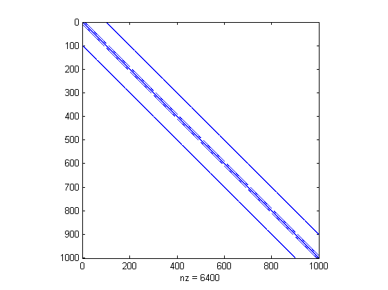
Figure 1: Structure of the matrix $A$ at time $T=1$.

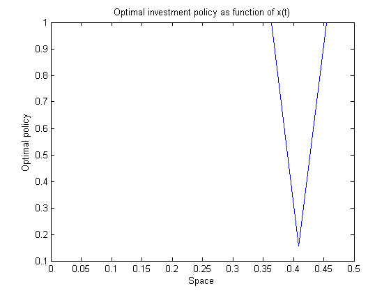
Figure 2: Optimal investment policy

at time $T=1$.

We compare the fitted finite volume and the finite difference method in Table 1

Time subdivision	$200$	$150$	$100$	$50$
Error of fitted finite volume method	4.65 E-01	6.31 E-01	8.63 E-01	1.30 E-00
Error of finite difference method	5.15 E-01	6.98 E-01	9.21 E-01	1.36 E-00

Table 1: Comparison of the implicit fitted finite volume method and implicit finite difference method. For the parameters, we have used $N_{1}=10$, $N_{2}=10$, $N_{3}=10$, $r_{1}=0.0449$, $\mu_{1}=0.0657$, $\mu_{2}=0.067$, $\mu_{3}=0.066$, $\sigma=0.2537$, $p=0.13$ and $T=1$.

Figure 4 shows the structure of the matrix $A$ and Figure 4 shows the optimal investment policy as function of $x$. The controller is the solution of (66). It is computed with the numerical procedure as outlined in Section 5.

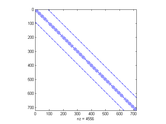
Figure 3: Structure of the matrix $A$ at time $T=1.5$.

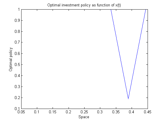
Figure 4: Optimal investment policy

at time $T=1.5$.

In Table 2, we have used $\Omega=[0,1/2]\times[0,1/4]\times[0,1/2]$ for computational domain with the following parameters $N_{1}=8$, $N_{2}=9$, $N_{1}=10$, $r_{1}=0.0449$, $r_{2}=0.0448/3$, $r_{3}=0.0447$, $\mu_{1}=0.0657$, $\mu_{2}=0.0656$, $\mu_{3}=0.0655$, $\sigma=0.2537$, $p=0.17$ and $T=1.5$.

Time subdivision	$200$	$150$	$100$	$50$
Error of the fitted finite volume method	2.24 E-01	2.30 E-01	3.99 E-01	5.97 E-01
Error of the finite difference method	2.40 E-01	3.18 E-01	4.12 E-01	5.99 E-01

Table 2: Comparison of the implicit fitted finite volume method and implicit finite difference method. For the parameters, we have used $N_{1}=8$, $N_{2}=9$, $N_{1}=10$, $r_{1}=0.0449$, $r_{2}=0.0448/3$, $r_{3}=0.0447$, $\mu_{1}=0.0657$, $\mu_{2}=0.0656$, $\mu_{3}=0.0655$, $\sigma=0.2537$, $p=0.17$ and $T=1.5$.

Table 1 and Table 2 display the numerical errors of finite volume method and finite difference method. By fitting the data from Table 1 and Table 2, we found that the convergence order in time $1$ for the fitted finite volume method and the finite difference method. From the two tables, we can observe a slight accuracy of the implicit fitted finite volume comparing to the implicit finite difference method, thanks to the fitted technique.

7 Conclusion

We have introduced a novel scheme based on finite volume method with fitted technique to solve high dimensional stochastic optimal control problems ($n\geq 3$). The optimization problem is solved at every time step using iterative method. We have shown that the system matrix of the resulting non linear system is an $M$-matrix and therefore the maximum principle is preserved for the discrete system obtained after the fitted finite volume spatial discretization. Numerical experiments are used to demonstrate the accuracy of the novel scheme comparing to the standard finite difference method.

8 Conflicts of interest/Competing interests

We have no conflicts of interest to declare.

References

- [1] Bénézet, C.; Chassagneux, J.-F. and Reisinger, C., A numerical scheme for the quantile hedging problem arXiv:1902.11228v1, (2019).
- [2] Henderson, V.; Kladívko, K.; Monoyios M. and Reisinger C. Executive stock option exercise with full and partial information on a drift change point. arXiv:1709.10141v4, (2020).
- [3] Zhu, Song-Ping, Ma, Guiyuan, An analytical solution for the HJB equation arising from the Merton problem. International Journal of Financial Engineering 05(01), 1850008 (26 pages), (2018).
- [4] Pfeiffer, Laurent; Two Approaches to Stochastic Optimal Control Problems with a Final-Time Expectation Constraint. Applied Mathematics & Optimization 77(2), 377-404, (2018).
- [5] Christelle Dleuna Nyoumbi and Antoine Tambue, A fitted finite volume method for stochastic optimal control problems in finance, AIMS Mathematics, 6(4), 3053–3079, (2021).
- [6] Valkov, R.: Fitted finite volume method for a generalized Black Scholes equation transformed on finite interval. Numerical Algorithms 65(1), 195–220 (2014).
- [7] Song, N., Ching, W.-K., Siu, T.-K., Yiu, C. K.-F.: On Optimal Cash Management under a Stochastic Volatility Model. East Asian Journal on Applied Mathematics 3 (2), 81–92 (2013).
- [8] Zhao, W., Tao, Z., Kong, T.: High order numerical schemes for second-order FBSDEs with applications to stochastic optimal control. Communications in Computational Physics 21(3), 808-834, (2017).
- [9] Rodriguez-Gonzalez, P. T., Rico-Ramirez, V., Rico-Martinez, R., Diwekar, U. M.: A new approach to solving stochastic optimal control problems. Mathematics 7, 1207, (2019)
- [10] Wang, S. A Novel fitted finite volume method for the Black Scholes equation governing option pricing. IMA J. Numer. Anal. 24, 699–720 (2004)
- [11] Hull, J., White, A.: The pricing of options on assets with stochastic volatilities. J.Finance 42(2), 281–300 (1987)
- [12] Holth, J.: Merton’s portfolio problem, constant fraction investment strategy and frequency of portfolio rebalancing. Master Thesis, University of Oslo, http://hdl.handle.net/10852/10798 (2011)
- [13] Gyöngy, I., Šiška, D. On finite difference approximations for normalized Bellman’s equations. Applied Mathematics and Optimization 60, Article number: 297 (2009)
- [14] Jakobsen, E.R.: On the rate of convergence of approximations schemes for Bellman equations associated with optimal stopping time problems. Mathematical Models and Methods in Applied Sciences 13 (05), 613–644 (2003)
- [15] Krylov, N.V.: On the rate of convergence of finite-difference approximations for Bellman’s equations with variable coefficients. Probability Theory and Related Fields 117, 1–16 (2000)
- [16] Krylov, N.V.: The rate of convergence of finite-difference approximations for Bellman’s equations with Lipschitz coefficients. Applied Mathematics and Optimization 52, 365–399 (2005)
- [17] Crandall, M.G., Lions, P.L. Viscosity solutions of Hamilton-Jacobi equations. Transactions of the American Mathematical Society 277(1), 1–42 (1983).
- [18] Crandall, M. G., Evans, L. C., Lions, P. L. Some properties of viscosity solutions of Hamilton-Jacobi equations. Transactions of the American Mathematical Society 282(2), 487–502 (1984)
- [19] Crandall, M.G. and Lions, P.L.: Two approximations of solutions of Hamilton-Jacobi equations. Mathematics of Computation 43, 1–19 (1984)
- [20] Pham, H.: Optimisation et contrôle stochastique appliqués à la finance. Mathématiques et applications, Springer-verlag New York (2000)
- [21] Wang, S., Gao F., Teo, K.L.: An upwind finite difference method for the approximation of viscosity solutions to Hamilton-Jacobi-Bellman equations. IMA Journal of Mathematical Control and Information 17, 167–178 (2000)
- [22] Krylov, N.V.: Approximating value functions for controlled degenerate diffusion processes by using piece-wise constant policies. Electronic Journal of Probability 4(2), 1–19 (1999)
- [23] Krylov, N. V.: Control of a solution of a stochastic integral equation. Th. Proba. Appl. 17, 406–446 (1972)
- [24] Crandall, M.G., Ishii, H., Lions, P.L.: User’s guide to viscosity solutions of second order partial differential equations. American Mathematical Society 27, 1–67 (1992)
- [25] Huang,C.-S., Wang, S., Teo, K.L.: On application of an alternating direction method to Hamilton-Jacobi-Bellman equations. Journal of Computational and Applied Mathematics 27, 153–166 (2004)
- [26] Barles, G., Souganidis, P.: Convergence of approximation schemes for fully nonlinear second-order equations. Asymptotic Anal. 4, 271–283 (1991)
- [27] Bonnans, J. F., Zidani, H.: Consistency of generalized finite difference schemes for the stochastic HJB equation. SIAM J. Numer. Anal. 41, 1008–1021 (2003)
- [28] Oberman, A. M.: Convergent difference schemes for degenerate elliptic and parabolic equations: Hamilton-Jacobi equations and free boundary problems. SIAM J. Numer. Anal. 44, 879–895 (2006)
- [29] Kushner, H. J.: Numerical methods for stochastic control problems in continuous time. SIAM J. Control Optim. 28, 999–1048 (1990)
- [30] Fleming, W. H., Soner, H. M.: Controlled Markov Processes and Viscosity Solutions, Stochastic Modelling and Applied Probability. Springer, New York 25 (2006)
- [31] Crandall, M. G., Lions, P. L.: Convergent difference schemes for nonlinear parabolic equations and mean curvature motion. Numer. Math. 75, 17–41 (1996)
- [32] Wilmott, P.: The Best of Wilmott 1: Incorporating the Quantitative Finance Review. John Wiley & Sons, (2005).
- [33] Kocan, M.: Approximation of viscosity solutions of elliptic partial differential equations on minimal grids. Numer. Math. 72, 73–92 (1995)
- [34] Peyrl, H., Herzog, F., Geering, H. P.: Numerical Solution of the Hamilton-Jacobi-Bellman Equation for Stochastic Optimal Control Problems. WSEAS Int. Conf. on Dynamical Systems and control, Venice, Italy, November 2-4, 489–497 (2005)
- [35] Huang, C.-S, Hung, C.-H, Wang, S.: On convergence of a Fitted Finite Volume Method for the Valuation of Options on Assets with Stochastic Volatilities. IMA J. Numer. Anal. 30, 1101–1120 (2010)
- [36] Huang, C.-S., Hung, C.-H., Wang, S.: A Fitted Finite Volume Method for the Valuation of Options on Assets with Stochastic Volatilities. Computing 77(3), 297–320 (2006)
- [37] Forsyth, P., Labahn, G.: Numerical Methods for Controlled Hamilton-Jacobi-Bellman PDEs in Finance. Journal of Computational Finance 11(2), 1–43 (2007)
- [38] Angermann, L. and Wang, S. Convergence of a fitted finite volume method for the penalized Black– Scholes equation governing European and American Option pricing, Numerische Mathematik, 106, 1–40 (2007).