\newsiamthm

claimClaim \newsiamremarkremarkRemark \newsiamremarkhypothesisHypothesis \newsiamthmproblemProblem \newsiamthmassumptionAssumption


\headersParareal Algorithms with Arbitrarily High-order Fine PropagatorsJiang Yang, Zhaoming Yuan and Zhi Zhou


Robust Convergence of Parareal Algorithms with Arbitrarily High-order Fine Propagators thanks: \fundingThe work of J. Yang is supported by National Natural Science Foundation of China (NSFC) Grant No. 11871264and the research of Z. Yuan and Z. Zhou is partially supported by Hong Kong RGC grant (No. 15304420).

Jiang Yang Department of Mathematics & SUSTech International Center for Mathematics, Southern University of Science and Technology, Shenzhen 518055, China. (yangj7sustech.edu.cn)    Zhaoming Yuan Department of Applied Mathematics, The Hong Kong Polytechnic University, Kowloon, Hong Kong. Department of Mathematics & SUSTech International Center for Mathematics, Southern University of Science and Technology, Shenzhen 518055, China. (zhaoming.yuan@connect.polyu.hk)    Zhi Zhou Department of Applied Mathematics, The Hong Kong Polytechnic University, Kowloon, Hong Kong. (zhizhou@polyu.edu.hk, zhizhou0125@gmail.com)
Abstract

The aim of this paper is to analyze the robust convergence of a class of parareal algorithms for solving parabolic problems. The coarse propagator is fixed to the backward Euler method and the fine propagator is a high-order single step integrator. Under some conditions on the fine propagator, we show that there exists some critical Jsubscript𝐽J_{*} such that the parareal solver converges linearly with a convergence rate near 0.30.30.3, provided that the ratio between the coarse time step and fine time step named J𝐽J satisfies JJ𝐽subscript𝐽J\geq J_{*}. The convergence is robust even if the problem data is nonsmooth and incompatible with boundary conditions. The qualified methods include all absolutely stable single step methods, whose stability function satisfies |r()|<1𝑟1|r(-\infty)|<1, and hence the fine propagator could be arbitrarily high-order. Moreover, we examine some popular high-order single step methods, e.g., two-, three- and four-stage Lobatto IIIC methods, and verify that the corresponding parareal algorithms converge linearly with a factor 0.310.310.31 and the threshold for these cases is J=2subscript𝐽2J_{*}=2. Intensive numerical examples are presented to support and complete our theoretical predictions.

keywords:
parareal algorithm, parabolic problems, arbitrarily high-order, single step integrator, convergence factor

{AMS}
Primary 65M12, 65M60; Secondary 65L06


1 Introduction

The main focus of this paper is to study the convergence of a class of parareal solver for the parabolic problems. Specifically, we let T>0,u0H,formulae-sequence𝑇0superscript𝑢0𝐻T>0,u^{0}\in H, and consider the initial value problem of seeking uC((0,T];D(A))C([0,T];H)𝑢𝐶0𝑇𝐷𝐴𝐶0𝑇𝐻u\in C((0,T];D(A))\cap C([0,T];H) satisfying

(1) {u(t)+Au(t)=f(t),0<t<T,u(0)=u0,\left\{\begin{aligned} &u^{\prime}(t)+Au(t)=f(t),\quad 0<t<T,\\ &u(0)=u^{0},\end{aligned}\right.

where A𝐴A is a positive definite, selfadjoint, linear operator with a compact inverse, defined in Hilbert space (H,(,))𝐻(H,(\cdot,\cdot)) with domain D(A)𝐷𝐴D(A) dense in H𝐻H. Here u0Hsuperscript𝑢0𝐻u^{0}\in H is a given initial condition and f:[0,T]H:𝑓0𝑇𝐻f:[0,T]\to H is a given forcing term. Throughout the paper, \|\cdot\| denotes the norm of the space H𝐻H.

Parallel-in-time (PinT) methods, dating back to the work of Nievergelt in 1964 [23], have attracted a lot of interest in the last several decades. The parareal method, introduced in 2001 [20], is perhaps one of the most popular PinT algorithms. This method is relatively simple to implement, and can be employed for any single step integrators. In recent years, the parareal algorithm and some relevant algorithms, have been applied in many fields, such as turbulent plasma [25, 26], structural (fluid) dynamics [9, 12], molecular dynamics [4], optimal control [21, 22] Volterra integral equations and fractional models [19, 34], etc. We refer the interested reader to survey papers [13, 24] and references therein.

The parareal algorithm is defined by using two time propagators, 𝒢𝒢\mathcal{G} and \mathcal{F}, associated with the large step size ΔTΔ𝑇\Delta T and the small step size ΔtΔ𝑡\Delta t respectively, where we assume that the ratio J=ΔT/Δt𝐽Δ𝑇Δ𝑡J=\Delta T/\Delta t is an integer greater than 111. The fine time propagator \mathcal{F} is operated with small step size ΔtΔ𝑡\Delta t in each coarse sub-interval parallelly, after which the coarse time propagator 𝒢𝒢\mathcal{G} is operated with large step size ΔTΔ𝑇\Delta T sequentially for corrections. In general, the coarse propagator 𝒢𝒢\mathcal{G} is assumed to be much cheaper than the fine propagator \mathcal{F}. Therefore, throughout this paper, we fix 𝒢𝒢\mathcal{G} to the backward-Euler method and study the choices of \mathcal{F}. Then a natural question arises related to convergence of the parareal algorithm. For parabolic type problems, in the pioneer work [5], Bal proved a fast convergence of the parareal method with a strongly stable coarse propagator and the exact fine propagator, provided some regularity assumptions on the problem data. The analysis works for both linear and nonlinear problems. This convergence behavior is clearly observed in numerical experiments, see e.g. Figure 5.1. However, without those regularity assumptions, the convergence observed from the empirical experiments will be much slower than expected, cf. Figure 5.2.

This interesting phenomenon motivates the current work, where we aim to study the convergence of parareal algorithm which is expected to be robust in the case of nonsmooth / incompatible problem data, that is related to various applications, e.g., optimal control, inverse problems, and stochastic models. There have existed some case studies. In [22], Mathew, Sarkis and Schaerer considered the backward Euler method as the fine propagator and proved the robust convergence of the parareal algorithm with a convergence factor 0.2980.2980.298 (for all J2𝐽2J\geq 2); see also [14, 29] for some related discussion. In [32], Wu showed that the convergence factors for the second-order diagonal implicit Runge–Kutta method and a single step TR/BDF2 method (i.e., the ode23tb solver for ODEs in MATLAB) are 0.3160.3160.316 (with J2𝐽2J\geq 2) and 0.3330.3330.333 (with J2𝐽2J\geq 2), respectively. These error bounds might be slightly improved by increasing Jsubscript𝐽J_{*}. See also [33] for the analysis for a third-order diagonal implicit Runge–Kutta method with a convergence factor 0.3330.3330.333 (J=4subscript𝐽4J_{*}=4). For fourth-order Gauss–Runge–Kutta integrator, in [33] Wu and Zhou showed that the threshold depends on both the largest eigenvalue of operator A𝐴A and the step size ΔtΔ𝑡\Delta t. Note that the eigenvalues of A𝐴A may approach infinity, e.g. A=Δ𝐴ΔA=-\Delta with homogeneous boundary conditions. Therefore, this kind of integrators might not be suitable for the parareal algorithm.

Then a natural question arises: in what case there exists a threshold J>0subscript𝐽0J_{*}>0 (independent of step sizes ΔTΔ𝑇\Delta T, ΔtΔ𝑡\Delta t, terminal time T𝑇T, problem data u0superscript𝑢0u^{0} and f𝑓f, as well as the distribution of spectrum of the elliptic operator A𝐴A), such that for any JJ𝐽subscript𝐽J\geq J_{*}, the parareal algorithm for solving the parabolic equation (1) converges robustly? Our study provides a positive answer to this question: if the fine propagator is strongly stable, in sense that the stability function satisfies |r()|[0,1)𝑟01|r(-\infty)|\in[0,1), then there must exist such a positive threshold Jsubscript𝐽J_{*} so that for all JJ𝐽subscript𝐽J\geq J_{*} the parareal algorithm converges linearly with convergence factor close to 0.30.30.3. The convergence is robust even if the initial data is nonsmooth or incompatible with boundary conditions. Noting that all L-stable Runge–Kutta schemes satisfy that condition, so the fine propagator can be arbitrarily high-order. As examples, we analyzed three popular L-stable schemes, i.e., two-, three-, four-stage Lobatto IIIC schemes. We show that for all these cases the parareal algorithm converges linearly with factor less than 0.310.310.31 and J=2subscript𝐽2J_{*}=2. Our theoretical results are fully supported by numerical experiments.

The rest of the paper is organized as follows. In Section 2, we introduce singe step integrators and parareal algorithms for solving the parabolic problem. Then we show the convergence of the algorithm in Section 3 by using the spectrum decomposition. Moreover, in Section 4, we present case studies on three popular L-stable Runge–Kutta schemes, and show a sharper estimate for the threshold Jsubscript𝐽J_{*}. Finally, in Section 5, we present some numerical results to illustrate and complement the theoretical analysis.

2 Single step methods and parareal algorithm

In this section, we present the basic setting of the single step time stepping methods for solving the parabolic equation (1) and the parareal algorithm. See more detailed discussion in the monograph [30, Chapter 7-9] and the comprehensive survey paper [13].

2.1 Single step integrators for solving parabolic equations

To begin with, we consider the time discretization for the parabolic equation (1). We split the interval (0,T)0𝑇(0,T) into N𝑁N subintervals with the uniform mesh size Δt=T/NΔ𝑡𝑇𝑁{\Delta t}=T/N, and set tn=nΔtsubscript𝑡𝑛𝑛Δ𝑡t_{n}=n{\Delta t}, n=0,1,,N𝑛01𝑁n=0,1,\ldots,N. Then a framework of a single step scheme approximating u(tn)𝑢subscript𝑡𝑛u(t_{n}) reads:

(2) un+1=r(ΔtA)un+Δti=1mpi(ΔtA)f(tn+ciΔt),for all0nN1,formulae-sequencesuperscript𝑢𝑛1𝑟Δ𝑡𝐴superscript𝑢𝑛Δ𝑡superscriptsubscript𝑖1𝑚subscript𝑝𝑖Δ𝑡𝐴𝑓subscript𝑡𝑛subscript𝑐𝑖Δ𝑡for all0𝑛𝑁1u^{n+1}=r(-{\Delta t}A)u^{n}+{\Delta t}\sum_{i=1}^{m}p_{i}(-{\Delta t}A)f(t_{n}+c_{i}\Delta t),\quad\text{for all}~{}0\leq n\leq N-1,

Here, r(λ)𝑟𝜆r(\lambda) and {pi(λ)}i=1msubscriptsuperscriptsubscript𝑝𝑖𝜆𝑚𝑖1\{p_{i}(\lambda)\}^{m}_{i=1} are rational functions and cisubscript𝑐𝑖c_{i} are distinct real numbers in [0,1]01[0,1]. Throughout the paper, we assume that the scheme (2) satisfies the following assumptions.

  • (P1)

    |r(λ)|<1𝑟𝜆1|r(-\lambda)|<1 and |pi(λ)|csubscript𝑝𝑖𝜆𝑐|p_{i}(-\lambda)|\leq c, for all i=1,,m𝑖1𝑚i=1,\ldots,m, uniformly in ΔtΔ𝑡{\Delta t} and λ>0𝜆0\lambda>0. Besides, the numerator of pi(λ)subscript𝑝𝑖𝜆p_{i}(\lambda) is of lower degree than its denominator.

  • (P2)

    The time stepping scheme (2) is accurate of order $q$ in sense that

    $$r(-\lambda)=e^{-\lambda}+O(\lambda^{q+1}),\quad\text{as}~{}\lambda\rightarrow 0.$$

    and for $0\leq j\leq q$

    $$\sum_{i=1}^{m}c_{i}^{j}p_{i}(-\lambda)-\frac{j!}{(-\lambda)^{j+1}}\Big{(}e^{-\lambda}-\sum_{\ell=0}^{j}\frac{(-\lambda)^{\ell}}{\ell!}\Big{)}=O(\lambda^{q-j}),\quad\text{as}~{}\lambda\rightarrow 0.$$
  • (P3)

    The rational function $r(\lambda)$ is strongly stable in sense that $|r(-\infty)|<1$.

Remark 2.1.

Condition (P3) is essential for the convergence of parareal iteration. If |r()|=1𝑟1|r(\infty)|=1, e.g., Crank-Nicolson method and implicit Runge-Kutta methods of Gauss type, the parareal method converges only if the eigenvalues of A𝐴A is bounded from above (which is not true for parabolic equations) and the ratio between the coarse step size and the fine step size is sufficiently large (depending on the upper bound of eigenvalues of A𝐴A). Besides, this condition is also important in case that problem data is nonsmooth, e.g., u0Hsuperscript𝑢0𝐻u^{0}\in H. Time stepping schemes violating this condition may lose the optimal convergence rate in the nonsmooth data case [30, Chapter 8].

Practically, it is convenient to choose $p_{i}(\lambda)$ that share the same denominator of $r(\lambda)$:

$$r(\lambda)=\frac{a_{0}(\lambda)}{g(\lambda)},\quad\text{and}\quad p_{i}(\lambda)=\frac{a_{i}(\lambda)}{g(\lambda)},\quad\text{for}~{}i=1,2,\ldots,m,$$

where ai(λ)subscript𝑎𝑖𝜆a_{i}(\lambda) and g(λ)𝑔𝜆g(\lambda) are polynomials. Then the integrator (2) could be written as

$$g(-{\Delta t}A)u^{n+1}=a_{0}(-{\Delta t}A)u^{n}+{\Delta t}\sum_{i=1}^{m}a_{i}(-{\Delta t}A)f(t_{n}+c_{i}\Delta t),\quad\text{for all}~{}1\leq n\leq N.$$

See e.g. [30, pp. 131] for the construction of such rational functions satisfying (P1)-(P3).

Under those conditions, there holds the following error estimate for the time stepping scheme (2). The proof is given in [30, Theorems 7.2 and 8.3].

Lemma 2.2.

Suppose that the Conditions (P1)-(P3) are fulfilled. Let u(t)𝑢𝑡u(t) be the solution to parabolic equation (1), and unsuperscript𝑢𝑛u^{n} be the solution to the time stepping scheme (2). Then there holds

$$\|u^{n}-u(t_{n})\|\leq c\,(\Delta t)^{q}\Big{(}t_{n}^{-q}\|u^{0}\|+t_{n}\sum_{\ell=0}^{q-1}\sup_{s\leq t_{n}}\|A^{q-\ell}f^{(\ell)}(s)\|+\int_{0}^{t_{n}}\|f^{(q)}(s)\|\,{\mathrm{d}}s\Big{)},$$

provided that $v\in H$, $f^{(\ell)}\in C([0,T];\text{Dom}(A^{q-\ell})$ with $0\leq\ell\leq q-1$ and $f^{(q)}\in L^{1}(0,T;H)$ for all $\ell<q$.

Remark 2.3.

Lemma 2.2 indicates that, under Conditions (P1)-(P3), the solution of the time stepping scheme (2) converges to the exact solution with order q𝑞q provided that the source term f𝑓f and initial condition u0subscript𝑢0u_{0} satisfy certain compatibility conditions. For example, if we consider the parabolic equation where A=Δ𝐴ΔA=-\Delta with homogeneous Dirichlet boundary condition, it requires (Δ)f(q)=0superscriptΔsuperscript𝑓𝑞0(-\Delta)^{\ell}f^{(q-\ell)}=0 on the boundary ΩΩ\partial\Omega for 0q0𝑞0\leq\ell\leq q. In order to avoid the restrictive compatibility conditions, we shall assume that the time discretization scheme (2) is strictly accurate of order q𝑞q in sense that

$$\sum_{i=1}^{m}c_{i}^{j}p_{i}(-\lambda)-\frac{j!}{(-\lambda)^{j+1}}\Big{(}r(-\lambda)-\sum_{\ell=0}^{j}\frac{(-\lambda)^{\ell}}{\ell!}\Big{)}=0,\quad\text{for all}~{}0\leq j\leq q-1.$$

It is well-known that a single step method with a given m+𝑚superscriptm\in\mathbb{Z}^{+} could be accurate of order 2m2𝑚2m (Gauss–Legendre method) [11, Section 2.2], but at most strictly accurate of order m+1𝑚1m+1 [6, Lemma 5].

Remark 2.4.

The error estimate in Lemma 2.2 could be slightly improved if the time integrator is L-stable, i.e. $r(-\infty)=0$; see e.g., [30, Theorem 7.2].

2.2 Parareal algorithm

Next, we state the parareal solver for the single step scheme (2). Let ΔT=JΔtΔ𝑇𝐽Δ𝑡\Delta T=J\Delta t, with a positive integer J2𝐽2J\geq 2, be the coarse step size. Without loss of generality, we assume that Nc=T/ΔTsubscript𝑁𝑐𝑇Δ𝑇N_{c}=T/\Delta T is an integer, and let Tn=nΔTsubscript𝑇𝑛𝑛Δ𝑇T_{n}=n\Delta T Then, two numerical propagators 𝒢𝒢{\mathcal{G}} and {\mathcal{F}} are assigned to the coarse and fine time grids, where 𝒢𝒢{\mathcal{G}} is usually a low-order and inexpensive numerical method (such as backward Euler scheme), and {\mathcal{F}} is given by the single step integrator (2). Specifically, for vH𝑣𝐻v\in H and fC([0,T];H)𝑓𝐶0𝑇𝐻f\in C([0,T];H), letting I𝐼I denote the identity operator, we define the coarse and finer propagator as

$${\mathcal{G}}(T_{n},\Delta T,v,f)=(I+\Delta TA)^{-1}(v+\Delta Tf(T_{n})).$$

and

$${\mathcal{F}}(t_{n},\Delta t,v,f)=r(-{\Delta t}A)v+{\Delta t}\sum_{i=1}^{m}p_{i}(-{\Delta t}A)f(t_{n}+c_{i}\Delta t).$$

respectively. Then, the parareal solver is described in Algorithm 1.

Algorithm 1 Parareal solver for the single step scheme (2).
1:  Initialization: Compute U0n+1=𝒢(Tn,ΔT,U0n+1,f)superscriptsubscript𝑈0𝑛1𝒢subscript𝑇𝑛Δ𝑇superscriptsubscript𝑈0𝑛1𝑓U_{0}^{n+1}={\mathcal{G}}(T_{n},\Delta T,U_{0}^{n+1},f) with U00=u0superscriptsubscript𝑈00superscript𝑢0U_{0}^{0}=u^{0}, n=0,1,,Nc1𝑛01subscript𝑁𝑐1n=0,1,...,N_{c}-1;
2:  for $k=0,1,\ldots,K$ do
3:     Step 1: On each subinterval $[T_{n},T_{n}+1]$, sequetially compute for $j=1,2,\dots,J-1$
$$\widetilde{U}^{n,j+1}={\mathcal{F}}(T_{n}+j\Delta t,\Delta t,\widetilde{U}^{n,j},f),$$
with initial value U~n,0=Uknsuperscript~𝑈𝑛0superscriptsubscript𝑈𝑘𝑛\widetilde{U}^{n,0}=U_{k}^{n}. Let U~n+1=U~n,Jsuperscript~𝑈𝑛1superscript~𝑈𝑛𝐽\widetilde{U}^{n+1}=\widetilde{U}^{n,J}.
4:     Step 2: Perform sequential corrections: find $U_{k+1}^{n+1}$
$$U_{k+1}^{n+1}={\mathcal{G}}(T_{n},\Delta T,U_{k+1}^{n},f)+\widetilde{U}^{n+1}-{\mathcal{G}}(T_{n},\Delta T,U_{k}^{n},f)$$
with $U_{k+1}^{0}=u^{0}$, for $n=0,1,...,N_{c}-1$;
5:     Step 3: If $\{U_{k+1}^{n}\}_{n=1}^{N_{c}}$ satisfies the stopping criterion, terminate the iteration; otherwise go to Step 1.
6:  end for

The aim of this paper is to show that the iterative solution Uknsuperscriptsubscript𝑈𝑘𝑛U_{k}^{n}, generated by the parareal algorithm, linearly converges to the exact time stepping solution unJsuperscript𝑢𝑛𝐽u^{nJ} of the single step integrator (2) with fine time step ΔtΔ𝑡\Delta t, i.e.,

(3) max1nNUknunJcγk,subscript1𝑛𝑁normsuperscriptsubscript𝑈𝑘𝑛superscript𝑢𝑛𝐽𝑐superscript𝛾𝑘\max_{1\leq n\leq N}\|U_{k}^{n}-u^{nJ}\|\leq c\,\gamma^{k},

with some convergence factor γ𝛾\gamma strictly smaller than 111. We shall prove that there exists a positive threshold Jsubscript𝐽J_{*}, independent of ΔTΔ𝑇\Delta T, ΔtΔ𝑡\Delta t and the upper bound of spectrum of A𝐴A, such that if JJ𝐽subscript𝐽J\geq J_{*}, then (3) is true with γ𝛾\gamma close to 0.30.30.3, under conditions (P1)-(P3).

3 Convergence analysis

Next, we briefly test the convergence factor of parareal iteration. Taking comparision with the exact time stepping solution in (2), we arrive at

Uk+1n+1u(n+1)Jsuperscriptsubscript𝑈𝑘1𝑛1superscript𝑢𝑛1𝐽\displaystyle U_{k+1}^{n+1}-u^{(n+1)J} =(I+ΔTA)1[(Uk+1nunJ)(UknunJ)]absentsuperscript𝐼Δ𝑇𝐴1delimited-[]superscriptsubscript𝑈𝑘1𝑛superscript𝑢𝑛𝐽superscriptsubscript𝑈𝑘𝑛superscript𝑢𝑛𝐽\displaystyle=(I+\Delta TA)^{-1}\Big{[}(U_{k+1}^{n}-u^{nJ})-(U_{k}^{n}-u^{nJ})\Big{]}
$\displaystyle\quad+F(T_{n}+(J-1)\Delta t,\Delta t,\widetilde{U}^{n,J-1},f)-F(T_{n}+(J-1)\Delta t,\Delta t,u^{nJ-1},f))$
$\displaystyle=(I+\Delta TA)^{-1}\Big{[}(U_{k+1}^{n}-u^{nJ})-(U_{k}^{n}-u^{nJ})\Big{]}+r(-\Delta tA)(\widetilde{U}^{n,J-1}-u^{(n+1)J-1})$
$\displaystyle=\cdots$
$\displaystyle=(I+\Delta TA)^{-1}\Big{[}(U_{k+1}^{n}-u^{nJ})-(U_{k}^{n}-u^{nJ})\Big{]}+r(-\Delta tA)^{J}(\widetilde{U}^{n,0}-u^{nJ})$
$\displaystyle=(I+\Delta TA)^{-1}\Big{[}(U_{k+1}^{n}-u^{nJ})-(U_{k}^{n}-u^{nJ})\Big{]}+r(-\Delta tA)^{J}(U_{k}^{n}-u^{nJ}),$

For the sake of simplicity, we define $E_{k}^{n}=U_{k}^{n}-u^{nJ}$ and rewrite the above equation as

$$E_{k+1}^{n+1}=(I+\Delta TA)^{-1}(E_{k+1}^{n}-E_{k}^{n})+r(-\Delta tA)^{J}E_{k}^{n}$$

Recall that the operator A𝐴A is a positive definite, selfadjoint, linear operator with a compact inverse, defined in Hilbert space (H,(,))𝐻(H,(\cdot,\cdot)). Then by the spectral theory, A𝐴A has positive eigenvalues {λj}j=1superscriptsubscriptsubscript𝜆𝑗𝑗1\{\lambda_{j}\}_{j=1}^{\infty}, where 0<λ1λ20subscript𝜆1subscript𝜆20<\lambda_{1}\leq\lambda_{2}\leq\ldots and λjsubscript𝜆𝑗\lambda_{j}\rightarrow\infty, and the corresponding eigenfunctions {ϕj}j=1superscriptsubscriptsubscriptitalic-ϕ𝑗𝑗1\{\phi_{j}\}_{j=1}^{\infty} form an orthonormal basis of the Hilbert space H𝐻H. Then, letting ek,jn=(Ekn,ϕj)superscriptsubscript𝑒𝑘𝑗𝑛superscriptsubscript𝐸𝑘𝑛subscriptitalic-ϕ𝑗e_{k,j}^{n}=(E_{k}^{n},\phi_{j}), by means of spectrum decomposition, we derive

$\displaystyle e_{k+1,j}^{n+1}=\frac{e_{k+1,j}^{n}-e_{k,j}^{n}}{1+\Delta T\lambda_{j}}+r(-\Delta t\lambda_{j})^{J}e_{k,j}^{n}.$

By letting $d_{j}=\Delta T\lambda_{j}$, we have

$\displaystyle e_{k+1,j}^{n+1}\leq(1+d_{j})^{-1}e_{k+1,j}^{n}+(r(-d_{j}/J)^{J}-(1+d_{j})^{-1})e_{k,j}^{n}.$

We apply the recursion and use the fact that $e_{k+1,j}^{0}=0$, and hence obtain

ek+1,jn+1=superscriptsubscript𝑒𝑘1𝑗𝑛1absent\displaystyle e_{k+1,j}^{n+1}= (r(dj/J)J(1+dj)1)ek,jn+(1+dj)1ek+1,jn𝑟superscriptsubscript𝑑𝑗𝐽𝐽superscript1subscript𝑑𝑗1superscriptsubscript𝑒𝑘𝑗𝑛superscript1subscript𝑑𝑗1superscriptsubscript𝑒𝑘1𝑗𝑛\displaystyle(r(-d_{j}/J)^{J}-(1+d_{j})^{-1})e_{k,j}^{n}+(1+d_{j})^{-1}e_{k+1,j}^{n}
=\displaystyle= (r(dj/J)J(1+dj)1)(ek,jn+(1+dj)1ek,jn1)+(1+dj)2ek+1,jn1𝑟superscriptsubscript𝑑𝑗𝐽𝐽superscript1subscript𝑑𝑗1superscriptsubscript𝑒𝑘𝑗𝑛superscript1subscript𝑑𝑗1superscriptsubscript𝑒𝑘𝑗𝑛1superscript1subscript𝑑𝑗2superscriptsubscript𝑒𝑘1𝑗𝑛1\displaystyle(r(-d_{j}/J)^{J}-(1+d_{j})^{-1})\Big{(}e_{k,j}^{n}+(1+d_{j})^{-1}e_{k,j}^{n-1}\Big{)}+(1+d_{j})^{-2}e_{k+1,j}^{n-1}
=\displaystyle= \displaystyle\dots
=\displaystyle= (r(dj/J)J(1+dj)1)(ek,jn+(1+dj)1ek,jn1++(1+dj)(n1)ek,j1).𝑟superscriptsubscript𝑑𝑗𝐽𝐽superscript1subscript𝑑𝑗1superscriptsubscript𝑒𝑘𝑗𝑛superscript1subscript𝑑𝑗1superscriptsubscript𝑒𝑘𝑗𝑛1superscript1subscript𝑑𝑗𝑛1superscriptsubscript𝑒𝑘𝑗1\displaystyle(r(-d_{j}/J)^{J}-(1+d_{j})^{-1})\Big{(}e_{k,j}^{n}+(1+d_{j})^{-1}e_{k,j}^{n-1}+\dots+(1+d_{j})^{-(n-1)}e_{k,j}^{1}\Big{)}.

Now taking the absolute value on the both sides yields

(4) |ek+1,jn+1|superscriptsubscript𝑒𝑘1𝑗𝑛1absent\displaystyle|e_{k+1,j}^{n+1}|\leq |r(dj/J)J(1+dj)1|(1+(1+dj)1++(1+dj)(n1))max1nN|ek,jn|𝑟superscriptsubscript𝑑𝑗𝐽𝐽superscript1subscript𝑑𝑗11superscript1subscript𝑑𝑗1superscript1subscript𝑑𝑗𝑛1subscript1𝑛𝑁superscriptsubscript𝑒𝑘𝑗𝑛\displaystyle|r(-d_{j}/J)^{J}-(1+d_{j})^{-1}|\cdot(1+(1+d_{j})^{-1}+\dots+(1+d_{j})^{-(n-1)})\max_{1\leq n\leq N}{|e_{k,j}^{n}|}
\displaystyle\leq |r(dj/J)J(1+dj)1|1(1+dj)1max1nN|ek,jn|𝑟superscriptsubscript𝑑𝑗𝐽𝐽superscript1subscript𝑑𝑗11superscript1subscript𝑑𝑗1subscript1𝑛𝑁superscriptsubscript𝑒𝑘𝑗𝑛\displaystyle\frac{|r(-d_{j}/J)^{J}-(1+d_{j})^{-1}|}{1-(1+d_{j})^{-1}}\max_{1\leq n\leq N}{|e_{k,j}^{n}|}
=\displaystyle= |(1+dj)r(dj/J)J1dj|max1nN|ek,jn|1subscript𝑑𝑗𝑟superscriptsubscript𝑑𝑗𝐽𝐽1subscript𝑑𝑗subscript1𝑛𝑁superscriptsubscript𝑒𝑘𝑗𝑛\displaystyle\left|\frac{(1+d_{j})r(-d_{j}/J)^{J}-1}{d_{j}}\right|\max_{1\leq n\leq N}{|e_{k,j}^{n}|}
\displaystyle\leq sups(0,)|(1+s)r(s/J)J1s|max1nN|ek,jn|.subscriptsupremum𝑠01𝑠𝑟superscript𝑠𝐽𝐽1𝑠subscript1𝑛𝑁superscriptsubscript𝑒𝑘𝑗𝑛\displaystyle\sup_{s\in(0,\infty)}\left|\frac{(1+s)r(-s/J)^{J}-1}{s}\right|\max_{1\leq n\leq N}{|e_{k,j}^{n}|}.

If the the leading factor is strictly smaller than one, i.e.,

(5) sups(0,)|(1+s)r(s/J)J1s|γ<1,subscriptsupremum𝑠01𝑠𝑟superscript𝑠𝐽𝐽1𝑠𝛾1\sup_{s\in(0,\infty)}\left|\frac{(1+s)r(-s/J)^{J}-1}{s}\right|\leq\gamma<1,

then eknsuperscriptsubscript𝑒𝑘𝑛e_{k}^{n} converges to zero linearly with a factor (smaller than) γ𝛾\gamma, and hence the parareal iteration converges linearly to the time stepping solution (2) in sense of (3).

Our convergence analysis in this and next sections heavily depend on the constant $\kappa_{\alpha}$ defined by

(6) κα:=sups(0,)|(1+s)eαs1s|,forα[0,2].formulae-sequenceassignsubscript𝜅𝛼subscriptsupremum𝑠01𝑠superscript𝑒𝛼𝑠1𝑠for𝛼02\kappa_{\alpha}:=\sup_{s\in(0,\infty)}\left|\frac{(1+s)e^{-\alpha s}-1}{s}\right|,\qquad\text{for}~{}~{}\alpha\in[0,2].

To begin with, we establish an simple upper bound for the constant $\kappa_{\alpha}$.

Lemma 3.1.

Let α[0,2]𝛼02\alpha\in[0,2], and καsubscript𝜅𝛼\kappa_{\alpha} be the constant defined in (6). Then there holds

κα{eα2,α[1,2];max(eα2,1α),α[0,1).subscript𝜅𝛼casessuperscript𝑒𝛼2𝛼12superscript𝑒𝛼21𝛼𝛼01\begin{split}\kappa_{\alpha}\leq\begin{cases}e^{\alpha-2},\quad&\alpha\in[1,2];\\ \max(e^{\alpha-2},1-\alpha),&\alpha\in[0,1).\end{cases}\end{split}

Proof 3.2.

First of all, we show the claim that

(7) (1+s)eαs1seα2.1𝑠superscript𝑒𝛼𝑠1𝑠superscript𝑒𝛼2\frac{(1+s)e^{-\alpha s}-1}{s}\geq-e^{\alpha-2}.

To this end, we define the auxiliary function

$$g(s)=(1+s)e^{-\alpha s}+e^{\alpha-2}s.$$

Then a simple computation yields

$$g^{\prime}(s)=(1-\alpha-\alpha s)e^{-\alpha s}+e^{\alpha-2}\quad\text{and}\quad g^{\prime\prime}(s)=(\alpha^{2}+\alpha^{2}s-2\alpha)e^{-\alpha s}.$$

It is easy to observe that g′′(s)superscript𝑔′′𝑠g^{\prime\prime}(s) admits a single root at s=(2α)/α𝑠2𝛼𝛼s=(2-\alpha)/\alpha, and

$$g^{\prime}(x)\geq g^{\prime}((2-\alpha)/\alpha)=0.$$

Therefore g(s)𝑔𝑠g(s) is increasing in [0,)0[0,\infty). As a result, g(s)g(0)=1𝑔𝑠𝑔01g(s)\geq g(0)=1, and hence

$${(1+s)e^{-\alpha s}-1}\geq-e^{\alpha-2}{s}\qquad\forall~{}~{}s\geq 0,$$

which implies (7). Moreover, for α1𝛼1\alpha\geq 1, we observe that

$$1+s\leq e^{s}\leq e^{\alpha s}\qquad\forall s\geq 0,$$

which immediately leads to (1+s)eαs101𝑠superscript𝑒𝛼𝑠10(1+s)e^{-\alpha s}-1\leq 0 for all s0𝑠0s\geq 0. This completes the proof for the desired results in case that α[1,2]𝛼12\alpha\in[1,2].

Now we turn to the case that α[0,1)𝛼01\alpha\in[0,1). Let κα=max{eα2,1α}superscriptsubscript𝜅𝛼superscript𝑒𝛼21𝛼\kappa_{\alpha}^{*}=\max\{e^{\alpha-2},1-\alpha\} and define

$$g(x)=(1+s)e^{-\alpha s}-\kappa_{\alpha}^{*}s.$$

Then the simple computation yields

$$g^{\prime}(s)=(1-\alpha-\alpha s)e^{-\alpha s}-\kappa_{\alpha}^{*}\quad\text{and}\quad g^{\prime\prime}(s)=(\alpha^{2}+\alpha^{2}s-2\alpha)e^{-\alpha s}.$$

Noting that g(0)=1ακα0superscript𝑔01𝛼superscriptsubscript𝜅𝛼0g^{\prime}(0)=1-\alpha-\kappa_{\alpha}^{*}\leq 0, g()=κα<0superscript𝑔superscriptsubscript𝜅𝛼0g^{\prime}(\infty)=-\kappa_{\alpha}^{*}<0 and g((2α)/α)0superscript𝑔2𝛼𝛼0g^{\prime}((2-\alpha)/\alpha)\leq 0. These imply g(s)0superscript𝑔𝑠0g^{\prime}(s)\leq 0 and hence g𝑔g is decreasing function in [0,)0[0,\infty). Therefore g(s)g(0)=1𝑔𝑠𝑔01g(s)\leq g(0)=1, which further implies

$$(1+s)e^{-\alpha s}-\kappa_{\alpha}^{*}s\leq 1.$$

This leads to the desired assertion for the case that $\alpha\in[0,1)$.

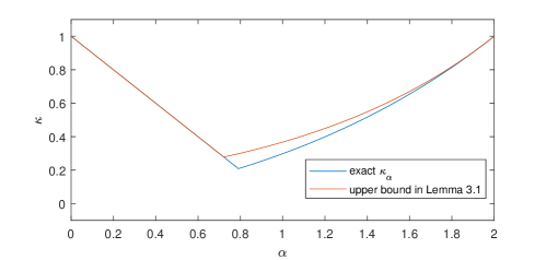
Lemma 3.1 only provides a rough upper bound for καsubscript𝜅𝛼\kappa_{\alpha}. In fact, for a fixed α𝛼\alpha we can further improve the upper bound via a more careful computation. In Figure 3.1, we numerically compute the constant καsubscript𝜅𝛼\kappa_{\alpha} for α[0,2]𝛼02\alpha\in[0,2] and plot those values.

Refer to caption
Figure 3.1: Plot of $\kappa_{\alpha}$ defined in lemma 3.1.

The next lemma provides a sharper estimate for $\kappa_{1}$.

Lemma 3.3.

Let $\kappa_{\alpha}$ be the constant defined in (6). Then $\kappa_{1}\approx 0.2984$.

Proof 3.4.

To show the sharp estimate, we note that for g(s)=1(1+s)es𝑔𝑠11𝑠superscript𝑒𝑠g(s)=1-(1+s)e^{-s}, there holds g(s)=ses0superscript𝑔𝑠𝑠superscript𝑒𝑠0g^{\prime}(s)=se^{-s}\geq 0 and g(0)=1𝑔01g(0)=1. Therefore g(s)0𝑔𝑠0g(s)\geq 0 for all s(0,)𝑠0s\in(0,\infty). This further implies ψ(s)=(1(1+s)es)/s0𝜓𝑠11𝑠superscript𝑒𝑠𝑠0\psi(s)=(1-(1+s)e^{-s})/s\geq 0 for s(0,)𝑠0s\in(0,\infty).

Meanwhile, we note that

$$\varphi(s):=s^{2}e^{s}\psi^{\prime}(s)=s^{2}+s+1-e^{s}.$$

It is easy to verify that φ(s)𝜑𝑠\varphi(s) has a unique root, denoted by ssubscript𝑠s_{*}, in (0,)0(0,\infty), so does ψ(s)superscript𝜓𝑠\psi^{\prime}(s). Therefore, κ1=f(s)subscript𝜅1𝑓subscript𝑠\kappa_{1}=f(s_{*}). Using the Newton’s algorithm, we find s1.793subscript𝑠1.793s_{*}\approx 1.793 and hence κ10.2984subscript𝜅10.2984\kappa_{1}\approx 0.2984.

Now we state our main theorem which verifies the desired result (5) with $\gamma\approx 0.3$.

Theorem 3.5.

Let conditions (P1)-(P3) hold valid. Then there exists a threshold J>0subscript𝐽0J_{*}>0 such that for all JJ𝐽subscript𝐽J\geq J_{*}

$$\sup_{s\in(0,\infty)}\left|\frac{(1+s)r(-s/J)^{J}-1}{s}\right|\leq 0.3,$$

Proof 3.6.

First of all, we aim to show that

(8) limJsups0(1+s)s|r(s/J)Jes|=0.subscript𝐽subscriptsupremum𝑠01𝑠𝑠𝑟superscript𝑠𝐽𝐽superscript𝑒𝑠0\lim_{J\rightarrow\infty}\sup_{s\geq 0}\frac{(1+s)}{s}\left|r(-s/J)^{J}-e^{-s}\right|=0.

For a given δ>0𝛿0\delta>0, for any s>δ𝑠𝛿s>\delta, it is obvious that (1+s)/s1𝑠𝑠(1+s)/s is bounded by a constant C(δ)𝐶𝛿C(\delta). Meanwhile, note that conditions (P1)-(P3) are fullfilled. Then by means of the nonsmooth data error estimate [30, Theorem 7.2], there holds

$$\left|r(-s/J)^{J}-e^{-s}\right|\leq cJ^{-q},$$

where c𝑐c is independent of s𝑠s. Then we derive

$$\lim_{J\rightarrow\infty}\sup_{s>\delta}\frac{(1+s)}{s}\left|r(-s/J)^{J}-e^{-s}\right|=0.$$

For $0<s\leq\delta$, conditions (P1) and (P2) imply

$\displaystyle\quad\frac{(1+s)}{s}\left|r(-s/J)^{J}-e^{-s}\right|$
$\displaystyle=\dfrac{(1+s)}{s}|r(-s/J)^{-1}-e^{-s/J}|\left|\sum_{i=0}^{J-1}r(-s/J)^{-i}e^{-(J-1-i)s/J}\right|$
$\displaystyle\leq\dfrac{(1+s)}{s}\cdot C(\alpha,\delta)\Big{(}\frac{s}{J}\Big{)}^{q+1}\cdot J$
$\displaystyle\leq C(\alpha,\delta)J^{-q}.$

Therefore we arrive at

$$\lim_{J\to\infty}\sup_{0<s\leq\delta}\frac{(1+s)}{s}\left|r(-s/J)^{-J}-e^{-s}\right|=0,$$

which completes the proof of the (8). This together with Lemma 3.3 implies that

$$\lim_{J\to\infty}\sup_{s\in(0,\infty)}\left|\frac{(1+s)r(-s/J)^{J}-1}{s}\right|=\kappa_{1}<0.3,$$

which completes the proof of the lemma.

Next, using Theorem 3.5, we are able to show the linear convergence of the parareal iteration 1.

Theorem 3.7.

Let conditions (P1)-(P3) be fullfilled and the data regularity in Lemma 2.2 hold valid. Let unsuperscript𝑢𝑛u^{n} be the solution to the time stepping scheme (2), and Uknsuperscriptsubscript𝑈𝑘𝑛U_{k}^{n} be the solution obtained from the parareal algorithm 1. Then there exists a threshold J>0subscript𝐽0J_{*}>0 such that for all JJ𝐽subscript𝐽J\geq J_{*}, we have

$$\max_{1\leq n\leq N_{c}}\|U_{k}^{n}-u^{nJ}\|\leq c\gamma^{k}\quad\text{with}\quad\gamma=0.3.$$

Proof 3.8.

In Algorithm 1, the initial guess U0nsuperscriptsubscript𝑈0𝑛U_{0}^{n} is obtained by the coarse propagator, i.e., the backward Euler scheme. Then Lemma 2.2 (with q=1𝑞1q=1) implies the estimate

(9) U0nunJnormsuperscriptsubscript𝑈0𝑛superscript𝑢𝑛𝐽\displaystyle\|U_{0}^{n}-u^{nJ}\| U0nu(Tn)+u(Tn)unJabsentnormsuperscriptsubscript𝑈0𝑛𝑢subscript𝑇𝑛norm𝑢subscript𝑇𝑛superscript𝑢𝑛𝐽\displaystyle\leq\|U_{0}^{n}-u(T_{n})\|+\|u(T_{n})-u^{nJ}\|
$\displaystyle\leq c\big{(}(\Delta T)T_{n}^{-1}+(\Delta t)t_{nJ}^{-1}\big{)}\leq cn^{-1}.$

Let Ekn=UknunJsuperscriptsubscript𝐸𝑘𝑛superscriptsubscript𝑈𝑘𝑛superscript𝑢𝑛𝐽E_{k}^{n}=U_{k}^{n}-u^{nJ} and ek,jn=(Ekn,ϕj)superscriptsubscript𝑒𝑘𝑗𝑛superscriptsubscript𝐸𝑘𝑛subscriptitalic-ϕ𝑗e_{k,j}^{n}=(E_{k}^{n},\phi_{j}). The the relation (4) and Theorem 3.5 imply

sup1nNcEkn2subscriptsupremum1𝑛subscript𝑁𝑐superscriptnormsuperscriptsubscript𝐸𝑘𝑛2\displaystyle\sup_{1\leq n\leq N_{c}}\|E_{k}^{n}\|^{2} j=1sup1nNc|ek,jn|2γ2j=1sup1nNc|ek1,jn|2absentsuperscriptsubscript𝑗1subscriptsupremum1𝑛subscript𝑁𝑐superscriptsuperscriptsubscript𝑒𝑘𝑗𝑛2superscript𝛾2superscriptsubscript𝑗1subscriptsupremum1𝑛subscript𝑁𝑐superscriptsuperscriptsubscript𝑒𝑘1𝑗𝑛2\displaystyle\leq\sum_{j=1}^{\infty}\sup_{1\leq n\leq N_{c}}|e_{k,j}^{n}|^{2}\leq\gamma^{2}\sum_{j=1}^{\infty}\sup_{1\leq n\leq N_{c}}|e_{k-1,j}^{n}|^{2}
$\displaystyle\leq\cdots\leq\gamma^{2k}\sum_{j=1}^{\infty}\sup_{1\leq n\leq N_{c}}|e_{0,j}^{n}|^{2}$

with γ=0.3𝛾0.3\gamma=0.3. This together with the estimate sup1nNc|e0,jn|2n=1Nc|e0,jn|2subscriptsupremum1𝑛subscript𝑁𝑐superscriptsuperscriptsubscript𝑒0𝑗𝑛2superscriptsubscript𝑛1subscript𝑁𝑐superscriptsuperscriptsubscript𝑒0𝑗𝑛2\sup_{1\leq n\leq N_{c}}|e_{0,j}^{n}|^{2}\leq\sum_{n=1}^{N_{c}}|e_{0,j}^{n}|^{2} leads to

sup1nNcEkn2subscriptsupremum1𝑛subscript𝑁𝑐superscriptnormsuperscriptsubscript𝐸𝑘𝑛2\displaystyle\sup_{1\leq n\leq N_{c}}\|E_{k}^{n}\|^{2} cγ2kj=1n=1Nc|e0,jn|2cγ2kn=1NcE0n2cγ2kn=1Ncn2cγ2k,absent𝑐superscript𝛾2𝑘superscriptsubscript𝑗1superscriptsubscript𝑛1subscript𝑁𝑐superscriptsuperscriptsubscript𝑒0𝑗𝑛2𝑐superscript𝛾2𝑘superscriptsubscript𝑛1subscript𝑁𝑐superscriptnormsuperscriptsubscript𝐸0𝑛2𝑐superscript𝛾2𝑘superscriptsubscript𝑛1subscript𝑁𝑐superscript𝑛2𝑐superscript𝛾2𝑘\displaystyle\leq c\gamma^{2k}\sum_{j=1}^{\infty}\sum_{n=1}^{N_{c}}|e_{0,j}^{n}|^{2}\leq c\gamma^{2k}\sum_{n=1}^{N_{c}}\|E_{0}^{n}\|^{2}\leq c\gamma^{2k}\sum_{n=1}^{N_{c}}n^{-2}\leq c\gamma^{2k},

where in the second last inequality we apply the estimate (9). This completes the proof of the theorem.

Remark 3.9.

Theorem 3.7 provides an useful upper bound of the convergence factor for all single step integrators (satisfying (P1)-(P3)), which might not be sharp for specific one. For example, in [22, Lemma 4.3], Mathew, Sarkis and Schaerer considered the backward Euler method and proved that the convergence factor of the Parareal algorithm is around 0.2980.2980.298 (with J=2subscript𝐽2J_{*}=2). In [32], Wu showed that convergence factors are 0.3160.3160.316 (with J=2subscript𝐽2J_{*}=2) and 0.3330.3330.333 (with J=2subscript𝐽2J_{*}=2) for the second-order diagonal implicit Runge–Kutta method and a single step TR/BDF2 method (i.e., the ode23tb solver for ODEs in MATLAB), respectively. These error bounds might be slightly improved by increasing Jsubscript𝐽J_{*}. See also [33] for the analysis for a third-order diagonal implicit Runge–Kutta method with a convergence factor 0.3330.3330.333 and J=4subscript𝐽4J_{*}=4.

Remark 3.10.

Theorem 3.7 only provides the existence of the threshold Jsubscript𝐽J_{*} without any upper bound estimate. It is obvious that a huge Jsubscript𝐽J_{*} may destroy the parallelism of the algorithm. Then a question arise naturally: is it possible to find Jsubscript𝐽J_{*} for a given scheme satisfying conditions (P1)-(P3)? This is the focus of Section 4.

4 Case studies for several high-order single step integrators

In this section, we shall study some popular single step methods. As we mentioned in Remark 3.10, Theorem 3.7 did not provide an sharp estimate for the threshold Jsubscript𝐽J_{*}. In fact, there is no universal estimate for all single step methods. Fortunately, for any given single step integrator satisfying conditions (P1)-(P3) and fixed convergence rate γ>0.2984𝛾0.2984\gamma>0.2984, we have a regular routine to find a sharper estimate for Jsubscript𝐽J_{*}.

We consider three time-stepping methods, namely the the two-, three-, four-stage Lobatto IIIC methods, which are respectively second-, fourth- and sixth-order accurate, to the initial and boundary value problem (1). For the reader’s convenience, we present the Butcher tableaus of the two-, three-, four-stage Lobatto IIIC methods, respectively,

(10) 12120121211212=:𝒪ιcb\begin{tabular}[]{cc|c}$\frac{1}{2}$&$-\frac{1}{2}$&$0$\\[2.0pt] $\frac{1}{2}$&$\frac{1}{2}$&$1$\\[2.0pt] \hline\cr$\frac{1}{2}$&$\frac{1}{2}$&$\;$\\ \end{tabular}\ =:\begin{tabular}[]{c|c}$\text{${\mathcal{O}}\hskip-3.0pt\iota$}$&$c$\\[1.0pt] \hline\cr$b^{\top}$&$\vphantom{\sum^{\sum^{\sum}}}$\\ \end{tabular}

,

1623161162316=:𝒪ιcb\begin{tabular}[]{ccc|c}$\frac{1}{6}$&$-\frac{3}{1}$&$\frac{1}{6}$&$0$\\[2.0pt] $\frac{1}{6}$&$\frac{5}{12}$&$-\frac{1}{12}$&$\frac{1}{2}$\\[2.0pt] $\frac{1}{6}$&$\frac{2}{3}$&$\frac{1}{6}$&$1$\\[3.0pt] \hline\cr$\frac{1}{6}$&$\frac{2}{3}$&$\frac{1}{6}$&$\;$\\ \end{tabular}\ =:\begin{tabular}[]{c|c}$\text{${\mathcal{O}}\hskip-3.0pt\iota$}$&$c$\\[1.0pt] \hline\cr$b^{\top}$&$\vphantom{\sum^{\sum^{\sum}}}$\\ \end{tabular}
(11) 16-3116016512-11212

and

(12) 1125125121120112141075605601251011210+75601456012+5101125125121121112512512112=:𝒪ιcb.\begin{tabular}[]{cccc|c}$\frac{1}{12}$&$-\frac{\sqrt{5}}{12}$&$\frac{\sqrt{5}}{12}$&$-\frac{1}{12}$&$0$\\[2.0pt] $\frac{1}{12}$&$\frac{1}{4}$&$\frac{10-7\sqrt{5}}{60}$&$\frac{\sqrt{5}}{60}$&$\frac{1}{2}-\frac{\sqrt{5}}{10}$\\[2.0pt] $\frac{1}{12}$&$\frac{10+7\sqrt{5}}{60}$&$\frac{1}{4}$&$-\frac{\sqrt{5}}{60}$&$\frac{1}{2}+\frac{\sqrt{5}}{10}$\\[2.0pt] $\frac{1}{12}$&$\frac{5}{12}$&$\frac{5}{12}$&$\frac{1}{12}$&$1$\\[3.0pt] \hline\cr$\frac{1}{12}$&$\frac{5}{12}$&$\frac{5}{12}$&$\frac{1}{12}$&\\ \end{tabular}\ =:\begin{tabular}[]{c|c}$\text{${\mathcal{O}}\hskip-3.0pt\iota$}$&$c$\\[1.0pt] \hline\cr$b^{\top}$&$\vphantom{\sum^{\sum^{\sum}}}$\\ \end{tabular}\,.

Let us also briefly recall some well-known facts about Lobatto IIIC; for details we refer to [15]. These methods can be viewed as discontinuous collocation methods. The order of the m𝑚m-stage Lobatto IIIC methods is q=2m2𝑞2𝑚2q=2m-2. In particular, the methods are algebraically stable and L-stable, that makes them suitable for stiff problems. The stability functions r𝑟r,

$$r(z):=1+zb^{\top}(I-z\text{${\mathcal{O}}\hskip-3.0pt\iota$})^{-1}\mathbbm{1}\quad\text{with}\quad\mathbbm{1}:=(1,\dotsc,1)^{\top}\in{\mathbb{R}}^{q},$$

is given by the (m2,m)𝑚2𝑚(m-2,m)-Padé approximation to ezsuperscript𝑒𝑧e^{z} and vanishes at infinity, i.e., r()=1bT𝒪ι1𝟙=0.𝑟1superscript𝑏𝑇superscript𝒪𝜄110r(\infty)=1-b^{T}\text{${\mathcal{O}}\hskip-3.0pt\iota$}^{-1}\mathbbm{1}=0. Note that the computational cost of implicit Runge-Kutta methods increases fast with the stage number, and we refer to [7, 17, 16] and the reference therein for some efficient implementations.

The following argument highly depends on the upper bound for the constant καsubscript𝜅𝛼\kappa_{\alpha} defined in (6). From Figure 3.1, we observe that Lemma 3.1 gives an sharp estimate for καsubscript𝜅𝛼\kappa_{\alpha} for α<0.7𝛼0.7\alpha<0.7, while the estimate for α>1𝛼1\alpha>1 could be further improved. The next lemma provides an estimate for α=1.02𝛼1.02\alpha=1.02, which is useful in the analysis of convergence rate.

Lemma 4.1.

Let $\kappa_{\alpha}$ be the constant defined in (6). Then $\kappa_{1.02}\approx 0.3078<0.31$.

Proof 4.2.

With β=1.021𝛽1.021\beta=1.02\geq 1 and ψ(s)=(1+s)eβs1s𝜓𝑠1𝑠superscript𝑒𝛽𝑠1𝑠\psi(s)=\frac{(1+s)e^{-\beta s}-1}{s}, we observe that ψ(0+)=1β𝜓limit-from01𝛽\psi(0+)=1-\beta and ψ()=0𝜓0\psi(\infty)=0. Meanwhile, since eβses(1+s)1superscript𝑒𝛽𝑠superscript𝑒𝑠superscript1𝑠1e^{-\beta s}\leq e^{-s}\leq(1+s)^{-1} for s0𝑠0s\geq 0, we derive that ψ(s)0𝜓𝑠0\psi(s)\leq 0. Now we intend to show that ψ(s)superscript𝜓𝑠\psi^{\prime}(s) admits a unique root in (0,)0(0,\infty), denoted as xsubscript𝑥x_{*}. Then κβ=ψ(x)subscript𝜅𝛽𝜓subscript𝑥\kappa_{\beta}=\psi(x_{*}). Noting that

$$\psi^{\prime}(s)=\frac{1-(1+\beta s+\beta s^{2})e^{-\beta s}}{s^{2}},$$

it suffices to show that g(s)=1(1+βs+βs2)eβs𝑔𝑠11𝛽𝑠𝛽superscript𝑠2superscript𝑒𝛽𝑠g(s)=1-(1+\beta s+\beta s^{2})e^{-\beta s} has a unique root in (0,)0(0,\infty). It is straightforward to see that the function

$$g^{\prime}(s)=(-2+\beta+\beta s)\beta se^{-\beta s}$$

admits a unique root in (0,)0(0,\infty). Then by the fact that g(0)=0𝑔00g(0)=0 and Rolle’s theorem, we conclude that g𝑔g has at most one root in (0,)0(0,\infty). Meanwhile, we observe ψ(1)=1(1+2β)eβ0.0962<0superscript𝜓1112𝛽superscript𝑒𝛽0.09620\psi^{\prime}(1)=1-(1+2\beta)e^{-\beta}\approx-0.0962<0 and ψ(2)=1(1+6β)e2β40.01855>0superscript𝜓2116𝛽superscript𝑒2𝛽40.018550\psi^{\prime}(2)=\frac{1-(1+6\beta)e^{-2\beta}}{4}\approx 0.01855>0. Therefore, there exists a unique root of ψsuperscript𝜓\psi^{\prime} in (0,)0(0,\infty), named as xsubscript𝑥x_{*}, which lies in (1,2)12(1,2). Using the Newton’s algorithm, we find x1.715subscript𝑥1.715x_{*}\approx 1.715 and hence κβ=f(x)0.30780.31subscript𝜅𝛽𝑓subscript𝑥0.30780.31\kappa_{\beta}=f(x_{*})\approx 0.3078\leq 0.31.

Proposition 4.3.

Let unsuperscript𝑢𝑛u^{n} be the solution to the time stepping scheme (2) using the two-stage Lobatto IIIC method (10), and Uknsuperscriptsubscript𝑈𝑘𝑛U_{k}^{n} be the solution obtained from the parareal algorithm 1. Then for all J2𝐽2J\geq 2, there holds

$$\max_{1\leq n\leq N_{c}}\|U_{k}^{n}-u^{n}\|\leq c\gamma^{k}\quad\text{with}\quad\gamma=0.31.$$

Proof 4.4.

It suffices to show that for any $J\geq 2$, there holds

(13) sups(0,)|(1+s)r(s/J)J1s|0.31,wherer(s)=2s2+2s+2.formulae-sequencesubscriptsupremum𝑠01𝑠𝑟superscript𝑠𝐽𝐽1𝑠0.31where𝑟𝑠2superscript𝑠22𝑠2\sup_{s\in(0,\infty)}\left|\frac{(1+s)r(-s/J)^{J}-1}{s}\right|\leq 0.31,\quad\text{where}~{}~{}r(-s)=\frac{2}{s^{2}+2s+2}.

To this end, we define α=0.69𝛼0.69\alpha=0.69 and β=1.02𝛽1.02\beta=1.02. Then Lemma 3.1 implies that κα10.69=0.31subscript𝜅𝛼10.690.31\kappa_{\alpha}\leq 1-0.69=0.31, and meanwhile Lemma 4.1 indicates κβ0.31subscript𝜅𝛽0.31\kappa_{\beta}\leq 0.31.

Next, we aim to show that eβsr(s)eαssuperscript𝑒𝛽𝑠𝑟𝑠superscript𝑒𝛼𝑠e^{-\beta s}\leq r(-s)\leq e^{-\alpha s} for all s(0,s)𝑠0subscript𝑠s\in(0,s_{*}) with s=3.2subscript𝑠3.2s_{*}=3.2. First of all, using the fact that 2s2+2s+2eseβs2superscript𝑠22𝑠2superscript𝑒𝑠superscript𝑒𝛽𝑠\frac{2}{s^{2}+2s+2}\geq{e^{-s}}\geq e^{-\beta s} for all s>0𝑠0s>0, we derive the first inequality eβsr(s)superscript𝑒𝛽𝑠𝑟𝑠e^{-\beta s}\leq r(-s). Then we turn to the second inequality r(s)eαs𝑟𝑠superscript𝑒𝛼𝑠r(-s)\leq e^{-\alpha s}, equivalent to g(s):=2eαs(s2+2s+2)0assign𝑔𝑠2superscript𝑒𝛼𝑠superscript𝑠22𝑠20g(s):=2e^{\alpha s}-(s^{2}+2s+2)\leq 0 in (0,s)0subscript𝑠(0,s_{*}). Noting that g′′(s)=2α2eαs2superscript𝑔′′𝑠2superscript𝛼2superscript𝑒𝛼𝑠2g^{\prime\prime}(s)=2\alpha^{2}e^{\alpha s}-2, which admits a unique root at 2lnαα2𝛼𝛼-\frac{2\ln\alpha}{\alpha}. Meanwhile, we observe that g′′(s)<0superscript𝑔′′𝑠0g^{\prime\prime}(s)<0 in (0,2lnαα)02𝛼𝛼(0,-\frac{2\ln\alpha}{\alpha}), and g′′(s)>0superscript𝑔′′𝑠0g^{\prime\prime}(s)>0 in (2lnαα,)2𝛼𝛼(-\frac{2\ln\alpha}{\alpha},\infty). Besides, since g(2lnαα)=4lnα+22αα<0superscript𝑔2𝛼𝛼4𝛼22𝛼𝛼0g^{\prime}\left(-\frac{2\ln\alpha}{\alpha}\right)=\frac{4\ln\alpha+2-2\alpha}{\alpha}<0 and g(0)=2α2<0superscript𝑔02𝛼20g^{\prime}(0)=2\alpha-2<0, we conclude that g(s)<0superscript𝑔𝑠0g^{\prime}(s)<0 in (0,2lnαα)02𝛼𝛼(0,-\frac{2\ln\alpha}{\alpha}), and g(s)superscript𝑔𝑠g^{\prime}(s) has a unique root in (2lnαα,)2𝛼𝛼(-\frac{2\ln\alpha}{\alpha},\infty). Moreover, the facts g(2)0.5<0superscript𝑔20.50g^{\prime}(2)\approx-0.5<0 and g(3)2.9>0superscript𝑔32.90g^{\prime}(3)\approx 2.9>0 implies that there exists a constant s1(2,3)subscript𝑠123s_{1}\in(2,3), s.t. g(s1)=0superscript𝑔subscript𝑠10g^{\prime}(s_{1})=0, and g(s)<0superscript𝑔𝑠0g^{\prime}(s)<0 in (0,s1)0subscript𝑠1(0,s_{1}), g(s)>0superscript𝑔𝑠0g^{\prime}(s)>0 in (s1,)subscript𝑠1(s_{1},\infty). Then we note that g(s)=0.445<0𝑔subscript𝑠0.4450g(s_{*})=-0.445<0 and conclude that g(s):=2eαs(s2+2s+2)0assign𝑔𝑠2superscript𝑒𝛼𝑠superscript𝑠22𝑠20g(s):=2e^{\alpha s}-(s^{2}+2s+2)\leq 0 in (0,s)0subscript𝑠(0,s_{*}), which implies r(s)eαs𝑟𝑠superscript𝑒𝛼𝑠r(s)\leq e^{-\alpha s} in (0,s)0subscript𝑠(0,s_{*}). As a result, we arrive at eβsr(s/J)Jeαssuperscript𝑒𝛽𝑠𝑟superscript𝑠𝐽𝐽superscript𝑒𝛼𝑠e^{-\beta s}\leq r(-s/J)^{J}\leq e^{-\alpha s} for all s(0,Js)𝑠0𝐽subscript𝑠s\in(0,Js_{*}) which implies

$$\sup_{s\in(0,Js_{*})}\left|\frac{(1+s)r(-s/J)^{J}-1}{s}\right|\leq 0.31.$$

Besides, we observe the fact that

$$\sup\limits_{(s_{*},\infty)}\Big{|}\frac{2}{s^{2}+2s+2}\Big{|}=\Big{|}\frac{2}{s_{*}^{2}+2s_{*}+2}\Big{|}\approx 0.1073<0.11.$$

Then we derive for $s\in(Js_{*},\infty)$ and $J\geq 2$

|(1+s)r(s/J)J1s|1+ss|r(s/J)J|+s11+JsJs(0.11)J+(Js)11+6.46.4(0.11)2+(2×3.2)10.17020.31.1𝑠𝑟superscript𝑠𝐽𝐽1𝑠1𝑠𝑠𝑟superscript𝑠𝐽𝐽superscript𝑠11𝐽subscript𝑠𝐽subscript𝑠superscript0.11𝐽superscript𝐽subscript𝑠116.46.4superscript0.112superscript23.210.17020.31\begin{split}\left|\frac{(1+s)r(-s/J)^{J}-1}{s}\right|&\leq\frac{1+s}{s}|r(-s/J)^{J}|+s^{-1}\leq\frac{1+Js_{*}}{Js_{*}}(0.11)^{J}+(Js_{*})^{-1}\\ &\leq\frac{1+6.4}{6.4}(0.11)^{2}+(2\times 3.2)^{-1}\approx 0.1702\leq 0.31.\end{split}

This completes the proof of (13).

Proposition 4.5.

Let unsuperscript𝑢𝑛u^{n} be the solution to the time stepping scheme (2) using the three-stage Lobatto IIIC method (11), and Uknsuperscriptsubscript𝑈𝑘𝑛U_{k}^{n} be the solution obtained from the parareal algorithm 1. Then for all J2𝐽2J\geq 2, there holds

$$\max_{1\leq n\leq N_{c}}\|U_{k}^{n}-u^{n}\|\leq c\gamma^{k}\quad\text{with}\quad\gamma=0.31.$$

Proof 4.6.

Similar to the proof of proposition 4.3, we aim to show that for any $J\geq 6$

(14) sups(0,)|(1+s)r(s/J)J1s|0.31,wherer(s)=246ss3+6s2+18s+24.formulae-sequencesubscriptsupremum𝑠01𝑠𝑟superscript𝑠𝐽𝐽1𝑠0.31where𝑟𝑠246𝑠superscript𝑠36superscript𝑠218𝑠24\sup_{s\in(0,\infty)}\left|\frac{(1+s)r(-s/J)^{J}-1}{s}\right|\leq 0.31,\quad\text{where}~{}~{}r(-s)=\frac{24-6s}{s^{3}+6s^{2}+18s+24}.

Letting α=0.69𝛼0.69\alpha=0.69 and β=1.02𝛽1.02\beta=1.02, Lemmas 3.1 and 4.1 implies that κα10.69=0.31subscript𝜅𝛼10.690.31\kappa_{\alpha}\leq 1-0.69=0.31 and κβ0.31subscript𝜅𝛽0.31\kappa_{\beta}\leq 0.31, respectively.

Next, we show the claim that $e^{-\beta s}\leq r(-s)\leq e^{-\alpha s}$ for all $s\in(0,s_{*})$ with $s_{*}=2$. To begin with, we shall prove that $r(-s)>e^{-\beta s}$ for all $s\in(0,\infty)$, which is equivalent to

$$\psi(s)=e^{\beta s}(-6s+24)-(s^{3}+6s^{2}+18s+24)>0\quad\forall~{}s\in(0,s_{*}).$$

We note that

$$\psi^{(4)}(s)=6\beta^{3}e^{\beta s}(-\beta s+4\beta-4).$$

has a unique root in (0,)0(0,\infty), namely s0=4β4β0.0784subscript𝑠04𝛽4𝛽0.0784s_{0}=\frac{4\beta-4}{\beta}\approx 0.0784, and hence ψ(4)(s)>0superscript𝜓4𝑠0\psi^{(4)}(s)>0 for all s(0,s0)𝑠0subscript𝑠0s\in(0,s_{0}). Besides, we observe that ψ(3)(0)=0.742>0superscript𝜓300.7420\psi^{(3)}(0)=0.742>0, ψ(3)(s0)0.762>0superscript𝜓3subscript𝑠00.7620\psi^{(3)}(s_{0})\approx 0.762>0. Therefore ψ(3)(s)superscript𝜓3𝑠\psi^{(3)}(s) has a unique root in (s0,+)subscript𝑠0(s_{0},+\infty), denoted as s1subscript𝑠1s_{1}. By means of Newton’s algorithm, we know that s10.4832subscript𝑠10.4832s_{1}\approx 0.4832. Similarly, since ψ′′(0)=0.730>0superscript𝜓′′00.7300\psi^{\prime\prime}(0)=0.730>0 and ψ′′(s1)=1.00>0superscript𝜓′′subscript𝑠11.000\psi^{\prime\prime}(s_{1})=1.00>0, we conclude that ψ′′(s)superscript𝜓′′𝑠\psi^{\prime\prime}(s) is always positive in [0,s1]0subscript𝑠1[0,s_{1}] and it has a unique root s2(s1,)subscript𝑠2subscript𝑠1s_{2}\in(s_{1},\infty), and we find s20.9980subscript𝑠20.9980s_{2}\approx 0.9980. Repeating the argument, we are able to show that ψ(s)superscript𝜓𝑠\psi^{\prime}(s) keeps positive in [0,s2]0subscript𝑠2[0,s_{2}] and the unique root in (s2,)subscript𝑠2(s_{2},\infty) locates at s31.5344subscript𝑠31.5344s_{3}\approx 1.5344. Finally, we observe that ψ(0)=0𝜓00\psi(0)=0 and ψ(s3)1.401>0𝜓subscript𝑠31.4010\psi(s_{3})\approx 1.401>0, so ψ𝜓\psi is positive in (0,s3]0subscript𝑠3(0,s_{3}] and it admits a unique root at s4(s3,)subscript𝑠4subscript𝑠3s_{4}\in(s_{3},\infty). Noting that ψ(s)0.2873>0𝜓subscript𝑠0.28730\psi(s_{*})\approx 0.2873>0, we conclude that r(s)>eβs𝑟𝑠superscript𝑒𝛽𝑠r(-s)>e^{-\beta s} for all s(0,s0)𝑠0subscript𝑠0s\in(0,s_{0}).

Next we will show that $r(-s)<e^{-\alpha s}$ in $(0,s_{*})$, which is equivalent to show

$$\varphi(s)=e^{\alpha s}(-6s+24)-(s^{3}+6s^{2}+18s+24)<0\quad\text{for all}~{}s\in(0,s_{*}).$$

We note the fact that

$$\varphi^{(4)}(s)=6\alpha^{3}e^{\alpha s}(-\alpha s+4\alpha-4)<0\quad\text{for all}~{}s\in(0,\infty).$$

Meanwhile, we have φ(4)(0)<0superscript𝜑400\varphi^{(4)}(0)<0, φ(3)(0)<0superscript𝜑300\varphi^{(3)}(0)<0, φ′′(0)<0superscript𝜑′′00\varphi^{\prime\prime}(0)<0, φ(0)<0superscript𝜑00\varphi^{\prime}(0)<0, and φ(0)<0𝜑00\varphi(0)<0. Those together imply φ(s)<0𝜑𝑠0\varphi(s)<0 for any s(0,)𝑠0s\in(0,\infty). Therefore r(s)<eαs𝑟𝑠superscript𝑒𝛼𝑠r(-s)<e^{-\alpha s}.

As a result, for any J2𝐽2J\geq 2, we arrive at eβsr(s/J)Jeαssuperscript𝑒𝛽𝑠𝑟superscript𝑠𝐽𝐽superscript𝑒𝛼𝑠e^{-\beta s}\leq r(-s/J)^{J}\leq e^{-\alpha s} for all s(0,Js)𝑠0𝐽subscript𝑠s\in(0,Js_{*}), that further implies the estimate

$$\sup_{s\in(0,Js_{*})}\left|\frac{(1+s)r(-s/J)^{J}-1}{s}\right|\leq 0.31.$$

Next, we aim to prove the claim that

(15) sup(s,)|r(s)|=sup(s,)|246ss3+6s2+18s+24|0.15.subscriptsupremumsubscript𝑠𝑟𝑠subscriptsupremumsubscript𝑠246𝑠superscript𝑠36superscript𝑠218𝑠240.15\sup\limits_{(s_{*},\infty)}\big{|}r(-s)\big{|}=\sup\limits_{(s_{*},\infty)}\Big{|}\frac{24-6s}{s^{3}+6s^{2}+18s+24}\Big{|}\leq 0.15.

To begin with, we show that $\frac{{\mathrm{d}}}{{\mathrm{d}}s}r(-s)$ admits a unique root in $(2,\infty)$. We note that

$$\frac{{\mathrm{d}}}{{\mathrm{d}}s}r(-s)=\frac{12(s^{3}-3s^{2}-24s-48)}{(s^{3}+6s^{2}+18s+24)^{2}}.$$

and hence it is sufficient to show that η(s)=s33s224s48𝜂𝑠superscript𝑠33superscript𝑠224𝑠48\eta(s)=s^{3}-3s^{2}-24s-48 has a unique root in (2,)2(2,\infty). Since η(s)superscript𝜂𝑠\eta^{\prime}(s) has two roots, 22-2 and 444, and η(2)=20<0𝜂2200\eta(-2)=-20<0, η(4)=128<0𝜂41280\eta(4)=-128<0, we conclude that η(s)<0𝜂𝑠0\eta(s)<0 for all s[2,4]𝑠24s\in[-2,4], and η(s)𝜂𝑠\eta(s) admits a unique root in (4,)4(4,\infty), namely s57.235subscript𝑠57.235s_{5}\approx 7.235. Therefore r(s)𝑟𝑠r(-s) is decreasing in (s,s5)subscript𝑠subscript𝑠5(s_{*},s_{5}) and increasing in [s5,)subscript𝑠5[s_{5},\infty). Noting that fact that r(s)0.130𝑟subscript𝑠0.130r(-s_{*})\approx 0.130, r(s5)0.0229𝑟subscript𝑠50.0229r(-s_{5})\approx-0.0229 and r()=0𝑟0r(-\infty)=0, we obtian sup(s,)|r(s)|=|r(s)|0.15.subscriptsupremumsubscript𝑠𝑟𝑠𝑟subscript𝑠0.15\sup\limits_{(s_{*},\infty)}\big{|}r(-s)\big{|}=\big{|}r(-s_{*})\big{|}\leq 0.15.

Therefore, we derive for $s\in(Js_{*},\infty)$ and $J\geq 2$

|(1+s)r(s/J)J1s|1+ss|r(s/J)J|+s11+JsJs(0.15)J+(Js)154(0.02)2+410.2510.31.1𝑠𝑟superscript𝑠𝐽𝐽1𝑠1𝑠𝑠𝑟superscript𝑠𝐽𝐽superscript𝑠11𝐽subscript𝑠𝐽subscript𝑠superscript0.15𝐽superscript𝐽subscript𝑠154superscript0.022superscript410.2510.31\begin{split}\left|\frac{(1+s)r(-s/J)^{J}-1}{s}\right|&\leq\frac{1+s}{s}|r(-s/J)^{J}|+s^{-1}\leq\frac{1+Js_{*}}{Js_{*}}(0.15)^{J}+(Js_{*})^{-1}\\ &\leq\frac{5}{4}(0.02)^{2}+4^{-1}\approx 0.251\leq 0.31.\end{split}

This completes the proof of (14) as well as the proposition.

Proposition 4.7.

Let unsuperscript𝑢𝑛u^{n} be the solution to the time stepping scheme (2) using the four-stage Lobatto IIIC method (12), and Uknsuperscriptsubscript𝑈𝑘𝑛U_{k}^{n} be the solution obtained from the parareal algorithm 1. Then for all J2𝐽2J\geq 2, there holds

$$\max_{1\leq n\leq N_{c}}\|U_{k}^{n}-u^{n}\|\leq c\gamma^{k}\quad\text{with}\quad\gamma=0.31.$$

Proof 4.8.

Similar to the proof of Proposition 4.3, we aim to show that for any $J\geq 2$

(16) sups(0,)|(1+s)r(s/J)J1s|0.31,wherer(s)=12s2120s+360s4+12s3+72s2+240s+360.formulae-sequencesubscriptsupremum𝑠01𝑠𝑟superscript𝑠𝐽𝐽1𝑠0.31where𝑟𝑠12superscript𝑠2120𝑠360superscript𝑠412superscript𝑠372superscript𝑠2240𝑠360\sup_{s\in(0,\infty)}\left|\frac{(1+s)r(-s/J)^{J}-1}{s}\right|\leq 0.31,~{}~{}\text{where}~{}~{}r(-s)=\frac{12s^{2}-120s+360}{s^{4}+12s^{3}+72s^{2}+240s+360}.

Letting α=0.69𝛼0.69\alpha=0.69 and β=1.02𝛽1.02\beta=1.02, Lemmas 3.1 and 4.1 implies that κα10.69=0.31subscript𝜅𝛼10.690.31\kappa_{\alpha}\leq 1-0.69=0.31 and κβ0.31subscript𝜅𝛽0.31\kappa_{\beta}\leq 0.31, respectively. Next, we show the claim that

(17) eβsr(s)eαsfor alls(0,s)withs=6.8.superscript𝑒𝛽𝑠𝑟𝑠superscript𝑒𝛼𝑠for all𝑠0subscript𝑠withsubscript𝑠6.8e^{-\beta s}\leq r(-s)\leq e^{-\alpha s}~{}~{}\text{for all}~{}~{}s\in(0,s_{*})~{}~{}\text{with}~{}s_{*}=6.8.

To begin with, we show that, for $s\in(0,\infty)$, $r(-s)\geq e^{-\beta s}$, which is equivalent to

$$\psi(s)=(12s^{2}-120s+360)e^{\beta s}-(s^{4}+12s^{3}+72s^{2}+240s+360)\geq 0.$$

Define h(s)=β2s2+(10β10β2)s+(30β250β+20)𝑠superscript𝛽2superscript𝑠210𝛽10superscript𝛽2𝑠30superscript𝛽250𝛽20h(s)=\beta^{2}s^{2}+(10\beta-10\beta^{2})s+(30\beta^{2}-50\beta+20), then we have

$$\psi^{(5)}(s)=12\beta^{3}e^{\beta s}\left[\beta^{2}s^{2}+(10\beta-10\beta^{2})s+(30\beta^{2}-50\beta+20)\right]=12\beta^{3}e^{\beta s}h(s).$$

Here h(s)𝑠h(s) is a quadratic polynomial, whose minimum locates at 5β5β5𝛽5𝛽\frac{5\beta-5}{\beta}. Therefore h(s)h(5β5β)>0𝑠5𝛽5𝛽0h(s)\geq h(\tfrac{5\beta-5}{\beta})>0. Then ψ(5)(s)=12β2eβxh(s)24>12×224>0superscript𝜓5𝑠12superscript𝛽2superscript𝑒𝛽𝑥𝑠24122240\psi^{(5)}(s)=12\beta^{2}e^{\beta x}h(s)-24>12\times 2-24>0. Meanwhile, simple computation yields

$$\psi(0)=0\qquad\text{and}\qquad\psi^{(k)}(0)>0~{}~{}\quad\text{with}~{}~{}\quad 1\leq k\leq 5.$$

Then we conclude that ψ(s)>0𝜓𝑠0\psi(s)>0 for all s(0,)𝑠0s\in(0,\infty), and hence r(s)eβs𝑟𝑠superscript𝑒𝛽𝑠r(-s)\geq e^{-\beta s} in (0,)0(0,\infty).

Next we show the bound that $r(s)\leq e^{-\alpha s}$ for $s\in(0,s_{*})$, which is equivalent to show

$$\varphi(s)=(12s^{2}-120s+360)e^{\alpha s}-(s^{4}+12s^{3}+72s^{2}+240s+360)\leq 0\qquad\forall~{}s\in(0,s_{*}).$$

Similar to the preceding argument, let $g(s)=(20-50\alpha+30\alpha^{2}+10\alpha s-10\alpha^{2}s+\alpha^{2}s^{2})$. Then

$$\varphi^{(5)}(s)=12\alpha^{3}e^{\alpha s}(20-50\alpha+30\alpha^{2}+10\alpha s-10\alpha^{2}s+\alpha^{2}s^{2})=12\alpha^{3}e^{\alpha s}g(s).$$

Here g𝑔g is a quadratic polynomial with minimum at 5α5α5𝛼5𝛼\frac{5\alpha-5}{\alpha}. Therefore, g(s)g(5α5α)2.62𝑔𝑠𝑔5𝛼5𝛼2.62g(s)\geq g(\tfrac{5\alpha-5}{\alpha})\approx-2.62. Meanwhile, we observe that g(0)=0.217<0𝑔00.2170g(0)=-0.217<0, so there is a unique root of g𝑔g in (0,)0(0,\infty). It is easy to find that, by means of Newton’s algorithm, that root locates at s00.0993subscript𝑠00.0993s_{0}\approx 0.0993. Then φ(5)(s)0superscript𝜑5𝑠0\varphi^{(5)}(s)\leq 0 for all s[0,s0]𝑠0subscript𝑠0s\in[0,s_{0}] and φ(5)(s)0superscript𝜑5𝑠0\varphi^{(5)}(s)\geq 0 for s(s0,)𝑠subscript𝑠0s\in(s_{0},\infty). Noting that φ(4)(s0)<0superscript𝜑4subscript𝑠00\varphi^{(4)}(s_{0})<0 and φ(4)(0)<0superscript𝜑400\varphi^{(4)}(0)<0, so φ(4)(s)<0superscript𝜑4𝑠0\varphi^{(4)}(s)<0 in [0,s0]0subscript𝑠0[0,s_{0}] and φ(4)superscript𝜑4\varphi^{(4)} admits a unique root in (s0,)subscript𝑠0(s_{0},\infty), named as s1subscript𝑠1s_{1}. Then Newton’s algorithm implies s11.6849subscript𝑠11.6849s_{1}\approx 1.6849. Repeating this argument, we are able to show that φ(3)(s)<0superscript𝜑3𝑠0\varphi^{(3)}(s)<0 in [0,s1]0subscript𝑠1[0,s_{1}] and φ(3)superscript𝜑3\varphi^{(3)} has a unique root (s1,)subscript𝑠1(s_{1},\infty), namely s23.0558subscript𝑠23.0558s_{2}\approx 3.0558. Then we derive that φ(s)′′<0\varphi{{}^{\prime\prime}}(s)<0 in [0,s2]0subscript𝑠2[0,s_{2}] and φ(s)′′\varphi{{}^{\prime\prime}}(s) has a unique root in (s2,)subscript𝑠2(s_{2},\infty), denoted as s34.3640subscript𝑠34.3640s_{3}\approx 4.3640. Similarly, φ(s)<0\varphi{{}^{\prime}}(s)<0 in [0,s3]0subscript𝑠3[0,s_{3}] and φ(s)\varphi{{}^{\prime}}(s) has a unique root in (s3,)subscript𝑠3(s_{3},\infty), named as s45.6285subscript𝑠45.6285s_{4}\approx 5.6285. Finally, since ψ(0)=0𝜓00\psi(0)=0 and φ(s4)<0𝜑subscript𝑠40\varphi(s_{4})<0, we conclude that φ(s)<0𝜑𝑠0\varphi(s)<0 in (0,s4]0subscript𝑠4(0,s_{4}], and φ(s)𝜑𝑠\varphi(s) has a unique root in (s4,)subscript𝑠4(s_{4},\infty). Then the fact that φ(s)447.65<0𝜑subscript𝑠447.650\varphi(s_{*})\approx-447.65<0 implies φ(s)<0𝜑𝑠0\varphi(s)<0 in (0,s)0subscript𝑠(0,s_{*}). This completes the proof of the claim (17). As a result, for any J2𝐽2J\geq 2, we arrive at eβsr(s/J)Jeαssuperscript𝑒𝛽𝑠𝑟superscript𝑠𝐽𝐽superscript𝑒𝛼𝑠e^{-\beta s}\leq r(-s/J)^{J}\leq e^{-\alpha s} for all s(0,Js)𝑠0𝐽subscript𝑠s\in(0,Js_{*}) which implies

$$\sup_{s\in(0,Js_{*})}\left|\frac{(1+s)r(-s/J)^{J}-1}{s}\right|\leq 0.31.$$

Next, we intend to show the claim that

(18) sup(s,)|r(s)|=sup(s,)|12s2120s+360s4+12s3+72s2+240s+360|0.02.subscriptsupremumsubscript𝑠𝑟𝑠subscriptsupremumsubscript𝑠12superscript𝑠2120𝑠360superscript𝑠412superscript𝑠372superscript𝑠2240𝑠3600.02\sup\limits_{(s_{*},\infty)}\big{|}r(-s)\big{|}=\sup\limits_{(s_{*},\infty)}\big{|}\frac{12s^{2}-120s+360}{s^{4}+12s^{3}+72s^{2}+240s+360}\Big{|}\leq 0.02.

In order to establish a bound for the supremum, we note

$$\frac{d}{ds}r(-s)=\frac{-24s^{5}+216s^{4}+1440s^{3}-1440s^{2}-43200s-129600}{(s^{4}+12s^{3}+72s^{2}+240s+360)^{2}},$$

and we will show that it admits a unique root in (s,)subscript𝑠(s_{*},\infty), denoted by s5subscript𝑠5s_{5}. Noting that, with μ(s)=s5+9s4+60s360s21800s5400,𝜇𝑠superscript𝑠59superscript𝑠460superscript𝑠360superscript𝑠21800𝑠5400\mu(s)=-s^{5}+9s^{4}+60s^{3}-60s^{2}-1800s-5400, we have

$$\frac{d}{ds}r(-s)=\frac{24\mu(s)}{(s^{4}+12s^{3}+72s^{2}+240s+360)^{2}}.$$

So it suffices to show that μ(s)𝜇𝑠\mu(s) admits a unique root in (s,)subscript𝑠(s_{*},\infty). Since μ(3)(s)=60s2+216s+360,superscript𝜇3𝑠60superscript𝑠2216𝑠360\mu^{(3)}(s)=-60s^{2}+216s+360, being a quadratic polynomial, it gains the maximum at 1.81.81.8 where μ(3)(1.8)=554.4>0superscript𝜇31.8554.40\mu^{(3)}(1.8)=554.4>0. Noting that s>1.8subscript𝑠1.8s_{*}>1.8 and μ(3)(s)=945.6<0superscript𝜇3subscript𝑠945.60\mu^{(3)}(s_{*})=-945.6<0, we conclude that μ(3)(s)<0superscript𝜇3𝑠0\mu^{(3)}(s)<0 for all s(s,)𝑠subscript𝑠s\in(s_{*},\infty). Moreover, since μ′′(s)1033.3>0superscript𝜇′′subscript𝑠1033.30\mu^{\prime\prime}(s_{*})\approx 1033.3>0 and μ′′()=superscript𝜇′′\mu^{\prime\prime}(\infty)=-\infty, μ′′(s)superscript𝜇′′𝑠\mu^{\prime\prime}(s) admits a unique root s67.6503(s,)subscript𝑠67.6503subscript𝑠s_{6}\approx 7.6503\in(s_{*},\infty). Then we know that μ′′(s)>0superscript𝜇′′𝑠0\mu^{\prime\prime}(s)>0 in (s,s6)subscript𝑠subscript𝑠6(s_{*},s_{6}) and μ′′(s)<0superscript𝜇′′𝑠0\mu^{\prime\prime}(s)<0 in (s6,)subscript𝑠6(s_{6},\infty). Similarly, we have μ(s)>0superscript𝜇subscript𝑠0\mu^{\prime}(s_{*})>0 and μ(s6)>0superscript𝜇subscript𝑠60\mu^{\prime}(s_{6})>0, so μ(s)>0superscript𝜇𝑠0\mu^{\prime}(s)>0 in [s,s6]subscript𝑠subscript𝑠6[s_{*},s_{6}]. This together with the fact μ()<0superscript𝜇0\mu^{\prime}(\infty)<0 implies that μ(s)superscript𝜇𝑠\mu^{\prime}(s) has a unique root s710.166(s6,)subscript𝑠710.166subscript𝑠6s_{7}\approx 10.166\in(s_{6},\infty). Finally, using the facts that μ(s)>0𝜇subscript𝑠0\mu(s_{*})>0 and μ(s7)>0𝜇subscript𝑠70\mu(s_{7})>0, we know μ(s)>0𝜇𝑠0\mu(s)>0 in (s,s7)subscript𝑠subscript𝑠7(s_{*},s_{7}) and μ(s)𝜇𝑠\mu(s) has a unique root s812.28(s7,)subscript𝑠812.28subscript𝑠7s_{8}\approx 12.28\in(s_{7},\infty). Therefore r(s)𝑟𝑠r(-s) is increasing in (s,s8)subscript𝑠subscript𝑠8(s_{*},s_{8}), and decreasing in (s8,)subscript𝑠8(s_{8},\infty). Noting that r(s)0.0088𝑟𝑠0.0088r(-s)\approx 0.0088, r(s8)0.0118𝑟subscript𝑠80.0118r(-s_{8})\approx 0.0118, and r()=0𝑟0r(-\infty)=0, we arrive at sup(s,)|r(s)|0.02.subscriptsupremumsubscript𝑠𝑟𝑠0.02\sup\limits_{(s_{*},\infty)}\big{|}r(-s)\big{|}\leq 0.02.

As a result, the estimate (18) implies that for s(Js,)𝑠𝐽subscript𝑠s\in(Js_{*},\infty) and J2𝐽2J\geq 2

|(1+s)r(s/J)J1s|1+ss|r(s/J)J|+s11+JsJs(0.02)J+(Js)114.613.6(0.02)2+13.610.0740.31.1𝑠𝑟superscript𝑠𝐽𝐽1𝑠1𝑠𝑠𝑟superscript𝑠𝐽𝐽superscript𝑠11𝐽subscript𝑠𝐽subscript𝑠superscript0.02𝐽superscript𝐽subscript𝑠114.613.6superscript0.022superscript13.610.0740.31\begin{split}\left|\frac{(1+s)r(-s/J)^{J}-1}{s}\right|&\leq\frac{1+s}{s}|r(-s/J)^{J}|+s^{-1}\leq\frac{1+Js_{*}}{Js_{*}}(0.02)^{J}+(Js_{*})^{-1}\\ &\leq\frac{14.6}{13.6}(0.02)^{2}+13.6^{-1}\approx 0.074\leq 0.31.\end{split}

This completes the proof of (16) as well as the proposition.

Remark 4.9.

Propositions (4.3)-(4.7) show that, for two-, three-, four-stage Lobbatto IIIC schemes, the convergence factor is (at worst) 0.310.310.31, and there is no restriction on the ratio between the coarse time step and fine time step. It is still possible to improve those estimations, by means of Theorem 3.5. For example, one may obtain a smaller convergence factor γ𝛾\gamma by choosing a bigger α𝛼\alpha and a smaller β𝛽\beta, which might not affect the threshold J=2subscript𝐽2J_{*}=2.

Remark 4.10.

In the proof of Propositions (4.3)-(4.7), we employ the L-stability (r()=0𝑟0r(-\infty)=0) of the two-, three-, four-stage Lobbatto IIIC schemes. If the r()(0,1)𝑟01r(-\infty)\in(0,1), the analysis might be more technical, and the convergence might be slow for small step ratio J𝐽J; see e.g. Figure 5.2 for the Calahan scheme (20)–(21). However, Theorem 3.5 guarantees the existence of the threshold Jsubscript𝐽J_{*} such that for any JJ𝐽subscript𝐽J\geq J_{*} the convergence factor is close to 0.30.30.3.

5 Numerical results

In this section, we shall present some numerical examples to illustrate and complement our theoretical results. To begin with, we use the one-dimensional diffusion models to show the sharpness of our convergence analysis in Sections 3 and 4.

Example 1. Linear Diffusion Models

We consider the following initial-boundary value problem of parabolic equations

(19) {tu(x,t)xxu(x,t)=f(x,t),0<t<T,u(x,t)=0,xΩ,0<t<T,u(x,0)=u0(x),xΩ.\left\{\begin{aligned} &\partial_{t}u(x,t)-\partial_{xx}u(x,t)=f(x,t),&&\quad 0<t<T,\\ &u(x,t)=0,&&\quad x\in\partial\Omega,~{}0<t<T,\\ &u(x,0)=u^{0}(x),&&\quad x\in\Omega.\end{aligned}\right.

where $\Omega=(0,\pi)$ and $T=1$. We consider the following two sets of problem data

  • (a)

    u0(x)=x5(1x)5/(π/2)10superscript𝑢0𝑥superscript𝑥5superscript1𝑥5superscript𝜋210u^{0}(x)=x^{5}(1-x)^{5}/(\pi/2)^{10} and f0𝑓0f\equiv 0;

  • (b)

    $u^{0}(x)=\chi_{(0,\frac{\pi}{2})}(x)$ and $f=\cos(t)\sin(x)$, where $\chi_{(0,\frac{\pi}{2})}(x)$ denotes the step function:

    χ(0,π/2)(x)={1,x(0,π/2),0,elsewise.subscript𝜒0𝜋2𝑥cases1𝑥0𝜋2otherwise0elsewiseotherwise\chi_{(0,\pi/2)}(x)=\begin{cases}1,\quad x\in(0,\pi/2),\\ 0,\quad\text{elsewise}.\end{cases}

In the computation, we divided the domain ΩΩ\Omega into with M𝑀M equal subintervals of length h=π/M𝜋𝑀h=\pi/M and apply the Galerkin finite element with piesewise linear polynomials to discretize in space. We examine the error between the parareal iterative solution Uknsuperscriptsubscript𝑈𝑘𝑛U_{k}^{n} and the exact time stepping solution Unsuperscript𝑈𝑛U^{n}. In our computation, we fixed spatial mesh size h=π/1000𝜋1000h=\pi/1000, and choose the initial guess U0n=u0superscriptsubscript𝑈0𝑛superscript𝑢0U_{0}^{n}=u^{0} for all n=0,,N𝑛0𝑁n=0,\ldots,N.

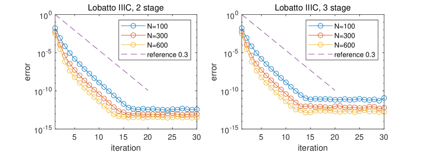
In example (a), the data is sufficiently smooth and compatible to the homogeneous Dirichlet boundary condition. In fact, it is easy to show show that u0Dom((Δ)3+ϵ)superscript𝑢0DomsuperscriptΔ3italic-ϵu^{0}\in\text{Dom}((-\Delta)^{3+\epsilon}) with ϵ(0,1/4)italic-ϵ014\epsilon\in(0,1/4) (see e.g. Lemma [30, Lemma 3.1]). For this case of regular data, Bal showed that the first several parareal iterations converge linearly with the rate O(ΔT)𝑂Δ𝑇O(\Delta T); see cf. [5]. This is fully supported by the numerical results presented in Figure 5.1, where we show the convergence of parareal algorithm for 222- and 333-stage Lobatto IIIC methods with fixed J=10𝐽10J=10 and ΔT=1/100Δ𝑇1100\Delta T=1/100, 1/30013001/300, 1/60016001/600 (and correspondingly Δt=1/1000Δ𝑡11000\Delta t=1/1000, 1/3000130001/3000, 1/6000160001/6000). We observe that the convergence of the first several iterations is faster for smaller coarse step size, but the convergence then deteriorates for the later iterations.

Refer to caption
Figure 5.1: Example 1 (a): smooth data. Convergence of the parareal algorithm for $2$- and $3$-stage Lobatto IIIC methods with fixed mesh ratio $J=10$ and various coarse step sizes $1/N$, $N=100$, $300$, $600$.

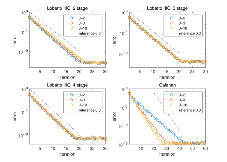
In Figure 5.2, we show the convergence of parareal algorithm for 222-, 333-, 444-stage Lobatto IIIC methods solving parabolic equation with nonsmooth initial data, i.e. Example 1 (b). We fixed the fine step size Δt=1/3000Δ𝑡13000\Delta t=1/3000 and use different step ratios J=2𝐽2J=2, 333 and 101010. The numerical experiments clearly show that the parareal iterations converge linearly with convergence factor near 0.30.30.3 for all J2𝐽2J\geq 2. Meanwhile, we observe that the convergence factor is independent of the ratio between coarse and find step sizes. These phenomenon fully support our theoretical findings in Propositions 4.34.7. Moreover, we test another time integrator, called Calahan scheme [37, eq. (1.9)], defined by

(20) r(s)=1s1+bs36(s1+bs)2,withb=12(1+33)formulae-sequence𝑟𝑠1𝑠1𝑏𝑠36superscript𝑠1𝑏𝑠2with𝑏12133r(-s)=1-\frac{s}{1+bs}-\frac{\sqrt{3}}{6}\Big{(}\frac{s}{1+bs}\Big{)}^{2},\qquad\text{with}~{}~{}b=\frac{1}{2}\Big{(}1+\frac{\sqrt{3}}{3}\Big{)}

and

(21) c1=13,subscript𝑐113\displaystyle c_{1}=\frac{1}{3}, p1(s)=(1/2+3)+(3/2)s(1+bs)2;subscript𝑝1𝑠12332𝑠superscript1𝑏𝑠2\displaystyle p_{1}(-s)=\frac{(1/2+\sqrt{3})+(\sqrt{3}/2)s}{(1+bs)^{2}};
c2=23,subscript𝑐223\displaystyle c_{2}=\frac{2}{3}, p2(s)=(1/23)+(1/23/2)s(1+bs)2.subscript𝑝2𝑠1231232𝑠superscript1𝑏𝑠2\displaystyle p_{2}(-s)=\frac{(1/2-\sqrt{3})+(1/2-\sqrt{3}/2)s}{(1+bs)^{2}}.

The Butcher tableau is given by

(22) 163+231631313163+13163+13231212=:𝒪ιcb\begin{tabular}[]{cc|c}$\frac{1}{6}\sqrt{3}+\frac{2}{3}$&$-\frac{1}{6}\sqrt{3}-\frac{1}{3}$&$\frac{1}{3}$\\[2.0pt] $-\frac{1}{6}\sqrt{3}+\frac{1}{3}$&$\frac{1}{6}\sqrt{3}+\frac{1}{3}$&$\frac{2}{3}$\\[2.0pt] \hline\cr$\frac{1}{2}$&$\frac{1}{2}$&$\;$\\ \end{tabular}\ =:\begin{tabular}[]{c|c}$\text{${\mathcal{O}}\hskip-3.0pt\iota$}$&$c$\\[1.0pt] \hline\cr$b^{\top}$&$\vphantom{\sum^{\sum^{\sum}}}$\\ \end{tabular}

It is easy to see that r(s)𝑟𝑠r(-s) is a decreasing function on (0,)0(0,\infty) and r()=13(1,0)𝑟1310r(-\infty)=1-\sqrt{3}\in(-1,0), so it is A-stable, but not L-stable. Besides, the scheme is accurate of order k=3𝑘3k=3. Therefore, the Calahan scheme satisfies Conditions (P1)–(P3). Numerical results show that the converegnce of the corresponding parareal iterations is much slower than 0.30.30.3 for small J𝐽J. This might be due to the fact that |r()|>0𝑟0|r(-\infty)|>0; see Remark 4.10. However, for large J𝐽J, the numerical results indicate a convergence rate close to 0.30.30.3, as predicted by Theorem 3.7.

Refer to caption
Figure 5.2: Example 1 (b): nonsmooth data. Convergence of the parareal algorithm for $2$-, $3$-, $4$-stage Lobatto IIIC methods and Calahan method with fixed fine step size $\Delta t=1/3000$ and various ratios of coarse step size and fine step size.

Example 2. Semilinear Parabolic Equations

In this part, we shall examine the convergence of parareal algorithm for solving the initial-boundary value problem of the semilinear parabolic equations

(23) {tuxxu=1ϵ2(uu3)=:f(u),for allxΩ,t(0,T],xu(x,t)=0,for allx{0,π},t(0,T],u(x,0)=u0(x),for allxΩ.\left\{\begin{aligned} \partial_{t}u-\partial_{xx}u&=\frac{1}{\epsilon^{2}}(u-u^{3})=:f(u),\quad\text{for all}~{}~{}x\in\Omega,t\in(0,T],\\ \partial_{x}u(x,t)&=0,\qquad\qquad\text{for all}~{}~{}x\in\{0,\pi\},t\in(0,T],\\ u(x,0)&=u^{0}(x),\quad\quad\text{for all}~{}~{}x\in\Omega.\end{aligned}\right.

The model (23), called Allen–Cahn equation, was originally introduced by Allen and Cahn in [2] to describe the motion of anti-phase boundaries in crystalline solids. In the context, u𝑢u represents the concentration of one of the two metallic components of the alloy and the parameter ϵitalic-ϵ\epsilon involved in the nonlinear term represents the width of interface. Recent decades, the Allen–Cahn equation has become one of basic phase-field equations, which has been widely applied to many complicated moving interface problems in materials science and fluid dynamics [3, 8, 36].

In our numerical scheme, the coarse propagator is the semli-implicit backward Euler scheme: for given $u^{n}$, look for $u^{n+1}$ such that for all $\phi\in H^{1}(0,\pi)$

$$(u^{n+1},\phi)+\Delta T(\partial_{x}u^{n+1},\partial_{x}\phi)=(u^{n},\phi)+\Delta T(f(u^{n}),\phi),$$

which is uniquely solvable and first-order accurate, see e.g. [30, Theorem 14.7]. Meanwhile, the fine propagator is an arbitrary fully implicit high-order single step integrator (such as the Lobatto IIIC schemes or the fully implicit Calahan scheme): for given unsuperscript𝑢𝑛u^{n}, look for un+1superscript𝑢𝑛1u^{n+1} such that for all ϕH1(0,π)italic-ϕsuperscript𝐻10𝜋\phi\in H^{1}(0,\pi)

(24) {(uni,ϕ)=(un1,ϕ)+Δtj=1maij((xunj,xϕ)+(f(unj),ϕ))for1iq,(un,ϕ)=(un1,ϕ)+Δti=1mbi((xuni,xϕ)+(f(uni),ϕ)),\left\{\begin{aligned} (u^{ni},\phi)&=(u^{n-1},\phi)+\Delta t\sum_{j=1}^{m}a_{ij}\Big{(}-(\partial_{x}u^{nj},\partial_{x}\phi)+(f(u^{nj}),\phi)\Big{)}~{}~{}\text{for}~{}1\leq i\leq q,\\ (u^{n},\phi)&=(u^{n-1},\phi)+\Delta t\sum_{i=1}^{m}b_{i}\Big{(}-(\partial_{x}u^{ni},\partial_{x}\phi)+(f(u^{ni}),\phi)\Big{)},\end{aligned}\right.

where the nonlinear system is uniquely solvable for sufficiently small step size, and we solve it by use Newton’s algorithm. Note that the fine propagator is fully nonlinear and hence time consuming where the coarse propagator is a linear scheme, so the application of parareal algorithm is able to significantly improve the efficiency.

Refer to caption
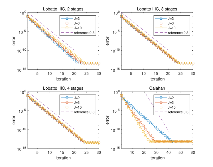
Figure 5.3: Example 2. Convergence of the parareal algorithm for $2$-, $3$-, $4$-stage Lobatto IIIC methods and Calahan method with fine step size $\Delta t=1/600$ and various step ratios $J=2$, $3$, $10$.

In Figure 5.3, we show the convergence of parareal algorithm for 222-, 333-, 444-stage Lobatto IIIC methods and the Calahan method solving the semilinear parabolic equation (23) with ϵ=1italic-ϵ1\epsilon=1 and T=0.1𝑇0.1T=0.1. The fine step size is fixed and we examine the convergence for different step ratios. Similar to the linear problem, for Lobatto IIIC methods, the numerical experiments clearly show that the parareal iterations converge linearly with convergence factor near 0.30.30.3 for all J2𝐽2J\geq 2, while for the Calahan method the parareal iterations converge slowly for a small J𝐽J. The convergence analysis for the nonlinear problem warrants further investigation in our future studies.

6 Conclusion

In this paper, we revisit the popular parareal algorithm for solving the linear parabolic equations, where the coarse propagator is fixed to the backward Euler method and the fine propagator could be an arbitrarily high-order single step integrator. If the stability function of the fine propagator satisfies |r()|<1𝑟1|r(-\infty)|<1, we show that there must exist some critical threshold J>0subscript𝐽0J_{*}>0 such that the parareal solver converges as fast as Parareal-Euler with a convergence rate near 0.30.30.3, provided that the ratio between the coarse time step and fine time step, named as J𝐽J, satisfies JJ𝐽subscript𝐽J\geq J_{*}. The convergence is robust even if the problem data is nonsmooth. Moreover, we examine some popular high-order single step methods, e.g., two-, three- and four-stage Lobatto IIIC methods, and verify a convergence factor 0.310.310.31 with the threshold J=2subscript𝐽2J_{*}=2. The argument in the paper could be easily extended to the convection-diffusion equations. Numerical experiments fully support our theoretical findings.

Some interesting questions are still open:

  • First of all, the argument in the paper, relies on the spectrum decomposition, which only works for the linear parabolic problem (with time-independent operator $A$). How to extend the argument to the case that $A$ is time-dependent and the nonlinear problem is still unclear. One possible approach is to combine the current analysis and the perturbation argument, as people did for the classical error analysis. Besides, in order to keep some important physical properties, like the maximum principle in the parabolic system, or the energy stable in the gradient flow system, many strategies are proposed in the development of numerical schemes, such as stabilization method [27, 10], IEQ/SAV method [28, 35], postprocessing method [18, 31]. The parareal algorithm for those novel methods awaits theoretical studies.

  • Moreover, in the current paper, we only consider the algorithm where the elliptic operator $A$ for the coarse and fine propagators keeps the same, which means we use the same spatial discretization. It is also interesting to analyze the parareal algorithm in the case that the spatial mesh sizes for coarse and fine propagators are different, i.e. $h_{\text{coarse}}\gg h_{\text{fine}}$. This is closely related to the space-time two grid method, whose convergence rate (robust with respect to the problem data) still awaits theoretical justification.

  • Finally, we are interested in the parareal algorithm where the coarse or the fine propagators are stable linear multistep integrators. Both the development and the analysis of such algorithms are completely open, and the argument in current paper is not directly applicable. See some preliminary discussion about BDF2 scheme in [1].

References

  • [1] K. Ait-Ameur, Y. Maday, and M. Tajchman, Multi-step variant of the parareal algorithm, in Domain decomposition methods in science and engineering XXV, vol. 138 of Lect. Notes Comput. Sci. Eng., Springer, Cham, [2020] ©2020, pp. 393–400.
  • [2] S. M. Allen and J. W. Cahn, A microscopic theory for anti-phase boundary motion and its application to anti-phase domain coarsening, Acta Metall, 27 (1979), pp. 1085–1095.
  • [3] D. M. Anderson, G. B. McFadden, and A. A. Wheeler, Diffuse-interface methods in fluid mechanics, Annual review of fluid mechanics, 30 (1998), pp. 139–165.
  • [4] L. Baffico, S. Bernard, Y. Maday, G. Turinici, and G. Zérah, Parallel-in-time molecular-dynamics simulations, Phys. Rev. E, 66 (2002), p. 057701.
  • [5] G. Bal, On the convergence and the stability of the parareal algorithm to solve partial differential equations, in Domain decomposition methods in science and engineering, vol. 40 of Lect. Notes Comput. Sci. Eng., Springer, Berlin, 2005, pp. 425–432.
  • [6] P. Brenner, M. Crouzeix, and V. Thomée, Single-step methods for inhomogeneous linear differential equations in Banach space, RAIRO Anal. Numér., 16 (1982), pp. 5–26.
  • [7] J. C. Butcher, On the implementation of implicit Runge-Kutta methods, Nordisk Tidskr. Informationsbehandling (BIT), 16 (1976), pp. 237–240.
  • [8] L.-Q. Chen, Phase-field models for microstructure evolution, Annual review of materials research, 32 (2002), pp. 113–140.
  • [9] J. Cortial and C. Farhat, A time-parallel implicit method for accelerating the solution of non-linear structural dynamics problems, Internat. J. Numer. Methods Engrg., 77 (2009), pp. 451–470.
  • [10] Q. Du, L. Ju, X. Li, and Z. Qiao, Maximum bound principles for a class of semilinear parabolic equations and exponential time-differencing schemes, SIAM Rev., 63 (2021), pp. 317–359.
  • [11] B. L. Ehle, On Padé approximations to the exponential function and A-stable methods for the numerical solution of initial value problems, ProQuest LLC, Ann Arbor, MI, 1969. Thesis (Ph.D.)–University of Waterloo (Canada).
  • [12] C. Farhat and M. Chandesris, Time-decomposed parallel time-integrators: theory and feasibility studies for fluid, structure, and fluid-structure applications, Internat. J. Numer. Methods Engrg., 58 (2003), pp. 1397–1434.
  • [13] M. J. Gander, 50 years of time parallel time integration, in Multiple shooting and time domain decomposition methods, vol. 9 of Contrib. Math. Comput. Sci., Springer, Cham, 2015, pp. 69–113.
  • [14] M. J. Gander and S. Vandewalle, Analysis of the parareal time-parallel time-integration method, SIAM J. Sci. Comput., 29 (2007), pp. 556–578.
  • [15] E. Hairer and G. Wanner, Solving ordinary differential equations. II, vol. 14 of Springer Series in Computational Mathematics, Springer-Verlag, Berlin, 2010. Stiff and differential-algebraic problems, Second revised edition, paperback.
  • [16] K. R. Jackson and S. P. Nø rsett, The potential for parallelism in Runge-Kutta methods. I. RK formulas in standard form, SIAM J. Numer. Anal., 32 (1995), pp. 49–82.
  • [17] O. A. Karakashian and W. Rust, On the parallel implementation of implicit Runge-Kutta methods, SIAM J. Sci. Statist. Comput., 9 (1988), pp. 1085–1090.
  • [18] B. Li, J. Yang, and Z. Zhou, Arbitrarily high-order exponential cut-off methods for preserving maximum principle of parabolic equations, SIAM J. Sci. Comput., 42 (2020), pp. A3957–A3978.
  • [19] X. Li, T. Tang, and C. Xu, Parallel in time algorithm with spectral-subdomain enhancement for Volterra integral equations, SIAM J. Numer. Anal., 51 (2013), pp. 1735–1756.
  • [20] J.-L. Lions, Y. Maday, and G. Turinici, Résolution d’EDP par un schéma en temps “pararéel”, C. R. Acad. Sci. Paris Sér. I Math., 332 (2001), pp. 661–668.
  • [21] Y. Maday, J. Salomon, and G. Turinici, Monotonic parareal control for quantum systems, SIAM J. Numer. Anal., 45 (2007), pp. 2468–2482.
  • [22] T. P. Mathew, M. Sarkis, and C. E. Schaerer, Analysis of block parareal preconditioners for parabolic optimal control problems, SIAM J. Sci. Comput., 32 (2010), pp. 1180–1200.
  • [23] J. Nievergelt, Parallel methods for integrating ordinary differential equations, Comm. ACM, 7 (1964), pp. 731–733.
  • [24] B. W. Ong and J. B. Schroder, Applications of time parallelization, Comput. Vis. Sci., 23 (2020), pp. Paper No. 11, 15.
  • [25] J. Reynolds-Barredo, D. Newman, R. Sanchez, D. Samaddar, L. Berry, and W. Elwasif, Mechanisms for the convergence of time-parallelized, parareal turbulent plasma simulations, Journal of Computational Physics, 231 (2012), pp. 7851–7867.
  • [26] J. M. Reynolds-Barredo, D. E. Newman, and R. Sanchez, An analytic model for the convergence of turbulent simulations time-parallelized via the parareal algorithm, J. Comput. Phys., 255 (2013), pp. 293–315.
  • [27] J. Shen, T. Tang, and J. Yang, On the maximum principle preserving schemes for the generalized Allen-Cahn equation, Commun. Math. Sci., 14 (2016), pp. 1517–1534.
  • [28] J. Shen, J. Xu, and J. Yang, A new class of efficient and robust energy stable schemes for gradient flows, SIAM Rev., 61 (2019), pp. 474–506.
  • [29] G. A. Staff and E. M. Rø nquist, Stability of the parareal algorithm, in Domain decomposition methods in science and engineering, vol. 40 of Lect. Notes Comput. Sci. Eng., Springer, Berlin, 2005, pp. 449–456.
  • [30] V. Thomée, Galerkin Finite Element Methods for Parabolic Problems, Springer-Verlag, Berlin, second ed., 2006.
  • [31] J. J. W. van der Vegt, Y. Xia, and Y. Xu, Positivity preserving limiters for time-implicit higher order accurate discontinuous Galerkin discretizations, SIAM J. Sci. Comput., 41 (2019), pp. A2037–A2063.
  • [32] S.-L. Wu, Convergence analysis of some second-order parareal algorithms, IMA J. Numer. Anal., 35 (2015), pp. 1315–1341.
  • [33] S.-L. Wu and T. Zhou, Convergence analysis for three parareal solvers, SIAM J. Sci. Comput., 37 (2015), pp. A970–A992.
  • [34]  , Fast parareal iterations for fractional diffusion equations, J. Comput. Phys., 329 (2017), pp. 210–226.
  • [35] X. Yang, J. Zhao, and Q. Wang, Numerical approximations for the molecular beam epitaxial growth model based on the invariant energy quadratization method, J. Comput. Phys., 333 (2017), pp. 104–127.
  • [36] P. Yue, J. J. Feng, C. Liu, and J. Shen, A diffuse-interface method for simulating two-phase flows of complex fluids, Journal of Fluid Mechanics, 515 (2004), p. 293.
  • [37] M. Zlámal, Finite element methods for parabolic equations, Math. Comp., 28 (1974), pp. 393–404.