Two-timescale Mechanism-and-Data-Driven Control for Aggressive Driving of Autonomous Cars

Abstract

The control for aggressive driving of autonomous cars is challenging due to the presence of significant tyre slip. Data-driven and mechanism-based methods for the modeling and control of autonomous cars under aggressive driving conditions are limited in data efficiency and adaptability respectively. This paper is an attempt toward the fusion of the two classes of methods. By means of a modular design that is consisted of mechanism-based and data-driven components, and aware of the two-timescale phenomenon in the car model, our approach effectively improves over previous methods in terms of data efficiency, ability of transfer and final performance. The hybrid mechanism-and-data-driven approach is verified on TORCS (The Open Racing Car Simulator). Experiment results demonstrate the benefit of our approach over purely mechanism-based and purely data-driven methods.

I Introduction

In recent years, autonomous cars have demonstrated vast potential in terms of increasing road efficiency, reducing accidents and alleviating environmental impact [1]. The development of high (L4) and full (L5) driving automation has been put on the agenda worldwide, and improving the applicability of autonomous driving in complicated road conditions has drawn significant research attention [2, 3, 4].

This paper considers the control of autonomous cars under aggressive driving conditions. Subject to the difficulty of control under high speed and with the presence of significant tyre slip, existing practical driving automation schemes usually adopt conservative policies, and the driving efficiency has room for improvement. Therefore, aggressive autonomous driving scenes like high-speed off-road driving [5] and autonomous overtaking [6] have been studied in recent years. Research into how to make the car execute aggressive driving behavior while ensuring safety would help us explore the boundary of autonomous driving, and provide technical insights toward high and full driving automation.

We adopt a modular approach to the modeling and control of autonomous cars. In particular, we split the car model into modules with fast and slow timescales, and propose a controller with mechanism-based and data-driven modules. The simplified mechanism for driving an autonomous car is i) the controller changes the steering angle and exerts torques to the wheels; ii) the tyres respond to the steering angle and the torques, yielding friction forces through tyre-road interaction; iii) the friction forces cause the pose of the car body to change. We observe that friction forces respond to the control inputs much faster than the pose of the car, because the inertia of a wheel is much smaller than that of the car body. In other words, the wheels correspond to the fast timescale, while the car body corresponds to the slow timescale, and this observation enables us to design an efficient two-timescale control scheme. Furthermore, we notice that the car body can be idealized as a rigid body, which can be readily modeled and controlled from first principles, while the tyre-road interaction characteristic is a highly nonlinear function between the slip ratio and the friction force that can only be described by an empirical formula called Pacejka Magic Formula [7], which involves parameters that are difficult to measure, necessitating data-driven modeling. Therefore, we include a mechanism-based module for driving the rigid body and a data-driven module for dealing with the tyre-road interaction in our control policy. This strategy demonstrates higher data efficiency than the purely data-driven scheme and better adaptability than the purely mechanism-based scheme.

Existing research papers have studied integrating mechanism-based and data-driven control methods in autonomous driving tasks from different aspects. Rosolia et al. [8] addresses the racing task by applying Model Predictive Control (MPC) to track a reference trajectory that is iteratively learned on a lap-to-lap basis. However, it assumes a relatively accurate low-level dynamics model of the car is obtained a priori through system identification, and suffers from limited generalization across different tyre-road interaction characteristics, which restricts its applicability in general high-performance driving tasks. Hewing et al. [9] models the car dynamics as the sum of the nominal dynamics and a Gaussian Process (GP), which leverages the power of both mechanism and data, but it makes no distinction between mechanism-based and data-driven modules. By contrast, we adopt a modular design that marks a clear boundary between mechanism-based and data-driven components, and explicitly considers the two-timescale issue mentioned above. This modular design improves the explainability of control policy, and is suitable for the deployment over various aggressive driving scenarios.

To summarize, in this paper we propose a two-timescale control scheme for aggressive autonomous driving that combines mechanism-based and data-driven methods. We verify our method on both a simplified car model with tyre slip and TORCS racing simulator [10]. Simulation results show that our proposed method can achieve significantly higher data efficiency than the purely data-driven method, and is more adaptive to various driving conditions than the purely mechanism-based method.

II Problem Formulation

We use the bicycle model with tyre slip and load transfer [5] for simulation and control, illustrated in Fig. 1.

Figure 1: Illustration of car model

The state and input vectors are

$$\mathbf{X}=\left[x,y,\psi,\dot{x},\dot{y},\dot{\psi},\omega_{f},\omega_{r}\right]^{\top},\mathbf{U}=\left[\delta,T_{f},T_{r}\right]^{\top},$$ (1)

where $x,y$ are the coordinate of the car in a two-dimensional plane, $\psi$ is the heading angle of the car, $\dot{x},\dot{y},\dot{\psi}$ are the time derivatives of $x,y,\psi$; $\omega_{f},\omega_{r}$ are the rotational speed of the front and rear wheels respectively, $\delta$ is the steering angle, and $T_{f},T_{r}$ are the torques exerted on the front and rear wheels respectively. The dynamic equations are

$$m\ddot{x} =f_{fx}^{w}\cos(\psi+\delta)-f_{fy}^{w}\sin(\psi+\delta)+f_{rx}^{b}\cos\psi-f_{ry}^{b}\sin\psi,$$ (2)

$$m\ddot{y} =f_{fx}^{w}\sin(\psi+\delta)+f_{fy}^{w}\cos(\psi+\delta)+f_{rx}^{b}\sin\psi+f_{ry}^{b}\cos\psi,$$ (3)

$$I_{z}\ddot{\psi} =\left(f_{fy}^{w}\cos\delta+f_{fx}^{w}\sin\delta\right)l_{f}-f_{ry}^{b}l_{r},$$ (4)

$$I_{f}\dot{\omega}_{f} =T_{f}-f_{fx}^{w}r_{f},I_{r}\dot{\omega}_{r}=T_{r}-f_{rx}^{b}r_{r},$$ (5)

where $m$ is the mass of the car, $I_{z}$ is the moment of inertia of the car body w.r.t. the $z$ axis, $I_{f},I_{r}$ are the moments of inertia of the wheels, $r_{f},r_{r}$ are the radii of the wheels, $l_{f},l_{r}$ are the distances of the wheels to the center of mass of the car, and $f_{fx}^{w},f_{fy}^{w},f_{rx}^{b},f_{ry}^{b}$ are the friction forces. The subscripts ‘f’, ‘r’ refer to “front” and “rear” respectively, and the superscripts ‘w’ and ‘b’ refer to “front wheel frame” and “body frame” respectively. It shall be noticed that the use of these two coordinate systems facilitates the decomposition of body and wheel dynamics. The forces are determined by

$$f_{fx}^{w}=\mu_{fx}f_{fz},f_{fy}^{w}=\mu_{fy}f_{fz},f_{rx}^{b}=\mu_{rx}f_{rz},f_{ry}^{b}=\mu_{ry}f_{rz},$$

where $\mu_{fx},\mu_{fy},\mu_{rx},\mu_{ry}$ are the friction coefficients, and $f_{fz},f_{rz}$ are the normal forces. The friction coefficients are described by Pacejka Magic Formula [7]:

$$\mu_{ij}=-\frac{s_{ij}}{s_{i}}D\sin\left(C\arctan(Bs_{i})\right)\;\left(i\in\{f,r\},\;j\in\{x,y\}\right),$$ (6)

where $B,C,D$ are parameters that vary with the tyre-road interaction properties, and $s_{i},s_{ij}$ are slip ratios that can be computed from relative speeds between the wheels and the road:

$$s_{i}=\sqrt{s_{ix}^{2}+s_{iy}^{2}},\quad\left(i\in\{f,r\}\right),$$ (7)

$$s_{fx}=\frac{v_{fx}^{w}-\omega_{f}r_{f}}{\omega_{f}r_{f}},s_{fy}=\frac{v_{fy}^{w}}{\omega_{f}r_{f}},$$ (8)

$$s_{rx}=\frac{v_{rx}^{b}-\omega_{r}r_{r}}{\omega_{r}r_{r}},s_{ry}=\frac{v_{ry}^{b}}{\omega_{r}r_{r}},$$ (9)

$$v=\sqrt{\dot{x}^{2}+\dot{y}^{2}},\beta=\arctan\frac{\dot{y}}{\dot{x}}-\psi,$$ (10)

$$v_{fx}^{w}=v\cos(\beta-\delta)+\dot{\psi}l_{f}\sin\delta,v_{rx}^{b}=v\cos\beta,$$ (11)

$$v_{fy}^{w}=v\sin(\beta-\delta)+\dot{\psi}l_{f}\cos\delta,v_{ry}^{b}=v\sin\beta-\dot{\psi}l_{r}.$$ (12)

Finally, the normal forces $f_{fz},f_{rz}$ can be determined as:

$$f_{fz}=\frac{l_{r}-\mu_{rx}h}{l_{f}+l_{r}+\left(\mu_{fx}\cos\delta-\mu_{fy}\sin\delta-\mu_{rx}\right)h}mg,$$

$$f_{rz}=\frac{l_{f}+\left(\mu_{fx}\cos\delta-\mu_{fy}\sin\delta\right)h}{l_{f}+l_{r}+\left(\mu_{fx}\cos\delta-\mu_{fy}\sin\delta-\mu_{rx}\right)h}mg.$$

The goal of the controller is to drive the car to optimize some certain performance metrics subject to safety constraints, without prior knowledge of the tyre-road interaction parameters $B,C,D$. We assume all the state variables can be directly measured. Mathematically, the controller should approximately solve the optimal control problem

$$\begin{aligned} &\min_{\mathbf{X}_{0:T-1},\mathbf{U}_{0:T-1}}J\left(\mathbf{X}_{0:T-1},\mathbf{U}_{0:T-1}\right),\\ &\text{s.t. }\mathbf{X}_{t+1}=f\left(\mathbf{X}_{t},\mathbf{U}_{t}\right),\mathbf{X}_{t}\in\mathcal{X},\mathbf{U}_{t}\in\mathcal{U},\mathbf{X}_{0}=\mathbf{X}_{\text{init}},\end{aligned}$$ (13)

where $\mathbf{X}_{t},\mathbf{U}_{t}$ are state and input vectors respectively, as defined in (1), $T$ is the control horizon, $J$ is the performance metrics, $f$ is the dynamics function, $\mathcal{X},\mathcal{U}$ are the constraint sets on the state and input respectively, and $\mathbf{X}_{\text{init}}$ is the initial state. In particular, we consider the following tasks in this paper:

• Low-level task - path tracking: track a manually specified path with high speed and large curvature in an infinite plane. In this task, $J$ is the tracking error, $f$ is the discretized system of the dynamics described in (2)-(5), $\mathcal{U}$ is the maneuver limit of the car, and there is no additional constraint on the state.

• High-level task - racing: race on TORCS platform with tracks in different shapes. In this task, $J$ is the lap time, $f$ is a high-fidelity simulation model more complicated than the one described in this section, $\mathcal{U}$ is the maneuver limit of the car, and $\mathcal{X}$ represent the road boundaries.

III Controller Design

In this section, we first illustrate the two-timescale phenomenon in car model using an example, which reveals the rationale behind our modular design. Afterwards, we describe the mechanism-based and data-driven components of our controller. A schematic diagram of the closed-loop system of the car driven by our controller is shown in Fig. 2.

Figure 2: Schematic diagram of closed-loop system

III-A Two-timescale phenomenon in car model

In theory, it is possible to find an approximate solution to the optimal control problem (13) using Model Predictive Control (MPC), which can be solved numerically using a nonlinear solver such as Ipopt [11]. However, we next illustrate with an example that this is impractical.

In the following example, we instantiate the simulation model in Section II with the geometric and mechanical parameters of a Mercedes CLS 63 AMG car and the tyre-road interaction parameters of a typical tarmac road ($B=10,C=1.9,D=1$). We choose the frequency of the controller to be $10\mathrm{Hz}$ and discretize the dynamics model (2)-(5) with fourth-order Runge-Kutta method. We apply MPC to track the reference trajectory shown in Fig. 3(a). It can be observed from Fig. 3 that the controller cannot achieve reasonable tracking performance even though the computation is already slower than real time.

(a) Comparison of reference trajectory and actual trajectory

(b) Computation time

Figure 3: Result of directly applying MPC

To analyze why the direct application of MPC fails, we inspect the Jacobian matrix $A(t)=\left.\frac{\partial\left[\dot{\psi},\ddot{x},\ddot{y},\ddot{\psi},\dot{\omega}_{f},\dot{\omega}_{r}\right]^{\top}}{\partial\left[{\psi},\dot{x},\dot{y},\dot{\psi},{\omega}_{f},{\omega}_{r}\right]^{\top}}\right|_{\mathbf{X}=\mathbf{X}(t),\mathbf{U}=\mathbf{U}(t)}$ at a particular time step $t$ along the reference trajectory. We have

$$A(t)\approx\left[\begin{array}[]{cccccc}0&0&0&1&0&0\\ 0&-200&0&0&32.0&33.6\\ 1.05&0&-194&7.91&0&0\\ 0&0&11.3&-567&0&0\\ 0&1.4\mathrm{e}4&0&0&-4.6\mathrm{e}3&-4.29\\ 0&1.8\mathrm{e}4&0&0&-208&-5.7\mathrm{e}3\end{array}\right],$$

of which the eigenvalue with largest absolute value is $\bar{\lambda}\approx-1.16\times 10^{3}$, and the eigenvalue of the smallest absolute value is $\underline{\lambda}\approx 2.16\times 10^{-5}$. We have $|\bar{\lambda}|/|\underline{\lambda}|\approx 5.37\times 10^{7}$, which indicates $A(t)$ is a highly ill-conditioned matrix. It is known from the theory of numerical solutions for ordinary differential equations [12] that the differential equation $\dot{\mathbf{X}}=\dot{\mathbf{X}}\left(\mathbf{X},\mathbf{U}\right)$ has a high stiffness ratio, and therefore, explicit solvers like Euler and Runge-Kutta are numerically unstable for this differential equation unless the step size is taken extremely small. Correspondingly, the discretization $\mathbf{X}_{t+1}=f\left(\mathbf{X}_{t},\mathbf{U}_{t}\right)$ in the MPC formulation (13) is very inaccurate under normal step sizes, posing challenge to the implementation of the controller.

From a physical point of view, the inertia of the wheels are significantly smaller than that of the car body, and therefore the wheels respond to changes much faster than the car body. In the matrix $A(t)$ demonstrated above, the elements with largest magnitudes are $\frac{\partial\dot{\omega}_{f}}{\partial\dot{x}},\frac{\partial\dot{\omega}_{r}}{\partial\dot{x}},\frac{\partial\dot{\omega}_{f}}{\partial\omega_{f}},\frac{\partial\dot{\omega}_{r}}{\partial\omega_{r}}$, which means the change of wheel rotational speeds is very sensitive to the current rotational speed and the longitudinal speed of the car. By contrary, the pose of the car body is not very sensitive to the instantaneous states and inputs, and the inputs need to be accumulated over time in order to drive the car to the desired pose. The above observation can be summarized as a two-timescale phenomenon, which we explicitly consider in our controller design. In particular, at the slow timescale, we design a controller to make the car body track the reference trajectory assuming the friction forces $f_{fx},f_{fy},f_{rx},f_{ry}$ can be directly controlled, while at the fast timescale, we solve for the actual control inputs that yield the desired forces assuming the motion of the car body is constant. This modular design is described in detail in the following subsections.

III-B Mechanism-based controller

At the slow timescale, we focus our attention on the car body, and use MPC to solve for the desired friction forces based on rigid-body mechanics principles. The state vector for this MPC is the pose of the car body along with its derivative. Next we determine the input vector for the MPC. Since the forces should be independent of the steering angle of the front wheel $\delta$ at the slow timescale, we cast $f_{fx}^{w},f_{fy}^{w}$ into the body frame through the identity

$$\left[\begin{array}[]{c}f_{fx}^{b}\\ f_{fy}^{b}\end{array}\right]=\left[\begin{array}[]{cc}\cos\delta&-\sin\delta\\ \sin\delta&\cos\delta\end{array}\right]\left[\begin{array}[]{l}f_{fx}^{w}\\ f_{fy}^{w}\end{array}\right]$$

as illustrated in Fig. 1. To summarize, the state and input vectors for the MPC are

$$\mathbf{q}=\left[x,y,\psi,\dot{x},\dot{y},\dot{\psi}\right]^{\top},\mathbf{f}=\left[f_{fx}^{b},f_{rx}^{b},f_{fy}^{b},f_{ry}^{b}\right]^{\top}.$$

The controller solves the tracking problem

$$\begin{aligned} &\min_{\mathbf{q}_{0:T-1},\mathbf{f}_{0:T-1}}\sum_{t=0}^{T-1}\left(\mathbf{q}_{t}-\mathbf{q}^{\text{ref}}_{t}\right)^{\top}\mathbf{Q}\left(\mathbf{q}_{t}-\mathbf{q}^{\text{ref}}_{t}\right)+\mathbf{f}_{t}^{\top}\mathbf{R}\mathbf{f}_{t},\\ &\text{s.t. }\mathbf{q}_{t+1}=f\left(\mathbf{q}_{t},\mathbf{f}_{t}\right),\underline{\mathbf{f}}\leq\mathbf{f}_{t}\leq\bar{\mathbf{f}},\mathbf{q}_{0}=\mathbf{q}_{\text{current}},\end{aligned}$$ (14)

at each step and takes $\mathbf{f}_{0}$ for further processing as is clarified later in this subsection. In (14), $T$ is the horizon for the MPC, $\mathbf{Q},\mathbf{R}$ are fixed positive-definite weight matrices, $f$ is the discretized system of the rigid-body equations (2)-(4), and $\underline{\mathbf{f}},\bar{\mathbf{f}}$ are approximate lower and upper bounds for the corresponding forces that are specified by design choices. We assume that reference trajectory $\left\{\mathbf{q}^{\text{ref}}_{t}\right\}$ is available to MPC, either manually specified or provided by a task-specific planner module.

At the fast timescale, we focus our attention on the wheels, in order to translate the desired friction forces $\mathbf{f}_{0}$ obtained from the MPC at the slow timescale into actual control inputs $\mathbf{U}$. In particular, we assume $\mathbf{q}$ which describes the pose and motion of the car body is constant, in which situation we choose the steering angle and torques to make the actual friction forces as close to $\mathbf{f}_{0}$ as possible. We will proceed in two steps. Firstly, we convert the desired friction forces into the steering angle $\delta$ and the slip ratios $s_{fx},s_{fy},s_{rx},s_{ry}$. Secondly, we determine the torques that would lead to the desired slip ratios.

We exploit the coupling between lateral and longitudinal slip to determine the desired slip ratios. From (6) and (9) we have

$$\frac{s_{rx}}{s_{ry}}=\frac{\mu_{rx}}{\mu_{ry}}=\frac{f_{rx}^{b}}{f_{ry}^{b}},\frac{s_{rx}+1}{s_{ry}}=\frac{v_{rx}^{b}}{v_{ry}^{b}},$$

and by taking the difference of the above to equalities, we have

$$s_{ry}=\left(\frac{v_{rx}^{b}}{v_{ry}^{b}}-\frac{f_{rx}^{b}}{f_{ry}^{b}}\right)^{-1},s_{rx}=\frac{f_{rx}^{b}}{f_{ry}^{b}}\left(\frac{v_{rx}^{b}}{v_{ry}^{b}}-\frac{f_{rx}^{b}}{f_{ry}^{b}}\right)^{-1}.$$

According to the “constant motion” assumption for the fast timescale, we can substitute the measured velocity components $v_{rx}^{b},v_{ry}^{b}$ into the above equation to obtain the desired $s_{rx},s_{ry}$. Similarly, for the front wheel we have

$$\frac{s_{fx}}{s_{fy}}=\frac{\mu_{fx}}{\mu_{fy}}=\frac{f_{fx}^{w}}{f_{fy}^{w}}=\frac{\cos\delta f_{fx}^{b}+\sin\delta f_{fy}^{b}}{-\sin\delta f_{fx}^{b}+\cos\delta f_{fy}^{b}},$$

$$\frac{s_{fx}+1}{s_{fy}}=\frac{v_{fx}^{w}}{v_{fy}^{w}}=\frac{v\cos(\beta-\delta)+\dot{\psi}l_{f}\sin\delta}{v\cos\beta},$$

from which we can represent $s_{fx},s_{fy}$ as functions of $\delta$. To determine the steering angle $\delta$, we impose the constraint that the total slip on the front wheel $s_{f}(\delta)=\sqrt{s_{fx}(\delta)^{2}+s_{fy}(\delta)^{2}}$ should yield the total desired friction force on the front wheel, i.e., $\delta$ should satisfy the equation

$$D\sin\left(C\arctan\left(Bs_{f}(\delta)\right)\right)=\frac{\sqrt{\left(f_{fx}^{b}\right)^{2}+\left(f_{fy}^{b}\right)^{2}}}{f_{fz}}.$$ (15)

By substituting the unknown tyre-road interaction parameters $B,C,D$ by their estimated values provided by the data-driven module described in the next subsection, and $f_{fz}$ by its measured value, we can solve the nonlinear equation (15) numerically to obtain $\delta$, and hence $s_{fx},s_{fy}$.

To determine the torques, we first compute how much change in wheel rotational speeds $\omega_{f},\omega_{r}$ we need in order to achieve the desired slip ratios, and then apply linear approximation to the wheel dynamics (5) to obtain $T_{f},T_{r}$. To clarify, let us take the front wheel as an example, and linear approximation of (5) results in

$${\omega}_{f}(t)\approx\omega_{f}(0)+\frac{t}{I_{f}}\left(T_{f}-f_{fx}^{w}r_{f}\right).$$ (16)

Let the control interval be $\Delta t$, then under the above linear approximation, the average $\omega_{f}$ over an interval is $\omega_{f}(\Delta t/2)$. We command the longitudinal slip produced by the average $\omega_{f}$ to equal the desired longitudinal slip, i.e.,

$$\frac{v_{fx}^{w}}{\omega_{f}(\Delta t/2)r_{f}}-1=s_{fx}.$$ (17)

Combining (16) and (17), we obtain the formula for determining the torque on the front wheel:

$$T_{f}=f_{fx}^{w}r_{f}+\frac{2I_{f}}{\Delta t}\left(\frac{v_{fx}^{w}}{r_{f}(s_{fx}+1)}-\omega_{f}(0)\right),$$ (18)

where $\omega_{f}(0)$ refers to the current measured value of $\omega_{f}$. Completely similarly, for the rear wheel we can obtain

$$T_{r}=f_{rx}^{b}r_{r}+\frac{2I_{r}}{\Delta t}\left(\frac{v_{rx}^{b}}{r_{r}(s_{rx}+1)}-\omega_{r}(0)\right).$$ (19)

So far, we have formulas for all the three input variables $\delta,T_{f},T_{r}$ as specified in (15), (18), (19), which concludes the mechanism-based part of the controller design.

III-C Data-driven parameter estimator

The controller relies on the tyre-road interaction parameters $\Theta=(B,C,D)$ in order to obtain precise control inputs as shown in (15), but those parameters are not known a priori. Therefore, we adopt a data-driven approach to estimate the parameters.

Given a state-input pair $(\mathbf{X},\mathbf{U})$, and the current estimate of parameters ${{\Theta}}$, we can predict $\hat{\mathbf{Y}}\left(\mathbf{X},\mathbf{U};{{\Theta}}\right)=\left[\hat{\ddot{x}},\hat{\ddot{y}},\hat{\ddot{\psi}},\hat{\dot{\omega}}_{f},\hat{\dot{\omega}}_{r}\right]^{\top}$ according to (2)-(5). Meanwhile, by applying the input $\mathbf{U}$ to the car at state $\mathbf{X}$, we can obtain the actual $\mathbf{Y}=\left[\ddot{x},\ddot{y},\ddot{\psi},\dot{\omega}_{f},\dot{\omega}_{r}\right]^{\top}$. The data-driven module learns the parameters by collecting the trajectory data while running the controller and minimizing the error between the prediction and the actual value. Formally, let the collected dataset be $\boldsymbol{D}=\left\{\left(\mathbf{X}^{(i)},\mathbf{U}^{(i)}\right),\mathbf{Y}^{(i)}\right\}_{i=1}^{n}$, then the parameter update rule can be specified as

$$\underset{\Theta}{\operatorname{min}}\;\mathcal{L}(\Theta;\mathcal{D}):=\sum_{i=1}^{n}\ell\left(\hat{\mathbf{Y}}\left(\mathbf{X}^{(i)},\mathbf{U}^{(i)};{{\Theta}}\right),\mathbf{Y}^{(i)}\right)+\mathcal{R}(\Theta),$$

where $\ell\left(\hat{\mathbf{Y}},\mathbf{Y}\right)$ is a loss function, for which we use Huber loss [13] which is robust to modeling and measurement errors, and $\mathcal{R}$ is a regularization term to enforce sensibility of the parameters, for which we use logarithm barriers. Once a new batch of data is available, the parameter update can be performed by stepping in a nonlinear optimization algorithm, e.g. L-BFGS [14].

It shall be pointed out that $\Theta$ can also include parameters that describe other unmodelled effects, such as aerodynamics and suspension, and therefore the data-driven module can complement the mechanism-based module by making up for the simplicity of the model.

IV Simulation

IV-A Tracking task

In this task, the goal is to drive a simulated car with the model described in Section II to track a manually specified reference trajectory. We use the geometric and mechanical parameters of a Mercedes CLS 63 AMG car and the tyre-road interaction parameters of a typical tarmac road ($B=10,C=1.9,D=1$). We choose the control interval to be $\Delta t=0.1\mathrm{s}$. We use this task to benchmark aggressive driving because it requires the car to turn two right angles with radii of about $10\mathrm{m}$ at the speed of about $90\mathrm{km/h}$, and such aggressive cornering can only be achieved with precise control of the slip.

Figure 4: Iterative improvement of tracking performance of our proposed controller

The qualitative tracking performance of our proposed controller and its iterative improvement over trials is shown in Fig. 4. The gray dashed lines stand for the virtual lanes, the thick black line in the middle of the lane stands for the reference trajectory, and the blue lines, from light to dark, stand for the actual performance of different trials of our controller, from early to late. The numbers to the right of the color bar stand for the indices of corresponding trials. We can observe that the tracking performance improves steadily as the controller gets more trials, which proves the effectiveness of our data-driven strategy. We can also observe that the actual trajectory almost coincides with the reference trajectory after about 20 trials, which proves the correctness of our two-timescale mechanism-based controller design when the parameter estimates are accurate.

Next we compare quantitative performance of our proposed method with purely mechanism-based or purely data-driven method, in terms of data efficiency and ability of transfer. We use our proposed mechanism-based controller with access to the true initial tyre-road interaction parameters $B,C,D$ as the mechanism-based baseline, and use a state-of-the-art deep reinforcement learning algorithm, SAC [15], as the data-driven baseline. In the experiment, we first allow each method 1M training samples in the process of repetitively attempting to complete the tracking task, after which we change some experiment conditions (marked by “Transfer” in Fig. 5), and allow each method another 1M training samples for adapting to the changes. The results of this experiment are presented in Fig. 5. For the ease of observation, both the horizontal and vertical axes in Fig. 5 are in logarithm scale.

(a) Reference trajectory changes

(b) Tyre-road interaction property changes

Figure 5: Comparison of data efficiency and ability of transfer

We can observe from Fig. 5 that the tracking Mean-Square Error (MSE) converges to about $0.1\mathrm{m}^{2}$ with significantly less training samples than the data-driven method, which demonstrates the benefit of our method in terms of data efficiency. In Fig. 5(a), we test the ability of transfer by flipping the reference trajectory upside-down. Both the mechanism-based method and our proposed method are unaffected by this change, because they do not depend on a particular reference trajectory. By contrast, the MSE of the data-driven method become very large after this change, which can be explained by the fact that data-driven methods may overfit to a particular task unless they are exposed to data from sufficiently diverse tasks. This demonstrates the benefit of our method over purely data-driven methods in terms of generalization or ability of transfer. In Fig. 5(b), we test the ability of transfer by changing the tyre-road interaction parameters $B,C,D$. The change can be viewed as significant because the purely mechanism-based method, which does not perform parameter update, almost completely fails to track the reference trajectory after the change. By contrast, our proposed method adapts to this change after performing parameter update with some additional training data, and the adaptation is significantly faster than that of the purely data-driven method. This also demonstrates the benefit of our method over both purely mechanism-based and purely data-driven methods in terms of adaptability.

IV-B Racing task

In this task, the goal is to pursue the minimum lap time in TORCS (The Open Racing Car Simulator) software, which uses a high-fidelity simulation model more complicated than the one described in Section II. We compare the lap times achieved by our proposed method on three different tracks with those achieved by purely mechanism-based and purely data-driven methods. We use our proposed mechanism-based controller as the mechanism-based baseline, and use a state-of-the-art deep reinforcement learning algorithm, SAC [15], as the data-driven baseline. The mechanism-based baseline uses $B,C,D$ values of a very slippery road, which is a design choice that errs on the side of caution and ensures the safety of the car. We record the best lap time over the entire training process. The results are presented in Fig. 6. We can observe that our proposed method can significantly improve over the mechanism-based method in terms of racing performance, and its final lap time is on par with that of the data-driven method. Furthermore, the data efficiency of our proposed method is about 100X that of the data-driven method.

(a) Track #1

(b) Track #2

(c) Track #3

Figure 6: Result on TORCS (1 sample=0.2s simulation time)

The speed profiles of our proposed controller after sufficient trials are shown in Fig. 7. We can observe that the controller learns to accelerate on straight lanes and decelerate while cornering, which is sensible behavior from human perspective. A video demonstrating the learning process of our proposed and its comparison with that of the purely data-driven method is available at https://www.bilibili.com/video/BV1L5411u79h.

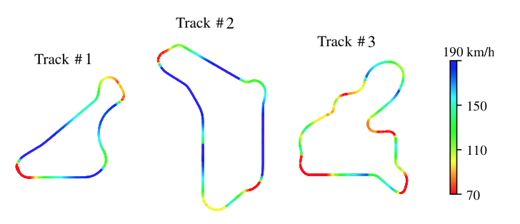
Figure 7: Speed profiles of our proposed controller on TORCS

V Conclusion

In this paper, we propose a method for the control of aggressive driving of autonomous cars, which features a modular design that is consisted of mechanism-based and data-driven components, and aware of the two-timescale phenomenon in the car model. Experiment results on a tracking task and a racing task show that our proposed method enjoys benefits over existing mechanism-based and data-driven methods in terms of data efficiency, ability of transfer and final performance.

References

- [1] M. Ryan, “The future of transportation: ethical, legal, social and economic impacts of self-driving vehicles in the year 2025,” Science and engineering ethics, pp. 1–24, 2019.
- [2] M. Campbell, M. Egerstedt, J. P. How, and R. M. Murray, “Autonomous driving in urban environments: approaches, lessons and challenges,” Philosophical Transactions of the Royal Society A: Mathematical, Physical and Engineering Sciences, vol. 368, no. 1928, pp. 4649–4672, 2010.
- [3] C. Hubmann, M. Becker, D. Althoff, D. Lenz, and C. Stiller, “Decision making for autonomous driving considering interaction and uncertain prediction of surrounding vehicles,” in 2017 IEEE Intelligent Vehicles Symposium (IV), pp. 1671–1678, IEEE, 2017.
- [4] V. Talpaert, I. Sobh, B. R. Kiran, P. Mannion, S. Yogamani, A. El-Sallab, and P. Perez, “Exploring applications of deep reinforcement learning for real-world autonomous driving systems,” arXiv preprint arXiv:1901.01536, 2019.
- [5] J. H. Jeon, S. Karaman, and E. Frazzoli, “Anytime computation of time-optimal off-road vehicle maneuvers using the RRT,” Proceedings of the IEEE Conference on Decision and Control, pp. 3276–3282, 2011.
- [6] S. Dixit, S. Fallah, U. Montanaro, M. Dianati, A. Stevens, F. Mccullough, and A. Mouzakitis, “Trajectory planning and tracking for autonomous overtaking: State-of-the-art and future prospects,” Annual Reviews in Control, vol. 45, pp. 76–86, 2018.
- [7] H. Pacejka and I. Besselink, “Magic formula tyre model with transient properties,” Vehicle system dynamics, vol. 27, no. S1, pp. 234–249, 1997.
- [8] U. Rosolia and F. Borrelli, “Learning How to Autonomously Race a Car: a Predictive Control Approach,” 2019.
- [9] L. Hewing, A. Liniger, and M. N. Zeilinger, “Cautious nmpc with gaussian process dynamics for autonomous miniature race cars,” in 2018 European Control Conference (ECC), p. 1341–1348, IEEE, Jun 2018.
- [10] B. Wymann, E. Espié, C. Guionneau, C. Dimitrakakis, R. Coulom, and A. Sumner, “Torcs, the open racing car simulator,” Software available at http://torcs. sourceforge. net, vol. 4, no. 6, 2000.
- [11] L. Biegler and V. Zavala, “Large-scale nonlinear programming using ipopt: An integrating framework for enterprise-wide dynamic optimization,” Computers & Chemical Engineering, vol. 33, p. 575–582, Mar 2009.
- [12] J. D. Lambert, Numerical methods for ordinary differential systems: the initial value problem. Wiley, 1991.
- [13] P. J. Huber, “Robust estimation of a location parameter,” in Breakthroughs in statistics, pp. 492–518, Springer, 1992.
- [14] D. C. Liu and J. Nocedal, “On the limited memory bfgs method for large scale optimization,” Mathematical Programming, vol. 45, p. 503–528, Aug 1989.
- [15] T. Haarnoja, A. Zhou, P. Abbeel, and S. Levine, “Soft actor-critic: Off-policy maximum entropy deep reinforcement learning with a stochastic actor,” arXiv:1801.01290 [cs, stat], Aug 2018. arXiv: 1801.01290.