Mini-batch stochastic Nesterov’s smoothing method for constrained convex stochastic composite optimization

Abstract

This paper considers a class of constrained convex stochastic composite optimization problems whose objective function is given by the summation of a differentiable convex component, together with a nonsmooth but convex component. The nonsmooth component has an explicit max structure that may not easy to compute its proximal mapping. In order to solve these problems, we propose a mini-batch stochastic Nesterov’s smoothing (MSNS) method. Convergence and the optimal iteration complexity of the method are established. Numerical results are provided to illustrate the efficiency of the proposed MSNS method for a support vector machine (SVM) model.

1 Introduction

In this paper, we consider the nonsmooth convex stochastic composite minimization problem

$$\psi^{*}:=\min\limits_{x\in X}\{\psi(x):=f(x)+h(x)\},$$ (1)

where $X$ is a bounded closed convex set in the Euclidean space $\mathds{R}^{n}$, $f:X\rightarrow\mathds{R}$ is a convex function with Lipschitz continuous gradient, and $h:X\rightarrow\mathds{R}$ is a possibly nonsmooth convex function with the explicit max structure

$$h(x)=\max_{u\in U}\{\langle Ax,u\rangle-Q(u)\},$$ (2)

where $U$ is a bounded closed convex set, $A$ is a linear operator, and $Q(u)$ is a continuous convex function. Such function $h$ has been studied by Nesterov Nesterov with various important applications, and its max structure has been used to construct the smoothing approximation $h_{\mu}(x)$ of $h(x)$ so that its gradient is Lipschitz continuous.

Although $f$ and $h_{\mu}$ are Lipschitz continuously differentiable, we assume that only the noisy objective values and gradients of $f$ and $h_{\mu}$ are available via subsequent calls to a stochastic oracle ($\cal SO$). Many applications especially in machine learning are in this setting. That is, when we solve the smooth problem

$$\min\limits_{x\in X}\{\psi_{\mu}(x):=f(x)+h_{\mu}(x)\},$$ (3)

by an iterative algorithm, at the $k$-th iterate, $k\geq 1$, for the input $x_{k}\in X$, the $\cal SO$ would output a stochastic value $\Psi_{\mu}(x_{k},\xi_{k})$ and a stochastic gradient $\nabla\Psi_{\mu}(x_{k},\xi_{k})$ in the form of

$$\Psi_{\mu}(x_{k},\xi_{k}):=F(x_{k},\xi_{k})+H_{\mu}(x_{k},\xi_{k})$$

and

$$\nabla\Psi_{\mu}(x_{k},\xi_{k}):=\nabla F(x_{k},\xi_{k})+\nabla H_{\mu}(x_{k},\xi_{k}),$$

where $\xi_{k}$ is a random vector whose probability distribution is supported on $\Xi\subseteq\mathds{R}^{d}$.

Assumption 1

For any fixed $\mu>0$, and $x\in X$, we have

$$a) E[\Psi_{\mu}(x,\xi)]=\psi_{\mu}(x),$$

$$b) E[\nabla\Psi_{\mu}(x,\xi)]=\nabla\psi_{\mu}(x),$$

$$c) E[\|\nabla\Psi_{\mu}(x,\xi)-\nabla\psi_{\mu}(x)\|^{2}]\leq\sigma^{2},$$

where $\sigma>0$ is a constant, and the expectation $E$ is taken with respect to the random vector $\xi\in\Xi$.

The stochastic approximation (SA) is one important approach for solving stochastic convex programming, which can be dated back to the pioneering paper by Robbins and Monro Robbins . A robust version of the SA method developed by Polyak Polyak , and Polyak and Juditsky Polyak2 , improves the original version of the SA method. It was demonstrated in Nemirovski et al. Nemirovski1 that a proper modification of the SA approach based on the mirror-descent SA (Nemirovski and Yudin Nemirovski2 ), can be competitive and can even significantly outperform the other important type approach, the sample average approximation (SAA) method Kleywegt ; Shapiro1 , for a certain class of convex stochastic programming in Lan ; Nemirovski . It has been pointed out in Nemirovski1 that for nonsmooth stochastic convex optimization, the iteration complexity of order

$$O\left(\frac{1}{\epsilon^{2}}\right)$$

is optimal, where $\epsilon$ is the desired absolute accuracy of the approximate solution in objective value. In 2016, S. Ghadimi et al. Ghadimi proposed a novel randomized stochastic projected gradient (RSPG) algorithm which can solve constrained nonconvex nonsmooth stochastic composite problems. The nonsmooth component $h$ in Ghadimi , however, is restricted to be a simple convex function such as $h(x)=\|x\|_{1}$, for which the proximal operator is easy to compute. Such restriction still exists for the other stochastic proximal type methods, e.g., Wang ; Ma ; Xiao . There are many real applications in which the nonsmooth term is not so easy to obtain the proximal operator, such as a support vector machine (SVM) model we consider in numerical experiment in Section 4, where $h$ is a maximum of $0$ and an affine function.

Smoothing methods have been shown to be efficient for dealing with constrained nonsmooth optimization with solid convergence results, which allow the nonsmooth terms to be relatively complex Nesterov ; Zhang ; Chen ; Bian ; Liu ; Zhang2 . In this paper, we propose a mini-batch stochastic Nesterov’s smoothing (MSNS) method for solving (1) with relatively complex nonsmooth convex component $h$. Note that Nesterov’s smoothing method Nesterov was designed for solving deterministic constrained convex nonsmooth composite optimization problems. The MSNS method proposed in this paper is suitable for stochastic setting. The extension, however, is not a trivial task. We show the convergence, as well as the optimal iteration complexity of the MSNS method. We illustrate the efficiency of the MSNS method, by comparing with several state-of-the-art SA-type methods, on a SVM model using both synthetic data and several real data.

The remaining part of this paper is organized as follows. In Section 2, we briefly review some basic concepts and results relating to the Nesterov’s smoothing method Nesterov that will be used in our paper. In Section 3, we develop a mini-batch stochastic Nesterov’s smoothing method which extends the Nesterov’s smoothing method from the deterministic setting to the stochastic setting. We show the convergence, as well as the optimal iteration complexity of the proposed method. Numerical experiments on a SVM model are given in Section 4 to demonstrate the efficiency of our proposed method.

2 Preliminaries

In this section, we review some basic concepts and results relating to the Nesterov’s smoothing method Nesterov that will be used later. The problem (1) can be considered as a convex-concave saddle point problem

$$\min\limits_{x\in X}\max\limits_{u\in U}\left\{K(x,u):=f(x)+\langle Ax,u\rangle-Q(u)\right\},$$

where $K$ is convex in $x$ on $X$, and concave in $u$ on $U$. The adjoint form of the problem (1) can be written as

$$\max\limits_{u\in U}\left\{\phi(u):=\min\limits_{x\in X}K(x,u)\right\}.$$ (4)

We call (1) the “primal problem” and (4) the “dual problem”. It is easy to see that

$$\psi(x)\geq\phi(u),\quad\mbox{for any}\ x\in X\ \mbox{and}\ u\in U.$$

Since the objective function of each problem is continuous and the feasible region is compact, we know that there exists $x^{*}\in X$ and $u^{*}\in U$, which are optimal solutions of (1) and (4), respectively. According to Theorem 4.2’ in Sion , we have

$$\min\limits_{x\in X}\max\limits_{u\in U}K(x,u)=\max\limits_{u\in U}\min\limits_{x\in X}K(x,u).$$

That is, $\psi(x^{*})=\phi(u^{*})$. Hence in the Nesterov’s smoothing method Nesterov for the determinstic setting, if the gap $\psi({\widehat{x}})-\phi({\widehat{u}})\leq\epsilon$ for a tolerance $\epsilon>0$, the output $\widehat{x}$ is called an $\epsilon$-approximate solution of the primal problem (1).

As in Nesterov , by inserting a non-negative, continuous and $\sigma_{\omega}$-strongly convex function $\omega(u)$ in (2), we obtain a smooth approximation $h_{\mu}(x)$ of $h(x)$

$$h_{\mu}(x):=\max\limits_{u\in U}\left\{\langle Ax,u\rangle-Q(u)-\mu\omega(u)\right\},$$ (5)

where $\mu>0$ is a smoothing parameter. Let us denote by $u_{\mu}(x)$ the optimal solution of the above problem. Recall that $\omega(u)$ is strongly convex on $U$ if there exists a constant $\sigma_{\omega}>0$ such that

$$\omega(u_{1})\geq\omega(u_{2})+\left\langle\nabla\omega(u_{2}),u_{1}-u_{2}\right\rangle+\frac{1}{2}\sigma_{\omega}\|u_{1}-u_{2}\|^{2},~{}~{}\forall u_{1},u_{2}\in U.$$ (6)

Denote by $u_{0}=\arg\min\limits_{u\in U}\{\omega(u)\}$. Without loss of generality we assume that $\omega(u_{0})=0$. By (6), for any $u\in U$ we have

$$\omega(u)\geq\frac{1}{2}\sigma_{\omega}\|u-u_{0}\|^{2}.$$ (7)

Let $\Omega=\max\limits_{u\in U}\{\omega(u)\}$. Then, according to Nesterov , for any $x\in X$ we have

$$h_{\mu}(x)\leq h(x)\leq h_{\mu}(x)+\mu\Omega.$$ (8)

Lemma 1

(Theorem 1 of Nesterov ) The function $h_{\mu}(x)$ is well defined and continuously differentiable at any $x\in X$. Moreover, this function is convex and its gradient

$$\nabla h_{\mu}(x)=A^{T}u_{\mu}(x)$$

is Lipschitz continuous with constant

$$L_{h_{\mu}}=\frac{1}{\mu\sigma_{\omega}}\|A\|^{2},$$ (9)

where $\|A\|$ is the operator norm of $A$.

We then find $\psi_{\mu}(x)$ is $L$-smooth on $X$, i.e., $\psi_{\mu}(x)$ is Lipschitz continuously differentiable with Lipschitz constant $0<L=L_{f}+L_{h_{\mu}}$ on $X$. According to Theorem 5.12 of Beck , we get $L_{f}\geq\|\nabla^{2}f(x)\|=\lambda_{\max}(\nabla^{2}f(x))$ for any $x\in X$, where $\lambda_{\max}(\nabla^{2}f(x))$ means the maximal eigenvalue of the Hessian matrix of $f(x)$. Thus

$$\psi_{\mu}(y)\leq\psi_{\mu}(x)+\langle\nabla\psi_{\mu}(x),y-x\rangle+\frac{L}{2}\|y-x\|^{2},\quad\forall x,y\in X.$$ (10)

Let $d(x)$ be a prox-function of the set $X$. We assume that $d(x)$ is continuous and strongly convex on $X$ with convexity parameter $\sigma_{d}>0$. Let $x_{0}$ be the center of the set $X$, i.e., $x_{0}=\arg\min\{d(x):x\in X\}$. Without loss of generality we assume that $d(x_{0})=0$. Thus

$$d(x)\geq\frac{1}{2}\sigma_{d}\|x-x_{0}\|^{2}.$$ (11)

In view of the compact set $X$, we know that there exists a constant $D>0$ such that

$$\max\limits_{x\in X}\{d(x)\}\leq D.$$ (12)

Given $g\in\mathds{R}^{n}$, we define the generalized projected gradient of $\psi$ at $x\in X$ as

$$P_{X}(x,g,\gamma)=\frac{1}{\gamma}(x-x^{\prime}),$$ (13)

where $x^{\prime}$ is given by

$$x^{\prime}=\arg\min\limits_{y\in X}\left\{\langle g,y\rangle+\frac{1}{2\gamma}\|y-x\|^{2}\right\}.$$ (14)

Lemma 2

Let $P_{X}(x,g,\gamma)$ be defined in (13)-(14). Then, for any $x\in X$, $\mu>0$ and $\gamma>0$, the stochastic gradient $\nabla\Psi_{\mu}(x,\xi)$ and the full gradient $\nabla\psi_{\mu}(x)$ satisfy

$$\|P_{X}(x,\nabla\Psi_{\mu}(x,\xi),\gamma)-P_{X}(x,\nabla\psi_{\mu}(x),\gamma)\|\leq\|\nabla\Psi_{\mu}(x,\xi)-\nabla\psi_{\mu}(x)\|.$$ (15)

Proof

The generalized projected gradient defined in (13)-(14) is a special case of that defined in (2.3)-(2.4) of Ghadimi , with $V(y,x)=1/2\|y-x\|^{2}$, the convexity parameter $\alpha=1$, and $h(x)=0$ in (2.3) of Ghadimi . Then the statement in this lemma can be obtained easily from Proposition 1 of Ghadimi , which claims that the generalized projected gradient $P_{X}(x,\cdot,\gamma)$ is Lipschitz continuous with Lipschitz constant $1/{\alpha}=1$.

3 Mini-batch Stochastic Nesterov’s Smoothing Method

In this section, we develop a novel mini-batch stochastic Nesterov’s smoothing (MSNS) method for solving (1). We will show the convergence as well as the optimal iteration complexity of the MSNS method.

At the $k$-th iterate of the MSNS method, we randomly choose a mini-bath samples $\xi^{[m_{k}]}:=\{\xi_{k,1},\ldots,\xi_{k,m_{k}}\}$ of the random vector $\xi\in\Xi$, where $m_{k}$ is the batch size. And we denote by $\xi_{[k]}:=\{\xi^{[m_{0}]},\ldots,\xi^{[m_{k}]}\}$ the history of mini-batch samples from the $0$-th iterate up to the $k$-th iterate. For any $k\geq 0$, we denote the mini-batch stochastic objective value $\Psi_{\mu}^{k}$, and the mini-batch stochastic gradient $\nabla\Psi_{\mu}^{k}$ by

$$\Psi_{\mu}^{k}=\frac{1}{m_{k}}\sum\limits_{j=1}^{m_{k}}\Psi_{\mu}(x_{k},\xi_{k,j}),\quad\nabla\Psi_{\mu}^{k}=\frac{1}{m_{k}}\sum\limits_{j=1}^{m_{k}}\nabla\Psi_{\mu}(x_{k},\xi_{k,j}).$$ (16)

For ease of notations in the proof, we denote

$$\delta_{\mu}(x_{k}):=\nabla\Psi_{\mu}^{k}-\nabla\psi_{\mu}(x_{k}),$$ (17)

$$\delta_{\mu}^{i}(x_{k}):=\nabla\Psi_{\mu}(x_{k},\xi_{k,i})-\nabla\psi_{\mu}(x_{k}),\ i=1,\cdots,m_{k},$$ (18)

$$S_{\mu}^{j}(x_{k}):=\sum\limits_{i=1}^{j}\delta_{\mu}^{i}(x_{k}),\ j=1,\cdots,m_{k}.$$ (19)

The following lemma addresses the relations of $\Psi_{\mu}^{k}$ and $\nabla\Psi_{\mu}^{k}$ to that of the original objective value $\psi_{\mu}(x_{k})$ and $\nabla\psi_{\mu}(x_{k})$, which can be shown without difficulty using the arguments similar as in Ghadimi .

Lemma 3

Under Assumption 1, we have for any $k\geq 0$ and $\mu>0$,

$$(a) E\left[\Psi_{\mu}^{k}\right]=E\left[\psi_{\mu}(x_{k})\right],$$

$$(b) E\left[\nabla\Psi_{\mu}^{k}\right]=E[\nabla\psi_{\mu}(x_{k})],$$

$$(c) E\left[\|\nabla\Psi_{\mu}^{k}-\psi_{\mu}(x_{k})\|^{2}\right]\leq\frac{\sigma^{2}}{m_{k}},$$

where the expectation is taken with respect to the history of mini-batch samples $\xi_{[k]}$.

Proof

Note that the $k$-th iterate $x_{k}$ is a function of the history $\xi_{[k-1]}$ of the generated random process and consequently is random, and it is independent of the mini-batch samples $\xi^{[m_{k}]}$ at the $k$-th iterate.

For $k=0$, no history of mini-batch samples to call the $\cal SO$ exists before this iterate. Thus Lemma 3 can be obtained immediately using Assumption 1.

Now we consider the case for any $k\geq 1$. Using Assumption 1 (a), we have

$$E\left[\Psi_{\mu}^{k}\right] = E\left\{E\left[\Psi_{\mu}^{k}|\xi_{[k-1]}\right]\right\}$$

$$\overset{\eqref{eq3.9}}{=} E\left\{E\left[\frac{1}{m_{k}}\sum\limits_{j=1}^{m_{k}}\Psi_{\mu}(x_{k},\xi_{k,j})|\xi_{[k-1]}\right]\right\}$$

$$= E\left\{\frac{1}{m_{k}}\sum\limits_{j=1}^{m_{k}}E\left[\Psi_{\mu}(x_{k},\xi_{k,j})|\xi_{[k-1]}\right]\right\}$$

$${=} E\left[\psi_{\mu}(x_{k})\right].$$

Employing Assumption 1 (b), we get

$$E\left[\nabla\Psi_{\mu}^{k}\right] = E\left\{E\left[\nabla\Psi_{\mu}^{k}|\xi_{[k-1]}\right]\right\}$$

$$\overset{\eqref{eq3.9}}{=} E\left\{E\left[\frac{1}{m_{k}}\sum\limits_{j=1}^{m_{k}}\nabla\Psi_{\mu}(x_{k},\xi_{k,j})|\xi_{[k-1]}\right]\right\}$$

$$= E\left\{\frac{1}{m_{k}}\sum\limits_{j=1}^{m_{k}}E\left[\nabla\Psi_{\mu}(x_{k},\xi_{k,j})|\xi_{[k-1]}\right]\right\}$$

$${=} E\left[\nabla\psi_{\mu}(x_{k})\right].$$

Thus Lemma 3 (a) and (b) hold. Lemma 3 (c) can be deduced from the proof of (4.12) in Theorem 2 Ghadimi , by noticing the definitions of $\delta_{\mu}^{i}(x_{k})$ and $S^{i-1}_{\mu}(x_{k})$ in (18) and (19), respectively.

In our scheme we update recursively three sequences of points $\{x_{k}\}_{k=0}^{\infty}$, $\{y_{k}\}_{k=0}^{\infty}$ and $\{z_{k}\}_{k=0}^{\infty}$ in $X$. To be specific, given an initial point $x_{0}\in X$, a fixed smoothing parameter $\mu>0$, a sequence of mini-batch sizes $\{m_{k}\}_{k=0}^{\infty}$, and sequences of positive real numbers $\{\gamma_{k}\}_{k=0}^{\infty}$, $\{\alpha_{k}\}_{k=0}^{\infty}$ and $\{\tau_{k}\}_{k=0}^{\infty}$, then for $k\geq 0$ we recursively obtain

$$y_{k} = \arg\min\limits_{y\in X}\left\{\ell^{k}(y):=\langle\nabla\Psi_{\mu}^{k},y-x_{k}\rangle+\frac{1}{2\gamma_{k}}\|y-x_{k}\|^{2}\right\},$$ (20)

$$z_{k} = \arg\min\limits_{x\in X}\left\{\pi^{k}(x):=\frac{L}{\sigma_{d}}d(x)+\sum\limits_{i=0}^{k}\alpha_{i}\left[\Psi_{\mu}^{i}+\langle\nabla\Psi_{\mu}^{i},x-x_{i}\rangle\right]\right\},$$ (21)

$$x_{k+1} = \tau_{k}z_{k}+(1-\tau_{k})y_{k}.$$ (22)

Let us denote

$$B_{i}:=\dfrac{\sqrt{A_{i}}\sigma^{2}}{m_{i}L},\quad C_{i}:=\dfrac{LA_{i}(1-\sqrt{A_{i}})}{2}\|y_{i}-x_{i}\|^{2},$$ (23)

and

$$\Gamma_{k}(x):=E\left[\pi^{k}(x)\right]+\sum\limits_{i=0}^{k}B_{i}+E\left[\sum\limits_{i=0}^{k}C_{i}\right],\quad\quad$$ (24)

where the expectation is taken with respect to the history of mini-batch samples $\xi_{[k]}$. By selecting proper positive sequences $\{\gamma_{k}\}_{k=0}^{\infty}$, $\{\alpha_{k}\}_{k=0}^{\infty}$ and $\{\tau_{k}\}_{k=0}^{\infty}$, we then have the following proposition.

Proposition 1

Let some sequence $\{\alpha_{k}\}_{k=0}^{\infty}$ satisfy the condition:

$$\alpha_{0}\in(0,1],~{}~{}\alpha_{k}>0,~{}~{}\alpha_{k+1}^{2}\leq\sqrt{A_{k+1}},$$ (25)

where $A_{k}=\sum\limits_{i=0}^{k}\alpha_{i}$. Let us choose $\tau_{k}=\frac{\alpha_{k+1}}{A_{k+1}}$, $\gamma_{k}=\frac{1}{L\sqrt{A_{k}}}$. Then for any $k\geq 0$,

$$\quad\quad\quad\quad\quad\quad\quad\quad A_{k}E[\psi_{\mu}(y_{k})]\leq\min\left\{\Gamma_{k}(x)\ :\ x\in X\right\},\quad\quad\quad\quad\quad\quad(\mathcal{R}_{k})$$

where $\Gamma_{k}$ is defined in (24) and the expectation is taken with respect to $\xi_{[k]}$.

Proof

For any $k\geq 0$, using Lemma 2 and the definition of $\delta_{\mu}(x_{k})$ in (17),

$$\left\langle\delta_{\mu}(x_{k}),P_{X}(x_{k},\nabla\Psi_{\mu}^{k},\gamma_{k})-P_{X}(x_{k},\nabla\psi_{\mu}(x_{k}),\gamma_{k})\right\rangle$$

$$~{}~{}~{}\leq~{}\|\delta_{\mu}(x_{k})\|\|P_{X}(x_{k},\nabla\Psi_{\mu}^{k},\gamma_{k})-P_{X}(x_{k},\nabla\psi_{\mu}(x_{k}),\gamma_{k})\|$$

$$~{}\overset{\eqref{Pleqg}}{\leq}\|\delta_{\mu}(x_{k})\|\|\nabla\Psi_{\mu}^{k}-\nabla\psi_{\mu}(x_{k})\|=~{}\|\delta_{\mu}(x_{k})\|^{2},$$

and

$$E\left[\left\langle\delta_{\mu}(x_{k}),P_{X}(x_{k},\nabla\psi_{\mu}(x_{k}),\gamma_{k})\right\rangle\right]$$

$$~{}=E\left\{E\left[\left\langle\delta_{\mu}(x_{k}),P_{X}(x_{k},\nabla\psi_{\mu}(x_{k}),\gamma_{k})\right\rangle|\xi_{[k-1]}\right]\right\}$$

$$~{}=E\left\{\left\langle E\left[\delta_{\mu}(x_{k})|\xi_{[k-1]}\right],P_{X}(x_{k},\nabla\psi_{\mu}(x_{k}),\gamma_{k})\right\rangle\right\}$$

$$~{}=E\left\{\left\langle E\left[\left(\nabla\Psi_{\mu}^{k}-\nabla\psi_{\mu}(x_{k})\right)|\xi_{[k-1]}\right],P_{X}(x_{k},\nabla\psi_{\mu}(x_{k}),\gamma_{k})\right\rangle\right\}=0.$$

Therefore, for any $k\geq 0$,

$$A_{k}E\left[\langle\delta_{\mu}(x_{k}),x_{k}-y_{k}\rangle\right]$$ (26)

$$~{}~{}=\frac{\sqrt{A_{k}}}{L}E\left[\langle\delta_{\mu}(x_{k}),P_{X}(x_{k},\nabla\Psi_{\mu}^{k},\gamma_{k})\rangle\right]$$

$$~{}~{}=\frac{\sqrt{A_{k}}}{L}E\left[\langle\delta_{\mu}(x_{k}),P_{X}(x_{k},\nabla\Psi_{\mu}^{k},\gamma_{k})-P_{X}(x_{k},\nabla\psi_{\mu}(x_{k}),\gamma_{k})\rangle\right]$$

$$~{}~{}~{}~{}~{}~{}~{}~{}~{}+\frac{\sqrt{A_{k}}}{L}E\left[\langle\delta_{\mu}(x_{k}),P_{X}(x_{k},\nabla\psi_{\mu}(x_{k}),\gamma_{k})\rangle\right]$$

$$~{}~{}\leq\frac{\sqrt{A_{k}}}{L}E\left[\|\delta_{\mu}(x_{k})\|^{2}\right]\leq B_{k},$$

where the last inequality comes from Lemma 3 (c) and the definition of $B_{k}$ in (23).

Now we prove the theorem by mathematical induction. For $k=0$, in terms of Lemma 3 for the first equality below, we have for any $x\in X$ and $\mu>0$,

$$A_{0}E\left[\psi_{\mu}(y_{0})\right]\quad\quad\quad\quad\quad\quad\quad$$

$$~{}\overset{\eqref{eq3.10}}{\leq}A_{0}E\left[\psi_{\mu}(x_{0})+\langle\nabla\psi_{\mu}(x_{0}),y_{0}-x_{0}\rangle+\frac{L}{2}\|y_{0}-x_{0}\|^{2}\right]$$

$$~{}\overset{\eqref{notation2-1}}{=}A_{0}E\left[\Psi_{\mu}^{0}+\langle\nabla\Psi_{\mu}^{0},y_{0}-x_{0}\rangle+\frac{L}{2}\|y_{0}-x_{0}\|^{2}\right]+A_{0}E\left[\langle\delta_{\mu}(x_{0}),x_{0}-y_{0}\rangle\right]$$

$$~{}\overset{\eqref{theorem-1-result-1}}{\leq}A_{0}E\left[\Psi_{\mu}^{0}+\ell^{0}(y_{0})\right]+C_{0}+B_{0},$$

where the definition of $\ell^{0}(y_{0})$ can be found in (20). Using the formula to obtain $y_{0}$ in (20), we have for any $x\in X$,

$$\ell^{0}(y_{0})\leq\ell^{0}(x)=\langle\nabla\Psi_{\mu}^{0},x-x_{0}\rangle+\frac{1}{2\gamma_{0}}\|x-x_{0}\|^{2}.$$ (27)

Noting that $A_{0}=\alpha_{0}\in(0,1]$, $\gamma_{0}=\frac{1}{L\sqrt{A_{0}}}$, and (11), we find the second term in the right-hand side of the equation in (27) satisfies

$$\frac{1}{2\gamma_{0}}\|x-x_{0}\|^{2}=\frac{L\sqrt{A_{0}}}{2}\|x-x_{0}\|^{2}\leq\frac{L}{\sigma_{d}}d(x).$$ (28)

Therefore, by using (27), (28), and the definition of $\pi^{0}(x)$ obtained by (21), we get

$$A_{0}\left[\Psi_{\mu}^{0}+\ell^{0}(y_{0})\right]\leq\frac{L}{\sigma_{d}}d(x)+\alpha_{0}\left[\Psi_{\mu}^{0}+\langle\nabla\Psi_{\mu}^{0},x-x_{0}\rangle\right]=\pi^{0}(x).$$

With these observations, we have $(\mathcal{R}_{0})$ holds.

Assume $(\mathcal{R}_{k})$ holds. By the formula for obtaining $z_{k}$ in (21), the optimality condition of the minimization problem in (21) at $z_{k}$ gives

$$-\frac{L}{\sigma_{d}}\langle\nabla d(z_{k}),x-z_{k}\rangle\leq\sum\limits_{i=0}^{k}\alpha_{i}\left\langle\nabla\Psi_{\mu}^{i},x-z_{k}\right\rangle.$$ (29)

This, together with the strong convexity of the function $d$ with the convexity parameter $\sigma_{d}$, yields

$$\frac{L}{\sigma_{d}}\left[d(z_{k})+\frac{\sigma_{d}}{2}\|x-z_{k}\|^{2}\right] \leq \frac{L}{\sigma_{d}}\left[d(x)-\left\langle\nabla d(z_{k}),x-z_{k}\right\rangle\right]$$ (30)

$$\overset{\eqref{argu1}}{\leq} \frac{L}{\sigma_{d}}d(x)+\sum_{i=0}^{k}\alpha_{i}\left\langle\nabla\Psi_{\mu}^{i},x-z_{k}\right\rangle.$$

By noting the objective function $\pi_{k}$ of the minimization problem to find $z_{k}$ in (21), we know

$$\pi^{k+1}(x)=\pi^{k}(x)+\alpha_{k+1}\left[\Psi_{\mu}^{k+1}+\langle\nabla\Psi_{\mu}^{k+1},x-x_{k+1}\rangle\right],$$ (31)

and

$$\pi^{k}(x) = \frac{L}{\sigma_{d}}d(x)+\sum_{i=0}^{k}\alpha_{i}\left[\Psi_{\mu}^{i}+\langle\nabla\Psi_{\mu}^{i},x-x_{i}\rangle\right]$$ (32)

$$= \frac{L}{\sigma_{d}}d(x)+\sum_{i=0}^{k}\alpha_{i}\langle\nabla\Psi_{\mu}^{i},x-z_{k}\rangle+\sum_{i=0}^{k}\alpha_{i}\left[\Psi_{\mu}^{i}+\langle\nabla\Psi_{\mu}^{i},z_{k}-x_{i}\rangle\right]$$

$$\overset{\eqref{proof-statement-2}}{\geq} \frac{L}{\sigma_{d}}\left[d(z_{k})+\frac{\sigma_{d}}{2}\|x-z_{k}\|^{2}\right]+\sum_{i=0}^{k}\alpha_{i}\left[\Psi_{\mu}^{i}+\langle\nabla\Psi_{\mu}^{i},z_{k}-x_{i}\rangle\right]$$

$$= \pi^{k}(z_{k})+\frac{L}{2}\|x-z^{k}\|^{2}.$$

Let us denote

$$T^{k+1} := \alpha_{k+1}\left[\Psi_{\mu}^{k+1}+\langle\nabla\Psi_{\mu}^{k+1},x-x_{k+1}\rangle\right],$$ (33)

$$t^{k+1} := \alpha_{k+1}\left[\psi_{\mu}(x_{k+1})+\langle\nabla\psi_{\mu}(x_{k+1}),x-x_{k+1}\rangle\right].$$ (34)

It is clear that $E\left[T^{k+1}\right]=E\left[t^{k+1}\right]$ by Lemma 3. Combining (31) and (32), we have

$$\pi^{k+1}(x)\geq\pi^{k}(z_{k})+\frac{L}{2}\|x-z_{k}\|^{2}+T^{k+1}.$$ (35)

Therefore, for any $x\in X$,

$$\Gamma_{k+1}(x) = E\left[\pi^{k+1}(x)\right]+\sum_{i=0}^{k+1}B_{i}+E\left[\sum_{i=0}^{k+1}C_{i}\right]$$ (36)

$$\overset{\eqref{proof-statement-3}}{\geq} E\left[\pi^{k}(z_{k})+\frac{L}{2}\|x-z^{k}\|^{2}+T^{k+1}\right]+\sum_{i=0}^{k+1}B_{i}+E\left[\sum_{i=0}^{k+1}C_{i}\right]$$

$$= \Gamma_{k}(z_{k})+E\left[T^{k+1}\right]+\frac{L}{2}E\left[\|x-z_{k}\|^{2}\right]+B_{k+1}+E\left[C_{k+1}\right].~{}~{}$$

For the summation of the first two terms in (36), we have

$$\Gamma_{k}(z_{k})+E\left[T^{k+1}\right]$$

$$\quad\geq A_{k}E\left[\psi_{\mu}(y_{k})\right]+E\left[t^{k+1}\right]$$

$$\quad\geq A_{k}E\left[\psi_{\mu}(x_{k+1})+\langle\nabla\psi_{\mu}(x_{k+1}),y_{k}-x_{k+1}\rangle\right]+E\left[t^{k+1}\right]$$

$$\quad=A_{k+1}E\left[\psi_{\mu}(x_{k+1})\right]+E\left[\langle\nabla\psi_{\mu}(x_{k+1}),A_{k}y_{k}-A_{k+1}x_{k+1}+\alpha_{k+1}x\rangle\right].\quad\quad\quad$$ (37)

Here the first inequality comes form the assumption $({\cal R}_{k})$ holds, and the fact that $E[T^{k+1}]=E[t^{k+1}]$, and the second inequality is obtained from the convexity of $\psi_{\mu}$, and the first equality is obtained by using the definition of $t^{k+1}$ in (34), and the choice of $A_{k}$ such that $A_{k+1}=A_{k}+\alpha_{k+1}$. Furthermore, for the second term of $\langle\cdot,\cdot\rangle$ in (3), by noting $\tau_{k}=\frac{\alpha_{k+1}}{A_{k+1}}$, $1-\tau_{k}=\frac{A_{k}}{A_{k+1}}$, and $x_{k+1}=\tau_{k}z_{k}+(1-\tau_{k})y_{k}$ in (22), we have

$$A_{k}y_{k}-A_{k+1}x_{k+1}+\alpha_{k+1}x = A_{k}y_{k}-\alpha_{k+1}z_{k}-A_{k+1}\frac{A_{k}}{A_{k+1}}y_{k}+\alpha_{k+1}x$$ (38)

$$= \alpha_{k+1}(x-z_{k})=A_{k+1}\tau_{k}(x-z_{k}).$$

In view of $\tau_{k}=\frac{\alpha_{k+1}}{A_{k+1}}$ and $\alpha_{k+1}^{2}\leq\sqrt{A_{k+1}}$, we know

$$\frac{1}{A_{k+1}}\geq\tau_{k}^{2}\sqrt{A_{k+1}}.$$ (39)

Using (36) – (39), we find

$$\Gamma_{k+1}(x)$$

$$~{}~{}\geq A_{k+1}E\left[\psi_{\mu}(x_{k+1})\right]+A_{k+1}\tau_{k}E\left[\langle\nabla\psi_{\mu}(x_{k+1}),x-z_{k}\rangle\right]+\frac{L}{2}E\left[\|x-z_{k}\|^{2}\right]$$

$$~{}~{}~{}~{}~{}~{}~{}~{}+B_{k+1}+E\left[C_{k+1}\right]$$

$$~{}\overset{\eqref{coefficient}}{\geq}A_{k+1}E\left[\psi_{\mu}(x_{k+1})+\tau_{k}\langle\nabla\psi_{\mu}(x_{k+1}),x-z_{k}\rangle+\frac{L\tau_{k}^{2}\sqrt{A_{k+1}}}{2}\|x-z_{k}\|^{2}\right]$$

$$~{}~{}~{}~{}~{}~{}~{}~{}+B_{k+1}+E\left[C_{k+1}\right].$$ (40)

For any $x\in X$, let $y(x,k):=\tau_{k}x+(1-\tau_{k})y_{k}$. By using $x_{k+1}=\tau_{k}z_{k}+(1-\tau_{k})y_{k}$ in (22), we get

$$y(x,k)-x_{k+1}=\tau_{k}(x-z_{k}),$$

and consequently

$$\ell^{k+1}\left(y(x,k)\right) = \langle\nabla\Psi_{\mu}^{k+1},y(x,k)-x_{k+1}\rangle+\frac{1}{2\gamma_{k+1}}\|y(x,k)-x_{k+1}\|^{2}$$ (41)

$$= \tau_{k}\langle\nabla\Psi_{\mu}^{k+1},x-z_{k}\rangle+\frac{L\tau_{k}^{2}\sqrt{A_{k+1}}}{2}\|x-z_{k}\|^{2}.$$

Note that $x$ and $z_{k}$ are deterministic if the history of mini-batch samples $\xi_{[k]}$ is given. Thus

$$E[\langle\nabla\Psi_{\mu}^{k+1},x-z_{k}\rangle] = E\{E[\langle\nabla\Psi_{\mu}^{k+1},x-z_{k}\rangle\mid_{\xi_{[k]}}]\}$$ (42)

$$= E\{\langle E[\nabla\Psi_{\mu}^{k+1}]\mid_{\xi_{[k]}},x-z_{k}\rangle]\}$$

$$= E[\langle\nabla\psi_{\mu}(x_{k+1}),x-z_{k}\rangle].$$

Therefore, by combining (3), (41), (42) and using $E[\psi_{\mu}(x_{k+1})]=E[\Psi_{\mu}^{k+1}]$ according to Lemma 3 (a), we find

$$\Gamma_{k+1}(x)\geq A_{k+1}E\left[\Psi_{\mu}^{k+1}+\ell^{k+1}(y(x,k))\right]+B_{k+1}+E\left[C_{k+1}\right].$$ (43)

On the other hand,

$$A_{k+1}E\left[\psi_{\mu}(y_{k+1})\right]$$

$$~{}\overset{\eqref{eq3.10}}{\leq}A_{k+1}E\left[\psi_{\mu}(x_{k+1})+\langle\nabla\psi_{\mu}(x_{k+1}),y_{k+1}-x_{k+1}\rangle+\frac{L}{2}\|y_{k+1}-x_{k+1}\|^{2}\right]$$

$$~{}~{}~{}=A_{k+1}E\left[\Psi_{\mu}^{k+1}+\langle\nabla\Psi_{\mu}^{k+1}-\delta_{\mu}(x_{k+1}),y_{k+1}-x_{k+1}\rangle+\frac{L}{2}\|y_{k+1}-x_{k+1}\|^{2}\right]$$

$$~{}~{}~{}=A_{k+1}E\left[\Psi_{\mu}^{k+1}+\ell^{k+1}(y_{k+1})\right]+A_{k+1}E\left[\langle\delta_{\mu}(x_{k+1}),x_{k+1}-y_{k+1}\rangle\right]$$

$$~{}~{}~{}~{}~{}~{}~{}\quad\quad+E\left[A_{k+1}(\frac{L}{2}-\frac{1}{2\gamma_{k+1}})\|y_{k+1}-x_{k+1}\|^{2}\right]$$

$$~{}\overset{\eqref{theorem-1-result-1}}{\leq}A_{k+1}E\left[\Psi_{\mu}^{k+1}+\ell^{k+1}(y(x,k))\right]+B_{k+1}+E\left[C_{k+1}\right],$$ (44)

where the first equality is deduced by using Lemma 3 (a), and the definition of $\delta_{\mu}(x_{k+1})$, and the last inequality is obtained due to $y_{k+1}=\arg\min\limits_{y\in X}\left\{\ell^{k+1}(y)\right\}$, (26), $\gamma_{k+1}=\frac{1}{L\sqrt{A_{k+1}}}$, and the definition for $C_{k+1}$ in (23). It is easy to see from (43) and (44) that $A_{k+1}E[\psi_{\mu}(y_{k+1})]\leq\min\{\Gamma_{k+1}(x)\ :\ x\in X\}$. That is, (${\cal R}_{k+1}$) holds.

Therefore, by using mathematical induction, the relation $(\mathcal{R}_{k})$ holds for any $k\geq 0$.

Clearly, there are many ways to satisfy the conditions (25). Here we choose the special $\alpha_{k}$ and batch sizes $m_{k}$ for $k\geq 0$ as follows in order to guarantee the optimal iteration complexity of the min-batch stochastic Nesterov’s smoothing method we propose later.

Corollary 1

For $k\geq 0$ define $\alpha_{k}\equiv\frac{1}{2}$. Then

$$A_{k}=\sum\limits_{i=0}^{k}\alpha_{i}=\frac{k+1}{2},\ \tau_{k}=\frac{\alpha_{k+1}}{A_{k+1}}=\frac{1}{k+2},$$

and the conditions in (25) are satisfied. If in addition, the batch sizes $m_{k}\equiv m\geq 1$ for $k=0,\ldots,N$, then

$$E[\psi_{\mu}(y_{N})] \leq \min\limits_{x\in X}\left\{\sum\limits_{i=0}^{N}\frac{1}{N+1}E\left[\psi_{\mu}(x_{i})+\langle\nabla\psi_{\mu}(x_{i}),x-x_{i}\rangle\right]\right\}$$ (45)

$$~{}\quad+\ \frac{(6-\sqrt{2})LD}{2(N+1)\sigma_{d}}+\frac{\sqrt{2(N+1)}\sigma^{2}}{mL}.$$

Proof

Indeed, $\alpha_{k+1}^{2}=\frac{1}{4}\leq\sqrt{\frac{k+2}{2}}=\sqrt{A_{k+1}}$ for all $k\geq 0$, and consequently conditions in (25) are satisfied. For the special choices of $\alpha_{k}$ and $m_{k}$ of this corollary, we immediately get $A_{i}=\frac{i+1}{2}$,

$$\sum_{i=0}^{N}B_{i}=\sum_{i=0}^{N}\frac{\sqrt{A_{i}}\sigma^{2}}{mL}\leq\frac{(N+1)\sqrt{N+1}\sigma^{2}}{\sqrt{2}mL},$$

and

$$\sum_{i=1}^{N}C_{i} = \sum_{i=0}^{N}\frac{LA_{i}(1-\sqrt{A_{i}})}{2}\|y_{i}-x_{i}\|^{2}$$

$$\leq \frac{LA_{0}(1-\sqrt{A_{0}})}{2}\|y_{0}-x_{0}\|^{2}\leq\frac{(2-\sqrt{2})LD}{4\sigma_{d}},$$

where the first inequality holds, since $1-\sqrt{A_{i}}\leq 0$ for all $i\geq 1$, and the second inequality holds, since (11) and (12) implies

$$\frac{1}{2}\sigma_{d}\|y_{0}-x_{0}\|^{2}\leq d(y_{0})\leq D.$$

According to Proposition 1, $({\cal R}_{N})$ holds. Moreover, by using (12), we have

$${}\frac{2}{N+1}\frac{L}{\sigma_{d}}d(x)\leq 4\frac{LD}{2\sigma_{d}(N+1)}.$$ (46)

Because $x_{i}$ relates only to $\xi_{[i-1]}$, and $\nabla\Psi_{\mu}^{i}$ relates to $\xi_{[i]}$, we get by Lemma 3 that

$$E[\Psi_{\mu}^{i}]=E[\psi_{\mu}(x_{i})],\quad\mbox{and}\quad E[\langle\nabla\Psi_{\mu}^{i},x-x_{i}\rangle]=E[\langle\nabla\psi_{\mu}(x_{i}),x-x_{i}\rangle],$$ (47)

Therefore,

$$E[\psi_{\mu}(y_{N})] ~{}\overset{({\cal R}_{N})}{\leq} \min_{x\in X}\frac{2}{N+1}E\left\{\frac{L}{\sigma_{d}}d(x)+\sum_{i=0}^{N}\frac{1}{2}[\Psi_{\mu}^{i}+\langle\nabla\Psi_{\mu}^{i},x-x_{i}\rangle]\right\}$$

$$\quad\quad+\frac{\sqrt{2(N+1)}\sigma^{2}}{mL}+\frac{(2-\sqrt{2})LD}{2\sigma_{d}(N+1)},$$

and consequently we get (45) as we desired, by further noting (46), and the equalities in (47).

We are ready to give the mini-batch stochastic Nesterov’s smoothing method as follows.

Algorithm 1 Given initial point $x_{0}\in X$, iteration limit $N$, the batch sizes $m_{k}\equiv m>0$ for all $k$.
For $k=0:{N}$ do
     1. Call the $\cal SO$ $m_{k}$ times to obtain $\Psi_{\mu}(x_{k},\xi_{k,i})$ and $\nabla\Psi_{\mu}(x_{k},\xi_{k,i})$, $i=1,\cdots$,
        $m_{k}$, and set
               $\Psi_{\mu}^{k}=\frac{1}{m_{k}}\sum\limits_{i=1}^{m_{k}}\Psi_{\mu}(x_{k},\xi_{k,i})$, $\nabla\Psi_{\mu}^{k}=\frac{1}{m_{k}}\sum\limits_{i=1}^{m_{k}}\nabla\Psi_{\mu}(x_{k},\xi_{k,i})$.
     2. Find $y_{k}=\arg\min\limits_{y\in X}\left\{\langle\nabla\Psi_{\mu}^{k},y-x_{k}\rangle+\frac{L\sqrt{k+1}}{2\sqrt{2}}\|y-x_{k}\|^{2}\right\}$.
     3. Find $z_{k}=\arg\min\limits_{x\in X}\left\{\frac{L}{\sigma_{d}}d(x)+\sum\limits_{i=0}^{k}\frac{1}{2}\left[\Psi_{\mu}^{i}+\langle\nabla\Psi_{\mu}^{i},x-x_{i}\rangle\right]\right\}$.
     4. Set $x_{k+1}=\frac{1}{k+2}z_{k}+\frac{k+1}{k+2}y_{k}$.
Output: $y_{N}$.

Recall that $u_{\mu}(x)$ is the unique optimal solution of

$$\max_{u\in U}\left\{\langle Ax,u\rangle-Q(u)-\mu\omega(u)\right\}.$$

We will use $u_{\mu}(x)$ in the convergence theorem of the mini-batch stochastic Nesterov’s smoothing method.

Theorem 3.1

Let us apply Algorithm 1 to the smooth problem $\min\limits_{x\in X}\psi_{\mu}(x)$ with the following value of smoothing parameter:

$$\mu=\mu(N)=\frac{\|A\|^{2}\sqrt{(6-\sqrt{2})mD}}{\sqrt{2(N+1)\sigma_{d}\sigma_{\omega}}\sqrt{m\|A\|^{2}\Omega+\sqrt{2(N+1)}\sigma_{\omega}\sigma^{2}}},$$ (48)

where the batch size $m$ is given by

$$m=\left\lceil\frac{\sqrt{2}\sigma^{2}\sigma_{\omega}\sqrt{N+1}}{\|A\|^{2}\Omega}\right\rceil.$$ (49)

Here $\lceil\beta\rceil$ means the smallest integer that is no less than a given $\beta>0$. Then after $N$ iterations we can generate the approximate solution $\widehat{x}=y_{N}$ to the original problem (1) that satisfy the following inequality:

$$0\leq E\left[\psi(\widehat{x})-\phi(\widehat{u})\right] \leq \frac{2\|A\|\sqrt{(6-\sqrt{2})D\Omega}}{\sqrt{(N+1)\sigma_{d}\sigma_{\omega}}}+\frac{(6-\sqrt{2})L_{f}D}{(N+1)\sigma_{d}},$$ (50)

where

$$\widehat{u}=\sum\limits_{i=0}^{N}\frac{1}{N+1}u_{\mu}(x_{i})\in U.$$ (51)

Consequently, the iteration complexity of finding an $\epsilon$-approximate solution to the original problem (1) does not exceed

$$N+1=\left\lceil\frac{4(6-\sqrt{2})D\Omega\|A\|^{2}}{\sigma_{d}\sigma_{\omega}}\cdot\frac{1}{\epsilon^{2}}+\frac{2(6-\sqrt{2})L_{f}D}{\sigma_{d}}\frac{1}{\epsilon}\right\rceil.$$ (52)

Proof

Let us fix an arbitrary $\mu>0$. In view of Corollary 1, we find

$$E\left[\psi_{\mu}(\widehat{x})\right] \leq \min\limits_{x\in X}\left\{\sum\limits_{i=0}^{N}\frac{1}{N+1}E\left[\psi_{\mu}(x_{i})+\langle\nabla\psi_{\mu}(x_{i}),x-x_{i}\rangle\right]\right\}$$ (53)

$$~{}\quad\quad+\frac{(6-\sqrt{2})LD}{2(N+1)\sigma_{d}}+\frac{\sqrt{2(N+1)}\sigma^{2}}{mL}.$$

Recall that $u_{\mu}(x)$ is the unique optimal solution of (5). We have for any $x\in X$,

$$h_{\mu}(x)=\langle Ax,u_{\mu}(x)\rangle-Q\left(u_{\mu}(x)\right)-\mu\omega(u_{\mu}(x)),$$

and by Lemma 1

$$\langle\nabla h_{\mu}(x),x\rangle=\langle A^{T}u_{\mu}(x),x\rangle,$$

which, together with (7), imply

$$h_{\mu}(x)-\langle\nabla h_{\mu}(x),x\rangle=-Q\left(u_{\mu}(x)\right)-\mu\omega(u_{\mu}(x))\leq-Q\left(u_{\mu}(x)\right).$$ (54)

By (51) and the convexity of $Q(u)$, we know that

$$Q(\widehat{u})=Q\left(\sum\limits_{i=0}^{N}\frac{1}{N+1}u_{\mu}(x_{i})\right)\leq\sum\limits_{i=0}^{N}\frac{1}{N+1}Q(u_{\mu}(x_{i})).$$ (55)

Let us denote

$$\widetilde{x}=\arg\min\left\{f(x)+\langle A^{T}\widehat{u},x\rangle\ :x\in X\right\}.$$ (56)

We then have the first term in the right-hand side of (53) satisfies

$$\min\limits_{x\in X}\left\{\sum\limits_{i=0}^{N}\frac{1}{N+1}E\left[\psi_{\mu}(x_{i})+\langle\nabla\psi_{\mu}(x_{i}),\widetilde{x}-x_{i}\rangle\right]\right\}$$

$$~{}\quad\leq\sum\limits_{i=0}^{N}\frac{1}{N+1}E\left[\psi_{\mu}(x_{i})+\langle\nabla\psi_{\mu}(x_{i}),\widetilde{x}-x_{i}\rangle\right]$$

$$~{}\quad\overset{\eqref{smooth}}{=}\sum\limits_{i=0}^{N}\frac{1}{N+1}E[f(x_{i})+\langle\nabla f(x_{i}),\widetilde{x}-x_{i}\rangle+\langle\nabla h_{\mu}(x_{i}),\widetilde{x}\rangle$$

$$\quad\quad\quad\quad\quad\quad+h_{\mu}(x_{i})-\langle\nabla h_{\mu}(x_{i}),x_{i}\rangle]$$

$$~{}\quad\overset{\eqref{equa1}}{\leq}\sum\limits_{i=0}^{N}\frac{1}{N+1}E\left[f(\widetilde{x})+\langle A^{T}u_{\mu}(x_{i}),\widetilde{x}\rangle-Q\left(u_{\mu}(x_{i})\right)\right]$$

$$~{}\quad\overset{\eqref{Qc}}{\leq}E\left[f(\widetilde{x})+\langle A^{T}\widehat{u},\widetilde{x}\rangle-Q(\widehat{u})\right]$$

$$~{}\quad\overset{\eqref{tildex}}{=}E\left[-Q(\widehat{u})+\min\limits_{x\in X}\left\{f(x)+\langle A^{T}\widehat{u},x\rangle\right\}\right]$$

$$~{}\quad\overset{\eqref{eq2.5}}{=}E\left[\phi(\widehat{u})\right],$$

where the first inequality also employs the convexity of $f$ and Lemma 1.

Hence, the above inequality, together with (8) and (53) yields

$$E\left[\psi(\widehat{x})-\phi(\widehat{u})\right]-\mu\Omega\overset{\eqref{eq2.7}}{\leq}E\left[\psi_{\mu}(\widehat{x})-\phi(\widehat{u})\right]\leq\frac{\sqrt{2(N+1)}\sigma^{2}}{mL}+\frac{\left(6-\sqrt{2}\right)LD}{2(N+1)\sigma_{d}}.$$

By Lemma 1, the gradient of $\psi_{\mu}(x)$ is Lipschitz continuous with the constant

$$L=L_{f}+L_{h_{\mu}}=L_{f}+\frac{1}{\mu\sigma_{\omega}}\|A\|^{2}.$$

Then

$$0 \leq E\left[\psi(\widehat{x})-\phi(\widehat{u})\right]$$ (57)

$$\leq \mu\Omega+\frac{\sqrt{2(N+1)}\sigma^{2}}{mL}+\frac{(6-\sqrt{2})LD}{2(N+1)\sigma_{d}}$$

$$= \mu\Omega+\frac{\sqrt{2(N+1)}\sigma^{2}}{m\left(L_{f}+\frac{1}{\mu\sigma_{\omega}}\|A\|^{2}\right)}+\frac{(6-\sqrt{2})\left(L_{f}+\frac{1}{\mu\sigma_{\omega}}\|A\|^{2}\right)D}{2(N+1)\sigma_{d}}$$

$$\leq \mu\left[\Omega+\frac{\sqrt{2(N+1)}\sigma_{\omega}\sigma^{2}}{m\|A\|^{2}}\right]+\frac{1}{\mu}\frac{(6-\sqrt{2})\|A\|^{2}D}{2(N+1)\sigma_{d}\sigma_{\omega}}+\frac{(6-\sqrt{2})L_{f}D}{2(N+1)\sigma_{d}}.$$

Note that $a+b\geq 2\sqrt{ab}$ for any positive real numbers $a,b$, and the equality holds if and only if $a=b$. Thus by choosing $\mu=\mu(N)$ as in (48), we find the first two terms of (57) are equal, and the right-hand side of this inequality in $\mu$ is minimized. Letting the batch size $m$ be given by (49), we then get (50) from (57).

Letting the right hand side of (50) smaller than $\epsilon$, we then easily know that the iteration complexity of finding an $\epsilon$-approximate solution to the original problem (1) does not exceed (52).

Remark 1

By (52), we can conclude that Algorithm 1 has the optimal iteration complexity $O(\frac{1}{\epsilon^{2}})$ to get an $\epsilon$-approximate solution. The special choices of $\alpha_{k}\equiv\frac{1}{2}$, $\gamma_{k}=\frac{\sqrt{2}}{L\sqrt{k+1}}$, and $m_{k}\equiv m$ in Algorithm 1 are important to guarantee the optimal iteration complexity of the mini-batch stochastic Nesterov’s smoothing method.

4 Application in support vector machine

Support vector machine (SVM) is a popular machine learning method for classification Noble ; Huang ; Rodriguez . After solving certain optimization problems on known data samples with labels by some method, the parameters of the classifier are determined. The determined classifier is then used to predict the labels of new data samples without label information.

In order to evaluate the performance of a certain SVM model associated with a certain algorithm, users often divide the known data samples with label information into two parts: training data and testing data. Training data means a set of data samples used for learning, which is to fit the parameters of the classifier. Testing data refers to a set of data samples used only to assess the performance of the classifier. After solving optimization problems on training data by some method, users can apply decision functions to predict the labels of testing data. Let $z_{1},\ldots,z_{J}$ be the testing data and $\bar{y}_{1},\ldots,\bar{y}_{J}$ be the predicted labels. If the true labels of testing data are known and denoted as $y_{1},\ldots,y_{J}$, $\mathcal{S}=\{i\in\{1,\ldots,J\}:\bar{y}_{i}=y_{i}\}$, we evaluate the prediction results by the following measure:

$$\mathrm{Accuracy~{}(Acc)} = \frac{\mathrm{the~{}number~{}of~{}correctly~{}predicted~{}data\ (\sharp\mathcal{S})}}{\mathrm{the~{}number~{}of~{}total~{}testing~{}data}\ (J)}\times 100\%.$$

In this section, we consider an application of our mini-batch stochastic Nesterov’s smoothing method on a stochastic nonsmooth convex model of SVM for binary classification as follows Shivaswamy

$$\begin{array}[]{ll}\min\limits_{x}&\lambda_{1}x^{T}\Sigma x+E\left[\max\left\{0,1-y_{\xi}\langle x,z_{\xi}\rangle\right\}\right]\\ \rm{s.t.}&\|x\|^{2}\leq t.\end{array}$$ (60)

Here, $w_{\xi}=(z_{\xi}^{T},y_{\xi})^{T}\in\mathds{R}^{n+1}$ is the random vector, $E$ is the expectation with respect to $\xi$, $\Sigma$ is the covariance matrix of the random vector $z_{\xi}$, and $t>0$ is a given parameter. Denote by $NS$ the number of the training samples. Then

$$\Sigma=\frac{1}{NS}\sum\limits_{i=1}^{NS}z_{\xi}^{i}{z_{\xi}^{i}}^{T}-\frac{1}{NS^{2}}\sum\limits_{i=1}^{NS}z_{\xi}^{i}\sum\limits_{j=1}^{NS}{z_{\xi}^{j}}^{T},$$

where $z_{\xi}^{i}$ denotes the $i$-th training sample. This formulation of $\Sigma$ comes from Shivaswamy .

For this model, $E\left[\max\left\{0,1-y_{\xi}\left\langle x,z_{\xi}\right\rangle\right\}\right]$ is the nonsmooth term which itself involves the expectation operator. It is not easy to get the proximal mapping for the max operator of an affine function and zero even if only one random vector $w_{\xi}$ is selected.

Let $X=\left\{x\in\mathds{R}^{n}\ :\ \|x\|^{2}\leq t\right\}$. We can reformulate the above model as

$$\min\limits_{x\in X}\ \{\psi(x)=f(x)+h(x)\},$$ (61)

where $f(x)=\lambda_{1}x^{T}\Sigma x$, and

$$h(x)=E\left[\max\left\{0,1-y_{\xi}z_{\xi}^{T}x\right\}\right]=E\left[\max\limits_{0\leq u\leq 1}\left\{u(1-y_{\xi}z_{\xi}^{T}x)\right\}\right].$$ (62)

The Lipschitz constant for $f$ is $L_{f}=2\lambda_{1}\|\Sigma\|$, where $\|M\|=\lambda_{\max}(M)$, and $\lambda_{\max}(M)$ means the maximal eigenvalue of $M$. Let $A_{\xi}=-y_{\xi}z_{\xi}^{T}$, $A=E[A_{\xi}]$, $Q(u)=-u$ and $U=\{u\in\mathds{R}\ :0\leq u\leq 1\}$. Then $h(x)$ can be written in the form of (5) as

$$h(x)=\max_{u\in U}\left\{\langle Ax,u\rangle-Q(u)\right\}.$$

Hence our mini-batch stochastic Nesterov’s smoothing method is suitable to solve the SVM model defined in (60). In our numerical experiment, we choose the Euclidean distance as the prox-function, that is,

$$d(x)=\frac{1}{2}\sum\limits_{i=1}^{n}x_{i}^{2},~{}~{}~{}\omega(u)=\frac{1}{2}u^{2}.$$ (63)

Thus we get $\sigma_{d}=1$, $\sigma_{\omega}=1$, $D=\max\limits_{x\in X}d(x)=\frac{t}{2}$, and $\Omega=\max\limits_{u\in U}\omega(u)=\frac{1}{2}$.

In view of (62), the smoothing function of $h(x)$ is

$$h_{\mu}(x) = E\left[\max\limits_{u\in U}\left\{u(1-y_{\xi}z_{\xi}^{T}x)-\frac{\mu}{2}u^{2}\right\}\right]$$

$$= \left\{\begin{aligned} &0,~{}~{}~{}~{}~{}~{}~{}~{}~{}~{}~{}~{}~{}~{}~{}~{}~{}~{}~{}~{}~{}~{}~{}~{}~{}~{}~{}~{}~{}~{}~{}~{}~{}~{}~{}y_{\xi}z_{\xi}^{T}x>1,\\ &E\left[\frac{(1-y_{\xi}z_{\xi}^{T}x)^{2}}{2\mu}\right],~{}~{}~{}~{}~{}~{}~{}~{}~{}~{}~{}~{}1-\mu\leq y_{\xi}z_{\xi}^{T}x\leq 1,\\ &E\left[1-y_{\xi}z_{\xi}^{T}x-\frac{\mu}{2}\right],~{}~{}~{}~{}~{}~{}~{}~{}~{}~{}~{}y_{\xi}z_{\xi}^{T}x<1-\mu.\end{aligned}\right.$$

Given the tolerance $\epsilon>0$, we determine the number of iteration $N$ needed to get the $\epsilon$-approximate solution of (60) according to (52) of Theorem 3.1, and consequently find the corresponding smoothing factor $\mu$ by (48) of Theorem 3.1. The Nesterov’s smoothing method in fact uses the iterates on solving the smooth problem

$$\min_{x\in X}\ \{\psi_{\mu}(x)=f(x)+h_{\mu}(x)\},$$ (64)

with the fixed $\mu$, and outputs $y_{N}$ as the computed $\epsilon$-approximate solution of the original nonsmooth SVM model in (60).

We use the $NS$ training samples to estimate the parameters, $\|A\|$, $\sigma^{2}$ and $L$. Specifically, we get $\|A\|=\lambda_{\max}(A)=\lambda_{\max}(E[A_{\xi}])$, where the expectation is taken with respect to $\xi$ in the training data. Then, an estimation of $L_{h_{\mu}}$ is obtained by (9), and the Lipschitz constant for $\psi_{\mu}(x)$ is $L=L_{f}+L_{h_{\mu}}$. We follow the way of estimating the parameter $\sigma^{2}$ as in Ghadimi . Using the training samples, we compute the stochastic gradients of the objective function $\lceil NS/100\rceil$ times at 100 randomly selected points and then take the average of the variances of the stochastic gradients for each point as an estimation of $\sigma^{2}$.

The existing SA type methods can not solve the nonsmooth SVM model defined in (60) with guaranteed convergence, because of the relatively complex nonsmooth term that leads to the difficulty of obtaining its proximal operator. For comparison, we apply the existing SA methods to solve the smooth counterpart in (64), including the randomized stochastic projected gradient (RSPG) method, the two-phase RSPG (2-RSPG) method and its variant 2-RSPG-V method in Ghadimi , as well as the mini-batch mirror descent SA (M-MDSA) method. The M-MDSA method is a mini-batch version of the MDSA method with constant stepsize policy in Nemirovski . Such modification improves the computational speed significantly compared with the original MDSA in Nemirovski as pointed out in Ghadimi . The batch sizes of the M-MDSA method are set to be the same as that for our MSNS method.

It’s worth noting that either the 2-RSPG method, or the 2-RSPG-V method includes two phases – the optimization phase and the post-optimization phase. Each method generates several candidate outputs in the optimization phase, and the final output is selected from these candidate outputs according to some rules in the post-optimization phase.

We denote by $N_{total}$ the total number of calls to the $\cal SO$. We set $N_{total}$ to be the same for different methods. Since the RSPG, 2-RSPG and 2-RSPG-V methods are randomized SA methods, they stop randomly before up to the maximum number of the $\cal SO$ calls. We then set $N_{total}$ for the three methods to be the maximum number of calls to the $\cal SO$ (for the 2-RSPG and 2-RSPG-V methods, it refers to the maximum number of calls to the $\cal SO$ in the optimization phase).

We provide the numerical experiments on both synthetic datasets and real datasets. Our experiments were performed in MATLAB R2018b on a laptop with 1 dualcore 2.4 GHz CPU and 8 GB of RAM.

4.1 Synthetic datasets

Let the training data be given by $T=\{(z_{\xi},y_{\xi})\}$. Here, we assume that the feature vector $z_{\xi}$ is drawn from standard normal distribution with approximately $10\%$ nonzero elements. We randomly generate a vector $\bar{x}\in X$. Using this $\bar{x}$, we determine the label $y_{\xi}\in\{-1,1\}$ to be

$$y_{\xi} = \left\{\begin{aligned} 1,~{}~{}~{}~{}~{}~{}~{}~{}~{}~{}&\langle\bar{x},z_{\xi}\rangle\geq 0,\\ -1,~{}~{}~{}~{}~{}~{}~{}~{}~{}&\langle\bar{x},z_{\xi}\rangle<0.\end{aligned}\right.$$

The testing data contains $K=50000$ samples. The smoothing parameter $\mu$ and the batch size $m$ are set according to (48) and (49), respectively. The other parameters are set to be $\lambda_{1}=0.5$, $t=10$. The dimensions of the problems are set to be $n=500$ and $1000$, respectively. In each problem, we consider the $\epsilon$-approximate solution with $\epsilon=0.1$ and $0.05$, respectively.

For each problem, we run 20 times and record the average results. Over 20 runs, the average values of the total number of iterations $N$ and the batch sizes $m$, as well as the smoothing parameters $\mu$ of the MSNS method are listed in Table 1.

Table 1: The average iteration limits, batch sizes and smoothing parameters over 20 runs

$\epsilon$	$NS$	$n$	$N$	$m$	$\mu$
0.1	10000	500	5275	329	0.0496
		1000	10587	489	0.0299
	20000	500	5292	340	0.0497
		1000	10513	502	0.0316
0.05	10000	500	21004	675	0.0251
		1000	41851	969	0.0171
	20000	500	20906	648	0.0249
		1000	41679	915	0.0178

We draw the curves of the average objective values corresponding to the training data v.s. the CPU time for the MSNS, RSPG and M-MDSA methods. We do not include the curves of the 2-RSPG and 2-RSPG-V methods in Fig. 1 and Fig. 2, because they have several candidate outputs in optimization phase. Due to scalability, the curves of the MSNS and the RSPG methods are close at the end. We also provide small graph for each subfigure to see clear the differences of the two methods. We can see that the MSNS method provides the computed solution with the smallest objective values corresponding to the training data.

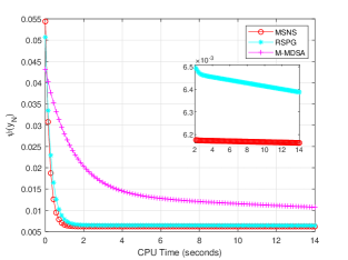
(a) $NS=10000$, $n=500$, $\epsilon=0.1$

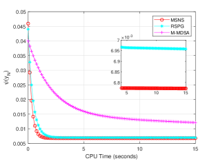
(b) $NS=20000$, $n=500$, $\epsilon=0.1$

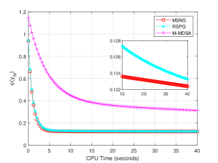
(c) $NS=10000$, $n=1000$, $\epsilon=0.1$

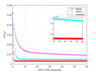
(d) $NS=20000$, $n=1000$, $\epsilon=0.1$

Figure 1: Average objective values corresponding to the training data v.s. CPU time of 20 runs for different values of sample size $NS$, dimension $n$, when $\epsilon=0.1$.

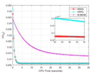
(a) $NS=10000$, $n=500$, $\epsilon=0.05$

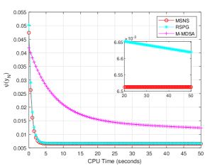
(b) $NS=20000$, $n=500$, $\epsilon=0.05$

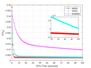
(c) $NS=10000$, $n=1000$, $\epsilon=0.05$

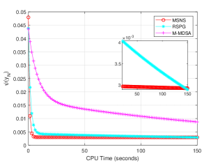
(d) $NS=20000$, $n=1000$, $\epsilon=0.05$

Figure 2: Average objective values corresponding to the training data v.s. CPU time of 20 runs for different values of sample size $NS$, dimension $n$, when $\epsilon=0.05$.

To see stability, we show in Tables 2 and 3 the mean (Mean) and the variance (Var), over 20 runs, of the objective values (Obj) corresponding to the testing data at the computed solution $\widehat{x}$ by a certain method. The Obj is the empirical mean of the stochastic objective value $F(\widehat{x},\xi)+H(\widehat{x},\xi)$. The empirical mean is taken over a large testing data consisting of data samples $K=50000$ as done in Nemirovski . From Tables 2 and 3, the average objective values corresponding to the testing data, the average accuracy, and the average CPU time of the MSNS method are significantly better than that of the other methods in almost all cases. Moreover, the MSNS method provides the results of the objective values with small variance.

Table 2: The mean and variance of the objective values, the average accuracy and CPU time when $\epsilon=0.1$ of 20 runs

$n$	$NS$	ALG.	Obj	Obj	Acc	CPU
			Mean	Var	(Avg.)	(Avg.)
500	10000	MSNS	0.3071	2.90e-06	0.9817	44.2968
		RSPG	0.3093	3.92e-06	0.9815	386.0023
		M-MDSA	0.3402	5.01e-05	0.9785	55.4375
		2-RSPG	0.3092	2.05e-06	0.9815	334.7219
		2-RSPG-V	0.3089	3.35e-06	0.9815	336.8773
	20000	MSNS	0.3001	6.95e-07	0.9818	45.4281
		RSPG	0.3031	7.95e-07	0.9813	386.8484
		M-MDSA	0.3357	2.00e-05	0.9783	57.9516
		2-RSPG	0.3028	1.05e-03	0.9814	424.7093
		2-RSPG-V	0.3027	9.57e-07	0.9816	437.3919
1000	10000	MSNS	0.1715	1.64e-06	0.9978	102.5140
		RSPG	0.1741	1.61e-06	0.9975	1335.9727
		M-MDSA	0.2351	1.21e-04	0.9924	103.5156
		2-RSPG	0.1741	1.71e-06	0.9976	1669.5687
		2-RSPG-V	0.1739	1.51e-06	0.9976	1705.7171
	20000	MSNS	0.1603	3.19e-07	0.9979	105.4656
		RSPG	0.1646	6.66e-06	0.9976	1687.0039
		M-MDSA	0.2293	2.71e-05	0.9924	105.9687
		2-RSPG	0.1644	7.01e-07	0.9977	1768.0484
		2-RSPG-V	0.1643	7.78e-07	0.9977	1824.6265

Table 3: The mean and variance of the objective values, the average accuracy and CPU time when $\epsilon=0.05$ of 20 runs

$n$	$NS$	ALG.	Obj	Obj	Acc	CPU
			Mean	Var	(Avg.)	(Avg.)
500	10000	MSNS	0.3061	1.71e-06	0.9813	266.1671
		RSPG	0.3076	1.85e-06	0.9811	1951.5351
		M-MDSA	0.3411	4.76e-05	0.9781	391.4593
		2-RSPG	0.3074	1.61e-06	0.9812	1848.8625
		2-RSPG-V	0.3072	1.88e-06	0.9812	1835.7265
	20000	MSNS	0.2995	1.47e-06	0.9823	273.3210
		RSPG	0.3008	1.68e-06	0.9820	2693.3601
		M-MDSA	0.3324	1.91e-05	0.9791	399.0406
		2-RSPG	0.3008	1.36e-06	0.9821	1915.3305
		2-RSPG-V	0.3007	1.63e-06	0.9821	2462.5796
1000	10000	MSNS	0.1704	1.42e-06	0.9977	514.4062
		RSPG	0.1721	1.48e-06	0.9975	10347.2710
		M-MDSA	0.2364	5.96e-05	0.9923	529.8718
		2-RSPG	0.1719	1.95e-06	0.9976	8604.6609
		2-RSPG-V	0.1717	1.78e-06	0.9976	9281.1523
	20000	MSNS	0.1595	4.61e-07	0.9979	534.6511
		RSPG	0.1614	6.66e-07	0.9978	7236.1585
		M-MDSA	0.2283	3.21e-05	0.9924	541.6226
		2-RSPG	0.1616	6.88e-07	0.9978	9701.7789
		2-RSPG-V	0.1614	5.32e-07	0.9978	9028.8843

4.2 Real datasets

We do numerical experiments on four real datasets described below for our experiments.

$\bullet$ Wisconsin breast cancer dataset from the UCI repository (699 patterns) can be downloaded from the web. Features are computed from a digitized image of a fine needle aspirate (FNA) of a breast mass. They describe characteristics of the cell nuclei present in the image.

$\bullet$ Statlog (Australian Credit Approval) dataset also comes from the UCI repository, downloaded from the web. This file concerns credit card applications. All attribute names and values have been changed to meaningless symbols to protect confidentiality of the data. This dataset is interesting because there is a good mix of attributes – continuous, nominal with small numbers of values, and nominal with larger numbers of values.

$\bullet$ Credit Approval dataset also comes from the UCI repository. This file concerns credit card applications. All attribute names and values have been changed to meaningless symbols to protect confidentiality of the data. This dataset is interesting because there is a good mix of attributes, continuous, nominal with small numbers of values, and nominal with larger numbers of values.

$\bullet$ Ecoli dataset is also refer to the protein localization sites dataset, downloaded from the web. The dataset describes the problem of classifying Ecoli proteins using their amino acid sequences in their cell localization sites. That is, predicting how a protein will bind to a cell based on the chemical composition of the protein before it is folded. We analyzed Ecoli dataset in its 2-class versions, i.e., Ecoli(B). Ecoli(B) from the first 4 proteins and the remaining ones. The details of the described datasets are resumed in Table 4.

Table 4: Details of the datasets

Dataset	Classes	Sample size	Dimension
Wisconsin breast cancer	2	699	10
Statlog	2	690	14
Credit Approval	2	690	15
Ecoli(B)	2	366	343

We choose the optimal values of $\lambda_{1}$ and $t$ via 3-fold cross-validation (CV) using 20 random runs, which are determined by varying them on the grid $\{10^{-2},10^{-1},2^{-2},2^{-1},1\}$ and the values with the best average accuracy are chosen for each of the MSNS, RSPG, M-MDSA, 2-RSPG, and 2-RSPG-V methods. For real datasets, we also compare with the classical SVM model chang for which the cost parameter $c$ and parameter $g$ in kernel function were determined by varying them on the grid $\{10^{-4},10^{-2},10^{-1},1,10\}$ recommended by Melacci on page 1168.

We find that the average CPU time is related to the parameters $\lambda_{1}$ and $t$ for each of the MSNS, RSPG, M-MDSA, 2-RSPG, and 2-RSPG-V methods. More specifically, the CPU time decreases as $\lambda_{1}$ decreases, and also decreases as $t$ decreases for each of the above method. We take the MSNS method as an example to illustrate the reason for this phenomenon. When $\lambda_{1}$ is fixed, along with the decreasing of $t$, $D=t/2$ decreases and consequently the maximum iteration number $N$ decreases according to (52). The batch size $m$ also decreases with $N$ by (49). Similarly, when $t$ is fixed, $L_{f}$ decreases with $\lambda_{1}$, resulting in a decrease in the maximum number of iterations $N$ by (52). The batch size $m$ also decreases with $N$ by (49). We record the average CPU time of the MSNS method, along with different $\lambda_{1}$ and $t$ for two datasets: Wisconsin breast cancer and Ecoli(B) as examples in Tables 5 and 6, respectively. The relationship of the CPU time and the values of parameters $\lambda_{1}$ and $t$ can be seen clearly from the two tables.

Table 5: CPU time of the MSNS method corresponding to different values of $\lambda_{1}$, $t$, on the dataset – Wisconsin breast cancer

$t\backslash\lambda_{1}$	$10^{-2}$	$10^{-1}$	$2^{-2}$	$2^{-1}$	1
$10^{-2}$	0.0074	0.0038	0.0040	0.0043	0.0060
$10^{-1}$	0.0246	0.0259	0.0310	0.0366	0.0453
$2^{-2}$	0.0653	0.0661	0.0784	0.0942	0.1231
$2^{-1}$	0.1258	0.1433	0.1631	0.2079	0.2725
1	0.2676	0.3013	0.3574	0.4541	0.6094

Table 6: CPU time of the MSNS method corresponding to different values of $\lambda_{1}$, $t$, on the dataset – Ecoli(B)

$t\backslash\lambda_{1}$	$10^{-2}$	$10^{-1}$	$2^{-2}$	$2^{-1}$	1
$10^{-2}$	0.3350	0.3659	0.3885	0.4317	0.5288
$10^{-1}$	9.8397	10.2583	10.9856	12.2976	15.0089
$2^{-2}$	39.5078	41.1832	44.0774	48.2053	58.5466
$2^{-1}$	103.0333	114.9313	127.1659	134.4300	163.9350
1	211.7660	285.0719	322.8352	399.9200	471.5500

We record in Table 7 the average optimal values of parameters $(t,\lambda_{1})$ or $(c,g)$, together with the corresponding average accuracy and the average CPU time in seconds. We can see that our MSNS method has the best average accuracy in all the datasets. The CPU time of the MSNS method is not the shortest, but it is only a little bit longer than the shortest one and hence is acceptable.

Table 7: Accuracy, the values of $(t,\lambda_{1})$ or $(c,g)$ and CPU time determined by 3-fold CV

Dataset	ALG.	$t$	$\lambda_{1}$	$c$	$g$	Acc	CPU
Wisconsin breast cancer	MSNS	$10^{-1}$	$10^{-2}$	-	-	0.9686	0.0097
	RSPG	$10^{-1}$	$10^{-1}$	-	-	0.9664	0.0597
	M-MDSA	$10^{-1}$	$10^{-2}$	-	-	0.9617	0.0111
	2-RSPG	$10^{-1}$	$10^{-2}$	-	-	0.9672	0.0674
	2-RSPG-V	$10^{-1}$	$10^{-2}$	-	-	0.9678	0.0566
	SVM	-	-	10	$10^{-2}$	0.9614	0.0046
Statlog	MSNS	$2^{-2}$	$10^{-2}$	-	-	0.8670	0.0163
	RSPG	$2^{-2}$	$10^{-2}$	-	-	0.8631	0.0487
	M-MDSA	1	$10^{-1}$	-	-	0.8569	0.1602
	2-RSPG	$2^{-2}$	$10^{-2}$	-	-	0.8654	0.0765
	2-RSPG-V	$2^{-2}$	$10^{-2}$	-	-	0.8656	0.0580
	SVM	-	-	10	$10^{-4}$	0.8609	0.0254
Credit Approval	MSNS	$2^{-1}$	1	-	-	0.8595	0.2636
	RSPG	$2^{-2}$	1	-	-	0.8589	0.4914
	M-MDSA	1	$2^{-1}$	-	-	0.8562	0.4694
	2-RSPG	1	1	-	-	0.8591	2.9523
	2-RSPG-V	$2^{-2}$	1	-	-	0.8590	0.5832
	SVM	-	-	1	$10^{-2}$	0.8591	0.0155
Ecoli(B)	MSNS	$10^{-2}$	$10^{-1}$	-	-	0.8720	0.3659
	RSPG	$10^{-2}$	$2^{-1}$	-	-	0.8501	0.2826
	M-MDSA	$10^{-1}$	$10^{-1}$	-	-	0.8423	10.2845
	2-RSPG	1	$10^{-2}$	-	-	0.8540	160.8485
	2-RSPG-V	1	$10^{-2}$	-	-	0.8542	169.9453
	SVM	-	-	10	$10^{-4}$	0.7107	0.0767

5 Concluding remarks

In this paper, we propose a mini-batch stochastic Nesterov’s smoothing (MSNS) method for solving a class of constrained convex nonsmooth composite optimization problems with noisy zero-order and first-order information. We show the convergence of the MSNS method, together with its optimal iteration complexity. Numerical experiments on a support vector machine (SVM) model using both synthetic datasets and real datasets, demonstrate the effectiveness and efficiency of the proposed MSNS method, compared with several state-of-the-art methods.

References

• (1) Nesterov, Y.: Smooth minimization of non-smooth functions. Math. Program. 103(1), 127-152 (2005).
• (2) Robbins, H., Monro, S.: A stochastic approximation method. Ann. Math. Statist. 22(3), 400-407 (1951).
• (3) Polyak, B.: New stochastic approximation type procedures. Automat. i Telemekh. 7(2), 98-107 (1990). (English translation: Automation and Remote Control).
• (4) Polyak, B., Juditsky, A.: Acceleration of stochastic approximation by averaging. SIAM J. Control Optim. 30(4), 838-855 (2006).
• (5) Nemirovski, A., Juditsky, A., Lan, G., Shapiro, A.: Robust stochastic approximation approach to stochastic programming. SIAM J. Optim. 19(4), 1574-1609 (2009).
• (6) Nemirovsky, A., Yudin, D. B.: Problem Complexity and Method Efficiency in Optimization. Wiley, New York (1983).
• (7) Kleywegt, A., Shapiro, A., Homem-de-Mello, T.: The sample average approximation method for stochastic discrete optimization. SIAM J. Optim. 12(2), 479-502 (2002).
• (8) Shapiro, A.: Monte Carlo sampling methods. Handbooks in Oper. Res. Manag. Sci. 10, 353-425 (2003).
• (9) Lan, G., Nemirovski, A., Shapiro, A.: Validation analysis of mirror descent stochastic approximation method. Math. Program. 134(2), 425-458 (2012).
• (10) Nemirovski, A., Juditsky, A., Lan, G., Shapiro, A.: Robust stochastic approximation approach to stochastic programming. SIAM J. Optim. 19(4), 1574-1609 (2009).
• (11) Ghadimi, S., Lan, G., Zhang, H.: Mini-batch stochastic approximation methods for nonconvex stochastic composite optimization. Math. Program. 155(1-2), 267-305 (2016).
• (12) Wang, X., Wang, X., Yuan, Y.-X.: Stochastic proximal quasi-Newton methods for non-convex composite optimization. Optim. Methods Softw. 34(5), 922-948 (2019).
• (13) Chen, S., Ma, S., So, A. M.-C., Zhang, T.: Proximal gradient method for nonsmooth optimization over the Stiefel manifold. SIAM J. Optim. 30(1), 210-239 (2020).
• (14) Xiao, X.: A unified convergence analysis of stochastic Bregman proximal gradient and extragradient method. J. Optim. Theory Appl. 188(3), 605-627 (2021).
• (15) Zhang, C., Chen, X.: Smoothing projected gradient method and its application to stochastic linear complementarity problem. SIAM J. Optim. 20(2), 627-649 (2009).
• (16) Chen, X.: Smoothing methods for nonsmooth, nonconvex minimization. Math. Program. Ser. B, 134, 71-99 (2012).
• (17) Bian, W., Chen, X.: Linearly constrained non-Lipschitz optimization for image restoration. SIAM J. Imaging Sci. 8(4), 2294-2322 (2015).
• (18) Liu, Y.-F., Ma, S., Dai, Y.-H., Zhang, S.: A smoothing SQP framework for a class of composite $L_{q}$ minimization over polyhedron. Math. Program. Ser. A, 158(1-2), 467-790 (2016).
• (19) Zhang, C., Chen, X.: A smoothing active set method forl inearly constrained non-Lipschitz nonconvex optimization. SIAM J. Optim. 30(1), 1-30 (2020).
• (20) Sion, M.: On general minimax theorems. Pac. J. Math. 8(1), 171-176 (1957).
• (21) Beck, A.: First-Order Methods in Optimization. SIAM, Philadelphia (2017).
• (22) Noble, W. S.: What is a support vector machine? Nat. Biotechnol. 24(12), 1565-1567 (2006).
• (23) Huang, S., Cai, N., Pacheco, P. P., Narrandes, S., Wang, Y., Xu, W.: Applications of support vector machine (SVM) learning in cancer genomics. Cancer Genom. Proteom. 15(1), 41-51 (2018).
• (24) Rodriguez, R., Vogt, M., Bajorath, J.: Support vector machine classification and regression prioritize different structural features for binary compound activity and potency value prediction. ACS Omega. 2(10), 6371-6379 (2017).
• (25) Shivaswamy, P. K., Jebara, T.: Relative Margin Machines. NIPS. 19, 1481-1488 (2008).
• (26) Melacci, S., Belkin, M.: Laplacian support vector machines trained in the primal. J. Mach. Learn. Res. 12(3), 1149-1184 (2011).
• (27) Chang, C., Lin, C.: LIBSVM: a library for support vector machines. ACM T. Intel. Syst. Tec. 2(3), 1-27 (2011).