Dynamics, symmetries, anomaly and vortices in a rotating cosmic string background

Abstract

Non-relativistic conformally invariant systems in a rotating cosmic string (conical) spacetime are analyzed at the classical and quantum levels by means of the gravitoelectromagnetic interpretation of the background. Solutions of the equations of motion are found by employing a local canonical transformation, that leads to their natural interpretation in terms of Riemann surfaces. The cone parameter $\alpha$ and the angular velocity $\Omega$ of the background determine the existence of hidden symmetries. Globally defined higher order integrals associated with perihelion of geodesic orbits appear at rational values of $\alpha$. For the harmonic oscillator system with frequency $\omega$, the integrals responsible for the trajectory closure arise only for rational values of $\alpha$ and $|\gamma|=|\Omega/\omega|$, with $|\gamma|=1$ corresponding to the Landau problem. We face a quantum anomaly problem since the hidden symmetry operators can only be constructed when $\alpha$ is integer. Such operators are non-local in the case of the free particle. For the harmonic oscillator, the symmetry generators are obtained with the help of the conformal bridge transformation. We also study a multi-particle version of the harmonic oscillator system with $|\gamma|=1$ using the mean-field theory and find that the emerging vortex structure respects a singular point of the background.

1 Introduction

In physics, a quantum anomaly occurs when classical symmetries fail at the quantum level. The well known examples of this are the so-called Adler-Bell-Jackiw anomaly in electrodynamics [1, 2], where the conservation of axial vector current is violated in quantum theory, and the gauge anomalies, where quantum corrections do not preserve classical gauge invariance. [3]. In this article, we face a type of quantum anomaly similar to what was observed in [4], which is more related to the structure of the spacetime background than quantum corrections, and where the conserved operators commute with the Hamiltonian, but their action can produce non-physical eigenstates.

The phenomenon of a quantum anomaly produced by geometric constraints is not too strange since it is natural to expect that spacetime has to influence on the dynamics of the systems that live on it. The very well known examples where the geometry effects essentially on the symmetry properties of the particle systems are provided by the integrable dynamics of a test particle in the Kerr black hole due to the Carter integral [5], and the enhanced supersymmetry that characterizes the motion of a spinning particle in a Kerr-Newman black hole [6]. In these two cases we are dealing with hidden symmetries and the so-called Killing and Killing-Yano tensors associated with them [7, 8, 9, 10, 11, 12]. Other effects related with geometry are the Lense-Thirring effect produced by gravitoelectromagnetic fields [13, 14] and the production of additional particles in quantum field theories in curved spaces [15, 16].

The specific issue of the “geometrical quantum anomaly” that we refer above was observed by us earlier when we analyzed the problem of canonical quantization of non-relativistic dynamics in the cosmic string spacetime [17], which is characterized by a geometrical parameter $\alpha$ that encodes the information on the conical singularity of the background [18, 19, 20, 21]. Various authors explored this topic in the past [22, 23, 24, 25, 26], but their research avoids going deeper into quantum symmetries, since they claim that there are difficulties in defining self-adjoint operators correctly. In our case, we were able to construct the well defined hidden symmetry generators and gave a non-linear algebraic description of conformally invariant quantum systems [27] living in this spacetime only for natural values of $\alpha$. This goes in contrast with the classical level (and for this reason we have a quantum anomaly), where the well defined on phase space hidden integrals of motion can be constructed for any rational value of $\alpha$.

In our study, the so-called conformal bridge transformation [28, 29] played a crucial role. This relatively new technique relates asymptotically free conformally invariant models with their harmonically confined versions. Therefore, if one system has an anomaly issue, then the other also faces this problem [17]. On the other hand, the (super)conformally invariant systems are the simplest integrable models that can be studied in different geometric backgrounds, and which are essential with their own right due to appearance in various applications in physics. For some recent interesting results see [30, 31, 32, 33] and references therein.

One may expect that a way to cure the geometric anomaly in our case should again be related to geometry. With this in mind, we address here the idea to include a homogeneous rotation of angular velocity $\Omega$ about the cone’s symmetry axis in the corresponding spacetime metric as a possible solution to the anomaly issue. As is well known, such a rotation induces gravitoelectromagnetic fields [13, 14]. Historically, the importance of studying rotating reference frames comes from the simple fact that the Earth’s rotation strongly influences the experiments carried out on it. In quantum case, the rotation results, in particular, in appearance of the Sagnac effect [34], the impossibility of forming rigid flows [35], and modifications in the Hall effect [36, 37]. Since rotation also introduces a kind of singularity at the point in which its axis intersects the two-dimensional surface, it is somewhat natural to expect that its inclusion, at least, should provide some new insight in the context of the quantum anomaly problem. In addition, by switching on of a rotationally-invariant harmonic trap with its independent frequency parameter, one could also hope to dynamically solve the anomaly problem.

Although the formulated idea has not worked as it was expected, we have obtained several interesting results that apply to both single-particle and many-particle systems in conical backgrounds, and this article aims to report them.

Let us describe the organization of the article and briefly summarize the results. Sec. 2 investigates the geodesic motion in a homogeneously rotating conical background, which we interpret as a cosmic string with a gravitoelectromagnetic field. We describe there a particular type of an integral of motion which plays a role similar to that of the Laplace-Runge-Lentz vector in the Kepler problem [11, 38]. At the classical level, this quantity is a well defined phase space function for arbitrary values of $\Omega$ but only when $\alpha$ is rational. It has a well defined non-local quantum analog only for integer values of $\alpha$. In Sec. 3, we supply the system with a harmonic trap potential with frequency $\omega$ and study its classical dynamics. As a result, we obtain an analog of the Euclidean exotic rotationally invariant harmonic oscillator (ERIHO) system [39], but now in the cosmic string background. This system has closed orbits and integrals of motion associated with a hidden symmetry only when both parameters $|\gamma|=|\Omega/\omega|$ and $\alpha$ take rational values. In particular case $|\gamma|=1$, the system is equivalent to the Landau problem in a space with a topological defect [40, 41]. In Sec. 4, we consider the quantum version of the system using the conformal bridge transformation [28, 29]. There we show that the quantum analogs of the hidden symmetry generators are well defined operators that correctly reflect the degeneracy of energy levels only when $\alpha$ takes integer values. In Sec. 5, we consider the mean-field theory approximation to study the Bose-Einstein condensation of the harmonically trapped systems in a conical vessel in their Landau problem phases corresponding to $\gamma=\pm 1$. Similar problem for the Euclidean case was considered in [42, 43]. As a result, we show that the appearing vortex structure respects a singular point of the rotating cosmic string background. In Sec. 6, the discussion of the obtained results and outlook are presented. In Appendix A we show how the nontrivial integrals found in Sec. 2 can be obtained from the non-relativistic two-dimensional free particle in the inertial reference frame ($\Omega=0$).

2 Dynamics in rigidly rotating spacetimes

The weak field approximation of general relativity is characterized by appearance of electric- and magnetic-like fields. They are usually called the gravitoelectric and gravitomagnetic fields because their action on massive test particles is similar to the action of external electric and magnetic fields on charged particles. An indirect verification of gravitoelectromagnetism is provided by relativistic jets [44, 45] appearing in the study of rotating black holes, and in the observed excess of energy and luminosity produced by quasars and active galactic nuclei, which are explained by the Lense-Thirring effect [13, 14]. Recently, gravitomagnetism has also been used to explain the rotation curves of galaxies as an alternative to dark matter [46].

The dynamics of test particles in rigidly rotating spacetime backgrounds is essentially affected by the appearance of gravitoelectromagnetic fields at the classical and quantum levels. For special values of the parameters of such and similar systems, classical dynamics of test particles can be completely integrable due to appearance of hidden symmetries, which also reveal themselves in peculiar properties of the corresponding quantum systems [5, 6, 10, 11, 12, 17, 39]. This section aims to investigate such effects for geodesic motion in a rotating conical background.

2.1 Classical picture

The simplest case in which gravitoelectromagnetic effects can be observed corresponds to a $(3+1)$-dimensional Minkowski vacuum subjected to a uniform rotation. The metric of this spacetime with the angular velocity $\Omega$ oriented along the $z$ axis is given by

$$ds^{2}=-c^{2}dt^{2}+(d\rho^{2}+\rho^{2}(d\varphi+\Omega dt)^{2}+dz^{2})\,.$$ (2.1)

Lagrangian of a non-relativistic test particle that experiences geodesic motion in this background is obtained from the relativistic action

$$-mc\int\sqrt{-ds^{2}}=-mc^{2}\bigintsss\sqrt{1-\frac{1}{c^{2}}\left(\left(\frac{d\rho}{dt}\right)^{2}+\rho^{2}\left(\frac{d\varphi}{dt}+\Omega\right)^{2}+\left(\frac{dz}{dt}\right)^{2}\right)}\,\,dt$$ (2.2)

by taking the limit $c\rightarrow\infty$. It is given by

$$L=L_{\Omega}+\frac{m}{2}\dot{z}^{2}\,,\qquad L_{\Omega}=\frac{m}{2}(\dot{\rho}^{2}+\rho^{2}(\dot{\varphi}+\Omega)^{2})\,,$$ (2.3)

where the dot denotes time derivative. This is a Lagrangian of a free particle in a rotating reference frame in cylindrical coordinates. It can be obtained in an alternative way from the non-relativistic free particle system in inertial reference frame by means of a time dependent canonical transformation, see Appendix A. Written in Cartesian coordinates $x^{1}=\rho\cos\varphi$ and $x^{2}=\rho\sin\varphi$, Lagrangian $L_{\Omega}$ takes the form

$$L_{\Omega}=\frac{m}{2}\dot{x}^{i}\dot{x}^{i}+\frac{m}{2}\Omega^{2}x^{i}x^{i}+\frac{q_{{}_{GM}}}{c}\dot{x}^{i}A^{i}\,,\qquad A^{i}=\frac{\Omega c}{2}\epsilon^{ij}x^{j}\,.$$ (2.4)

Here, $A^{i}$ can be interpreted as a two-dimensional vector potential of a gravitomagnetic field applied to a particle with gravitomagnetic charge $q_{{}_{GM}}=-2m$. As a result, two-dimensional Lagrangian (2.4) corresponds to that of the Landau problem in symmetric gauge with magnetic field $B_{G}=\epsilon_{ij}\partial_{i}A_{j}=-\Omega c$, supplemented with an isotropic quadratic centrifugal potential $-\frac{1}{2}m\Omega^{2}x^{i}x^{i}$. The latter can be reinterpreted as the external gravitoelectric potential applied to a particle with gravitoelectric charge $q_{{}_{GE}}=-m$ . The canonical Hamiltonian for the system (2.4) is

$$H_{\Omega}=\frac{1}{2m}p_{i}p_{i}-\Omega p_{\varphi}\,,\qquad p_{\varphi}=x_{1}p_{2}-x_{2}p_{1}\,.$$ (2.5)

The peculiarity of the system (2.4) is that the additional repulsive centrifugal potential term exactly balances the confining effect of the magnetic field as is seen from the solution of the classical equations of motion,

$$x_{+}(t)=x_{1}+ix_{2}=\rho e^{i\varphi}=e^{-i\Omega t}\left(Bt+C\right)\,,$$ (2.6)

where $B$ and $C$ are complex constants of the dimensions of $\dot{x}$ and $x$, respectively, and the bracket term corresponds to a free dynamics of a particle in a plane.

A conical singularity can be introduced by reducing metric (2.1) to a conical surface $z(\rho)=\rho\cot{\beta}$, that results in the (2+1)-dimensional spacetime with a metric

$$ds^{2}=-c^{2}dt^{2}+\alpha^{2}d\rho^{2}+\rho^{2}(d\varphi+\alpha\Omega dt)^{2}\,,$$ (2.7)

$$0<\rho<\infty\,,\qquad 0\leq\varphi\leq 2\pi\,,\qquad\alpha^{2}=1+\cot^{2}{\beta}>1\,.$$ (2.8)

To simplify future calculations, we have rescaled $\Omega\rightarrow\alpha\Omega$. When $\Omega=0$, this metric can be associated with a $(2+1)$-dimensional cosmic string spacetime with the identification $\alpha=(1-4\mu c^{-2}G)^{-1}$, where $G$ is the Newton constant and $\mu$ is the linear mass density of the string [17]. If we allow the parameter $\alpha$ to take values in the interval $(0,\,1)$, metric (2.7) can be associated, on the one hand, with a geometric background describing radial dislocations in superfluids [14], and, on the other hand, with metric of an anti-gravitating cosmic string with negative mass density (which corresponds to a wormhole’s background) [14, 48].

Note here that in the case of $\Omega\not=0$, $\alpha>1$ one can consider metric (2.7), (2.8) as that corresponding to a rotating conical vessel of an infinitesimal thickness. This interpretation will be employed in Section 5.

In the spacetime (2.7), the non-relativistic geodesic Lagrangian is given by

$$L^{(\alpha)}_{\Omega}=\frac{m}{2}\left(\alpha^{2}\dot{\rho}^{2}+\rho^{2}(\dot{\varphi}+\alpha\Omega)^{2}\right)\,.$$ (2.9)

It is obtained in the same way as for the flat case by substituting $ds^{2}$ in (2.2) for the metric (2.7), (2.8) . In terms of the conical metric in Cartesian coordinates,

$$g_{ij}=\delta_{ij}+(\alpha^{2}-1)\frac{1}{(x^{1})^{2}+(x^{2})^{2}}\left(\begin{array}[]{cc}(x^{1})^{2}&x^{1}x^{2}\\ x^{1}x^{2}&(x^{2})^{2}\end{array}\right)\,,$$ (2.12)

Lagrangian (2.9) takes the form

$$L_{\Omega}^{(\alpha)}=\frac{m}{2}g_{ij}\dot{x}^{i}\dot{x}^{j}+\frac{m}{2}\Omega^{2}g_{ij}x^{i}x^{j}+\frac{q_{{}_{GM}}}{c}g_{ij}\dot{x}^{i}A^{(\alpha)j}\,,\qquad A^{(\alpha)i}=\frac{\alpha\Omega c}{2}(x^{2},-x^{1})\,.$$ (2.13)

For $\alpha>1$, $A^{(\alpha)i}$ can be interpreted as a vector potential corresponding to the Landau problem in the symmetric gauge with magnetic field $B^{(\alpha)}=-\alpha B_{G}=\alpha\Omega c$, which is perpendicular to the surface of the cone.

Classical Hamiltonian of the system (2.9) is

$$H_{\Omega}^{(\alpha)}=\frac{1}{2m}\left(\frac{1}{\alpha^{2}}p_{\rho}^{2}+\frac{1}{\rho^{2}}p_{\varphi}^{2}\right)-\alpha\Omega p_{\varphi}\,,$$ (2.14)

from where one sees that the repulsive quadratic potential appearing in (2.13) again compensates the confinement effect of the magnetic field. It is clear that the system is rotationally invariant, $p_{\varphi}=const$, and so, has the integral of motion

$$H_{0}^{(\alpha)}=\frac{1}{2m}\left(\frac{1}{\alpha^{2}}p_{\rho}^{2}+\frac{1}{\rho^{2}}p_{\varphi}^{2}\right).$$ (2.15)

The latter is the Hamiltonian of a free particle in a conical geometry in the inertial reference frame.

In the case of arbitrary values of the parameter $\alpha$, there are also formal dynamical integrals of motion 

$$P_{\pm}^{(\alpha)}=e^{\pm i\alpha\Omega t}\Pi_{\pm}^{(\alpha)}\,,\qquad G_{\pm}^{(\alpha)}=me^{\pm i\alpha\Omega t}\,\Xi_{\pm}^{(\alpha)}\,,$$ (2.16)

where

$$\Pi_{\pm}^{(\alpha)}=\left(\frac{p_{\rho}}{\alpha}\pm i\frac{p_{\varphi}}{\rho}\right)e^{\pm i\frac{\varphi}{\alpha}}\,,\qquad\Xi_{\pm}^{(\alpha)}=\alpha\rho e^{\pm i\frac{\varphi}{\alpha}}-\frac{t}{m}\Pi_{\pm}^{(\alpha)}$$ (2.17)

are the analogues of the canonical momenta and the Galilean boost generators in the conical geometry [17]. They are globally well defined phase space functions in the flat case $\alpha=1$, see Appendix A, as well as for integer values of $\alpha$ greater than one. Integrals (2.16) generate the two-dimensional Heisenberg algebra, $\{G_{\pm}^{(\alpha)},P_{\mp}^{(\alpha)}\}=2m$, $\{G_{\pm}^{(\alpha)},P_{\pm}^{(\alpha)}\}=0$, $\{G_{+}^{(\alpha)},G_{-}^{(\alpha)}\}=\{P_{+}^{(\alpha)},P_{-}^{(\alpha)}\}=0$. From them, one can construct the well defined in the phase space, rotationally invariant generators of dilatations, $D^{(\alpha)}$, and special conformal transformations, $K^{(\alpha)}$,

$$D^{(\alpha)}=\frac{1}{4m}(G_{+}^{(\alpha)}P_{-}^{(\alpha)}+G_{-}^{(\alpha)}P_{+}^{(\alpha)})=\frac{1}{2}\rho p_{\rho}-H^{(\alpha)}_{0}t\,,$$ (2.18)

$$K^{(\alpha)}=\frac{1}{2m}G_{+}^{(\alpha)}G_{-}^{(\alpha)}=\frac{1}{2}m\alpha^{2}\rho^{2}-2D^{(\alpha)}t-H^{(\alpha)}_{0}t^{2}\,.$$ (2.19)

Quadratic in $P_{\pm}^{(\alpha)}$ and $G_{\pm}^{(\alpha)}$ dynamical integrals $D^{(\alpha)}$ and $K^{(\alpha)}$ together with the Hamiltonian $H_{\Omega}^{(\alpha)}=\frac{1}{2m}P_{+}^{(\alpha)}P_{-}^{(\alpha)}-\alpha\Omega p_{\varphi}$ satisfy the centrally extended $\mathfrak{sl}(2,\mathbb{R})$ conformal algebra

$$\{D^{(\alpha)},H^{(\alpha)}_{\Omega}\}=H^{(\alpha)}_{\Omega}+Z^{(\alpha)}\,,\quad\{D^{(\alpha)},K^{(\alpha)}\}=-K^{(\alpha)}\,,\quad\{K^{(\alpha)},H^{(\alpha)}_{\Omega}\}=2D^{(\alpha)}\,,\quad$$ (2.20)

in which $Z^{(\alpha)}=\alpha\Omega p_{\varphi}=i\frac{\Omega}{2m}(G_{+}^{(\alpha)}P_{-}^{(\alpha)}-G_{-}^{(\alpha)}P_{+}^{(\alpha)})$ plays a role of the central charge. The Casimir of this algebra is

$$\mathcal{C}=(D^{(\alpha)})^{2}-(H_{\Omega}^{(\alpha)}+Z^{(\alpha)})K^{(\alpha)}+\frac{1}{4\Omega^{2}}(Z^{(\alpha)})^{2}=0\,.$$ (2.21)

The central extension here is rather formal since the central charge can be absorbed by changing the generator $H^{(\alpha)}_{\Omega}$ for $H^{(\alpha)}_{0}=H^{(\alpha)}_{\Omega}+Z^{(\alpha)}=\frac{1}{2m}P_{+}^{(\alpha)}P_{-}^{(\alpha)}$, that transforms (2.20) into $\mathfrak{gl}(2,\mathbb{R})\cong\mathfrak{sl}(2,\mathbb{R})\oplus\mathfrak{u}(1)$ algebra, where $\mathfrak{sl}(2,\mathbb{R})$ is the usual conformal algebra generated by $H^{(\alpha)}_{0}$, $D^{(\alpha)}$ and $K^{(\alpha)}$, and $\mathfrak{u}(1)$ is generated by $p_{\varphi}$. The value of the $\mathfrak{sl}(2,\mathbb{R})$ Casimir $C=(D^{(\alpha)})^{2}-H_{0}^{(\alpha)}K^{(\alpha)}$ reduces in this case to $-\frac{\alpha^{2}}{4}p_{\varphi}^{2}$.

From the dynamical integral (2.19) and Casimir (2.21) one gets that $\rho^{2}$ as a function of time is given by the quadratic polynomial

$$\rho^{2}(t)=a(t-t_{*})^{2}+b^{2}$$ (2.22)

with $a=2H^{(\alpha)}_{0}/(m\alpha^{2})$, $b^{2}=p_{\varphi}^{2}/(2mH^{(\alpha)}_{0})$ and

$$t_{*}=-D^{(\alpha)}/H^{(\alpha)}_{0}\,.$$ (2.23)

One finds that at the moment of time $t=t_{*}$, the variable $\rho$ takes the minimum value,

$$\rho(t_{*})=b=(2mH_{0}^{(\alpha)})^{-\frac{1}{2}}|p_{\varphi}|:=\rho_{*}\,,$$ (2.24)

that corresponds to the ‘perihelion’ of the trajectory.

To find the angle evolution and identify the trajectories of the particle, we consider the transformation

$$\rho\rightarrow\alpha\rho\,,\qquad\varphi\rightarrow\alpha^{-1}\varphi\,.$$ (2.25)

Under this rescaling of the variables, Lagrangian (2.9) is transformed into $L_{\Omega}$ in (2.4), and therefore, locally the geodesic motion in metric (2.7) is given by $x_{+}(t)=x^{1}(t)+ix^{2}(t)=\rho(t)e^{i\varphi(t)}$, where now

$$\rho(t)=\alpha^{-1}|Bt+C|\,,\qquad e^{i\varphi(t)}=e^{-i\alpha\Omega t}|Bt+C|^{-\alpha}(Bt+C)^{\alpha}\,,$$ (2.26)

and so,

$$x_{+}(t)=\alpha^{-1}|w|^{1-\alpha}(w(t))^{\alpha}\,,\qquad w(t)=e^{-i\Omega t}(Bt+C)\,.$$ (2.27)

Parametrizing complex integration constants as $B=Ve^{i\vartheta_{1}}$ and $C=Re^{i\vartheta_{2}}$, and employing the corresponding Hamiltonian equations of motion of the system, one finds that the integral $H_{0}^{(\alpha)}$, the angular momentum $p_{\varphi}$, the perihelion of the orbit $\rho_{*}$ and the corresponding moment of time $t_{*}$ reduce to

$$H_{0}^{(\alpha)}=\frac{m}{2}V^{2}\,,\qquad p_{\varphi}=\alpha^{-1}mVR\sin(\vartheta_{1}-\vartheta_{2})\,,$$ (2.28)

$$\rho_{*}=\alpha^{-1}R|\sin(\vartheta_{1}-\vartheta_{2})|\,,\qquad t_{*}=-RV^{-1}\cos(\vartheta_{1}-\vartheta_{2})\,,$$ (2.29)

while the total mechanical energy is expressed as $H_{\Omega}^{(\alpha)}=\frac{m}{2}V^{2}(1-2\Omega RV^{-1}\sin(\vartheta_{1}-\vartheta_{2}))\,.$ From these relations it follows that when the constants of integration are chosen so that $\vartheta_{1}-\vartheta_{2}=\pi n$, $n\in\mathbb{Z}$, the angular momentum is zero, and with $V\neq 0$ the particle falls to the origin of the coordinate system being the vertex of the cone. One also notes that when the mechanical energy $H_{\Omega}^{(\alpha)}$ takes positive (negative) values, the translational (rotational) motion governed by $H^{(\alpha)}_{0}$ ($-\alpha\Omega p_{\varphi}$) dominates. Furthermore, when $V=0$, we have $H^{(\alpha)}_{0}=0$, and the orbit is a circle of radius $\rho_{*}$.

The second equation in (2.26) can be written in an equivalent form

$$e^{i\alpha^{-1}(\varphi-\varphi_{*})}=e^{-i\Omega(t-t_{*})}\left[\frac{1}{\rho_{*}\rho}\left(\rho_{*}^{2}+i\frac{p_{\varphi}}{m\alpha}(t-t_{*})\right)\right]\,,$$ (2.30)

where $\varphi_{*}=\varphi(t_{*})$. After replacing here the time evolution parameter by its expression in terms of the phase space functions,

$$t-t_{*}=\frac{\rho p_{\rho}}{2H_{0}^{(\alpha)}}\,,$$ (2.31)

that is directly obtained from (2.23) and the definition of $D^{(\alpha)}$, and multiplying (2.30) by $\mp(2mH_{0}^{(\alpha)})^{1/2}e^{-i\alpha^{-1}\varphi}$, we get as a result the following complex pair $I_{\pm}^{(\alpha)}$ of the true (not depending explicitly on time) mutually conjugate integrals of motion,

$$I_{\pm}^{(\alpha)}=\exp(\pm i\frac{\Omega\rho p_{\rho}}{2H_{0}^{(\alpha)}})\,\Pi_{\pm}^{(\alpha)}\,,\qquad$$ (2.32)

see Eq. (2.17) and Appendix A. In the case of $\alpha=1$ and $\Omega=0$ these integrals reduce to the complex linear combinations $p_{\pm}=p_{1}\pm ip_{2}$ of the momentum vector components of the free particle in $\mathbb{R}^{2}$ . Obviously the quantities $f(H_{0}^{(\alpha)},p_{\varphi})I_{\pm}^{(\alpha)}$ also are integrals of motion for arbitrary choice of the function $f(\xi,\eta)$.

The integrals $I_{+}^{(\alpha)}$ and $I_{-}^{(\alpha)}$ have the Poisson brackets $\{I_{+}^{(\alpha)},I_{-}^{(\alpha)}\}=2im\alpha\Omega\,,$ and so, are similar to the complex linear combinations of the integrals corresponding to a center of a circular orbit in the Landau problem in a plane. However, due to the phase factor, these integrals are globally well defined functions in the phase space only in the cases of $\alpha=1/k$ with $k=1,2,\ldots$. For general case of rational values $\alpha=q/k$ with $q=1,2,\ldots,$ the integrals

$$(I_{\pm}^{(q/k)})^{q}=\exp(\pm i\frac{q\Omega\rho p_{\rho}}{2H_{0}^{(q/k)}})(\Pi_{\pm}^{(q/k)})^{q}$$ (2.33)

can be considered instead of (2.32) since they do not have the phase problem. Here and in what follows we assume that the fraction $q/k$ is irreducible, i.e., $q$ and $k$ are mutually prime.

Another way to obtain the formal integrals (2.32) is by starting from the integrals of the system in the reference frame at rest ($\Omega=0$), and applying to them the canonical transformation

$$\exp(\lambda F^{(\alpha)})\star f=f+\sum_{n=1}^{\infty}\frac{\lambda^{n}}{n!}\{F^{(\alpha)},\{\ldots,\{F^{(\alpha)},f\underbrace{\}\ldots\}\}}_{n}:=T_{F^{(\alpha)}}(\lambda)\star(f)\,,\quad$$ (2.34)

$$F^{(\alpha)}=\alpha\frac{\rho p_{\rho}p_{\varphi}}{2H_{0}^{(\alpha)}}\,,\qquad\lambda=-\Omega\,.$$ (2.35)

The chosen generator $F^{(\alpha)}$ of the canonical transformation includes dependence on the dilatation dynamical integral $D^{(\alpha)}$ taken at $t=0$, see Eq. (2.18), and so, is not an integral of motion. By means of the Poisson brackets relations

$$\{F^{(\alpha)},H_{0}^{(\alpha)}\}=\alpha p_{\varphi}\,,\qquad\{F^{(\alpha)},p_{\varphi}\}=0\,,$$ (2.36)

$$\{F^{(\alpha)},\frac{1}{2}\rho p_{\rho}\}=F^{(\alpha)}\,,\qquad\{\frac{1}{2}\rho p_{\rho},\Pi_{\pm}^{(\alpha)}\}=\frac{1}{2}\Pi_{\pm}^{(\alpha)}\,,\qquad\{p_{\varphi},\Pi_{\pm}^{(\alpha)}\}=\mp i\Pi_{\pm}^{(\alpha)}\,,$$ (2.37)

one gets as a result

$$T_{F^{(\alpha)}}(-\Omega)\star(H_{0}^{(\alpha)})=H_{\Omega}^{(\alpha)}\,,\qquad T_{F^{(\alpha)}}(-\Omega)\star((H_{0}^{(\alpha)})^{-\frac{1}{2}}\Pi_{\pm}^{(\alpha)})=(H_{0}^{(\alpha)})^{-\frac{1}{2}}I_{\pm}^{(\alpha)}\,,$$ (2.38)

from were it is deduced

$$T_{F^{(\alpha)}}(-\Omega)\star\left(((H_{0}^{(\alpha)}+\alpha\Omega p_{\varphi})^{2})^{1/4}(H_{0}^{(\alpha)})^{-\frac{1}{2}}\Pi_{\pm}^{(\alpha)}\right)=I_{\pm}^{(\alpha)}\,.$$ (2.39)

In the case $\alpha=q/k$ we get $T_{F^{(q/k)}}(-\Omega)\star((H_{0}^{(q/k)})^{-\frac{q}{2}}(\Pi_{\pm}^{(q/k)})^{q})=(H_{0}^{(q/k)})^{-\frac{q}{2}}(I_{\pm}^{(q/k)})^{q}\,.$ This technique will be useful for the quantum analysis in the next section.

To complete the classical analysis, we visualise the trajectories of the particle for different values of $\alpha$. To draw them in the $(x^{1},x^{2})$ plane, where $x^{1}$ and $x^{2}$ are real and imaginary parts of $x_{+}$ in (2.27), it is necessary to take into account some properties associated with the function $f_{\alpha}(w)=w^{\alpha}$ in the $w$ complex plane. First, the function $f_{\alpha}(w)$ is analytic in the $w$ complex plane when $\alpha$ is an integer number, and then there are no problems to draw the orbit. On the other hand, when $\alpha=q/k$ with $q,k=1,2,\ldots$, $f_{q/k}(w)$ is a $k$-valued function, and its entire domain corresponds to a Riemann surface with $k$ sheets. In this case, for $k>1$ we have to take care on which sheet we are in a definite moment of time. Finally, $f_{\alpha}(w)$ with irrational $\alpha$ is an infinite-valued function, whose domain corresponds to a Riemann surface with infinite number of sheets. In Fig. 1 some examples of trajectories are presented by following the indicated peculiarities.

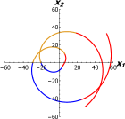
(a) $\alpha=1/3$, $\dot{\varphi}_{*}<0$.

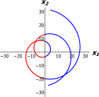
(b) $\alpha=1/2$, $\dot{\varphi}_{*}<0$.

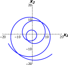
(c) $\alpha=1$, $\dot{\varphi}_{*}<0$.

(d) $\alpha=4/3$, $\dot{\varphi}_{*}<0$.

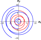
(e) $\alpha=3/2$, $\dot{\varphi}_{*}<0$.

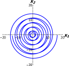
(f) $\alpha=2$, $\dot{\varphi}_{*}<0$.

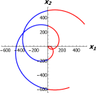
(g) $\alpha=1/2$, $\dot{\varphi}_{*}>0$.

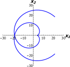
(h) $\alpha=1$, $\dot{\varphi}_{*}=0$.

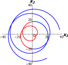
(i) $\alpha=3/2$, $\dot{\varphi}_{*}>0$.

Figure 1: Trajectories for different rational values of the cone parameter $\alpha$ and $\Omega>0$. The colour change in the trajectories indicates the transition from one Riemann surface sheet to another. In figures 1(a) and 1(d) (1(b), 1(e), 1(g) and 1(i)) the corresponding Riemann surface has three (two) sheets, while in figures 1(c) and 1(f) the Riemann surface is the complex plane itself. For $\dot{\varphi}_{*}=\dot{\varphi}(t_{*})=\alpha(V(R\sin(\vartheta_{1}-\vartheta_{2}))^{-1}-\Omega)>0$, the external angular velocity $\Omega>0$ is subtracted from the intrinsic angular velocity of the particle at the position of “perihelion” of the orbit, producing a small loop that does not enclose the origin. For $\dot{\varphi}_{*}<0$, such small loops are not generated. When $\dot{\varphi}_{*}=0$, a cusp appears (figure 1(h)).

2.2 Quantum picture

After quantization we get the Hamiltonian operator

$$\hat{H}_{\Omega}^{(\alpha)}=\hat{H}_{0}^{(\alpha)}-\alpha\Omega\hat{p}_{\varphi}\,,$$ (2.40)

which represents a linear combination of the free particle Hamiltonian in a conical background [17] and the quantum angular momentum operator,

$$\hat{H}_{0}^{(\alpha)}=-\frac{\hbar^{2}}{2m}\left(\frac{1}{\alpha^{2}\rho}\frac{\partial}{\partial\rho}\left(\rho\frac{\partial}{\partial\rho}\right)+\frac{1}{\rho^{2}}\frac{\partial^{2}}{\partial\varphi^{2}}\right)\,,\qquad\hat{p}_{\varphi}=-i\hbar\frac{\partial}{\partial\varphi}\,.$$ (2.41)

The eigenstates that simultaneously diagonalize these two operators, and therefore are the eigenstates of the system (2.40), are given by the functions

$$\psi_{\kappa,\ell}^{(\alpha)}(r,\varphi)=\sqrt{\frac{\kappa}{2\pi\alpha}}J_{\alpha|\ell|}(\kappa r)e^{i\ell\varphi}\,,$$ (2.42)

where $J_{\beta}(\eta)$ are the Bessel functions of the first kind. These states satisfy the eigenvalue equations

$$\hat{H}_{0}^{(\alpha)}\psi_{\kappa,\ell}^{(\alpha)}(r,\varphi)=\frac{\hbar^{2}\kappa^{2}}{2m\alpha^{2}}\psi_{\kappa,\ell}^{(\alpha)}(r,\varphi)\,,\qquad\hat{p}_{\varphi}\psi_{\kappa,\ell}^{(\alpha)}(r,\varphi)=\hbar\ell\psi_{\kappa,\ell}^{(\alpha)}(r,\varphi)\,,$$ (2.43)

$$\hat{H}_{\Omega}^{(\alpha)}\psi_{\kappa,\ell}^{(\alpha)}=E_{\kappa,\ell}^{(\alpha)}\psi_{\kappa,\ell}^{(\alpha)}\,,\qquad E_{\kappa,\ell}^{(\alpha)}=\frac{\hbar^{2}\kappa^{2}}{2m\alpha^{2}}-\alpha\Omega\hbar\ell\,,\quad\kappa>0\,,\quad\ell=0,\pm 1,\ldots\,,$$ (2.44)

as well as the orthogonality relation $\innerproduct{\psi_{\kappa,\ell}^{(\alpha)}}{\psi_{\kappa^{\prime},\ell^{\prime}}^{(\alpha)}}=\ \delta_{\ell,\ell^{\prime}}\delta(\kappa-\kappa^{\prime})$, where

$$\innerproduct{\Psi_{1}}{\Psi_{2}}=\iint\Psi_{1}^{*}\Psi_{2}\sqrt{g}\,dx^{1}dx^{2}=\alpha\int_{0}^{\infty}rdr\int_{0}^{2\pi}d\varphi\Psi_{1}^{*}\Psi_{2}\,$$ (2.45)

is the inner product in conical geometry, $g=\det\,(g_{ij})$. The formal eigenfunctions corresponding to $\kappa=0$ and $\ell\not=0$, which are given by $r^{\alpha|\ell|}e^{i\ell\varphi}$ and $r^{-\alpha|\ell|}e^{i\ell\varphi}$, are excluded from the physical sets of eigenstates since they are not Dirac delta normalizable with respect to the scalar product (2.45). The physical eigenstates with zero energy correspond to all those functions whose quantum numbers satisfy the condition $\hbar\kappa^{2}=2m\alpha^{3}\Omega\ell$, as well as the constant function when $\kappa=\ell=0$. The latter does not belong to the set (2.42), but can be obtained by a limiting procedure

$$\lim_{\kappa\rightarrow 0}\sqrt{\frac{2\pi\alpha}{\kappa}}\psi_{\kappa,0}^{(\alpha)}=1\,.$$ (2.46)

For the sake of definiteness in what follows we assume $\Omega>0$.

It is notable that unlike the energy eigenvalues, the form of the eigenfunctions $\psi_{\kappa,\ell}^{(\alpha)}(r,\varphi)$ is independent of the value of the external angular velocity $\Omega$. Therefore, if for certain values of $\alpha$, the system has well defined integral operators related to a degeneration of the spectrum, they should modify coherently both indices (discrete and continuous) in a corresponding wave function. In this way from the condition $E_{\kappa,\ell}^{(\alpha)}=E_{\tilde{\kappa},\ell\pm 1}^{(\alpha)}$ we obtain

$$\tilde{\kappa}=\kappa_{\pm}=\kappa\sqrt{1\pm\frac{2m\alpha^{3}\Omega}{\hbar\kappa^{2}}}\,.$$ (2.47)

This relation implies that when $\hbar\kappa^{2}<2m\alpha^{3}\Omega$, $\kappa_{-}$ becomes an imaginary number, and therefore, physical integral operators that produce the transformation $\psi_{\kappa,\ell}^{(\alpha)}\rightarrow\psi_{\kappa_{-},\ell-1}^{(\alpha)}$ must annihilate all physical eigenstates with $\hbar\kappa^{2}\leq 2m\alpha^{3}\Omega$. No restrictions appear for the eigenvalue $\ell$ here.

In order to try to construct such symmetry integral operators, we introduce the operators

$$\hat{W}_{-}^{(\alpha)}=e^{-i\frac{\Omega}{\hbar}\hat{F}}\,,\qquad\hat{W}_{+}^{(\alpha)}=(\hat{W}_{-}^{(\alpha)})^{-1}=e^{i\frac{\Omega}{\hbar}\hat{F}}\,.$$ (2.48)

The quantum version $\hat{F}$ of the classical quantity (2.35) we fix so that the commutation relations

$$[\hat{F}^{(\alpha)},\hat{H}_{0}^{(\alpha)}]=i\hbar\alpha\hat{p}_{\varphi}\,,\quad[\hat{F}^{(\alpha)},\hat{p}_{\varphi}]=0\,$$ (2.49)

will be satisfied in correspondence with (2.36). This implies the relations

$$[\hat{H}_{0}^{(\alpha)},\hat{W}_{\pm}^{(\alpha)}]=\pm\Omega\alpha\hat{p}_{\varphi}W_{\pm}^{(\alpha)}\,,\qquad[\hat{p}_{\varphi},\hat{W}_{\pm}^{(\alpha)}]=0\,.$$ (2.50)

The appearance of the quantity $(H_{0}^{(\alpha)})^{-1}$ in the classical definition of $F$ means that some non-trivial quantization prescription must be employed to escape a singularity in the corresponding quantum operators. By taking the symmetric ordering ,

$$\hat{F}^{(\alpha)}=\frac{\alpha}{4}\left[\hat{p}_{\varphi}\left((\hat{H}_{0}^{(\alpha)})^{-1}\hat{D}_{0}^{(\alpha)}+\hat{D}_{0}^{(\alpha)}(\hat{H}_{0}^{(\alpha)})^{-1}\right)+\left((\hat{H}_{0}^{(\alpha)})^{-1}\hat{D}_{0}^{(\alpha)}+\hat{D}_{0}^{(\alpha)}(\hat{H}_{0}^{(\alpha)})^{-1}\right)\hat{p}_{\varphi}\right]\,,\quad$$ (2.51)

we produce the Hermitian operator, $\hat{F}^{(\alpha)}=\hat{F}^{(\alpha)}{}^{\dagger}$, where $\hat{D}_{0}^{(\alpha)}=\frac{-i\hbar}{2}(\rho\frac{\partial}{\partial\rho}+1)$ coincides with the dilatation operator taken at $t=0$. In this construction $\hat{W}_{\pm}^{(\alpha)}$ formally are unitary and their action is well defined on eigenstates of the form (2.42). However, the action of the operator (2.51) on the constant wave function is not defined. As this last eigenstate corresponds to a free particle at rest in the inertial reference frame, with zero eigenvalue of $\hat{H}_{0}^{(\alpha)}$ and zero angular momentum, it seems reasonable to treat it separately for the moment. With these considerations, operator (2.51) is simplified,

$$\hat{F}^{(\alpha)}=\frac{\alpha}{2}(\hat{H}_{0}^{(\alpha)})^{-1}(2\hat{D}_{0}^{(\alpha)}-i\hbar)\hat{p}_{\varphi}\,.$$ (2.52)

Then, the unitary operator $\hat{W}_{+}^{(\alpha)}$ and its inverse, $\hat{W}_{-}^{(\alpha)}=\hat{W}_{+}^{(\alpha)}{}^{\dagger}$, can be employed to produce the following unitary transformation,

$$\hat{W}_{-}^{(\alpha)}\hat{H}_{0}^{(\alpha)}\hat{W}_{+}^{(\alpha)}=\hat{H}_{\Omega}^{(\alpha)}\,,\qquad\hat{W}_{-}^{(\alpha)}\hat{p}_{\varphi}\hat{W}_{+}^{(\alpha)}=\hat{p}_{\varphi}\,,$$ (2.53)

and as a consequence, the transformed eigenstates $\Psi_{\kappa,\ell}^{(\alpha)}=\hat{W}_{-}^{(\alpha)}\psi_{\kappa,\ell}^{(\alpha)}$ should satisfy

$$\hat{H}_{0}^{(\alpha)}\Psi_{\kappa,\ell}^{(\alpha)}=\left(\frac{\hbar^{2}\kappa^{2}}{2m\alpha^{2}}+\hbar\alpha\Omega\ell\right)\Psi_{\kappa,\ell}^{(\alpha)}\,,\qquad\hat{p}_{\varphi}\Psi_{\kappa,\ell}^{(\alpha)}=\hbar\ell\Psi_{\kappa,\ell}^{(\alpha)}\,,\qquad\hat{H}_{\Omega}^{(\alpha)}\Psi_{\kappa,\ell}^{(\alpha)}=\frac{\hbar^{2}\kappa^{2}}{2m\alpha^{2}}\Psi_{\kappa,\ell}^{(\alpha)}\,.\qquad$$ (2.54)

From these expressions we conclude that the transformed states have to be of the form

$$\Psi_{\kappa,\ell}^{(\alpha)}\sim\psi_{\kappa_{\ell},\ell}^{(\alpha)}\,,\qquad\kappa_{\ell}=\kappa\sqrt{1+\frac{2m\alpha^{3}\Omega\ell}{\hbar\kappa^{2}}}\,.$$ (2.55)

However, in this way non-physical eigenstates can be obtained for negative values of $\ell$ for $\Omega>0$. For this reason we continue using states (2.42) instead of (2.55). To construct the symmetry operators associated with degeneracy of energy eigenvalues, we apply the similarity transformation to the integral operators of the free particle in a conical geometry in the reference frame at rest, $\Omega=0$. It is known from the previous work [17] that such symmetry operators exist only when $\alpha=q$ (otherwise, they can produce non-physical eigenstates), and are given by

$$(\hat{\Pi}_{\pm}^{(q)})^{q}\,,\qquad\text{where}\qquad\hat{\Pi}_{\pm}^{(q)}=-i\hbar e^{\pm i\frac{\varphi}{q}}\left(\frac{1}{q}\frac{\partial}{\partial\rho}\pm i\frac{1}{\rho}\frac{\partial}{\partial\varphi}\right)\,.$$ (2.56)

After applying the unitary transformation to them one gets the mutually Hermitian conjugate operators

$$(\hat{I}_{+}^{(q)})^{q}=\hat{W}_{-}^{(q)}(\hat{\Pi}_{+}^{(q)})^{q}\hat{W}_{+}^{(q)}\,,\qquad(\hat{I}_{-}^{(q)})^{q}=((\hat{I}_{+}^{(q)})^{q})^{\dagger}\,.$$ (2.57)

These operators commute with the Hamiltonian $\hat{H}_{\Omega}^{(\alpha)}$ and can be applied to all physical states of the form (2.42). Their action can be deduced by means of the commutation relations

$$[\hat{H}_{0}^{(q)},(\hat{I}_{\pm}^{(q)})^{q}]=\pm q\Omega\hbar(\hat{I}_{\pm}^{(q)})^{q}\,,\qquad[\hat{p}_{\varphi},(\hat{I}_{\pm}^{(q)})^{q}]=\pm\hbar(\hat{I}_{\pm}^{(q)})^{q}\,,$$ (2.58)

from which one obtains

$$(\hat{I}_{\pm}^{(q)})^{q}\psi_{\kappa,\ell}^{(\alpha)}\sim\psi_{\kappa_{\pm},\ell\pm 1}^{(\alpha)}\,,$$ (2.59)

where $\kappa_{\pm}$ correspond to (2.47). The operators $(\hat{I}_{\pm}^{(q)})^{q}$ produce exactly the necessary change of the index in the wave functions which does not change the corresponding energy eigenvalue. Nevertheless, in the cases when $\kappa$ satisfies the condition $\hbar\kappa^{2}<2mq^{3}\Omega$, the operator $(\hat{I}_{-}^{(q)})^{q}$ produces non-physical eigenstates. To avoid this problem, we can take the regularized operators

$$\hat{\mathscr{I}}_{-}=(\hat{I}_{-}^{(q)})^{q}\Theta\left(\frac{1}{\hbar\Omega}\hat{H}_{0}^{(q)}-q\right)\,,\quad\hat{\mathscr{I}}_{+}=\Theta\left(\frac{1}{\hbar\Omega}\hat{H}_{0}^{(q)}-q\right)(\hat{I}_{+}^{(q)})^{q}\,,$$ (2.60)

where $\Theta(\eta)$ is the Heaviside step function. When $\hat{\mathscr{I}}_{-}$ acts on the eigenstates, the Heaviside function annihilates all those physical eigenstates, which can potentiality be transformed into non-physical states by the action of $(\hat{I}_{-}^{(q)})^{q}$. On the other hand, $(\hat{I}_{+}^{(q)})^{q}$ cannot produce non-physical states, and if $\hbar\kappa^{2}<2mq^{3}\Omega$, then $\hbar\kappa_{+}^{2}=\hbar\kappa^{2}+2mq^{3}\Omega\geq 2mq^{3}\Omega$. As a consequence, the action of the operator $\Theta\left(\frac{1}{\hbar\Omega}\hat{H}_{0}^{(q)}-q\right)$ after the application of $(\hat{I}_{+}^{(q)})^{q}$ reduces to multiplication by one. The action of the symmetry operators (2.60) is well defined on all energy eigenstates including the constant wave function corresponding to zero eigenvalue of the operator $\hat{H}^{(\alpha)}_{0}$.

In conclusion of this section we note that as classically the system reveals a hidden symmetry in the case of rational values of the conical background parameter $\alpha$, while at the quantum level we are able to identify the hidden symmetry described by non-local operators in the case of only integer values of $\alpha$, we face a kind of a quantum anomaly here.

A rather natural question is if the anomaly related to the geometry of the system can be “cured” by a dynamic extension of the system. We investigate such a kind of extension of the system in the next section.

3 Classical ERIHO system in a conical space

Recently, in [39] we considered the exotic rotationally invariant harmonic oscillator generated from the planar free particle system by application of the conformal bridge transformation [28, 29]. The model is described by the Hamiltonian 

$$H_{\gamma}=\frac{1}{2m}p_{i}p_{i}+\frac{1}{2}m\omega^{2}x_{i}x_{i}+\gamma\omega\epsilon_{ij}x_{i}p_{j}=\frac{1}{2m}\left(p_{\rho}^{2}+\rho^{-2}p_{\varphi}^{2}\right)+\frac{1}{2}m\omega^{2}\rho^{2}+\gamma\omega p_{\varphi}\,,$$ (3.1)

and its peculiar properties were studied by us from the perspective of symmetries. The solutions of the equations of motion of the system correspond to closed trajectories only when $\gamma$ is a rational number. This property is reflected in the existence of the additional integrals of motion in the case $\gamma\in\mathbb{Q}$, which define the orientation of the orbit like the Laplace-Runge-Lenz vector in Kepler’s problem. At the quantum level, these additional integrals explain the degeneracy of the spectrum of the model that only appears when $\gamma$ takes rational values. In spite of the explicit rotational invariance of (3.1), the classical and quantum properties of the model resemble those of the planar anisotropic Euclidean and Minkowskian harmonic oscillator systems. This is not accidental since both systems turn out to be related by a non-trivial unitary $\mathfrak{so}(2)$-non-invariant transform composed from the special $\mathfrak{su}(2)$ rotation considered by us earlier in [17] and supplemented by an additional Bogolyubov transformation.

After changing $\omega\rightarrow\Omega=-\gamma\omega$, one finds that the Lagrangian of the system (3.1) can be presented in the form

$$L_{\gamma}=L_{\Omega}-\frac{1}{2}m(\gamma^{-1}\Omega)^{2}x^{i}x^{i}=\frac{m}{2}\dot{x}^{i}\dot{x}^{i}-\frac{m}{2}(\gamma^{-2}-1)\Omega^{2}x^{i}x^{i}+\frac{q_{GM}}{c}\dot{x}^{i}A^{i}\,,$$ (3.2)

where $L_{\Omega}$ is given by Eq. (2.4). As a consequence, the model (3.1) admits two other physical interpretations [39]. First, it corresponds to a two-dimensional isotropic harmonic oscillator in a non-inertial reference frame rotating with angular velocity $\Omega$. Alternatively, it can be considered as the Landau problem in the presence of an additional external harmonic potential $V_{\gamma}=\frac{m}{2}(\gamma^{-2}-1)\Omega^{2}x^{i}x^{i}$. When $\gamma^{2}<1$ ($\gamma^{2}>1$), the sign of this quadratic potential is positive (negative), so it produces an attractive (repulsive) harmonic force on the particle. The intermediate case $\gamma^{2}=1$ corresponds to the two Landau phases of the system different in two possible orientations of the magnetic field orthogonal to the plane, which are defined by the sign of $\gamma$.

In this section we explore the direct classical and quantum generalization of the ERIHO system to a conical spacetime. As we will see, in this case one has to take into account both parameters $\gamma$ and $\alpha$ to find closed trajectories with which the integrals of motion of the hidden symmetry are associated. Before the detailed analysis, one would expect that the presence of an additional parameter $\gamma$, which is associated here with an additional “gravitoelectric” harmonic potential, could “cure” the quantum anomaly related with the background geometry, that was described in the previous section. In particular case of $\gamma^{2}=1$, this also will allow us to investigate the Landau problem in conical background from the perspective of dynamics and symmetries.

3.1 Classical picture

To find the analogue of the ERIHO system in a conical background, we start by changing the implicit flat metric tensor $\delta_{ij}$ in Lagrangian (3.2) by the conical metric tensor (2.12), that yields

$$L_{\gamma}^{(\alpha)}=L_{\Omega}^{(\alpha)}-\frac{1}{2}m\gamma^{-2}\Omega^{2}g_{ij}x^{i}x^{j}=\frac{m}{2}g_{ij}\dot{x}^{i}\dot{x}^{j}-\frac{m}{2}(\gamma^{-2}-1)\Omega^{2}g_{ij}x^{i}x^{j}+\frac{q_{GM}}{c}g_{ij}\dot{x}^{i}A^{(\alpha)j}\,,$$ (3.3)

where $L_{\Omega}^{(\alpha)}$ and $A^{(\alpha)i}$ are given by (2.13). This Lagrangian means that, again, the system can be interpreted as an isotropic harmonic oscillator in a conical background of a cosmic string in a non-inertial uniformly rotating reference frame. Alternatively, we can consider system (3.3) as the Landau problem in conical geometry, extended by an external quadratic potential $V_{\gamma}^{(\alpha)}=\frac{m}{2}(\gamma^{-2}-1)\Omega^{2}g_{ij}x^{i}x^{j}=\frac{m}{2}(\gamma^{-2}-1)\Omega^{2}\alpha^{2}\rho^{2}$. From the nature of this additional potential term it is clear that one has to distinguish the cases $\gamma^{2}<1$ and $\gamma^{2}>1$, where this potential is attractive and repulsive, and the Landau phases at $\gamma=\pm 1$. The case $\gamma=\infty$ corresponds here to the system considered in the previous section. After performing the Legendre transformation and by identifying $\Omega=-\gamma\omega$, one gets the Hamiltonian of the system, which takes more simple form in polar coordinates,

$$H_{\gamma}^{(\alpha)}=\frac{1}{2m}\left(\alpha^{-2}p_{\rho}^{2}+\rho^{-2}p_{\varphi}^{2}\right)+\frac{1}{2}m\omega^{2}\alpha^{2}\rho^{2}+\gamma\omega\alpha p_{\varphi}\,.$$ (3.4)

We assume without loss of generality that $\omega>0$. Comparing (3.4) with the Hamiltonian of the Euclidean planar ERIHO system (3.1) [39], it is obvious that the former can be obtained from the latter by means of the local canonical transformation

$$\rho\rightarrow\alpha\rho\,,\qquad p_{\rho}\rightarrow\alpha^{-1}p_{\rho}\,,\qquad\varphi\rightarrow\alpha^{-1}\varphi\,,\qquad p_{\varphi}\rightarrow\alpha p_{\varphi}\,.$$ (3.5)

So, (3.4) is the ERIHO system in a conical background.

In terms of Cartesian coordinates, canonical transformation (3.5) is

$$x_{1}\rightarrow X_{\alpha,1}=\alpha\rho\cos(\frac{\varphi}{\alpha})\,,\qquad x_{2}\rightarrow X_{\alpha,2}=\alpha\rho\sin(\frac{\varphi}{\alpha})\,,$$ (3.6)

$$p_{1}\rightarrow P_{\alpha,1}=\frac{p_{\rho}}{\alpha}\cos(\frac{\varphi}{\alpha})-\frac{p_{\varphi}}{\rho}\sin(\frac{\varphi}{\alpha})\,,\qquad p_{2}\rightarrow P_{\alpha,2}=\frac{p_{\rho}}{\alpha}\sin(\frac{\varphi}{\alpha})+\frac{p_{\varphi}}{\rho}\cos(\frac{\varphi}{\alpha})\,,$$ (3.7)

$$\{X_{\alpha,i},X_{\alpha,j}\}=\{P_{\alpha,i},P_{\alpha,j}\}=0\,,\qquad\{X_{\alpha,i},P_{\alpha,j}\}=\delta_{ij}\,,$$ (3.8)

while the conical metric $ds^{2}=g_{ij}dx^{i}dx^{j}$ takes the form $ds^{2}=dX_{\alpha,1}^{2}+dX_{\alpha,2}^{2}$ . In local canonical variables ($X_{\alpha,i}$, $P_{\alpha,i}$) Hamiltonian (3.4) has the form of the ERIHO Hamiltonian in usual Cartesian coordinates,

$$H_{\gamma}^{(\alpha)}=\frac{1}{2m}(P_{\alpha,1}^{2}+P_{\alpha,2}^{2})+\frac{m\omega^{2}}{2}(X_{\alpha,1}^{2}+X_{\alpha,2}^{2})+\omega\gamma\epsilon_{ij}X_{i,\alpha}P_{j,\alpha}\,.$$ (3.9)

To analyse the dynamics and symmetries of the system, it is convenient to pass over to the following complex combinations of the local canonical variables,

$$b_{\alpha,1}^{-}=\frac{1}{\sqrt{2}}(a_{\alpha,1}^{-}-ia_{\alpha,2}^{-})=\frac{1}{2}e^{-i\frac{\varphi}{\alpha}}\left(\alpha\sqrt{m\omega}\rho+\frac{p_{\varphi}}{\sqrt{m\omega}\rho}+\frac{ip_{\rho}}{\alpha\sqrt{m\omega}}\right)\,,\quad b_{\alpha,1}^{+}=(b_{\alpha,1}^{-})^{*}\,,$$ (3.10)

$$b_{\alpha,2}^{-}=\frac{1}{\sqrt{2}}(a_{\alpha,1}^{-}+ia_{\alpha,2}^{-})=\frac{1}{2}e^{i\frac{\varphi}{\alpha}}\left(\alpha\sqrt{m\omega}\rho-\frac{p_{\varphi}}{\sqrt{m\omega}\rho}+\frac{ip_{\rho}}{\alpha\sqrt{m\omega}}\right)\,,\quad b_{\alpha,2}^{+}=(b_{\alpha,2}^{-})^{*}\,,$$ (3.11)

$$a_{\alpha,i}^{\pm}=\sqrt{\frac{m\omega}{2}}\left(\,X_{\alpha,i}\mp\frac{i}{m\omega}\,P_{\alpha,i}\right)\,.$$ (3.12)

They satisfy the Poisson bracket relations $\{b_{\alpha,j}^{-},b_{\alpha,k}^{-}\}=\{b_{\alpha,j}^{+},b_{\alpha,k}^{+}\}=0$, $\{b_{\alpha,j}^{-},b_{\alpha,k}^{+}\}=-i\delta_{jk}$, and reduce the Hamiltonian to the form like that of the anisotropic harmonic oscillator,

$$H_{\gamma}^{(\alpha)}=\omega\left(\ell_{1}b_{\alpha,1}^{+}b_{\alpha,1}^{-}+\ell_{2}b_{\alpha,2}^{+}b_{\alpha,2}^{-}\right)\,,\qquad\ell_{1}=1+\gamma\,,\qquad\ell_{2}=1-\gamma\,.$$ (3.13)

However, here the angular momentum is

$$p_{\varphi}=\alpha^{-1}(b_{\alpha,1}^{+}b_{\alpha,1}^{-}-b_{\alpha,2}^{+}b_{\alpha,2}^{-})\,,$$ (3.14)

and Hamiltonian (3.13) is rotationally invariant, $\{p_{\varphi},H_{\gamma}^{(\alpha)}\}=0$.

The equations of motion can easily be solved in variables $b_{\alpha,i}^{\pm}$,

$$\dot{b}_{\alpha,i}^{\pm}=\{b_{\alpha,i}^{\pm},H_{\gamma}^{(\alpha)}\}=\pm i\omega\ell_{i}b_{\alpha,i}^{\pm}\quad\Rightarrow\quad b_{\alpha,i}^{\pm}(t)=e^{\pm i\omega\ell_{i}t}b_{\alpha,i}^{\pm}(0):=b_{\alpha,i}^{\pm}\,.$$ (3.15)

Using the relation $\sqrt{m\omega}(X_{\alpha,1}+iX_{\alpha,2})=b^{+}_{\alpha,1}+b^{-}_{\alpha,2}$, one gets

$$X_{\alpha,+}(t)=X_{\alpha,1}(t)+iX_{\alpha,2}(t)=R_{1}e^{i\vartheta_{1}}e^{i\omega\ell_{1}t}+R_{2}e^{-i\vartheta_{2}}e^{-i\omega\ell_{2}t}\,,$$ (3.16)

where $R_{1,2}\geq 0$, $R^{2}_{1}+R_{2}^{2}>0$, and $\vartheta_{1,2}\in\mathbb{R}$ are the constants of integration, $b_{\alpha,i}^{\pm}(0)=R_{i}e^{\pm i\vartheta_{i}}/\sqrt{m\omega}$. From here one sees that $X_{\alpha,+}(t)$ is a periodic in time $t$ function only when $(1+\gamma)/(1-\gamma)\in\mathbb{Q}$, that implies rational values for the parameter $\gamma$. This, however, does not mean periodicity of the conical trajectories as $X_{\alpha,i}$ are not globally well defined functions of polar coordinates for general values of the parameter $\alpha$ : $X_{\alpha,i}(\rho,\varphi=0)\neq X_{\alpha,i}(\rho,\varphi=2\pi)$ for $\alpha\neq 1/n$, $n=2,3,\ldots$. To find the evolution of the polar coordinates $\rho(t)$ and $\varphi(t)$, we use the relations

$$\rho^{2}(t)=\frac{1}{\alpha^{2}}|X_{\alpha,+}(t)|^{2}\,,\qquad e^{i\alpha^{-1}\varphi(t)}=\left(\frac{X_{\alpha,+}(t)}{\alpha\rho(t)}\right)\,\Rightarrow\,e^{i\varphi(t)}=\left(\frac{X_{\alpha,+}(t)}{\alpha\rho(t)}\right)^{\alpha}\,,$$ (3.17)

$$x_{+}(t)=x_{1}(t)+ix_{2}(t)=\rho(t)e^{i\varphi(t)}=\frac{1}{\alpha}|X_{\alpha,+}(t)|^{1-\alpha}(X_{\alpha,+}(t))^{\alpha}\,.$$ (3.18)

Similar to the free rotation case from the previous section, in order to visualize the trajectory, we should be careful with the complex function $f_{\alpha}=(X_{\alpha,+}(t))^{\alpha}$ in dependence on the value of $\alpha$. The $X_{q/k,+}(t)$ describes a curve that encircles the origin of coordinates in the plane $(X_{\alpha,1},X_{\alpha,2})$ when $\gamma^{2}\neq 1$. The only exception is possible in the Landau case $\gamma^{2}=1$ for certain selection of the initial data, that we discuss below. However, in general case these curves are closed only when $\gamma$ takes rational values. Then, for $\alpha=q/k$, complex function $f_{q/k}$ is $k$-valued, whose domain is a Riemann surface of $k$ sheets, and we have to pay attention to the transitions from one sheet to another while we draw the trajectory. When $k=1$, the Riemann surface is the complex plane itself. For irrational $\alpha$, function $f_{\alpha}$ is infinite-valued, and the path is not closed.

The closure of a trajectory implies the appearance of additional integrals of motion corresponding to hidden symmetries. From the structure of the Hamiltonian we distinguish the two obvious conserved quantities

$$\mathcal{J}_{0}^{(\alpha)}=\frac{1}{2}(b_{\alpha,1}^{+}b_{\alpha,1}^{-}+b_{\alpha,2}^{+}b_{\alpha,2}^{-})\,,\qquad\mathcal{L}^{(\alpha)}=\frac{1}{2}(b_{\alpha,1}^{+}b_{\alpha,1}^{-}-b_{\alpha,2}^{+}b_{\alpha,2}^{-})=\frac{\alpha}{2}p_{\varphi}\,,$$ (3.19)

in terms of which

$$H_{\gamma}^{(\alpha)}=2\omega(\mathcal{J}_{0}^{(\alpha)}+\gamma\mathcal{L}^{(\alpha)})\,.$$ (3.20)

These integrals are well defined for arbitrary values of $\gamma$ and $\alpha$, and so, they separately cannot be responsible for the periodicity of the orbits. However, they enter into the Hamiltonian (3.20) with a relative weight $\gamma$, and one can expect that the case of rational values of $\gamma$ could be special analogously to the ERIHO system with $\alpha=1$. Assuming that $\gamma^{2}<1$ and representing it by an irreducible fraction

$$\gamma=(s_{2}-s_{1})/(s_{2}+s_{1})\,,\qquad s_{1},s_{2}=1,2,\ldots\,,$$ (3.21)

with the help of (3.15) we find that the quantities

$$\mathcal{L}_{\alpha,s_{1},s_{2}}^{+}=(b_{\alpha,1}^{+})^{s_{1}}(b_{\alpha,2}^{-})^{s_{2}}\,,\qquad\mathcal{L}_{\alpha,s_{1},s_{2}}^{-}=(\mathcal{L}_{\alpha,s_{1},s_{2}}^{+})^{*}\,,$$ (3.22)

are conserved in time. Indeed, the time dependence of the quantities (3.22) is given by the exponential factors $e^{\pm i\omega(\ell_{1}s_{1}-\ell_{2}s_{2})t}$, which for rational $\gamma$ of the form (3.21) reduce to one. However, the integrals (3.22) have the angular dependence $e^{\pm i\alpha^{-1}(s_{1}+s_{2})\varphi}$ and so, they are not well defined phase space functions in general case. Instead of them, in dependence on the value of $\alpha=q/k$, we can construct the integrals

$$\mathscr{L}_{\alpha,s_{1},s_{2}}^{(\epsilon)\pm}=(\mathcal{L}_{\alpha,s_{1},s_{2}}^{\pm})^{\epsilon}\,,\qquad\epsilon=\left\{\begin{array}[]{lll}r&\text{if}\quad q=r(s_{1}+s_{2})\,,\quad r=1,2,\ldots,&\\ \\ q&\text{if}\quad q\neq r(s_{1}+s_{2})\,,&\\ \end{array}\right.$$ (3.26)

to be the well defined in the phase space functions. They satisfy the Poisson brackets relations

$$\{\mathcal{J}_{0}^{(\alpha)},\mathscr{L}_{\alpha,s_{1},s_{2}}^{(\epsilon)\pm}\}=\mp i\frac{\epsilon}{2}(s_{1}-s_{2})\mathscr{L}_{\alpha,s_{1},s_{2}}^{(\epsilon)\pm}\,,\quad\{\mathcal{L}^{(\alpha)},\mathscr{L}_{\alpha,s_{1},s_{2}}^{(\epsilon)\pm}\}=\mp i\frac{\epsilon}{2}(s_{1}+s_{2})\mathscr{L}_{\alpha,s_{1},s_{2}}^{(\epsilon)\pm}\,,\qquad$$ (3.27)

$$\{\mathscr{L}_{\alpha,s_{1},s_{2}}^{(\epsilon)+},\mathscr{L}_{\alpha,s_{1},s_{2}}^{(\epsilon)-}\}=P_{\alpha,s_{1},s_{2}}(H_{\gamma}^{(\alpha)},p_{\varphi})\,,$$ (3.28)

where $P_{\alpha,s_{1},s_{2}}$ is a polynomial of the indicated arguments. Relations (3.27), (3.28) together with $\{\mathcal{J}_{0}^{(\alpha)},\mathcal{L}^{(\alpha)}\}=0$ are identified as a non-linear deformation of the $\mathfrak{u}(2)\cong\mathfrak{su}(2)\oplus\mathfrak{u}(1)$ Lie algebra, where the $\mathfrak{u}(1)$ sub-algebra is generated by $H_{\gamma}^{(\alpha)}$. The $\mathfrak{u}(2)$ algebra corresponds to the symmetry of the two-dimensional Euclidean isotropic harmonic oscillator with $\alpha=1$ and $\gamma=0$.

In the case of $\gamma^{2}<1$ with $\gamma$ of the form (3.21), one can also consider the formal complex quantities

$$\mathcal{J}_{\alpha,s_{1},s_{2}}^{+}=(b_{\alpha,1}^{+})^{s_{1}}(b_{\alpha,2}^{+})^{s_{2}}\,,\qquad\mathcal{J}_{\alpha,s_{1},s_{2}}^{-}=(\mathcal{J}_{\alpha,s_{1},s_{2}}^{+})^{*}\,,$$ (3.29)

which are not conserved but have the dependence on time of the form $e^{\pm i\omega(s_{1}\ell_{1}+s_{2}\ell_{2})t}$. These objects can be promoted to the dynamical integrals by multiplying them with the corresponding time dependent inverse phase factors. The angular dependence of these quantities is of the form $e^{\pm i\alpha^{-1}(s_{1}-s_{2})\varphi}$. As in the previous case, for rational value of $\alpha$ presented by an irreducible fraction $\alpha=q/k$, the dynamical integrals

$$\mathscr{J}_{\alpha,s_{1},s_{2}}^{(\delta)\pm}=(\mathcal{J}_{\alpha,s_{1},s_{2}}^{\pm})^{\delta}\,,\qquad\delta=\left\{\begin{array}[]{lll}r^{\prime}&\text{if}\quad q=r^{\prime}|s_{2}-s_{1}|\,,\quad r^{\prime}=1,2,\ldots,&\\ \\ q&\text{if}\quad q\neq r^{\prime}|s_{2}-s_{1}|\,,&\\ \end{array}\right.$$ (3.33)

are the well defined phase space functions. These quantities satisfy the Poisson brackets relations

$$\{\mathcal{J}_{0}^{(\alpha)},\mathscr{J}_{\alpha,s_{1},s_{2}}^{(\delta)\pm}\}=\mp i\frac{\delta}{2}(s_{1}+s_{2})\mathscr{J}_{\alpha,s_{1},s_{2}}^{(\delta)\pm}\,,\quad\{\mathcal{L}^{(\alpha)},\mathscr{J}_{\alpha,s_{1},s_{2}}^{(\delta)\pm}\}=\mp i\frac{\delta}{2}(s_{1}-s_{2})\mathscr{J}_{\alpha,s_{1},s_{2}}^{(\delta)\pm}\,,\qquad$$ (3.34)

$$\{\mathscr{J}_{\alpha,s_{1},s_{2}}^{(\delta)+},\mathscr{J}_{\alpha,s_{1},s_{2}}^{(\delta)-}\}=Q_{\alpha,s_{1},s_{2}}(H_{\gamma}^{(\alpha)},p_{\varphi})\,,$$ (3.35)

where $Q_{\alpha,s_{1},s_{2}}$ is a polynomial of its arguments. This algebra corresponds to a non-linear deformation of the $\mathfrak{gl}(2,\mathbb{R})\cong\mathfrak{sl}(2,\mathbb{R})\oplus\mathfrak{u}(1)$ dynamical symmetry. We notice here that the $\mathfrak{gl}(2,\mathbb{R})$ Lie algebra is the true symmetry of the Minkowskian isotropic oscillator described by the rescaled Hamiltonian $\gamma^{-1}H_{\gamma}$ with $\gamma^{-1}=\infty$ $(s_{1}=s_{2}=1)$ and $\alpha=1$ [39]. With the help of these relations one can see that

$$\{H_{1/\gamma}^{(\alpha)},\mathscr{J}_{\alpha,s_{1},s_{2}}^{(\delta)\pm}\}=0\,,$$ (3.36)

i.e. the quantities (3.33) are the true integrals for the system $H_{1/\gamma}^{(\alpha)}$ with rational $\gamma^{-1}=(s_{2}+s_{1})/(s_{2}-s_{1})\Rightarrow(\gamma^{-1})^{2}>1$, and $\alpha=q/k$. For such system, the quantities (3.26) multiplied by the corresponding time-dependent factors are the dynamical integrals of motion. In correspondence with this, we note that in the limit $\gamma\rightarrow 0$, the quantity $\gamma H_{1/\gamma}^{(\alpha)}$ takes the form $\omega\alpha p_{\varphi}=\omega\alpha b_{\alpha,i}^{+}\eta_{ij}b_{\alpha,j}^{-}$ with $\eta=\text{diag}(1,-1)$, which can be interpreted as the Minkowskian isotropic harmonic oscillator Hamiltonian in a conical geometry.

For a given rational value (3.21) of $\gamma$, the true integrals $\mathscr{L}_{\alpha,s_{1},s_{2}}^{(\epsilon),\pm}$ and the dynamical quantities $\mathscr{J}_{\alpha,s_{1},s_{2}}^{(\delta),\pm}$ generate a non-linear algebra, which in the Euclidean isotropic case $\alpha=1$, $\gamma=0$ reduces to the linear $\mathfrak{sp}(4,\mathbb{R})$ algebra [17, 39]. As in the Euclidean case, the transformation $\gamma\rightarrow{1}/{\gamma}$ changes the system $H_{\gamma}^{(\alpha)}$ into $H_{1/\gamma}^{(\alpha)}$, and the described additional dynamical integrals of the former system are transmuted into the true integrals of motion of the latter, and vise-versa in accordance with equation (3.36). This means that the inversion transformation $\gamma\rightarrow 1/\gamma$ with $\gamma$ given by Eq. (3.21) generates a kind of duality that interchanges the role of the additional true and dynamical symmetries. The difference with the Euclidean case here is that the order in momenta of the true and dynamical integrals is different in general, and it depends on the values of both parameters $\alpha$ and $\gamma$ (more precisely, on the value of $q$ and $|s_{1}\pm s_{2}|$). Then one can hope that the dependence on additional rational parameter $\gamma$ could allow us to “cure” the problem of the quantum anomaly in the cosmic string background which occurs in the case of the rational values of the parameter $\alpha$ different from integer values $\alpha=q$. We analyze in detail this issue in the next section.

With regard to the dynamical symmetry algebra, we can also construct the complex dynamical integrals

$$\mathcal{J}_{\pm}^{(\alpha)}=e^{\mp 2i\omega t}b_{\alpha,1}^{\pm}b_{\alpha,2}^{\pm}\,,$$ (3.37)

which do not have the phase problem. Together with real integrals (3.19) they produce the $\mathfrak{gl}(2,\mathbb{R})\cong\mathfrak{sl}(2,\mathbb{R})\oplus\mathfrak{u}(1)$ algebra

$$\{\mathcal{J}_{0}^{(\alpha)},\mathcal{J}^{(\alpha)}_{\pm}\}=\mp i\mathcal{J}^{(\alpha)}_{\pm}\,,\qquad\{\mathcal{J}_{\alpha,-},\mathcal{J}^{(\alpha)}_{+}\}=-2i\mathcal{J}_{0}^{(\alpha)}\,,$$ (3.38)

$$\{\mathcal{L}^{(\alpha)},\mathcal{J}_{0}^{(\alpha)}\}=\{\mathcal{L}^{(\alpha)},\mathcal{J}^{(\alpha)}_{\pm}\}=0\,,$$ (3.39)

where $\mathcal{J}_{0}^{(\alpha)}$, $\mathcal{J}^{(\alpha)}_{+}$ and $\mathcal{J}^{(\alpha)}_{-}$ are generators of the conformal $\mathfrak{sl}(2,\mathbb{R})$ subalgebra. As in the case of the free particle, these generators of the $\mathfrak{sl}(2,\mathbb{R})$ control the dynamics of the radial variable $\rho(t)$. As we will see, they can be related to generators of conformal symmetry of the free particle system by conformal bridge transformation, and play an important role at the quantum level.

The case of Landau phases corresponding to $\gamma=1$ ($\gamma=-1$) can be obtained from the cases $\gamma^{2}<1$ or $\gamma^{2}>1$ with rational $\gamma$ by setting in (3.21) $s_{1}=0$, $s_{2}=1$, ($s_{1}=1$, $s_{2}=0$). In Landau phases, the trajectory in the $(X_{\alpha,1},X_{\alpha,2})$ plane reduces to a circular path,

$$\gamma=1\,: \qquad X_{\alpha,+}(t)=X_{\alpha,1}(t)+iX_{\alpha,2}(t)=R_{1}e^{i\vartheta_{1}}e^{i2\omega t}+R_{2}e^{-i\vartheta_{2}}\,,$$ (3.40)

$$\gamma=-1\,: \qquad X_{\alpha,+}(t)=X_{\alpha,1}(t)+iX_{\alpha,2}(t)=R_{1}e^{i\vartheta_{1}}+R_{2}e^{-i\vartheta_{2}}e^{-i2\omega t}\,.$$ (3.41)

When $\gamma=1$ ($\gamma=-1$), $R_{1}$ ($R_{2}$) is the radius and $R_{2}$ ($R_{1}$) corresponds to the radial coordinate of the center of the orbit. When the radius is bigger (smaller) than the radial position of the center, the path encircles (does not encircle) the origin of the system of coordinates. When $R_{1}=R_{2}$, the path goes through the origin, however this case corresponds to the “falling to the center”, which is excluded from our analysis. Using this information, one can draw the trajectory of the particle in the $(x_{1},x_{2})$ plane when $\alpha=q$ by following the geometric arguments similar to those for the free particle in conical background of Ref [17].

In this context, the complex integrals $b_{\alpha,2}^{\mp}(0)=\sqrt{m\omega}R_{2}^{\pm i\vartheta_{2}}$ ($b_{\alpha,1}^{\pm}(0)=\sqrt{m\omega}R_{1}^{\pm i\vartheta_{1}}$) appear as complex linear combinations of the coordinates of the center of a circle in the plane $(X_{\alpha,1},X_{\alpha,2})$. As a consequence, when $\alpha=q/k$, the well defined integrals $\mathscr{L}_{\frac{q}{k},0,1}^{(q),\pm}=(b_{\frac{q}{k},2}^{\mp})^{q}$ ($\mathscr{L}_{\frac{q}{k},1,0}^{(q),\pm}=(b_{\frac{q}{k},1}^{\pm})^{q}$) correspond, according to the transformation (3.17), to the image of this center in the $(x_{1},x_{2})$ plane. In Fig. 2 some examples of the trajectories are shown for different rational values of the parameters $\alpha$ and $\gamma$. Particularly, in Figs. 2(d), 2(e) and 2(f) we present different examples of the trajectories corresponding to the system in the Landau phases, which are characterized by different values of the center position of a circular orbit (in the plane $(X_{\alpha,1},X_{\alpha,2})$) and $\alpha$. Figure 3 illustrates the details corresponding to the construction of the trajectories in the Landau phase $\gamma=+1$ for different integer values of $\alpha$ and different choices of the constants $R_{1}$ and $R_{2}$.

(a) $\gamma=0$, $\alpha=1/4$.

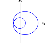
(b) $\gamma=0$, $\alpha=4$.

(c) $\gamma=0$, $\alpha=3/4$.

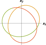
(d) $\gamma=1$, $\alpha=2/3$.

(e) $\gamma=1$, $\alpha=3$.

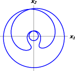
(f) $\gamma=1$, $\alpha=7$.

(g) $\gamma=1/2$, $\alpha=3/4$.

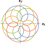
(h) $\gamma=2$, $\alpha=3/4$.

(i) $\gamma=1/3$, $\alpha=3/4$.

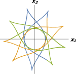
(j) $\gamma=1/3$, $\alpha=5/3$.

(k) $\gamma=3$, $\alpha=5/3$.

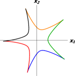
(l) $\gamma=1/3$, $\alpha=3/5$.

Figure 2: Trajectories for some values of the parameters $\alpha$ and $\gamma$. Different colours in the same orbit indicate different branches for the angular variable $\varphi(t)$ according to (3.17). Figures 2(d), 2(e) and 2(f) correspond to examples of the Landau phase $\gamma=1$. In Fig. 2(d) the trajectory encloses the origin of the coordinate system (here, $R_{1}>R_{2}$ and the total change for the period is $\Delta\varphi=4\pi$), contrary to the cases of 2(e) and 2(f) (in which $\Delta\varphi=0$ and $R_{1}<R_{2}$). The last three figures correspond to the trajectories with cusps that occur in the case $R_{1}|\ell_{1}|=R_{2}|\ell_{2}|$.

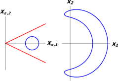
(a) $\alpha=7$, $\gamma=1$, $R_{1}<R_{2}\sin(\pi/\alpha)$.

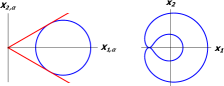
(b) $\alpha=7$, $\gamma=1$, $R_{1}=R_{2}\sin(\pi/\alpha)$.

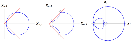
(c) $\alpha=4$, $\gamma=1$, $R_{2}\sin(\pi/\alpha)<R_{1}<R_{2}$.

Figure 3: In Figs. 3(a) and 3(b) the trajectories of the particle in the $(X_{\alpha,1},X_{\alpha,2})$ plane (left) and $(x_{1},x_{2})$ plane (right) are presented. The two red lines indicate the sector of the angle $2\pi/\alpha$, which correspond to the edges of the “cut and flattened” cone space that have to be identified to each other. In Fig. 3(a) the trajectory does not touch these lines, and therefore the particle’s orbit in $(x_{1},x_{2})$ plane is a simple loop. In Fig. 3(b) the trajectory touches the boundaries in the same (identified) point, implying that there is a single point in the $(x_{1},x_{2})$ plane through which the particle passes twice within the period of motion. Finally, the trajectory in the plane $(X_{\alpha,1},X_{\alpha,2})$ crosses the boundaries in Fig. 3(c) (left), and to construct the real trajectory in the “flattened cone” space we use the identity of the edges, and the velocity vector in corresponding points at the edges is constructed by a parallel transport. So when the particle moves from point $a$ to point $b$, it “reappears” at point $b^{\prime}$ on the opposite edge, and moves in the direction of point $c$, and so on. As a result, there are two points on the path in the plane $(x_{1},x_{2})$ through which the particle passes twice within the period of motion. The same logic has to be employed in the analysis of the cases in which the origin of the plane $(X_{\alpha,1},X_{\alpha,2})$ is encircled by the corresponding trajectory.

4 Quantum ERIHO in a conical background

To solve the quantum problem of the conical ERIHO system, we employ the conformal bridge transformation (CBT) in this geometry. Earlier, this technique was used in the study of the quantum isotropic harmonic oscillator in the cosmic string spacetime background [17]. Here, we just very briefly describe the main elements of the construction of ref. [17], in order to apply it then for the study of the quantum conical ERIHO system.

4.1 CBT in a cosmic string background

Consider the quantum version of the conformal symmetry generators (2.15), (2.18) and (2.19), which at $t=0$ are given by

$$\hat{H}^{(\alpha)}_{0}=-\frac{\hbar^{2}}{2m}\left(\frac{1}{\alpha^{2}\rho}\frac{\partial}{\partial\rho}\left(\rho\frac{\partial}{\partial\rho}\right)+\frac{1}{\rho^{2}}\frac{\partial^{2}}{\partial\varphi^{2}}\right)\,,\quad\hat{D}^{(\alpha)}=\frac{-i\hbar}{2}(\rho\frac{\partial}{\partial\rho}+1)\,,\quad\hat{K}^{(\alpha)}=\frac{m\alpha^{2}}{2}\rho^{2}\,.\quad$$ (4.1)

They satisfy the $\mathfrak{so}(2,1)$ algebra,

$$[\hat{D}^{(\alpha)},\hat{H}^{(\alpha)}_{0}]=i\hbar\hat{H}^{(\alpha)}_{0}\,,\qquad[\hat{D}^{(\alpha)},\hat{K}^{(\alpha)}]=i\hbar\hat{K}^{(\alpha)}\,,\qquad[\hat{K}^{(\alpha)},\hat{H}^{(\alpha)}_{0}]=i2\hbar\hat{D}^{(\alpha)}\,.$$ (4.2)

Introduce the non-unitary operators

$$\hat{\mathfrak{S}}=e^{-\frac{\omega}{\hbar}\hat{K}^{(\alpha)}}e^{\frac{1}{2\hbar\omega}\hat{H}^{(\alpha)}_{0}}e^{\frac{i}{\hbar}\ln(2)\hat{D}^{(\alpha)}}\,,\qquad\hat{\mathfrak{S}}^{-1}=e^{-\frac{i}{\hbar}\ln(2)\hat{D}^{(\alpha)}}e^{-\frac{1}{2\hbar\omega}\hat{H}^{(\alpha)}_{0}}e^{\frac{\omega}{\hbar}\hat{K}^{(\alpha)}}\,.$$ (4.3)

They produce a similarity transformation, whose application to generators (4.1) yields

$$\hat{\mathfrak{S}}(\hat{H}^{(\alpha)}_{0},\hat{D}^{(\alpha)},\hat{K}^{(\alpha)})\hat{\mathfrak{S}}^{-1}=(-\hbar\omega\hat{\mathcal{J}}^{(\alpha)}_{-},-i\hbar\hat{\mathcal{J}}_{0}^{(\alpha)},\hbar\omega^{-1}\hat{\mathcal{J}}^{(\alpha)}_{+})\,,$$ (4.4)

where

$$\hat{\mathcal{J}}_{0}^{(\alpha)}=\frac{1}{2\omega\hbar}(\hat{H}^{(\alpha)}_{0}+\omega^{2}\hat{K}^{(\alpha)})\,,\qquad\hat{\mathcal{J}}^{(\alpha)}_{\pm}=-\frac{1}{2\omega\hbar}(\hat{H}^{(\alpha)}_{0}-\omega^{2}\hat{K}^{(\alpha)}\pm 2i\hat{D}^{(\alpha)})\,$$ (4.5)

coincide with the dimensionless quantum version of the integrals $(\mathcal{J}_{0}^{(\alpha)},\mathcal{J}^{(\alpha)}_{\pm})$ taken at $t=0$, which are given by Eqs. (3.19) and (3.37). These operators generate the quantum $\mathfrak{sl}(2,\mathbb{R})$ conformal algebra

$$[\hat{\mathcal{J}}_{0}^{(\alpha)},\hat{\mathcal{J}}^{(\alpha)}_{\pm}]=\pm\hat{\mathcal{J}}^{(\alpha)}_{\pm}\,,\qquad[\hat{\mathcal{J}}^{(\alpha)}_{-},\hat{\mathcal{J}}^{(\alpha)}_{+}]=2\hat{\mathcal{J}}_{0}^{(\alpha)}\,.$$ (4.6)

The dimensionless quantum version of the integral $\mathcal{L}^{(\alpha)}$ is invariant under this transformation,

$$\hat{\mathfrak{S}}(\hat{\mathcal{L}}^{(\alpha)})\hat{\mathfrak{S}}^{-1}=\hat{\mathcal{L}}^{(\alpha)}\,,\qquad\hat{\mathcal{L}}^{(\alpha)}=-i\frac{\alpha}{2}\frac{\partial}{\partial\varphi}\,.$$ (4.7)

The described isotropic similarity transformation in a cosmic string background is useful to solve the quantum problem of an isotropic harmonic oscillator in this geometry [17]. This is because its Hamiltonian is given by

$$\hat{H}_{\text{osc}}^{(\alpha)}=2\omega\hbar\hat{\mathcal{J}}_{0}^{(\alpha)}=-\frac{\hbar^{2}}{2m}\left(\frac{1}{\alpha^{2}\rho}\frac{\partial}{\partial\rho}\left(\rho\frac{\partial}{\partial\rho}\right)+\frac{1}{\rho^{2}}\frac{\partial^{2}}{\partial\varphi^{2}}\right)+\frac{1}{2}m\omega^{2}\alpha^{2}\rho^{2}\,,$$ (4.8)

and $\hat{\mathcal{J}}^{(\alpha)}_{\pm}$ are identified as the second-order radial ladder operators. To find the corresponding energy eigenstates, we apply the operator $\hat{\mathfrak{S}}$ to the states

$$\Omega_{n_{\rho},\ell}^{(\alpha)}=\rho^{2n_{\rho}+\alpha|\ell|}e^{i\ell\varphi}\,,\qquad n_{\rho}=0,2,\ldots\,,\qquad\ell=0,\pm 1,\pm 2\,,\ldots\,,$$ (4.9)

which simultaneously are the Jordan states of zero energy of the free particle Hamiltonian, and the formal eigenstates of the $\mathcal{PT}$-symmetric operator $2i\hat{D}^{(\alpha)}$ with real eigenvalues [29]. These functions satisfy the relations

$$\hat{H}^{(\alpha)}_{0}\Omega_{n_{\rho},\ell}^{(\alpha)}=-2\frac{\hbar^{2}}{m\alpha^{2}}n_{\rho}(n_{\rho}+\alpha|\ell|)\Omega_{n_{\rho}-1,\ell}^{(\alpha)}\,,\qquad\hat{K}^{(\alpha)}\Omega_{n_{\rho},\ell}^{(\alpha)}=\frac{m\alpha^{2}}{2}\Omega_{n_{\rho}+1,\ell}^{(\alpha)}\,,$$ (4.10)

$$2i\hat{D}^{(\alpha)}\Omega_{n_{\rho},\ell}^{(\alpha)}=\hbar(2n_{\rho}+\alpha|\ell|+1)\Omega_{n_{\rho},\ell}^{(\alpha)}\,,\qquad\hat{\mathcal{L}}^{(\alpha)}\Omega_{n_{\rho},\ell}^{(\alpha)}=\frac{\alpha\ell}{2}\Omega_{n_{\rho},\ell}^{(\alpha)}\,.$$ (4.11)

The application of the conformal bridge generator $\hat{\mathfrak{S}}$ from the left to these equations yields

$$\hat{H}_{\text{osc}}^{(\alpha)}\psi_{n_{\rho},\ell}^{(\alpha)}=\hbar\omega(2n_{\rho}+\alpha|\ell|+1)\psi_{n_{\rho},\ell}^{(\alpha)}\,,\qquad\hat{\mathcal{L}}^{(\alpha)}\psi_{n_{\rho},\ell}^{(\alpha)}=\frac{1}{2}\alpha\ell\psi_{n_{\rho},\ell}^{(\alpha)}\,,$$ (4.12)

$$\hat{\mathcal{J}}^{(\alpha)}_{+}\psi_{n_{\rho},\ell}^{(\alpha)}(r,\varphi)=-\sqrt{(n_{\rho}+1)(n_{\rho}+\alpha|\ell|+1)}\psi_{n_{\rho}+1,\ell}^{(\alpha)}(r,\varphi)\,,$$ (4.13)

$$\hat{\mathcal{J}}^{(\alpha)}_{-}\psi_{n_{\rho},\ell}^{(\alpha)}(r,\varphi)=-\sqrt{n_{\rho}(n_{\rho}+\alpha|\ell|)}\psi_{n_{\rho}-1,\ell}^{(\alpha)}(r,\varphi)\,,$$ (4.14)

where we have used relations

$$\hat{\mathfrak{S}}\Omega_{n_{\rho},\ell}^{(\alpha)}(r,\varphi)=\mathcal{N}_{n_{\rho},\ell}^{(\alpha)}\psi_{n_{\rho},\ell}^{(\alpha)}(r,\varphi)\,,$$ (4.15)

$$\mathcal{N}_{n_{\rho},\ell}^{(\alpha)}=(-1)^{n_{\rho}}\left(\frac{2\hbar}{m\omega\alpha^{2}}\right)^{n_{\rho}+\frac{\alpha|\ell|}{2}}\sqrt{\alpha\pi n_{\rho}!\Gamma(n_{\rho}+\alpha|\ell|+1)}\,,$$ (4.16)

and

$$\psi_{n_{\rho},\ell}^{(\alpha)}(\rho,\varphi)=\left(\frac{m\omega\alpha^{2}}{\hbar}\right)^{\frac{1}{2}}\sqrt{\frac{n_{\rho}!}{\pi\alpha\Gamma(n_{\rho}+\alpha|\ell|+1)}}\,\zeta^{\alpha|l|}L_{n_{\rho}}^{(\alpha|\ell|)}(\zeta^{2})e^{-\frac{\zeta^{2}}{2}+i\ell\varphi}\,,\quad\zeta=\sqrt{\frac{m\alpha^{2}\omega}{\hbar}}\rho\,,\quad$$ (4.17)

with $L_{n}^{(\nu)}(z)$ to be the generalized Laguerre polynomials. For more details on application of this technique to other models, see [17, 39, 29]. Here, we just take into account that the Hamiltonian of our conical ERIHO system is a linear combination of the integrals $\mathcal{J}_{0}^{(\alpha)}$ and $\mathcal{L}^{(\alpha)}$, the quantum versions of which are simultaneously diagonalized by wave functions (4.17).

4.2 Quantum conical ERIHO system

The Hamiltonian operator of the quantum conical ERIHO system is given by

$$\begin{array}[]{lll}\hat{H}_{\gamma}^{(\alpha)}&=&2\hbar\omega(\hat{\mathcal{J}}_{0}^{(\alpha)}+\gamma\hat{\mathcal{L}}^{(\alpha)})\\ &=&-\frac{\hbar^{2}}{2m}\left(\frac{1}{\alpha^{2}\rho}\frac{\partial}{\partial\rho}\left(\rho\frac{\partial}{\partial\rho}\right)+\frac{1}{\rho^{2}}\frac{\partial^{2}}{\partial\varphi^{2}}\right)+\frac{m\omega^{2}\alpha^{2}}{2}\rho^{2}-\omega\gamma\alpha i\hbar\frac{\partial}{\partial\varphi}\,.\end{array}$$ (4.20)

Since the structure of this operator is a linear combination of the Hamiltonian of the isotropic harmonic oscillator in the cone [17] and the angular momentum operator, it is easy to show that the eigenstates correspond to (4.17), and the spectrum is

$$E_{n_{\rho},\ell}^{(\alpha,\gamma)}=\hbar\omega(2n_{\rho}+\alpha(1+\gamma\,\text{sign}(\ell))|\ell|+1)\,,$$ (4.21)

$$n_{\rho}=0,1,\ldots\,,\qquad\ell=0,\pm 1,\pm 2,\ldots\,.\qquad$$ (4.22)

Indeed, operator (4.20) can be presented as

$$\hat{H}_{\gamma}^{(\alpha)}=\hat{\mathfrak{S}}2\omega(i\hat{D}^{(\alpha)}+\gamma\hbar\hat{\mathcal{L}}^{(\alpha)})\hat{\mathfrak{S}}^{-1}\,,$$ (4.23)

and then $2\omega(i\hat{D}^{(\alpha)}+\gamma\hbar\hat{\mathcal{L}}^{(\alpha)})\Omega_{n_{\rho},\ell}^{(\alpha)}=E_{n_{\rho},\ell}^{(\alpha,\gamma)}\Omega_{n_{\rho},\ell}^{(\alpha)}$. Note that the spectrum depends on the two parameters $\alpha$ and $\gamma$, but the eigenfunctions depend only on the parameter $\alpha$. When $|\gamma|<1$, the spectrum is always positive and bounded from below. Meanwhile, the system with $|\gamma|>1$ has negative energy levels, and the spectrum is not bounded from below. In the Landau phases $\gamma=\pm 1$, $E\geq\hbar\omega>0$, and each energy level is infinite degenerate since $(1+\gamma\text{sign}(\ell))$ can vanish for an infinite set of different eigenstates. We will return to this point in the next subsection.

We also find that, according to equations (4.13), (4.14), $\hat{\mathcal{J}}^{(\alpha)}_{\pm}$ are still radial ladder operators. Let us look now for other well defined operators. To this aim, we introduce a new notation for the eigenstates and the spectrum,

$$\psi_{n_{\rho},l}^{(\alpha,+)}=\psi_{n_{\rho},l}^{(\alpha)}\,,\qquad\psi_{n_{\rho},l}^{(\alpha,-)}=\psi_{n_{\rho},-l}^{(\alpha)}\,,\qquad E_{n_{\rho},l}^{(\alpha,\gamma,\pm)}=E_{n_{\rho},\pm l}^{(\alpha,\gamma)}\,,\qquad l=|\ell|\,.$$ (4.24)

With this notation, it is clear that the discrete formal transformation $\sigma:l\rightarrow-l$ produces the functions

$$\sigma(\psi_{n_{\rho},l}^{(\alpha,\pm)})=\left(\frac{m\omega\alpha^{2}}{\hbar}\right)^{\frac{1}{2}}\sqrt{\frac{n_{\rho}!}{\pi\alpha\Gamma(n_{\rho}-\alpha l+1)}}\,\zeta^{-\alpha l}L_{n_{\rho}}^{(-\alpha l)}(\zeta^{2})e^{-\frac{\zeta^{2}}{2}\mp il\varphi}\,,$$ (4.25)

which cannot be physical eigenstates in the general case. Only when $\alpha=q=1,2,\ldots$, the identity

$$\frac{(-\eta)^{i}}{i!}L_{n}^{(i-n)}(\eta)=\frac{(-\eta)^{n}}{n!}L_{i}^{(n-i)}(\eta)\,,\qquad i,n=0,1,\ldots,$$ (4.26)

allows us to show that

$$\sigma(\psi_{n_{\rho},l}^{(q,\pm)})=\left\{\begin{array}[]{lll}(-1)^{lq}\psi_{n_{\rho}-lq,l}^{(q,\mp)}&\text{when}&n_{\rho}\geq ql\\ \\ 0&\text{otherwise }\end{array}\right.\,,\qquad\sigma(E_{n_{\rho},l}^{(q,\gamma,\pm)})=E_{n_{\rho}-ql,l}^{(q,\gamma,\mp)}\,.$$ (4.27)

Therefore, if the action of a certain operator on a particular eigenstate in the physical Hilbert space can produce an eigenstate with negative lower second index, we conclude that such operator is well defined only when $\alpha$ is an integer number. This helps us to see the quantum anomaly.

Now, consider the formal operators

$$\hat{b}_{\alpha,1}^{-}=\frac{1}{2}e^{-i\frac{\varphi}{\alpha}}\sqrt{\frac{m\omega}{\hbar}}\left(\alpha\rho+\frac{\hbar}{m\omega\alpha}\left(\frac{\partial}{\partial\rho}-\frac{i\alpha}{\rho}\frac{\partial}{\partial\varphi}\right)\right)\,,\qquad\hat{b}_{\alpha,1}^{+}=(\hat{b}_{\alpha,1})^{\dagger}\,,$$ (4.28)

$$\hat{b}_{\alpha,2}^{-}=\frac{1}{2}e^{i\frac{\varphi}{\alpha}}\sqrt{\frac{m\omega}{\hbar}}\left(\alpha\rho+\frac{\hbar}{m\omega\alpha}\left(\frac{\partial}{\partial\rho}+\frac{i\alpha}{\rho}\frac{\partial}{\partial\varphi}\right)\right)\,,\qquad\hat{b}_{\alpha,2}^{+}=(\hat{b}_{\alpha,2}^{-})^{\dagger}\,.$$ (4.29)

They are obtained via the conformal bridge transformation,

$$\mathfrak{\hat{S}}(\hat{\Xi}_{+}^{(\alpha)},\hat{\Xi}_{-}^{(\alpha)},\hat{\Pi}_{+}^{(\alpha)},\hat{\Pi}_{-}^{(\alpha)})\mathfrak{\hat{S}}^{-1}=(\sqrt{\frac{2m\hbar}{\omega}}\hat{b}_{\alpha,1}^{+},\sqrt{\frac{2m\hbar}{\omega}}\hat{b}_{\alpha,2}^{+},-i\sqrt{2m\hbar\omega}\hat{b}_{\alpha,2}^{-},-i\sqrt{2m\hbar\omega}\hat{b}_{\alpha,1}^{-})\,,\qquad$$ (4.30)

applied to the free particle formal momenta $\hat{\Pi}_{\pm}^{(q)}$ from (2.56) with $q$ changed for $\alpha$, and Galilean boost generators taken at $t=0$, see ref. [17],

$$\hat{\Xi}_{\pm}^{(\alpha)}=\alpha m\rho e^{i\frac{\varphi}{\alpha}}\,.$$ (4.31)

To find the action of operators (4.28) and (4.29) and some powers of them on the eigenstates $\psi_{n_{\rho},\l}^{(\alpha,\pm)}$, we first compute the action of (2.56) and (4.31) on functions $\Omega_{n_{\rho},\ell}^{(\alpha)}$, and then we use the relations (4.15) and (4.30). As a result we get

$$(\hat{b}_{\alpha,1}^{\pm})^{j}\,\psi_{n_{\rho},l}^{(\alpha,+)}(\rho,\varphi)=\sqrt{\frac{\Gamma(n_{\rho}+\alpha l+1+\beta_{\pm}j)}{\Gamma(n_{\rho}+\alpha l+1-\beta_{\mp}j)}}\,\psi_{n_{\rho},l\pm\frac{j}{\alpha}}^{(\alpha,+)}(\rho,\varphi)\,,\qquad\beta_{\pm}=\frac{1\pm 1}{2}\,,$$ (4.32)

$$(\hat{b}_{\alpha,1}^{\pm})^{j}\,\psi_{n_{\rho},l}^{(\alpha,-)}(\rho,\varphi)=(-1)^{j}\sqrt{\frac{\Gamma(n_{\rho}+1+\beta_{\pm}j)}{\Gamma(n_{\rho}+1-\beta_{\mp}j)}}\,\psi_{n_{\rho}\pm j,l\mp\frac{j}{\alpha}}^{(\alpha,-)}(\rho,\varphi)\,,$$ (4.33)

$$(\hat{b}_{\alpha,2}^{\pm})^{j}\,\psi_{n_{\rho},l}^{(\alpha,-)}(\rho,\varphi)=\sqrt{\frac{\Gamma(n_{\rho}+\alpha l+1+\beta_{\pm}j)}{\Gamma(n_{\rho}+\alpha l+1-\beta_{\mp}j)}}\,\psi_{n_{\rho},l\pm\frac{j}{\alpha}}^{(\alpha,-)}(\rho,\varphi)\,,$$ (4.34)

$$(\hat{b}_{\alpha,2}^{\pm})^{j}\,\psi_{n_{\rho},l}^{(\alpha,+)}(\rho,\varphi)=(-1)^{j}\sqrt{\frac{\Gamma(n_{\rho}+1+\beta_{\pm}j)}{\Gamma(n_{\rho}+1-\beta_{\mp}j)}}\,\psi_{n_{\rho}\pm j,l\mp\frac{j}{\alpha}}^{(\alpha,+)}(\rho,\varphi)\,.$$ (4.35)

It is clear that when $j=1$, we obtain a function outside the Hilbert space in general case since the phase factor is multi-valued. When $\alpha=q/k$, we can select $j=q$ in these equations in order to avoid problems with the phase factor, but we still have the problem of quantum anomaly since when $k>l$, we can obtain the wave functions

$$\psi_{n_{\rho},-|k-l|}^{(\frac{q}{k},\pm)}(\rho,\varphi)=\sigma(\psi_{n_{\rho},|k-l|}^{(\frac{q}{k},\mp)}(\rho,\varphi))\,$$

on the right hand side of the corresponding equation. They will be physical eigenstates only when $k=1$, see Eq. (4.27).

The action of operators $\hat{\mathcal{J}}^{(\alpha)}_{\pm}=\hat{b}_{1,\alpha}^{\pm}\hat{b}_{2,\alpha}^{\pm}$ (that is an equivalent form of the second definition in (4.5)) on eigenstates $\psi_{n_{\rho},l}^{(\alpha,\pm)}$ produces a change of the radial quantum number $n_{\rho}$ (without touching $l$) for arbitrary values of $\alpha$. Besides, exceptionally when $\alpha=q$, we have the well defined ladder operators $(\hat{b}_{q,i}^{\pm})^{q}$, which allow to change the angular momentum quantum number. In conclusion, only in this last case we can have a spectrum generating set of the ladder operators $(\hat{\mathcal{J}}^{(q)}_{\pm},(\hat{b}_{q,i}^{\pm})^{q})$, whose combined action allows us to generate from a given eigenstate all the physical eigenstates that constitute a basis of the physical Hilbert space. On the other hand, operators $\hat{b}_{\alpha,i}^{\pm}$ are the building blocks for the construction of any symmetry operator that correctly explains the emergent degeneracy of the spectrum in dependence on the values of the parameters $\alpha$ and $\gamma$. According to our previous analysis, this construction is only possible when $\alpha$ takes a positive integer value, that we imply from now on.

Until now, the construction is valid for arbitrary values of the parameter $\gamma$.

4.3 Spectral degeneracy

Case $\gamma=\frac{s_{2}-s_{1}}{s_{2}+s_{1}}$. The quantum version of (3.26) corresponds to the operators

$$\hat{\mathscr{L}}_{q,s_{1},s_{2}}^{(\epsilon)+}=(\hat{b}_{1,q}^{+})^{s_{1}\epsilon}(\hat{b}_{2,q}^{-})^{s_{2}\epsilon}\,,\qquad\hat{\mathscr{L}}_{q,s_{1},s_{2}}^{(\epsilon)-}=(\hat{\mathscr{L}}_{q,s_{1},s_{2}}^{(\epsilon)+})^{\dagger}\,.$$ (4.36)

They are obtained via conformal bridge transformation (up to an inessential multiplicative constant), from the higher order free particle symmetry operators

$$\hat{\mathscr{S}}_{q,s_{1},s_{2}}^{(\epsilon)+}=(\hat{\Xi}_{+}^{(q)})^{s_{1}\epsilon}(\hat{\Pi}_{+}^{(q)})^{s_{2}\epsilon}\,,\qquad\hat{\mathscr{S}}_{q,s_{1},s_{2}}^{(\epsilon)-}=(\hat{\Pi}_{-}^{(q)})^{s_{1}\epsilon}(\hat{\Xi}_{-}^{(q)})^{s_{2}\epsilon}\,,$$ (4.37)

which commute with the combination $2\omega(i\hat{D}^{(q)}+\gamma\hbar\hat{\mathcal{L}}^{(q)})$ for the chosen value of the parameter $\gamma=(s_{2}-s_{1})/(s_{2}+s_{1})$.

The action of these operators is given by

$$\hat{\mathscr{L}}_{q,s_{1},s_{2}}^{(\epsilon)\pm}\psi_{n_{\rho},l}^{(q,+)}=(-1)^{\epsilon s_{2}}\sqrt{\frac{\Gamma(n_{\rho}+1+\beta_{\mp}\epsilon s_{2})}{\Gamma(n_{\rho}+1-\beta_{\pm}\epsilon s_{2})}\frac{\Gamma(n_{\rho}+ql+1+\beta_{\pm}\epsilon s_{1})}{\Gamma(n_{\rho}+ql+1-\beta_{\mp}\epsilon s_{1})}}\psi_{n_{\rho}\mp\epsilon s_{2},l\pm\frac{\epsilon(s_{1}+s_{2})}{q}}^{(q,+)}\,,$$ (4.38)

$$\hat{\mathscr{L}}_{q,s_{1},s_{2}}^{(\epsilon)\mp}\psi_{n_{\rho},l}^{(q,-)}=(-1)^{\epsilon s_{1}}\sqrt{\frac{\Gamma(n_{\rho}+1+\beta_{\mp}\epsilon s_{1})}{\Gamma(n_{\rho}+1-\beta_{\pm}\epsilon s_{1})}\frac{\Gamma(n_{\rho}+ql+1+\beta_{\pm}\epsilon s_{2})}{\Gamma(n_{\rho}+ql+1-\beta_{\mp}\epsilon s_{2})}}\psi_{n_{\rho}\mp\epsilon s_{1},l\pm\frac{\epsilon(s_{1}+s_{2})}{q}}^{(q,-)}\,.$$ (4.39)

In accordance with Eq. (3.26), the value of the parameter $\epsilon$ guarantees that $\epsilon/q$ is integer. We conclude then that these operators are responsible for the degeneracy of the system since the energy eigenvalues satisfy the relations

$$E_{n_{\rho},l}^{(q,\gamma,+)}=E_{n_{\rho}-\epsilon s_{2},l+\frac{\epsilon(s_{1}+s_{2})}{q}}^{(q,\gamma,+)}=E_{n_{\rho}+\epsilon s_{2},l-\frac{\epsilon(s_{1}+s_{2})}{q}}^{(q,\gamma,+)}\,,$$ (4.40)

$$E_{n_{\rho},-l}^{(q,\gamma,-)}=E_{n_{\rho}-\epsilon s_{1},-l+\frac{\epsilon(s_{1}+s_{2})}{q}}^{(q,\gamma,-)}=E_{n_{\rho}+\epsilon s_{1},l-\frac{\epsilon(s_{1}+s_{2})}{q}}^{(q,\gamma,-)}\,.$$ (4.41)

The poles of the Gamma functions and relation (4.27) guarantee that only physical eigenstates are produced by the action of these operators.

When $\gamma=1$ ($s_{1}=s_{2}=1$), equations (4.38), (4.39) are reduced to equations (6.57), (6.58) of [17] when $q$ is even ($\epsilon=q/2$), and to (6.59), (6.60) when $q$ is odd ($\epsilon=q$). On the other hand, when $q=1$ ($\epsilon=1$), the integrals (4.36) are reduced to the integrals of the Euclidean quantum ERIHO system described in ref. [39]. Precisely, another way to obtain the integrals (4.36) is first applying the quantum version of the canonical transformation (3.5) to the integrals of the Euclidean case, and then taking the power $\epsilon$ of the resulting objects, just as it was done at the classical level.

Case $\gamma=\frac{s_{2}+s_{1}}{s_{2}-s_{1}}$. The quantum version of (3.26) corresponds to

$$\hat{\mathscr{J}}_{q,s_{1},s_{2}}^{(\delta)+}=(\hat{b}_{1,q}^{+})^{s_{1}\delta}(\hat{b}_{2,q}^{+})^{s_{2}\delta}\,,\qquad\hat{\mathscr{J}}_{q,s_{1},s_{2}}^{(\delta)-}=(\hat{\mathscr{J}}_{q,s_{1},s_{2}}^{(\delta)+})^{\dagger}\,.$$ (4.42)

These operators are obtained (up to a numerical factor) after the application of the conformal bridge transformation to the higher order operators

$$\hat{\mathscr{T}}_{q,s_{1},s_{2}}^{(\delta)+}=(\hat{\Xi}_{+}^{(q)})^{s_{1}\delta}(\hat{\Xi}_{-}^{(q)})^{s_{2}\delta}\,,\qquad\hat{\mathscr{T}}_{q,s_{1},s_{2}}^{(\delta)-}=(\hat{\Pi}_{-}^{(q)})^{s_{1}\delta}(\hat{\Pi}_{+}^{(q)})^{s_{2}\delta}\,,$$ (4.43)

which commute with $2\omega(i\hat{D}^{(q)}+\gamma\hbar\hat{\mathcal{L}}^{(q)})$ for the chosen value of $\gamma=(s_{2}+s_{1})/(s_{2}-s_{1})$. In the same way as for the previous case, these integrals can also be obtained from their version in the Euclidean case $(\alpha=1)$ [39] by the application of the quantum version of the canonical transformation (3.5) and by taking then the power $\epsilon$ of the resulting objects.

Their action on eigenstates is

$$\hat{\mathscr{J}}_{q,s_{1},s_{2}}^{(\delta)\pm}\psi_{n_{\rho},l}^{(q,+)}=(-1)^{\delta s_{2}}\sqrt{\frac{\Gamma(n_{\rho}+1+\beta_{\pm}\delta s_{2})}{\Gamma(n_{\rho}+1-\beta_{\mp}\delta s_{2})}\frac{\Gamma(n_{\rho}+ql+1+\beta_{\pm}\delta s_{1})}{\Gamma(n_{\rho}+ql+1-\beta_{\mp}\delta s_{1})}}\psi_{n_{\rho}\pm\delta s_{2},l\mp\frac{\delta(s_{2}-s_{1})}{q}}^{(q,+)}\,,$$ (4.44)

$$\hat{\mathscr{J}}_{q,s_{1},s_{2}}^{(\delta)\pm}\psi_{n_{\rho},l}^{(q,-)}=(-1)^{\delta s_{1}}\sqrt{\frac{\Gamma(n_{\rho}+1+\beta_{\pm}\delta s_{1})}{\Gamma(n_{\rho}+1-\beta_{\mp}\delta s_{1})}\frac{\Gamma(n_{\rho}+ql+1+\beta_{\pm}\delta s_{2})}{\Gamma(n_{\rho}+ql+1-\beta_{\mp}\delta s_{2})}}\psi_{n_{\rho}\pm\delta s_{1},l\pm\frac{\delta(s_{2}-s_{1})}{q}}^{(q,-)}\,.$$ (4.45)

Again, $\delta/q$ is an integer number here, and these operators reflect the spectral degeneracy according to the relations

$$E_{n_{\rho},l}^{(q,\gamma,+)}=E_{n_{\rho}+\delta s_{2},l-\frac{\delta(s_{2}-s_{1})}{q}}^{(q,\gamma,+)}=E_{n_{\rho}-\delta s_{2},l+\frac{\delta(s_{2}-s_{1})}{q}}^{(q,\gamma,+)}\,,$$ (4.46)

$$E_{n_{\rho},-l}^{(q,\gamma,-)}=E^{(q,\gamma,-)}_{n_{\rho}+\delta s_{1},l+\frac{\delta(s_{2}-s_{1})}{q}}=E^{(q,\gamma,-)}_{n_{\rho}-\delta s_{1},l-\frac{\delta(s_{2}-s_{1})}{q}}\,.$$ (4.47)

Here, the poles in the Gamma function appear only in the action of the operator $\hat{\mathscr{J}}_{q,s_{1},s_{2}}^{(\delta)-}$, that reflects the infinite degeneracy of the system.

Now let us see in detail how this scheme works in the case of the Landau phases $\gamma=\pm 1$. First, in the case $\gamma=-1$ ($s_{1}=1,s_{2}=0,\epsilon=q$) the equations (4.38), (4.39) reduce to

$$\hat{\mathscr{L}}_{q,1,0}^{(q)\pm}\psi_{n_{\rho},l}^{(q,-)}=(-1)^{q}\sqrt{\frac{\Gamma(n_{\rho}+1+q\beta_{\pm})}{\Gamma(n_{\rho}+1-q\beta_{\mp})}}\psi_{n_{\rho}\pm q,l\mp 1}^{(q,-)}\,,$$ (4.48)

$$\hat{\mathscr{L}}_{q,1,0}^{(q)\pm}\psi_{n_{\rho},l}^{(q,+)}=\sqrt{\frac{\Gamma(n_{\rho}+q(l+\beta_{\pm})+1)}{\Gamma(n_{\rho}+q(l-\beta_{\mp})+1)}}\psi_{n_{\rho},l\pm 1}^{(q,+)}\,,$$ (4.49)

while for $\gamma=1$ ($s_{1}=0,s_{1}=1,\epsilon=q$), we get

$$\hat{\mathscr{L}}_{q,0,1}^{(q)\pm}\psi_{n_{\rho},l}^{(q,+)}=(-1)^{q}\sqrt{\frac{\Gamma(n_{\rho}+1+q\beta_{\mp})}{\Gamma(n_{\rho}+1-q\beta_{\pm})}}\psi_{n_{\rho}\mp q,l\pm 1}^{(q,+)}\,,$$ (4.50)

$$\hat{\mathscr{L}}_{q,0,1}^{(q)\pm}\psi_{n_{\rho},l}^{(q,-)}=\sqrt{\frac{\Gamma(n_{\rho}+q(l+\beta_{\mp})+1)}{\Gamma(n_{\rho}+q(l-\beta_{\pm})+1)}}\psi_{n_{\rho},l\mp 1}^{(q,-)}\,.$$ (4.51)

Then, for the case $\gamma=-1$ ($\gamma=1$), equation (4.49) (Eq. (4.51)) shows us that the energy levels are infinitely degenerate, since the operator $\hat{\mathscr{L}}_{q,1,0}^{(q)+}$ ($\hat{\mathscr{L}}_{q,0,1}^{(q)-}$) works as the raising ladder operator for the quantum number $l$ when it acts on the states of the form $\psi_{n_{\rho},l}^{(q,+)}$ ($\psi_{n_{\rho},l}^{(q,-)})$ without annihilating any of them.

In this section we applied the conformal bridge transformation to identify the special characteristics of the integrals of the quantum conical ERIHO system in a direct way. In spite of our initial motivation to solve the anomaly problem by introducing an additional parameter into the dynamics, the model still carries the same quantum anomaly problem in the conical background in the case of rational non-integer values of $\alpha$ [17]. We observed that there is an interplay between the geometric conical parameter $\alpha$ and the real parameter $\gamma$, which characterizes the ratio of frequencies associated with the isotropic harmonic potential term and the rotational speed of the corresponding cosmic string spacetime. This interplay is revealed first in the quantum spectrum of the model, that degenerates only in the case when both parameters are rational and, secondly, in the integrals of motion, whose definition depends on both parameters, and which can only be constructed when $\alpha$ is a positive integer. In the special case of $\gamma^{2}=1$ we obtained the two quantum Landau phases in the conical background, and identified their corresponding integrals of motion. As these phases are generated by application of the conformal bridge transformation to the free particle in the conical background, the quantum Landau problem on the cone is anomaly free only in the same cases of integer values of the parameter $\alpha=q$.

5 A multi-particle generalization: vortices

It is a theoretical and experimental fact that the two dimensional multi-particle bosonic systems confined by (isotropic or anisotropic) harmonic traps in a rotating reference frame can experience Bose-Einstein condensation at low-temperatures [42, 43]. In the case of isotropic harmonic traps, the Hamiltonian of such a system has the form of the sum of $N$ planar ERIHO Hamiltonians plus an interaction term which can represent the particles collision or a sort of electromagnetic interaction between them. The condensation occurs when this interaction potential is weak and the harmonic trap is stronger than the centrifugal force, i.e., when $|\gamma|\leq 1$ [42]. A special characteristics of the corresponding condensate wave function is the emergence of quantum vortices, which in dependence on the form of the interaction term are expected to be distributed in regular lattices [42, 43]. Having noted that the shape of the classical and quantum solutions of the ERIHO system depends essentially on the geometric background characterized by the cone parameter $\alpha$, it is interesting to see if there is any effect of it at the level of multi-particle systems. In particular, we would like to see what happens with the formation of vortices in the wave function of the condensate in this space. To this aim, in this section we first briefly review the elements of Gross-Pitaevskii formalism to apply it to the condensate wave function in conical geometry. Then, we analyze in detail the simplest case $\gamma^{2}=1$, corresponding to the Landau phases of the conical ERIHO model.

Let us start with the bosonic Hamiltonian of the multi-particle conical ERIHO system

$$\hat{\mathcal{H}}=\sum_{n=1}^{N}H_{\gamma}^{(\alpha)}(\boldmathe{r}_{i})+\mathcal{U}(\boldmathe{r}_{1},\ldots,\boldmathe{r}_{N})\,,\qquad\mathcal{U}(\boldmathe{r}_{1},\ldots,\boldmathe{r}_{N})=\sum_{i<j}U(\boldmathe{r}_{i},\boldmathe{r}_{j})\,,$$ (5.1)

where we have introduced a pairwise interaction between particles. It could be chosen, for example, in the form of the contact potential derived in the Hartree-Fock approximation for alkali gases [49, 50],

$$U(\boldmathe{r}_{i},\boldmathe{r}_{j})=\frac{4\pi\hbar a_{s}}{m}\delta(\boldmathe{r}_{i}-\boldmathe{r}_{j})\,,$$ (5.2)

which we assume from now on. Here, $m$ is interpreted as the reduced mass and the scattering length parameter $a_{s}$ is assumed to be small [49, 43, 50].

To analyze this system we follow the Gross-Pitaevskii formalism [49, 43, 50, 42]. The first step is to perform a second quantization, obtaining as a result the Hamiltonian

$$\hat{\mathcal{H}}=\int dV\hat{\Psi}^{\dagger}\left(\hat{H}_{\gamma}^{(\alpha)}(\boldmathe{r})\right)\hat{\Psi}+\frac{1}{2}\int dVdV^{\prime}\hat{\Psi}^{\dagger}(r)\hat{\Psi}^{\dagger}(r^{\prime})U(\boldmathe{r},\boldmathe{r}^{\prime})\hat{\Psi}(r)\hat{\Psi}(r^{\prime})\,,\,\,\,\,dV=\alpha\rho d\rho d\varphi\,,$$ (5.3)

where the field operators $\hat{\Psi}(\boldmathe{r})=\sum_{\lambda}\psi_{\lambda}(\boldmathe{r})\hat{a}_{\lambda}$ and $\hat{\Psi}^{\dagger}(\boldmathe{r})=\sum_{\lambda}\psi_{\lambda}^{*}(\boldmathe{r})\hat{a}_{\lambda}^{\dagger}$ are constructed in terms of a single particle wave-function $\psi_{\lambda}(\boldmathe{r})$. Here $\lambda$ represents a set of quantum numbers, the annihilation and creation operators of the Fock space are used to describe the quantum state of the system made up of a variable or indeterminate number of particles, and $[\hat{\Psi}(\boldmathe{r}),\hat{\Psi}^{\dagger}(\boldmathe{r}^{\prime})]=\delta(\boldmathe{r}-\boldmathe{r}^{\prime})$. The time evolution equation for $\hat{\Psi}(\boldmathe{r})$ is given by

$$i\hbar\frac{\partial}{\partial t}\hat{\Psi}=[\hat{\Psi},\hat{\mathcal{H}}]=\left(\hat{H}_{\gamma}^{(\alpha)}(\boldmathe{r})+\int dV^{\prime}\hat{\Psi}^{\dagger}(r^{\prime})U(\boldmathe{r},\boldmathe{r}^{\prime})\hat{\Psi}(r^{\prime})\right)\hat{\Psi}(\boldmathe{r})\,.$$ (5.4)

At very low temperature, the field operator can be approximated by its mean value $\psi=\langle\hat{\Psi}\rangle$, which is called the order parameter, or the condensate wave-function [49, 43, 42]. By taking into account the potential (5.2), we arrive at a non-linear Schrödinger equation in a conical space

$$i\hbar\frac{\partial}{\partial t}\psi=\left(\hat{H}_{\gamma}^{(\alpha)}+\frac{4\pi\hbar a_{s}}{m}|\psi|^{2}\right)\psi\,.$$ (5.5)

To have Bose-Einstein condensate at low temperature, the ground energy level should be equal to the chemical potential $\mu$, and function $\psi$ should satisfy $\int dV|\psi|^{2}=N$ (assuming that the number of particles in the condensate is $N_{c}\sim N$). Therefore $|\psi|^{2}=n(\boldmathe{r})$ is understood as the particle density in the condensate, and the anzats $\psi(\boldmathe{r},t)=e^{-i\frac{\mu}{\hbar}t}\psi(\boldmathe{r})$ gives us the stationary version of (5.5),

$$\mu\psi(\boldmathe{r})=\left(\hat{H}_{\gamma}^{(\alpha)}+\frac{4\pi\hbar a_{s}}{m}|\psi|^{2}\right)\psi(\boldmathe{r})\,.$$ (5.6)

Finally, for the case $a_{s}\sim 0$, one can use the variational method to approximate the ground state, which should be close to the ground state of the single particle system.

The interesting cases to see here are $\gamma=1$ and $\gamma=-1$, both of them corresponding to the Landau phases of our conical ERIHO system, with different orientations of the homogeneous magnetic field. Since the ground state is infinitely degenerate, in the case $\gamma_{\pm}=\pm 1$ the solution of (5.6) is approximated by

$$\psi^{(\alpha,\gamma_{\pm})}=\sqrt{N}\sum_{l=0}^{l_{\text{cut}}}c_{l}\psi_{0,l}^{(\alpha,\pm)}\,,\qquad\sum_{l=0}^{l_{\text{cut}}}c_{l}c_{l}^{*}=1\,,$$ (5.7)

where $l_{\text{cut}}$ is a cut-off introduced by hand, and the usual criteria to select the complex constants $c_{l}$ is by minimizing the non-linear potential term expectation value $\frac{4\pi\hbar a_{s}}{m}\int\alpha rdrd\varphi|\psi^{(\alpha)}|^{4}$. Note that the structure of this function is a polynomial in the variable $r^{\alpha}e^{i\varphi}$ (times a Gaussian term) of degree $l_{\text{cut}}$. In the planar case, the corresponding nodes of this function represent quantized vortices in a superfluid, and here this also can happen, but now the influence of geometry of the space is expected to be essential. This is more clear by following the Onsager and Feynman ideas [51, 52], and selecting the solution of (5.5) in the form

$$\psi=\sqrt{n(\boldmathe{r},t)}e^{i\theta(\boldmathe{r},t)}\,.$$ (5.8)

By introducing this anzats, and ignoring the non-linear term, we get the following two equations

$$\frac{\partial}{\partial t}n(\boldmathe{r},t)=\nabla_{c}\cdot(n(\boldmathe{r},t)\boldmathe{v})\,,$$ (5.9)

$$\frac{\partial}{\partial t}\Phi+\frac{1}{2}v^{2}+\frac{P}{m}=0\,,$$ (5.10)

where

$$\Phi=\frac{\hbar\theta}{m}\,,\qquad\boldmathe{v}=\nabla_{c}\Phi-\frac{q}{m}\boldmathe{A}\,,\qquad P=-\frac{\hbar^{2}}{2m}\frac{1}{\sqrt{n}}\nabla_{c}\cdot\left(\nabla_{c}\sqrt{n}\right)\,,$$ (5.11)

and $\nabla_{c}$ is the curvilinear gradient operator that acting on a scalar function $F$ and a vector field $\boldmathe{G}$ yields

$$\nabla_{c}F=\frac{1}{\alpha}\frac{\partial F}{\partial\rho}\boldmathe{e}_{r}+\frac{1}{\rho}\frac{\partial F}{\partial\varphi}\boldmathe{e}_{\varphi}\,,\quad\nabla_{c}\cdot\boldmathe{G}=\frac{1}{\alpha\rho}\frac{\partial(\rho G_{\rho})}{\partial\rho}+\frac{1}{\rho}\frac{\partial G_{\varphi}}{\partial\varphi}\,,$$ (5.12)

$$\nabla_{c}\crossproduct\boldmathe{G}=\left[\frac{1}{\alpha\rho}\frac{\partial(\rho G_{\varphi})}{\partial\rho}-\frac{1}{\rho}\frac{\partial G_{\rho}}{\partial\varphi}\right]\boldmathe{e}_{z}\,,\qquad\nabla_{c}\cdot(\nabla_{c}F)=\frac{1}{\alpha^{2}\rho}\frac{\partial}{\partial\rho}\left(\rho\frac{\partial F}{\partial\rho}\right)+\frac{1}{\rho^{2}}\frac{\partial^{2}F}{\partial\varphi^{2}}\,.$$ (5.13)

Equation (5.9) has the form of the continuity equation for the particle density, and if we interpret $\Phi$ as a fluid potential, then (5.10) looks like the Bernoulli equation for a charged fluid coupled to a constant magnetic field, but now in a conical vessel space when $\alpha>1$, or for a rotating condensate in the presence of radial dislocations [14] for $\alpha<1$. Then, since in general case $\nabla_{c}\crossproduct(\nabla_{c}F)=0$ for a continuous scalar function $F$, we can only have vortices when $\theta$ has singularities. Therefore, if we manage to write down the function (5.7) in the form (5.8), it is seen that the points where vortices can appear are related to the nodes of (5.7), where phase can not be defined. As we mentioned before, the polynomial structure of the wave function depends on $\alpha$, and this can affect the vortices location with respect to the origin. In order to see this, let us consider the case $l_{\text{cut}}=2$ in (5.7), which gives us the condensate wave-function (in units in which $\frac{m\omega\alpha^{2}}{\hbar}=1$)

$$\psi_{a_{0},a_{1},a_{2}}^{(\alpha)}(\rho,\varphi)=\sqrt{\frac{\alpha N}{\pi(|a_{0}|^{2}+|a_{1}|^{2}+|a_{2}|^{2})}}\left(a_{0}+\frac{a_{1}(\alpha\rho)^{\alpha}}{\sqrt{\Gamma(\alpha+1)}}e^{i\varphi}+\frac{a_{2}(\alpha\rho)^{2\alpha}}{\sqrt{\Gamma(\alpha+1)}}e^{i2\varphi}\right)e^{-\frac{\alpha^{2}\rho^{2}}{2}}\,.\quad$$ (5.14)

Here, $\sum_{0}^{l_{\text{cut}}}c_{l}c_{l}^{*}=1$, where $c_{l}=a_{l}(|a_{0}|^{2}+|a_{1}|^{2}+|a_{2}|^{2})^{-\frac{1}{2}}$, $l=0,1,2$. In Table 1, we present some numerical results for the coefficients $a_{l}$, that were obtained to minimize the integral

$$I_{a_{0},a_{1},a_{2}}=\int_{0}^{\infty}\int_{0}^{2\pi}\alpha\rho d\rho d\varphi|\psi_{a_{0},a_{1},a_{2}}^{(\alpha)}(\rho,\varphi)|^{4}\,.$$ (5.15)

$\alpha$	$a_{0}$	$a_{1}$	$a_{2}$	$I_{a_{0},a_{1},a_{2}}$
$1/4$	$0$	$0$	$1$	$1/(4\pi)\approx 0.025$
$1/3$	$0$	$0$	$1$	$\Gamma(7/6)/(6\pi^{\frac{3}{2}}\Gamma(5/3))\approx 0.031$
$1/2$	$0$	$0$	$1$	$1/(8\pi)\approx 0.040$
$1$	$0$	$0$	$1$	$3/(16\pi)\approx 0.060$
$2$	$1$	$0$	$\sqrt{112/19}\approx 2.428$	$33/(131\pi)\approx 0.080$
$3$	$1$	$0$	$\sqrt{992/199}\approx 2.233$	$115/(397\pi)\approx 0.092$
$4$	$1$	$0$	$\sqrt{32512/6179}\approx 2.294$	$12866/(38691\pi)\approx 0.106$

Table 1: The values of parameters that minimize $I_{a_{0},a_{1},a_{2}}$ for different values of $\alpha$, where $a_{i}$ are assumed to be real numbers (the imaginary part only contributes with a global sign in this particular case). Note that the value of $I_{a_{0},a_{1},a_{2}}$ grows with the increasing value of $\alpha$.

For the cases $0<\alpha\leq 1$, two of the three parameters are zero. So, in these cases the solution of the form (5.14) that minimizes $I_{a_{0},a_{1},a_{2}}$ has only one vortex at the origin of coordinates. On the other hand, when $\alpha>1$, two parameters are non-zero, and as is seen from Figure 4, two vortices appear in the corresponding solutions.

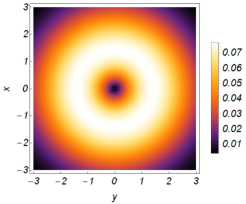
(a) $\alpha=1/2$

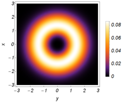
(b) $\alpha=1$

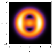
(c) $\alpha=2$

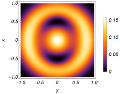
(d) $\alpha=3$

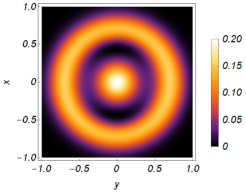
(e) $\alpha=4$

(f) $\alpha=3$

Figure 4: Density plots of the function $|\psi_{a_{0},a_{1},a_{2}}^{(\alpha)}|^{2}/N$ for different values of $\alpha$ are shown in figures from 4(a) to 4(e), and the coefficients $a_{j}$ are chosen according to Table 1. In Fig. 4(f) we consider the density plot of the function $|\psi_{a_{0},a_{1},a_{2},a_{3}}^{(\alpha)}|^{2}/N$ with $\alpha=3$, where the complex values $a_{i}$ with $i=0,\ldots,3$ are such that $I_{a_{0},a_{1},a_{2},a_{3}}=0.073$. Bright (dark) colours indicate maximum (minimum) values of this function. Note that as $\alpha$ grows from $0<\alpha\leq 1$ to $\alpha=2,3,\ldots,$ a local maximum appears in the origin of coordinates and the two appearing vortices seem to degenerate in one single region without particles.

If by hand we put $a_{2}=0$ in function (5.14) and minimize the integral (5.15) for integer values of $\alpha\geq 1$, we get the results presented in Table 2.

$\alpha$	$a_{0}$	$a_{1}$	$I_{a_{0},a_{1},0}$
$1$	$0$	$1$	$1/(4\pi)\approx 0.080$
$2$	$0$	$1$	$3/(8\pi)\approx 0.119$
$3$	$1$	$2\sqrt{3}\approx 3.464$	$6/(13\pi)\approx 0.147$
$4$	$1$	$4\sqrt{7/19}\approx 2.428$	$66/(131\pi)\approx 0.160$

Table 2: The values of the parameters that minimize $I_{a_{0},a_{1},a_{2}=0}$ in dependence on $\alpha$. Note that the values of $I_{a_{0},a_{1},0}$ are greater than the values obtained in the case when $a_{2}\not=0$. When $\alpha$ grows, one vortex has to appear far from the origin.

By comparison of Tables 1 and 2 we learn that the condensate wave-function gives a better approximation to the ground state of (5.6) when more terms in the series are taken into account, i.e., by introducing a higher number of vortices. Also it is observable that when $\alpha$ grows, the local maximum that appears at the origin of the coordinate (the vertex of the cone) corresponds to an accumulation of particles near that point, and this prohibits the formation of vortices there. Then, in contrast to the Euclidean case where there are no special points and the vortex network corresponds to a triangular lattice [42, 43], one can expect that in the conical case any underlying structure should be built around this singular point.

6 Discussion and outlook

In conclusion, we discuss several open problems that seem interesting from the perspective of the obtained results.

1. We began our consideration with the $(3+1)$ dimensional Minkowski space subjected to a uniform rotation with angular velocity $\Omega$ about a fixed axis and introduced the conical singularity by imposing a geometrical constraint. One can note that in the case of $\Omega\not=0$, the spacetime metric (2.7) can be related to the metric of the spinning cosmic string background [14, 53, 54, 55],

$$ds_{\text{sp}}^{2}=-c^{2}(dt+4c^{-4}GJd\varphi)^{2}+\alpha^{2}d\rho^{2}+\rho^{2}d\varphi^{2}\,,$$ (6.1)

where $J$ is the linear angular momentum density of the string. This is achieved by applying the coordinate transformation $d\varphi\rightarrow\frac{1}{2}(d\varphi-2\alpha\Omega dt)$, $dt\rightarrow dt+\frac{1}{2\alpha\Omega}d\varphi$ in (2.7), followed by the identification $J=\frac{c^{4}}{8\alpha\Omega G}$. The peculiarity of this transformation is that it requires the compactification of the time variable since $\varphi=0\cong\varphi=2\pi$ implies that the new time coordinate is periodic, $t\cong t+\pi/(\alpha\Omega)$ [54]. The non-relativistic limit can also be applied to the geodesic motion in background of the spinning cosmic string. For this, we present the action corresponding to the metric (6.1) in the form

$$S_{\text{sp}}=-mc\int\sqrt{-ds_{\text{sp}}^{2}}=-mc^{2}\int\sqrt{1-\frac{1}{c^{2}}\left[\alpha^{2}\dot{\rho}^{2}+(\rho^{2}-\frac{c^{2}}{4\alpha^{2}\Omega^{2}})\dot{\varphi}^{2}-\frac{c^{2}}{\alpha\Omega}\dot{\varphi}\right]}\,dt\,,$$ (6.2)

and take the limit $c\rightarrow\infty$, $\Omega\rightarrow\infty$ in such a way that $c^{2}/\alpha\Omega=\theta=const$. As a result, we obtain Lagrangian of a non-relativistic anyon in the cone background,

$$L_{\text{any}}=\frac{m}{2}\left(\alpha^{2}\dot{\rho}^{2}+\rho^{2}\dot{\varphi}^{2}-\theta\dot{\varphi}\right)\,,$$ (6.3)

which also includes the planar case at $\alpha=1$. The non-relativistic limit we employed is analogous to the Jackiw-Nair procedure considered earlier in the context of relation of the physics of anyons to exotic extension of the planar Galilei group and non-commutative geometry [56, 57, 58]. It would be interesting to study non-relativistic system (6.3) from the perspective of hidden symmetries and quantum anomaly.

2. As we saw, the trajectories of the two-dimensional non-relativistic model in a conical spacetime subjected to a homogeneous rotation can be obtained from the corresponding orbits in the Euclidean plane in the inertial frame system ($\Omega=0$). This can be achieved by applying the time-dependent canonical transformation supplied with an additional $\alpha$-dependent local canonical transformation to produce the cone geometry. In this way we obtained the trajectories that lie on the corresponding finite- or infinite- sheeted Riemann surfaces in dependence on whether the cone parameter $\alpha$ takes a rational or irrational value. This procedure also helped us to obtain the formal integrals, which are the building blocks for the construction of the well defined in phase space symmetry generators in the case of rational values of $\alpha$. As the problem of geometric quantum anomaly arises when we employ the canonical quantization procedure, one may wonder if the Riemann surface structure should play a special role at the quantum level. It seems to be worthing to analyze the problem of the quantum anomaly in more detail by using the method of geometric quantization with taking into account the finite-sheeted Riemann surfaces structure.

3. In the case of geodesic dynamics in non-rotating ($\Omega=0$) cosmic string background with an arbitrary integer value $\alpha=q$ of the geometric parameter we were able to construct the well defined higher order integrals (2.56) that generalize the momenta operators of a free particle in Euclidean geometry, and which reflect correctly the degeneracy of quantum energy levels of the system. By means of the $\Omega$-dependent unitary transformation supplemented by a ‘Heaviside step function regularization’ procedure, we obtained the analogs (2.60) of these integrals, which are non-local operators, and do the same job in the quantum systems with $\alpha=q$ and arbitrary values of the rotation parameter $\Omega\neq 0$. The conformal bridge transformation allowed then us to construct on their basis the analogous integrals for the quantum conical ERIHO systems with integer $\alpha=q$. It is interesting to note here that in the case of the free particle the presence of the frequency parameter $\Omega$ admits the construction of a quantum combination $\hbar\Omega$ of the energy dimension, with which it is possible to regularize by means of the Heaviside step function (whose argument is dimensionless). In the classical theory, the construction of a combination of parameters of the same dimension would require the introduction by hand of an additional constant of the dimension of length.

It would be natural to try to modify somehow the described approach to “cure” the quantum anomaly that still persists in the case of rational values of $\alpha=q/k$ with $k>1$. For this, let us consider first the case of $\Omega=0$, and introduce the alternative integrals

$$\mathfrak{L}_{+}^{(\frac{q}{k})}=\left(\hat{\Pi}_{+}^{(\frac{q}{k})}\right)^{q}\Theta\left(\frac{\hat{p}_{\varphi}}{\hbar}-k\right)\,,\qquad\mathfrak{L}_{-}^{(\frac{q}{k})}=\Theta\left(\frac{\hat{p}_{\varphi}}{\hbar}-k\right)\left(\hat{\Pi}_{-}^{(\frac{q}{k})}\right)^{q}\,.$$ (6.4)

$$\mathfrak{J}_{+}^{(\frac{q}{k})}=\Theta\left(k-\frac{\hat{p}_{\varphi}}{\hbar}\right)\left(\hat{\Pi}_{+}^{(\frac{q}{k})}\right)^{q}\,,\qquad\mathfrak{J}_{-}^{(\frac{q}{k})}=\left(\hat{\Pi}_{-}^{(\frac{q}{k})}\right)^{q}\Theta\left(k-\frac{\hat{p}_{\varphi}}{\hbar}\right)\,.$$ (6.5)

Due to inclusion of the Heaviside step function, these operators do not produce non-physical eigenstates under their application to physical eigenstates. Their explicit action is given by the following relations,

$$\left\{\begin{array}[]{ll}\mathfrak{L}_{+}^{(\frac{q}{k})}\psi_{\kappa,j}^{(\frac{q}{k})}=0\,,&j\leq k-1\\ \\ \mathfrak{L}_{+}^{(\frac{q}{k})}\psi_{\kappa,j}^{(\frac{q}{k})}\sim\psi_{\kappa,j+k}^{(\frac{q}{k})}\,,&j>k-1\end{array}\right.\,,\quad\left\{\begin{array}[]{ll}\mathfrak{L}_{-}^{(\frac{q}{k})}\psi_{\kappa,j}^{(\frac{q}{k})}=0\,,&j\leq 2k-1\\ \\ \mathfrak{L}_{-}^{(\frac{q}{k})}\psi_{\kappa,j}^{(\frac{q}{k})}\sim\psi_{\kappa,j-k}^{(\frac{q}{k})}\,,&j>2k-1\end{array}\right.\,,$$ (6.12)

$$\left\{\begin{array}[]{ll}\mathfrak{J}_{+}^{(\frac{q}{k})}\psi_{\kappa,j}^{(\frac{q}{k})}=0\,,&j\leq k-1\\ \\ \mathfrak{J}_{+}^{(\frac{q}{k})}\psi_{\kappa,j}^{(\frac{q}{k})}\sim\psi_{\kappa,j+k}^{(\frac{q}{k})}\,,&j<k-1\end{array}\right.\,,\quad\left\{\begin{array}[]{ll}\mathfrak{J}_{-}^{(\frac{q}{k})}\psi_{\kappa,j}^{(\frac{q}{k})}=0\,,&j\geq 2k-1\\ \\ \mathfrak{J}_{-}^{(\frac{q}{k})}\psi_{\kappa,j}^{(\frac{q}{k})}\sim\psi_{\kappa,j-k}^{(\frac{q}{k})}\,,&j\geq k-1\end{array}\right.\,,\quad j\in\mathbb{Z}\,.\qquad$$ (6.19)

To generalize for the case with $\Omega\not=0$, we can follow the procedure described in Sec. 2.2. With these two pairs of operators, we have access to all the states with a given energy eigenvalue, except the states of the form $\psi_{\kappa,\ell}^{(\frac{q}{k})}$ with $|\ell|<k-1$. Thus, the question on identifying the symmetry operators that would correctly explain the degeneracy of the energy spectrum when $\alpha$ is rational remains to be open. Perhaps, the operators (6.4) and (6.5) still need to be supplemented with some additional integrals, similar to what happens under the construction of the complete set of the spectrum generating operators in rationally extended harmonic oscillator [59] and rational deformations of conformal mechanics [60].

4. For the harmonic oscillator of frequency $\omega$ in a uniformly rotating cosmic string background, the numerical factor $\gamma=-\Omega/\omega$ can be introduced. This allows us to identify the system as the conical version of the ERIHO model [39, 29], in which closed trajectories and the associated integrals of the hidden symmetry appear when both parameters $\alpha$ and $\gamma$ take rational values. The model reveals a kind of duality under the inversion transformation $\gamma\rightarrow 1/\gamma$ in the same way as this happens in Euclidean version [39]. Namely, in the case $|\gamma|<1$, the system is characterized by a spectrum bounded from bellow, and its true (not depending explicitly on time) symmetry generators satisfy a non-linear version of the $\mathfrak{u}(2)$ algebra. Besides, the system also is characterized by a dynamical non-linear $\mathfrak{gl}(2,\mathbb{R})$ algebra. Additionally, it also is characterized by the conformal $\mathfrak{sl}(2,\mathbb{R})$ symmetry. After applying the duality transformation, we get a system with $|\gamma^{\prime}|=|\gamma^{-1}|>1$, whose quantum spectrum is not bounded from below, and the dynamical (explicitly depending on time) and true symmetries are interchanged, while the conformal $\mathfrak{sl}(2,\mathbb{R})$ symmetry is not changed. In the intermediate case $\gamma^{2}=1$, we use the gravitoelectromagnetic interpretation to identify the model with the Landau problem (in symmetric gauge) in a conical background. The sign of $\gamma$ determines there orientation of the magnetic field. Such a system corresponding to our case $|\gamma|=1$ was considered earlier in [40, 41], where it was shown that some energy levels have infinite degeneracy for arbitrary values of $\alpha$. However, the system was not investigated there in the light of classical and quantum symmetries for special values of the parameter $\alpha$, and this is just a particular case in our analysis. On the other hand, note that the same classical trajectories as we obtained for the case $(0<\alpha<1,\Omega=0)$ were recently observed for geodesics in the conical BTZ spacetimes [61], and it would be interesting to see if the trajectories in the case $\Omega\not=0$ can be related to the dynamics in such a kind of spacetimes as well.

5. Finally, we studied the multi-particle conical ERIHO system in its Landau phases using the mean-field theory. Effectively, we have replaced the pair-wise interaction (that could be a Coulomb one) by a contact potential. The numerical calculation in the simplest examples shows that in the case $0<\alpha\leq 1$ the best approximation of the wave function of the condensate is the one-vortex solution. In the case of $\alpha>1$, the best approximation is obtained by considering multi-vortex configurations, and the accumulation of the particles is possible (while the formation of vortices is prohibited) at the vertex of the cone, where the probability density has a local maximum. Naturally, one may ask if the approximation that we considered is good enough from the point of view of a possible experimental realization, for example by means of the Bose-Einstein condensate in a rotating harmonic trap, or in the system of charged particles subjected to a magnetic field. Anyway, our numerical results indicate that the cone’s vertex should necessarily produce some effect. It would also be interesting to compare these results with a field theory approach, such as the collective field theories, where the large $N$ limit is applied [62]. This problem also is interesting since it can bring some insight into a generalization of the conformal bridge transformation for an infinite number of degrees of freedom.

Acknowledgements

The work was partially supported by the FONDECYT Project 1190842 and the DICYT Project 042131P_POSTDOC.

Appendix A Time-dependent canonical transformation

The system in a rotating flat geometry introduced at the beginning of Section 2 can be obtained from the non-relativistic two-dimensional free particle in the inertial reference frame ($\Omega=0$),

$$S=\int Ldt\,,\qquad L=\frac{m}{2}\frac{d\chi_{i}}{dt}\frac{d\chi_{i}}{dt}\,,\quad\rightarrow\quad H=\frac{1}{2m}\pi_{i}\pi_{i}\,,\qquad\pi_{i}=m\frac{d\chi_{i}}{dt}\,,$$ (A.1)

by applying the time dependent canonical transformation $\chi_{i}\rightarrow x_{i}$, $\pi_{i}\rightarrow p_{i}$, which can be presented in a form

$$x_{\pm}=e^{\mp i\Omega t}\chi_{\pm}=\rho e^{\pm i(\Omega t+\varphi)}\,,\qquad p_{\pm}=e^{\mp i\Omega t}\pi_{\pm}\,.$$ (A.2)

Here $\chi_{\pm}=\chi_{1}\pm i\chi_{2}$, $\pi_{\pm}=\pi_{1}\pm i\pi_{2}$, etc., and $\{\chi_{\pm},\pi_{\pm}\}=0$, $\{\chi_{\pm},\pi_{\mp}\}=2$. Under the time-dependent rotation transformation $\chi_{i}\rightarrow x_{i}$, Lagrangian in (A.1) transforms into Lagrangian (2.4), while the canonical transformation (A.2) applied to the action one-form $\theta=\pi_{i}d\chi^{i}-Hdt$ of the system (A.1) yields $\theta=p_{i}dx^{i}-H_{\Omega}dt$, where $H_{\Omega}$ is the Hamiltonian (2.5). At the same time, the angular momentum is invariant under transformation (A.2), $\pi_{\varphi}=\epsilon_{ij}\chi_{i}\pi_{j}=\epsilon_{ij}x_{i}p_{j}=p_{\varphi}$.

For the system (A.1), canonical momenta are the integrals of motion, $\frac{d}{d\tau}\pi_{\pm}=\{H,\pi_{\pm}\}=0$. On the other hand, according to (A.2), the explicitly depending on time phase space functions

$$P_{\pm}:=e^{\pm i\Omega t}p_{\pm}=\pi_{\pm}$$ (A.3)

are the dynamical integrals of motion for the system $H_{\Omega}$, $\frac{d}{dt}P_{\pm}=\frac{\partial}{\partial t}P_{\pm}+\{P_{\pm},H_{\Omega}\}=0$. Analogously, the explicitly depending on time phase space functions

$$X_{\pm}=e^{\pm i\Omega t}\left(\chi_{\pm}-\frac{1}{m}t\pi_{\pm}\right)$$ (A.4)

are the dynamical integrals of motion for the system $H_{\Omega}$, where $(\chi_{\pm}-\frac{1}{m}t\pi_{\pm})$ are the Galileo boosts generators of the system (A.1). Quadratic rotationally invariant polynomials of (A.3) and (A.4) provide us with the true integrals, $p_{\varphi}=\frac{i}{2}(X_{+}P_{-}-X_{-}P_{+})$ and $H_{\Omega}=H_{0}-\Omega p_{\varphi}$, where $H_{0}=\frac{1}{2m}P_{+}P_{-}$, and the dynamical integrals,

$$D=\frac{1}{4}(X_{+}P_{-}+X_{-}P_{+})=\frac{1}{2}\rho p_{\rho}-H_{0}t\,,$$ (A.5)

$$K=\frac{m}{2}X_{+}X_{-}=\frac{m}{2}\rho^{2}-2Dt-H_{0}t^{2}\,,$$ (A.6)

which correspond to the $\alpha=1$ case of (2.18), (2.19). Multiplying dynamical integrals (A.3) with dynamical integrals $\exp(\pm i\Omega D/H_{0})$, we obtain

$$I_{\pm}^{(1)}=\exp\big(\pm i\Omega\frac{\rho p_{\rho}}{2H_{0}}\big{missing})\cdot p_{\pm}\,.$$ (A.7)

These are the well defined for $H_{0}\neq 0$ true integrals of the system $H_{\Omega}$, to which the integrals (2.32) reduce at $\alpha=1$.

To establish the relation between the quantum Hamiltonians, consider the time-dependent Schrödinger equation for the quantum analog of the system (A.1),

$$i\hbar\frac{\partial}{\partial t}\psi(\chi_{1},\chi_{2},t)=-\frac{\hbar^{2}}{2m}\left(\frac{\partial^{2}}{\partial\chi_{1}^{2}}+\frac{\partial^{2}}{\partial\chi_{1}^{2}}\right)\psi(\chi_{1},\chi_{2},t)\,.$$ (A.8)

Denoting $\Psi(x_{1},x_{2},t)=\Psi(x_{1}(t),x_{2}(t),t)=\psi(\chi_{1},\chi_{2},t)$, where $x_{i}(t)$ are given by the first relation in (A.2), we have $i\frac{\partial}{\partial t}\psi(\chi_{1},\chi_{2},t)=\left(i\hbar\frac{\partial}{\partial t}+\hbar\Omega\hat{p}_{\varphi}\right)\Psi(x_{1},x_{2},t),$ and equation (A.8) takes the form

$$i\hbar\frac{\partial}{\partial t}\Psi(x_{1},x_{2},t)=\hat{H}_{\Omega}\Psi(x_{1},x_{2},t)\,,$$ (A.9)

$$\hat{H}_{\Omega}=-\hbar^{2}\left(\frac{\partial^{2}}{\partial x_{1}^{2}}+\frac{\partial^{2}}{\partial x_{2}^{2}}\right)-\Omega\hat{p}_{\varphi}\,,\qquad\hat{p}_{\varphi}=-i\hbar\left(x_{1}\frac{\partial}{\partial x_{2}}-x_{2}\frac{\partial}{\partial x_{2}}\right)\,.$$ (A.10)

Applying the canonical transformation (3.5), the described procedure can be generalized for the system in conical geometry.

References

- [1] S. L. Adler, “Axial-vector vertex in spinor electrodynamics,” Phys. Rev. 177 (1969) 2426.
- [2] J. S. Bell and R. Jackiw, “A PCAC puzzle: in the -model,” Il Nuovo Cimento A. 60 (1969) 47.
- [3] S. B. Treiman, R. Jackiw, B. Zumino and E. Witten, Current algebras and anomalies (Princeton University Press, 1986).
- [4] R. S. Ward, “Anomalies in conservation laws in quantum mechanics,” Phys. Rev. D 36 (1987) 640.
- [5] B. Carter, “Global structure of the Kerr family of gravitational fields,” Phys. Rev. 174 (1968) 1559.
- [6] G. W. Gibbons, R. H. Rietdijk and J. W. van Holten, “SUSY in the sky,” Nucl. Phys. B 404 (1993) 42 [arXiv:hep-th/9303112].
- [7] M. Cariglia, “Quantum mechanics of Yano tensors: Dirac equation in curved spacetime,” Class. Quant. Grav. 21 (2004) 1051 [arXiv: hep-th/0305153].
- [8] V. P. Frolov and D. Kubiznak, “Hidden symmetries of higher dimensional rotating black holes,” Phys. Rev. Lett. 98 (2007) 011101 [arXiv: gr-qc/0605058].
- [9] V. P. Frolov and D. Kubiznak, “Higher-dimensional black holes: Hidden symmetries and separation of variables,” Class. Quant. Grav. 25 (2008) 154005 [arXiv: 0802.0322 [hep-th]].
- [10] M. Cariglia, V. P. Frolov, P. Krtous and D. Kubiznak, “Geometry of Lax pairs: Particle motion and Killing- Yano tensors,” Phys. Rev. D 87 (2013) 024002 [arXiv:1210.3079 [math-ph]].
- [11] M. Cariglia, “Hidden symmetries of dynamics in classical and quantum physics,” Rev. Mod. Phys. 86 (2014) 1283 [arXiv: 1411.1262 [math-th]].
- [12] V. Frolov, P. Krtous and D. Kubiznak, “Black holes, hidden symmetries, and complete integrability,” Living Rev. Rel. 20 (2017) 6 [arXiv: 1705.05482 [gr-qc]].
- [13] J. M. Bardeen and J. A. Petterson, “The Lense-Thirring effect and accretion disks around Kerr black holes,” Astrophys. J. Lett. 195 (1975) L65.
- [14] G. E. Volovik, The universe in a helium droplet (Oxford Science Publications, 2003).
- [15] B. S. DeWitt, “Quantum field theory in curved spacetime,” Phys. Reports 19 (1975) 295.
- [16] R. M. Wald, Quantum field theory in curved spacetime and black hole thermodynamics (University of Chicago Press, 1994).
- [17] L. Inzunza and M. S. Plyushchay, “Conformal bridge in a cosmic string background,” JHEP 2021 (2021) 165 [arXiv:2012.04613 [hep-th]].
- [18] T. Kibble, “Topology of cosmic domains and strings,” J. Phys. A 9 (1976) 1387.
- [19] A. Vilenkin, “Gravitational field of vacuum domain walls and strings,” Phys. Rev. D 23 (1981) 852.
- [20] A. Vilenkin, “Cosmic strings and domain walls,” Phys. Rept. 121 (1985) 263.
- [21] J. S. Dowker, “Quantum field theory on a cone,” J. Phys. A: Math. Gen. 10 (1977) 115.
- [22] G. ’t Hooft, “Non-perturbative 2 particle scattering amplitudes in 2+1 dimensional quantum gravity,” Commun. Math. Phys. 117 (1988) 685.
- [23] S. Deser and R. Jackiw, “Classical and quantum scattering on a cone,” Comm. Math. Phys 118 (1988) 495.
- [24] B.S. Kay, and U.M. Studer, “Boundary conditions for quantum mechanics on cones and fields around cosmic strings,” Commun. Math. Phys. 139 (1991) 103.
- [25] C. Furtado and F. Moraes, “Harmonic oscillator interacting with conical singularities,” J. Phys. A 33 (2000) 5513.
- [26] J. L. A. Coelho and R. L. P. G. Amaral, “Coulomb and quantum oscillator problems in conical spaces with arbitrary dimensions,” J. Phys. A 35 (2002) 5255 [arXiv: gr-qc/0111114].
- [27] V. de Alfaro, S. Fubini and G. Furlan, “Conformal invariance in quantum mechanics,” Il Nuovo Cimento A (1965-1970) 34 (1976) 569.
- [28] L. Inzunza, M. S. Plyushchay and A. Wipf, “Conformal bridge between asymptotic freedom and confinement,” Phys. Rev. D 101 (2020) 105019 [arXiv:1912.11752 [hep-th]].
- [29] L. Inzunza and M. S. Plyushchay, “Conformal bridge transformation and symmetry,” J. Phys. Conf. Ser. 2038 (2021) 012014 [arXiv:2104.08351 [hep-th]].
- [30] D. Mirfenderesk, J. Raeymaekers, and D. Van den Bleeken, “Superconformal mechanics of AdS 2 D-brane boundstates,” JHEP 2020 (2020) 1.
- [31] H. E. Camblong, A. Chakraborty and C. R. Ordonez, “Near-horizon aspects of acceleration radiation by free fall of an atom into a black hole,” Phys. Rev. D 102 (2020) 085010 [arXiv:2009.06580 [gr-qc]].
- [32] K. Bakke and C. Furtado, “Aharonov-Casher effect in the presence of spin-dependent potential,” Annals Phys. 422 (2020) 168325.
- [33] J. Ben Achour and E. R. Livine, “Cosmological spinor,” Phys. Rev. D 101 (2020) 103523 [arXiv:2004.06387 [gr-qc]].
- [34] J. Anandan and J. Suzuki, “Quantum mechanics in a rotating frame,” In: Rizzi G., Ruggiero M.L. (eds) Relativity in Rotating Frames, Fundamental Theories of Physics, vol. 135 (2004) 361 [arXiv:quant-ph/0305081].
- [35] P. Gulshani and D. J. Rowe, “Quantum mechanics in rotating frames. I. The impossibility of rigid flow,” Can. J. Phys 56 (1978) 468.
- [36] J. E. Brandõ, F. Moraes, M. M. Cunha, J. R. F. Lima and C. Filgueiras, “Inertial-Hall effect: the influence of rotation on the Hall conductivity,” Results Phys. 5 (2015) 55.
- [37] B. L. Johnson, “Inertial forces and the Hall effect,” Am. J. Phys. 68 (2000) 649.
- [38] W. Pauli, “Über das wasserstoffspektrum vom standpunkt der neuen quantenmechanik,” Z. Physik 36 (1926) 336 [“On the hydrogen spectrum from the standpoint of the new quantum mechanics,” In: Dynamical Groups and Spectrum Generating Algebras, p. 369 (1988)].
- [39] L. Inzunza and M. S. Plyushchay, “Conformal generation of an exotic rotationally invariant harmonic oscillator,” Phys. Rev. D 103 (2021) 106004 [arXiv:2103.07752 [quant-ph]].
- [40] G. De A Marques, C. Furtado, V. B. Bezerra and F. Moraes, “Landau levels in the presence of topological defects,” J. Phys. A 34 (2001) 5945 [arXiv:quant-ph/0012146].
- [41] C. R. Muniz, V. B. Bezerra and M. S. Cunha, “Landau quantization in the spinning cosmic string spacetime,” Annals Phys. 350 (2014) 105 [arXiv:1403.6889 [hep-th]].
- [42] N. R. Cooper “Rapidly rotating atomic gases,” Advances in Physics 57 (2008) 539 [arXiv:0810.4398 [cond-mat.mes-hall]].
- [43] A. L. Fetter, “Rotating trapped Bose-Einstein condensates,” Rev. Mod. Phys. 81 (2009) 647 [arXiv:0801.2952 [cond-mat.stat-mech]].
- [44] R. Penrose, “Gravitational collapse: The role of general relativity,” Riv. Nuovo Cim. 1 (1969) 252.
- [45] R. K. Williams, “Collimated escaping vortical polar e- e+ jets intrinsically produced by rotating black holes and Penrose processes,” Astrophys. J. 611 (2004) 952 [arXiv:astro-ph/0404135].
- [46] G. O. Ludwig, “Galactic rotation curve and dark matter according to gravitomagnetism,” Eur. Phys. J. C 81 (2021) 186.
- [47] B. Mashhoon, “Gravitoelectromagnetism: A Brief review,” In: The Measurement of Gravitomagnetism: A Challenging Enterprise, Edited by L. Iorio (Nova Science, New York, 2007), p. 29 [arXiv:gr-qc/0311030].
- [48] J. G. Cramer, R. L. Forward, M. S. Morris, M. Visser, G. Benford, and G. A. Landis, “Natural wormholes as gravitational lenses,” Phys. Rev. D 51 (1995) 3117.
- [49] A. J. Leggett, “Bose-Einstein condensation in the alkali gases: Some fundamental concepts,” Rev. Mod. Phys. 73 (2001) 307.
- [50] K. Huang, Statistical mechanics, 2nd edition (Wiley, New York 1987).
- [51] L. Onsager, “Statistical hydrodynamics,” Il Nuovo Cimento (1943-1954) 6 (1949) 279.
- [52] R. P. Feynman “Application of quantum mechanics to liquid helium,” Progress in Low Temperature Physics. 1 (1955) 17.
- [53] S. Deser, R. Jackiw and G. ’t Hooft, “Three-dimensional Einstein gravity: Dynamics of flat space,” Annals of Phys. 152 (1984) 220.
- [54] P. O. Mazur, “Spinning cosmic strings and quantization of energy,” Phys. Rev. Lett. 57 (1986) 929.
- [55] N. Ozdemir, “Spinning cosmic strings: A general class of solutions,” Int. J. Mod. Phys. A 20 (2005) 2821 [arXiv:gr-qc/0508017].
- [56] R. Jackiw and V. P. Nair, “Anyon spin and the exotic central extension of the planar Galilei group,” Phys. Lett. B 480 (2000) 237 [arXiv: hep-th/0003130].
- [57] P. A. Horvathy and M. S. Plyushchay, “Non-relativistic anyons, exotic Galilean symmetry and noncommutative plane,” JHEP 06 (2002) 033 [arXiv: hep-th/0201228].
- [58] P. A. Horvathy and M. S. Plyushchay, “Anyon wave equations and the noncommutative plane,” Phys. Lett. B 284 (2004) 547 [arXiv: hep-th/0404137].
- [59] J. F. Cariñena and M. S. Plyushchay, “ABC of ladder operators for rationally extended quantum harmonic oscillator systems,” J. Phys. A: Math. Theor. 50 (2017) 275202 [arXiv: 1701.08657 [math-ph]].
- [60] J. F. Cariñena, L. Inzunza and M. S. Plyushchay, “Rational deformations of conformal mechanics,” Phys. Rev. D 98 (2018) 026017 [arXiv: 1707.07357 [math-ph]].
- [61] M. Briceño, C. Martínez and J. Zanelli, “Overspinning naked singularities in AdS3 spacetime,” Phys. Rev. D 104 (2021) 044023 [arXiv:2105.06488 [gr-qc]].
- [62] A. Jevicki and B. Sakita, “The quantum collective field method and its application to the planar limit,” Nucl. Phys. B 165 (1980)511.