Toward Communication Efficient Adaptive Gradient Method

Abstract

In recent years, distributed optimization is proven to be an effective approach to accelerate training of large scale machine learning models such as deep neural networks. With the increasing computation power of GPUs, the bottleneck of training speed in distributed training is gradually shifting from computation to communication. Meanwhile, in the hope of training machine learning models on mobile devices, a new distributed training paradigm called “federated learning” has become popular. The communication time in federated learning is especially important due to the low bandwidth of mobile devices. While various approaches to improve the communication efficiency have been proposed for federated learning, most of them are designed with SGD as the prototype training algorithm. While adaptive gradient methods have been proven effective for training neural nets, the study of adaptive gradient methods in federated learning is scarce. In this paper, we propose an adaptive gradient method that can guarantee both the convergence and the communication efficiency for federated learning.

Keywords:  Federated Learning, Adaptive Method, Optimization, Convergence Analysis

1 Introduction

Distributed training has been proven to be a successful way of accelerating training large scale machine learning models, for example, training ultra-large-scale CTR (click-through rate) models in commercial search engines Fan et al. (2019); Zhao et al. (2020); Xu et al. (2021). With the advances of computing power and algorithmic design, one can now train models that need to be trained for days even weeks in the past within just a few minutes (You et al., 2020). When the computing power is high compared with the network bandwidth connecting different machines in distributed training, the training speed can be bottlenecked by the transmission of gradients and parameters. Such situation occurs increasingly more often in recent years due to the rapid growth in power of GPUs. Therefore, reducing communication overhead is gradually becoming an important research direction in distributed training (Alistarh et al., 2017; Wangni et al., 2018; Lin et al., 2018). In addition, a new training paradigm called Federated Learning (Konečnỳ et al., 2016; McMahan et al., 2017) was proposed recently, where models are trained distributively with mobile devices as workers and data holders. Consider the case where the data is stored and the model is trained on each user’s mobile device (e.g., Wang et al. (2020)). The existence of limited bandwidth necessitates the development of communication efficient training algorithms. Moreover, it is unpractical for every user to keep communicating with the central server, due to the power condition or wireless connection of the device. To cope with communication issues, an SGD-based algorithm with periodic model averaging called Federated Averaging is proposed in McMahan et al. (2017).

Federated learning extends the traditional parameter server setting, where the data are located on different workers and information is aggregated at a central parameter server to coordinate the training. In the parameter server setting, many effective communication reduction techniques were proposed such as gradient compression (Lin et al., 2018; Bernstein et al., 2018) and quantization (Alistarh et al., 2017; Wangni et al., 2018; Wen et al., 2017) for distributed SGD. In federated learning, one can substantially reduce communication cost by avoiding frequent transmission between local workers and central server. The workers train and maintain their own models locally, and the central server aggregates and averages the model parameters of all workers periodically. After averaging, new model parameter is fed back to each local worker, which starts another round of “local training + global averaging”. Some of the aforementioned communication reduction techniques can also be incorporated into Federated Averaging to further reduce the communication cost (Reisizadeh et al., 2020).

Despite the active efforts on improving algorithms based on periodic model averaging (Haddadpour et al., 2019; Reisizadeh et al., 2020; Haddadpour et al., 2020), the prototype algorithm is still SGD. On the other hand, we know that adaptive gradient methods such as AdaGrad (Duchi et al., 2011), Adam (Kingma and Ba, 2015) and AMSGrad (Reddi et al., 2019) often perform better than SGD when training neural nets, in terms of difficulty of parameter tuning and convergence speed at early stages. This motivates us to study adaptive gradient methods in federated learning.

Our contributions. We study how to incorporate adaptive gradient method into federated learning. Specifically, we show that unlike SGD, a naive combination of adaptive gradient methods and periodic model averaging results in algorithms that may fail to converge. Based on federated averaging and decentralized training, we propose an adaptive gradient method with communication cost sublinear in $T$ that is guaranteed to converge to stationary points with a rate of $O(\sqrt{d}/\sqrt{TN})$, where $d$ is the dimension of the problem, $T$ is the number of iterations, and $N$ is the number of workers (nodes). Our proposed method enjoys the benefit from both worlds: the fast convergence performance of adaptive gradient methods and low communication cost of federated learning.

2 Related Work

Federated learning. A classical framework for distributed training is the parameter server framework. In such a setting, a parameter server is used to coordinate training and the main computation (e.g., gradient computation) is offloaded to workers in parallel. For SGD under this framework (Recht et al., 2011; Li et al., 2014; Zinkevich et al., 2010; Zhao et al., 2020), the gradients can be computed by workers on their local data and sent to the parameter server which will aggregate the gradients and update the model parameters. Recently, a variant of the parameter server setting called federated learning (McMahan et al., 2017; Konečnỳ et al., 2016) draws great attention. One of the key features of federated learning is that workers are likely to be mobile devices which share a low bandwidth with the parameter server. Thus, communication cost plays a more important role in federated learning compared with the traditional parameter server setting. To reduce the communication cost, McMahan et al. (2017) proposed an algorithm called Federated Averaging which is a version of parallel SGD with local updates. In Federated Averaging, each worker updates their own model parameters locally using SGD, and the local models are synchronized by periodic averaging through the parameter server. The algorithm is also called local SGD or K-step SGD in some other papers (Yu et al., 2019; Stich, 2019; Zhou and Cong, 2018). Theoretically, it is proven in Yu et al. (2019) that local SGD can save a communication factor of $O(T^{1/4})$ while achieving the same convergence rate as vanilla SGD.

Adaptive gradient methods. Adaptive gradient methods usually refer to the class of gradient based optimization algorithms that adaptively update their learning rate (for each parameter coordinate) using historical gradients. Adaptive gradient methods such as Adam Kingma and Ba (2015), AdaGrad (Duchi et al., 2011), AdaDelta (Zeiler, 2012) are commonly used for training deep neural networks. It has been observed empirically that in many cases adaptive methods can outperform SGD or other methods in terms of convergence speed. There are also many variants trying to improve different aspects of these algorithms, e.g., Reddi et al. (2019); Keskar and Socher (2017); Luo et al. (2019); Chen et al. (2019b); Agarwal et al. (2019). The work Reddi et al. (2019) pointed out the divergence issue of Adam, and proposed AMSGrad algorithm for a fix. Moreover, increasing efforts are investigated into theoretical analysis of these algorithms Chen et al. (2019a); Ward et al. (2019); Li and Orabona (2019); Staib et al. (2019); Zhou et al. (2018); Zou et al. (2019); Zou and Shen (2018). In the federated learning setting, Xie et al. (2019) proposed a variant of AdaGrad, and Reddi et al. (2021) proposed a framework of adaptive gradient methods that includes variants of AdaGrad, Adam, and Yogi Zaheer et al. (2018), along with a convergence for the framework. There are also a few recent works trying to apply adaptive gradient methods in distributed optimization Xu et al. (2020); Chen et al. (2021). In this paper, we embed new adaptive gradient methods into federated learning and provide rigorous convergence analysis. The proposed algorithm can achieve the same convergence rate as its vanilla version, while enjoying the communication reduction brought by periodic model averaging.

3 Distributed Training with Periodic Model Averaging

In this section, we introduce our problem setting and the periodic model averaging framework for federated learning.

Notation. Throughout the paper, $x_{t,i}$ denotes model parameter $x$ at node $i$ and iteration $t$. $a/b$ is element-wise division when $a$ and $b$ are vectors of the same dimension, and $a\cdot b$ and $a^{p}$ denote element-wise multiplication and power, respectively. $(a)_{j}$ denotes the $j$-th coordinate of vector $a$.

3.1 Distributed Optimization

In this paper, we consider the following formulation for distributed training, with $N$ works (nodes):

$$\min_{x}\frac{1}{N}\sum_{i=1}^{N}f_{i}(x)$$

where $f_{i}$ can be considered as the averaged loss over data at worker $i$ and the function can only be accessed by the worker itself. For instance, for training neural nets, $f_{i}$ can be viewed as the average loss of data located at the $i$-th node.

We consider the case where $f_{i}$’s might be nonconvex (e.g., deep nets). Our convergence analysis needs the following assumptions.

Assumptions:

A1: Lipschitz property, $f_{i}$ is differentiable and $L$-smooth, i.e., $\|\nabla f_{i}(x)-\nabla f_{i}(y)\|\leq L\|x-y\|,\ \forall x,y$.

A2: Unbiased gradient estimator, $\mathbb{E}[g_{t,i}]=\nabla f_{i}(x_{t,i})$.

A3: Coordinate-wise bounded variance for the gradient estimator $\mathbb{E}[(g_{t,i})_{j}^{2}]\leq\sigma^{2},\forall j\in[d]$.

A4: Bounded gradient estimator, $\|g_{t,i}\|_{\infty}\leq G_{\infty}$.

The assumptions A1, A2, A3 are standard in stochastic optimization. A4 is a little stronger than bounded variance assumption (A2), and is commonly used in analysis for adaptive gradient methods (Chen et al., 2019a; Ward et al., 2019) to simplify the convergence analysis by bounding possible adaptive learning rates.

3.2 Periodic Model Averaging

Recently, a new trend in algorithm design for distributed training is using periodic model averaging to reduce communication cost. This is motivated by the fact that in some circumstances where distributed optimization is used, the computation time is dominated by communication time. This phenomenon is significantly exacerbated in federated learning, where the bandwidth is relatively small (e.g. wireless networks on mobile devices).

Local SGD (i.e., Federated Averaging (Konečnỳ et al., 2016; Zhou and Cong, 2018)) is featured by the use of periodic model averaging with SGD (see Algorithm 1). Periodic model averaging can reduce the number of communication rounds and it is shown in Yu et al. (2019); Stich (2019) that by using periodic model averaging, one can achieve the same convergence rate as distributed SGD with a communication cost sublinear in $T$. Note that, in practical scenarios, samples distribution for each node may not be i.i.d.. In the example of training on mobile devices, if the data on each device is collected from each single user, samples on a node will no longer be randomly drawn from the population.

Algorithm 1 Local SGD (with N nodes)

1:  Input: learning rate $\alpha$, current point $x_{t}$

2:  $g_{t,i}\leftarrow\nabla f_{i}(x_{t,i})+\xi_{t,i}$

3:  if $t\mod k\neq 0$ then

4:     $x_{t+1,i}\leftarrow x_{t,i}-\alpha g_{t,i}$

5:  else

6:     $x_{t+1,i}\leftarrow\frac{1}{N}\sum_{j=1}^{N}\left(x_{t,j}-\alpha g_{t,i}\right)$

7:  end if

Since local SGD is heavily used for training neural nets in federated learning, it is natural to consider using adaptive gradient methods in such setting to integrate advantageous aspects of adaptive gradient methods. In the remaining sections of this paper, we will study how to use periodic model averaging with adaptive gradient methods.

4 Adaptive gradient methods with periodic model averaging

In this section, we explore the possibilities of combining adaptive gradient method with periodic model averaging. We use AMSGrad (Reddi et al., 2019) as our prototype algorithm due to its nice convergence guarantee and superior empirical performance. The proposed scheme will be called local AMSGrad.

4.1 Divergence of naive local AMSGrad

Similar to local SGD, the most straightforward way to combine AMSGrad with periodic model averaging works as follows:

1. Each node runs AMSGrad locally.

2. The variables $\{x_{t,i}\}_{i=1}^{N}$ are averaged every $k$ iterations.

The algorithm’s pseudo code is shown in Algorithm 2.

Algorithm 2 Naive local AMSGrad (with N nodes)

1:  Input: learning rate $\alpha$, point $x_{t}$, $m_{0,i}=0,\hat{v}_{0,i}=\epsilon\mathbf{1},\forall i$

2:  $g_{t,i}\leftarrow\nabla f_{i}(x_{t,i})+\xi_{t,i}$

3:  $m_{t,i}=\beta_{1}m_{t-1,i}+(1-\beta_{1})g_{t,i}$

4:  $v_{t,i}=\beta_{2}v_{t-1,i}+(1-\beta_{2})g_{t,i}^{2}$

5:  $\hat{v}_{t,i}=\max(v_{t,i},\hat{v}_{t-1,i})$

6:  if $t\mod k\neq 0$ then

7:     $x_{t+1,i}\leftarrow x_{t,i}-\alpha\frac{m_{t,i}}{\sqrt{\hat{v}_{t,i}}}$

8:  else

9:     $x_{t+1,i}\leftarrow\frac{1}{N}\sum_{j=1}^{N}\left(x_{t,j}-\alpha\frac{m_{t,j}}{\sqrt{\hat{v}_{t,i}}}\right)$

10:  end if

Since Algorithm 2 is similar to Algorithm 1 except for the use of adaptive learning rate, given that Algorithm 1 is guaranteed to converge to stationary points, one may expect that Algorithm 2 is also guaranteed to converge. However, this is not necessarily the case. Algorithm 2 can fail to converge to stationary points, due to the possibility that the adaptive learning rates on different nodes are different. We show this possibility in Theorem 4.1.

Theorem 4.1.

There exists a problem where Algorithm 2 converges to non-stationary points no matter how small the stepsize is.

Proof: We prove by providing a counter example. Consider a simple 1-dimensional case where $N=3$ with

$$f_{1}=\begin{cases}2x^{2},&|x|\leq 1,\\ 4|x|-2,&|x|>1.\end{cases}\quad\quad f_{2}=f_{3}=\begin{cases}-0.5x^{2},&|x|\leq 1,\\ -|x|+0.5,&|x|>1.\end{cases}$$

It is clear that $f(x)=\sum_{i=1}^{3}f_{i}(x)$ has a unique stationary point at $x=0$ such that $\nabla f(x)=0$. Suppose $\alpha=0.1$, $\beta_{1}=0$, $\beta_{2}=0.5$ and the initial point is $x_{0,i}=5$ for $i=1,2,3$. Also suppose that $k=1$, i.e., we average local parameters after every iteration. At $t=1$, for the first node associated with $f_{1}$, we have $m_{0,1}=g_{0,1}=4$, and $\hat{v}_{0,1}=0.5\times 4^{2}=8$. For $i=2,3$, we have $m_{0,i}=g_{0,i}=-1$ and $\hat{v}_{0,i}=0.5$. Since in the naive method every node keeps its own learning rate, after the first update we have $x_{1,1}=5-\frac{0.1\times 4}{2\sqrt{2}}\approx 4.86$, $x_{1,2}=x_{1,3}=5+0.1\sqrt{2}\approx 5.15$. By Algorithm 2, we have $x_{1}\approx 5.05$, which heads towards the opposite direction of the true stationary point. We can then continue to show that for $t>1$, $m_{t,1}=4$, $\hat{v}_{t,1}=(1-0.5^{t})\times 4^{2}$ and $m_{t,i}=-1$, $\hat{v}_{t,i}=1-0.5^{t}$ for $i=2,3$. Therefore, we always update $x_{t,1}$ by $-0.1/\sqrt{1-0.5^{t}}$, while updating $x_{t,2}$ and $x_{t,3}$ by $0.1/\sqrt{1-0.5^{t}}$. As a result, the averaged model parameter will head towards $+\infty$, instead of 0. The above argument can be trivially extended to arbitrary stepsize since the gradients do not change in the linear region of the function. $\square$

Given the example of divergence shown in the proof of Theorem 4.1, we know that a naive combination of periodic model averaging and adaptive gradient methods may not be valid even in a very simple case. By diving into the example where the algorithm fails, one can notice that the divergence is caused by the non-consensus of adaptive learning rates on different nodes. This suggests that we should keep the adaptive learning rate the same at different nodes. Next, we incorporate this idea into algorithm design to use shared adaptive learning rate on different nodes.

4.2 Local AMSGrad with shared adaptive learning rates

In the last section, we have showed an example where a naive combination of AMSGrad and periodic model averaging may diverge. The key divergence mechanism is due to the use of different adaptive learning rates on different nodes. A natural way to improve it is to force different nodes to have the same adaptive learning rate and we instantiate this idea in Figure 1 and Algorithm 3.

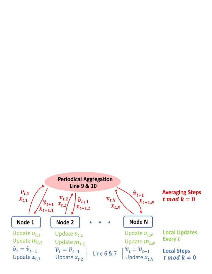
Figure 1: Illustration of the proposed local AMSGrad scheme (Algorithm 3) with shared adaptive learning rate. The local servers employ AMSGrad updates locally, and the global server aggregates the model parameters and second moment $\hat{v}$ every $k$ steps.

Algorithm 3 Local AMSGrad (with N nodes)

1:  Input: learning rate $\alpha$, point $x_{t}$, $m_{t,i}=0,\hat{v}_{0,i}=\epsilon\mathbf{1},\forall i$

2:  $g_{t,i}\leftarrow\nabla f_{i}(x_{t,i})+\xi_{t,i}$

3:  $m_{t,i}=\beta_{1}m_{t-1,i}+(1-\beta_{1})g_{t,i}$

4:  $v_{t,i}=\beta_{2}v_{t-1,i}+(1-\beta_{2})g_{t,i}^{2}$

5:  if $t\mod k\neq 0$ then

6:     $\hat{v}_{t}=\hat{v}_{t-1}$

7:     $x_{t+1,i}\leftarrow x_{t,i}-\alpha\frac{m_{t,i}}{\sqrt{\hat{v}_{t}}}$

8:  else

9:     $\hat{v}_{t}=\max(\frac{1}{N}\sum_{i=1}^{N}v_{t,i},\hat{v}_{t-1})$

10:     $x_{t+1,i}\leftarrow\frac{1}{N}\sum_{j=1}^{N}\left(x_{t,j}-\alpha\frac{m_{t,j}}{\sqrt{\hat{v}_{t}}}\right)$

11:  end if

Compared with Algorithm 2, Algorithm 3 introduces a periodic averaging step for $v_{t,i}$ and updates $\hat{v}_{t}$ at the server side, the same $\hat{v}_{t}$ is used for local updates of different nodes. The intuition behind the design is that, since $v_{t,i}$ can be viewed as second moment estimation of the gradients and the average of $v_{t,i}$ is also an estimation of second moment, we expect the performance of the proposed method to be close to original AMSGrad. Note that this is not the only way to synchronize adaptive learning rate at different nodes, e.g., one can keep $\hat{v}_{t,i}$ locally and use the average of $\hat{v}_{t,i}$ obtained at the previous averaging step as the adaptive learning rate during local updates. With the synchronization of adaptive learning rates, the divergence example in Theorem 4.1 is no longer valid. Nevertheless, the convergence guarantee of the proposed algorithm is still not clear since it uses periodic averaging with adaptive learning rates and momentum. In the next section, we will establish the convergence guarantee of the proposed algorithm.

5 Convergence of Local AMSGrad

In this section, we analyze the convergence behavior of Algorithm 3. The main result is summarized in Theorem 5.1.

Theorem 5.1.

For Algorithm 3, if A1 - A4 are satisfied, define $\overline{x}_{t}=\frac{1}{N}\sum_{i=1}^{N}x_{t,i}$, set $\alpha=\min(\frac{\sqrt{N}}{\sqrt{Td}},\frac{\sqrt{\epsilon}}{4L})$, we have for any $T\geq\frac{16NL^{2}}{\epsilon d}$,

$$\frac{1}{T}\sum_{t=1}^{T}\mathbb{E}\left[\left\|\frac{{\nabla f}(\overline{x}_{t})}{\hat{v}_{t}^{1/4}}\right\|^{2}\right]\leq 8\frac{\sqrt{d}}{\sqrt{TN}}(\mathbb{E}[f(\overline{x}_{1})]-\min_{x}f(x))+8{L}\frac{\sqrt{d}}{\sqrt{TN}}\sigma^{2}\frac{1}{\epsilon}$$

$$+8\frac{d}{T}\frac{\beta_{1}}{1-\beta_{1}}G^{2}\frac{1}{\epsilon^{1/2}}+8\frac{LN}{T^{2}}\frac{\beta_{1}^{2}}{(1-\beta_{1})^{2}}\frac{G^{2}}{\epsilon}$$

$$+8\frac{N}{T}{L}\left(\frac{\beta_{1}^{2}}{(1-\beta_{1})^{2}}+5(k-1)^{2}\right)\frac{G^{2}}{\epsilon^{1.5}}.$$ (1)

From Theorem 5.1, we can analyze the effect of different factors on the convergence rate of Algorithm 3. The first two terms are standard in convergence analysis, which are introduced by initial function value and the variance of the gradient estimator. Note that the $\sqrt{d}$ factor in the two terms is due to the bounded coordinate-wise variance assumption, which makes the total variance of the gradient estimator upper bounded by $d\sigma^{2}$. One can remove the dependency on $d$ on these two terms by assuming bounded total variance. The terms diminishes with $\beta_{1}$ are introduced by the use of momentum in $m_{t,i}$. The most important term for communication efficiency is the term grows with $k$, the number of local updates. This is due to the bias on update directions introduced by local updates. It is clear that this term will not dominate RHS of (5.1) when $k\leq O(\frac{T^{1/4}d^{1/4}}{\sqrt{N}})$. Thus, one can achieve a convergence rate of $O(\sqrt{d}/{\sqrt{TN}})$ with communication rounds sublinear in $T$. This matches the convergence rate of vanilla AMSGrad $O(\sqrt{d}/\sqrt{T})$ proven in Chen et al. (2019a); Zhou et al. (2018). Another aspect which deserves some discussion is the dependency on $\epsilon$. One may expect the RHS to be large when $\epsilon$ is small. However, this is only true when the gradients are also small such that their $L_{\infty}$ norm is in the order of $\epsilon$. All the dependencies on $\epsilon$ appears in lower bounding $\hat{v}_{t}$. With the update rule of $\hat{v}_{t}$, it will quickly become at least the same order as second moment of stochastic gradients, which does not achieve the worst case. Thus, one should expect that when $\epsilon$ is really small, the worst case convergence rate is not achieved in practice. As for the convergence measure, one can easily lower bound LHS of (5.1) by the traditional measure $\frac{1}{T}\sum_{t=1}^{T}\mathbb{E}[\|\nabla f(\bar{x}_{t})\|^{2}]$ using the fact that $\|\hat{v}_{t}\|\leq G^{2}$. To wrap things up, we simplify the convergence rate in Corollary 5.2.

Corollary 5.2.

For Algorithm 3, if A1 - A4 are satisfied, set $k\leq T^{1/4}d^{1/4}/\sqrt{N}$, for $T\geq\max(Nd,\frac{16NL^{2}}{\epsilon d})$ when $\beta_{1}>0$ and for $T\geq\frac{16NL^{2}}{\epsilon d}$ when $\beta_{1}=0$, we have

$$\frac{1}{T}\sum_{t=1}^{T}\mathbb{E}\left[\left\|{{\nabla f}(\overline{x}_{t})}\right\|^{2}\right]\leq O\left(\frac{\sqrt{d}}{\sqrt{TN}}\right).$$

Again, the $\sqrt{d}$ factor is due to the bounded coordinate-wise variance assumption A3, one can easily remove the $d$ dependency by assuming bounded total variance. The proof of Theorem 5.1 can be found in Appendix A.

6 Experiments

We compare the performance of local SGD, local AMSGrad, and naive local AMSGrad on a synthetic Gaussian mixture dataset (Sagun et al., 2017), the letter recogintion dataset (Frey and Slate, 1991) and the standard MNIST dataset. Experiments were conducted using the PaddlePaddle deep learning platform.

6.1 Gaussian mixture dataset (non-i.i.d. case)

In the first experiment, we use the synthetic dataset (Gaussian cluster data) from Sagun et al. (2017). We use 10 isotropic 100 dimensional Gaussian distributions with different mean and same standard deviation to generate the data. The standard deviation of each dimension is 1. The mean of each cluster is generated from an isotropic Gaussian distribution with marginal $N(0,1)$ for each dimension. The labels are the corresponding indices of the cluster from which the data are drawn. The model is a neural network with 2 hidden layers with 50 nodes per layer, and the activation function is ReLU for both layers. The batch size in training is 256. We use $N=5$ workers with each worker containing data from two classes. This assignment of data corresponds to a non-i.i.d. distribution of data on different nodes. The average local period $k$ is set to 10. We perform the learning rate search on a log scale, and increase the learning rate starting from 1e-6 until the algorithm diverges or the performance deteriorates significantly. Specifically, the maximum learning rate is 1 for local SGD and 1e-2 for both local AMSGrad and naive local AMSGrad.

We compare the performance of the algorithms with their best learning rate in Figure 2. It can be seen that local SGD and local AMSGrad perform very similarly. Naive local AMSGrad is worse than the other two algorithms by a small margin.

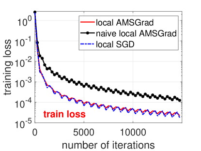
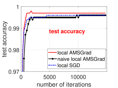
Figure 2: Gaussian mixture dataset: Performance comparison of three different algorithms.

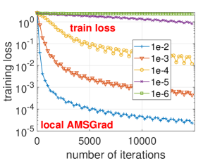
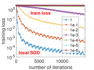
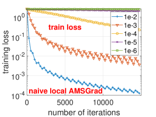
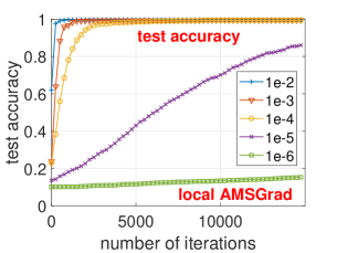
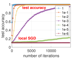
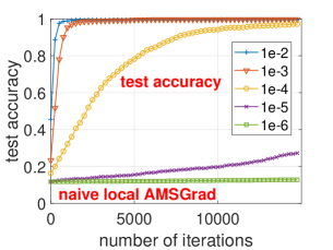
Figure 3: Gaussian mixture dataset: Performance comparison of different stepsizes for three methods.

The performance of different algorithms with different learning rate is shown in Figure 3. It can be seen that all algorithms perform well with suitable learning rate. From these results, it seems that local AMSGrad do not have clear advantages over other algorithms. In particular, naive local AMSGrad performs not bad albeit it lacks convergence guarantee. We conjecture that this is due to that such a simple dataset cannot make the adaptive learning rate on different nodes differ significantly. In the next sets of experiments, we use more complicated real-world datasets to test the performance of different algorithms.

6.2 MNIST dataset (non-i.i.d. case)

In this section, we compare the algorithms on training a convolutional neural network (CNN) on MNIST. Similar to last set of experiments, we perform learning rate search starting from 1e-6 until the algorithm diverges or deteriorates significantly. The average period $k$ is set to 10. We set $\epsilon$ to be 1e-4 for both Adam and AMSGrad. The data is distributed on 5 nodes and each node contains data from two classes, and there is no overlap on labels between different nodes. We expect such an allocation of data can creates a highly non-i.i.d. data distribution, leading to significantly different adaptive learning rates on different nodes. The neural network in the experiments consists of 3 convolution+pooling layers with ReLu activation, followed by a 10 nodes fully connected layer with softmax activation. The first convolution+pooling layer has 20 5x5 filters followed by 2x2 max pooling with stride 2. The second and third convolution+polling layer has 50 filters with other parameters being the same as the first layer.

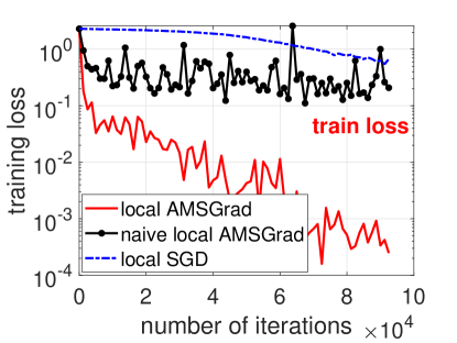
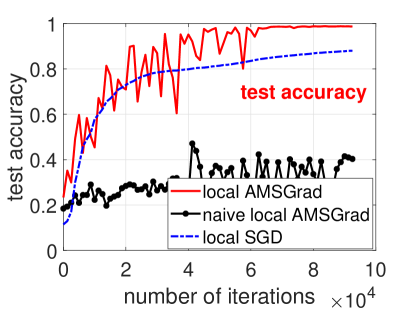
Figure 4: MNIST dataset: Performance comparison of three different algorithms.

Figure 4 shows the training and testing performance of different algorithms. Specifically, 1e-3 is chosen for local AMSGrad and naive local AMSGrad while 1e-4 is chosen for local SGD. It can be seen that local AMSGrad outperforms local SGD by a large margin.

The performance of algorithms with different learning rate is shown in Figure 5. We observe that naive local AMSGrad has very poor performance with all learning rate choices, and local AMSGrad tend to perform better than local SGD on average. The slow convergence of local SGD is also observed in McMahan et al. (2017) when the data distribution is non-i.i.d. While the sampling on nodes in McMahan et al. (2017) may somehow reduce the influence of non-i.i.d. data, the convergence speed of local SGD is significantly impacted by the non-i.i.d. distribution in our experiment since we always use all nodes for parameter update.

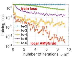
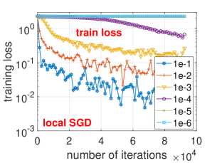
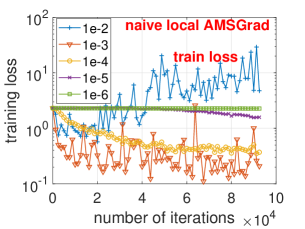
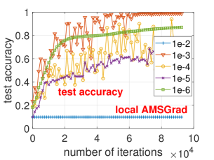
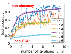
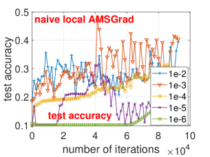
Figure 5: MNIST dataset: Performance comparison of different stepsizes for three methods.

6.3 Letter recognition dataset (i.i.d. case)

    

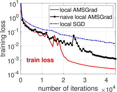
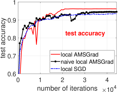
Figure 6: Letter recognition dataset: Performance comparison of three different algorithms.

In this section, we use the letter recognition dataset Frey and Slate (1991) to test the performance of different algorithms. We train a fully connected neural network with two hidden layers on the dataset. The first hidden layer has 300 nodes and the second layer has 200 nodes, both of which use ReLU as activation. The learning rate search strategy and other parameter settings are the same as the MNIST experiments. Different from the previous two sets of experiments, the data on the 5 workers are randomly assigned. This corresponds to an i.i.d. data distribution. Thus, all algorithms are expected to work well in this set of experiments. The performance comparison of algorithms with their best learning rate is provided in Figure 6. We can see that all algorithms achieve over 90% accuracy and local AMSGrad again performs the best, with 2% higher test accuracy than local SGD. In this case, naive local AMSGrad is also better than local SGD. Thus, when data distribution is i.i.d., it might be okay to use the naive version of local AMSGrad in practice, considering that it involves even less communication. The performance of algorithms with different learning rate is shown in Figure 7, which shows that all algorithms perform quite stable, while the two adaptive gradient methods still outperform local SGD in general.

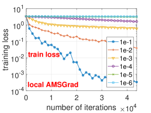
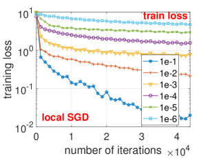
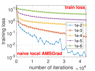
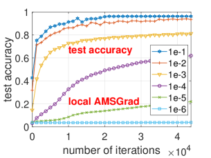
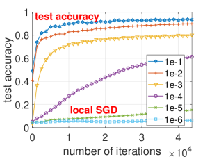
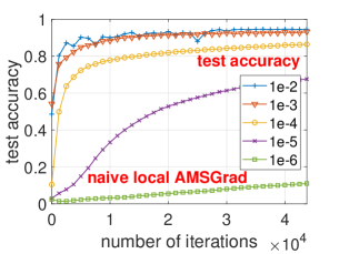
Figure 7: Letter recognition dataset: Performance comparison of different stepsizes for three methods.

7 Conclusion

In this paper, we study how to design adaptive gradient methods for federated learning by utilizing periodic model averaging. We first construct counter examples to illustrate how a naive combination of adaptive gradient methods and periodic model averaging can fail to converge. Then, by utilizing the insights from the study of non-convergence, we propose an adaptive gradient method local AMSGrad in the setting of federated learning with proved convergence guarantee.    Local AMSGrad enjoys the sublinear communication cost of periodic model averaging as well as the superb empirical performance of adaptive gradient methods. Experiments show that local AMSGrad can often significantly outperform both the local SGD and a naive design of local adaptive gradient methods, especially when the dada distribution on different nodes is non-i.i.d.

Appendix

Appendix A Proof of Theorem 5.1

To prove the convergence of local AMSGrad, we first define an auxiliary sequence of iterates

$$\overline{z}_{t}=\overline{x}_{t}+\frac{\beta_{1}}{1-\beta_{1}}(\overline{x}_{t}-\overline{x}_{t-1}).$$ (2)

where $\overline{x}_{t}=\frac{1}{N}\sum_{i=1}^{N}x_{t,i}$ and we define $x_{0}\triangleq x_{1}$.

We have the following property for the new sequence $\overline{z}_{t}$.

Lemma A.1.

For $\overline{z}_{t}$ defined in (2),

$$\overline{z}_{t+1}-\overline{z}_{t}=\alpha\frac{\beta_{1}}{1-\beta_{1}}\left(\frac{1}{\sqrt{\hat{v}_{t-1}}}-\frac{1}{\sqrt{\hat{v}_{t}}}\right)\odot\overline{m}_{t-1}-\alpha\frac{\overline{g}_{t}}{\sqrt{\hat{v}_{t}}}.$$ (3)

where $\overline{m}_{t-1}=\frac{1}{N}\sum_{i=1}^{N}m_{t-1,i}$ and $\overline{g}_{t}=\frac{1}{N}\sum_{i=1}^{N}g_{t,i}$.

Proof: We have

$$\overline{z}_{t+1}-\overline{z}_{t} =\overline{x}_{t+1}+\frac{\beta_{1}}{1-\beta_{1}}(\overline{x}_{t+1}-\overline{x}_{t})-\overline{x}_{t}-\frac{\beta_{1}}{1-\beta_{1}}(\overline{x}_{t}-\overline{x}_{t-1})$$

$$=\frac{1}{1-\beta_{1}}(\overline{x}_{t+1}-\overline{x}_{t})-\frac{\beta_{1}}{1-\beta_{1}}(\overline{x}_{t}-\overline{x}_{t-1})$$

$$=\frac{\alpha}{1-\beta_{1}}\frac{\overline{m}_{t}}{\sqrt{\hat{v}_{t}}}-\frac{\alpha\beta_{1}}{1-\beta_{1}}\frac{\overline{m}_{t-1}}{\sqrt{\hat{v}_{t-1}}}.$$

By the updating rule of Algorithm 3, we have $\overline{m}_{t}=\beta_{1}\overline{m}_{t-1}+(1-\beta_{1})\overline{g}_{t}$. Thus,

$$\overline{z}_{t+1}-\overline{z}_{t} =\frac{\alpha\beta_{1}}{1-\beta_{1}}\left(\frac{1}{\sqrt{\hat{v}_{t}}}-\frac{1}{\sqrt{\hat{v}_{t-1}}}\right)\odot\overline{m}_{t-1}+\alpha\frac{\overline{g}_{t}}{\sqrt{\hat{v}_{t}}},$$

which completes the proof. $\square$

In what follows, we use the auxiliary sequence $\bar{z}_{t}$ in Lemma A.1 to prove convergence of the algorithm.

By Lipschitz continuity, we have

$$f(\overline{z}_{t+1})\leq f(\overline{z}_{t})+\langle\nabla f(\overline{z}_{t}),\overline{z}_{t+1}-\overline{z}_{t}\rangle+\frac{L}{2}\|\overline{z}_{t+1}-\overline{z}_{t}\|^{2},$$

and thus

$$-\mathbb{E}[\langle\nabla f(\overline{z}_{t}),\overline{z}_{t+1}-\overline{z}_{t}\rangle]\leq \mathbb{E}[f(\overline{z}_{t})]-\mathbb{E}[f(\overline{z}_{t+1})]+\frac{L}{2}\mathbb{E}[\|\overline{z}_{t+1}-\overline{z}_{t}\|^{2}].$$ (4)

where the expectation is taken over all the randomness of stochastic gradients until iteration $t$.

It remains to upper bound the second-order term on RHS of (4) and characterize the effective descent in the first order term (LHS of (4)). We first characterize the effective descent.

By (3), we can write the first-order term as

$$\langle\nabla f(\overline{z}_{t}),\overline{z}_{t+1}-\overline{z}_{t}\rangle= \alpha\langle\nabla f(z_{t}),\frac{\beta_{1}}{1-\beta_{1}}\left(\frac{1}{\sqrt{\hat{v}_{t-1}}}-\frac{1}{\sqrt{\hat{v}_{t}}}\right)\odot\overline{m}_{t-1}$$

$$- \alpha\langle\nabla f(z_{t}),\frac{\overline{g}_{t}}{\sqrt{\hat{v}_{t}}}\rangle.$$ (5)

Since $\hat{v}_{t}$ is independent of $\overline{g}_{t}$ and $\mathbb{E}[g_{t,i}]=\nabla f_{i}(x_{t,i})$, taking expectation on both sides of (A) yields

$$\mathbb{E}\left[\langle\nabla f(\overline{z}_{t}),\overline{z}_{t+1}-\overline{z}_{t}\rangle\right]= \alpha\mathbb{E}\left[\langle\nabla f(z_{t}),\frac{\beta_{1}}{1-\beta_{1}}\left(\frac{1}{\sqrt{\hat{v}_{t-1}}}-\frac{1}{\sqrt{\hat{v}_{t}}}\right)\odot\overline{m}_{t-1}\right]$$

$$- \alpha\mathbb{E}\left[\langle\nabla f(z_{t}),\frac{\overline{\nabla f}(x_{t})}{\sqrt{\hat{v}_{t}}}\rangle\right],$$

where $\overline{\nabla f}(x_{t})=\frac{1}{N}\sum_{i=1}^{N}\nabla f_{i}(x_{t,i})$.

Using the fact $\langle a,b\rangle=\frac{1}{2}(\|a-b\|^{2}-\|a\|^{2}-\|b\|^{2})$, we have

$$\langle\nabla f(\overline{z}_{t}),\frac{\overline{\nabla f}(x_{t})}{\sqrt{\hat{v}_{t}}}\rangle= \frac{1}{2}\left\|\frac{\nabla f(\overline{z}_{t})}{\hat{v}_{t}^{1/4}}\right\|^{2}+\frac{1}{2}\left\|\frac{\overline{\nabla f}(x_{t})}{\hat{v}_{t}^{1/4}}\right\|^{2}-\left\|\frac{\nabla f(\overline{z}_{t})-\overline{\nabla f}(x_{t})}{\hat{v}_{t}^{1/4}}\right\|^{2},$$ (6)

where the first two quantities on RHS of (6) will contribute to the descent of objective in a single optimization step, while the last term is the possible ascent introduced by the bias on the stochastic gradients. The bound of the last term is given by Lemma A.2.

Lemma A.2.

For Algorithm 3, we have

$$\left\|\frac{\nabla f(\overline{z}_{t})-\overline{\nabla f}(x_{t})}{\hat{v}_{t}^{1/4}}\right\|^{2}\leq \frac{L}{\min_{j}(\hat{v}_{t}^{1/2})_{j}}\left(2\frac{\beta_{1}^{2}}{(1-\beta_{1})^{2}}+8(k-1)^{2}\right)\alpha^{2}d\frac{G^{2}}{\epsilon}.$$ (7)

Proof: First, we have

$$\left\|\frac{\nabla f(\overline{z}_{t})-\overline{\nabla f}(x_{t})}{\hat{v}_{t}^{1/4}}\right\|^{2}$$

$$= \left\|\frac{\frac{1}{N}\sum_{i=1}^{N}(\nabla f_{i}(\overline{z}_{t})-{\nabla f_{i}}(x_{t,i}))}{\hat{v}_{t}^{1/4}}\right\|^{2}$$

$$\leq \frac{1}{N}\sum_{i=1}^{N}\left\|\frac{\nabla f_{i}(\overline{z}_{t})-{\nabla f_{i}}(x_{t,i})}{\hat{v}_{t}^{1/4}}\right\|^{2}$$

$$\leq \frac{1}{N}\sum_{i=1}^{N}2\left(\left\|\frac{\nabla f_{i}(\overline{z}_{t})-\nabla f_{i}(\overline{x}_{t})}{\hat{v}_{t}^{1/4}}\right\|^{2}+\left\|\frac{\nabla f_{i}(\overline{x}_{t})-{\nabla f_{i}}(x_{t,i})}{\hat{v}_{t}^{1/4}}\right\|^{2}\right),$$ (8)

where the last inequality is due to Cauchy-Schwartz.

Using Lipschitz property (Assumption A1) of $\nabla f_{i}$, we can further bound the differences of gradients on RHS of (8) by

$$\frac{2}{N}\sum_{i=1}^{N}\left\|\frac{\nabla f_{i}(\overline{z}_{t})-\nabla f_{i}(\overline{x}_{t})}{\hat{v}_{t}^{1/4}}\right\|^{2}\leq\frac{2}{N}\sum_{i=1}^{N}\frac{\left\|{\nabla f_{i}(\overline{z}_{t})-\nabla f_{i}(\overline{x}_{t})}{}\right\|^{2}}{\min_{j}(\hat{v}_{t}^{1/2})_{j}}\leq\frac{2}{N}\sum_{i=1}^{N}\frac{L\|\overline{z}_{t}-\overline{x}_{t}\|^{2}}{\min_{j}(\hat{v}_{t}^{1/2})_{j}}.$$ (9)

Similarly, we have

$$\frac{2}{N}\sum_{i=1}^{N}\left\|\frac{\nabla f_{i}(\overline{x}_{t})-{\nabla f_{i}}(x_{t,i})}{\hat{v}_{t}^{1/4}}\right\|^{2}\leq\frac{2}{N}\sum_{i=1}^{N}\frac{L\|\overline{x}_{t}-x_{t,i}\|^{2}}{\min_{j}(\hat{v}_{t}^{1/2})_{j}}.$$ (10)

It remains to bound $\|\overline{z}_{t}-\overline{x}_{t}\|^{2}$ and $\|\overline{x}_{t}-x_{t,i}\|^{2}$ using the update rule of $x$ and $z$. For the difference between $\overline{z}_{t}$ and $\overline{x}_{t}$, we have

$$\sum_{i=1}^{N}\left\|{\overline{z}_{t}-\overline{x}_{t}}{}\right\|^{2}= \frac{\beta_{1}^{2}}{(1-\beta_{1})^{2}}\sum_{i=1}^{N}\left\|{\overline{x}_{t}-\overline{x}_{t-1}}{}\right\|^{2}$$

$$= \frac{\beta_{1}^{2}}{(1-\beta_{1})^{2}}\alpha^{2}N\left\|\frac{\overline{m}_{t-1}}{\sqrt{\hat{v}_{t-1}}}\right\|^{2}$$

$$\leq \frac{\beta_{1}^{2}}{(1-\beta_{1})^{2}}\alpha^{2}Nd\frac{G^{2}}{\epsilon},$$ (11)

where $\overline{m}_{t}=\frac{1}{N}\sum_{i=1}^{N}m_{t,i}$. For the second term containing the consensus error $\overline{x}_{t}-x_{t,i}$, we have

$$\sum_{i=1}^{N}\left\|{\overline{x}_{t}-x_{t,i}}{}\right\|^{2}\leq 4N(k-1)^{2}\alpha^{2}d\frac{G^{2}}{\epsilon}$$ (12)

by Lemma A.3, which is presented next.

Lemma A.3.

For iterates produced by Algorithm 3, we have

$$\left\|{\overline{x}_{t}-x_{t,i}}{}\right\|^{2}\leq 4(k-1)^{2}\alpha^{2}d\frac{G^{2}}{\epsilon},\vspace{0.2in}\forall i\in[N].$$

Proof: Let $\lfloor t\rfloor_{k}$ be the largest multiple of $k$ that is less than $t$. By the updating rule of Algorithm 3, we have

$$x_{t,i}=\overline{x}_{\lfloor t\rfloor_{k}+1}-\alpha\sum_{l=\lfloor t\rfloor_{k}+1}^{t-1}\frac{m_{l,i}}{\sqrt{\hat{v}_{l}}},$$

since $x_{t,i}^{\prime}s$ are averaged on steps $ck+1,c\in\mathbb{N}_{0}$. Thus, we have

$$\left\|{\overline{x}_{t}-x_{t,i}}{}\right\|^{2}= \alpha^{2}\left\|\sum_{l=\lfloor t\rfloor_{k}+1}^{t-1}\left(\frac{m_{l,i}}{\sqrt{\hat{v}_{l}}}-\frac{1}{N}\sum_{o=1}^{N}\frac{m_{l,o}}{\sqrt{\hat{v}_{o}}}\right)\right\|^{2}$$

$$\leq 4N(k-1)^{2}\alpha^{2}d\frac{G^{2}}{\epsilon},$$

because $(t-1)-(\lfloor t\rfloor_{k}+1)+1\leq k-1$, and $(\hat{v}_{o})_{j}\geq\epsilon,\forall j\in[d],o\in[N]$, and $\|m_{t,o}\|_{\infty}\leq G,\forall t,o$. $\square$

Combining (8), (9), (10), (A) and (12), we obtain

$$\left\|\frac{\nabla f(\overline{z}_{t})-\overline{\nabla f}(x_{t})}{\hat{v}_{t}^{1/4}}\right\|^{2}\leq \frac{L}{\min_{j}(\hat{v}_{t}^{1/2})_{j}}\left(2\frac{\beta_{1}^{2}}{(1-\beta_{1})^{2}}+8(k-1)^{2}\right)\alpha^{2}d\frac{G^{2}}{\epsilon}.$$

which is the desired bound. This completes the proof. $\square$

Therefore, by (6) and (7), we have

$$-\langle\nabla f(\overline{z}_{t}),\frac{\overline{\nabla f}(x_{t})}{\sqrt{\hat{v}_{t}}}\rangle\leq -\frac{1}{2}\left\|\frac{\nabla f(\overline{z}_{t})}{\hat{v}_{t}^{1/4}}\right\|^{2}-\frac{1}{2}\left\|\frac{\overline{\nabla f}(x_{t})}{\hat{v}_{t}^{1/4}}\right\|^{2}+\alpha^{2}\frac{L}{\min_{j}(\hat{v}_{t}^{1/2})_{j}}\left(\frac{\beta_{1}^{2}}{(1-\beta_{1})^{2}}+4(k-1)^{2}\right)d\frac{G^{2}}{\epsilon}.$$ (13)

Substituting (13) into (A) and (4) yields

$$\alpha\mathbb{E}\left[\frac{1}{2}\left\|\frac{\nabla f(\overline{z}_{t})}{\hat{v}_{t}^{1/4}}\right\|^{2}+\frac{1}{2}\left\|\frac{\overline{\nabla f}(x_{t})}{\hat{v}_{t}^{1/4}}\right\|^{2}\right]$$

$$\leq \mathbb{E}[f(\overline{z}_{t})]-\mathbb{E}[f(\overline{z}_{t+1})]+\frac{L}{2}\mathbb{E}[\|\overline{z}_{t+1}-\overline{z}_{t}\|^{2}]$$

$$\hskip 36.135pt+\alpha\mathbb{E}\left[\langle\nabla f(\overline{z}_{t}),\frac{\beta_{1}}{1-\beta_{1}}\left(\frac{1}{\sqrt{\hat{v}_{t-1}}}-\frac{1}{\sqrt{\hat{v}_{t}}}\right)\odot\overline{m}_{t-1}\right]$$

$$\hskip 36.135pt+\alpha^{3}\mathbb{E}\left[\frac{L}{\min_{j}(\hat{v}_{t}^{1/2})_{j}}\left(\frac{\beta_{1}^{2}}{(1-\beta_{1})^{2}}+4(k-1)^{2}\right)d\frac{G^{2}}{\epsilon}\right].$$

Summing over $t$ from 1 to $T$ and divide both sides by $T\alpha$, we get

$$\frac{1}{T}\sum_{t=1}^{T}\mathbb{E}\left[\frac{1}{2}\left\|\frac{\nabla f(\overline{z}_{t})}{\hat{v}_{t}^{1/4}}\right\|^{2}+\frac{1}{2}\left\|\frac{\overline{\nabla f}(x_{t})}{\hat{v}_{t}^{1/4}}\right\|^{2}\right]$$

$$\leq \frac{1}{T\alpha}(\mathbb{E}[f(\overline{z}_{1})]-\mathbb{E}[f(\overline{z}_{T+1})])+\frac{L}{2}\frac{1}{T\alpha}\underbrace{\sum_{t=1}^{T}\mathbb{E}[\|\overline{z}_{t+1}-\overline{z}_{t}\|^{2}]}_{T_{1}}$$

$$+\frac{1}{T}\underbrace{\sum_{t=1}^{T}\mathbb{E}\left[\left\langle\nabla f(\overline{z}_{t}),\frac{\beta_{1}}{1-\beta_{1}}\left(\frac{1}{\sqrt{\hat{v}_{t-1}}}-\frac{1}{\sqrt{\hat{v}_{t}}}\right)\odot\overline{m}_{t-1}\right\rangle\right]}_{T_{2}}$$

$$+\alpha^{2}\frac{1}{T}\sum_{t=1}^{T}\mathbb{E}\left[\frac{L}{\min_{j}(\hat{v}_{t}^{1/2})_{j}}\left(\frac{\beta_{1}^{2}}{(1-\beta_{1})^{2}}+4(k-1)^{2}\right)d\frac{G^{2}}{\epsilon}\right].$$ (14)

What remains is to bounded $T_{1}$ and $T_{2}$.

Lemma A.4.

We have

$$T_{1}\leq 2\alpha^{2}\sum_{t=1}^{T}\mathbb{E}\left[\left\|\frac{\overline{\nabla f}(x_{t})}{\sqrt{\hat{v}_{t}}}\right\|^{2}+\frac{1}{N}\sigma^{2}\left\|\frac{1}{\sqrt{\hat{v}_{t}}}\right\|^{2}\right]+2\alpha^{2}\frac{\beta_{1}^{2}}{(1-\beta_{1})^{2}}G^{2}\frac{d}{\epsilon}.$$

Proof: By (3), we know that

$$\|\overline{z}_{t+1}-\overline{z}_{t}\|^{2}$$

$$= \alpha^{2}\left\|\frac{\beta_{1}}{1-\beta_{1}}\left(\frac{1}{\sqrt{\hat{v}_{t-1}}}-\frac{1}{\sqrt{\hat{v}_{t}}}\right)\odot\overline{m}_{t-1}-\alpha\frac{\overline{g}_{t}}{\sqrt{\hat{v}_{t}}}\right\|^{2}$$

$$\leq 2\alpha^{2}\left(\left\|\frac{\beta_{1}}{1-\beta_{1}}\left(\frac{1}{\sqrt{\hat{v}_{t-1}}}-\frac{1}{\sqrt{\hat{v}_{t}}}\right)\odot\overline{m}_{t-1}\right\|^{2}+\left\|\frac{\overline{g}_{t}}{\sqrt{\hat{v}_{t}}}\right\|^{2}\right).$$

In addition, conditioned on all randomness in $\hat{v}_{t}$ (gradients from iteration $1$ until $t-1$), we have

$$\mathbb{E}\left[\left\|\frac{\overline{g}_{t}}{\sqrt{\hat{v}_{t}}}\right\|^{2}\right]= \mathbb{E}\left[\left\|\frac{1}{N}\sum_{i=1}^{N}\frac{g_{t,i}}{\sqrt{\hat{v}_{t}}}\right\|^{2}\right]=\frac{1}{N^{2}}\mathbb{E}\left[\sum_{j=1}^{N}\sum_{i=1}^{N}\left\langle\frac{g_{t,i}}{\sqrt{\hat{v}_{t}}},\frac{g_{t,j}}{\sqrt{\hat{v}_{t}}}\right\rangle\right]$$

$$\stackrel{{\scriptstyle(a)}}{{=}} \frac{1}{N^{2}}\mathbb{E}\left[\sum_{j=1}^{N}\sum_{i=1}^{N}\left\langle\frac{\nabla f_{i}(x_{t,i})+\xi_{t,i}}{\sqrt{\hat{v}_{t}}},\frac{\nabla f_{j}(x_{t,j})+\xi_{t,j}}{\sqrt{\hat{v}_{t}}}\right\rangle\right]$$

$$\stackrel{{\scriptstyle(b)}}{{=}} \frac{1}{N^{2}}\left\|\frac{\sum_{i=1}^{N}\nabla f_{i}(x_{t,i})}{\sqrt{\hat{v}_{t}}}\right\|^{2}+\frac{1}{N^{2}}\sum_{i=1}^{N}\mathbb{E}\left[\left\|\frac{\xi_{t,i}}{\sqrt{\hat{v}_{t}}}\right\|^{2}\right]$$

$$\stackrel{{\scriptstyle(c)}}{{\leq}} \left\|\frac{\overline{\nabla f}(x_{t})}{\sqrt{\hat{v}_{t}}}\right\|^{2}+\frac{1}{N}\sigma^{2}\left\|\frac{1}{\sqrt{\hat{v}_{t}}}\right\|^{2},$$

where $(a)$ is a reparameterization of the noises on gradients, $(b)$ is due to the assumption that all elements of $\xi_{t,i}$’s are independent of each other and $\mathbb{E}[(\xi_{t,i})_{j}]=0,\forall j\in[d]$, and (c) is by the assumption that $E[(\xi_{t,i})_{j}^{2}]\leq\sigma$ and the fact that $\hat{v}_{t}$ and $x_{t,i}$ are both fixed given all gradients before iteration $t$. Furthermore, we have

$$\left\|\frac{\beta_{1}}{1-\beta_{1}}\left(\frac{1}{\sqrt{\hat{v}_{t-1}}}-\frac{1}{\sqrt{\hat{v}_{t}}}\right)\odot\overline{m}_{t-1}\right\|^{2}$$

$$\leq \frac{\beta_{1}^{2}}{(1-\beta_{1})^{2}}G^{2}\sum_{j=1}^{d}\left(\frac{1}{\sqrt{(\hat{v}_{t-1})_{j}}}-\frac{1}{\sqrt{(\hat{v}_{t})_{j}}}\right)^{2}$$

$$\leq \frac{\beta_{1}^{2}}{(1-\beta_{1})^{2}}G^{2}\frac{1}{\epsilon^{1/2}}\sum_{j=1}^{d}\left|\frac{1}{\sqrt{(\hat{v}_{t-1})_{j}}}-\frac{1}{\sqrt{(\hat{v}_{t})_{j}}},\right|$$

and thus

$$\sum_{t=1}^{T}\left\|\frac{\beta_{1}}{1-\beta_{1}}\left(\frac{1}{\sqrt{\hat{v}_{t-1}}}-\frac{1}{\sqrt{\hat{v}_{t}}}\right)\odot\overline{m}_{t-1}\right\|^{2}$$

$$\leq \sum_{t=1}^{T}\frac{\beta_{1}^{2}}{(1-\beta_{1})^{2}}G^{2}\frac{1}{\epsilon^{1/2}}\sum_{j=1}^{d}\left|\frac{1}{\sqrt{(\hat{v}_{t-1})_{j}}}-\frac{1}{\sqrt{(\hat{v}_{t})_{j}}}\right|$$

$$\leq \frac{\beta_{1}^{2}}{(1-\beta_{1})^{2}}G^{2}\frac{1}{\epsilon^{1/2}}\sum_{j=1}^{d}\left|\frac{1}{\sqrt{(\hat{v}_{0})_{j}}}\right|=\frac{\beta_{1}^{2}}{(1-\beta_{1})^{2}}G^{2}\frac{1}{\epsilon}d,$$

where the last inequality is due to non-decreasing property of $\hat{v}_{t}$.

Combining all above, we obtain

$$T_{1}\leq 2\alpha^{2}\sum_{t=1}^{T}\mathbb{E}\left[\left\|\frac{\overline{\nabla f}(x_{t})}{\sqrt{\hat{v}_{t}}}\right\|^{2}+\frac{1}{N}\sigma^{2}\left\|\frac{1}{\sqrt{\hat{v}_{t}}}\right\|^{2}\right]+2\alpha^{2}\frac{\beta_{1}^{2}}{(1-\beta_{1})^{2}}G^{2}\frac{d}{\epsilon}.$$

This completes the proof. $\square$

Now we can examine $T_{2}$. We have

$$T_{2}= \sum_{t=1}^{T}\mathbb{E}\left[\left\langle\nabla f(\overline{z}_{t}),\frac{\beta_{1}}{1-\beta_{1}}\left(\frac{1}{\sqrt{\hat{v}_{t-1}}}-\frac{1}{\sqrt{\hat{v}_{t}}}\right)\odot\overline{m}_{t-1}\right\rangle\right]$$

$$\leq \mathbb{E}\left[\sum_{t=1}^{T}\frac{\beta_{1}}{1-\beta_{1}}G^{2}\sum_{j=1}^{d}\left|\frac{1}{\sqrt{(\hat{v}_{t-1})_{j}}}-\frac{1}{\sqrt{(\hat{v}_{t})_{j}}}\right|\right]$$

$$\leq \mathbb{E}\left[\frac{\beta_{1}}{1-\beta_{1}}G^{2}\sum_{j=1}^{d}\left|\frac{1}{\sqrt{(\hat{v}_{0})_{j}}}\right|\right]=\frac{\beta_{1}}{1-\beta_{1}}G^{2}d\frac{1}{\epsilon^{1/2}},$$

where the second inequality is because $\hat{v}_{t}$ is non-decreasing.

Substituting the bounds on $T_{1}$ and $T_{2}$ into (A), we obtain

$$\frac{1}{T}\sum_{t=1}^{T}\mathbb{E}\left[\frac{1}{2}\left\|\frac{\nabla f(\overline{z}_{t})}{\hat{v}_{t}^{1/4}}\right\|^{2}+\frac{1}{2}\left\|\frac{\overline{\nabla f}(x_{t})}{\hat{v}_{t}^{1/4}}\right\|^{2}\right]$$

$$\leq \frac{1}{T\alpha}(\mathbb{E}[f(\overline{z}_{1})]-\mathbb{E}[f(\overline{z}_{T+1})])$$

$$+\frac{L}{T}\alpha\sum_{t=1}^{T}\mathbb{E}\left[\left\|\frac{\overline{\nabla f}(x_{t})}{\sqrt{\hat{v}_{t}}}\right\|^{2}+\frac{1}{N}\sigma^{2}\left\|\frac{1}{\sqrt{\hat{v}_{t}}}\right\|^{2}\right]$$

$$+\frac{1}{T}\frac{\beta_{1}}{1-\beta_{1}}G^{2}d\frac{1}{\epsilon^{1/2}}+\frac{L}{T}\alpha^{2}\frac{\beta_{1}^{2}}{(1-\beta_{1})^{2}}G^{2}\frac{d}{\epsilon}$$

$$+\alpha^{2}\frac{1}{T}\sum_{t=1}^{T}\mathbb{E}\left[\frac{L}{\min_{j}(\hat{v}_{t}^{1/2})_{j}}\left(\frac{\beta_{1}^{2}}{(1-\beta_{1})^{2}}+4(k-1)^{2}\right)d\frac{G^{2}}{\epsilon}\right].$$ (15)

Further, by choosing $\alpha=\min(\frac{\sqrt{N}}{\sqrt{Td}},\frac{\sqrt{\epsilon}}{4L})$, we have

$${L}\frac{1}{T}\alpha\sum_{t=1}^{T}\mathbb{E}\left[\left\|\frac{\overline{\nabla f}(x_{t})}{\sqrt{\hat{v}_{t}}}\right\|^{2}\right]\leq{L}\frac{1}{T}\alpha\sum_{t=1}^{T}\mathbb{E}\left[\frac{1}{\sqrt{\epsilon}}\left\|\frac{\overline{\nabla f}(x_{t})}{{\hat{v}_{t}^{1/4}}}\right\|^{2}\right]\frac{1}{4}\frac{1}{T}\sum_{t=1}^{T}\mathbb{E}\left[\left\|\frac{\overline{\nabla f}(x_{t})}{{\hat{v}_{t}^{1/4}}}\right\|^{2}\right].$$ (16)

Thus, from (15) and (16), we obtain

$$\frac{1}{T}\sum_{t=1}^{T}\mathbb{E}\left[\frac{1}{2}\left\|\frac{\nabla f(\overline{z}_{t})}{\hat{v}_{t}^{1/4}}\right\|^{2}+\frac{1}{4}\left\|\frac{\overline{\nabla f}(x_{t})}{\hat{v}_{t}^{1/4}}\right\|^{2}\right]$$

$$\leq \frac{1}{T\alpha}(\mathbb{E}[f(\overline{z}_{1})]-\mathbb{E}[f(\overline{z}_{T+1})])+{L}\frac{\sqrt{d}}{\sqrt{TN}}\sigma^{2}\frac{1}{\epsilon}$$

$$+\frac{1}{T}\frac{\beta_{1}}{1-\beta_{1}}G^{2}d\frac{1}{\epsilon^{1/2}}+\frac{LN}{T^{2}}\frac{\beta_{1}^{2}}{(1-\beta_{1})^{2}}\frac{G^{2}}{\epsilon}$$

$$+\frac{N}{T}{L}\left(\frac{\beta_{1}^{2}}{(1-\beta_{1})^{2}}+4(k-1)^{2}\right)\frac{G^{2}}{\epsilon^{1.5}},$$

and when $T\geq\frac{16NL^{2}}{\epsilon d}$, we have

$$\frac{1}{T}\sum_{t=1}^{T}\mathbb{E}\left[\frac{1}{2}\left\|\frac{\nabla f(\overline{z}_{t})}{\hat{v}_{t}^{1/4}}\right\|^{2}+\frac{1}{4}\left\|\frac{\overline{\nabla f}(x_{t})}{\hat{v}_{t}^{1/4}}\right\|^{2}\right]$$

$$\leq \frac{\sqrt{d}}{\sqrt{TN}}(\mathbb{E}[f(\overline{z}_{1})]-\mathbb{E}[f(\overline{z}_{T+1})])+{L}\frac{\sqrt{d}}{\sqrt{TN}}\sigma^{2}\frac{1}{\epsilon}$$

$$+\frac{d}{T}\frac{\beta_{1}}{1-\beta_{1}}G^{2}\frac{1}{\epsilon^{1/2}}+\frac{LN}{T^{2}}\frac{\beta_{1}^{2}}{(1-\beta_{1})^{2}}\frac{G^{2}}{\epsilon}$$

$$+\frac{N}{T}{L}\left(\frac{\beta_{1}^{2}}{(1-\beta_{1})^{2}}+4(k-1)^{2}\right)\frac{G^{2}}{\epsilon^{1.5}}.$$ (17)

At this point, we have obtained the $O(\frac{\sqrt{d}}{\sqrt{TN}})$ convergence rate (when $T$ is sufficiently large), which matches the convergence rate of SGD. One remaining item is to convert the convergence measure to the norm of gradients of $f$. We do this by the following Lemma.

Lemma A.5.

For Algorithm 3, we have

$$\left\|\frac{\overline{\nabla f}(x_{t})}{\hat{v}_{t}^{1/4}}\right\|^{2}\geq\frac{1}{2}\left\|\frac{{\nabla f}(\overline{x}_{t})}{\hat{v}_{t}^{1/4}}\right\|^{2}-4L(k-1)^{2}\alpha^{2}d\frac{G^{2}}{\epsilon^{1.5}}.$$

Proof: We have

$$\left\|\frac{\overline{\nabla f}(x_{t})}{\hat{v}_{t}^{1/4}}\right\|^{2}\geq \frac{1}{2}\left\|\frac{{\nabla f}(\overline{x}_{t})}{\hat{v}_{t}^{1/4}}\right\|^{2}-\left\|\frac{\overline{\nabla f}(x_{t})-{\nabla f}(\overline{x}_{t})}{\hat{v}_{t}^{1/4}}\right\|^{2}$$

$$\geq \frac{1}{2}\left\|\frac{{\nabla f}(\overline{x}_{t})}{\hat{v}_{t}^{1/4}}\right\|^{2}-\frac{1}{N}\sum_{i=1}^{N}\left\|\frac{{\nabla f_{i}}(x_{t,i})-{\nabla f_{i}}(\overline{x}_{t})}{\hat{v}_{t}^{1/4}}\right\|^{2}$$

$$\geq \frac{1}{2}\left\|\frac{{\nabla f}(\overline{x}_{t})}{\hat{v}_{t}^{1/4}}\right\|^{2}-4L(k-1)^{2}\alpha^{2}d\frac{G^{2}}{\epsilon^{1.5}},$$

where the first inequality is due to Cauchy-Schwartz, the second inequality is due to Jensen’s inequality, and the last inequality is due to Lemma A.3 and L-smoothness of $f_{i}$ (A1). $\square$

We can then transform (17) into

$$\frac{1}{T}\sum_{t=1}^{T}\mathbb{E}\left[\frac{1}{8}\left\|\frac{{\nabla f}(\overline{x}_{t})}{\hat{v}_{t}^{1/4}}\right\|^{2}\right]\leq \frac{\sqrt{d}}{\sqrt{TN}}(\mathbb{E}[f(\overline{z}_{1})]-\mathbb{E}[f(\overline{z}_{T+1})])+{L}\frac{\sqrt{d}}{\sqrt{TN}}\sigma^{2}\frac{1}{\epsilon}$$

$$+\frac{d}{T}\frac{\beta_{1}}{1-\beta_{1}}G^{2}\frac{1}{\epsilon^{1/2}}+\frac{LN}{T^{2}}\frac{\beta_{1}^{2}}{(1-\beta_{1})^{2}}\frac{G^{2}}{\epsilon}$$

$$+\frac{N}{T}{L}\left(\frac{\beta_{1}^{2}}{(1-\beta_{1})^{2}}+5(k-1)^{2}\right)\frac{G^{2}}{\epsilon^{1.5}},$$

by Lemma A.5. Multiplying both sides of the above inequality by 8 and using the fact that $z_{1}=x_{1}$ complete the overall proof. $\square$

References

• Agarwal et al. (2019) Naman Agarwal, Brian Bullins, Xinyi Chen, Elad Hazan, Karan Singh, Cyril Zhang, and Yi Zhang. Efficient full-matrix adaptive regularization. In Proceedings of the 36th International Conference on Machine Learning (ICML), pages 102–110, Long Beach, CA, 2019.
• Alistarh et al. (2017) Dan Alistarh, Demjan Grubic, Jerry Li, Ryota Tomioka, and Milan Vojnovic. Qsgd: Communication-efficient sgd via gradient quantization and encoding. In Advances in Neural Information Processing Systems (NIPS), pages 1709–1720, Long Beach, 2017.
• Bernstein et al. (2018) Jeremy Bernstein, Yu-Xiang Wang, Kamyar Azizzadenesheli, and Animashree Anandkumar. SIGNSGD: compressed optimisation for non-convex problems. In Proceedings of the 35th International Conference on Machine Learning (ICML), pages 559–568, Stockholmsmässan, Stockholm, Sweden, 2018.
• Chen et al. (2019a) Xiangyi Chen, Sijia Liu, Ruoyu Sun, and Mingyi Hong. On the convergence of A class of adam-type algorithms for non-convex optimization. In Proceedings of the 7th International Conference on Learning Representations (ICLR), New Orleans, LA, 2019a.
• Chen et al. (2021) Xiangyi Chen, Belhal Karimi, Weijie Zhao, and Ping Li. On the convergence of decentralized adaptive gradient methods. arXiv preprint arXiv:2109.03194, 2021.
• Chen et al. (2019b) Zaiyi Chen, Zhuoning Yuan, Jinfeng Yi, Bowen Zhou, Enhong Chen, and Tianbao Yang. Universal stagewise learning for non-convex problems with convergence on averaged solutions. In Proceedings of the 7th International Conference on Learning Representations (ICLR), New Orleans, LA, 2019b.
• Duchi et al. (2011) John C. Duchi, Elad Hazan, and Yoram Singer. Adaptive subgradient methods for online learning and stochastic optimization. J. Mach. Learn. Res., 12:2121–2159, 2011.
• Fan et al. (2019) Miao Fan, Jiacheng Guo, Shuai Zhu, Shuo Miao, Mingming Sun, and Ping Li. MOBIUS: towards the next generation of query-ad matching in baidu’s sponsored search. In Proceedings of the 25th ACM SIGKDD International Conference on Knowledge Discovery & Data Mining (KDD), pages 2509–2517, Anchorage, AK, 2019.
• Frey and Slate (1991) Peter W Frey and David J Slate. Letter recognition using holland-style adaptive classifiers. Machine learning, 6(2):161–182, 1991.
• Haddadpour et al. (2019) Farzin Haddadpour, Mohammad Mahdi Kamani, Mehrdad Mahdavi, and Viveck R. Cadambe. Trading redundancy for communication: Speeding up distributed SGD for non-convex optimization. In Proceedings of the 36th International Conference on Machine Learning (ICML), pages 2545–2554, Long Beach, CA, 2019.
• Haddadpour et al. (2020) Farzin Haddadpour, Belhal Karimi, Ping Li, and Xiaoyun Li. Fedsketch: Communication-efficient and private federated learning via sketching. arXiv preprint arXiv:2008.04975, 2020.
• Keskar and Socher (2017) Nitish Shirish Keskar and Richard Socher. Improving generalization performance by switching from adam to sgd. arXiv preprint arXiv:1712.07628, 2017.
• Kingma and Ba (2015) Diederik P. Kingma and Jimmy Ba. Adam: A method for stochastic optimization. In Proceedings of the 3rd International Conference on Learning Representations (ICLR), San Diego, CA, 2015.
• Konečnỳ et al. (2016) Jakub Konečnỳ, H Brendan McMahan, Felix X Yu, Peter Richtárik, Ananda Theertha Suresh, and Dave Bacon. Federated learning: Strategies for improving communication efficiency. arXiv preprint arXiv:1610.05492, 2016.
• Li et al. (2014) Mu Li, David G. Andersen, Jun Woo Park, Alexander J. Smola, Amr Ahmed, Vanja Josifovski, James Long, Eugene J. Shekita, and Bor-Yiing Su. Scaling distributed machine learning with the parameter server. In Proceedings of the 11th USENIX Symposium on Operating Systems Design and Implementation (OSDI), pages 583–598, Broomfield, CO, 2014.
• Li and Orabona (2019) Xiaoyu Li and Francesco Orabona. On the convergence of stochastic gradient descent with adaptive stepsizes. In The 22nd International Conference on Artificial Intelligence and Statistics (AISTATS), pages 983–992, Naha, Okinawa, Japan, 2019.
• Lin et al. (2018) Yujun Lin, Song Han, Huizi Mao, Yu Wang, and Bill Dally. Deep gradient compression: Reducing the communication bandwidth for distributed training. In Proceedings of the 6th International Conference on Learning Representations (ICLR), Vancouver, Canada, 2018.
• Luo et al. (2019) Liangchen Luo, Yuanhao Xiong, Yan Liu, and Xu Sun. Adaptive gradient methods with dynamic bound of learning rate. In Proceedings of the 7th International Conference on Learning Representations (ICLR), New Orleans, LA, 2019.
• McMahan et al. (2017) Brendan McMahan, Eider Moore, Daniel Ramage, Seth Hampson, and Blaise Agüera y Arcas. Communication-efficient learning of deep networks from decentralized data. In Proceedings of the 20th International Conference on Artificial Intelligence and Statistics (AISTATS), pages 1273–1282, Fort Lauderdale, FL, 2017.
• Recht et al. (2011) Benjamin Recht, Christopher Re, Stephen Wright, and Feng Niu. Hogwild: A lock-free approach to parallelizing stochastic gradient descent. In Advances in neural information processing systems (NIPS), pages 693–701, 2011.
• Reddi et al. (2019) Sashank J Reddi, Satyen Kale, and Sanjiv Kumar. On the convergence of adam and beyond. arXiv preprint arXiv:1904.09237, 2019.
• Reddi et al. (2021) Sashank J. Reddi, Zachary Charles, Manzil Zaheer, Zachary Garrett, Keith Rush, Jakub Konečný, Sanjiv Kumar, and Hugh Brendan McMahan. Adaptive federated optimization. In Proceedings of the 9th International Conference on Learning Representations (ICLR), Virtual Event, Austria, 2021.
• Reisizadeh et al. (2020) Amirhossein Reisizadeh, Aryan Mokhtari, Hamed Hassani, Ali Jadbabaie, and Ramtin Pedarsani. Fedpaq: A communication-efficient federated learning method with periodic averaging and quantization. In The 23rd International Conference on Artificial Intelligence and Statistics (AISTATS), pages 2021–2031, Palermo, Sicily, Italy, 2020.
• Sagun et al. (2017) Levent Sagun, Utku Evci, V Ugur Guney, Yann Dauphin, and Leon Bottou. Empirical analysis of the hessian of over-parametrized neural networks. arXiv preprint arXiv:1706.04454, 2017.
• Staib et al. (2019) Matthew Staib, Sashank J. Reddi, Satyen Kale, Sanjiv Kumar, and Suvrit Sra. Escaping saddle points with adaptive gradient methods. In Proceedings of the 36th International Conference on Machine Learning (ICML), pages 5956–5965, Long Beach, CA, 2019.
• Stich (2019) Sebastian U. Stich. Local SGD converges fast and communicates little. In Proceedings of the 7th International Conference on Learning Representations (ICLR), New Orleans, LA, 2019.
• Wang et al. (2020) Xin Wang, Xu Li, Jinxing Yu, Mingming Sun, and Ping Li. Improved touch-screen inputting using sequence-level prediction generation. In Proceedings of the Web Conference (WWW), pages 3077–3083, Taipei, 2020.
• Wangni et al. (2018) Jianqiao Wangni, Jialei Wang, Ji Liu, and Tong Zhang. Gradient sparsification for communication-efficient distributed optimization. In Advances in Neural Information Processing Systems (NeurIPS), pages 1306–1316, Montréal, Canada, 2018.
• Ward et al. (2019) Rachel Ward, Xiaoxia Wu, and Léon Bottou. Adagrad stepsizes: sharp convergence over nonconvex landscapes. In Proceedings of the 36th International Conference on Machine Learning (ICML), pages 6677–6686, Long Beach, CA, 2019.
• Wen et al. (2017) Wei Wen, Cong Xu, Feng Yan, Chunpeng Wu, Yandan Wang, Yiran Chen, and Hai Li. Terngrad: Ternary gradients to reduce communication in distributed deep learning. In Advances in neural information processing systems (NIPS), pages 1509–1519, Long Beach, CA, 2017.
• Xie et al. (2019) Cong Xie, Oluwasanmi Koyejo, Indranil Gupta, and Haibin Lin. Local adaalter: Communication-efficient stochastic gradient descent with adaptive learning rates. arXiv preprint arXiv:1911.09030, 2019.
• Xu et al. (2020) Yangyang Xu, Colin Sutcher-Shepard, Yibo Xu, and Jie Chen. Asynchronous parallel adaptive stochastic gradient methods. arXiv preprint arXiv:2002.09095, 2020.
• Xu et al. (2021) Zhiqiang Xu, Dong Li, Weijie Zhao, Xing Shen, Tianbo Huang, Xiaoyun Li, and Ping Li. Agile and accurate CTR prediction model training for massive-scale online advertising systems. In Proceedings of the International Conference on Management of Data (SIGMOD), pages 2404–2409, Virtual Event, China, 2021.
• You et al. (2020) Yang You, Jing Li, Sashank Reddi, Jonathan Hseu, Sanjiv Kumar, Srinadh Bhojanapalli, Xiaodan Song, James Demmel, Kurt Keutzer, and Cho-Jui Hsieh. Large batch optimization for deep learning: Training bert in 76 minutes. In Proceedings of the 8th International Conference on Learning Representations (ICLR), Addis Ababa, Ethiopia, 2020.
• Yu et al. (2019) Hao Yu, Rong Jin, and Sen Yang. On the linear speedup analysis of communication efficient momentum SGD for distributed non-convex optimization. In Proceedings of the 36th International Conference on Machine Learning (ICML), pages 7184–7193, Long Beach, CA, 2019.
• Zaheer et al. (2018) Manzil Zaheer, Sashank J. Reddi, Devendra Singh Sachan, Satyen Kale, and Sanjiv Kumar. Adaptive methods for nonconvex optimization. In Advances in Neural Information Processing Systems (NeurIPS), pages 9815–9825, Montréal, Canada, 2018.
• Zeiler (2012) Matthew D Zeiler. Adadelta: an adaptive learning rate method. arXiv preprint arXiv:1212.5701, 2012.
• Zhao et al. (2020) Weijie Zhao, Deping Xie, Ronglai Jia, Yulei Qian, Ruiquan Ding, Mingming Sun, and Ping Li. Distributed hierarchical gpu parameter server for massive scale deep learning ads systems. In Proceedings of the 3rd Conference on Third Conference on Machine Learning and Systems (MLSys), Huston, TX, 2020.
• Zhou et al. (2018) Dongruo Zhou, Yiqi Tang, Ziyan Yang, Yuan Cao, and Quanquan Gu. On the convergence of adaptive gradient methods for nonconvex optimization. arXiv preprint arXiv:1808.05671, 2018.
• Zhou and Cong (2018) Fan Zhou and Guojing Cong. On the convergence properties of a k-step averaging stochastic gradient descent algorithm for nonconvex optimization. In Proceedings of the Twenty-Seventh International Joint Conference on Artificial Intelligence (IJCAI), pages 3219–3227, Stockholm, Sweden, 2018.
• Zinkevich et al. (2010) Martin Zinkevich, Markus Weimer, Lihong Li, and Alex J Smola. Parallelized stochastic gradient descent. In Advances in neural information processing systems (NIPS), pages 2595–2603, Vancouver, Canada, 2010.
• Zou and Shen (2018) Fangyu Zou and Li Shen. On the convergence of adagrad with momentum for training deep neural networks. arXiv preprint arXiv:1808.03408, 2(3):5, 2018.
• Zou et al. (2019) Fangyu Zou, Li Shen, Zequn Jie, Weizhong Zhang, and Wei Liu. A sufficient condition for convergences of adam and rmsprop. In Proceedings of the IEEE Conference on Computer Vision and Pattern Recognition (CVPR), pages 11127–11135, Long Beach, CA, 2019.