Minimizing AoI in Resource-Constrained Multi-Source Relaying Systems with Stochastic Arrivals

Abstract

We consider a multi-source relaying system where the sources independently and randomly generate status update packets which are sent to the destination with the aid of a buffer-aided relay through unreliable links. We formulate a stochastic optimization problem aiming to minimize the sum average age of information (AAoI) of sources under per-slot transmission capacity constraints and a long-run average resource constraint. To solve the problem, we recast it as a constrained Markov decision process (CMDP) problem and adopt the Lagrangian method. We analyze the structure of an optimal policy for the resulting MDP problem that possesses a switching-type structure. We propose an algorithm that obtains a stationary deterministic near-optimal policy, establishing a benchmark for the system. Simulation results show the effectiveness of our algorithm compared to benchmark algorithms.

I Introduction

In many emerging applications such as the Internet-of-Things, cyber-physical systems, and intelligent transportation systems, the freshness of status information is crucial [1]. The age of information (AoI) has been proposed to characterize the information freshness in status update systems [2, 3]. The AoI is defined as the time elapsed since the latest received status update packet was generated. Recently, the AoI has attracted much interest in different areas, e.g., queuing systems [4, 5] and scheduling problems [6, 7, 8, 9].
In some status update systems, there is no direct communication link between the source of information and the intended destination or direct communication is costly. Deploying an intermediate node, typically called a relay, in such systems is indispensable and has an array of benefits, e.g., saving on power usage of wireless sensors and improving the transmission success probability. Recently, the AoI has been studied in relaying systems in [10, 6, 11, 12, 13, 14]. The work [6] studied the AoI minimization in a multi-source relaying system with the generate-at-will model (i.e., possibility of generating a new update in any time), under a transmission capacity constraint for each link. They provided an optimal scheduling policy for a setting called the error-prone symmetric IoT network. The authors in [10] analyzed the AoI in a discrete-time Markovian system for two different relay settings and analyzed the impact of the relay on the AoI. In [11], the authors analyzed the average AoI (AAoI) in a two-way relaying system in which two sources exchange status data, considering the generate-at-will model. The AoI performance under different policies (e.g., a last-generated-first-served policy) in a general multi-hop networks with single-source was studied in [12]. In [13], the authors studied the AoI in a single-source energy harvesting relaying system with error-free channels, and they designed offline and online age-optimal policies. In [14], the authors considered a single-source relaying system with stochastic arrivals where the source communicates with the destination either through the direct link or via a relay. They proposed two different relaying protocols and analyzed the AoI performance.
At the same time, resource limitations are a main bottleneck in optimizing AoI in status update systems, especially, in power-limited sensor networks. Only a few works, such as [13] has incorporated a resource constraint in the relaying system in analysis of the AoI. Moreover, most of the discussed works consider single-source relaying systems, e.g., [13, 10, 12, 14]. Accordingly, the AoI in multi-source resource-constrained relaying systems has not been widely studied yet.
In this paper, we consider a multi-source discrete-time relaying system with stochastic arrivals where the sources independently generate different types of status update packets. The packets are delivered to the destination via a buffer-aided transmitter with help of a buffer-aided relay through unreliable (error-prone) links under transmission capacity constraint for each link. We further consider a long-run average resource constraint on the average number of all transmissions (i.e., transmitter-to-relay and relay-to-destination). The considered setup can be a representative of, e.g., vehicle-to-vehicle (V2V) communications, and vehicle-to-infrastructure (V2I) communications in which the infrastructure could be roadside units (RSUs) or base stations and the communications are established with the help of another vehicle acting as a relay [15]. We focus to design an age-optimal scheduling policy with the sum AAoI metric under the transmission capacity and average resource constraints. Specifically, we formulate a stochastic optimization problem and then recast it as a constrained Markov decision process (CMDP) problem. By adopting the Lagrangian method, we analyze the structure of an optimal policy and propose an algorithm that finds a stationary deterministic near-optimal policy. Simulation results show the effectiveness of our algorithm compared to benchmark algorithms.
Our relaying system as a two-hop network is an extension of the recent work [16], where the authors provided scheduling algorithms for minimizing AoI in a one-hop buffer-free network with stochastic arrivals and an error-free link, with no resource constraint. In contrast, in our two-hop buffer-aided network, all communication links are error-prone, and we consider an average resource constraint. The most related work to our paper is [8], where the authors studied the AoI minimization problem in a single-source relaying system with the generate-at-will model under a resource constraint on the average number of forwarding transmissions at the relay. Different to [8], we consider a multi-source setup with stochastic arrivals which is a challenging generalization of the model adopted in [8]. In addition, we consider a global resource constraint on the average number of all transmissions in the system.

II System Model and Problem Formulation

II-A System Model

We consider a status update system consisting of two independent sources, a buffer-aided transmitter (Tx), a buffer-aided relay (R), and a destination (D), as depicted in Fig. 1. We assume that Tx sends status update packets to D via R and there is no direct communication between Tx and D. Further, we assume that the size of the buffer in Tx and R is one packet per source. We assume that each transmission takes one slot duration.
Time is slotted and $t=0,1,2,3,\dots$, indicates the slot index. The sources, indexed by $i\in\{1,2\}$, generate status update packets independently according to the Bernoulli distribution with parameter $\mu_{i}$, where the packets arrive at Tx at the beginning of slots. We assume that the old packets in the waiting buffers are replaced with the new ones from the same source, which is done at the beginning of each slot. Let $\Lambda_{i}[t]$ be a binary indicator that shows whether a packet from source $i$ arrives at Tx in slot $t$, where $\Lambda_{i}[t]=1$ denotes that a packet arrived; otherwise, $\Lambda_{i}[t]=0$. Thus, $\Pr\{\Lambda_{i}[t]=1\}=\mu_{i}$.

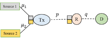
Figure 1: A multi-source relaying status update system in which different status updates arrive at random time slots at Tx which then sends the packets to D via R. For example, in a vehicular setting, sources can be considered as different status information (e.g., speed and location), Tx can be one vehicle’s transmitter called on-board unit [15], R can be another vehicle, and D can be an RSU or a vehicle.

$\bullet$ Wireless Channels: We assume an unreliable channel with transmission success probability $p$ and $q$ for the Tx-R link and R-D link, respectively. Let $\rho[t]$ (resp. $\rho^{\prime}[t]$) be a binary indicator that represents the success of a packet transmission at the Tx-R link (resp. the R-D link) in slot $t$. In specific, if $\rho[t]=1$ (resp. $\rho^{\prime}[t]=1$), the transmitted packet in slot $t$ from Tx (resp. R) is successfully received by R (resp. D); otherwise, $\rho[t]=0$ (resp. $\rho^{\prime}[t]=0$). Thus, $\Pr\{\rho[t]=1\}=p$ and $\Pr\{\rho^{\prime}[t]=1\}=q$. We assume that the perfect feedback (delay-free and error-free) is available at each link.
$\bullet$ Decision Variables: We assume that, in each slot, at most one source can be scheduled per link and the transmissions are over orthogonal channels. Let $\alpha[t]\in\{0,1,2\}$ denote the (transmission) decision of Tx in slot $t$, where $\alpha[t]=i$ means that Tx transmits the packet of source $i$ to R, and $\alpha[t]=0$ means Tx stays idle. Similarly, let $\beta[t]\in\{0,1,2\}$ denote the (transmission) decision of R in slot $t$, where $\beta[t]=i$ means that R forwards the packet of source $i$ to D, and $\beta[t]=0$ means that R stays idle. We assume that there is a centralized controller that decides what Tx and R does during each slot.
$\bullet$ AoI: Let $\theta_{i}[t]$, $\delta_{i}[t]$, and $\Delta_{i}[t]$ be the AoI of source $i$ at Tx, R, and D, in slot $t$, respectively. The evolution of these AoIs are given by

$$\theta_{i}[t+1]=\begin{cases}0,&\text{if}\leavevmode\nobreak\ \leavevmode\nobreak\ \Lambda_{i}[t+1]=1,\\ \theta_{i}[t]+1,&\text{otherwise}\end{cases},$$

$$\delta_{i}[t+1]=\begin{cases}\theta_{i}[t]+1&\text{if}\leavevmode\nobreak\ \leavevmode\nobreak\ \alpha[t]=i,\leavevmode\nobreak\ \rho[t]=1,\\ \delta_{i}[t]+1,&\text{otherwise}\end{cases},$$

$$\Delta_{i}[t+1]=\begin{cases}\delta_{i}[t]+1,&\text{if}\leavevmode\nobreak\ \leavevmode\nobreak\ \beta[t]=i,\leavevmode\nobreak\ \rho^{\prime}[t]=1,\\ \Delta_{i}[t]+1,&\text{otherwise}\end{cases}.$$

II-B Problem Formulation

Let $\mathcal{D}=\{(\alpha[t],\beta[t])\leavevmode\nobreak\ \big{|}\leavevmode\nobreak\ \alpha[t],\beta[t]\in\{0,1,2\}\}$, $t=1,2,3,\dots$, be a sequence of decision variables. We intend to optimize the decision variables in order to minimize the time average sum of AoIs at D, satisfying: i) the transmission capacity constraint per link at every slot and ii) a long-run average resource constraint. Let $\bar{\Delta}(\mathcal{D})$ and $\bar{c}(\mathcal{D})$ denote the long-run expected (time) average sum of AoIs at D and the average number of transmissions in the system, respectively, for given $\mathcal{D}$, which are defined as

$$\begin{array}[]{ll}&\displaystyle\bar{\Delta}(\mathcal{D})\triangleq\limsup_{T\rightarrow\infty}\frac{1}{T}\mathbb{E}\left[\sum_{t=1}^{T}\Delta_{1}[t]+\Delta_{2}[t]\right],\\ &\displaystyle\bar{c}(\mathcal{D})\triangleq\limsup_{T\rightarrow\infty}\frac{1}{T}\mathbb{E}\left[\sum_{t=1}^{T}\mathds{1}_{\{\alpha[t]\neq 0\}}+\mathds{1}_{\{\beta[t]\neq 0\}}\right],\end{array}$$

where $\mathds{1}_{\{\cdot\}}$ is an indicator function which equals to $1$ when the condition in $\{\cdot\}$ holds, and $\mathbb{E}\{\cdot\}$ is the expectation with respect to the system randomness (i.e., channel reliability and packet arrival processes) and the policy. By these definitions, our aim is to solve the following stochastic optimization problem

$$\underset{\mathcal{D}}{\text{minimize}}\leavevmode\nobreak\ \leavevmode\nobreak\ \leavevmode\nobreak\ \leavevmode\nobreak\ \bar{\Delta}(\mathcal{D})$$ (1a)

subject to $$\bar{c}(\mathcal{D})\leq\Gamma_{\max},$$ (1b)

where the real value $\Gamma_{\max}\in(0,2]$ is the maximum allowable average number of transmissions in the system. Constraint (1b) is an average resource constraint that reflects the resource limitation in the normalized form, i.e., normalized to the power usage per each transmission. Thus the constraint can represent a limitation on the total average consumed power.

III CMDP Formulation and Lagrange Relaxation

In this section, we attain to solve main problem (1) by transforming it into a CMDP problem which is then solved by using the Lagrangian relaxation method.

III-A CMDP Formulation

We introduce the CMDP by the following elements:
$\bullet$ State: The state of the CMDP incorporates the knowledge about the AoIs at Tx, R, and D. We define the state in slot $t$ by $\mathbb{s}[t]\triangleq(\theta_{1}[t],x_{1}[t],y_{1}[t],\theta_{2}[t],x_{2}[t],y_{2}[t])$, where $x_{i}[t]\triangleq\delta_{i}[t]-\theta_{i}[t]$ and $y_{i}[t]\triangleq\Delta_{i}[t]-\delta_{i}[t]$ are the relative AoIs at R and D in slot $t$, respectively. Using the relative AoIs simplifies the subsequent analysis and derivations. The intuition is that the amount of the change of the sum AoIs at D from slot $t$ to the next slot $t+1$ is determined by $y_{i}[t]$, which is shown in the following equation

$$\sum_{i}\Delta_{i}[t+1]-\sum_{i}\Delta_{i}[t]=2-\mathds{1}_{\{\beta[t]=i,\rho^{\prime}[t]=1\}}(\underbrace{\Delta_{i}[t]-\delta_{i}[t]}_{y_{i}[t]}).$$

Similarly, the amount of the change of the AoI at R is $x_{i}[t]$. Moreover, we denote the state space by $\mathcal{S}$ which includes all possible states. Note that $\mathcal{S}$ is a countable infinite set due to the AoIs being potentially unbounded.
$\bullet$ Action: We define the action taken in slot $t$ by $\mathbb{a}[t]=(\alpha[t],\beta[t])$, where $\alpha[t],\beta[t]\in\{0,1,2\}$. Actions are determined by a policy, denoted by $\pi$, which is a rule that generates these actions by observing the current state (i.e., Markovian policies), i.e., a policy is a mapping from states to actions, potentially with a probability distribution. Moreover, let $\mathcal{A}$ denote the action space.
$\bullet$ Cost Functions: The (immediate) cost functions include: 1) the AoI cost, and 2) the transmission cost. The AoI cost of each slot $t$ is the sum AoIs at D given by $C(\mathbb{s}[t])=\sum_{i}\theta_{i}[t]+x_{i}[t]+y_{i}[t].$ The transmission cost of slot $t$, for action $\mathbb{a}[t]$ is defined by $D(\mathbb{a}[t])=\mathds{1}_{\{\alpha[t]\neq 0\}}+\mathds{1}_{\{\beta[t]\neq 0\}}.$
$\bullet$ State Transition Probabilities: For any two states $\mathbb{s},\mathbb{s}^{\prime}\in\mathcal{S}$, $\mathcal{P}_{\mathbb{s}\mathbb{s}^{\prime}}(\mathbb{a})$ is the state transition probability that gives the probability of moving to state $\mathbb{s}^{\prime}$ (next state) from state $\mathbb{s}$ (current state) under taking an action $\mathbb{a}=(\alpha,\beta)$. Mathematically, $\mathcal{P}_{\mathbb{s}\mathbb{s}^{\prime}}(\mathbb{a})$ is given as $\mathcal{P}_{\mathbb{s}\mathbb{s}^{\prime}}(\mathbb{a})=\prod_{i}\Pr\{\mathbb{s}_{i}^{\prime}|\mathbb{s}_{i},\mathbb{a}\}$, where $\mathbb{s}^{\prime}_{i}=(\theta^{\prime}_{i},x^{\prime}_{i},y^{\prime}_{i}),\leavevmode\nobreak\ \mathbb{s}_{i}=(\theta_{i},x_{i},y_{i})$ are state vectors associated to source $i$, and $\Pr\{\mathbb{s}_{i}^{\prime}|\mathbb{s}_{i},\mathbb{a}\}$ is given by (2) shown on the top of next page. Note that $\mathbb{s}$ is arranged as $\mathbb{s}=(\mathbb{s}_{1},\mathbb{s}_{2})$.

$$\small\Pr\{\mathbb{s}_{i}^{\prime}|\mathbb{s}_{i}=(\theta_{i},x_{i},y_{i}),\mathbb{a}=(\alpha,\beta)\}=\begin{cases}\mu_{i}pq,&\alpha=i,\beta=i;\leavevmode\nobreak\ \theta^{\prime}_{i}=0,\leavevmode\nobreak\ x^{\prime}_{i}=\theta_{i}+1,\leavevmode\nobreak\ y^{\prime}_{i}=x_{i},\\ \mu_{i}(1-p)q,&\alpha=i,\beta=i;\leavevmode\nobreak\ \theta^{\prime}_{i}=0,\leavevmode\nobreak\ x^{\prime}_{i}=x_{i}+\theta_{i}+1,\leavevmode\nobreak\ y^{\prime}_{i}=0,\\ \mu_{i}p(1-q),&\alpha=i,\beta=i;\leavevmode\nobreak\ \theta^{\prime}_{i}=0,\leavevmode\nobreak\ x^{\prime}_{i}=\theta_{i}+1,\leavevmode\nobreak\ y^{\prime}_{i}=y_{i}+x_{i},\\ \mu_{i}(1-p)(1-q),&\alpha=i,\beta=i;\leavevmode\nobreak\ \theta^{\prime}_{i}=0,\leavevmode\nobreak\ x^{\prime}_{i}=x_{i}+\theta_{i}+1,\leavevmode\nobreak\ y^{\prime}_{i}=y_{i},\\ (1-\mu_{i})pq,&\alpha=i,\beta=i;\leavevmode\nobreak\ \theta^{\prime}_{i}=\theta_{i}+1,\leavevmode\nobreak\ x^{\prime}_{i}=0,\leavevmode\nobreak\ y^{\prime}_{i}=x_{i},\\ (1-\mu_{i})(1-p)q,&\alpha=i,\beta=i;\leavevmode\nobreak\ \theta^{\prime}_{i}=\theta_{i}+1,\leavevmode\nobreak\ x^{\prime}_{i}=x_{i},\leavevmode\nobreak\ y^{\prime}_{i}=0,\\ (1-\mu_{i})p(1-q),&\alpha=i,\beta=i;\leavevmode\nobreak\ \theta^{\prime}_{i}=\theta_{i}+1,\leavevmode\nobreak\ x^{\prime}_{i}=0,\leavevmode\nobreak\ y^{\prime}_{i}=y_{i}+x_{i},\\ {(1-p)(1-q)(1-\mu_{i})},&\alpha=i,\beta=i;\leavevmode\nobreak\ \theta^{\prime}_{i}=\theta_{i}+1,\leavevmode\nobreak\ x^{\prime}_{i}=x_{i},\leavevmode\nobreak\ y^{\prime}_{i}=y_{i},\\ \mu_{i}p,&\alpha=i,\beta\neq i;\leavevmode\nobreak\ \theta^{\prime}_{i}=0,\leavevmode\nobreak\ x^{\prime}_{i}=\theta_{i}+1,\leavevmode\nobreak\ y^{\prime}_{i}=y_{i}+x_{i},\\ \mu_{i}(1-p),&\alpha=i,\beta\neq i;\leavevmode\nobreak\ \theta^{\prime}_{i}=0,\leavevmode\nobreak\ x^{\prime}_{i}=x_{i}+\theta_{i}+1,\leavevmode\nobreak\ y^{\prime}_{i}=y_{i},\\ (1-\mu_{i})p,&\alpha=i,\beta\neq i;\leavevmode\nobreak\ \theta^{\prime}_{i}=\theta_{i}+1,\leavevmode\nobreak\ x^{\prime}_{i}=0,\leavevmode\nobreak\ y^{\prime}_{i}=y_{i}+x_{i},\\ (1-\mu_{i})(1-p),&\alpha=i,\beta\neq i;\leavevmode\nobreak\ \theta^{\prime}_{i}=\theta_{i}+1,\leavevmode\nobreak\ x^{\prime}_{i}=x_{i},\leavevmode\nobreak\ y^{\prime}_{i}=y_{i},\\ \mu_{i}q,&\alpha\neq i,\beta=i;\leavevmode\nobreak\ \theta^{\prime}_{i}=0,\leavevmode\nobreak\ x^{\prime}_{i}=x_{i}+\theta_{i}+1,\leavevmode\nobreak\ y^{\prime}_{i}=0,\\ \mu_{i}(1-q),&\alpha\neq i,\beta=i;\leavevmode\nobreak\ \theta^{\prime}_{i}=0,\leavevmode\nobreak\ x^{\prime}_{i}=x_{i}+\theta_{i}+1,\leavevmode\nobreak\ y^{\prime}_{i}=y_{i},\\ (1-\mu_{i})q,&\alpha\neq i,\beta=i;\leavevmode\nobreak\ \theta^{\prime}_{i}=\theta_{i}+1,\leavevmode\nobreak\ x^{\prime}_{i}=x_{i},\leavevmode\nobreak\ y^{\prime}_{i}=0,\\ (1-\mu_{i})(1-q),&\alpha\neq i,\beta=i;\leavevmode\nobreak\ \theta^{\prime}_{i}=\theta_{i}+1,\leavevmode\nobreak\ x^{\prime}_{i}=x_{i},\leavevmode\nobreak\ y^{\prime}_{i}=y_{i},\\ \mu_{i},&\alpha\neq i,\beta\neq i;\leavevmode\nobreak\ \theta^{\prime}_{i}=0,\leavevmode\nobreak\ x^{\prime}_{i}=x_{i}+\theta_{i}+1,\leavevmode\nobreak\ y^{\prime}_{i}=y_{i},\\ 1-\mu_{i},&\alpha\neq i,\beta\neq i;\leavevmode\nobreak\ \theta^{\prime}_{i}=\theta_{i}+1,\leavevmode\nobreak\ x^{\prime}_{i}=x_{i},\leavevmode\nobreak\ y^{\prime}_{i}=y_{i},\\ 0&\text{otherwise},\end{cases}$$ (2)

 

By these definitions, the objective of CMDP, denoted by $J(\pi;\mathbb{s}[0])$, which is the expected average sum AoIs at D, is given by

$$J(\pi;\mathbb{s}[0])=\limsup_{T\rightarrow\infty}\frac{1}{T}\mathbb{E}\left[\sum_{t=1}^{T}C(\mathbb{s}[t])\leavevmode\nobreak\ \big{|}\leavevmode\nobreak\ \mathbb{s}[0]\right],$$

where $\mathbb{s}[0]$ is the initial state. Similarly, the constraint function of CMDP, denoted by $\bar{D}(\pi;\mathbb{s}[0])$, which is the expected average transmission cost in the system, is given by

$$\bar{D}(\pi;\mathbb{s}[0])=\limsup_{T\rightarrow\infty}\frac{1}{T}\mathbb{E}\left[\sum_{t=1}^{T}{D(\mathbb{a}[t])}{}\leavevmode\nobreak\ \big{|}\leavevmode\nobreak\ \mathbb{s}[0]\right].$$

Now, problem (1) is transformed into the following CMDP problem

$$\underset{\pi}{\text{minimize}}\leavevmode\nobreak\ \leavevmode\nobreak\ \leavevmode\nobreak\ \leavevmode\nobreak\ J(\pi;\mathbb{s}[0])$$ (3a)

subject to $$\bar{D}(\pi;\mathbb{s}[0])\leq\Gamma_{\max}.$$ (3b)

The optimal value of problem (3) for a given $\mathbb{s}[0]$ is denoted by $J^{*}(\mathbb{s}[0])$.

III-B Lagrange Relaxation Method

We transform problem (3) into an unconstrained average cost MDP (or simply MDP) leveraging the Lagrangian relaxation method. By this method, for a given Lagrange multiplier ${\lambda}\geq 0$, the Lagrangian, acting as the objective function for the MDP problem, is given by $\mathcal{L}(\pi,{{\lambda}};\mathbb{s}[0])\triangleq\limsup_{T\rightarrow\infty}\frac{1}{T}\left(\mathbb{E}\left[\sum_{t=1}^{T}C(\mathbb{s}[t])+\lambda D(\mathbb{a}[t])\leavevmode\nobreak\ |\leavevmode\nobreak\ \mathbb{s}[0]\right]\right)$. Note that the term $-\lambda\Gamma_{\max}$ is omitted from the Lagrangian because of being constant with respect to the policy for a given $\lambda$. An optimal policy of the MDP, for fixed $\lambda$, denoted by $\pi^{*}_{\lambda}$ and called MDP-optimal policy, is a solution of the following MDP problem:

$$\underset{\pi_{\lambda}}{\text{minimize}}\leavevmode\nobreak\ \leavevmode\nobreak\ \leavevmode\nobreak\ \mathcal{L}(\pi_{\lambda},{{\lambda}};\mathbb{s}[0]).$$ (4)

By checking the growth condition [17, Eq. 11.20], the optimal value of the CMDP problem (3), $J^{*}(\mathbb{s}[0])$, and the optimal value of the MDP problem (4), denoted by $\mathcal{L}^{*}({{\lambda}};\mathbb{s}[0])$, ensures the following:

$$J^{*}(\mathbb{s}[0])=\sup_{\lambda\geq 0}\leavevmode\nobreak\ \mathcal{L}^{*}({{\lambda};\mathbb{s}[0]})-\lambda\Gamma_{\max}.$$ (5)

Therefore, the solution of the CMDP problem (3) can be found by an algorithm that iteratively executes the following two steps: 1) find an optimal policy of the MDP problem (4) with fixed $\lambda$, i.e., $\pi_{\lambda}^{*}$, and 2) update $\lambda$ to a direction that aims to obtain $J^{*}(\mathbb{s}[0])$ according to (5).
In the next section, we focus to find an MDP-optimal policy $\pi^{*}_{\lambda}$ and estimating the optimal Lagrange multiplier.

IV Optimal Policy of the CMDP Problem

In the following, we focus on obtaining an MDP-optimal policy and estimating the optimal Lagrange multiplier, respectively, in Sec. IV-A and Sec. IV-B.

IV-A Optimal Policy of the MDP Problem

We elaborate on the structure of MDP-optimal policy for the case with error-free links by the following theorem.

Theorem 1.

For given $\lambda$ and error-free links, any MDP-optimal policy of problem (4) has a switching-type structure for $\beta$ with respect to $\mathbb{y}=(y_{1},y_{2})$.

Proof.

The proof will be provided in the extended version. ∎

Value iteration is a classical method to handle MDP problems, but cannot be applied for the infinite state spaces. To circumvent this problem, we use the state truncation method and approximation analysis [17, Ch. 16],[18].

IV-A1 State Truncation and Approximated MDP

We truncate $\mathcal{S}$ into a finite state space $\mathcal{S}^{(N)}$ which is parameterized by an integer $N$. To this end, whenever the AoIs exceed $N$, we set their values to $N$. The corresponding MDP is called the truncated or approximated MDP. The state transition probabilities of the truncated MDP, $\mathcal{P}_{\mathbb{s}\mathbb{s}^{\prime}}^{(N)}(\mathbb{a})$, are obtained by Eq. (2) under the following changes. In all equations of Eq. (2), we replace $\theta_{i}+1,\leavevmode\nobreak\ x_{i},$ and $y_{i}$, respectively, by $\theta_{i}+1\rightarrow\big{[}\theta_{i}+1\big{]}_{N}^{+}$, $x_{i}\rightarrow\big{[}x_{i}+\theta_{i}+1\big{]}_{N}^{+}-\big{[}\theta_{i}+1\big{]}_{N}^{+}$ and $y_{i}\rightarrow\big{[}y_{i}+x_{i}+\theta_{i}+1\big{]}_{N}^{+}-\big{[}x_{i}+\theta_{i}+1\big{]}_{N}^{+}$, where $\big{[}z\big{]}_{N}^{+}$ equals to $z$ if $z\leq N$; otherwise, it equals to $N$. In general, there is no guarantee that the truncated MDP converges to the original one [18, p. 276]. By [16, Theorem 9], for large enough $N$, the truncated MDP convergences to the original MDP.

IV-A2 Finding Optimal Policy of the Truncated MDP

Now, the Relative Value Iteration (RVI) algorithm can be exploited to solve the truncated MDP for a given $\lambda$ and parameter $N$. In specific, RVI is an iterative algorithm with the following value iteration equation with iteration index $n$:

$$V_{n+1}^{(N)}(\mathbb{s})=\min_{\mathbb{a}}\left\{L(\mathbb{s},\mathbb{a};\lambda)+\mathbb{E}[h_{n}^{(N)}(\mathbb{s}^{\prime})]\right\},$$

where $L(\mathbb{s},\mathbb{a};\lambda)=C(\mathbb{s})+\lambda D(\mathbb{a})$ and $h_{n}^{(N)}(\mathbb{s}^{\prime})\triangleq V_{n}^{(N)}(\mathbb{s}^{\prime})-V_{n}^{(N)}(\mathbf{s}_{\mathrm{ref}})$ is the relative value function, $\mathbf{s}_{\mathrm{ref}}$ is a reference state, and $V_{0}^{(N)}(\mathbf{s}_{\mathrm{ref}})=0$. Moreover, $\mathbb{E}[h_{n}^{(N)}(\mathbb{s}^{\prime})]=\underset{\mathbb{s}^{\prime}\in\mathcal{S}^{(N)}}{\sum}\mathcal{P}^{(N)}_{\mathbb{s}\mathbb{s}^{\prime}}(\mathbb{a})h_{n}^{(N)}(\mathbb{s}^{\prime})$. The details of RVI are provided in Alg. 1 (see Steps 3-11), where $\varepsilon$ is a RVI termination criterion.
For a given $N$ and $\lambda$, the RVI algorithm give an optimal policy for the truncated MDP after a finite number of iterations. This is because the truncated state MDP is unichain and by [19, Theorem 8.6.6] the optimality of RVI is guaranteed.

IV-B Estimating Optimal Lagrange Multiplier

By [20, Lemma 3.4], for $\lambda>0$, $J(\pi^{*}_{\lambda})$ and $\mathcal{L}(\pi_{\lambda}^{*};\lambda)$ ($\mathbb{s}[0]$ is omitted) are increasing in $\lambda$ and $\bar{D}(\pi^{*}_{\lambda})$ is decreasing in $\lambda$. Therefore, the optimal Lagrange multiplier $\lambda^{*}$ is given by

$$\lambda^{*}=\inf\{\lambda>0:\bar{D}(\pi^{*}_{\lambda})\leq\Gamma_{\max}\}.$$ (6)

As a result, if we find $\pi^{*}_{\lambda^{*}}$ such that $\bar{D}(\pi^{*}_{\lambda^{*}})=\Gamma_{\max}$, then $\pi^{*}_{\lambda^{*}}$ is an optimal policy for the CMDP problem (3). Exploiting the monotonicity of $\bar{D}(\pi^{*}_{\lambda})$ with respect to $\lambda$, we adopt the bisection search [21, 22] to find $\lambda^{*}$. Details are stated in Alg. 1, where we initialize $\lambda^{-}=0$ and $\lambda^{+}$ as a large positive real number, and $\zeta$ is a sufficiently small positive real number for the bisection termination criterion.
Importantly, there is no guarantee (roughly, no possibility), even for any arbitrarily small $\zeta$, that $\pi^{*}_{\lambda_{\mathrm{bis}}}$ obtained by Alg. 1 would ensure that $\bar{D}(\pi^{*}_{\lambda_{\mathrm{bis}}})=\Gamma_{\max}$. This is, $\pi^{*}_{\lambda_{\mathrm{bis}}}$ (resp. $J(\pi^{*}_{\lambda_{\mathrm{bis}}})$) is not necessarily an optimal policy (resp. the optimal value) for the CMDP problem (3). Following [23], by exploiting a mixing policy which is mixture of $\pi^{*}_{\lambda^{-}}$ (infeasible policy) and $\pi^{*}_{\lambda^{+}}$ (feasible policy) with mixing factor $\eta$, the value of CMDP problem (3), $J_{\mathrm{mix}}$, is given by

$$J_{\mathrm{mix}}=\eta J(\pi^{*}_{\lambda^{+}})+(1-\eta)J(\pi^{*}_{\lambda^{-}}),$$ (7)

where

$$\eta=\frac{\Gamma_{\max}-\bar{D}(\pi^{*}_{\lambda^{-}})}{\bar{D}(\pi^{*}_{\lambda^{+}})-\bar{D}(\pi^{*}_{\lambda^{-}})}.$$ (8)

We remark that although $J_{\mathrm{mix}}$ is less than $J(\pi^{*}_{\lambda^{+}})$, there is no guarantee that $J_{\mathrm{mix}}$ is the optimal value of the CMDP problem (3). This is because there are no guarantees that $\pi^{*}_{\lambda^{-}}$ and $\pi^{*}_{\lambda^{+}}$ are converged policies, i.e., as $\lambda^{-}$ increases to $\lambda^{*}$, the corresponding $\pi^{*}_{\lambda^{-}}$ does not change (similarly for $\lambda^{+}$ as it decreases to $\lambda^{*}$) [24, 20]. However, $J_{\mathrm{mix}}$ serves as a benchmark to evaluate the performance of any policy such as $\pi^{*}_{\lambda^{+}}$.
Finally, we note that the mixing policy is not stationary and ergodic. Accordingly, one can select $\pi^{*}_{\lambda^{+}}$ as a feasible solution for the CMDP problem (3) which is a stationary deterministic policy and is more desirable in practice. As explained before, policy $\pi^{*}_{\lambda^{+}}$ is not guaranteed to be an optimal policy for the CMDP problem (3), while it gives acceptable performance for small enough $\zeta$, as shown in the numerical analysis.

Input: $N,\leavevmode\nobreak\ \zeta,\leavevmode\nobreak\ \varepsilon,\leavevmode\nobreak\ \lambda^{+},\leavevmode\nobreak\ \lambda^{-},\leavevmode\nobreak\ \Gamma_{\max},\leavevmode\nobreak\ \mu_{1},\leavevmode\nobreak\ \mu_{2},\leavevmode\nobreak\ p,\leavevmode\nobreak\ q$

1 while  $|\lambda^{+}-\lambda^{-}|\geq\zeta$ do

2      

3      $\lambda_{\mathrm{bis}}=\frac{\lambda^{+}+\lambda^{-}}{2}$;

4      For all $\mathbb{s}\in\mathcal{S}^{(N)},\leavevmode\nobreak\ \text{set}\leavevmode\nobreak\ V^{(N)}(\mathbb{s})=0,\leavevmode\nobreak\ h^{(N)}(\mathbb{s})=0,\leavevmode\nobreak\ h^{(N)}_{\mathrm{old}}(\mathbb{s})=1$;

5      

6      while $\max_{\mathbb{s}\in\mathcal{S}^{(N)}}|h^{(N)}(\mathbb{s})-h^{(N)}_{\mathrm{old}}(\mathbb{s})|>\varepsilon$ do

7            

8            foreach $\mathbb{s}\in\mathcal{S}^{(N)}$ do

9                  

10                  $\mathbb{a}^{*}\leftarrow\underset{\mathbb{a}}{\arg\min}\leavevmode\nobreak\ \leavevmode\nobreak\ L(\mathbb{s},\mathbb{a};\lambda_{\mathrm{bis}})+\mathbb{E}\{h^{(N)}(\mathbb{s}^{\prime}\}$;

11                  

12                  $V^{(N)}(\mathbb{s})\leftarrow L(\mathbb{s},\mathbb{a}^{*};\lambda_{\mathrm{bis}})+\mathbb{E}\{h^{(N)}(\mathbb{s}^{\prime})\}$;

13                  

14                  $h^{(N)}_{\mathrm{tmp}}(\mathbb{s})\leftarrow V^{(N)}(\mathbb{s})-V^{(N)}(\mathbf{s}_{\mathrm{ref}})$;

15                  

16             end foreach

17            $h^{(N)}_{\text{old}}(\mathbb{s})\leftarrow h^{(N)}(\mathbb{s})$, $h^{(N)}(\mathbb{s})\leftarrow h^{(N)}_{\mathrm{tmp}}(\mathbb{s})$;

18            

19       end while

20      

21      Compute $\bar{D}(\pi^{*}_{\lambda_{\mathrm{bis}}})$;

22      

23      if $\bar{D}(\pi^{*}_{\lambda_{\mathrm{bis}}})\geq\Gamma_{\max}$ then

24            

25            $\lambda^{-}\leftarrow\lambda_{\mathrm{bis}}$;

26            

27      else

28             $\lambda^{+}\leftarrow\lambda_{\mathrm{bis}}$;

29            

30       end if

31      

32 end while

33Compute $\pi^{*}_{\lambda^{+}}$ and $\pi^{*}_{\lambda^{-}}$;

34

35Compute $\bar{D}(\pi^{*}_{\lambda^{+}})$ and $\bar{D}(\pi^{*}_{\lambda^{-}})$, and then $\eta^{*}$ by (8);

36

37Compute $J(\pi^{*}_{\lambda^{+}})$ and $J(\pi^{*}_{\lambda^{-}})$;

38

39Compute $J_{\mathrm{mix}}=\eta J(\pi^{*}_{\lambda^{+}})+(1-\eta)J(\pi^{*}_{\lambda^{-}})$;

40

Output: $\pi^{*}_{\lambda^{+}},\leavevmode\nobreak\ J_{\mathrm{mix}}$

41

Algorithm 1 Policy design for the CMDP problem (3) via RVI and bisection search

V Numerical Results

In this section, we numerically evaluate the AoI performance of the proposed algorithm (Alg. 1) and the structure of an optimal policy. The system parameters including the values of the arrival rates, $\mu=(\mu_{1},\mu_{2})$, the reliabilities of the links in the system, $p$ and $q$, and the allowable average number of transmissions, $\Gamma_{\max}$, are stated in the label or legend of each figure. For Alg. 1, we set $N=7$, $\zeta=0.01$, and $\varepsilon=0.001$.
Fig. 2 shows an example of the structure of the policy for the decision at R, $\beta$, with respect to the relative AoIs at D, $y_{i}$, for state $\mathbb{s}=(1,2,0,1,y_{1},y_{2})$. This figure verifies Theorem 1, and unveils that R schedules the available packet of the source with a higher relative AoI at D.

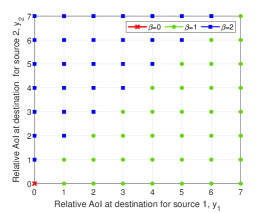
Figure 2: An illustration of the switching-type structure for state $\mathbb{s}=(1,2,0,1,y_{1},y_{2})$ with respect to $\beta$, for $p=0.8,\leavevmode\nobreak\ q=0.7,\leavevmode\nobreak\ \Gamma_{\max}=1.6$, and $\mu=(0.6,0.9)$.

Fig. 3 exemplifies the structure of the policy for the decision at Tx, $\alpha$, with respect to the relative AoIs at R, $x_{i}$, for state ${\mathbb{s}=(1,1,x_{1},x_{2},4,4)}$. Having $\alpha=0$ at ($x_{1}=0$, $x_{2}=1$) implies that transmission does not occur at every state due to the resource budget. We can conclude from this figure that for fixed $y_{1}$ and $y_{2}$, Tx will give a higher priority to schedule the source that has a lower status update rate. This is because the waiting time at D for receiving new updates from that source becomes large as a consequence of infrequent packet arrivals, which becomes a bottleneck in reducing the AoI.

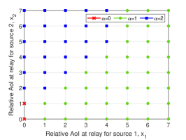
Figure 3: An illustration of the switching-type structure for state $\mathbb{s}=(1,1,x_{1},x_{2},4,4)$ with respect to $\alpha$, for $p=0.8,\leavevmode\nobreak\ q=0.7,$ and $\Gamma_{\max}=1.6,\leavevmode\nobreak\ \mu=(0.6,0.9)$.

Fig. 4 depicts the average sum AoI at D (sum AAoI) with respect to the allowable average number of transmissions in the system (resource budget), $\Gamma_{\max}$, for different arrival rates and reliability of the links, obtained by averaging over 100,000 time slots. In this figure, “Mix.” refers to $J_{\mathrm{mix}}$ obtained by (7), and “Deter.” stands for $J(\pi^{*}_{\lambda^{+}})$. For benchmarking, we consider a “Lower bound” scheme where we eliminate the average resource constraint by setting $\Gamma_{\max}=2$ and realize the generate-at-will model by setting the arrival rates as ${\mu_{1}=\mu_{2}=1}$. With these setting, our system becomes equivalent to the one studied in [6], and we use the greedy-based optimal policy derived in [6]. As another benchmark, we design a “Greedy” policy, where the transmission is allowed in slot $t$ when $\bar{D}_{t}\leq\Gamma_{\max}$, where $\bar{D}_{t}$ denotes the average number of transmissions until $t$, and the decision criteria are the relative AoI at R for $\alpha$ and the relative AoI at D for $\beta$.
First, Fig. 4 shows that the deterministic policy, $\pi^{*}_{\lambda^{+}}$, achieves a near-optimal performance. Fig. 4 illustrates that the sum AAoI dramatically increases when the resource budget $\Gamma_{\max}$ is decreased, and the sum AAoI values become large when channel reliabilities are reduced. Moreover, Fig. 4 exhibit that the sum AAoI converges to the lower bound when the arrival rates of updates are high and the resource budget is large. For that case, we infer that an optimal policy has a greedy behavior where the maximum of the relative AoIs at R is the greedy criterion for the decision of Tx, and the maximum of the relative AoIs at D is a greedy criterion for the decision of R. We observe that the optimality gap for the Greedy policy is large when the resource budget is small. This clearly emphasizes that it is pivotal to take into account resource limitations in age-optimal policy design. Namely, it may be possible to find some algorithms that minimize the sum AAoI, but they are not necessarily resource-efficient ones.

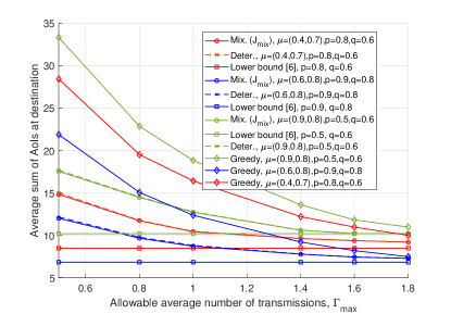
Figure 4: Average sum AoIs at D versus $\Gamma_{\max}$, for different arrival rates $\mu=(\mu_{1},\mu_{2})$, and reliability of channels, $p$ and $q$.

VI Conclusion

We studied the sum AAoI minimization scheduling problem in a multi-source relaying system with stochastic arrivals and unreliable communication channels, under per-slot transmission capacity constraints per link and a long-run average resource constraint. To this end, we formulated a stochastic optimization problem and recast it as a CMDP problem. We analyzed the structure of an optimal policy and proposed an algorithm that obtains a stationary deterministic near-optimal policy which is easy to implement. According to the simulation results, our proposed algorithm significantly reduces the sum AAoI compared with the non-trivial greedy-based benchmark algorithm. We concluded that when the average resource budget is large and the arrival rates of status updates are high, an optimal policy has a greedy behavior.

VII Acknowledgments

This research has been financially supported by the Infotech Oulu, the Academy of Finland (grant 323698), and Academy of Finland 6Genesis Flagship (grant 318927). The work of M. Leinonen has also been financially supported in part by the Academy of Finland (grant 319485).

References

• [1] M. A. Abd-Elmagid, N. Pappas, and H. S. Dhillon, “On the role of age of information in the internet of things,” IEEE Commun. Mag, vol. 57, no. 12, pp. 72–77, Dec. 2019.
• [2] E. Altman, R. El-Azouzi, D. S. Menasche, and Y. Xu, “Forever young: Aging control for smartphones in hybrid networks,” CoRR, Sep. 2010.
• [3] S. Kaul, R. Yates, and M. Gruteser, “Real-time status: How often should one update?,” in Proc. IEEE Int. Conf. on Computer Commun., pp. 2731–2735, Orlando, FL, USA, Mar. 2012.
• [4] M. Moltafet, M. Leinonen, and M. Codreanu, “On the age of information in multi-source queueing models,” IEEE Trans. Commun., vol. 68, no. 8, pp. 5003–5017, Aug. 2020.
• [5] M. Costa, M. Codreanu, and A. Ephremides, “On the age of information in status update systems with packet management,” IEEE Trans. Inf. Theory, vol. 62, no. 4, pp. 1897–1910, Apr. 2016.
• [6] J. Song, D. Gunduz, and W. Choi, “Optimal scheduling policy for minimizing age of information with a relay,” arXiv, preprint arXiv:2009.02716., Sep. 2020.
• [7] M. Hatami, M. Leinonen, and M. Codreanu, “AoI minimization in status update control with energy harvesting sensors,” arXiv preprint arXiv:2009.04224, Sep. 2020.
• [8] Y. Gu, Q. Wang, H. Chen, Y. Li, and B. Vucetic, “Optimizing information freshness in two-hop status update systems under a resource constraint,” IEEE J. Sel. Areas Commun., vol. 39, no. 5, pp. 1380–1392, May, 2021.
• [9] M. Moltafet, M. Leinonen, M. Codreanu, and N. Pappas, “Power minimization for age of information constrained dynamic control in wireless sensor networks,” arXiv preprint arXiv:2007.05364, Jul. 2020.
• [10] M. Moradian and A. Dadlani, “Age of information in scheduled wireless relay networks,” in Proc. IEEE Wireless Commun. and Netw. Conf. (WCNC), pp. 1–6, Seoul, Korea (South), Mar. 2020.
• [11] B. Li, H. Chen, N. Pappas, and Y. Li, “Optimizing information freshness in two-way relay networks,” in Proc. IEEE/CIC Int. Conf. on Commun. in China (ICCC), pp. 893–898, Chongqing, China, Aug. 2020.
• [12] A. M. Bedewy, Y. Sun, and N. B. Shroff, “Age-optimal information updates in multihop networks,” in Proc. IEEE Int. Symp. Inform. Theory, pp. 576–580, Aachen, Germany, Jun. 2017.
• [13] A. Arafa and S. Ulukus, “Timely updates in energy harvesting two-hop networks: Offline and online policies,” IEEE Trans. Wireless Commun., vol. 18, no. 8, pp. 4017–4030, Aug. 2019.
• [14] B. Li, Q. Wang, H. Chen, Y. Zhou, and Y. Li, “Optimizing information freshness for cooperative IoT systems with stochastic arrivals,” IEEE Internet Things J, Early Access, 2021.
• [15] Z. Su, Y. Hui, T. H. Luan, Q. Liu, and R. Xing, The Next Generation Vehicular Networks, Modeling, Algorithm and Applications. Springer, 2020.
• [16] Y. P. Hsu, E. Modiano, and L. Duan, “Scheduling algorithms for minimizing age of information in wireless broadcast networks with random arrivals,” IEEE Trans. Mobile Comput., vol. 19, no. 12, pp. 2903–2915, Dec. 2020.
• [17] E. Altman, Constrained Markov Decision Processes. volume 7. CRC Press, 1999.
• [18] L. I. Sennott, Stochastic Dynamic Programming and the Control of Queueing Systems. volume 504. John Wiley & Sons, 2009.
• [19] M. L. Puterman, Markov Decision Processes: Discrete Stochastic Dynamic Programming. The MIT Press, 1994.
• [20] L. I. Sennott, “Constrained average cost Markov decision chains,” Probab. Eng. Inf. Sci., vol. 7, no. 1, pp. 69–83, Jan. 1993.
• [21] H. Huang, D. Qiao, and M. C. Gursoy, “Age-energy tradeoff in fading channels with packet-based transmissions,” in Proc. IEEE Int. Conf. on Computer Commun., pp. 323–328, Toronto, ON, Canada, Jul., 2020.
• [22] A. Maatouk, M. Assaad, and A. Ephremides, “The age of incorrect information: an enabler of semantics-empowered communication,” arXiv preprint arXiv:2012.13214, Dec. 2020.
• [23] D.-J. Ma, M. Makowski, and A. Shwartz, “Estimation and optimal control for constrained Markov chains,” In Proceedings of the 25th IEEE Conf. on Decision and Control., pp. 994-999, 1987.
• [24] K. Beutler, F.J. Ross, “Optimal policies for controlled Markov chains with a constraint,” Mathematical Methods of Operations Research, vol. 112, pp. 236-252., 1985.