Bayesian inference of polymerase dynamics over the exclusion process.

Abstract

Transcription is a complex phenomenon that permits the conversion of genetic information into phenotype by means of an enzyme called RNA polymerase, which erratically moves along and scans the DNA template. We perform Bayesian inference over a paradigmatic mechanistic model of non-equilibrium statistical physics, i.e., the asymmetric exclusion processes in the hydrodynamic limit, assuming a Gaussian process prior for the polymerase progression rate as a latent variable. Our framework allows us to infer the speed of polymerases during transcription given their spatial distribution, whilst avoiding the explicit inversion of the system’s dynamics. The results, which show processing rates strongly varying with genomic position and minor role of traffic-like congestion, may have strong implications for the understanding of gene expression.

I Introduction

DNA is a long polymeric molecule that encodes information as a sequence of nucleotides (Nts). Turning this information into a phenotype is a complex phenomenon hinged upon transcription, the molecular process in which particular segments of DNA (i.e., the genes) are scanned and their information is copied into mRNA by the enzyme RNA polymerase II (PolII). The transcription itself consists of several steps which can be differentially regulated to alter the timing and the output of the mRNA production Munsky2012 ; Rajala2010 .

The transcription can also be seen as a non-equilibrium process, where the PolIIs are being transported as particles on a one dimensional lattice, the lattice being the DNA template which the PolIIs bind to. We can further consider this process having left and right boundaries, representing the transcription start site (TSS) and the transcription end site (TES), respectively (Fig. 1 A). Within the gene body, the PolIIs erratically travel along the template and their abrupt slowing down in certain genomic regions is known as pausing dynamics Jonkers2015 ; Mayer2017 . While the pausing is an essential part of the transcriptional machinery and contributes to the regulation of genes’ expression levels, a comprehensive quantitative understanding of its dynamics is still missing Adelman2012 ; Liu2015 .

We present a modelling framework to help understand gene regulation and quantitatively study the pausing dynamics given real-world data. In literature, a number of different mechanistic models have been introduced to elucidate transcription, starting from the simple telegraph model peccoud1995markovian to more complicated multi-state models that account for many interactions Tripathi2008 ; Dobrzynski2009 ; Cao2020 ; Szavits-Nossan2022 , with each model reflecting determinate aspects of the whole biological system complexity. Here we are primarily interested in the pausing and employ a generalisation of a paradigmatic model of particle transport, the asymmetric simple exclusion process (ASEP, MacDonald1968 ; MacDonald69 ; Spitzer1970 ) in the hydrodynamic limit Benassi1987 . The ASEP is a class of models of particles on a one-dimensional lattice, whose behaviour is chiefly determined by the rates at which the particles hop on the lattice. More specifically we require the rate profile function, which we refer to as $\tilde{p}$, to be spatially varying yet smooth as in reference Stinchcombe2011 ; Lakatos2006 , see also Harris2004 , thus making it possible to model this function by a Gaussian process (GP) Rasmussen2006 . Noticing the analogy between the PolII transport in the gene body and the particle hopping in the exclusion process, learning $\tilde{p}$ allows the study of the pausing dynamics in a gene. Importantly, we provide an inferential scheme to learn this rate function by Bayesian inference given real molecular biology data, assuming a prior on the profile function induced by a GP prior on a latent variable. In other words, integrating the dynamics defined by the rate $\tilde{p}$ generates transient time-course density profiles; we estimating $\tilde{p}$ given observed density profiles without explicitly inverting the system’s dynamics. Other models of PolII dynamics also leverage GPs for inference from biological data, with GPs representing transcriptional activity over time WaMaina2014 ; Honkela2015 . In contrast, the GP here describes a function of genomic position, with its minima corresponding to pausing regions. Due to its generality, our framework can be deployed to estimate the rate profiles of any one-dimensional transport problem.

The manuscript is organised as follows. Section II.1 describes the biology of pausing and the next-generation sequencing (NGS) data types which are available to study it. Section II.2 and II.3, respectively, discuss the asymmetric simple exclusion process as a mathematical model for transcription with pausing and a Bayesian inferential framework for model fitting. We present the results in section III and conclude with a discussion in section IV.

II Model definition

II.1 Biological processes and data

RNA polymerases have a central role in the biology of transcription. We distinguish different classes of RNA polymerases, each having different structure and control mechanism. Bacteria and Archaea only have one RNA polymerase type. Eukaryotes have multiple types, of which RNA polymerase II (PolII) is known to catalyse synthesis of protein-encoding RNA (messenger RNA or mRNA). In this paper we describe mRNA transcription by PolII, but the inferential framework we present is general and can be extended to other transport phenomena. PolII binds to DNA upstream the TSS, initiates the mRNA synthesis, and then traverses the DNA downstream (elongation) until it pauses at a certain gene location, ready to respond to a developmental or environmental signal that instructs to resume the elongation. PolIIs are also found proximal to TSS in a so-called “poised” state, which has not initiated synthesis of the mRNA chain. Poised and paused PolII can be differentiated as only paused PoIIs have a tail of nascent mRNA and is bound to transcription factor Spt5 Erickson2018 . The process terminates when the PolII reaches the TES and the transcribed mRNA is released. As a result of these steps, the output is modulated in both timing and intensity. However, many details, such as the pausing, are not well understood Adelman2012 . The presence of transcriptional pausing in Eukaryotes is revealed by several assays based on NGS, which is widely used in molecular biology to study molecules involved in genic processes. In the PolII ChIP-seq assay, PolII-bound DNA is isolated by chromatin immunoprecipitation with a PolII antibody and is then subject to high-throughput sequencing. This provides a genome-wide view of the PolII binding sites for all forms of PolII, including both those poised or transcriptionally engaged and those which are bound to DNA and static. In ChIP-seq experiments, DNA fragments extracted from cells and associated with a specific protein (here polymerase) are amplified, sequenced, and mapped to the reference genome, with fragments generally in the 150-300 Nt range Park2009 (while transcribing PolII covers less than 50 Nts of DNA Ehara2017 ). This means that the precise locations of the individual proteins are not known and the assay only returns the overlap of reads from many different cells. For each genomic position, PolII ChIP-seq returns a signal as a proxy of polymerase occupancy.

For this study, we binned ChIP-seq reads from genomic ranges of selected genes (from cultured human cell lines, Materials and Methods) into 20-Nt bins, thus yielding coarse-grained read profiles (which we refer to as $y$) such as those illustrated in Fig. 1 B. The number of these reads at a position $x$ is proportional to the occupation probability $\varrho(x)$. The proportionality factor, which depends on the number of cells used in the experiment and on further signal amplification intrinsic to the sequencing procedure, cannot be directly accessed with precision and is only known with substantial uncertainty Hu2015 .

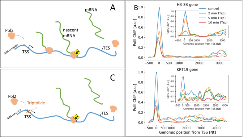
Figure 1: Biological processes and data. A) Simplified diagram of mRNA synthesis. PolII molecules bind to the DNA upstream of transcription start site (TSS) and moves downstream towards the transcription end site (TES), where it is released along with the synthesized mRNA. In certain genomic regions (indicated by a dangerous bend sign), PolIIs slow down. B) ChIP-seq experiments yield the relative abundance of PolII at each genomic position, here illustrated for H3-3B (top) and KR19 (bottom) genes; insets show the Spt5-bound PolII abundances for the same genes. C) In the presence of triptolide, transport is blocked upstream of TSS, while transcriptional engaged PolII are allowed to complete elongation; this is reflected in the ChIP-seq profiles obtained 2, 5, and 10 minutes after treatment (also in B).

Other methods available to study the pausing include but are not limited to NET-seq, where nascent mRNA chunks associated with immunoprecipitated PolII complexes are isolated and sequenced Nojima2015 , GRO-seq, where RNAs recently transcribed only by transcriptionally-engaged PolIIs are sequenced Core2008 , and PRO-seq, which is similar to GRO-seq but reaches single-nucleotide resolution Kwak2013 . The evidences of PolII transport are particularly clear in time-course experiments, where sequencing data are collected over time following a perturbation. As an example, time-variant PRO-seq has been suggested to estimate pausing times in key peak regions Zhang2021 . A classical way to perturb these molecular dynamics is inhibiting the initiation by treating the cells with triptolide (Trp), which is a highly specific drug that blocks initiation Jonkers2014 ; Erickson2018 . This permits the PolII already engaged in transcription to progress further downstream the gene while new PolIIs are prevented to attach, thus freeing upstream genomic regions as the run-on time progresses (Fig. 1 C). Our approach consists of using the read profiles $y$ as functions of $x$, collected at fixed run-on times $t_{1}$, $t_{2}$, $t_{3}$, and $t_{4}$ after treatment, to infer the dynamics. While Trp inhibits new initiation, poised PolII upstream the TSS can still pass through it, enter the gene template, and perform elongation immediately after Trp treatment Jonkers2014 ; Erickson2018 . To account for this, we also perform inference over Spt5 ChIP-seq data, where the poised polymerases are masked while those bound are detected Erickson2018 .

These types of experiments reveal the presence of a flux of PolIIs, which is the signature of the non-equilibrium physics involved in the elongation process. The profile $y^{*}$ observed prior to the treatment corresponds to a non-equilibrium stationary state (NESS). Disrupting initiation with Trp yields a transient state, which evolves from $y^{*}$ until it settles down to a new NESS.

II.2 Mathematical model

The transport of particles on a one dimensional lattice is a well-studied problem in mathematics and physics. Its basic features are captured by the asymmetric simple exclusion process (ASEP) Spitzer1970 , which defines the stochastic dynamics of interacting particles on a discrete lattice, which we take here to be a one-dimensional chain with open boundary conditions. Let the total number of lattice sites be $N$. The state of each site $i$, $1\leq i\leq N$, is characterized by the occupation number $n_{i}$ such that $n_{i}=0$ if the site is empty and $n_{i}=1$ if it is occupied by a particle. The evolution proceeds in continuous time. A particle on site $i<N$ hops rightward into the site $i+1$ with rate $p_{i}$, the transition being successful only if the site $i+1$ is empty. Similarly, a particle on site $i>1$ hops leftward into $i-1$ with rate $q_{i}$, if the site $i-1$ is empty. Further, particles on the left (right) boundary site $i=1$ ($i=N$) leave the lattice at rate $q_{1}$ ($p_{N}$), while particles are injected in the same boundary site at rate $p_{0}$ ($q_{N+1}$) if the site is empty. The constraint that a jump can occur only if the target is empty prevents the accumulation of more than one particle on a site and is generically referred to as the exclusion rule. This rule allows particle collision, which causes congestion when the particle density is sufficiently high and permits phase transitions between a low density, high density, and a maximum current phase even if the systems is one dimensional Chou2011 . Interestingly, based on theoretical considerations, it has been suggested that traffic-like congestion of PolIIs is important in transcription Klumpp2008 ; Cholewa-Waclaw2019 ; Tripathi2009 .

While the ASEP was originally proposed to model biopolymerization on on nucleic acid templates MacDonald1968 ; MacDonald69 , this and related models have been more recently applied to diverse problems, including protein translation Zia2011 ; Szavits-Nossan2018 ; Erdmann-Pham2019 , but also, e.g., molecular motors Lipowsky2001 and pedestrian and vehicle traffic Chowdhury2000 . Applications to transcription incorporating disordered dynamics and obstacles (e.g., Wang2014 ; Waclaw2019 ) were also proposed. ASEP’s theoretical appeal is due to its analytical results representative of a large class of models Kardar1986 ; Bertini1997 and a convenient mean-field treatment that yields the exact stationary solution Derrida1993 . In the context of transcription, particles entering site $1$, moving along the chain, and exiting from site $N$ correspond to initiation, elongation, and termination, respectively. In our setting, the lowest values of $p_{i}$ correspond to genomic locations were elongation slows down.

The dynamics of the expected occupation of a single site $i$ in the bulk are governed by the lattice continuity equation

$$\frac{d}{dt}\mathbb{E}(n_{i}(t))=J^{\mathrm{left}}(t)-J^{\mathrm{right}}(t),$$ (1)

$0<i<N$, where $\mathbb{E}$ denotes expectation value and $J^{\mathrm{left}}(t)$ and $J^{\mathrm{right}}(t)$ are the average flux of particles from site $i-1$ to site $i$ and from site $i$ to site $i+1$, respectively. These are subject to the exclusion rule and therefore obey

$$J^{\mathrm{left}}(t) =p_{i-1}\mathbb{E}(n_{i-1}(t)(1-n_{i}(t)))$$ (2)

$$-q_{i}\mathbb{E}(n_{i}(t)(1-n_{i-1}(t))),$$

$$J^{\mathrm{right}}(t) =p_{i}\mathbb{E}(n_{i}(t)(1-n_{i+1}(t)))$$

$$-q_{i+1}\mathbb{E}(n_{i+1}(t)(1-n_{i}(t))).$$

In order to exactly solve these dynamics, second-order moments such as $\mathbb{E}(n_{i}(t)n_{i+1}(t))$ need to be known. Under independence assumption, these moments are factorised, which in our case amounts to replacing equations (1)–(2) with

$$\frac{d}{dt}\phi_{i}(t) =p_{i-1}\phi_{i-1}(t)(1-\phi_{i}(t))-p_{i}\phi_{i}(t)(1-\phi_{i+1}(t))$$ (3)

$$+q_{i+1}\phi_{i+1}(t)(1-\phi_{i}(t))-q_{i}\phi_{i}(t)(1-\phi_{i-1}(t)),$$

where we used $\phi_{i}(t):=\mathbb{E}(n_{i}(t))$ to lighten the notation. In other words, equations (3) define the so-called mean-field dynamics of the asymmetric exclusion process, which are known to approximate well the true dynamics in many contexts, predict crucial features such as dynamical phase-transitions, and ease mathematical treatment Derrida1993 ; Chou2011 ; Lazarescu2015 . With open boundaries,

$$\begin{aligned} \frac{d}{dt}\phi_{1}(t)&=p_{0}\,(1-\phi_{1}(t))-p_{1}\phi_{1}(t)(1-\phi_{2}(t))\\ &-q_{1}\phi_{1}(t)+q_{2}\phi_{2}(t)(1-\phi_{1}(t)),\end{aligned}$$ (4)

$$\begin{aligned} \frac{d}{dt}\phi_{N}(t)&=p_{N-1}\phi_{N-1}(t)(1-\phi_{N}(t))-p_{N}\phi_{N}(t)\\ &+q_{N+1}\,(1-\phi_{N}(t))-q_{N}\phi_{N}(1-\phi_{N-1}).\end{aligned}$$ (5)

To match the available data that is coarse grained (Fig. 1 B), instead of considering particles individually we rely on their hydrodynamics description, which is obtained as follows. We assume Euler scaling with constant $a$ and let $a\to 0,N\to\infty$, with $L:=Na$ held finite. We define the functions $\varrho:\mathbbm{R}^{2}\to\mathbbm{R}^{+}_{0}$, $\tilde{p}:\mathbbm{R}\to\mathbbm{R}^{+}_{0}$, and $\tilde{q}:\mathbbm{R}\to\mathbbm{R}^{+}_{0}$ such that they are analytic and bounded on $]0,L[\times]0,\infty[$, $]0,L[$, and $]0,L[$, respectively, and

$$\phi_{i}(t) =\varrho((i-1)\,a,t),$$ (6)

$$a\,p_{i} =\tilde{p}((i-1)\,a),$$

$$a\,q_{i} =\tilde{q}((i-1)\,a).$$

We further assume that the left and right jump rates satisfy $\tilde{q}(x)=b\,\tilde{p}(x)$, $\forall x\in[0,L]$, with $0\leq b<1$, where $b$ governs the relative strength of the non-equilibrium driving forces. The case $b=0$ corresponds to a totally asymmetric exclusion process (TASEP), while the limit case $b=1$ corresponds to the symmetric exclusion process. Intermediate values $0<b<1$ correspond to settings where the particles can jump in both directions, but are driven rightwards on average. A continuum-limit counterpart of equations (2), as derived in references Harris2004 ; Stinchcombe2011 , is

$$J(x,t)=\tilde{p}(x)\varrho(x-a/2,t)(1-\varrho(x+a/2,t))-\tilde{q}(x)\varrho(x+a/2,t)(1-\varrho(x-a/2,t)),$$ (7)

which, using first-order Taylor expansion, yields

$$J(x,t)\approx(\tilde{p}(x)-\tilde{q}(x))\varrho(x,t)(1-\varrho(x,t))-\frac{a}{2}(\tilde{p}(x)+\tilde{q}(x))\frac{\partial}{\partial x}\varrho(x,t).$$ (8)

To lighten the mathematical notation, we define the two quantities

$$\lambda(x) :=(\tilde{p}(x)-\tilde{q}(x))=\tilde{p}(x)(1-b),$$ (9)

$$\nu(x) :=\frac{a}{2}(\tilde{p}(x)+\tilde{q}(x))=\frac{a}{2}\tilde{p}(x)(1+b);$$

their ratio is constant in $x$, viz., ${\nu(x)}/{\lambda(x)}={a}/{2}\,(1+b)/(1-b)$, which equals $a/2$ in the totally asymmetric case.

Substituting (8)–(9) into the continuity equation

$$\frac{\partial}{\partial t}\varrho(x,t)=-\frac{\partial}{\partial x}J(x,t),$$ (10)

which is the hydrodynamics limit of equation (1), gives the non-linear partial differential equation

$$\frac{\partial}{\partial t}\varrho(x,t)=-\frac{\partial}{\partial x}\Big{\{}\lambda(x)\varrho(x,t)(1-\varrho(x,t))-\nu(x)\frac{\partial}{\partial x}\varrho(x,t)\Big{\}},$$ (11)

which can be linearised to

$$\frac{\partial}{\partial t}u(x,t)=\frac{\tilde{p}(x)}{2}\Big{\{}{a^{2}}(1+b)\frac{\partial^{2}}{\partial^{2}x}u(x,t)\\ -\frac{(1-b)^{2}}{1+b}u(x,t)\Big{\}}$$ (12)

by means of a generalisation of the Cole-Hopf transform (Appendix A and references Hopf1950 ; Cole1951 ; Harris2004 ).

In transcription, the particle flux is left to right. While PolIIs can backtrack few Nts under certain circumstances Nudler1997 ; Julicher1998 ; Wang2009 , this phenomenon is overall minor and is not observable at our ChIP-seq resolution. Therefore, we assume $b=0$ and focus on the inference of the net forward rate profile $\tilde{p}(x)$. For simplicity we we also set $a=1$, arguing that our considerations remain valid with such a choice. The required boundary values $\varrho(0,t)$, $\varrho(L,t)$, and $\varrho(x,0)$, and the numerical scheme used to integrate equation (12) are detailed in Appendices A and B.

Integrating equation (11) with boundary conditions analogous to equations (4)–(5) and initial density $\varrho(x,0)>0$ yields a NESS for large $t$, characterised by a non-vanishing average flux and a density profile $\varrho^{*}(x)$ which is invariant in time. Setting the latter as initial condition and further integrating with no inward particle flux ($p_{0}=q_{N}=0$) produces a transient state that mimics the evolution of the PolII profile after Trp treatment until the density profile vanishes. This is illustrated, for a choice of boundary values and jump rate profile, in Fig. 2, which also includes the result of the inference process described in the next subsections.

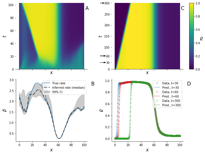
Figure 2: Simulation study. A) A non-equilibrium stationary state (NESS) of profile $\varrho^{*}(x)$ is obtained integrating the hydrodynamic TASEP with open boundaries, initial density profile $\varrho(x,0)=0.5$ $\forall x\in[0,L]$, and chosen rate profile (solid line in (B)). B) True rate profile (solid line) and inferred rate profile (dash-dot line); the shaded area is $99\%$ credible interval (CI). C) Integrating the same dynamics with initial profile $\varrho^{*}(x)$ and no-influx boundary conditions show that the density decreases in proximity of the left-boundary, similar to ChIP-seq readings followed by Trp treatment; the density profiles corresponding to times $30$, $60$, and $300$ and used for inference are marked by arrows. D) The posterior predictive samples (solid lines) are in excellent agreement with the extracted density profiles (cross markers); the posterior predictive dispersion is of the order of the line width, see also Fig. S3.

II.3 Bayesian framework

We fit the model to real-world data by means of a Bayesian approach, leveraging its ability to explicitly encode prior hypotheses about the quantities we wish to infer gelman2013bayesian . We are interested in the forward rate profile $\tilde{p}$. As this is required to be analytic and non-negative, it is convenient to assume a Gaussian process (GP) Rasmussen2006 functional prior on a latent variable $f$ and induce a prior on $\tilde{p}$ using a sigmoid link function of $f$, such that $\tilde{p}=\tilde{p}_{\mathrm{max}}/(1+\exp(-f))$, which further imposes an upper bound $\tilde{p}_{\mathrm{max}}$ to $\tilde{p}$. The GP prior here defines a distribution over real valued $C^{1}$ functions in $\mathbb{R}$, where any finite set of function evaluations $f(x)$ has multivariate normal distribution with mean $m$ and covariance kernel $k(x,x^{\prime};\sigma^{2}_{f},l)=\sigma^{2}_{f}\exp(-(x-x^{\prime})^{2}/(2\,l^{2}))$, $x,x^{\prime}\in\mathbb{R}$. In practice, the GP is evaluated at the positions $x_{i}$, $i=1,\ldots,\mathsf{n}$, where is it equivalent by definition to $\mathbf{f}\sim\mathcal{N}(m,\mathbf{K})$, a multivariate normal random variable with mean $m$ and covariance matrix $\mathbf{K}(\sigma_{f},l)$ induced by the kernel.

The observations are organised into a collection of values $\mathbf{y}=\{y_{ij}\}_{i=1,2,\ldots,\mathsf{n},j=1,2,\ldots,\mathsf{t}}$, where the subscripts indicate that an observation is taken at position $x_{i}$ and time $t_{j}$. As the values of $x_{i}$ do not necessarily coincide with the bin centers of ChIP-seq data, we used simple linear interpolation to estimate the data at intermediate coordinates. We assume that the observed values depend on a multiplicative factor and also include an additive error term $\epsilon\sim\mathcal{N}(0,\sigma_{\epsilon})$. This can be written in terms of the equation $\kappa y_{ij}=\varrho(x_{i},t_{j})+\epsilon$, where $\kappa$ is the inverse of the amplification factor. The likelihood $P(\mathbf{y}|\mathbf{f},\sigma_{\epsilon},\kappa)$ satisfies

$$\log P(\mathbf{y}|\mathbf{f},\sigma_{\epsilon},\kappa)=-\frac{1}{2\sigma^{2}_{\epsilon}}\sum_{i=1}^{\mathsf{n}}\sum_{j=1}^{\mathsf{t}}(\varrho(x_{i},t_{j};\mathbf{f})-\kappa y_{ij})-\frac{n}{2}\log(2\pi\sigma^{2}_{\epsilon}),$$ (13)

where we made explicit that $\varrho$ depends on $\mathbf{f}$. For the hierarchical parameters $(m,\sigma_{\epsilon},\kappa,\sigma_{f},l)=:\theta$ we assume a scaled sigmoid Gaussian prior probability $P(m,\sigma_{\epsilon},\kappa,\sigma_{f},l)$ such that

$$\theta=\theta_{\mathrm{min}}+\frac{(\theta_{\mathrm{max}}-\theta_{\mathrm{min}})}{1+\exp(-\xi)},\qquad\xi\sim\mathcal{N}(\mu_{\xi},\mathbbm{1}\sigma_{\xi}),$$ (14)

where $\theta_{\mathrm{min}}:=(m_{\mathrm{min}},{\sigma_{\epsilon}}_{\mathrm{min}},\kappa_{\mathrm{min}},{\sigma_{f}}_{\mathrm{min}},l_{\mathrm{min}})$, $\theta_{\mathrm{max}}:=(m_{\mathrm{max}},{\sigma_{\epsilon}}_{\mathrm{max}},\kappa_{\mathrm{max}},{\sigma_{f}}_{\mathrm{max}},l_{\mathrm{max}})$, and $(\mu_{\xi},\sigma_{\xi})$ are referred to as hyperparameters. Prior distributions are chosen to pull MCMC samples away from inappropriate results that are consistent with the likelihood but would not be consistent with domain knowledge gelman2013bayesian . By using scaled sigmoid Gaussian prior probability bounded by $\theta_{\mathrm{min}}$ and $\theta_{\mathrm{max}}$, we only search for solutions constrained in an appropriate interval Tegner2019 . By virtue of the Bayes theorem the joint posterior probability for $\theta$ and $\mathbf{f}$ satisfies

$$P(\mathbf{f},m,\sigma_{\epsilon},\kappa,\sigma_{f},l|\mathbf{y})\propto P(\mathbf{y}|\mathbf{f},\sigma_{\epsilon},\kappa)P(\mathbf{f}|m,\sigma_{f},l)P(m)P(\sigma_{\epsilon})P(\kappa)P(\sigma_{f})P(l),$$ (15)

which we draw random samples from by Markov chain Monte Carlo (MCMC) sampling, more specifically block Gibbs sampling with elliptical slice sampling at each block Murray2010 ; Tegner2019 (Appendix C). Equation (15) expresses the distribution of parameters given the observed data $\mathbf{y}$ and completes the definition of the model. It is worth noting that evaluating the likelihood also requires computing $\varrho$ by integrating equation (11) with initial condition $\varrho(x,0)=\kappa\,y^{*}(x)$, $\forall x\in[0,L]$.

III Results

We first consider simulated data from a given profile of length $L=100$ obtained from GP draw with parameters $(l,\sigma_{f},m,\tilde{p}_{\mathrm{max}})=(7.32,0.67,0.29,3)$. We integrate the dynamics with NESS initial profile (obtained by fixing the boundary conditions to $\varrho(0,t)=\varrho(L,t)=0.5$, $\forall t$ ) and no-influx boundary conditions (Fig. 2 A-B). The chosen rate profile shows a local minimum close to the left boundary, which yields a minor local perturbation in the density, and a global minimum around $x\approx 60$, whose effect propagates along the lattice and acts as a major bottleneck, which separates a low density phase downstream from a high-density phase upstream. These minima correspond to regions where particles slow down or pause for an exponentially distributed amount of time. As the particles leave the system through the right boundary and are not replenished by the influx through the left boundary, the region upstream the bottleneck is emptied by a reverse wave front.

For the purpose of testing whether we are able to recover the rate profile from time-course observations, we extract density profiles $\mathbf{y}$ at times $(t_{1},t_{2},t_{3})=(30,60,300)$ and set the hyperparameters $\theta_{\mathrm{min}}$, $\theta_{\mathrm{max}}$, and $(\mu_{\xi},\sigma_{\xi})$ to $(0,0,0.8,0,0)$, $(2,10,1.2,1,10)$, and $(0,1)$, respectively. With these settings and data, we generated $10^{4}$ MCMC samples targeting the posterior (15), discarding the first $2\times 10^{3}$ as burn-in, demonstrating that the fitting procedure is able to capture the location of both the major and minor minima of the generative model, as well as the overall elongation rate (Fig. 2 B). It is worth noting that the integrated density profile in Fig. 2 C and D displays a very small effect of the first local minimum (minor dip, captured only by time-course profiles at $t_{1}$ and $t_{2}$); this is reflected in relatively wide credible intervals for the inferred rate profile (grey ribbon in Fig. 2 B). On the other hand, the rate at the bottleneck is inferred with very high confidence. The covariance hyperparameters $l$ and $\sigma_{f}$ control how quickly the rate changes over $x$; these were slightly misestimated to 6.86 (95%CI 4.63–7.16) and 0.76 (95%CI 0.75–0.82), respectively, thus suggesting that increased wobbling in the rate profile is tolerated; minor patterns in the rate profile are in fact smoothed out and are essentially not identifiable in the density profiles obtained by integration (see Fig. S3). The difficulty of sampling covariance hyperparameters is also addressed, e.g., in Tegner2019 . The predicted transient density profiles at $t=30,60,300$ also are in very good agreement with the input data (Fig. 2 D; in fact, all sampled rate profiles yield similar time-course density profiles despite wide CIs in certain regions (see also Fig. S3).

Applying this method to real-world data requires setting the value of $\tilde{p}_{\mathrm{max}}$ to an upper limit of prior expectations on the elongation rate. As this has been estimated at around $2\times 10^{3}$ Nt/min in previous studies Jonkers2014 , we set $\tilde{p}_{\mathrm{max}}=6\times 10^{3}$ Nt/min as an arguably safe upper bound. Literature results can be also used to set bounds on the prior for $\kappa$, which regularises the estimation problem Rasmussen2006 . From cultured human cell lines, the total number $\mathrm{P}$ of bound PolII molecules per cell is estimated to be between $\mathrm{P}_{\mathrm{min}}=11\times 10^{5}$ and $\mathrm{P}_{\mathrm{max}}=18\times 10^{5}$ Kimura1999 . This is related to the total number $Y$ of ChIP-seq counts by $\mathrm{P}=\kappa\,Y$. Based on these heuristic considerations, we set $\kappa_{\mathrm{min}}=\mathrm{P}_{\mathrm{min}}/Y$ and $\kappa_{\mathrm{max}}=\mathrm{P}_{\mathrm{max}}/Y$. All remaining hyperparameters were set identical to the previous simulation experiment.

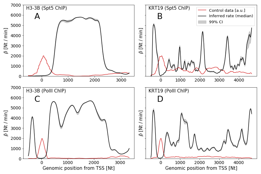
Figure 3: Inferred rate profiles from Spt5 ChIP-seq (A-B) and PolII ChIP-seq (C-D) for genes H3-B3 (A-C) and KRT19 (B-D) (black lines are posterior medians, shaded area are 99% credible intervals), with the latter gene showing a distinctive jagged profiles. Both genes show the lowest rates in proximity of the transcription starting site (TSS). Red lines are unperturbed ChIP-seq signals in arbitrary units (a.u.).

The results from different genes show a variety of rate profiles which share similar patterns (Fig. 3). The most important observation is that, in all genes considered, the rates vary strongly with the genomic position, with local minima corresponding to regions where PolIIs slow down or pause. In order to look for average patterns, it is desirable to aggregate data from all genes. As genes have different lengths (which in our sample range from 16,680 to 59,880 Nts), we stretch all the rate profiles in the region from TSS+1000 to TES-1000 Nts to the same support length and then average over the genes at each position. This yields the summaries illustrated in Fig. 4 which we refer to as metagene rates and are akin to the so-called metagene profiles JolyBeauparlant2016 .

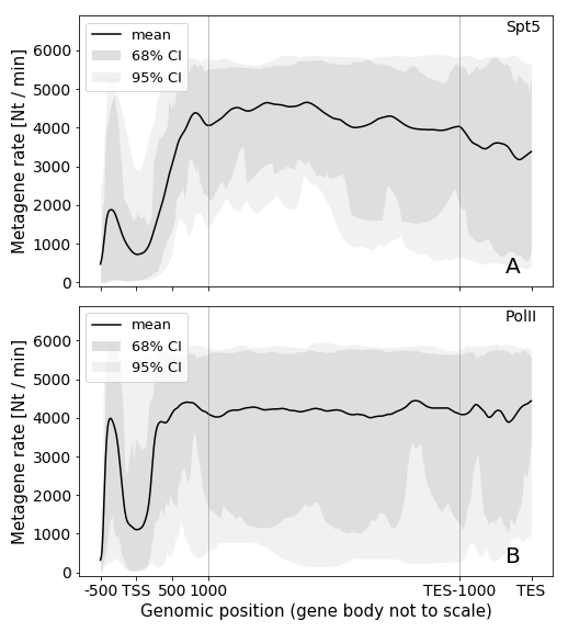
Figure 4: Metagene rates from PolII ChIP-seq (A) and Spt5 ChIP-seq (B) data. By construction, the metagene analysis conserves the length scale only in proximity of TSS and TES. Upstream of TSS the Spt5 ChIP-seq yields lower average rate than PolII ChIP-seq, as this assay does not detect PolII poised to move downstream.

Rates are typically lower near the TSS than in the gene body, where elongation approaches its highest rate. The behaviour in proximity of the TES is less definite, with rates varying several fold among the different genes. At the TSS the rate typically dips down consistently with the presence of strong and widespread pausing in this region. Further downstream in the gene body the rate increases to its highest average value. While the dip is evident in both Spt5 and PolII results, it is worth noting that upstream the TSS the average rate inferred from PolII data is higher than that from Spt5. We argue that this difference is due to the fact the former also include poised PolIIs which are not strongly bound to the template and can quickly move towards the TSS before being engaged in transcription. A by-product of the fitting procedure is the estimate of the occupation density $\varrho(x,t)=\kappa\,y(x,t)$, as illustrated in Fig. 2 D for the simulation experiment and Figs. 5, S4, S5, and S6 for selected genes. The predicted densities are typically very low (total predicted number of PolIIs in a gene is in the order of $10^{-1}$), thus suggesting that crowding and congestion of PolIIs into a gene might not be substantial even proximal to rate minima.

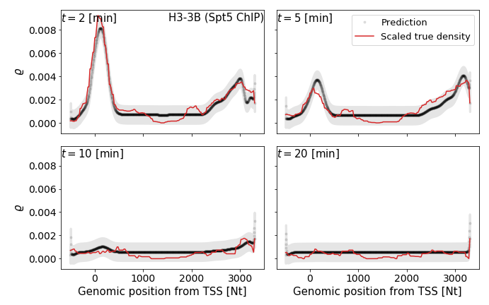
Figure 5: Predicted density profiles for gene H3-3B from Spt5 ChIP-seq $2$, $5$, $10$, and $20$ minutes after Trp treatment as samples from posterior predictive distribution. Grey area is 95% credible interval due to noise model.

IV Discussion

We developed a general Bayesian framework to study the dynamics of a one-dimensional transport model given time-resolved density profiles. The general problem addressed here is the identification of the PDE parameters that best describe data as a subset of the true PDE solution (see, e.g., Rudy2017 ; Raissi2019 ; Berg2019 ; Tegner2019 and references therein). We focused on the hydrodynamic TASEP with smoothly-varying jump rates (which are the parameters to be inferred) as a paradigmatic and well-characterised model of transport. By means of its application to ChIP-seq time-course data, we inferred the rate of PolII elongation as a function of the genomic position in selected genes. This rate is not constant but varies within the gene body. It typically dips down nearby the TSS, confirming widespread pausing in this region, while in the bulk the rate also varies between genes. Low predicted densities suggest that the pausing did not cause congestion or crowding. This is an important observation, as factor crowding has been experimentally observed and associated with regulated gene expression in synthetic and mammalian cell systems Tan2013 ; Hnisz2017 ; Plys2018 ; Boija2018 ; Cavallaro2019 . Our analysis supports the view that this phenomenon does not happen between PolIIs bound to the gene but likely occurs in suspension in the nucleoplasm, as described, e.g., in Papantonis2013 ; Boehning2018 ; Plys2018 ; Cavallaro2019 ; Cramer2019 ; Wei2020 .

The inference here is complicated by the high dimensionality of the parameter space (which grows as the genes’ length increases). We addressed this by assuming a Gaussian process latent prior for the jump-rate profile and using elliptic slice sampling as an appropriate MCMC algorithm. The sampling requires multiple evaluations of the likelihood of equation (13). This in turns requires numerically integrating equation (11), which is also slower in longer genes (require larger integration grids, see Appendix B).

This study of molecular dynamics is also subject to limitations. While ChIP-seq is a widely-used assay to quantify the abundances of DNA-bound PolII, studies suggest that it has limited resolution (between 150-300 Nts) and might be subject to technical issues Park2009 . Most importantly ChIP-seq profiles are obtained from the aggregation of sequencing reads from many cells, which hides variation within the cell population. The transcription of mRNA is a very complex process and it may be interesting to include features not encoded in the model used for this study. Other TASEP variants, such as those incorporating non-Markovian jump dynamics Khoromskaia2014 ; Concannon2014 or Langmuir kinetics Parmeggiani2004 , are relevant for the modelling of PolII recycling and its early detachment from DNA Steurer2018 ; Cavallaro2019 . An assumption of the TASEP is that particles stay in a site for an exponentially distributed waiting time. Variants of TASEP in which defects appear and disappear randomly on any site (and thus slow down the movement of particles or even block it completely) have been introduced in physics literature and can account for occasionally long pausing times Wang2014 ; Waclaw2019 (see also Concannon2014 ; Khoromskaia2014 ), with defect dynamics representing the effects of pausing and elongation factors. Modelling advancements that combine the site-specific pausing with long pausing times and extended particle size, supplemented by an appropriate inference scheme such as the one presented here, would be an important additional potential area for research and application. Potential extensions of our work also include estimation of the parameters that encode the system’s size and asymmetry ($a$ and $b$, respectively) and the boundary values. Statistical mechanics literature is rich in quantitative studies of TASEPs with particles that occupy more than one lattice site Shaw2003 ; Schonherr2004 ; Schonherr2005 , some generalized to include site-dependent elongation rates or localised defects Shaw2004 ; Shaw2004a ; Dong2007 ; Erdmann-Pham2019 . These studies have been used to describe protein translation and could be useful to predict PolII-size effects in gene expression, although, with genes much longer than PolIIs, ChIP-seq limited resolution, and very low PolII coverage density, the observable correction would arguably be minor. In fact, including more features plausibly requires sequencing assays of higher resolution than ChIP-seq and comes at the cost of increased computational burden and decreased tractability. Conversely, the chosen TASEP with smoothly-varying jump rates is simple and yet is able to reveal PolII elongation slowing down and speeding up at certain genomic locations. Due to its generality, our approach also serves as a template for future studies seeking to shed light on complex transport phenomena.

Materials and Methods

Spt5 and PolII ChIP-seq data mapped to the hg19 University of California at Santa Cruz human genome were downloaded from Gene Expression Omnibus (GEO, http://www.ncbi.nlm.nih.gov/geo), accession number GSE117006. We filtered the list of genes from the reference genome to only contain those with unique gene symbols on chromosomes 1–22 and X, thus excluding alternatively spliced genes. Hg19 gene coordinates were flanked 500 Nts upstream the TSS in order to include poised PolII. The 20 non-overlapping genes with the highest coverage of Spt5 ChIP-seq reads were selected. All simulation codes are written in c++ and Python (v3.7.1), with the PDE solver using Numba JIT compiler (v0.41.0) Lam2015 (https://github.com/mcavallaro/dTASEP-fit).

Author contributions

Conceptualization MC DH RD; Data curation MC DH; Formal analysis MC RD; Investigation MC; Software MC YW RD; Writing – original draft MC; Writing – review & editing MC DH RD.

Appendix A Cole-Hopf transform

Let us define a “height” variable $h(x,t)$ as follows:

$$\varrho(x,t)=:\frac{\partial}{\partial x}h(x,t)+\frac{1}{2}.$$ (16)

Substituting this into equation (11) of the main text yields

$$\frac{\partial}{\partial t}\frac{\partial}{\partial x}h(x,t)=-\frac{\partial}{\partial x}\left\{\lambda(x)\left(\frac{\partial}{\partial x}h(x,t)+\frac{1}{2}\right)\left(\frac{1}{2}-\frac{\partial}{\partial x}h(x,t)\right)-\nu(x)\frac{\partial^{2}}{\partial^{2}x}h(x,t)\right\}$$ (17)

and integrating over $x$ gives

$$\frac{\partial}{\partial t}h(x,t)=-\lambda(x)\left(\frac{\partial}{\partial x}h(x,t)+\frac{1}{2}\right)\left(\frac{1}{2}-\frac{\partial}{\partial x}h(x,t)\right)+\nu(x)\frac{\partial^{2}}{\partial^{2}x}h(x,t)+f(t),$$ (18)

which is a noiseless version of the paradigmatic growth model studied by Kardar, Parisi, and Zhang Kardar1986 up to an arbitrary integration function $f(t)$ constant in $x$.

This equation is linearised by means of the transformation

$$h(x,t)=:\frac{a}{2}\frac{1+b}{1-b}\ln u(x,t)+F(t),$$ (19)

which obviously implies

$$\frac{\partial}{\partial x}h(x,t)=\frac{a}{2}\frac{1+b}{1-b}\frac{u_{x}(x,t)}{u(x,t)}.$$ (20)

We refer to $u(x,t)$ as the “field”.

Merely substituting (19) into equation (18) and choosing $F(t)$ to remove the term $f(t)$ yields

$$\frac{a}{2}\frac{1+b}{1-b}\frac{u_{t}(x,t)}{u(x,t)}=-\left\{\lambda(x)\left[\frac{1}{4}-\left(\frac{a}{2}\frac{1+b}{1-b}\frac{u_{x}(x,t)}{u(x,t)}\right)^{2}\right]-\nu(x)\frac{a}{2}\frac{1+b}{1-b}\frac{\partial}{\partial x}\frac{u_{x}(x,t)}{u(x,t)}\right\},$$ (21)

$$\frac{a}{2}\frac{1+b}{1-b}\frac{u_{t}(x,t)}{u(x,t)}=\\ -a\tilde{p}(x)\left\{\left[\frac{(1-b)}{4}-\frac{a^{2}}{4}\frac{(1+b)^{2}}{(1-b)}\frac{(u_{x}(x,t))^{2}}{u^{2}(x,t)}\right]-\frac{a^{2}}{4}\frac{(1+b)^{2}}{1-b}\left(\frac{u_{xx}(x,t)}{u(x,t)}-\frac{(u_{x}(x,t))^{2}}{u^{2}(x,t)}\right)\right\},$$ (22)

$$\frac{1}{2}\frac{1+b}{1-b}\frac{u_{t}(x,t)}{u(x,t)}=\\ -\tilde{p}(x)\left\{\frac{(1-b)}{4}-\cancel{\frac{a^{2}}{4}\frac{(1+b)^{2}}{(1-b)}\frac{(u_{x}(x,t))^{2}}{u^{2}(x,t)}}-\frac{a^{2}}{4}\frac{(1+b)^{2}}{1-b}\frac{u_{xx}(x,t)}{u(x,t)}+\cancel{\frac{a^{2}}{4}\frac{(1+b)^{2}}{1-b}\frac{(u_{x}(x,t))^{2}}{u^{2}(x,t)}}\right\},$$ (23)

$$\frac{\partial}{\partial t}u(x,t)=\frac{\tilde{p}(x)}{2}\left\{{a^{2}}(1+b)\frac{\partial^{2}}{\partial^{2}x}u(x,t)-\frac{(1-b)^{2}}{1+b}u(x,t)\right\},$$ (24)

which, for the totally asymmetric case $b=0$, can be simplified to

$$\frac{\partial}{\partial t}u(x,t)=\frac{\tilde{p}(x)}{2}\left\{{a^{2}}\frac{\partial^{2}}{\partial^{2}x}u(x,t)-u(x,t)\right\}.$$ (25)

To the best of our knowledge, this parametrisation was first derived in reference Harris2004 . If $\tilde{p}(x)=p$, it is possible to incorporate a term $-a\,p\,(1-b)\,t/4$ in $F(t)$ to eliminate the second term on the right-hand side of equations (24) and (25), thus further simplifying these to diffusion equations.

Equation (24) preserves the full dynamics of equation (11) of the main text and is linear, thus it is easier to treat numerically than the latter. In the next sections we elucidate the numerical scheme for its integration for $b=0$.

We impose Dirichlet boundary conditions for $\varrho(x,t)$ at $x=0$ and $x=L$, i.e.,

$$\varrho(0,t) =\varrho_{\mathrm{left}}(t),$$ (26)

$$\varrho(L,t) =\varrho_{\mathrm{right}}(t),$$

$\forall t>0$, which implies Neumann conditions for the height $h(x,t)$:

$$h_{x}(x,t)|_{x=0} =\varrho_{\mathrm{left}}(t)-\frac{1}{2},$$ (27)

$$h_{x}(x,t)|_{x=L} =\varrho_{\mathrm{right}}(t)-\frac{1}{2},$$

and Robin (mixed) boundary conditions for the field $u(x,t)$:

$$(2\varrho_{\mathrm{left}}(t)-1)u(0,t)/a-u_{x}(x,t)|_{x=0} =0,$$ (28)

$$(2\varrho_{\mathrm{right}}(t)-1)u(L,t)/a-u_{x}(x,t)|_{x=L} =0.$$ (29)

Appendix B Numerical integration

The solution $u^{*}$ of equation (25) at the coordinates $(\mathsf{i}\,\Delta x,\mathsf{j}\,\Delta t)$ is approximated by $U_{\mathsf{j},\mathsf{i}}$ ($\mathsf{j}=0,1,\ldots,T$ and $\mathsf{i}=0,1,\ldots,\mathsf{N}$ with $\mathsf{N}=L/\Delta x$) which is computed using the forward Euler explicit iterative procedure

$$U_{\mathsf{j}+1,\mathsf{i}}=U_{\mathsf{j},\mathsf{i}}+P_{\mathsf{i}}\,\left[a^{2}\frac{U_{\mathsf{j},\mathsf{i}-1}-2U_{\mathsf{j},\mathsf{i}}+U_{\mathsf{j},\mathsf{i}+1}}{\Delta x^{2}}-U_{\mathsf{j},\mathsf{i}}\right]\Delta t,$$ (30)

where $P_{\mathsf{i}}=\tilde{p}(\mathsf{i}\,\Delta x)$. The approximated density $\rho_{\mathsf{j},\mathsf{i}}\approx\varrho(\mathsf{i}\Delta x,\mathsf{j}\Delta t)$ is recovered from $U_{\mathsf{j},\mathsf{i}}$ by means of the transformation

$$H_{\mathsf{j},\mathsf{i}} =\frac{a}{2}\,\ln U_{\mathsf{j},\mathsf{i}},$$ (31)

$$\rho_{\mathsf{j},\mathsf{i}} =\frac{1}{2}+\frac{H_{\mathsf{j},\mathsf{i}+1}-H_{\mathsf{j},\mathsf{i}-1}}{2\Delta x}.$$

Initial values $U_{0,\mathsf{i}}$, $\mathsf{i}=0,1,\ldots,\mathsf{N}$, are obtained by means of the discrete Cole-Hopf transform

$$U_{\mathsf{j},\mathsf{i}}=\exp\left(\sum_{\mathsf{k}=0}^{\mathsf{i}}\frac{1}{a}(2\rho_{\mathsf{j},\mathsf{k}}-1)\Delta{x}\right),$$ (32)

at $\mathsf{j}=0$ and given $\rho_{0,\mathsf{i}}$. We deal with the boundary conditions by introducing ghost grid points $(\mathsf{j},-1)$ and $(\mathsf{j},\mathsf{N}+1)$, with $\mathsf{j}=0,1,2,\ldots,T$), where the values of $U$ are determined according to the procedure detailed below.

We use a central difference formula to approximate the derivatives

$$u_{x}|_{x=0}(x,t) \approx\frac{U_{\mathsf{j},1}-U_{\mathsf{j},-1}}{2\Delta x},$$ (33)

$$u_{x}|_{x=L}(x,t) \approx\frac{U_{\mathsf{j},\mathsf{N}+1}-U_{\mathsf{j},\mathsf{N}-1}}{2\Delta x},$$ (34)

while $u(0,t)\approx U_{\mathsf{j},1}$ and $u(L,t)\approx U_{\mathsf{j},\mathsf{N}}$. Substituting into equations (28)–(29):

$$U_{\mathsf{j},-1} \approx U_{\mathsf{j},1}-2\Delta x[2\,\rho_{\mathsf{j},0}-1]\frac{1}{a}U_{\mathsf{j},0},$$ (35)

$$U_{\mathsf{j},\mathsf{N}+1} \approx\qquad+2\Delta x[2\,\rho_{\mathsf{j},\mathsf{N}}-1]\frac{1}{a}U_{\mathsf{j},\mathsf{N}}+U_{\mathsf{j},\mathsf{N}-1}.$$ (36)

The off-grid values $U_{\mathsf{j},-1}$ and $U_{\mathsf{j},\mathsf{N}+1}$ correspond to the ghost grid points and are eliminated by substitution from the recursion relations (30) at $\mathsf{i}=0$ and $\mathsf{i}=\mathsf{N}$, which we write for convenience:

$$U_{\mathsf{j}+1,0} =U_{\mathsf{j},0}+P_{0}\,\left[a^{2}\frac{U_{\mathsf{j},-1}-2U_{\mathsf{j},0}+U_{\mathsf{j},1}}{\Delta x^{2}}-U_{\mathsf{j},0}\right]\Delta t,$$ (37)

$$U_{\mathsf{j}+1,\mathsf{N}} =U_{\mathsf{j},\mathsf{N}}+P_{\mathsf{N}}\,\left[a^{2}\frac{U_{\mathsf{j},\mathsf{N}-1}-2U_{\mathsf{j},\mathsf{N}}+U_{\mathsf{j},\mathsf{N}+1}}{\Delta x^{2}}-U_{\mathsf{j},\mathsf{N}}\right]\Delta t.$$ (38)

The approximated second derivatives in the square brackets therefore are

$$\frac{U_{\mathsf{j},-1}-2U_{\mathsf{j},0}+U_{\mathsf{j},1}}{\Delta x^{2}}=\frac{L_{\mathsf{j}}\,U_{\mathsf{j},0}+2U_{\mathsf{j},1}}{\Delta x^{2}},\quad\mbox{with}\,L_{\mathsf{j}}=-2-2[2\,\rho_{\mathsf{j},0}-1]\Delta x\frac{1}{a},$$ (39)

and

$$\frac{U_{\mathsf{j},\mathsf{N}-1}-2U_{\mathsf{j},\mathsf{N}}+U_{\mathsf{j},\mathsf{N}+1}}{\Delta x^{2}}=\frac{2U_{\mathsf{j},\mathsf{N}-1}+R_{\mathsf{j}}\,U_{\mathsf{j},\mathsf{N}}}{\Delta x^{2}},\quad\mbox{with}\,R_{\mathsf{j}}=-2+2[2\,\rho_{\mathsf{j},\mathsf{N}}-1]\Delta x\frac{1}{a},$$ (40)

for the left and the right boundaries, respectively.

The recruitment of new PolII at the 5’ end of the gene is arrested upon chemical perturbation of the promoters with Trp. This is modelled by assuming that a PolII molecule at the leftmost site can leave its position, whilst no molecules can be injected. Therefore, in mean-field approximation, the average number of particles at the left boundary of the system obeys

$$\frac{d\phi_{0}(t)}{dt}=-p_{0}\phi_{0}(t)(1-\phi_{1}(t)),$$ (41)

whose hydrodynamic limit is approximated by

$$\frac{\partial}{\partial t}\varrho(0,t)\approx -a\,\tilde{p}(0)\varrho(0,t)(1-\varrho(0,t)-a\frac{\partial}{\partial x}\varrho(x,t)|^{+}_{x=0}).$$ (42)

with discretised iterative solution

$$\rho_{j+1,0}-\rho_{j,0} =-\Delta t\,a\,P_{0}\,\rho_{j,0}\left(1-\rho_{j,0}-a\frac{\rho_{j,1}-\rho_{j,0}}{\Delta x}\right),$$ (44)

$$\rho_{0,0} =\varrho_{L}(0),$$

$$\rho_{0,1} =\varrho(\Delta x,0).$$

Using equations (44) to iteratively update $L_{\mathsf{j}}$ in (39) yields open boundary conditions, which are used in the simulation experiments. The dynamics of the hydrodynamic limit approximate well the occupation density a TASEP with open boundaries on a large yet finite lattice ($N=600$) as illustrated in Fig. S1.

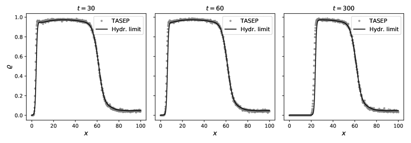
Figure S1: Comparison of the hydrodynamic solution (solid lines) and Monte Carlo simulation (Gillespie algorithm as update rule, ensemble size of $1000$) occupation density of a TASEP with open boundaries, lattice size $N=600$, and smoothly varying hopping rates (grey markers). Parameters and boundary conditions as in Fig. 2-D.

Sequencing data shows that, at the beginning of the flanked region upstream of the TSS, expression is very low and thus signal will remain constantly close to zero during the time course. The reads downstream the TES are also assumed to be constant within measurement errors, given that the Trp perturbation at the TSS does not propagate up until the TES in the longest time course. Based on this, we set fixed left and right boundary conditions. The grid constants $\Delta t$ and $\Delta x$ are chosen such that $\Delta t/\Delta x^{2}=1/\tilde{p}_{\mathrm{max}}$, which guarantees numerical stability at each grid point provided that $\tilde{p}(x)<\tilde{p}_{\mathrm{max}}$ $\forall x\in[0,L]$. The initial values over this grid at $\mathsf{j}=0$ are obtained from the binned read profile $y^{*}$ by means of linear interpolation.

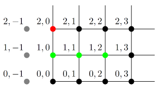
Figure S2: Evaluation of the discretised field $U$ at left-boundary grid nodes. The value at the red node is obtained from the values at the green nodes. Grey points are ghost grid nodes.

Appendix C MCMC sampling

In equation (15) of the main text, the posterior probability $P(\mathbf{f},m,\sigma_{\epsilon},\kappa,\sigma_{f},l|\mathbf{y})$ is expressed as proportional to the likelihood $P(\mathbf{y}|\mathbf{f},\sigma_{\epsilon},\kappa)$, multiplied by the latent GP prior $P(\mathbf{f}|m,\sigma_{f},l)$ times the prior $P(m,\sigma_{\epsilon},\kappa,\sigma_{f},l)$. The meanings of each parameter are summarised in Table S1.

Parameter	Prior	Description
$\tilde{p}$	$\tilde{p}_{\mathrm{max}}/(1+\exp(-\mathbf{f})),$ $\mathbf{f}\sim\mathcal{N}(m,\mathbf{K}(\sigma_{f},l))$	Rate profile, main target for inference and linked to a Gaussian process (GP) prior; evaluated at specific points, the GP is equivalent to a multivariate normal.
$m$	$m_{\mathrm{min}}+\frac{(m_{\mathrm{max}}-m_{\mathrm{min}})}{1+\exp(-\xi_{m})},\,\xi_{m}\sim\mathcal{N}(0,1)$	Location parameter (mean) of the GP prior.
$\sigma_{f}$	${\sigma_{f}}_{\mathrm{min}}+\frac{({\sigma_{f}}_{\mathrm{max}}-{\sigma_{f}}_{\mathrm{min}})}{1+\exp(-\xi_{f})},\,\xi_{f}\sim\mathcal{N}(0,1)$	Amplitude of the GP prior.
$l$	$l_{\mathrm{min}}+\frac{(l_{\mathrm{max}}-l_{\mathrm{min}})}{1+\exp(-\xi_{l})},\,\xi_{l}\sim\mathcal{N}(0,1)$	Characteristic length scale of the GP prior (as $l$ decreases, the GP varies more rapidly with $x$).
$\sigma_{\epsilon}$	${\sigma_{\epsilon}}_{\mathrm{min}}+\frac{({\sigma_{\epsilon}}_{\mathrm{max}}-{\sigma_{\epsilon}}_{\mathrm{min}})}{1+\exp(-\xi_{\epsilon})},\,\xi_{\epsilon}\sim\mathcal{N}(0,1)$	Standard deviation of normal measurement error.
$\kappa$	$\kappa_{\mathrm{min}}+\frac{(\kappa_{\mathrm{max}}-\kappa_{\mathrm{min}})}{1+\exp(-\xi_{\kappa})},\,\xi_{\kappa}\sim\mathcal{N}(0,1)$	Proportionality factor to convert ChIP-seq reads into occupation density.

Table S1: Target parameters for inference.

To sample from the posterior we used a blocked Gibbs sampling scheme where we recursively update the latent variable $\mathbf{f}$, the two covariance variables $l,\sigma_{f}$, and the three likelihood variables $m,\kappa,\sigma_{\epsilon}$, using the so-called elliptic slice sampler Murray2010 for each block.

In order to update $\mathbf{f}$ as a first block we parametrise the posterior such that $m$ is absorbed into the likelihood, i.e.,

$$P({\mathbf{f}}^{\prime},m,\sigma_{\epsilon},\kappa,\sigma_{f},l|\mathbf{y})\propto P(\mathbf{y}|{\mathbf{f}}^{\prime},m,\sigma_{\epsilon},\kappa)P({\mathbf{f}}^{\prime}|\sigma_{f},l)P(m)P(\sigma_{\epsilon})P(\kappa)P(\sigma_{f})P(l),$$ (45)

where ${\mathbf{f}}^{\prime}=\mathbf{f}-m$, and sample from the unnormalised conditional $P(\mathbf{y}|{\mathbf{f}}^{\prime},m,\sigma_{\epsilon},\kappa)P({\mathbf{f}}^{\prime}|\sigma_{f},l)$ with all hyperparameters $m$, $\sigma_{\epsilon}$, $\kappa$, $\sigma_{f}$, and $l$ held fixed.

Updating the second block $(l,\sigma_{f})$ is difficult as this is strongly correlated with $\mathbf{f}$. Hence we adopt another parametrisation, which consists of expressing the multivariate Gaussian random variable ${\mathbf{f}}^{\prime}$ as the deterministic function of $\bm{\nu}$

$${\mathbf{f}}^{\prime}(\bm{\nu},\sigma_{f},l)=\mathbf{L}\bm{\nu},$$ (46)

where $\mathbf{L}(\sigma_{f},l)$ satisfies $\mathbf{L}\mathbf{L}^{-1}=\mathbf{K}(\sigma_{f},l)$ (it can be computed from $\mathbf{K}$ using a Cholesky decomposition) and $\bm{\nu}\sim\mathcal{N}(0,\mathbbm{1})$ is independent of the other variables. This parametrisation incorporates all variables into the likelihood and results in the equivalent posterior

$$P(\bm{\nu},m,\sigma_{\epsilon},\kappa,\sigma_{f},l|\mathbf{y})\propto P(\mathbf{y}|{\mathbf{f}}^{\prime}(\bm{\nu},\sigma_{f},l),m,\sigma_{\epsilon},\kappa)P(\bm{\nu})P(m)P(\sigma_{\epsilon})P(\kappa)P(\sigma_{f})P(l).$$ (47)

For a given value of $({\mathbf{f}}^{\prime},l,\sigma_{f})$, $\nu$ is obtained as $\nu={\mathbf{L}(\sigma_{f},l)}^{-1}\,{\mathbf{f}}^{\prime}$. Hence with parameters ${\mathbf{f}}^{\prime},m,\kappa$, and $\sigma_{\epsilon}$ held fixed, we update $(\sigma_{f},l)$ with a sample from the unnormalised conditional $P(\mathbf{y}|{\mathbf{f}}^{\prime}(\bm{\nu},\sigma_{f},l),\kappa,\sigma_{\epsilon})P(\sigma_{f})P(l)$.

In the third step, given the values for ${\mathbf{f}}^{\prime}$, $l$, and $\sigma_{f}$, the likelihood hyperparameters $m$, $\sigma_{\epsilon}$, and $\kappa$ are updated by sampling from the unnormalised conditional $P(\mathbf{y}|{\mathbf{f}}^{\prime},m,\sigma_{\epsilon})P(m)P(\sigma_{\epsilon})P(\kappa)$. We refer the reader to Tegner2019 for more details. Posterior predictions are in very good agreement with time-course observations. Concentration of posterior-predictive samples around target data points can be appreciated by zooming in (Fig. S3).

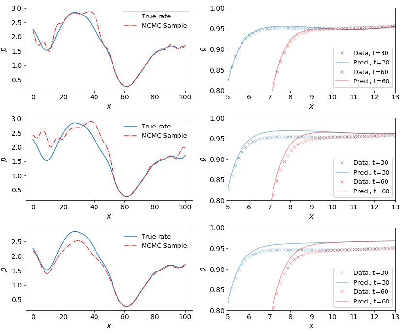
Figure S3: The rate profile samples sometimes have jagged profiles (left). The resulting density profiles are smoother than the corresponding rates and their dispersion around the input data profile can be appreciated by zooming in the plot of Fig. 2-D (right).

The model is weakly sensitive to changes in the rate profile except for the bottleneck minimum at $x\approx 60$, which is sampled with high confidence.

Appendix D Supplemental figures

Figs. S4, S5, and S6 illustrate the posterior predictive samples and the scaled ChIP-seq reads.

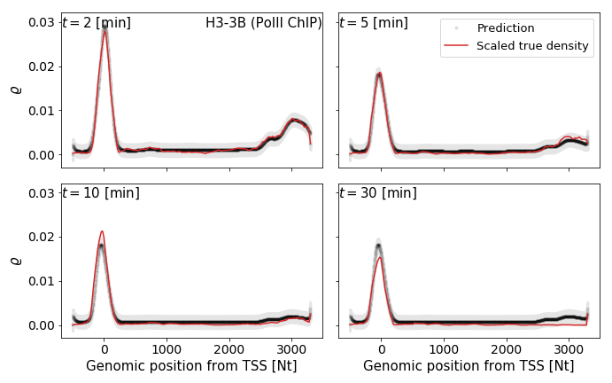
Figure S4: Predicted density profiles for gene H3-3B from PolII ChIP-seq, $2$, $5$, $10$, and $20$ minutes after Trp treatment. Markers are posterior predictive samples. Grey area is 95% credible interval due to noise model.

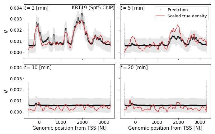
Figure S5: Predicted density profiles for gene KRT19 from Spt5 ChIP-seq. Figure keys as in Fig. S4.

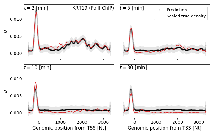
Figure S6: Predicted density profiles for gene KRT19 from PolII ChIP-seq. Figure keys as in Fig. S4.

References

- (1) Munsky B, Neuert G, van Oudenaarden A. Using Gene Expression Noise to Understand Gene Regulation. Science. 2012 apr;336(6078):183-7. doi:10.1126/science.1216379.
- (2) Rajala T, Häkkinen A, Healy S, Yli-Harja O, Ribeiro AS. Effects of Transcriptional Pausing on Gene Expression Dynamics. PLoS Comput Biol. 2010 03;6(3):1-12. doi:10.1371/journal.pcbi.1000704.
- (3) Jonkers I, Lis JT. Getting up to speed with transcription elongation by RNA polymerase II. Nat Rev Mol Cell Biol. 2015 mar;16(3):167-77. doi:10.1038/nrm3953.
- (4) Mayer A, Landry HM, Churchman LS. Pause & go: from the discovery of RNA polymerase pausing to its functional implications. Curr Opin Cell Biol. 2017 jun;46:72-80. doi:10.1016/j.ceb.2017.03.002.
- (5) Adelman K, Lis JT. Promoter-proximal pausing of RNA polymerase II: emerging roles in metazoans. Nat Rev Genet. 2012 sep;13(10):720-31. doi:10.1038/nrg3293.
- (6) Liu X, Kraus WL, Bai X. Ready, pause, go: Regulation of RNA polymerase II pausing and release by cellular signaling pathways. Trends Biochem Sci. 2015 sep;40(9):516-25. doi:10.1016/j.tibs.2015.07.003.
- (7) Peccoud J, Ycart B. Markovian modeling of gene-product synthesis. Theor Popul Biol. 1995;48(2):222-34.
- (8) Tripathi T, Chowdhury D. Interacting RNA polymerase motors on a DNA track: Effects of traffic congestion and intrinsic noise on RNA synthesis. Phys Rev E. 2008 jan;77(1):011921. doi:10.1103/PhysRevE.77.011921.
- (9) Dobrzynski M, Bruggeman FJ. Elongation dynamics shape bursty transcription and translation. Proc Natl Acad Sci. 2009 feb;106(8):2583-8. doi:10.1073/pnas.0803507106.
- (10) Cao Z, Filatova T, Oyarzún DA, Grima R. A Stochastic Model of Gene Expression with Polymerase Recruitment and Pause Release. Biophys J. 2020;119(5):1002-14. doi:10.1016/j.bpj.2020.07.020.
- (11) Szavits-Nossan J, Grima R. Steady-state distributions of nascent RNA for general initiation mechanisms. Phys Rev Res. 2023 Jan;5:013064. doi:10.1103/PhysRevResearch.5.013064.
- (12) MacDonald CT, Gibbs JH, Pipkin AC. Kinetics of biopolymerization on nucleic acid templates. Biopolymers. 1968 jan;6(1):1-25. doi:10.1002/bip.1968.360060102.
- (13) MacDonald CT, Gibbs JH. Concerning the kinetics of polypeptide synthesis on polyribosomes. Biopolymers. 1969;7(5):707-25. doi:https://doi.org/10.1002/bip.1969.360070508.
- (14) Spitzer F. Interaction of Markov processes. Adv Math. 1970 oct;5(2):246-90. doi:10.1016/0001-8708(70)90034-4.
- (15) Benassi A, Fouque JP. Hydrodynamical Limit for the Asymmetric Simple Exclusion Process. Ann Probab. 1987 apr;15(2):546-60. doi:10.1214/aop/1176992158.
- (16) Stinchcombe RB, De Queiroz SLA. Smoothly varying hopping rates in driven flow with exclusion. Phys Rev E. 2011;83(6):1-12. doi:10.1103/PhysRevE.83.061113.
- (17) Lakatos G, O’Brien J, Chou T. Hydrodynamic mean-field solutions of 1D exclusion processes with spatially varying hopping rates. J Phys A: Math Gen. 2006;39(10):2253-64.
- (18) Harris RJ, Stinchcombe RB. Disordered asymmetric simple exclusion process: Mean-field treatment. Phys Rev E. 2004 jul;70(1):016108. doi:10.1103/PhysRevE.70.016108.
- (19) Rasmussen CE, Williams CKI. Gaussian processes for machine learning. MIT Press; 2006.
- (20) wa Maina C, Honkela A, Matarese F, Grote K, Stunnenberg HG, Reid G, et al. Inference of RNA Polymerase II Transcription Dynamics from Chromatin Immunoprecipitation Time Course Data. PLoS Comput Biol. 2014 may;10(5):1-17. doi:10.1371/journal.pcbi.1003598.
- (21) Honkela A, Peltonen J, Topa H, Charapitsa I, Matarese F, Grote K, et al. Genome-wide modeling of transcription kinetics reveals patterns of RNA production delays. Proc Natl Acad Sci. 2015 oct;112(42):13115-20. doi:10.1073/pnas.1420404112.
- (22) Erickson B, Sheridan RM, Cortazar M, Bentley DL. Dynamic turnover of paused pol II complexes at human promoters. Genes Dev. 2018 sep;32(17-18):1215-25. doi:10.1101/gad.316810.118.
- (23) Park PJ. ChIP-seq: Advantages and challenges of a maturing technology. Nat Rev Genet. 2009;10(10):669-80. doi:10.1038/nrg2641.
- (24) Ehara H, Yokoyama T, Shigematsu H, Yokoyama S, Shirouzu M, Sekine Si. Structure of the complete elongation complex of RNA polymerase II with basal factors. Science. 2017 sep;357(6354):921-4. doi:10.1126/science.aan8552.
- (25) Hu B, Petela N, Kurze A, Chan KL, Chapard C, Nasmyth K. Biological chromodynamics: a general method for measuring protein occupancy across the genome by calibrating ChIP-seq. Nucleic Acids Res. 2015 jun:gkv670. doi:10.1093/nar/gkv670.
- (26) Nojima T, Gomes T, Grosso ARF, Kimura H, Dye MJ, Dhir S, et al. Mammalian NET-seq reveals genome-wide nascent transcription coupled to RNA processing. Cell. 2015;161(3):526-40. doi:10.1016/j.cell.2015.03.027.
- (27) Core LJ, Waterfall JJ, Lis JT. Nascent RNA Sequencing Reveals Widespread Pausing and Divergent Initiation at Human Promoters. Science. 2008 dec;322(5909):1845-8. doi:10.1126/science.1162228.
- (28) Kwak H, Fuda NJ, Core LJ, Lis JT. Precise Maps of RNA Polymerase Reveal How Promoters Direct Initiation and Pausing. Science. 2013 feb;339(6122):950. doi:10.1126/science.1229386.
- (29) Zhang J, Cavallaro M, Hebenstreit D. Timing RNA polymerase pausing with TV-PRO-seq. Cell Rep Methods. 2021 sep;1(0):100083. doi:10.1016/j.crmeth.2021.100083.
- (30) Jonkers I, Kwak H, Lis JT. Genome-wide dynamics of Pol II elongation and its interplay with promoter proximal pausing, chromatin, and exons. eLife. 2014 apr;2014(3):1-25. doi:10.7554/eLife.02407.
- (31) Chou T, Mallick K, Zia RKP. Non-equilibrium statistical mechanics: from a paradigmatic model to biological transport. Rep Prog Phys. 2011 nov;74(11):116601. doi:10.1088/0034-4885/74/11/116601.
- (32) Klumpp S, Hwa T. Stochasticity and traffic jams in the transcription of ribosomal RNA: Intriguing role of termination and antitermination. Proc Natl Acad Sci. 2008 nov;105(47):18159-64. doi:10.1073/PNAS.0806084105.
- (33) Cholewa-Waclaw J, Shah R, Webb S, Chhatbar K, Ramsahoye B, Pusch O, et al. Quantitative modelling predicts the impact of DNA methylation on RNA polymerase II traffic. Proc Natl Acad Sci. 2019 jul;116(30):14995-5000. doi:10.1073/pnas.1903549116.
- (34) Tripathi T, Schütz GM, Chowdhury D. RNA polymerase motors: dwell time distribution, velocity and dynamical phases. J Stat Mech Theory Exp. 2009 aug;2009(08):P08018. doi:10.1088/1742-5468/2009/08/P08018.
- (35) Zia RKP, Dong JJ, Schmittmann B. Modeling Translation in Protein Synthesis with TASEP: A Tutorial and Recent Developments. J Stat Phys. 2011 apr;144(2):405-28. doi:10.1007/s10955-011-0183-1.
- (36) Szavits-Nossan J, Ciandrini L, Romano MC. Deciphering mRNA Sequence Determinants of Protein Production Rate. Phys Rev Lett. 2018 mar;120(12):128101. doi:10.1103/PhysRevLett.120.128101.
- (37) Erdmann-Pham DD, Dao Duc K, Song YS. The Key Parameters that Govern Translation Efficiency. Cell Syst. 2020;10(2):183-92.e6. doi:10.1016/j.cels.2019.12.003.
- (38) Lipowsky R, Klumpp S, Nieuwenhuizen TM. Random Walks of Cytoskeletal Motors in Open and Closed Compartments. Phys Rev Lett. 2001 aug;87(10):108101. doi:10.1103/PhysRevLett.87.108101.
- (39) Chowdhury D, Santen L, Schadschneider A. Statistical physics of vehicular traffic and some related systems. Physics Reports. 2000 may;329(4-6):199-329. doi:10.1016/S0370-1573(99)00117-9.
- (40) Wang J, Pfeuty B, Thommen Q, Romano MC, Lefranc M. Minimal model of transcriptional elongation processes with pauses. Phys Rev E. 2014 nov;90(5):050701. doi:10.1103/PhysRevE.90.050701.
- (41) Waclaw B, Cholewa-Waclaw J, Greulich P. Totally asymmetric exclusion process with site-wise dynamic disorder. J Phys A: Math Theor. 2019 feb;52(6):065002. doi:10.1088/1751-8121/aafb8a.
- (42) Kardar M, Parisi G, Zhang YC. Dynamic scaling of growing interfaces. Phys Rev Lett. 1986 mar;56(9):889-92. doi:10.1103/PhysRevLett.56.889.
- (43) Bertini L, Giacomin G. Stochastic Burgers and KPZ equations from particle systems. Commun Math Phys. 1997;183(3):571-607. doi:10.1007/s002200050044.
- (44) Derrida B, Evans MR, Hakim V, Pasquier V. Exact solution of a 1D asymmetric exclusion model using a matrix formulation. J Phys A: Math Gen. 1993 apr;26(7):1493-517. doi:10.1088/0305-4470/26/7/011.
- (45) Lazarescu A. The physicist’s companion to current fluctuations: one-dimensional bulk-driven lattice gases. J Phys A: Math Theor. 2015 dec;48(50):503001.
- (46) Hopf E. The partial differential equation ut + uux = xx. Commun Pure Appl Math. 1950 sep;3(3):201-30. doi:10.1002/cpa.3160030302.
- (47) Cole JD. On a quasi-linear parabolic equation occurring in aerodynamics. Q Appl Math. 1951 oct;9(3):225-36. doi:10.1090/qam/42889.
- (48) Nudler E, Mustaev A, Goldfarb A, Lukhtanov E. The RNA–DNA Hybrid Maintains the Register of Transcription by Preventing Backtracking of RNA Polymerase. Cell. 1997 apr;89(1):33-41. doi:10.1016/S0092-8674(00)80180-4.
- (49) Jülicher F, Bruinsma R. Motion of RNA polymerase along DNA: A stochastic model. Biophys J. 1998;74(3):1169-85. doi:10.1016/S0006-3495(98)77833-6.
- (50) Wang D, Bushnell DA, Huang X, Westover KD, Levitt M, Kornberg RD. Structural Basis of Transcription: Backtracked RNA Polymerase II at 3.4 Angstrom Resolution. Science. 2009 may;324(5931):1203-6. doi:10.1126/science.1168729.
- (51) Gelman A, Carlin JB, Stern HS, Dunson DB, Vehtari A, Rubin DB. Bayesian data analysis. CRC press; 2013.
- (52) Tegnér M, Roberts S. A probabilistic approach to nonparametric local volatility. arXiv preprint arXiv:190106021. 2019.
- (53) Murray I, Adams R, MacKay D. Elliptical slice sampling. In: Proceedings of the thirteenth international conference on artificial intelligence and statistics. JMLR Workshop and Conference Proceedings; 2010. p. 541-8.
- (54) Kimura H, Tao Y, Roeder RG, Cook PR. Quantitation of RNA polymerase II and its transcription factors in an HeLa cell: little soluble holoenzyme but significant amounts of polymerases attached to the nuclear substructure. Mol Cell Biol. 1999 aug;19(8):5383-92. doi:10.1128/mcb.19.8.5383.
- (55) Joly Beauparlant C, Lamaze FC, Deschênes A, Samb R, Lemaçon A, Belleau P, et al. metagene Profiles Analyses Reveal Regulatory Element’s Factor-Specific Recruitment Patterns. PLoS Comput Biol. 2016 aug;12(8):1-12. doi:10.1371/journal.pcbi.1004751.
- (56) Rudy SH, Brunton SL, Proctor JL, Kutz JN. Data-driven discovery of partial differential equations. Sci Adv. 2017 apr;3(4):e1602614. doi:10.1126/sciadv.1602614.
- (57) Raissi M, Perdikaris P, Karniadakis GE. Physics-informed neural networks: A deep learning framework for solving forward and inverse problems involving nonlinear partial differential equations. Journal of Computational Physics. 2019;378:686-707. doi:10.1016/J.JCP.2018.10.045.
- (58) Berg J, Nyström K. Data-driven discovery of PDEs in complex datasets. Journal of Computational Physics. 2019 may;384:239-52. doi:10.1016/j.jcp.2019.01.036.
- (59) Tan C, Saurabh S, Bruchez MP, Schwartz R, Leduc P. Molecular crowding shapes gene expression in synthetic cellular nanosystems. Nat Nanotechnol. 2013 jul;8(8):602-8. doi:10.1038/nnano.2013.132.
- (60) Hnisz D, Shrinivas K, Young RA, Chakraborty AK, Sharp PA. A Phase Separation Model for Transcriptional Control. Cell. 2017 mar;169(1):13-23. doi:10.1016/j.cell.2017.02.007.
- (61) Plys AJ, Kingston RE. Dynamic condensates activate transcription. Science. 2018;361(6400):329-30. doi:10.1126/science.aau4795.
- (62) Boija A, Klein IA, Sabari BR, Dall’Agnese A, Coffey EL, Zamudio AV, et al. Transcription Factors Activate Genes through the Phase-Separation Capacity of Their Activation Domains. Cell. 2018 dec;175(7):1842-55.e16. doi:10.1016/j.cell.2018.10.042.
- (63) Cavallaro M, Walsh MD, Jones M, Teahan J, Tiberi S, Finkenstädt B, et al. 3’-5’ crosstalk contributes to transcriptional bursting. Genome Biol. 2021 dec;22(1):56. doi:10.1186/s13059-020-02227-5.
- (64) Papantonis A, Cook PR. Transcription factories: Genome organization and gene regulation. Chemical Reviews. 2013 nov;113(11):8683-705. doi:10.1021/cr300513p.
- (65) Boehning M, Dugast-Darzacq C, Rankovic M, Hansen AS, Yu T, Marie-Nelly H, et al. RNA polymerase II clustering through carboxy-terminal domain phase separation. Nature Structural and Molecular Biology. 2018 sep;25(9):833-40. doi:10.1038/s41594-018-0112-y.
- (66) Cramer P. Organization and regulation of gene transcription. Nature. 2019. doi:10.1038/s41586-019-1517-4.
- (67) Wei MT, Chang YC, Shimobayashi SF, Shin Y, Strom AR, Brangwynne CP. Nucleated transcriptional condensates amplify gene expression. Nature Cell Biology. 2020. doi:10.1038/s41556-020-00578-6.
- (68) Khoromskaia D, Harris RJ, Grosskinsky S. Dynamics of non-Markovian exclusion processes. J Stat Mech Theory Exp. 2014 dec;2014(12):P12013. doi:10.1088/1742-5468/2014/12/P12013.
- (69) Concannon RJ, Blythe RA. Spatiotemporally Complete Condensation in a Non-Poissonian Exclusion Process. Phys Rev Lett. 2014 feb;112(5):050603. doi:10.1103/PhysRevLett.112.050603.
- (70) Parmeggiani A, Franosch T, Frey E. Totally asymmetric simple exclusion process with Langmuir kinetics. Phys Rev E. 2004 oct;70(4):046101. doi:10.1103/PhysRevE.70.046101.
- (71) Steurer B, Janssens RC, Geverts B, Geijer ME, Wienholz F, Theil AF, et al. Live-cell analysis of endogenous GFP-RPB1 uncovers rapid turnover of initiating and promoter-paused RNA Polymerase II. Proc Natl Acad Sci. 2018 may;115(19):E4368-76. doi:10.1073/pnas.1717920115.
- (72) Shaw LB, Zia RKP, Lee KH. Totally asymmetric exclusion process with extended objects: A model for protein synthesis. Phys Rev E. 2003 aug;68(2):021910. doi:10.1103/PhysRevE.68.021910.
- (73) Schönherr G, Schütz GM. Exclusion process for particles of arbitrary extension: hydrodynamic limit and algebraic properties. J phys A: Math Gen. 2004 aug;37(34):8215-31. doi:10.1088/0305-4470/37/34/002.
- (74) Schönherr G. Hard rod gas with long-range interactions: Exact predictions for hydrodynamic properties of continuum systems from discrete models. Phys Rev E. 2005 feb;71(2):026122. doi:10.1103/PhysRevE.71.026122.
- (75) Shaw LB, Sethna JP, Lee KH. Mean-field approaches to the totally asymmetric exclusion process with quenched disorder and large particles. Phys Rev E. 2004 aug;70(2):021901. doi:10.1103/PhysRevE.70.021901.
- (76) Shaw LB, Kolomeisky AB, Lee KH. Local inhomogeneity in asymmetric simple exclusion processes with extended objects. J Phys A: Math Gen. 2004 feb;37(6):2105-13. doi:10.1088/0305-4470/37/6/010.
- (77) Dong JJ, Schmittmann B, Zia RKP. Inhomogeneous exclusion processes with extended objects: The effect of defect locations. Phys Rev E. 2007 nov;76(5):051113. doi:10.1103/PhysRevE.76.051113.
- (78) Lam SK, Pitrou A, Seibert S. Numba: a LLVM-based Python JIT compiler. In: Proceedings of the Second Workshop on the LLVM Compiler Infrastructure in HPC - LLVM ’15. New York, New York, USA: ACM Press; 2015. p. 1-6. doi:10.1145/2833157.2833162.