Instance-Conditioned GAN

Abstract

Generative Adversarial Networks (GANs) can generate near photo realistic images in narrow domains such as human faces. Yet, modeling complex distributions of datasets such as ImageNet and COCO-Stuff remains challenging in unconditional settings. In this paper, we take inspiration from kernel density estimation techniques and introduce a non-parametric approach to modeling distributions of complex datasets. We partition the data manifold into a mixture of overlapping neighborhoods described by a datapoint and its nearest neighbors, and introduce a model, called instance-conditioned GAN (IC-GAN), which learns the distribution around each datapoint. Experimental results on ImageNet and COCO-Stuff show that IC-GAN significantly improves over unconditional models and unsupervised data partitioning baselines. Moreover, we show that IC-GAN can effortlessly transfer to datasets not seen during training by simply changing the conditioning instances, and still generate realistic images. Finally, we extend IC-GAN to the class-conditional case and show semantically controllable generation and competitive quantitative results on ImageNet; while improving over BigGAN on ImageNet-LT. Code and trained models to reproduce the reported results are available at https://github.com/facebookresearch/ic_gan.

1 Introduction

Generative Adversarial Networks (GANs) [18] have shown impressive results in unconditional image generation [27, 29]. Despite their success, GANs present optimization difficulties and can suffer from mode collapse, resulting in the generator not being able to obtain a good distribution coverage, and often producing poor quality and/or low diversity generated samples. Although many approaches attempt to mitigate this problem – e.g. [20, 32, 35, 38] –, complex data distributions such as the one in ImageNet [45] remain a challenge for unconditional GANs [33, 36]. Class-conditional GANs [5, 39, 40, 56] ease the task of learning the data distribution by conditioning on class labels, effectively partitioning the data. Although they provide higher quality samples than their unconditional counterparts, they require labelled data, which may be unavailable or costly to obtain.

Several recent approaches explore the use of unsupervised data partitioning to improve GANs [2, 14, 17, 23, 33, 42]. While these methods are promising and yield visually appealing samples, their quality is still far from those obtained with class-conditional GANs. These methods make use of relatively coarse and non-overlapping data partitions, which oftentimes contain data points from different types of objects or scenes. This diversity of data points may result in a manifold with low density regions, which degrades the quality of the generated samples [11]. Using finer partitions, however, tends to deteriorate results [33, 36, 42] because the clusters may contain too few data points for the generator and discriminator to properly model their data distribution.

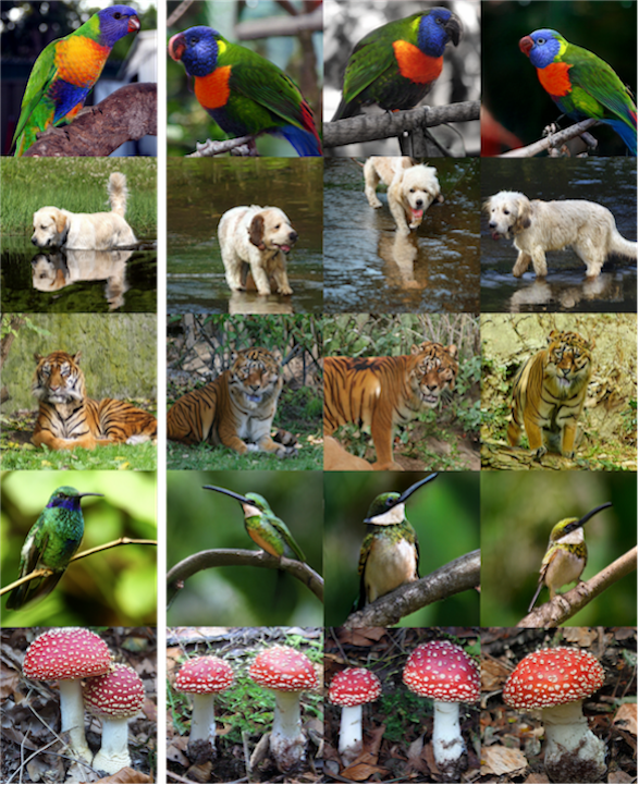
(a) IC-GAN samples

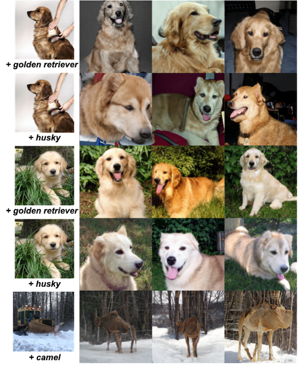
(b) Class-conditional IC-GAN samples

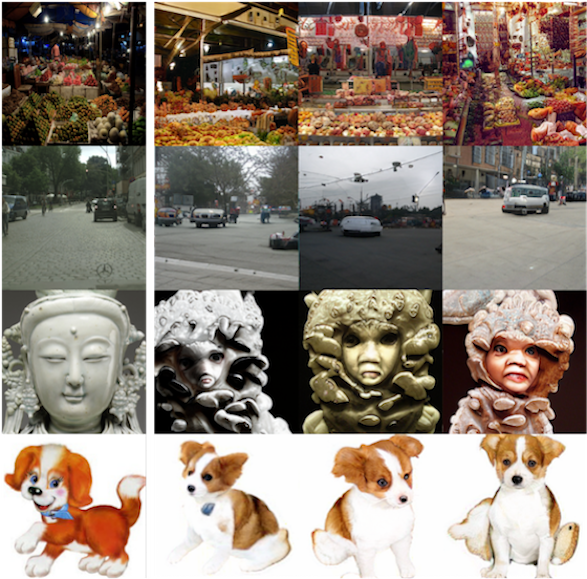
(c) IC-GAN transfer samples

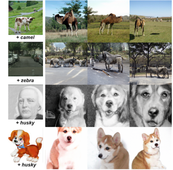
(d) Class-conditional IC-GAN transfer samples

Figure 1: Samples from unlabeled (a) and class-conditional (b) IC-GAN trained on the $256\!\times\!256$ ImageNet dataset. For each subfigure, the first column represents instances used to condition the model and the next three columns depict model samples. For class-conditional generation in (b) we include samples conditioned on the same image but different labels. We highlight the generalization capacities of IC-GAN by applying the ImageNet-trained model to instances from other datasets in unlabeled (c) and class-conditional (d) scenarios. Panels (c) and (d) display samples conditioned on instances from the COCO-Stuff, Cityscapes, MetFaces, and PACS datasets (from top to bottom).

In this work, we introduce a new approach, called instance-conditioned GAN (IC-GAN), which extends the GAN framework to model a mixture of local data densities. More precisely, IC-GAN learns to model the distribution of the neighborhood of a data point, also referred to as instance, by providing a representation of the instance as an additional input to both the generator and discriminator, and by using the neighbors of the instance as real samples for the discriminator. By choosing a sufficiently large neighborhood around the conditioning instance, we avoid the pitfall of excessively partitioning the data into small clusters. Given the overlapping nature of these clusters, increasing the number of partitions does not come at the expense of having less samples in each of them. Moreover, unlike when conditioning on discrete cluster indices, conditioning on instance representations naturally leads the generator to produce similar samples for similar instances. Interestingly, once trained, our IC-GAN can be used to effortlessly transfer to other datasets not seen during training by simply swapping-out the conditioning instances at inference time.

IC-GAN bears similarities with kernel density estimation (KDE), a non-parametric density estimator in the form of a mixture of parametrized kernels modeling the density around each training data point – see e.g. [4]. Similar to KDE, IC-GAN can be seen as a mixture density estimator, where each component is obtained by conditioning on a training instance. Unlike KDE, however, we do not model the data likelihood explicitly, but take an adversarial approach in which we model the local density implicitly with a neural network that takes as input the conditioning instance as well as a noise vector. Therefore, the kernel in IC-GAN is no longer independent on the data point on which we condition, and instead of a kernel bandwidth parameter, we control the smoothness by choosing the neighborhood size of an instance from which we sample the real samples to be fed to the discriminator.

We validate our approach on two image generation tasks: (1) unlabeled image generation where there is no class information available, and (2) class-conditional image generation. For the unlabeled scenario, we report results on the ImageNet and COCO-Stuff datasets. We show that IC-GAN outperforms previous approaches in unlabeled image generation on both datasets. Additionally, we perform a series of transfer experiments and demonstrate that an IC-GAN trained on ImageNet achieves better generation quality and diversity when testing on COCO-Stuff than the same model trained on COCO-Stuff. In the class-conditional setting, we show that IC-GAN can generate images with controllable semantics – by adapting both class and instance–, while achieving competitive sample quality and diversity on the ImageNet dataset. Finally, we test IC-GAN in ImageNet-LT, a long-tail class distribution ablated version of ImageNet, highlighting the benefits of non-parametric density estimation in datasets with unbalanced classes. Figure 1 shows IC-GAN unlabeled ImageNet generations (a), IC-GAN class-conditional ImageNet generations (b), and IC-GAN transfer generations both in the unlabeled (c) and controllable class-conditional (d) setting.

2 Instance-conditioned GAN

The key idea of IC-GAN is to model the distribution of a complex dataset by leveraging fine-grained overlapping clusters in the data manifold, where each cluster is described by a datapoint $\mathbf{x}_{i}$ – referred to as instance – and its nearest neighbors set $\mathcal{A}_{i}$ in a feature space. Our objective is to model the underlying data distribution $p(\mathbf{x})$ as a mixture of conditional distributions $p(\mathbf{x}|\mathbf{h}_{i})$ around each of $M$ instance feature vectors $\mathbf{h}_{i}$ in the dataset, such that $p(\mathbf{x})\approx\frac{1}{M}\sum_{i}p(\mathbf{x}|\mathbf{h}_{i})$.

More precisely, given an unlabeled dataset $\mathcal{D}=\{\mathbf{x}_{i}\}_{i=1}^{M}$ with $M$ data samples $\mathbf{x}_{i}$ and an embedding function $f$ parametrized by $\phi$, we start by extracting instance features $\mathbf{h}_{i}=f_{\phi}(\mathbf{x}_{i})\;\forall\mathbf{x}_{i}\in\mathcal{D}$, where $f_{\phi}(\cdot)$ is learned in an unsupervised or self-supervised manner. We then define the set $\mathcal{A}_{i}$ of $k$ nearest neighbors for each data sample using the cosine similarity – as is common in nearest neighbor classifiers, e.g. [53, 54] – over the features $\mathbf{h}_{i}$. Figure 2(a) depicts a sample $\mathbf{x}_{i}$ and its nearest neighbors.

We are interested in implicitly modelling the conditional distributions $p(\mathbf{x}|\mathbf{h}_{i})$ with a generator $G_{\theta_{G}}(\mathbf{z},\mathbf{h}_{i})$, implemented by a deep neural network with parameters $\theta_{G}$. The generator transforms samples from a unit Gaussian prior $\mathbf{z}\sim\mathcal{N}(0,I)$ into samples $\mathbf{x}$ from the conditional distribution $p(\mathbf{x}|\mathbf{h}_{i})$, where $\mathbf{h}_{i}$ is the feature vector of an instance $\mathbf{x}_{i}$ sampled from the training data. In IC-GAN, we adopt an adversarial approach to train the generator $G_{\theta_{G}}$. Therefore, our generator is jointly trained with a discriminator $D_{\theta_{D}}(\mathbf{x},\mathbf{h}_{i})$ that discerns between real neighbors and generated neighbors of $\mathbf{h}_{i}$, as shown in Figure 2(b). Note that for each $\mathbf{h}_{i}$, real neighbors are sampled uniformly from $\mathcal{A}_{i}$.

Both $G$ and $D$ engage in a two player min-max game where they try to find the Nash equilibrium for the following equation:

$$\begin{split}\min_{G}\max_{D}\;&\mathbb{E}_{\mathbf{x}_{i}\sim p(\mathbf{x}),\mathbf{x}_{n}\sim\mathcal{U}(\mathcal{A}_{i})}[\log D(\mathbf{x}_{n},f_{\phi}(\mathbf{x}_{i}))]\;+\\ &\hskip 5.0pt\mathbb{E}_{\mathbf{x}_{i}\sim p(\mathbf{x}),\mathbf{z}\sim p(\mathbf{z})}[\log(1-D(G(\mathbf{z},f_{\phi}(\mathbf{x}_{i})),f_{\phi}(\mathbf{x}_{i})))].\end{split}$$ (1)

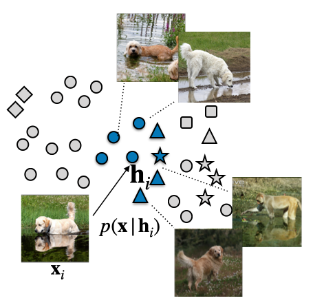
(a) Neighborhood $\mathcal{A}_{i}$ of instance $\mathbf{h}_{i}$

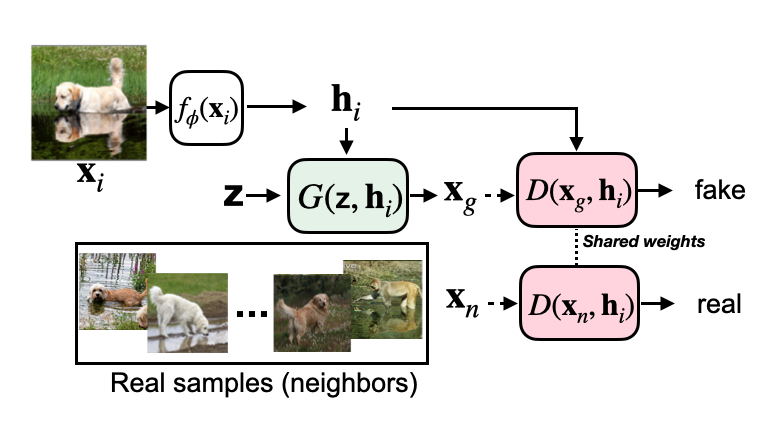
(b) Schematic illustration of the IC-GAN workflow

Figure 2: Overview of IC-GAN. (a) The goal of the generator is to generate realistic images similar to the neighbors of $\mathbf{h}_{i}$, defined in the embedding space using cosine similarity. Five out of seven neighbors are shown in the figure. Note that images in the same neighborhood may belong to different classes (depicted as different shapes). (b) Conditioned on instance features $\mathbf{h}_{i}$ and noise $\mathbf{z}$, the generator produces a synthetic sample $\mathbf{x}_{g}$. Generated samples and real samples (neighbors of $\mathbf{h}_{i}$) are fed to the discriminator, which is conditioned on the same $\mathbf{h}_{i}$.

Note that when training IC-GAN we use all available training datapoints to condition the model. At inference time, as in non-parametric density estimation methods such as KDE, the generator of IC-GAN also requires instance features, which may come from the training distribution or a different one.

Extension to class-conditional generation. We extend IC-GAN for class-conditional generation by additionally conditioning the generator and discriminator on a class label $\mathbf{y}$. More precisely, given a labeled dataset $\mathcal{D}_{l}=\{(\mathbf{x}_{i},\mathbf{y}_{i})\}_{i=1}^{M}$ with $M$ data sample pairs $(\mathbf{x}_{i},\mathbf{y}_{i})$ and an embedding function $f_{\phi}$, we extract instance features $\mathbf{h}_{i}=f_{\phi}(\mathbf{x}_{i})\;\forall\mathbf{x}_{i}\in\mathcal{D}_{l}$, where $f_{\phi}(\cdot)$ is learned in an unsupervised, self-supervised, or supervised manner. We then define the set $\mathcal{A}_{i}$ of $k$ nearest neighbors for each data sample using the cosine similarity over the features $\mathbf{h}_{i}$, where neighbors may be from different classes. This results in neighborhoods, where the number of neighbors belonging to the same class as the instance $\mathbf{h}_{i}$ is often smaller than $k$. During training, real neighbors $\mathbf{x}_{j}$ and their respective labels $\mathbf{y}_{j}$ are sampled uniformly from $\mathcal{A}_{i}$ for each $\mathbf{h}_{i}$. In the class-conditional case, we model $p(\mathbf{x}|\mathbf{h}_{i},\mathbf{y}_{j})$ with a generator $G_{\theta_{G}}(\mathbf{z},\mathbf{h}_{i},\mathbf{y}_{j})$ trained jointly with a discriminator $D_{\theta_{D}}(\mathbf{x},\mathbf{h}_{i},\mathbf{y}_{j})$.

3 Experimental evaluation

We describe our experimental setup in Section 3.1, followed by results presented in the unlabeled setting in Section 3.2, dataset transfer in Section 3.3 and class-conditional generation in Section 3.4. We analyze the impact of the number of stored instances and neighborhood size in Section 3.5.

3.1 Experimental setup

Datasets. We evaluate our model in the unlabeled scenario on ImageNet [45] and COCO-Stuff [6]. The ImageNet dataset contains 1.2M and 50k images for training and evaluation, respectively. COCO-Stuff is a very diverse and complex dataset which contains multi-object images and has been widely used for complex scene generation. We use the train and evaluation splits of [8], and the (un)seen subsets of the evaluation images with only class combinations that have (not) been seen during training. These splits contain 76k, 2k, 675 and 1.3k images, respectively. For the class-conditional image generation, we use ImageNet as well as ImageNet-LT [34]. The latter is a long-tail variant of ImageNet that contains a subset of 115k samples, where the 1,000 classes have between 5 and 1,280 samples each. Moreover, we use some samples of four additional datasets to highlight the transfer abilities of IC-GAN: Cityscapes [10], MetFaces [28], PACS [31] and Sketches [15].

Evaluation protocol. We report Fréchet Inception Distance (FID) [22], Inception Score (IS) [47], and LPIPS [57]. LPIPS computes the distance between the AlexNet activations of two images generated with two different latent vectors and same conditioning. On ImageNet, we follow [5], and compute FID over 50k generated images and the 50k real validation samples are used as reference. On COCO-Stuff and ImageNet-LT, we compute the FID for each of the splits using all images in the split as reference, and sample the same number images. Additionally, in ImageNet-LT we stratify the FID by grouping classes based on the number of train samples: more than 100 (many-shot FID), between 20 and 100 (med-shot FID), and less than 20 (few-shot FID). For the reference set, we split the validation images along these three groups of classes, and generate a matching number of samples per group. In order to compute all above-mentioned metrics, IC-GAN requires instance features for sampling. Unless stated otherwise, we store 1,000 training set instances by applying k-means clustering to the training set and selecting the features of the data point that is the closest to each one of the centroids. All quantitative metrics for IC-GAN are reported over five random seeds for the input noise when sampling from the model.

Network architectures and hyperparameters. As feature extractor $f_{\phi}$, we use a ResNet50 [21] trained in a self-supervised way with SwAV [7] for the unlabeled scenario; for the class-conditional IC-GAN, we use a ResNet50 trained for the classification task on either ImageNet or ImageNet-LT [26]. For ImageNet experiments, we use BigGAN [5] as a baseline architecture, given its superior image quality and ubiquitous use in conditional image generation. For IC-GAN, we replace the class embedding layers in the generator by a fully connected layer that takes the instance features as input and reduces its dimensionality from 2,048 to 512; the same approach is followed to adapt the discriminator. For COCO-Stuff, we additionally include the state-of-the-art unconditional StyleGAN2 architecture [29], as it has shown good generation quality and diversity in the lower data regime [28, 29]. We follow its class-conditional version [28] to extend it to IC-GAN by replacing the input class embedding by the instance features. Unless stated otherwise, we set the size of the neighborhoods to $k\!=\!50$ for ImageNet and $k\!=\!5$ for both COCO-Stuff and ImageNet-LT. See the supplementary material for details on the architecture and optimization hyperparameters.

3.2 Unlabeled setting

Table 1: Results for ImageNet in unlabeled setting. For fair comparison with [42] at $64\!\times\!64$ resolution, we trained an unconditional BigGAN model and report the non-official FID and IS scores – computed with Pytorch rather than TensorFlow – indicated with *. ^†: increased parameters to match IC-GAN capacity. DA: 50% horizontal flips in (d) real and fake samples, and (i) conditioning instances. $ch\times$: Channel multiplier that affects network width as in BigGAN.

Method	Res.	$\downarrow$FID	$\uparrow$IS
Self-sup. GAN  [42]	64	19.2*	16.5*
Uncond. BigGAN†	64	16.9* $\pm$ 0.0	14.6* $\pm$ 0.1
IC-GAN	64	10.4* $\pm$ 0.1	21.9* $\pm$ 0.1
IC-GAN + DA (d,i)	64	9.2* $\pm$ 0.0	23.5* $\pm$ 0.1
MGAN [23]	128	58.9	13.2
PacGAN2 [32]	128	57.5	13.5
Logo-GAN-AE [46]	128	50.9	14.4
Self-cond. GAN [33]	128	41.7	14.9
Uncond. BigGAN [36]	128	25.3	20.4
SS-cluster GAN [36]	128	22.0	23.5
PGMGAN [2]	128	21.7	23.3
IC-GAN	128	13.2 $\pm$ 0.0	45.5 $\pm$ 0.2
IC-GAN + DA (d,i)	128	11.7 $\pm$ 0.0	48.7 $\pm$ 0.1
ADM [12]	256	32.5	37.6
IC-GAN ($ch\times 64$)	256	17.0 $\pm$ 0.2	53.0 $\pm$ 0.4
IC-GAN ($ch\times 64$) + DA (d,i)	256	17.4 $\pm$ 0.1	53.5 $\pm$ 0.5
IC-GAN ($ch\times 96$) + DA (d)	256	15.6 $\pm$ 0.1	59.0 $\pm$ 0.4

ImageNet. We start by comparing IC-GAN against previous work in Table 1. Note that unconditional BigGAN baseline is trained by setting all labels in the training set to zero, following [36, 42]. IC-GAN surpasses all previous approaches at both $64\!\times\!64$ and $128\!\times\!128$ resolutions in both FID and IS scores. At $256\!\times\!256$ resolution, IC-GAN outperforms the concurrent unconditional diffusion-based model of [12]; the only other result we are aware of in this setting. Additional results in terms of precision and recall can be found in Table 8 in the supplementary material.

As shown in Figure 1(a), IC-GAN generates high quality images preserving most of the appearance of the conditioning instance. Note that generated images are not mere training memorizations; as shown in the supplementary material, generated images differ substantially from the nearest training samples.

COCO-Stuff. We proceed with the evaluation of IC-GAN on COCO-Stuff in Table 2. We also compare to state-of-the-art complex scene generation pipelines which rely on labeled bounding box annotations as conditioning – LostGANv2 [49] and OC-GAN [50]. Both of these approaches use tailored architectures for complex scene generation, which have at least twice the number of parameters of IC-GAN. Our IC-GAN matches or improves upon the unconditional version of the same backbone architecture in terms of FID in all cases, except for training FID with the StyleGAN2 backbone at $256\!\times\!256$ resolution. Overall, the StyleGAN2 backbone is superior to BigGAN on this dataset, and StyleGAN2-based IC-GAN achieves the state-of-the-art FID scores, even when compared to the bounding-box conditioned LostGANv2 and OC-GAN. IC-GAN exhibits notably higher LPIPS than LostGANv2 and OC-GAN, which could be explained by the fact that the latter only leverage one real sample per input conditioning during training; whereas IC-GAN uses multiple real neighboring samples per each instance, naturally favouring diversity in the generated images. As shown in figures 3(b) and 3(c), IC-GAN generates high quality diverse images given the input instance. A qualitative comparison between LostGANv2, OC-GAN and IC-GAN can be found in Section E of the supplementary material.

Table 2: Quantitative results on COCO-Stuff. IC-GAN trained on ImageNet indicated as “transf”. Some non-zero standard deviations are reported as 0.0 because of rounding.

		$\downarrow$FID				$\uparrow$ LPIPS
128$\times$128	# prms.	train	eval	eval seen	eval unseen	eval
LostGANv2 [49]	41 M	12.8 $\pm$ 0.1	40.7 $\pm$ 0.3	80.0 $\pm$ 0.4	55.2 $\pm$ 0.5	0.45 $\pm$ 0.1
OC-GAN [50]	170 M	—	45.1 $\pm$ 0.3	85.8 $\pm$ 0.5	60.1 $\pm$ 0.2	0.13 $\pm$ 0.1
Unconditional (BigGAN)	18 M	17.9 $\pm$ 0.1	46.9 $\pm$ 0.5	103.8 $\pm$ 0.8	60.9 $\pm$ 0.7	0.68 $\pm$ 0.1
IC-GAN (BigGAN)	22 M	16.8 $\pm$ 0.1	44.9 $\pm$ 0.5	81.5 $\pm$ 1.3	60.5 $\pm$ 0.5	0.67 $\pm$ 0.1
IC-GAN (BigGAN, transf.)	77 M	8.5 $\pm$ 0.0	35.6 $\pm$ 0.2	77.0 $\pm$ 1.0	48.9 $\pm$ 0.2	0.69 $\pm$ 0.1
Unconditional (StyleGAN2)	23 M	8.8 $\pm$ 0.1	37.8 $\pm$ 0.2	92.1 $\pm$ 1.0	53.2 $\pm$ 0.5	0.68 $\pm$ 0.1
IC-GAN (StyleGAN2)	24 M	8.9 $\pm$ 0.0	36.2 $\pm$ 0.2	74.3 $\pm$ 0.8	50.8 $\pm$ 0.3	0.67 $\pm$ 0.1
256$\times$256
LostGANv2 [49]	46 M	18.0 $\pm$ 0.1	47.6 $\pm$ 0.4	88.5 $\pm$ 0.4	62.0 $\pm$ 0.6	0.56 $\pm$ 0.1
OC-GAN [50]	190 M	—	57.0 $\pm$ 0.1	98.7 $\pm$ 1.2	71.4 $\pm$ 0.5	0.21 $\pm$ 0.1
Unconditional (BigGAN)	21 M	51.0 $\pm$ 0.1	81.6 $\pm$ 0.5	135.1 $\pm$ 1.6	95.8 $\pm$ 1.1	0.77 $\pm$ 0.1
IC-GAN (BigGAN)	26 M	24.6 $\pm$ 0.1	53.1 $\pm$ 0.4	88.5 $\pm$ 1.8	69.1 $\pm$ 0.6	0.73 $\pm$ 0.1
IC-GAN (BigGAN, transf.)	90 M	13.9 $\pm$ 0.1	40.9 $\pm$ 0.3	79.4 $\pm$ 1.2	55.6 $\pm$ 0.6	0.76 $\pm$ 0.1
Unconditional (StyleGAN2)	23 M	7.1 $\pm$ 0.0	44.6 $\pm$ 0.4	98.1 $\pm$ 1.7	59.9 $\pm$ 0.5	0.76 $\pm$ 0.1
IC-GAN (StyleGAN2)	25 M	9.6 $\pm$ 0.0	41.4 $\pm$ 0.2	76.7 $\pm$ 0.6	57.5 $\pm$ 0.5	0.74 $\pm$ 0.1

(a) $\mathbf{x}_{i}$

(b) IC-GAN (StyleGAN2)

(c) IC-GAN (BigGAN)

(d) IC-GAN (BigGAN, transf.)

Figure 3: Qualitative comparison for scene generation on $256\!\times\!256$ COCO-Stuff.

3.3 Off-the-shelf transfer to other datasets

In our first transfer experiment, we train IC-GAN with a BigGAN architecture on ImageNet, and use it to generate images from COCO-Stuff instances at test time. Quantitative results are reported as “IC-GAN (transf.)” in Table 2. In this setup, no COCO-Stuff images are used to train the model, thus, all splits contain unseen objects combinations. Perhaps surprisingly, IC-GAN trained on ImageNet outperforms the same model trained on COCO-Stuff for all splits: 8.5 vs. 16.8 train FID at 128 resolution. This raises the question of how close ImageNet and COCO-Stuff data distributions are. We compute the FID between real data train split of the two datasets at $128\!\times\!128$ resolution and obtain a score of $37.2$. Hence, the remarkable transfer capabilities of IC-GAN are not explained by dataset similarity and may be attributed to the effectiveness of the ImageNet pre-trained feature extractor and generator. When we replace the conditioning instances from COCO-Stuff with those of ImageNet, we obtain a train FID score of 43.5, underlining the important distribution shift that can be implemented by changing the conditioning instances.

Interestingly, the transferred IC-GAN also outperforms LostGANv2 and OC-GAN which condition on labeled bounding box annotations. Transferring the model from ImageNet boosts diversity w.r.t. the model trained on COCO-Stuff (see LPIPS in Table 2), which may be in part due to the larger $k\!=\!50$ used for ImageNet training, compared to $k\!=\!5$ when training on COCO-Stuff. Qualitative results of COCO-Stuff generations from the ImageNet pre-trained IC-GAN can be found in Figure 1(c) (top row) and Figure 3(d). These generations suggest that IC-GAN is able to effectively leverage the large scale training on ImageNet to improve the quality and diversity of the COCO-Stuff scene generation, which contains significantly less data to train.

We further explore how the ImageNet trained IC-GAN transfers to conditioning on other datasets using Cityscapes, MetFaces, and PACS in Figure 1(c). Generated images still preserve the semantics and style of the images for all datasets, although degrading their quality when compared to samples in Figure 1(a), as the instances in these datasets –in particular MetFaces and PACS– are very different from the ImageNet ones. See Section F in the supplementary material for more discussion, additional evaluations, and more qualitative examples of dataset transfer.

3.4 Class-conditional setting

Table 3: Class-conditional results on ImageNet. *: Trained using open source code. DA: 50% horizontal flips in (d) real and fake samples, and (i) conditioning instances. $ch\times$: Channel multiplier that affects network width. ^†: numbers from the original paper, as training diverged with the BigGAN opensourced code.

	Res.	$\downarrow$FID	$\uparrow$IS
BigGAN* [5]	64	12.3 $\pm$ 0.0	27.0 $\pm$ 0.2
BigGAN* [5] + DA (d)	64	10.2 $\pm$ 0.1	30.1 $\pm$ 0.1
IC-GAN	64	8.5 $\pm$ 0.0	39.7 $\pm$ 0.2
IC-GAN + DA(d, i)	64	6.7 $\pm$ 0.0	45.9 $\pm$ 0.3
BigGAN* [5]	128	9.4 $\pm$ 0.0	98.7 $\pm$ 1.1
BigGAN* [5] + DA(d)	128	8.0 $\pm$ 0.0	107.2 $\pm$ 0.9
IC-GAN	128	10.6 $\pm$ 0.1	100.1 $\pm$ 0.5
IC-GAN + DA(d, i)	128	9.5 $\pm$ 0.1	108.6 $\pm$ 0.7
BigGAN* [5] ($ch\times 64$)	256	8.0 $\pm$ 0.1	139.1 $\pm$ 0.3
BigGAN* [5] ($ch\times 64$) + DA(d)	256	8.3 $\pm$ 0.1	125.0 $\pm$ 1.1
IC-GAN ($ch\times 64$)	256	8.3 $\pm$ 0.1	143.7 $\pm$ 1.1
IC-GAN ($ch\times 64$) + DA(d, i)	256	7.5 $\pm$ 0.0	152.6 $\pm$ 1.1
BigGAN† [5] ($ch\times 96$)	256	8.1	144.2
IC-GAN ($ch\times 96$) + DA(d)	256	8.2 $\pm$ 0.1	173.8 $\pm$ 0.9

ImageNet. In Table 3, we show that the class-conditioned IC-GAN outperforms BigGAN in terms of both FID and IS across all resolutions except the FID at $128\!\times\!128$ resolution. It is worth mentioning that, unlike BigGAN, IC-GAN can control the semantics of the generated images by either fixing the instance features and swapping the class conditioning, or by fixing the class conditioning and swapping the instance features; see Figure 1(b). As shown in the figure, generated images preserve semantics of both the class label and the instance, generating different dog breeds on similar backgrounds, or generating camels in the snow, an unseen scenario in ImageNet to the best of our knowledge. Moreover, in Figure 1(d), we show the transfer capabilities of our class-conditional IC-GAN trained on ImageNet and conditioned on instances from other datasets, generating camels in the grass, zebras in the city, and husky dogs with the style of MetFaces and PACS instances. These controllable conditionings enable the generation of images that are not present or very rare in the ImageNet dataset, e.g. camels surrounded by snow or zebras in the city. Additional qualitative transfer results which either fix the class label and swap the instance features, or vice-versa, can be found in Section F of the supplementary material.

ImageNet-LT. Due to the class imbalance in ImageNet-LT, selecting a subset of instances with either k-means or uniform sampling can easily result in ignoring rare classes, and penalizing their generation. Therefore, for this dataset we use all available 115k training instances to sample from the model and compute the metrics. In Table 4 we compare to BigGAN, showing that IC-GAN is better in terms of FID and IS for modeling this long-tailed distribution. Note that the improvement is noticeable for each of the three groups of classes with different number of samples, see many/med/few column. In Section G of the supplementary material we present experiments when using class-balancing to train BigGAN, showing that it does not improve quality nor diversity of generated samples. We hypothesize that oversampling some classes may result in overfitting for the discriminator, leading to low quality image generations.

3.5 Selection of stored instances and neighborhood size

In this section, we empirically justify the k-means procedure to select the instances to sample from the model, consider the effect of the number of instances used to sample from the model, as well as the effect of the size $k$ of the neighborhoods $\mathcal{A}_{i}$ used during training. The impact of different choices for the instance embedding function $f_{\phi}(\mathbf{x})$ is evaluated in the supplementary material.

Table 4: Class-conditional results on ImageNet-LT. *: Trained using open source code.

	Res.	$\downarrow$train FID	$\uparrow$train IS	$\downarrow$val FID	many/med/few $\downarrow$val FID	$\uparrow$val IS
BigGAN* [5]	64	27.6 $\pm$ 0.1	18.1 $\pm$ 0.2	28.1 $\pm$ 0.1	28.8 / 32.8 / 48.4 $\pm$ 0.2	16.0 $\pm$ 0.1
IC-GAN	64	23.2 $\pm$ 0.1	19.5 $\pm$ 0.1	23.4 $\pm$ 0.1	23.8 / 28.0 / 42.7 $\pm$ 0.1	17.6 $\pm$ 0.1
BigGAN* [5]	128	31.4 $\pm$ 0.1	30.6 $\pm$ 0.1	35.4 $\pm$ 0.1	34.0 / 43.5 / 64.4 $\pm$ 0.2	24.9 $\pm$ 0.2
IC-GAN	128	23.4 $\pm$ 0.1	39.6 $\pm$ 0.2	24.9 $\pm$ 0.1	24.3 / 31.4 / 53.6 $\pm$ 0.3	32.5 $\pm$ 0.1
BigGAN* [5]	256	27.8 $\pm$ 0.0	58.2 $\pm$ 0.2	31.4 $\pm$ 0.1	28.1 / 40.9 / 67.6 $\pm$ 0.3	44.7 $\pm$ 0.2
IC-GAN	256	21.7 $\pm$ 0.1	66.5 $\pm$ 0.3	23.4 $\pm$ 0.1	20.6 / 32.4 / 60.0 $\pm$ 0.2	51.7 $\pm$ 0.1

Selecting instances to sample from the model. In Figure 4 (left), we compare two instance selection methods in terms of FID: uniform sampling (Random) and k-means (Clustered), where we select the closest instance to each cluster centroid, using $k\!=\!50$ neighbors during training (solid and dotted green lines). Random selection is consistently outperformed by k-means; selecting only 1,000 instances with k-means results in better FID than randomly selecting 5,000 instances. Moreover, storing more than 1,000 instances selected with k-means does not result in noticeable improvements in FID. Additionally, we computed FID metrics for the 1,000 ground truth images that are closest to the k-means cluster centers, obtaining $41.8\pm 0.2$ FID, which is considerably higher than the $10.4\pm 0.1$ FID we obtain with IC-GAN ($k=50$) when using the same 1,000 cluster centers. This supports the idea that IC-GAN is generating data points that go beyond the stored instances, better recovering the data distribution.

We consider precision (P) and recall (R) [30] (using an InceptionV3 [51] as feature extractor and sampling 10,000 generated and real images) to disentangle the factors driving the improvement in FID, namely image quality and diversity (coverage) – see Figure 4 (right). We see that augmenting the number of stored instances results in slightly worse precision (image quality) but notably better recall (coverage). Intuitively, this suggests that by increasing the number of stored instances, we can better recover the data density at the expense of slightly degraded image quality in lower density regions of the manifold – see e.g. [11].

Figure 4: Impact on the number of stored instances used to evaluate IC-GAN and the size of the neighborhood $k$. Experiments performed on the $64\!\times\!64$ unlabeled ImageNet dataset.

Neighborhood size. In Figure 4 (both panels) we analyze the interplay between the neighborhood size and the number of instances used to recover the data distribution. For small numbers of stored instances, we observe that larger the neighborhoods lead to better (lower) FID scores (left-hand side of left panel). For recall, we also observe improvements for large neighborhoods when storing few instances (left-hand side of right panel), suggesting that larger neighborhoods are more effective in recovering the data distribution from few instances. This trend is reverted for large numbers of stored instances, where smaller values of k are more effective. This supports the idea that the neighborhood size acts as a bandwidth parameter – similar to KDE –, that controls the smoothness of the implicitly learnt conditional distributions around instances. For example, $k=500$ leads to smoother conditional distributions than $k=5$, and as a result requires fewer stored instances to recover the data distribution. Moreover, as expected, we notice that the value of $k$ does not significantly affect precision (right panel). Overall, $k=50$ offers a good compromise, exhibiting top performance across all metrics when using at least $500$ stored instances. We visualize the smoothness effect by means of a qualitative comparison across samples from different neighborhood sizes in Section K of the supplementary material. Using (very) small neighborhoods (e.g. of $k=5$), results in lower diversity in the generated images.

4 Related work

Data partitioning for GANs. Previous works have attempted to improve the image generation quality and diversity of GANs by partitioning the data manifold through clustering techniques [2, 19, 33, 36, 42, 46], or by leveraging mixture models in their design [14, 17, 23]. In particular, [36, 46] apply k-means on representations from a pre-trained feature extractor to cluster the data, and then use cluster indices to condition the generator network. Then, [19, 33] introduce an alternating two-stage approach where the first stage applies k-means to the discriminator feature space and the second stage trains a GAN conditioned on the cluster indices. Similarly, [42] proposes to train a clustering network, which outputs pseudolabels, in cooperation with the generator. Further, [2] trains a feature extractor with self-supervised pre-training tasks, and creates a k-nearest neighbor graph in the learned representation space to cluster connected points into the same sub-manifold. In this case, a different generator is then trained for each identified sub-manifold. By contrast, IC-GAN uses fine-grained overlapping data neighborhoods in tandem with conditioning on rich feature embeddings (instances) to learn a localized distribution around each data point.

Mitigating mode collapse in GANs. Works which attempt to mitigate mode collapse may also bear some similarities to ours. In [32], the discriminator takes into consideration multiple random samples from the same class to output a decision. In [35], a mixed batch of generated and real samples is fed to the discriminator with the goal of predicting the ratio of real samples in the batch. Other works use a mixture of generators [17, 23] and encourage each generator to focus on generating samples from a different mode. Similarly, in [14], the discriminator is pushed to form clusters in its representation space, where each cluster is represented by a Gaussian kernel. In turn, the generator tends to learn to generate samples covering all clusters, hence mitigating mode collapse. By contrast, we focus on discriminating between real and generated neighbors of an instance conditioning, by using a single generator network trained following the GAN formulation.

Conditioning on feature vectors. Very recent work [37] uses image self-supervised feature representations to condition a generative model whose objective is to produce a good input reconstruction; this requires storing the features of all training samples. In contrast, our objective is to learn a localized distribution (as captured by nearest neighboring images) around each conditioning instance, and we only need to save a very small subset of the dataset features to approximately recover the training distribution.

Kernel density estimation and adversarial training. Connections between adversarial training and nonparametric density estimation have been made in prior work [1]. However, to the best of our knowledge, no prior work models the dataset density in a nonparametric fashion with a localized distribution around each data point with a single conditional generation network.

Complex scene generation. Existing methods for complex scene generation, where natural looking scenes contain multiple objects, most often aim at controllability and rely on detailed conditionings such as a scene graphs [3, 25], bounding box layouts [48, 49, 50, 58], semantic segmentation masks [9, 43, 44, 52, 55] or more recently, freehand sketches [16]. All these methods leverage intricate pipelines to generate complex scenes and require labeled datasets. By contrast, our approach relies on instance conditionings which control the global semantics of the generation process, and does not require any dataset labels. It is worth noting that complex scene generation is often characterized by unbalanced, strongly long tailed datasets. Long-tail class distributions negatively affect class-conditional GANs, as they struggle to generate visually appealing samples for classes in the tail [8]. However, to the best of our knowledge, no other previous work tackles this problem for GANs.

5 Discussion

Contributions. We presented instance-conditioned GAN (IC-GAN), which models dataset distributions in a non-parametric way by conditioning both generator and discriminator on instance features. We validated our approach on the unlabeled setting, showing consistent improvements over baselines on ImageNet and COCO-Stuff. Moreover, we showed through transfer experiments, where we condition the ImageNet-trained model on instances of other datasets, the ability of IC-GAN to produce compelling samples from different data distributions. Finally, we validated IC-GAN in the class-conditional setting, obtaining competitive results on ImageNet and surpassing the BigGAN baseline on the challenging ImageNet-LT; and showed compelling controllable generations by swapping the class-conditioning given a fixed instance or the instance given a fixed conditioning.

Limitations. IC-GAN showed excellent image quality for labeled (class-conditional) and unlabeled image generation. However, as any machine learning tool, it has some limitations. First, as kernel density estimator approaches, IC-GAN requires storing training instances to use the model. Experimentally, we noticed that for complex datasets, such as ImageNet, using 1,000 instances is enough to approximately cover the dataset distribution. Second, the instance feature vectors used to condition the model are obtained with a pre-trained feature extractor (self-supervised in the unlabeled case) and depend on it. We speculate that this limitation might be mitigated if the feature extractor and the generator are trained jointly, and leave it as future work. Third, although, we highlighted excellent transfer potential of our approach to unseen datasets, we observed that, in the case of transfer to datasets that are very different from ImageNet, the quality of generated images degrades.

Broader impacts. IC-GAN brings with it several benefits such as excellent image quality in labeled (class-conditional) and unlabeled image generation tasks, and the transfer potential to unseen datasets, enabling the use of our model on a variety of datasets without the need of fine-tuning or re-training. Moreover, in the case of class-conditional image generation, IC-GAN enables controllable generation of content by adapting either the style – by changing the instance – or the semantics – by altering the class –. Thus, we expect that our model can positively affect the workflow for creative content generators. That being said, with improving image quality in generative modeling, there is some potential for misuse. A common example are deepfakes, where a generative model is used to manipulate images or videos well enough that humans cannot distinguish real from fake, with the intent to misinform. We believe, however, that open research on generative image models also contributes to better understand such synthetic content, and to detect it where it is undesirable. Recently, the community has also started to undertake explicit efforts towards detecting manipulated content by organizing challenges such as the Deepfake Detection Challenge [13].

Instance-Conditioned GAN: Supplementary Material

We provide additional material to support the main paper. We credit the used assets by citing their web links and licenses in Section A, and continue by describing the experimental setup and used hyperparameters in Section B. We compute Precision and Recall metrics on ImageNet in Section C, and we further compare BigGAN and StyleGAN2 backbones for IC-GAN on ImageNet in Section D. We provide additional qualitative results for both IC-GAN on ImageNet in Section E and IC-GAN off-the-shelf transfer results on other datasets in Section F. Moreover, we provide results when training BigGAN with class balancing on ImageNet-LT in Section G. Finally, we show further impact studies such as the choice of feature extractor (Section H), the number of conditionings used during training (Section I), matching storage requirements for unconditional counterparts of BigGAN and StyleGAN2 and IC-GAN (Section J) and the qualitative impact of neighborhood size $k$ for ImageNet, as well as quantitative results for ImageNet-LT and COCO-Stuff (Section K).

Appendix A Assets and licensing information

In Tables 5 and 6, we provide the links to the used datasets, repositories and their licenses. We use Faiss [24] for a fast computation of nearest neighbors and k-means algorithm leveraging GPUs, DiffAugment [59] for additional data augmentation when training BigGAN, and the pre-trained SwAV [7] and ResNet50 models on ImageNet-LT [26] to extract instance features.

Table 5: Links to the assets used in the paper.

Name	GitHub link
ImageNet [45]	https://www.image-net.org
ImageNet-LT [34]	https://github.com/zhmiao/OpenLongTailRecognition-OLTR
COCO-Stuff [6]	https://cocodataset.org/
Cityscapes [10]	https://www.cityscapes-dataset.com/
MetFaces [28]	https://github.com/NVlabs/metfaces-dataset
PACS [31]	https://domaingeneralization.github.io/
Sketches [15]	http://cybertron.cg.tu-berlin.de/eitz/projects/classifysketch/
BigGAN [5]	https://github.com/ajbrock/BigGAN-PyTorch
StyleGAN2 [28]	https://github.com/NVlabs/stylegan2-ada-pytorch
Faiss [24]	https://github.com/facebookresearch/faiss
DiffAugment [59]	https://github.com/mit-han-lab/data-efficient-gans
PRDC [41]	https://github.com/clovaai/generative-evaluation-prdc
SwAV [7]	https://github.com/facebookresearch/swav
Pre-trained ResNet50 [26]	https://github.com/facebookresearch/classifier-balancing

Table 6: Assets licensing information.

Name	License
ImageNet [45] and ImageNet-LT [34]	Terms of access: https://www.image-net.org/download.php
COCO-Stuff [6]	https://www.flickr.com/creativecommons
Cityscapes [10]	https://www.cityscapes-dataset.com/license
MetFaces [28]	Creative Commons BY-NC 2.0
PACS [31]	Unknown
Sketches [15]	Creative Commons Attribution 4.0 International
BigGAN [5]	MIT
StyleGAN2 [28]	NVIDIA Source Code
Faiss [24]	MIT
DiffAugment [59]	BSD 2-Clause "Simplified"
PRDC [41]	MIT
swAV [7]	Attribution-NonCommercial 4.0 International
Pre-trained ResNet50 [26]	BSD

Appendix B Experimental setup and hyperparameters

We divide the experimental section into architecture modifications in Subsection B.1 and training and hyperparameter details in Subsection B.2.

B.1 Architecture modifications for IC-GAN.

In our IC-GAN experiments, we leveraged BigGAN and StyleGAN2 backbones, and extended their architectures to handle the introduced instance conditionings.

When using BigGAN as a base architecture, IC-GAN replaces the class embedding layers in both generator and discriminator by fully connected layers. The fully connected layer in the generator has an input size of $2,\!048$ (corresponding to the feature extractor $f_{\theta}$’s dimensionality) and an output size $o_{dim}$ that can be adjusted. For all our experiments, we used $o_{dim}\,=\,512$ – selected out of $\{256,512,1,\!024,2,\!048\}$. The fully connected layer in the discriminator has a variable output size $n_{dim}$ to match the dimensionality of the intermediate unconditional discriminator feature vector – following the practice in BigGAN [5]. For the class-conditional IC-GAN, we use both the class embedding layers as well as the fully connected layers associated with the instance conditioning. In particular, we concatenate class embeddings (of dimensionality $c_{dim}\,=\,128$) and instance embeddings (with dimensionality $o_{dim}\,=\,512$). To avoid the rapid growth of parameters when using both class and instance embeddings, we use $n_{dim}/2$ as the output dimensionality for each of the embeddings in the discriminator, so that the resulting concatenation has a dimensionality of $n_{dim}$.

When using StyleGAN2 as a base architecture, we modify the class-conditional architecture of [28]. In particular, we replace the class embeddings layers with a fully connected layer of output dimensionality $512$ in the generator. The fully connected layer substituting the class embedding in the discriminator is of variable size. In this case, the instance features are concatenated with the noise vector at the input of the StyleGAN2’s mapping network, creating a style vector for the generator. However, when it comes to the discriminator, the mapping network is only fed with the extracted instance features to obtain a modulating vector that is multiplied by the internal discriminator representation at each block.

All instance feature vectors $\mathbf{h}_{i}$ are normalized with $\ell_{2}$ norm before computing the neighborhoods and when used as conditioning for the GAN.

B.2 Training details and hyperparameters

All models were trained while monitoring the training FID, and training was stopped according to either one of the following criteria: (1) early stopping when FID did not improve for $50$ epochs – or the equivalent number of iterations depending on the batch size –, or (2) when the training FID diverged. For BigGAN, we mainly explored the hyperparameter space around previously known and successful configurations [5, 42]. Concretely, we focused on finding the following best hyperparameters for each dataset and resolution: the batch size ($BS$), model capacity controlled by channel multipliers ($CH$), number of discriminator updates versus generator updates ($D_{updates}$), discriminator learning rate ($D_{lr}$) and generator learning rate ($G_{lr}$), while keeping all other parameters unchanged [5]. For StyleGAN, we also performed a hyperparameter search around previously known successful settings [28]. More precisely, we searched for the optimal $D_{lr}$ and $G_{lr}$ and R1 regularization weight $\gamma$ and used default values for the other hyperparameters.

ImageNet.

When using the BigGAN backbone, in the $64\!\times\!64$ resolution, we followed the experimental setup of [42], where: $BS\!=\!256$, $CH\!=\!64$, $D_{lr}\!=\!G_{lr}\!=\!1\mathrm{e}{-4}$ and found that, although the unconditional BigGAN baseline achieves better metrics with $D_{updates}\!=\!2$, IC-GAN and BigGAN do so with $D_{updates}\!=\!1$. Note that we explored additional configurations such as increasing $BS$ or $CH$ but did not observe any improvement upon the aforementioned setup. In both the $128\!\times\!128$ and $256\!\times\!256$ resolutions, BigGAN hyperparameters were borrowed from [5]. For IC-GAN, we explored $D_{lr},G_{lr}\in\{4\mathrm{e}{-4},2\mathrm{e}{-4},1\mathrm{e}{-4},4\mathrm{e}{-5},2\mathrm{e}{-5},1\mathrm{e}{-5}\}$ and $D_{updates}\in\{1,2\}$. For $128\!\times\!128$, we used $BS\!=\!2,\!048$, $CH\!=\!96$ (as in [5]), $D_{lr}\!=\!1\mathrm{e}{-4}$, $G_{lr}\!=\!4\mathrm{e}{-5}$ and $D_{updates}\!=\!1$. For $256\!\times\!256$, we set $BS\!=\!2,\!048$ and $CH\!=\!64$ (half capacity, therefore faster training) for both BigGAN and IC-GAN, and used $D_{lr}\!=\!G_{lr}\!=\!1\mathrm{e}{-4}$ with $D_{updates}\!=\!2$ for IC-GAN. When using the StyleGAN2 architecture both as a baseline and as a backbone, we explored $BS\in\{32,64,128,256,512,1,\!024\}$, $D_{lr},G_{lr}\in\{1\mathrm{e}{-2},7\mathrm{e}{-3},5\mathrm{e}{-3},2.5\mathrm{e}{-3},1\mathrm{e}{-4},5\mathrm{e}{-4}\}$ and $\gamma\in\{2\mathrm{e}{-1},1\mathrm{e}{-2},5\mathrm{e}{-2},1\mathrm{e}{-1},2\mathrm{e}{-1},5\mathrm{e}{-1},1,2,10\}$ and selected $BS\!=\!64$ and $D_{lr}\!=\!G_{lr}\!=\!2.5\mathrm{e}{-3}$ and $\gamma\!=\!5\mathrm{e}{-2}$ for all resolutions.

COCO-Stuff.

When using BigGAN architecture, we explored $BS\in\{128,256,512,2,\!048\}$ and $CH\in\{32,48,64\}$ and found $BS\!=\!256$ and $CH\!=\!48$ to be the best choice. We searched for $D_{lr},G_{lr}\in\{1\mathrm{e}{-3},4\mathrm{e}{-4},1\mathrm{e}{-4},4\mathrm{e}{-5},1\mathrm{e}{-5}\}$ and $D_{updates}\in\{1,2\}$. For both unconditional BigGAN and IC-GAN, we chose $D_{lr}\!=\!4\mathrm{e}{-4}$ and $G_{lr}\!=\!1\mathrm{e}{-4}$ in $128\!\times\!128$ and $D_{lr}\!=\!G_{lr}\!=\!1\mathrm{e}{-4}$ in $256\!\times\!256$. For both resolutions, unconditional BigGAN uses $D_{updates}\!=\!2$ and IC-GAN, $D_{updates}\!=\!1$. When using StyleGAN2 architecture, we tried several learning rates $D_{lr},G_{lr}\in\{1\mathrm{e}{-3},1.5\mathrm{e}{-3},2\mathrm{e}{-3},2.5\mathrm{e}{-3},3\mathrm{e}{-3}\}$ in combination with $\gamma\in\{2\mathrm{e}{-1},1\mathrm{e}{-2},5\mathrm{e}{-2},1\mathrm{e}{-1},2\mathrm{e}{-1},5\mathrm{e}{-1},1,2,10\}$. For the unconditional StyleGAN2 and IC-GAN trained at resolution $128\!\times\!128$, we chose $D_{lr}\!=\!G_{lr}\!=\!2.5\mathrm{e}{-3}$ with $\gamma\!=\!5\mathrm{e}{-2}$. At resolution $256\!\times\!256$, we found that $D_{lr}\!=\!G_{lr}\!=\!3\mathrm{e}{-3}$ with $\gamma\!=\!0.5$ were optimal for IC-GAN while we obtained $D_{lr}\!=\!G_{lr}\!=\!2\mathrm{e}{-3}$ with $\gamma\!=\!2\mathrm{e}{-1}$ for the unconditional StyleGAN.

ImageNet-LT.

We explored $BS\in\{128,256,512,1,\!024,2,\!048\}$ and $CH\in\{48,64,96\}$ and found $BS\!=\!128$ and $CH\!=\!64$ to be the best configuration. We explored $D_{lr},G_{lr}\in\{1\mathrm{e}{-3},4\mathrm{e}{-4},1\mathrm{e}{-4},4\mathrm{e}{-5},1\mathrm{e}{-5}\}$ and $D_{updates}\in\{1,2\}$. In $64\!\times\!64$, we used $D_{lr}\!=\!1\mathrm{e}{-3}$, $G_{lr}\!=\!1\mathrm{e}{-5}$ and $D_{updates}\!=\!1$ for both BigGAN and IC-GAN setup. In $128\!\times\!128$ and $256\!\times\!256$, we used $D_{lr}\!=\!G_{lr}\!=\!1\mathrm{e}{-4}$ and $D_{updates}\!=\!2$.

Data augmentation.

We use horizontal flips to augment the real data fed to the discriminator in all experiments, unless stated otherwise. For COCO-Stuff and ImageNet-LT, we found that using translations with the DiffAugment framework [59] improves FID scores, as the number of training samples is significantly smaller than ImageNet (5% and 10% the size of ImageNet, respectively). However, we did not see any improvement in ImageNet dataset and therefore we do not use DiffAugment in our ImageNet experiments. For ImageNet and COCO-Stuff, we augment the conditioning instance features $\mathbf{h}_{i}$ by horizontally flipping all data samples $\mathbf{x}_{i}$ and obtaining a new $\mathbf{h}_{i}$ from the flipped image, unless stated otherwise in the tables. This effectively doubles the number of conditionings available at training time, which have the same sample neighborhood $\mathcal{A}_{i}$ as their non-flipped versions. We tried applying this augmentation technique to ImageNet-LT but found that it degraded the overall metrics, possibly due to the different feature extractor used in these experiments. We hypothesize that the benefits of this technique are dependent on the usage of horizontal flips during the training stage of the feature extractor. As seen in Table 7, using data augmentation in the conditioning instance features slightly improves the results for IC-GAN both when coupled with BigGAN and StyleGAN2 backbones in COCO-Stuff.

Compute resources.

We used NVIDIA V100 32GB GPUs to train our models. Given that we used different batch sizes for different experiments, we adapted the resources to each dataset configuration. In particular, ImageNet $64\!\times\!64$ models were trained using 1 GPU, whereas ImageNet $128\!\times\!128$ and $256\!\times\!256$ models required 32 GPUs. ImageNet-LT $64\!\times\!64$, $128\!\times\!128$ and $256\!\times\!256$ used 1, 2 and 8 GPUs each, respectively. Finally, COCO-Stuff $128\!\times\!128$ and $256\!\times\!256$ required 4 and 16 GPUs, respectively, when using the BigGAN backbone, but required 2 and 4 GPUs when leveraging StyleGAN2.

Table 7: Comparison between IC-GAN with and without data augmentation using the COCO-Stuff dataset. ^†: 50% chance of horizontally flipping data samples $\mathbf{x}_{i}$ to later obtain $\mathbf{h}_{i}$. The backbone for each IC-GAN is indicated with the number of parameters between parentheses. To compute FID in the training split, we use a subset of $1,\!000$ training instance features (selected with k-means) as conditionings.

	Backbone (M)	$\downarrow$FID
		train	eval	eval seen	eval unseen
128x128
IC-GAN	BigGAN (22)	18.0 $\pm$ 0.1	45.5 $\pm$ 0.7	85.0 $\pm$ 1.1	60.6 $\pm$ 0.9
IC-GAN †	BigGAN (22)	16.8 $\pm$ 0.1	44.9 $\pm$ 0.5	81.5 $\pm$ 1.3	60.5 $\pm$ 0.5
IC-GAN	StyleGAN2 (24)	8.9 $\pm$ 0.0	36.2 $\pm$ 0.2	74.3 $\pm$ 0.8	50.8 $\pm$ 0.3
IC-GAN †	StyleGAN2 (24)	8.7 $\pm$ 0.0	35.8 $\pm$ 0.1	74.0 $\pm$ 0.7	50.5 $\pm$ 0.6
256x256
IC-GAN	BigGAN (26)	25.6 $\pm$ 0.1	53.2 $\pm$ 0.3	91.1 $\pm$ 3.3	68.3 $\pm$ 0.9
IC-GAN †	BigGAN (26)	24.6 $\pm$ 0.1	53.1 $\pm$ 0.4	88.5 $\pm$ 1.8	69.1 $\pm$ 0.6
IC-GAN	StyleGAN2 (24.5)	10.1 $\pm$ 0.0	41.8 $\pm$ 0.3	78.5 $\pm$ 0.9	57.8 $\pm$ 0.6
IC-GAN †	StyleGAN2 (24.5)	9.6 $\pm$ 0.0	41.4 $\pm$ 0.2	76.7 $\pm$ 0.6	57.5 $\pm$ 0.5

Appendix C Additional metrics: Precision and Recall

As additional measures of visual quality and diversity, we compute Precision (P) and Recall (R) [30] in Table 8. Results are provided on the ImageNet dataset, following the experimental setup proposed in [41]. By inspecting the results, we conclude that IC-GAN obtains better Recall (and therefore more diversity) than all the baselines in both the unlabeled and labeled settings, when selecting 10,000 random instances from the training set. Moreover, when selecting 1,000 instances with k-means, which is the standard experimental setup we used across the paper, we obtain higher Precision (as a measure of visual quality) than the other baselines in the unlabeled setting. In the labeled setting, the Precision is also higher than the one of BigGAN for 64x64 while being lower for 128$\times$128 and 256$\times$256.

Table 8: Results for ImageNet in terms of Precision (P) and Recall (R) [30] (bounded between 0 and 100), using 10,000 real and generated images. "Instance selection", only used for IC-GAN, indicates whether 1,000 conditioning instances are selected with k-means (k-means 1,000) or 10,000 conditioning instances are sampled uniformly (random 10,000) from the training set to obtain 10,000 generated images in both cases. *: Generated images obtained with the paper’s opensourced code.

Method	Res.	Instance selection	$\uparrow$P	$\uparrow$R
Unlabeled setting
Uncond. BigGAN	64	-	69.6 $\pm$ 1.0	63.1 $\pm$ 0.0
IC-GAN	64	k-means 1,000	74.2 $\pm$ 0.8	60.2 $\pm$ 0.6
IC-GAN	64	random 10,000	67.5 $\pm$ 0.4	68.6 $\pm$ 0.5
Self-cond. GAN [33]*	128	-	66.3 $\pm$ 0.5	48.4 $\pm$ 0.8
IC-GAN	128	k-means 1,000	78.2 $\pm$ 0.8	55.6 $\pm$ 0.9
IC-GAN	128	random 10,000	71.7 $\pm$ 0.3	69.7 $\pm$ 0.9
IC-GAN	256	k-means 1,000	77.7 $\pm$ 0.5	54.3 $\pm$ 0.7
IC-GAN	256	random 10,000	70.4 $\pm$ 0.7	68.9 $\pm$ 0.3
Labeled setting
BigGAN [5]	64	-	72.8 $\pm$ 0.4	68.6 $\pm$ 0.6
Class-conditional IC-GAN	64	k-means 1,000	76.6 $\pm$ 0.7	67.5 $\pm$ 0.8
Class-conditional IC-GAN	64	random 10,000	69.6 $\pm$ 0.9	74.5 $\pm$ 0.8
BigGAN [5]	128	-	83.2 $\pm$ 0.7	64.2 $\pm$ 0.7
Class-conditional IC-GAN	128	k-means 1,000	78.8 $\pm$ 0.3	64.3 $\pm$ 0.7
Class-conditional IC-GAN	128	random 10,000	72.2 $\pm$ 0.4	73.6 $\pm$ 0.5
BigGAN [5]	256	-	83.9 $\pm$ 0.6	70.2 $\pm$ 0.7
Class-conditional IC-GAN	256	k-means 1,000	82.2 $\pm$ 0.3	70.4 $\pm$ 0.3
Class-conditional IC-GAN	256	random 10,000	73.9 $\pm$ 0.6	79.3 $\pm$ 0.2

Appendix D Comparison between StyleGAN2 and BigGAN backbones on ImageNet

We present additional experiments with IC-GAN using the StyleGAN2 backbone in ImageNet in Table 9, comparing them to StyleGAN2 across all resolutions. IC-GAN with a StyleGAN2 backbone obtains better FID and IS than StyleGAN2 across all resolutions, further supporting that IC-GAN does not depend on a specific backbone, as already shown in the COCO-Stuff dataset in Table 2. StyleGAN2, despite being designed for unconditional generation, is outperformed by the unconditional counterpart of BigGAN, that uses a single label for the entire dataset, in ImageNet. We suspect that there might be some biases introduced in the architecture at design time, as BigGAN was proposed for ImageNet and StyleGAN2 was tested on datasets with human faces, cars, and dogs, generally with presumably lower complexity and less number of data points than ImageNet. This intuition is further supported by StyleGAN2 improving over the BigGAN backbone in the COCO-Stuff experiments in Table 2, as this dataset is much smaller than ImageNet and contains a lot of images where people are depicted. Interestingly, we qualitatively found that people and their faces are better generated with a StyleGAN2 backbone rather than the BigGAN one when trained on COCO-Stuff.

Table 9: Results for ImageNet in unlabeled setting, comparing BigGAN and StyleGAN backbones. For fair comparison with [42] at $64\!\times\!64$ resolution, we trained an unconditional BigGAN model and report the non-official FID and IS scores – computed with Pytorch rather than TensorFlow – indicated with *. ^†: increased parameters to match IC-GAN capacity. DA: 50% horizontal flips in real and fake samples (d), and conditioning instances (i). $ch\times$: Channel multiplier that affects network width.

Method	Res.	$\downarrow$FID	$\uparrow$IS
Uncond. BigGAN†	64	16.9* $\pm$ 0.0	14.6* $\pm$ 0.1
StyleGAN2 + DA (d)	64	12.4* $\pm$ 0.0	15.4* $\pm$ 0.0
IC-GAN (BigGAN) + DA (d,i)	64	9.2* $\pm$ 0.0	23.5* $\pm$ 0.1
IC-GAN (StyleGAN2) + DA (d,i)	64	8.5* $\pm$ 0.0	23.5* $\pm$ 0.1
Uncond. BigGAN [36]	128	25.3	20.4
StyleGAN2 + DA (d)	128	27.8 $\pm$ 0.1	18.8 $\pm$ 0.1
IC-GAN (BigGAN) + DA (d,i)	128	11.7 $\pm$ 0.0	48.7 $\pm$ 0.1
IC-GAN (StyleGAN2) + DA (d,i)	128	15.2 $\pm$ 0.1	38.3 $\pm$ 0.2
StyleGAN2 + DA (d)	256	41.3 $\pm$ 0.1	19.7 $\pm$ 0.1
IC-GAN (BigGAN) ($ch\times 64$) + DA (d,i)	256	17.4 $\pm$ 0.1	53.5 $\pm$ 0.5
IC-GAN (BigGAN) ($ch\times 96$) + DA (d)	256	15.6 $\pm$ 0.1	59.0 $\pm$ 0.4
IC-GAN (StyleGAN2) + DA (d,i)	256	23.1 $\pm$ 0.1	42.2 $\pm$ 0.2

Appendix E Additional qualitative results for IC-GAN

Unlabeled ImageNet.

IC-GAN generates high quality and diverse images that generally preserve the semantics and style of the conditioning. Figure 5 shows three instances – a golden retriever in the water, a humming bird on a branch, and a landscape with a castle –, followed by their six closest nearest neighbors in the feature space of SwAV [7], a ResNet50 model trained with self-supervision. Note that, although all neighbors contain somewhat similar semantics to those of the instance, the class labels do not always match. For example, one of the nearest neighbors of a golden retriever depicts a monkey in the water. The generated images depicted in Figure 5 are obtained by conditioning IC-GAN with a BigGAN backbone on the features of the aforementioned instances. These highlight that generated images preserve the semantic content of the conditioning instance (a dog in the water, a bird with a long beak on a branch, and a landscape containing a water body) and present similarities with the real samples in the neighborhood of the instance. In cases such as the conditioning instance featuring a castle, the corresponding generated samples do not contain buildings; this could be explained by the fact that most of its neighbors do not contain castles either. Moreover, the generated images are not mere memorizations of training examples, as shown by the row of images immediately below, nor are they copies of the conditioning instance.

Instance feature vector and noise interpolation.

In Figure 6, we provide the resulting generated images when interpolating between the instance features of two data samples (vertical axis), shown on the left of each generated image grid, and additionally interpolating between two noise vectors in the horizontal axis. The top left quadrant shows generated images when interpolating between conditioning instance features from the class husky. The generated dog changes its fur color and camera proximity according to the instance conditioning. At the top right corner, when interpolating between two mushroom instance features, generated images change their color and patterns accordingly. Moreover, in the bottom left quadrant, lorikeet instance features are interpolated with flying hummingbird instance features, and the generated images change their color and appearance accordingly. Finally, in the bottom right grid, we interpolate instance features from a tiger and instance features from a white wolf, resulting in different blends between the striped pelt of the tiger and the white fur of the wolf.

Unlabeled COCO-Stuff.

Training IC-GAN with a StyleGAN2 backbone on COCO-Stuff has resulted in quantitative results that surpass those achieved by the state-of-the-art LostGANv2 [49] and OC-GAN [50], controllable and conditional complex scene generation pipelines that rely on heavily labeled data (bounding boxes and class labels), tailored intermediate steps and somewhat complex architectures. In Figure 7, we compare generated images obtained with LostGANv2 and OC-GAN with those generated by IC-GAN with a StyleGAN2 backbone. Note that the two former methods use a bounding box layout with class labels as a conditioning, while we condition on the features extracted from the real samples $\mathbf{x}_{i}$ depicted in Figure 7(a). We compare the generations obtained with two random seeds for all methods, and observe that IC-GAN generates higher quality images in all cases, especially for the top three instances. Moreover, the diversity in the generations using two random seeds for LostGANv2 and OC-GAN is lower than for IC-GAN. This is not surprising, as the former methods are restricted by their bounding box layout conditioning that specifies the number of objects, their classes and their expected positions in the generated images. By contrast, IC-GAN conditions on an instance feature vector, which does not require any object label, cardinality or position to be satisfied, allowing more freedom in the generations.

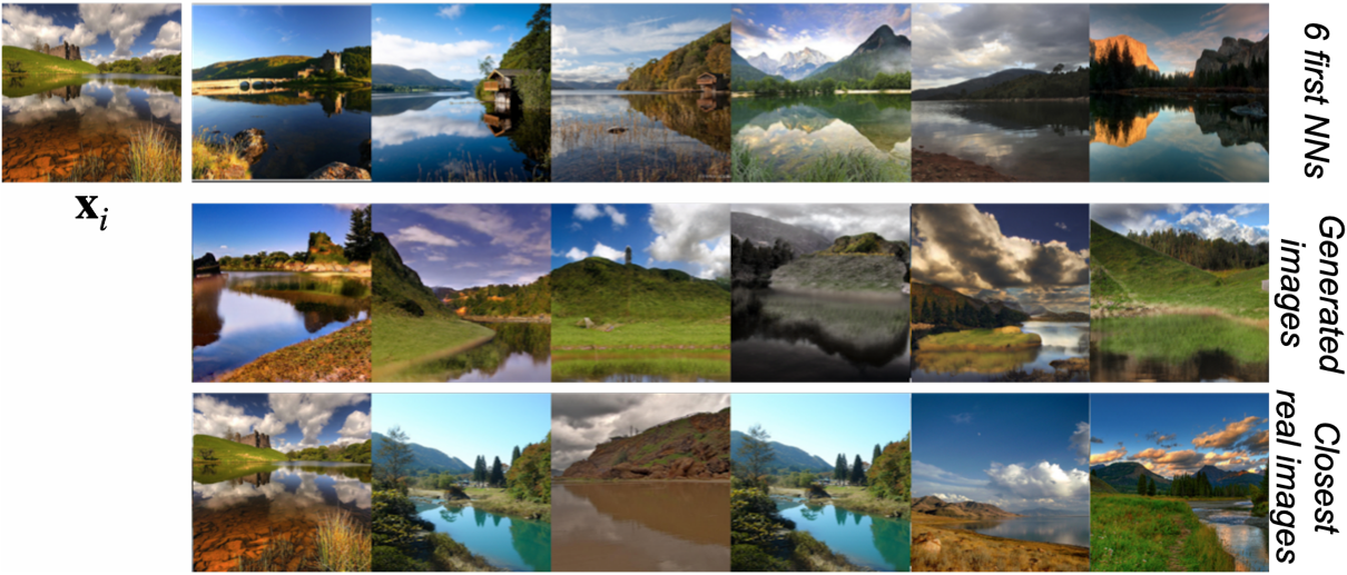
Figure 5: Qualitative results on unlabeled ImageNet ($256\!\times\!256$). Next to each input sample $\mathbf{x}_{i}$, used to obtain the instance features $\mathbf{h}_{i}\,=\,f_{\theta}(\mathbf{x}_{i})$, the six nearest neighbors in the feature space of $f_{\theta}$ are displayed. Below the neighbors, generated images sampled from IC-GAN with a BigGAN backbone and conditioned on $\mathbf{h}_{i}$ are depicted. Immediately below the generated images, the closest image in the ImageNet training set is shown for each example (cosine distance in the feature space of $f_{\theta}$).

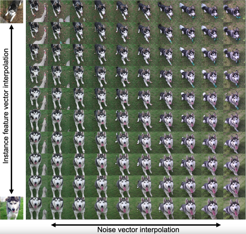
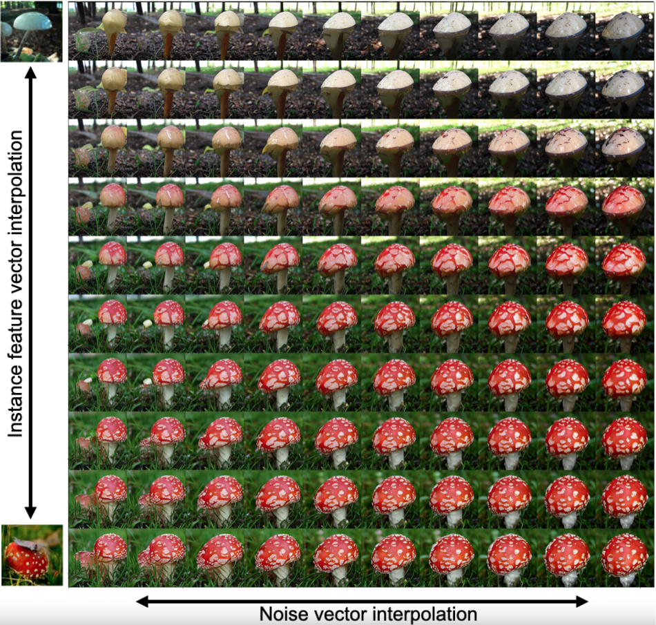
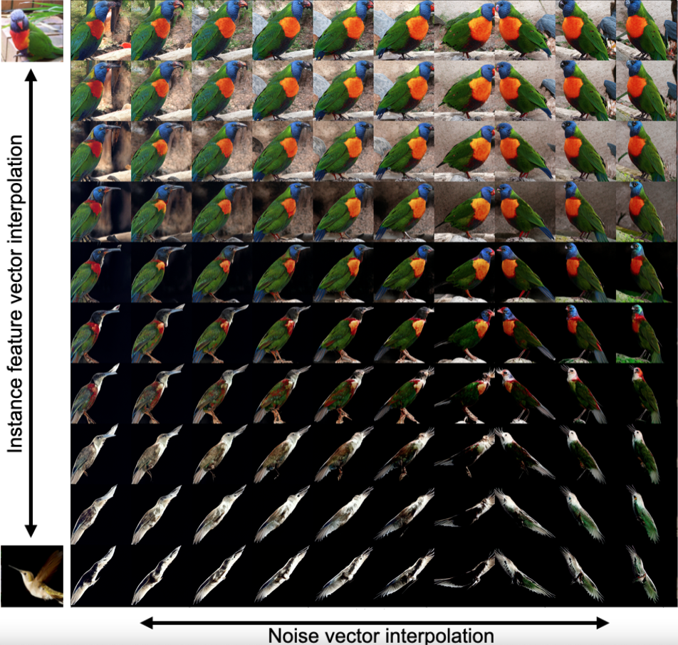
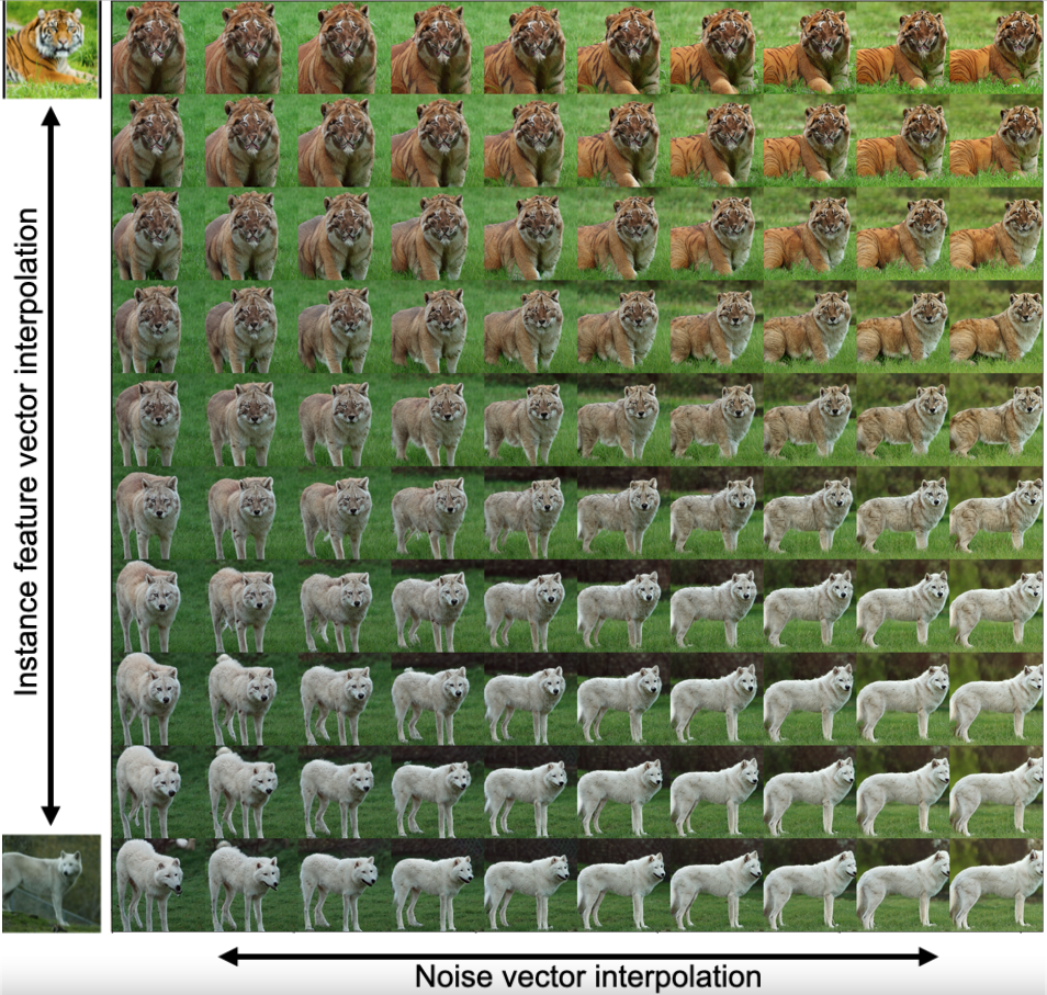
Figure 6: Qualitative results on unlabeled ImageNet ($256\!\times\!256$) using IC-GAN (BigGAN backbone) and interpolating between two instance feature vector conditionings (vertical axis) and two input noise vectors (horizontal axis).The two images depicted to the left of the generated image grids are used to extract the instance feature vectors used for the interpolation.

(a) $\mathbf{x}_{i}$

(b) LostGANv2 [49]

(c) OC-GAN [50]

(d) IC-GAN (StyleGAN2)

Figure 7: Qualitative comparison for scene generation on $256\!\times\!256$ COCO-Stuff with other state-of-the-art scene generation methods. (a) Data samples $\mathbf{x}_{i}$ from which instance features $\mathbf{h}_{i}\,=\,f(\mathbf{x}_{i})$ are obtained for IC-GAN, and labeled bounding box conditionings are obtained for LostGANv2 and OC-GAN. Images generated with two random seeds with (b) LostGANv2 [49], (c) OC-GAN [50], (d) IC-GAN (StyleGAN2).

ImageNet.

Class-conditional IC-GAN with a BigGAN backbone has shown comparable quantitative results to those of BigGAN for $256\!\times\!256$ resolution in Subsection 3.4. In Figure 8, we can qualitatively compare BigGAN ($ch\times 64$) (first rows) and IC-GAN ($ch\times 64$) (second and third rows), for three class labels: goldfish, limousine and red fox. By visually inspecting the generated images, we can observe that the generation quality is similar for both BigGAN and IC-GAN in these specific cases. Moreover, IC-GAN allows controllability of the semantics by changing the conditioning instance features. For instance, changing the background in which the goldfish are swimming into lighter colors in Figure 8(a), generating limousines in generally dark and uniform backgrounds or, instead, in an urban environment with a road and buildings (Figure 8(b)), or generating red foxes with a close up view or with a full body shot as seen in Figure 8(c).

Swapping classes for class-conditional IC-GAN on ImageNet.

In Figure 8, we show that we can change the appearance of the generated images by leveraging different instances of the same class. In Figure 9, we take a further step and condition on instance features from other classes. More specifically, in Figure 9 (top), we condition on the instance features of a snowplow in the woods surrounded by snow, and ask to generate snowplows, camels and zebras. Perhaps surprisingly, the generated images effectively get rid of the snowplow, and replace it by camel-looking and zebra-looking objects, respectively, while maintaining a snowy background in the woods. Moreover, when comparing the generated images with the closest samples in ImageNet, we see that for generated camels in the snow, the closest images are either a camel standing in dirt or other animals in the snow; for the generated zebras in the snow, we find one sample of a zebra standing in the snow, while others are standing in other locations/backgrounds. In Figure 9 (bottom), we condition on the features of an instance that depicts a golden retriever on a beach with overall purple tones, and ask to generate golden retrievers, camels or zebras. In most cases, generated images contain camels and zebras standing on water, while other generations contain purple or blue tones, similar to the instance used as conditioning. Note that, except one generated zebra image, the closest samples in ImageNet do not depict camels or zebras standing in the water nor on the beach.

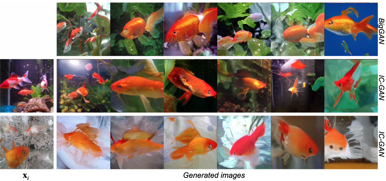
(a) Class label Goldfish

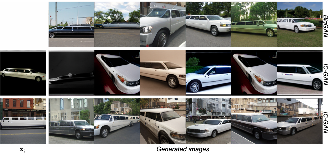
(b) Class label Limousine

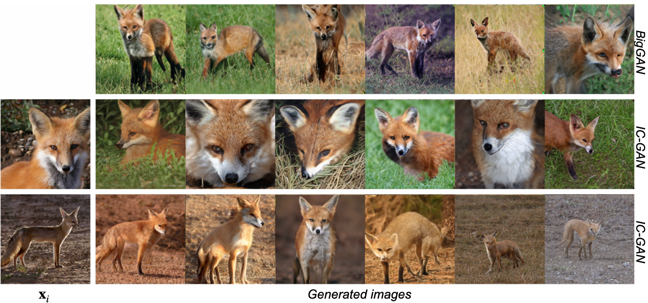
(c) Class label Red fox

Figure 8: Qualitative results in $256\!\times\!256$ ImageNet. For each class, generated images with BigGAN are presented in the first row, while the second and third row show generated images using class-conditional IC-GAN with a BigGAN backbone, conditioned on the instance feature extracted from the data sample to their left ($\mathbf{x}_{i}$) and their corresponding class.

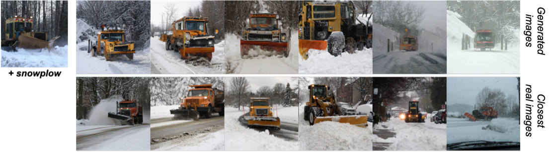
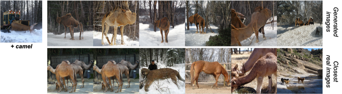
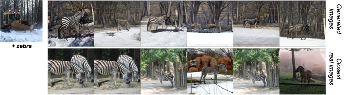
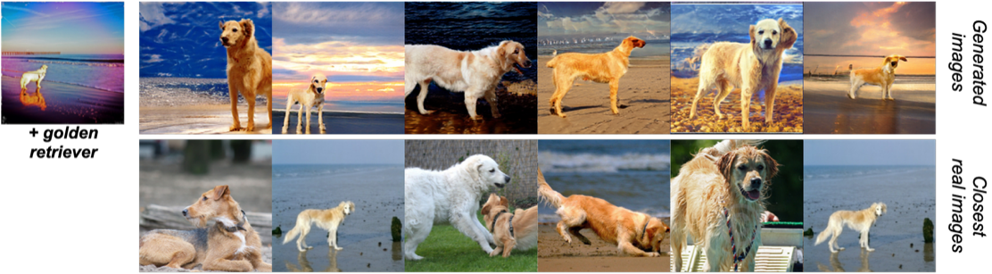
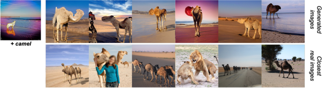
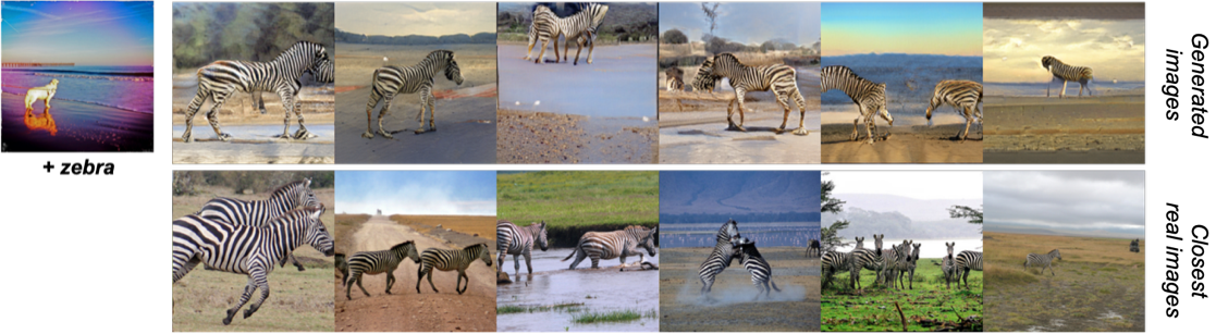
Figure 9: Generated $256\!\times\!256$ images with a class-conditional IC-GAN (BigGAN backbone) trained on ImageNet. Next to each data sample $\mathbf{x}_{i}$, used to obtain the instance features $\mathbf{h}_{i}\,=\,f_{\theta}(\mathbf{x}_{i})$, we find generated images sampled from IC-GAN using $\mathbf{h}_{i}$ and six sampled noise vectors. Below the generated images, the closest image in the ImageNet training set are shown (Cosine similarity in the feature space of $f_{\theta}$).

Appendix F Additional off-the-shelf transfer results for IC-GAN

Is IC-GAN able to shift the generated data distribution by conditioning on different instances?

As discussed in Section 3.3, we can transfer an IC-GAN trained on unlabeled ImageNet to COCO-Stuff and obtain better metrics and qualitative results than with the same IC-GAN trained on COCO-Stuff. We hypothesize that the success of this experiment comes from the flexibility of our conditioning strategy, where the generative model exploits the generalization capabilities of the feature extractor when dealing with unseen instances to shift the distribution of generated images from ImageNet to COCO-Stuff. To test this hypothesis we design the following experiment: we compute FID scores of generated images obtained by conditioning IC-GAN with instance features from either ImageNet or COCO-Stuff and use either COCO-Stuff or ImageNet as a reference dataset to compute FID. In Table 10 (first row) we show that when using COCO-Stuff for both the instance features and the reference dataset, IC-GAN scores 8.5 FID; this is a lower FID score than the 43.6 FID obtained in Table 10 (second row) when conditioning IC-GAN on ImageNet instance features and using COCO-Stuff as reference dataset. Moreover, when using COCO-Stuff instance features and ImageNet as reference dataset, in Table 10 (third row), we obtain 37.2 FID. This shows that, by changing the conditioning instance features, IC-GAN successfully exploits the generalization capabilities of the feature extractor to shift the distribution of generated images to be closer to the COCO-Stuff distribution. Additionally, note that the distance between ImageNet and COCO-Stuff datasets can be quantified with an FID score of 37.2 .

Table 10: FID scores on COCO-Stuff $128\!\times\!128$, when using an IC-GAN trained on ImageNet and tested with instance features from either COCO-Stuff or ImageNet and using either of those datasets as reference. The metrics obtained by sampling $1,\!000$ instance features (k-means) from either ImageNet or COCO, and generating $76,\!000$ samples. As a reference, $76,\!000$ real samples from COCO-Stuff or ImageNet training set are used.

	train instance dataset	eval instance dataset	FID reference dataset	$\downarrow$FID
IC-GAN	ImageNet	COCO-Stuff	COCO-Stuff	8.5 $\pm$ 0.1
IC-GAN	ImageNet	ImageNet	COCO-Stuff	43.6 $\pm$ 0.1
IC-GAN	ImageNet	COCO-Stuff	ImageNet	37.2 $\pm$ 0.1

What is being transferred when IC-GAN is conditioned on instances other than the ones in the training dataset?

From the point of view of KDE, what is being transferred is the kernel shape, not the kernel location (that is controlled by instances). The kernel shape is predicted using a generative model from each input instance and we probe the kernel via sampling from the generator. Thus, we transfer a function that predicts kernel shape from a conditioning, and this function seems to be robust to diverse instances as shown in the paper (e.g. see Figure 1(c) and 1(d)). Moreover, by visually inspecting the generated images in our transfer experiments, we observed that when transferring an IC-GAN trained on ImageNet to COCO-Stuff, if the model is conditioned on images that contain unseen classes in ImageNet, such as “giraffe”, the model will still generate an animal that would look like a giraffe without the skin patterns and characteristic antennae, because ImageNet contains other animals to draw inspiration from. This suggests that the model generates plausible images that have some similar features to those present in the instance conditioning, but adapting it to the training dataset style. Along these lines, we also observed that in some cases, shapes and other object characteristics from one dataset are transferred to another (ImageNet to COCO-Stuff). Moreover, when we conditioned on instances from Cityscapes, the generated images were rather colorful, resembling more the color palette of ImageNet images rather than the Cityscapes one.

Off-the-shelf transfer results for IC-GAN.

In Figure 10, we provide additional generated samples and their closest images in the ImageNet training set, when conditioning on unseen instance features from other datasets. Generated images often differ substantially from the closest image in ImageNet. Although generated images using a COCO-Stuff and Cityscapes instances may have somewhat similar looking images in ImageNet (for the first and second instances in Figure 10), the differences accentuate when conditioning on instance features from MetFaces, PACS or Sketch datasets, where, for instance, IC-GAN with a BigGAN backbone generates images resembling sketch strokes in the last row, even if the closest ImageNet samples depict objects that are not sketches.

Off-the-shelf transfer results for class-conditional IC-GAN.

In Figure 11, we show additional results when transferring a class-conditional IC-GAN with a BigGAN backbone trained on ImageNet to other datasets, using an ImageNet class label but an unseen instance. We are able to generate camels in the grass by conditioning on an image of a cow in the grass from COCO-Stuff, we show generated images with a zebra in an urban environment by conditioning on a Cityscapes instance, and we generate cartoon-ish birdhouses by conditioning on a PACS cartoon house instance. This highlights the ability of class-conditional IC-GAN to transfer to other datasets styles while maintaining the class label semantics.

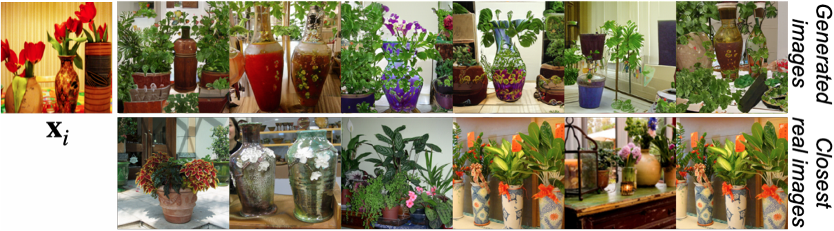
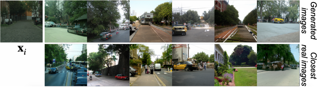
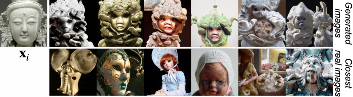
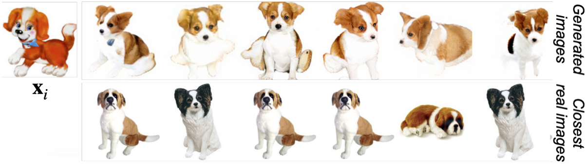
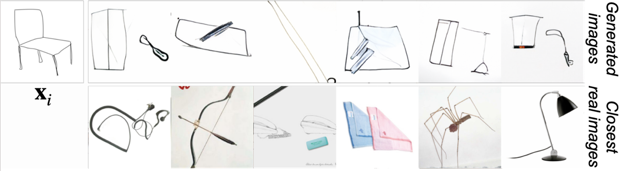
Figure 10: Qualitative off-the-shelf transfer results in $256\!\times\!256$, using an IC-GAN trained on unlabeled ImageNet and conditioning on unseen instances from other datasets. The instances come from the following datasets (top to bottom): COCO-Stuff, Cityscapes, MetFaces, PACS (cartoons), Sketches. Next to each data sample $\mathbf{x}_{i}$, used to obtain the instance features $\mathbf{h}_{i}\,=\,f_{\theta}(\mathbf{x}_{i})$, generated images conditioning on $\mathbf{h}_{i}$ are displayed. Immediately below each generated image, the closest image in the ImageNet training set is displayed (Euclidean distance in the feature space of $f_{\theta}$).

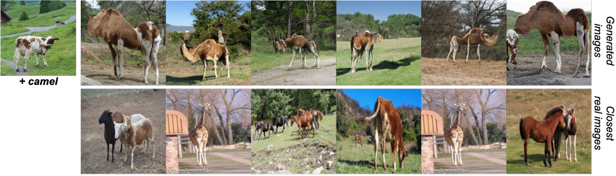
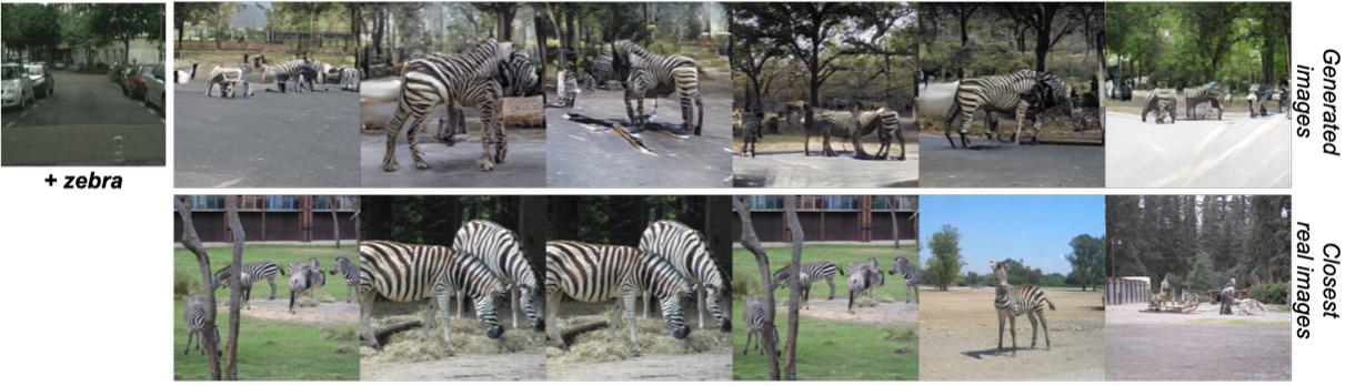
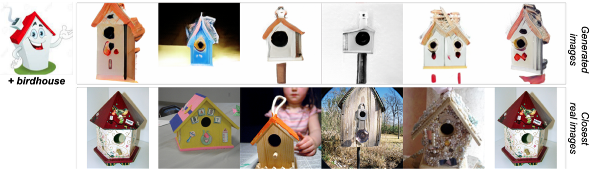
Figure 11: Qualitative off-the-shelf transfer results in $256\!\times\!256$, using a class-conditional IC-GAN trained on ImageNet and conditioning on unseen instances from other datasets and a class label. The instances come from the following datasets (top to bottom): COCO-Stuff, Cityscapes, PACS (cartoons). On the left, a data sample $\mathbf{x}_{i}$ is depicted, used to obtain the instance features $\mathbf{h}_{i}\,=\,f_{\theta}(\mathbf{x}_{i})$. Next to the data samples, generated images conditioning on $\mathbf{h}_{i}$ and a class label (under the data samples) are displayed. Just below the generated images, the closest image in the ImageNet training set are shown (Euclidean distance in the feature space of $f_{\theta}$).

Appendix G Class balancing in ImageNet-LT

We experimented with class balancing for BigGAN in the ImageNet-LT dataset. In Table 11, we compare (1) BigGAN, where both the class distribution for the generator and the data for the discriminator are long-tailed; (2) BigGAN (CB), a class-balanced version of BigGAN, where the generator samples class labels from a uniform distribution and the samples fed to the discriminator are also class-balanced; and (3) BigGAN (T = 2) where the class distribution is balanced with a softmax temperature of T = 2 providing a middle ground between the long-tail and the uniform distributions. In the latter case, the probability to sample class $c$ (with a frequency $f_{c}$ in the long-tailed training set) during training is given by $p_{c}\,=\,\text{softmax}(T^{-1}\ln f_{c})$.

Interestingly, balancing the class distribution (either with uniform class distribution or with T=2) harmed performance in all cases except for the validation Inception Score. We hypothesize that oversampling rare classes, and thus the few images therein, may result in overfitting for the discriminator, leading to low quality image generations.

Table 11: ImageNet-LT quantitative results for different class balancing techniques. "t.": training and "v.": validation.

	Res.	$\downarrow$t. FID	$\uparrow$t. IS	$\downarrow$v. FID	$\downarrow$v. [many/med/few] FID	$\uparrow$v. IS
BigGAN	64	27.6 $\pm$ 0.1	18.1 $\pm$ 0.2	28.1 $\pm$ 0.1	28.8/32.8/48.4 $\pm$ 0.2	16.0 $\pm$ 0.1
BigGAN (CB)	64	62.1 $\pm$ 0.1	10.7 $\pm$ 0.2	56.2 $\pm$ 0.1	62.2/59.7/74.7 $\pm$ 0.2	11.0 $\pm$ 0.0
BigGAN (T = 2)	64	30.6 $\pm$ 0.1	16.8 $\pm$ 0.1	29.2 $\pm$ 0.1	30.9/33.3/49.5 $\pm$ 0.2	16.4 $\pm$ 0.1

Appendix H Choice of feature extractor

We study the choice of the feature extractor used to obtain instance features in Table 12. We compare results using an IC-GAN with a BigGAN backbone when coupling it with a ResNet50 feature extractor trained with either self supervision (SwAV) or with supervision for classification purposes (RN50) on ImageNet dataset. Results highlight similar IC-GAN performances for both feature extractors, suggesting that the choice of feature extractor that does not greatly impact the performance of our method when leveraging unlabeled datasets. Given that for the unlabeled scenario we assume no labels are available, we use the SwAV feature extractor. However, in the class-conditional case, we observe that the IC-GAN coupled with a RN50 feature extractor surpasses IC-GAN coupled with a SwAV feature extractor. Therefore, we choose the RN50 feature extractor for the class-conditional experiments. For ImageNet-LT, we transfer these findings and use a RN50 trained on ImageNet-LT as feature extractor, assuming we do not have access to the entire ImageNet dataset and its labels.

Table 12: Feature extractor impact with SwAV (ResNet50 trained with a self-supervised approach) and RN50 (ResNet50 trained for the classification task in ImageNet). Experiments performed in $64\!\times\!64$ ImageNet, using $1,\!000$ training instance features at test time, selected with k-means.

	$\downarrow$FID
IC-GAN + SwAV	11.7 $\pm$ 0.1
IC-GAN + RN50	11.3 $\pm$ 0.1
Class-conditional IC-GAN + SwAV	9.9 $\pm$ 0.1
Class-conditional IC-GAN + RN50	8.5 $\pm$ 0.0

Appendix I Number of conditioning instance features at train time

To demonstrate that using many fine-grained overlapping partitions results in better performance than using a few coarser partitions, we trained IC-GAN with a BigGAN backbone by conditioning on all 1.2M training instance features at training time in ImageNet and a neighborhood size of $k\,=\,50$, and compared it quantitatively with an IC-GAN trained by conditioning on only $1,\!000$ instance features at training time. In this case, we extend the neighborhood size to $k\,=\,1,\!200$ to better cover the training distribution . Note that using $k\,=\,50$ would result in using at most $50,\!000$ training samples during training, an unfair comparison. The $1,\!000$ instance features are selected by applying k-means to the entire ImageNet training set. We then use the same instances to generate images. Results are presented in Table 13 and emphasize the importance of training with all available instances, which results in significantly better FID and IS presumably due to the increased number of conditionings and their smaller neighborhoods.

Table 13: Comparison between training IC-GAN (BigGAN backbone) using only $1,\!000$ conditioning instance features (selected with k-means) or all training instance features during training, in IC-GAN $64\!\times\!64$. At test time, we condition IC-GAN on $1,\!000$ training instance features, selected with k-means.

Method	$\downarrow$FID	$\uparrow$IS
IC-GAN ($k\,=\,50$, trained with all 1.2M conditionings)	11.7 $\pm$ 0.1	21.6 $\pm$ 0.1
IC-GAN ($k\,=\,1,\!200$, trained with only $1,\!000$ conditionings)	24.8 $\pm$ 0.1	16.4 $\pm$ 0.1

Appendix J Matching storage requirements for IC-GAN and unconditional models

We hypothesize that the good performance of IC-GAN on ImageNet and COCO-Stuff can not solely be attributed to the slight increase of parameters and the extra memory required to store the instance features used at test time, but also to the IC-GAN design, including the finegrained overlapping partitions and the instance conditionings. To test for this hypothesis, we performed experiments with the unconditional BigGAN baseline on ImageNet and COCO-Stuff, training it by setting all labels in the training set to zero, following [36, 42], and increasing the generator capacity such that it matches the IC-GAN storage requirements. In particular, we not only endowed the unconditional BigGAN with additional parameters to compensate for the capacity mismatch, but also for the instances required by IC-GAN. Moreover, we performed analogous experiments for the unconditional StyleGAN2 in COCO-Stuff.

ImageNet.

Given its instance conditioning, the IC-GAN (BigGAN backbone) generator introduces an additional 4.5M parameters when compared to the unconditional BigGAN generator. Moreover, IC-GAN requires an extra 8MB to store the $1,\!000$ instance features used at inference time. This 8MB can be translated into roughly 2M parameters. Therefore, we compensate for this additional storage in IC-GAN by increasing the unconditional BigGAN capacity by expanding the width of both generator and discriminator hidden layers. We follow the practice in [5], where the generator and discriminator’s width are changed together. The resulting unconditional BigGAN baseline generator has an additional 6.5M parameters. Results are reported in Table 14, showing that adding extra capacity to the unconditional BigGAN leads to an improvement in terms of FID and IS. However, IC-GAN still exhibits significantly better FID and IS, highlighting that the improvements cannot be solely attributed to the increase in parameters nor instance feature storage requirements.

COCO-Stuff.

Similarly, IC-GAN (BigGAN backbone) trained on COCO-Stuff requires 4M additional parameters on top of the extra storage required by the $1,\!000$ stored instance features (8MB again translated into roughly 2M parameters). Therefore, we add 6M extra parameters to the unconditional BigGAN generator. In the case of IC-GAN with a StyleGAN2 backbone, the instance feature conditionings constitute 1M additional parameters. We therefore increase the capacity of the unconditional StyleGAN2 model by 3M to match the storage requirements of IC-GAN (StyleGAN2 backbone). The results are presented in Table 15, where it is shown that both the unconditional BigGAN and unconditional StyleGAN2 do not take advantage of the additional capacity and achieve poorer performance than the model with lower capacity, possibly due to overfitting. When compared to IC-GAN, the results match the findings in the ImageNet dataset: IC-GAN exhibits lower FID when using BigGAN or StyleGAN2 backbones, compared to their respective unconditional models with the same storage requirements, further highlighting that IC-GAN effectively benefits from its design, finegrained overlapping partitions, and instance conditionings.

Table 14: Comparing IC-GAN with the unconditional counterparts of BigGAN on $64\!\times\!64$ ImageNet with the same storage requirements. Storage-G counts the storage required for the generator, Storage-I the storage required for the training instance features, and Storage-All is the sum of both generator and instance features required storage. FID and IS scores are computed using Pytorch code.

Method	#prms.	Storage-G	Storage-I	Storage-All	$\downarrow$FID	$\uparrow$IS
Unconditional BigGAN	32.5M	124MB	0MB	124MB	30.0 $\pm$ 0.1	12.1 $\pm$ 0.1
Unconditional BigGAN	39M	149MB	0MB	149MB	16.9 $\pm$ 0.0	14.6 $\pm$ 0.1
IC-GAN (BigGAN)	37M	141MB	8MB	149MB	10.4 $\pm$ 0.1	21.9 $\pm$ 0.1

Table 15: Comparing IC-GAN with the unconditional counterparts on $128\!\times\!128$ COCO-Stuff, with the same storage requirements. Storage-G counts the storage required for the generator, Storage-I the storage required for the training instance features, and Storage-All is the sum of both generator and instance features required storage.

	#prms.	Storage-G	Storage-I	Storage-All	$\downarrow$FID
					train	eval
Unconditional BigGAN	18M	68MB	0MB	68MB	17.9 $\pm$ 0.1	46.9 $\pm$ 0.5
Unconditional BigGAN	24M	92MB	0MB	92MB	28.8 $\pm$ 0.1	58.1 $\pm$ 0.5
IC-GAN (BigGAN)	22M	84MB	8MB	92MB	16.8 $\pm$ 0.1	44.9 $\pm$ 0.5
Unconditional StyleGAN2	23M	88MB	0MB	88MB	8.8 $\pm$ 0.1	37.8 $\pm$ 0.2
Unconditional StyleGAN2	26M	100MB	0MB	100MB	9.4 $\pm$ 0.0	38.4 $\pm$ 0.3
IC-GAN (StyleGAN2)	24M	92MB	8MB	100MB	8.7 $\pm$ 0.0	35.8 $\pm$ 0.1

Appendix K Additional neighborhood size impact studies

We additionally study the impact of the neighborhood size for ImageNet-LT in Table 16 and in COCO-Stuff in Table 17, showing that in both cases, IC-GAN with a BigGAN backbone and $k\,=\,5$ achieves the best FID and IS metrics. The choice of a lower neighborhood size $k\,=\,5$ than in the ImageNet case ($k\,=\,50$) could suggest that the number of semantically similar neighboring samples is smaller for these two datasets. This wouldn’t be completely surprising given that these two datasets are considerably smaller than ImageNet. Increasing the value of $k$ in COCO-Stuff and ImageNet-LT would potentially gather samples with different semantics within a neighborhood, which could potentially harm the training and therefore the generated images quality.

Finally, in Figure 12, we qualitatively show generated images in ImageNet when using an IC-GAN trained with varying neighborhood sizes. The findings further support the ones presented in Subsection 3.5, showing that smaller neighborhoods result in generated images with less diversity, while bigger neighborhood sizes, for example $k\,=\,500$ result in more varied but lower quality generations, supporting that $k$ controls the smoothing effect.

Table 16: Impact of the number of neighbors ($k$) used to train class-conditional IC-GAN (BigGAN backbone) in ImageNet-LT $64\!\times\!64$. Reported results in ImageNet validation set. As a feature extractor, a ResNet50 is trained as a classifier on the same dataset is used. 50k instance features are sampled from the training set.

	$\downarrow$FID	$\uparrow$IS
$k$ = 5	23.4 $\pm$ 0.1	17.6 $\pm$ 0.1
$k$ = 20	24.1 $\pm$ 0.1	16.8 $\pm$ 0.1
$k$ = 50	24.1 $\pm$ 0.1	16.7 $\pm$ 0.1
$k$ = 100	25.6 $\pm$ 0.1	16.3 $\pm$ 0.1
$k$ = 500	27.1 $\pm$ 0.1	15.3 $\pm$ 0.1

Table 17: Impact of the number of neighbors ($k$) used to train IC-GAN (BigGAN backbone) on COCO-Stuff $128\!\times\!128$. Reported results on COCO-Stuff evaluation set. As a feature extractor, a ResNet50 trained with self-supervision (SwAV) is used.

	$\downarrow$FID
$k$ = 5	44.9 $\pm$ 0.5
$k$ = 20	46.8 $\pm$ 0.3
$k$ = 50	45.8 $\pm$ 0.4
$k$ = 100	48.4 $\pm$ 0.3
$k$ = 500	48.3 $\pm$ 0.5

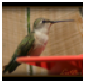
(a) $\mathbf{x}_{i}$

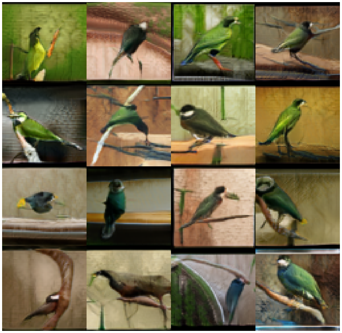
(b) IC-GAN trained with $k\!=\!5$

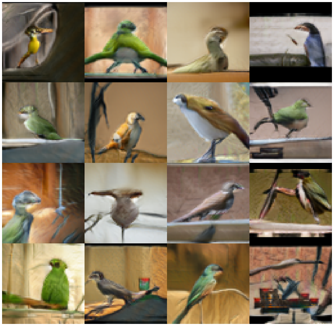
(c) IC-GAN trained with $k\!=\!20$

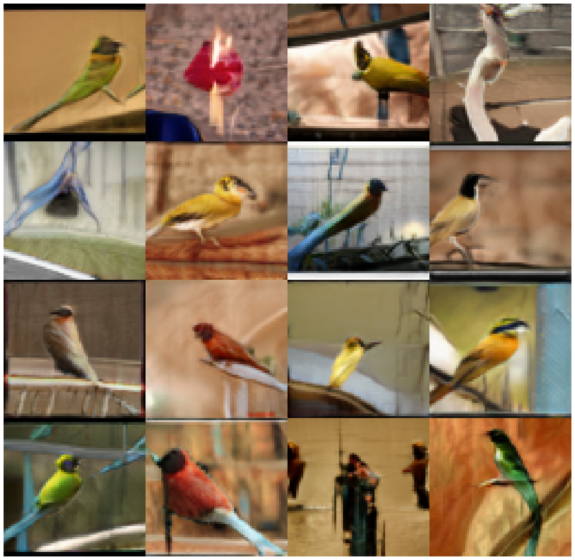
(d) IC-GAN trained with $k\!=\!50$

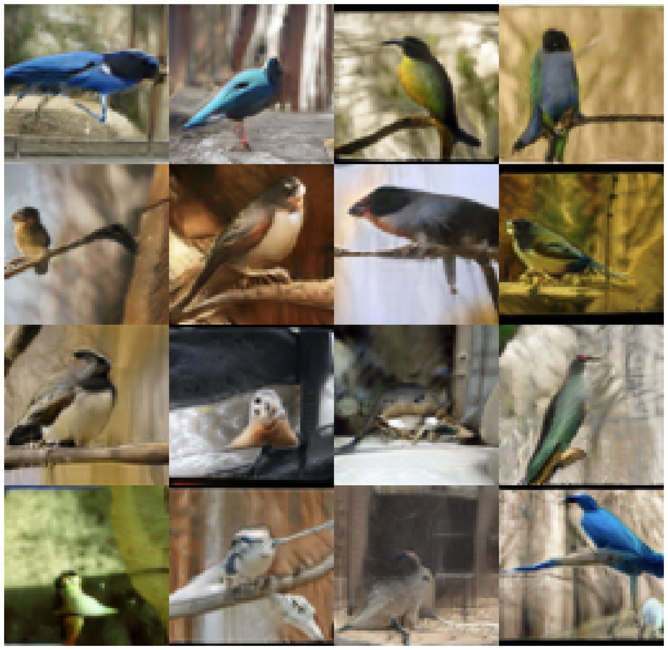
(e) IC-GAN trained with $k\!=\!100$

(f) IC-GAN trained with $k\!=\!500$

Figure 12: Qualitative results in $64\!\times\!64$ unlabeled ImageNet when training IC-GAN (BigGAN backbone) with different neighborhood sizes $k$. (a) Data samples $\mathbf{x}_{i}$ used to obtain the instance features $\mathbf{h}_{i}\,=\,f_{\theta}(\mathbf{x}_{i})$. (b-f) Generated images with IC-GAN (BigGAN backbone), sampling different noise vectors, for different neighborhood sizes $k$ used during training.

References

- Abbasnejad et al. [2019] M Ehsan Abbasnejad, Qinfeng Shi, Anton van den Hengel, and Lingqiao Liu. A generative adversarial density estimator. In CVPR, 2019.
- Armandpour et al. [2021] Mohammadreza Armandpour, Ali Sadeghian, Chunyuan Li, and Mingyuan Zhou. Partition-guided GANs. arXiv preprint, (arXiv:2104.00816), 2021.
- Ashual and Wolf [2019] Oron Ashual and Lior Wolf. Specifying object attributes and relations in interactive scene generation. In CVPR, 2019.
- Bishop [2006] C. Bishop. Pattern recognition and machine learning. Spinger-Verlag, 2006.
- [5] Andrew Brock, Jeff Donahue, and Karen Simonyan. Large scale GAN training for high fidelity natural image synthesis. In ICLR. URL https://openreview.net/forum?id=B1xsqj09Fm.
- Caesar et al. [2018] Holger Caesar, Jasper Uijlings, and Vittorio Ferrari. COCO-Stuff: Thing and stuff classes in context. In CVPR, 2018.
- Caron et al. [2020] Mathilde Caron, Ishan Misra, Julien Mairal, Priya Goyal, Piotr Bojanowski, and Armand Joulin. Unsupervised learning of visual features by contrasting cluster assignments. In NeurIPS, 2020.
- Casanova et al. [2020] Arantxa Casanova, Michal Drozdzal, and Adriana Romero-Soriano. Generating unseen complex scenes: are we there yet? arXiv preprint, (arXiv:2012.04027), 2020.
- Chen and Koltun [2017] Qifeng Chen and Vladlen Koltun. Photographic image synthesis with cascaded refinement networks. In CVPR, 2017.
- Cordts et al. [2016] Marius Cordts, Mohamed Omran, Sebastian Ramos, Timo Rehfeld, Markus Enzweiler, Rodrigo Benenson, Uwe Franke, Stefan Roth, and Bernt Schiele. The cityscapes dataset for semantic urban scene understanding. In CVPR, 2016.
- DeVries et al. [2020] Terrance DeVries, Michal Drozdzal, and Graham W. Taylor. Instance selection for GANs. In NeurIPS, 2020.
- Dhariwal and Nichol [2021] Prafulla Dhariwal and Alex Nichol. Diffusion models beat GANs on image synthesis. arXiv preprint, (arXiv:2105.05233), 2021.
- Dolhansky et al. [2019] Brian Dolhansky, Russ Howes, Ben Pflaum, Nicole Baram, and Cristian Canton-Ferrer. The deepfake detection challenge (DFDC) preview dataset. CoRR, abs/1910.08854, 2019. URL http://arxiv.org/abs/1910.08854.
- Eghbal-zadeh et al. [2019] Hamid Eghbal-zadeh, Werner Zellinger, and Gerhard Widmer. Mixture density generative adversarial networks. In CVPR, 2019.
- Eitz et al. [2012] Mathias Eitz, James Hays, and Marc Alexa. How do humans sketch objects? ACM Trans. Graph. (Proc. SIGGRAPH), 31(4):44:1–44:10, 2012.
- Gao et al. [2020] Chengying Gao, Qi Liu, Qi Xu, Limin Wang, Jianzhuang Liu, and Changqing Zou. SketchyCOCO: image generation from freehand scene sketches. In CVPR, 2020.
- Ghosh et al. [2018] Arnab Ghosh, Viveka Kulharia, Vinay P. Namboodiri, Philip H.S. Torr, and Puneet K. Dokania. Multi-agent diverse generative adversarial networks. In CVPR, 2018.
- Goodfellow et al. [2014] Ian J Goodfellow, Jean Pouget-Abadie, Mehdi Mirza, Bing Xu, David Warde-Farley, Sherjil Ozair, Aaron Courville, and Yoshua Bengio. Generative adversarial networks. In NeurIPS, 2014.
- Grinblat et al. [2017] Guillermo L Grinblat, Lucas C Uzal, and Pablo M Granitto. Class-splitting generative adversarial networks. arXiv preprint, (arXiv:1709.07359), 2017.
- Gulrajani et al. [2017] Ishaan Gulrajani, Faruk Ahmed, Martin Arjovsky, Vincent Dumoulin, and Aaron Courville. Improved training of Wasserstein GANs. In NeurIPS, 2017.
- He et al. [2016] Kaiming He, Xiangyu Zhang, Shaoqing Ren, and Jian Sun. Deep residual learning for image recognition. In CVPR, 2016.
- Heusel et al. [2017] Martin Heusel, Hubert Ramsauer, Thomas Unterthiner, Bernhard Nessler, and Sepp Hochreiter. GANs trained by a two time-scale update rule converge to a local Nash equilibrium. In NeurIPS, 2017.
- Hoang et al. [2018] Quan Hoang, Tu Dinh Nguyen, Trung Le, and Dinh Phung. MGAN: Training generative adversarial nets with multiple generators. In ICLR, 2018.
- Johnson et al. [2017] Jeff Johnson, Matthijs Douze, and Hervé Jégou. Billion-scale similarity search with gpus. arXiv preprint arXiv:1702.08734, 2017.
- Johnson et al. [2018] Justin Johnson, Agrim Gupta, and Li Fei-Fei. Image generation from scene graphs. In CVPR, 2018.
- Kang et al. [2020] Bingyi Kang, Saining Xie, Marcus Rohrbach, Zhicheng Yan, Albert Gordo, Jiashi Feng, and Yannis Kalantidis. Decoupling representation and classifier for long-tailed recognition. In ICLR, 2020.
- Karras et al. [2019] Tero Karras, Samuli Laine, and Timo Aila. A style-based generator architecture for generative adversarial networks. In CVPR, 2019.
- Karras et al. [2020a] Tero Karras, Miika Aittala, Janne Hellsten, Samuli Laine, Jaakko Lehtinen, and Timo Aila. Training generative adversarial networks with limited data. In NeurIPS, 2020a.
- Karras et al. [2020b] Tero Karras, Samuli Laine, Miika Aittala, Janne Hellsten, Jaakko Lehtinen, and Timo Aila. Analyzing and improving the image quality of StyleGAN. In CVPR, 2020b.
- Kynkäänniemi et al. [2019] Tuomas Kynkäänniemi, Tero Karras, Samuli Laine, Jaakko Lehtinen, and Timo Aila. Improved precision and recall metric for assessing generative models. arXiv preprint arXiv:1904.06991, 2019.
- Li et al. [2017] Da Li, Yongxin Yang, Yi-Zhe Song, and Timothy M Hospedales. Deeper, broader and artier domain generalization. In CVPR, 2017.
- Lin et al. [2018] Zinan Lin, Ashish Khetan, Giulia Fanti, and Sewoong Oh. PacGAN: The power of two samples in generative adversarial networks. In NeurIPS, 2018.
- Liu et al. [2020] Steven Liu, Tongzhou Wang, David Bau, Jun-Yan Zhu, and Antonio Torralba. Diverse image generation via self-conditioned GANs. In CVPR, 2020.
- Liu et al. [2019] Ziwei Liu, Zhongqi Miao, Xiaohang Zhan, Jiayun Wang, Boqing Gong, and Stella X. Yu. Large-scale long-tailed recognition in an open world. In CVPR, 2019.
- Lucas et al. [2018] T. Lucas, C. Tallec, Y. Ollivier, and J. Verbeek. Mixed batches and symmetric discriminators for GAN training. In ICML, 2018.
- Lučić et al. [2019] Mario Lučić, Michael Tschannen, Marvin Ritter, Xiaohua Zhai, Olivier Bachem, and Sylvain Gelly. High-fidelity image generation with fewer labels. In ICML, 2019.
- Mangla et al. [2022] Puneet Mangla, Nupur Kumari, Mayank Singh, Balaji Krishnamurthy, and Vineeth N. Balasubramanian. Data instance prior (DISP) in generative adversarial networks. WACV, 2022.
- Metz et al. [2016] Luke Metz, Ben Poole, David Pfau, and Jascha Sohl-Dickstein. Unrolled generative adversarial networks. arXiv preprint, (arXiv:1611.02163), 2016.
- Mirza and Osindero [2014] Mehdi Mirza and Simon Osindero. Conditional generative adversarial nets. arXiv preprint, (arXiv:1411.1784), 2014.
- Miyato et al. [2018] Takeru Miyato, Toshiki Kataoka, Masanori Koyama, and Yuichi Yoshida. Spectral normalization for generative adversarial networks. arXiv preprint, (arXiv:1802.05957), 2018.
- Naeem et al. [2020] Muhammad Ferjad Naeem, Seong Joon Oh, Youngjung Uh, Yunjey Choi, and Jaejun Yoo. Reliable fidelity and diversity metrics for generative models. In ICML, 2020.
- Noroozi [2020] Mehdi Noroozi. Self-labeled conditional GANs. arXiv preprint, (arXiv:2012.02162), 2020.
- Park et al. [2019] Taesung Park, Ming-Yu Liu, Ting-Chun Wang, and Jun-Yan Zhu. Semantic image synthesis with spatially-adaptive normalization. In CVPR, 2019.
- Qi et al. [2018] Xiaojuan Qi, Qifeng Chen, Jiaya Jia, and Vladlen Koltun. Semi-parametric image synthesis. In CVPR, 2018.
- Russakovsky et al. [2015] Olga Russakovsky, Jia Deng, Hao Su, Jonathan Krause, Sanjeev Satheesh, Sean Ma, Zhiheng Huang, Andrej Karpathy, Aditya Khosla, Michael Bernstein, Alexander C. Berg, and Li Fei-Fei. ImageNet Large Scale Visual Recognition Challenge. International Journal of Computer Vision, 115(3):211–252, 2015. doi: 10.1007/s11263-015-0816-y.
- Sage et al. [2018] Alexander Sage, Eirikur Agustsson, Radu Timofte, and Luc Van Gool. Logo synthesis and manipulation with clustered generative adversarial networks. In CVPR, 2018.
- Salimans et al. [2016] T. Salimans, I. Goodfellow, W. Zaremba, V. Cheung, A. Radford, and X. Chen. Improved techniques for training GANs. In NeurIPS, 2016.
- Sun and Wu [2019] Wei Sun and Tianfu Wu. Image synthesis from reconfigurable layout and style. In CVPR, 2019.
- Sun and Wu [2020] Wei Sun and Tianfu Wu. Learning layout and style reconfigurable GANs for controllable image synthesis. arXiv preprint, (arXiv:2003.11571), 2020.
- Sylvain et al. [2020] Tristan Sylvain, Pengchuan Zhang, Yoshua Bengio, R Devon Hjelm, and Shikhar Sharma. Object-centric image generation from layouts. arXiv preprint, (arXiv:2003.07449), 2020.
- Szegedy et al. [2016] C. Szegedy, V. Vanhoucke, S. Ioffe, J. Shlens, and Z. Wojna. Rethinking the inception architecture for computer vision. In CVPR, 2016.
- Tang et al. [2020] Hao Tang, Dan Xu, Yan Yan, Philip HS Torr, and Nicu Sebe. Local class-specific and global image-level generative adversarial networks for semantic-guided scene generation. In CVPR, 2020.
- Touvron et al. [2020] Hugo Touvron, Alexandre Sablayrolles, Matthijs Douze, Matthieu Cord, and Hervé Jégou. Grafit: Learning fine-grained image representations with coarse labels. arXiv preprint, (arXiv:2011.12982), 2020.
- Vinyals et al. [2016] Oriol Vinyals, Charles Blundell, Timothy Lillicrap, Koray Kavukcuoglu, and Daan Wierstra. Matching networks for one shot learning. In NeurIPS, 2016. URL https://arxiv.org/abs/1606.04080.
- Wang et al. [2018] Ting-Chun Wang, Ming-Yu Liu, Jun-Yan Zhu, Andrew Tao, Jan Kautz, and Bryan Catanzaro. High-resolution image synthesis and semantic manipulation with conditional GANs. In CVPR, 2018.
- Zhang et al. [2019] Han Zhang, Ian Goodfellow, Dimitris Metaxas, and Augustus Odena. Self-attention generative adversarial networks. In ICML, 2019.
- Zhang et al. [2018] Richard Zhang, Phillip Isola, Alexei A Efros, Eli Shechtman, and Oliver Wang. The unreasonable effectiveness of deep features as a perceptual metric. In CVPR, 2018.
- Zhao et al. [2019] Bo Zhao, Lili Meng, Weidong Yin, and Leonid Sigal. Image generation from layout. In CVPR, 2019.
- Zhao et al. [2020] Shengyu Zhao, Zhijian Liu, Ji Lin, Jun-Yan Zhu, and Song Han. Differentiable augmentation for data-efficient GAN training. In NeurIPS, 2020.