The Speed–Robustness Trade-Off for First-Order Methods
with Additive Gradient Noise

Abstract

We study the trade-off between convergence rate and sensitivity to stochastic additive gradient noise for first-order optimization methods. Ordinary Gradient Descent (GD) can be made fast-and-sensitive or slow-and-robust by increasing or decreasing the stepsize, respectively. However, it is not clear how such a trade-off can be navigated when working with accelerated methods such as Polyak’s Heavy Ball (HB) or Nesterov’s Fast Gradient (FG) methods, or whether any of these methods can achieve an optimal trade-off. We consider three classes of functions: (1) strongly convex quadratics, (2) smooth strongly convex functions, and (3) nonconvex functions that satisfy a weak notion of strong convexity. For each function class, we present a tractable way to compute convergence rate and sensitivity to additive gradient noise for a broad family of first-order methods, and we present near-Pareto-optimal algorithm designs. Each design consists of a simple analytic update rule with two states of memory, similar to HB and FG. Moreover, each design has a scalar tuning parameter that explicitly trades off convergence rate and sensitivity to additive gradient noise. When tuned as aggressively as possible, our proposed algorithms recover the algorithms with fastest-known convergence rates for each function class. When tuned to be more robust, our algorithms are novel and provide a practical way to control noise sensitivity while maintaining the fastest possible convergence rate. We validate the performance and near-optimality of our designs through numerous numerical simulations.

1 Introduction

We consider the problem of designing robust first-order methods for unconstrained minimization. Given a differentiable function $f:\mathbb{R}^{d}\to\mathbb{R}$, consider solving the optimization problem

$$x^{\star}\in\operatorname*{\arg\min}_{x\in\mathbb{R}^{d}}f(x),$$ (1)

where the algorithm only has access to gradient measurements corrupted by additive stochastic noise. Specifically, the algorithm can sample the oracle $g(x)\mathrel{\mathchoice{\vbox{\hbox{$\displaystyle:$}}}{\vbox{\hbox{$\textstyle:$}}}{\vbox{\hbox{$\scriptstyle:$}}}{\vbox{\hbox{$\scriptscriptstyle:$}}}{=}}\nabla\!f(x)+w$, where $w$ is zero-mean and independent across queries. This form of additive noise arises when gradients cannot be evaluated exactly and must be approximated. For example,

• We have access to the function but not its gradient, so we must approximate the gradient via finite differencing, for example.

• Finding the gradient requires solving an auxiliary optimization problem numerically, or running a simulation, leading to an inexact gradient.

• In empirical risk minimization in the context of learning algorithms, the objective is an expected value, which must be evaluated via sample-based approximation.

A number of iterative algorithms have been proposed to solve this problem, and most have tunable parameters. For example, the well-known Gradient Descent method uses the iteration

Gradient Descent (GD): $$\qquad x^{t+1}=x^{t}-\alpha\,g(x^{t}),$$ (2)

where the stepsize $\alpha$ is a tunable parameter. Fig. 1 illustrates how the error $\lVert{x^{t}-x^{\star}}\rVert$ evolves under GD for different fixed choices of $\alpha$. Convergence of the error is characterized by an initial transient phase, where the error decreases by a factor of $\rho\in(0,1)$ at each iteration (we call $\rho$ the convergence rate), followed by a stationary phase where the error has an approximately constant value of $\gamma>0$. This two-phase behavior is typical of stochastic methods. The fundamental trade-off observed in Fig. 1 is that $\rho$ can only be made small (faster initial convergence) at the expense of a larger $\gamma$ (larger steady-state error). We can interpret $\gamma$ as a form of sensitivity to gradient noise; when $\gamma$ is smaller, the algorithm is less sensitive (more robust) to gradient noise.

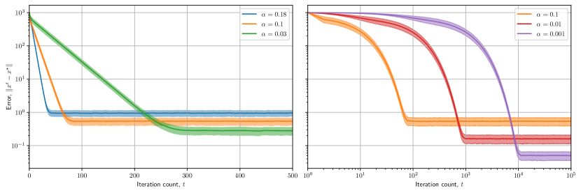
Figure 1: Trade-off between convergence rate and steady-state error (sensitivity to noise). Three different tunings of Gradient Descent (GD) with additive gradient noise are applied to random strongly convex quadratic functions in $\mathbb{R}^{10}$. Half of the Hessian eigenvalues are at $m=1$, the other half at $L=10$. Initialization is $x^{0}=1000\,\mathsf{e}_{1}$. Gradient noise is normally distributed $\mathcal{N}(0,I)$ and i.i.d. across iterations. The plot shows mean and $\pm 1$ standard deviation of the error $\lVert{x^{t}-x^{\star}}\rVert$ for 1000 sample trajectories. Faster convergence comes at the cost of a larger steady-state error, and the trade-off is mediated by the stepsize $\alpha$. On the right panel, iterations are plotted on a log scale to show a larger range of $\alpha$ values.

Gradient Descent is easy to interpret and tune: the choice of stepsize directly mediates the trade-off between convergence rate and sensitivity. Unfortunately, GD is generally slow to converge because it does not exploit the structure present in smooth strongly convex functions, for example. For such functions, alternative methods can provide accelerated convergence rates. Two such methods are Polyak’s Heavy Ball [37] and Nesterov’s Fast Gradient [35], which use the iterations

Heavy Ball (HB): $$\qquad x^{t+1}=x^{t}-\alpha\,g(x^{t})+\beta\,(x^{t}-x^{t-1}),$$ (3)

Fast Gradient (FG): $$\qquad x^{t+1}=x^{t}-\alpha\,g\bigl{(}x^{t}+\beta\,(x^{t}-x^{t-1})\bigr{)}+\beta\,(x^{t}-x^{t-1}).$$ (4)

In the noise-free setting (exact gradient oracle) and under suitable regularity assumptions about the function $f$ such as smoothness and strong convexity, both HB and FG can be tuned in a way that achieves a faster worst-case performance than GD. When using a noisy gradient oracle, these accelerated methods exhibit a stationary phase similar to that of GD in Fig. 1. A trade-off between convergence rate and sensitivity to noise must also exit for HB and FG, but there are now two parameters to tune, so it is unclear how they should be modified to mediate this trade-off.

The goal of this work is to study the trade-off between $\rho$ and $\gamma$ and design practical algorithms that optimize it. We consider three well-studied classes of functions $f:\mathbb{R}^{d}\to\mathbb{R}$ with scalar parameters $m$ and $L$ satisfying $0<m\leq L<\infty$. The function classes are defined as follows.

Smooth strongly convex quadratics ($Q_{m,L}$).

Functions $f(y)=\tfrac{1}{2}(y-y^{\star})^{\mathsf{T}}Q(y-y^{\star})+f^{\star}$ for some $y^{\star}\in\mathbb{R}^{d}$ and $f^{\star}\in\mathbb{R}$, where $Q=Q^{\mathsf{T}}\in\mathbb{R}^{d\times d}$ has eigenvalues in the interval $[m,L]$.

Smooth strongly convex functions ($F_{m,L}$).

Differentiable functions for which $f(y)-\frac{1}{2}m\lVert{y}\rVert^{2}$ is a convex function of $y$ and $\lVert{\nabla\!f(x)-\nabla\!f(y)}\rVert\leq L\lVert{x-y}\rVert$ for all $x,y\in\mathbb{R}^{d}$.

One-point strongly convex functions ($S_{m,L}$).

Differentiable (not necessarily convex) functions for which, for some $y^{\star}\in\mathbb{R}^{d}$, $\bigl{(}\nabla\!f(y)-m(y-y^{\star})\bigr{)}^{\mathsf{T}}\bigl{(}L(y-y^{\star})-\nabla\!f(y)\bigr{)}\geq 0$ for all $y\in\mathbb{R}^{d}$.

These sets of functions are nested in the sense that $Q_{m,L}\subseteq F_{m,L}\subseteq S_{m,L}$, with equality occurring when $m=L$. Moreover, all functions in all of these sets have a unique and arbitrary optimal point, $y^{\star}=\operatorname*{\arg\min}_{y\in\mathbb{R}^{d}}f(y)$. For each function class, we design algorithms of the parameterized form

$$\text{Three-parameter family:}\qquad x^{t+1}=x^{t}-\alpha\,g\bigl{(}x^{t}+\eta\,(x^{t}-x^{t-1})\bigr{)}+\beta\,(x^{t}-x^{t-1}),$$ (5)

where $\alpha$, $\beta$, and $\eta$ are scalar parameters. This algorithm parameterization was first introduced in [26] and is further discussed in Section 2.2. Note that GD, HB, and FG are special cases of the three-parameter family (5) that use $\beta=\eta=0$, $\eta=0$, and $\eta=\beta$, respectively.

1.1 Main contributions

Our three main contributions are as follows.

1. For each function class $Q_{m,L}$, $F_{m,L}$, and $S_{m,L}$, we present a method for efficiently bounding the worst-case convergence rate $\rho$ and sensitivity to additive gradient noise $\gamma$ for a wide class of algorithms. The computational effort required to find the $\rho$ and $\gamma$ bounds for a given algorithm is independent of problem dimension $d$, and takes fractions of a second on a laptop.

2. We present three new algorithms, one for each function class. Each algorithm has the form (5), where $(\alpha,\beta,\eta)$ are explicit algebraic functions of a single tuning parameter that directly trades off convergence rate and sensitivity.

3. We demonstrate through several empirical studies that our algorithm designs closely approximate the Pareto-optimal trade-off between convergence rate and sensitivity to gradient noise. We also show that our algorithm designs compare favorably to (i) popular algorithms such as nonlinear conjugate gradient and quasi-Newton methods, and (ii) existing algorithm designs that use either fewer or more parameters.

Our results can be concisely summarized in Fig. 2, which illustrates the trade-off between convergence rate $\rho$ and noise sensitivity $\gamma$. Our proposed tunable algorithms RHB, RAM, and RGD, are designed for the function classes $Q_{m,L}$, $F_{m,L}$, and $S_{m,L}$, respectively. Each design is a curve in the $(\rho,\gamma)$ space, parameterized by the tuning parameter. Fig. 2 also compares popular algorithms HB, TM, FG, and GD with their recommended tunings (defined in Table 1), which show up as individual points.

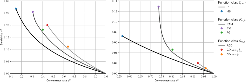
Figure 2: Illustration of the trade-off between steady-state error (sensitivity to noise) $\gamma$, and convergence rate $\rho$ for optimized algorithm designs. Our proposed tunable algorithms RHB, RAM, and RGD are approximately Pareto-optimal for the function classes $Q_{m,L}$, $F_{m,L}$, $S_{m,L}$, respectively. The left panel shows $L=5$ and the right panel shows $L=50$. Both panels use $m=1$, $d=1$, and $\sigma^{2}=1$ (noise variance). Also shown are other algorithms with their recommended tunings, shown as individual colored dots (see Table 1).

Paper organization.

The rest of the paper is organized as follows. In the following subsections, we provide additional background on the problem and describe our analysis and design methodology in more detail. In Section 2, we give a detailed description of the problem setting and performance measures we will be using. Sections 3 to 5 treat the function classes $Q_{m,L}$, $S_{m,L}$, and $F_{m,L}$, respectively. In each of these sections, we develop computationally tractable approaches to computing the convergence rate $\rho$ and noise sensitivity $\gamma$, and we present our optimized algorithm designs. In Section 6, we present empirical studies supporting the near-optimality of our designs and comparing them to existing algorithms. We provide concluding remarks in Section 7.

1.2 Background

There are fundamental lower bounds on the asymptotic convergence rate of iterative methods with noisy gradient oracles. No matter what iterative scheme is used, $\mathbb{E}\lVert{x^{t}-x^{\star}}\rVert^{2}$ cannot decay asymptotically to zero faster than $1/t$. Roughly, this is because the rate at which error can decay is limited by the concentration properties of the gradient noise [34, 1]. This optimal asymptotic rate is achieved by Gradient Descent with a diminishing stepsize that decreases like $1/t$ (henceforth referred to as GDDS). From an asymptotic standpoint, there is no benefit to using anything more complicated than GDDS.

However, GDDS can perform poorly in practice. This is because algorithms are typically run for a predetermined number of iterations (or time budget), or until a predetermined error level is reached. In such settings, it has been shown that transient performance can be dramatically improved through careful manipulation of the stepsize or by using acceleration [23, 19]. One way to exploit the rapid convergence of the transient phase is to use a piecewise constant stepsize, effectively dividing the convergence into epochs where the parameters are held constant within each epoch. This can be done on a predetermined schedule, or by using a statistical test to detect the phase transition which then triggers the parameter change [9]. When the gradient noise is due to sampling a finite-sum objective function, other strategies include incremental gradient (or variance reduction) methods [24, 11]. Specific algorithms have also been studied in the stochastic case, such as Stochastic Gradient Descent [32] and the Multi-Stage Accelerated Stochastic Gradient method [4] that resets the momentum periodically.

While we restrict our attention to additive stochastic gradient noise, other inexact oracles have been studied. The most prominent alternative model is to assume deterministic bounded noise, which may be additive or multiplicative. In [15], the authors show that under an additive deterministic oracle, acceleration necessarily results in an accumulation of gradient errors. In [22], the authors analyze Stochastic Gradient Descent under a hybrid additive and multiplicative deterministic oracle. In [26], the authors study a multiplicative deterministic oracle and in [10], the authors develop the Robust Momentum (RM) to trade off convergence rate and sensitivity for this oracle. In his thesis, Devolder studies both stochastic and deterministic oracles in the weakly convex case [12]. With others, he also studies deterministic oracles in the strongly convex case [13] and constructs intermediate gradient methods to exploit the trade-off between convergence rate and sensitivity to gradient noise in the deterministic and weakly convex case [14].

1.3 Methodology

We now provide an overview of our analysis and design framework and point to related techniques. Our method for bounding the convergence rate $\rho$ and sensitivity $\gamma$ for the classes $S_{m,L}$ and $F_{m,L}$ relies on solving a small linear matrix inequality (LMI). This idea builds upon several related works.

• The performance estimation framework [16, 40] uses LMIs to directly search for a trajectory achieving the worst-case performance over a finite number of iterations. This approach provides an exact characterization of the performance, although the dimension of the LMI grows with the length of the trajectory.

• Viewing algorithms as discrete-time dynamical systems, Integral Quadratic Constraints from control theory [26, 29, 18] may be used to search for worst-case performance guarantees. This approach also leads to LMIs and characterizes the asymptotic performance of an algorithm, although the ensuing performance bounds may not be tight in general.

• Finally, LMIs may be used to directly search for a Lyapunov function, which is a generalized notion of “energy” stored in the system. If a fraction of the energy dissipates at each iteration, this is akin to proving convergence at a specified rate [21, 39]. Similar to IQCs, Lyapunov functions provide asymptotic (albeit more interpretable) performance guarantees.

In the present work, we adopt a Lyapunov approach most similar to [39], but we generalize it to include both convergence rate and sensitivity to noise. We also explain in Section 5.3 how the three aforementioned approaches are connected to one another. Given an LMI that establishes the performance (convergence rate or sensitivity to noise) of a given first-order method, the next step is to design algorithms that exploit this trade-off. Several approaches have been proposed.

• One can parameterize a family of candidate algorithms, and search over algorithm parameters to achieve an optimal trade-off between convergence rate $\rho$ and sensitivity $\gamma$ to gradient noise. For example, for every fixed $\rho$, one could seek algorithm parameters that achieve the minimum possible $\gamma$. Such a problem is typically non-convex, so one must resort to exhaustive search [26] or nonlinear numerical solvers that find local optima.

• Using convex relaxations or other heuristics such as coordinate descent, the algorithm design problem can be solved approximately. While this approach may lead to conservative designs, it has the benefit of being automated, flexible, and amenable to efficient convex solvers [29].

• In certain settings, the controller parameters can be eliminated from the LMI entirely, yielding bounds that hold for all algorithms. This approach has been used to show that the Triple Momentum (TM) method achieves the optimal worst-case rate over the class $F_{m,L}$ [27, 38].

As in the above approaches, we parameterize a family of candidate algorithms via (5). However, our approach to algorithm design is algebraic rather than numeric. We find analytic solutions to the non-convex semidefinite programs that arise when the algorithm parameters are treated as decision variables. This approach enables us to find explicit analytic expressions for our algorithm parameters rather than having to specify them implicitly. Nevertheless, we still make use of numerical approaches in order to validate our choice of parameterization and the near-optimality of our designs, and to compare the performance of our designs to that of existing algorithms; see Section 6. Our design procedure is outlined as follows.

1. Choose the function class. For each algorithm design, we choose one of the function classes $Q_{m,L}$, $F_{m,L}$, or $S_{m,L}$. We typically choose $L/m=10$ or $100$, since larger ratios of $L/m$ may cause the analysis to be ill-conditioned while smaller ratios are typically irrelevant and may lead to different expressions for the stepsizes of the designed algorithm.

2. Numerically find a near-Pareto-optimal algorithm. As described previously, searching directly over algorithm parameters is often a non-convex problem. However, a near-Pareto-optimal solution may be found using exhaustive search or a nonlinear numerical solver.

3. Find the active constraints. Use the numerical values of the near-Pareto-optimal algorithm to determine the active constraints. For analyses based on LMIs, the associated matrices will drop rank at the optimal solution, giving rise to a set of equations. In particular, if a matrix has rank $r$, then all of its $(r+1)\times(r+1)$ minors are zero.

4. Solve the set of equations. Now, we can solve the active constraint equations to obtain algebraic expressions for the algorithm parameters. For analyses based on LMIs, the set of active constraints is a system of polynomial equations. One way to solve such a system is to compute a Gröbner basis, which provides a means of characterizing all solutions to a set of polynomial equations, similar to Gaussian elimination for linear systems. While many software implementations exist to compute such a basis, these algorithms are typically inefficient for the large system of equations produced by the LMIs. Instead of describing all solutions, we instead use Mathematica [43] to search for the single solution that describes the numerical near-Pareto-optimal algorithm and its corresponding solution to the LMI obtained previously. Some heuristics that we used were:

   • first eliminate variables that appear linearly, since the resulting system after back-substitution remains a polynomial,

   • observe whether any equations factor, in which case we can use the numerical solution to determine which factor to set to zero.

Our design process results in algebraic expressions for the algorithm parameters and any other variables used in the analysis (such as the solution to an LMI). In some cases, our designed algorithm has simple expressions for the stepsizes and achieves the Pareto-optimal trade-off between convergence rate and sensitivity, such as our Robust Heavy Ball method for the function class $Q_{m,L}$. The other function classes $S_{m,L}$ and $F_{m,L}$, however, do not seem to admit Pareto-optimal algorithms with such a simple form. The challenge is then to find suboptimal algorithms that are near-Pareto-optimal for relevant ranges of $L$ and $m$ values and also have simple algebraic expressions for the parameters.

2 Problem setting and assumptions

To solve the optimization problem (1), we consider iterative first-order methods described by linear time-invariant dynamics of the form

$$\xi^{t+1} =A\xi^{t}+B(u^{t}+w^{t}),$$ (6a)

$$y^{t} =C\xi^{t},$$ (6b)

$$u^{t} =\nabla\!f(y^{t}),$$ (6c)

where $\xi^{t}\in\mathbb{R}^{n\times d}$ is the state of the algorithm, $y^{t}\in\mathbb{R}^{1\times d}$ is the point at which the gradient is evaluated, $u^{t}\in\mathbb{R}^{1\times d}$ is the (exact) value of the gradient, $w^{t}\in\mathbb{R}^{1\times d}$ is the gradient noise, and $t$ is the iteration. The state is the memory of the algorithm because its size reflects the number of past iterates that must be stored at each timestep. Solutions of the dynamical system are called trajectories. For example, given an algorithm $(A,B,C)$, particular function $f$, initial condition $\xi^{0}$, and noise distribution $w\sim\mathbb{P}$, a trajectory is any sequence $(\xi^{t},u^{t},y^{t},w^{t})_{t\geq 0}$ that satisfies (6). This framework is very general and encompasses a wide variety of fixed-parameter first-order iterative methods; we discuss this in more detail in Section 2.2.

Remark 1 (important notational convention).

Throughout the paper, we represent iterates as row vectors, so that the matrices $A\in\mathbb{R}^{n\times n}$, $B\in\mathbb{R}^{n\times 1}$, and $C\in\mathbb{R}^{1\times n}$ act on the columns of the iterates while the gradient oracle $\nabla\!f:\mathbb{R}^{1\times d}\to\mathbb{R}^{1\times d}$ acts on the rows. Because of this convention, $\lVert{\cdot}\rVert$ denotes the Frobenius norm, for example, $\lVert{\xi^{t}}\rVert^{2}\mathrel{\mathchoice{\vbox{\hbox{$\displaystyle:$}}}{\vbox{\hbox{$\textstyle:$}}}{\vbox{\hbox{$\scriptstyle:$}}}{\vbox{\hbox{$\scriptscriptstyle:$}}}{=}}\sum_{i=1}^{n}\sum_{j=1}^{d}(\xi^{t}_{ij})^{2}$. This framework decouples the state dimension of the algorithm ($n$) from the dimension of the objective function’s domain ($d$).

In our model (6), the noise corrupts the gradient $u^{t}$, although it is straightforward to modify our analysis to other scenarios, such as when the noise corrupts the entire state $\xi^{t}$.

For each of the function classes considered, the objective function $f$ has a unique optimizer $y^{\star}$. We also make the following assumption regarding the algorithm (6).

Assumption 2 (deterministic fixed point).

For any $y^{\star}$ such that $\nabla\!f(y^{\star})=0$, there exists $\xi^{\star}$ such that $\xi^{\star}=A\xi^{\star}$ and $y^{\star}=C\xi^{\star}$.

The fixed point assumption is a necessary condition for convergence to the optimal point because it ensures that if we initialize our algorithm at $\xi^{0}=\xi^{\star}$ and there is no gradient noise, subsequent iterates will remain at $\xi^{\star}$. Since we are doing worst-case analysis, we may assume without loss of generality that the optimal point is at the origin. We formalize this fact in the following lemma.

Lemma 3 (fixed point shifting).

Let $\mathcal{F}\in\{Q_{m,L},F_{m,L},S_{m,L}\}$ be one of the function classes defined in Section 1. Consider a function $f\in\mathcal{F}$ with optimal point $y^{\star}$, optimal function value $f^{\star}\mathrel{\mathchoice{\vbox{\hbox{$\displaystyle:$}}}{\vbox{\hbox{$\textstyle:$}}}{\vbox{\hbox{$\scriptstyle:$}}}{\vbox{\hbox{$\scriptscriptstyle:$}}}{=}}f(y^{\star})$, and optimal gradient $u^{\star}=0$. Then the function $\tilde{f}:y\mapsto f(y+y^{\star})-f^{\star}$ has the property that $\tilde{f}\in\mathcal{F}$ with optimal point, optimal function value, and optimal gradient all zero.

Let $(A,B,C)$ be an algorithm of the form (6) satisfying 2. Define the shifted coordinates $\tilde{\xi}^{t}\mathrel{\mathchoice{\vbox{\hbox{$\displaystyle:$}}}{\vbox{\hbox{$\textstyle:$}}}{\vbox{\hbox{$\scriptstyle:$}}}{\vbox{\hbox{$\scriptscriptstyle:$}}}{=}}\xi^{t}-\xi^{\star}$ and similarly for $\tilde{y}^{t}$ and $\tilde{u}^{t}$. Then we may rewrite (6) in shifted coordinates as:

$$\tilde{\xi}^{t+1} =A\tilde{\xi}^{t}+B(\tilde{u}^{t}+w^{t})$$ (7a)

$$\tilde{y}^{t} =C\tilde{\xi}^{t}$$ (7b)

$$\tilde{u}^{t} =\nabla\!\tilde{f}(\tilde{y}^{t})$$ (7c)

In other words, we may assume without loss of generality that $y^{\star}=0$ and $f^{\star}=f(y^{\star})=0$.

In the remainder of this section, we provide definitions of the convergence rate $\rho$ and noise sensitivity $\gamma$ introduced in Section 1, and we parameterize the set of algorithms considered for design.

2.1 Performance evaluation

As alluded to in Section 1, we consider the trade-off between convergence rate and sensitivity to additive stochastic gradient noise. Let $\mathcal{A}=(A,B,C)$ denote an algorithm as defined in (6) and let $\mathcal{F}\in\{Q_{m,L},F_{m,L},S_{m,L}\}$ denote one of the families of functions defined in Section 1.

Convergence rate.

The convergence rate $\rho$ describes the first phase of convergence observed in Fig. 1: exponential decrease of the error. In this regime, gradients are relatively large compared to the noise, so we assume $w^{t}=0$ for all $t\geq 0$. For any algorithm $\mathcal{A}$ with initial point $\xi^{0}$ and fixed point $\xi^{\star}$ and any function $f\in\mathcal{F}$, consider the trajectory $(\xi^{0},\xi^{1},\dots)$ produced by $\mathcal{A}$. We define the convergence rate to be:

$$\rho(\mathcal{A},\mathcal{F})\mathrel{\mathchoice{\vbox{\hbox{$\displaystyle:$}}}{\vbox{\hbox{$\textstyle:$}}}{\vbox{\hbox{$\scriptstyle:$}}}{\vbox{\hbox{$\scriptscriptstyle:$}}}{=}}\inf\left\{\rho>0\;|\;\sup_{f\in\mathcal{F}}\,\sup_{\xi^{0}\in\mathbb{R}^{n\times d}}\,\sup_{t\geq 0}\,\frac{\lVert{\xi^{t}-\xi^{\star}}\rVert}{\rho^{t}\lVert{\xi^{0}-\xi^{\star}}\rVert}<\infty\right\}.$$ (8)

In other words, if the convergence rate $\rho_{0}=\rho(\mathcal{A},\mathcal{F})$ is finite, then for all $\varepsilon>0$, there exists a constant $c$ such that the trajectory satisfies the bound $\lVert{\xi^{t}-\xi^{\star}}\rVert\leq c\,(\rho_{0}+\varepsilon)^{t}\lVert{\xi^{0}-\xi^{\star}}\rVert$ for all functions $f\in\mathcal{F}$, initial points $\xi^{0}\in\mathbb{R}^{n\times d}$, and iterations $t\geq 0$. This definition of $\rho$ corresponds to the conventional notion of linear convergence rate used in the worst-case analysis of deterministic algorithms. If $\rho_{0}<1$, the algorithm is said to be globally linearly convergent, and for all $\varepsilon>0$, we have $\lVert{\xi^{t}-\xi^{\star}}\rVert=O((\rho_{0}+\varepsilon)^{t})$ and $\lVert{y^{t}-y^{\star}}\rVert=O((\rho_{0}+\varepsilon)^{t})$. A smaller value of $\rho_{0}$ corresponds to a faster (worst-case) convergence rate.

While we characterize convergence of the algorithm using the convergence rate $\rho$, the optimization and machine learning literature typtically uses the iteration complexity, which is the number of iterations required for the algorithm to achieve an error below some threshold. While these quantities are related, the convergence rate provides a more fine-tuned characterization of the convergence. For instance, while the iteration complexity of Nesterov’s FG method is optimal for the function class $F_{m,L}$, the convergence rate is strictly suboptimal [42].

Sensitivity.

The sensitivity $\gamma$ characterizes the steady-state phase of convergence observed in Fig. 1. The steady-state error depends on the noise characteristics. We will assume that the noise sequence $w^{0},w^{1},\dots$ has joint distribution $\mathbb{P}\in\mathcal{P}_{\sigma}$, with parameter $\sigma$ to be defined shortly. We assume the set of admissible joint distributions $\mathcal{P}_{\sigma}$ satisfies:

1. Independence across time. For all $\mathbb{P}\in\mathcal{P}_{\sigma}$, if $w\sim\mathbb{P}$, then $w^{t}$ and $w^{\tau}$ are independent for all $t\neq\tau$. Then we may characterize the joint distribution $\mathbb{P}\in\mathcal{P}_{\sigma}$ by its associated marginal distributions $(\mathbb{P}^{0},\mathbb{P}^{1},\dots)$. We do not assume the $\mathbb{P}^{t}$ are necessarily identical.

2. Zero-mean and bounded covariance. For all $(\mathbb{P}^{0},\mathbb{P}^{1},\dots)\in\mathcal{P}_{\sigma}$, we have $\operatorname{\mathbb{E}}_{w^{t}\sim\mathbb{P}^{t}}(w^{t})=0$ and $\operatorname{\mathbb{E}}_{w^{t}\sim\mathbb{P}^{t}}({w^{t}}^{\mathsf{T}}w^{t})\preceq\sigma^{2}I_{d}$. We assume $\sigma$ is known for the purpose of our analysis.

Our assumptions on the noise imply that $\mathcal{P}_{\sigma}$ is completely characterized by the variance bound $\sigma^{2}$. For any fixed algorithm $\mathcal{A}$, function $f\in\mathcal{F}$, initial point $\xi^{0}$, and family of noise distributions $\mathcal{P}_{\sigma}$, consider the stochastic iterate sequence $y^{0},y^{1},\dots$ produced by $\mathcal{A}$ and let $y^{\star}\mathrel{\mathchoice{\vbox{\hbox{$\displaystyle:$}}}{\vbox{\hbox{$\textstyle:$}}}{\vbox{\hbox{$\scriptstyle:$}}}{\vbox{\hbox{$\scriptscriptstyle:$}}}{=}}\operatorname*{\arg\min}_{y\in\mathbb{R}^{d}}f(y)$ be the unique minimizer of $f$. We define the noise sensitivity to be:

$$\gamma(\mathcal{A},\mathcal{F},\sigma^{2})=\sup_{f\in\mathcal{F}}\,\sup_{\xi^{0}\in\mathbb{R}^{n\times d}}\,\sup_{\mathbb{P}\in\mathcal{P}_{\sigma}}\,\,\limsup_{T\to\infty}\sqrt{\operatorname{\mathbb{E}}_{w\sim\mathbb{P}}\,\frac{1}{T}\sum_{t=0}^{T-1}\bigl{\lVert}{y^{t}-y^{\star}}\bigr{\rVert}^{2}}.$$ (9)

A smaller value of $\gamma$ is desirable because it means the algorithm achieves small error in spite of gradient perturbations. This definition for $\gamma$ is similar to that used in recent works exploring first-order algorithms with additive gradient noise using a robust $\mathcal{H}_{2}$ approach [31, 5, 29].

Remark 4 (bounded sensitivity).

If $\rho(\mathcal{A},\mathcal{F})<1$, then $\gamma(\mathcal{A},\mathcal{F},\sigma^{2})<\infty$ for any $\sigma$. This is a consequence of 11, which establishes the fact for $S_{m,L}$, the largest of the function families. The converse need not hold. For example, if $A$ is chosen such that $\rho(A)>1$, then picking $C=0$ yields $\gamma(\mathcal{A},\mathcal{F},\sigma^{2})=\lVert{y^{\star}}\rVert<\infty$, and picking $B=0$ yields $\rho(\mathcal{A},\mathcal{F})=\rho(A)>1$.

Remark 5.

Some authors [29, 31] compute the sensitivity with respect to the squared-norm of the state $\|\xi^{t}-\xi^{\star}\|^{2}$. This quantity, however, depends on the state-space realization; performing a similarity transformation $(A,B,C)\mapsto(TAT^{-1},TB,CT^{-1})$ for some invertible matrix $T$ does not change the input $u^{t}$ or output $y^{t}$ of the system, but it does map the state as $\xi^{t}\mapsto T\xi^{t}$ and therefore scales the sensitivity when measured with respect to the state. Instead, we compute the sensitivity with respect to the squared-norm of the output $\|y^{t}-y^{\star}\|^{2}$, which is invariant under similarity transformations. It is straightforward to modify our analysis to compute the sensitivity with respect to other quantities, such as the squared-norm of the gradient $\|u^{t}\|^{2}$ or the function values $f(y^{t})-f^{\star}$.

2.2 Algorithm parameterization

While our analysis applies to the general algorithm model (6), for the purpose of design we will further restrict the class of algorithms to those with state dimension $n=2$. At first, it may appear that algorithms of the form (6) have $n^{2}+2n$ degrees of freedom since we are free to choose $A,B,C$ however we like, so describing the case $n=2$ should require $8$ parameters. However, many of these parameters are redundant, and if we further assume the fixed point condition of 2, the case $n=2$ can be fully parameterized using only three scalar parameters $(\alpha,\beta,\eta)$ as follows:

$$\xi^{t} \mathrel{\mathchoice{\vbox{\hbox{$\displaystyle:$}}}{\vbox{\hbox{$\textstyle:$}}}{\vbox{\hbox{$\scriptstyle:$}}}{\vbox{\hbox{$\scriptscriptstyle:$}}}{=}}\begin{bmatrix}x^{t}\\ x^{t-1}\end{bmatrix}, A =\begin{bmatrix}1+\beta&-\beta\\ 1&0\end{bmatrix}, B =\begin{bmatrix}-\alpha\\ 0\end{bmatrix}, C =\begin{bmatrix}1+\eta&-\eta\end{bmatrix},$$ (10)

which is equivalent to our three-parameter family (5). We will refer to specific algorithms from this family by their triplet of parameters $(\alpha,\beta,\eta)$. Later in Section 6.3, we provide numerical evidence that further justifies our choice of parameterization.

To see that three parameters are sufficient to capture all algorithms with $n=2$ states, consider the transfer function of the algorithm [2, §2.7], which is the linear map from the $z$-transform of $w^{t}$ to the $z$-transform of $y^{t}$ given by the rational function: $G(z)=C(zI-A)^{-1}B$. When $n=2$, $G(z)$ is a rational function with numerator degree at most $1$ and denominator degree at most $2$. The poles of $G(z)$ correspond to the eigenvalues of $A$, and by 2, one of those eigenvalues is fixed at $1$. This leaves three degrees of freedom. In particular, the transfer function for (10) is:

$$G(z)=-\alpha\,\frac{(1+\eta)z-\eta}{(z-1)(z-\beta)}.$$

The redundancy in the $(A,B,C)$ parameterization stems from the fact that given any invertible matrix $T\in\mathbb{R}^{n\times n}$, algorithms $(A,B,C)$ and $(TAT^{-1},TB,CT^{-1})$ have the same transfer function. Moreover, if we initialize these algorithms with initial state $\xi^{0}$ and $T\xi^{0}$ respectively, they will have the same trajectories $(y^{0},y^{1},\dots)$. Therefore, both algorithms share the same performance metrics $\rho$ and $\gamma$. Such transformations are called state-space similarity transformations [45, §3.3].

By choosing specific values for $(\alpha,\beta,\eta)$, the algorithm (5) recovers several known algorithms. We describe these algorithms in Table 1, as they will serve as useful benchmarks for our designs.

Table 1: Comparison of different algorithms, their recommended/standard tunings, and applicable function classes. For RM, the tuning parameter satisfies $1-\sqrt{\frac{m}{L}}\leq\rho\leq 1-\frac{m}{L}$. When $\rho=1-\sqrt{\frac{m}{L}}$, RM becomes TM; when $\rho=1-\frac{m}{L}$, RM becomes GD with $\alpha=\frac{1}{L}$.

Algorithm name	$\alpha$	$\beta$	$\eta$	Func. class
Gradient Descent (GD)	$\frac{1}{L}$ or $\frac{2}{L+m}$	0	0	$S_{m,L}$
Heavy Ball (HB), [37]	$\frac{4}{(\sqrt{L}+\sqrt{m})^{2}}$	$\left(\frac{\sqrt{L}-\sqrt{m}}{\sqrt{L}+\sqrt{m}}\right)^{2}$	0	$Q_{m,L}$
Fast Gradient (FG), [35]	$\frac{1}{L}$	$\frac{\sqrt{L}-\sqrt{m}}{\sqrt{L}+\sqrt{m}}$	$\frac{\sqrt{L}-\sqrt{m}}{\sqrt{L}+\sqrt{m}}$	$F_{m,L}$
Triple Momentum (TM), [42]	$\frac{\sqrt{L}-\sqrt{m}}{L^{3/2}}$	$\frac{(\sqrt{L}-\sqrt{m})^{2}}{L+\sqrt{mL}}$	$\frac{(\sqrt{L}-\sqrt{m})^{2}}{2L-m+\sqrt{mL}}$	$F_{m,L}$
Robust Momentum (RM), [10]	$\frac{(1-\rho)^{2}(1+\rho)}{m}$	$\frac{L\rho^{3}}{L-m}$	$\frac{m\rho^{3}}{(L-m)(1-\rho)^{2}(1+\rho)}$	$F_{m,L}$

Different triples $(\alpha,\beta,\eta)$ generally correspond to different algorithms, with one important exception: Gradient Descent has a degenerate family of possible parameterizations.

Proposition 6.

Gradient Descent with parameterization $(\alpha,0,0)$ can also be parameterized by $\bigl{(}\alpha(1-\beta),\beta,\frac{\beta}{1-\beta}\bigr{)}$ for any choice of $\beta\neq 1$.

6 follows from the fact that when we substitute $(\alpha,\beta,\eta)\mapsto\bigl{(}\alpha(1-\beta),\beta,\frac{\beta}{1-\beta}\bigr{)}$ into (5), the update equation can be rearranged to obtain

$$\left(\frac{x^{t+1}-\beta x^{t}}{1-\beta}\right)=\left(\frac{x^{t}-\beta x^{t-1}}{1-\beta}\right)-\alpha\,\nabla\!f\left(\frac{x^{t}-\beta x^{t-1}}{1-\beta}\right)-\alpha w^{t}.$$ (11)

In other words, it is simply Gradient Descent applied to the quantity $y^{t}\mathrel{\mathchoice{\vbox{\hbox{$\displaystyle:$}}}{\vbox{\hbox{$\textstyle:$}}}{\vbox{\hbox{$\scriptstyle:$}}}{\vbox{\hbox{$\scriptscriptstyle:$}}}{=}}\frac{1}{1-\beta}(x_{t}-\beta x_{t-1})$. The equivalence can also be seen by observing that the transfer function $G(z)$ simplifies to $G(z)=\frac{-\alpha}{z-1}$ due to a pole-zero cancellation of the factor $(z-\beta)$, so we recover the transfer function of GD.

In the next three sections, we focus on the function classes $Q_{m,L}$, $S_{m,L}$, and $F_{m,L}$, respectively. For each class, we provide a tractable approach for computing the performance metrics $\rho$ and $\gamma$, and we design algorithms of the form (5) that provide a near-optimal trade-off between $\rho$ and $\gamma$.

3 Smooth strongly convex quadratic functions

We begin with the class $Q_{m,L}$ of strongly convex quadratics. We will first derive exact formulas for the worst-case convergence rate and the sensitivity to additive gradient noise.

3.1 Performance bounds for $Q_{m,L}$

The quadratic case has been treated extensively in recent works on algorithm analysis [26, 5, 31]. We now present versions of these results adapted to our algorithm class of interest. When $f$ is a positive definite quadratic and we shift the fixed-point to zero using 2, we can write $\nabla\!f(y)=yQ$ for some $Q\in\mathbb{R}^{d\times d}$ satisfying $Q=Q^{\mathsf{T}}\succ 0$ (recall that the iterates are row vectors, so $y\in\mathbb{R}^{1\times d}$). The algorithm’s dynamics (7) become

$$\xi^{t+1}=A\xi^{t+1}+BC\xi^{t}Q+Bw^{t}\quad\text{and}\quad y^{t}=C\xi^{t}.$$ (12)

If we diagonalize $Q$, we can split the dynamics into $d$ decoupled systems, each of the form:

$$\hat{\xi}^{t+1} =(A+qBC)\hat{\xi}^{t}+B\hat{w}^{t}$$ (13a)

$$\hat{y}^{t} =C\hat{\xi}^{t},$$ (13b)

where $q$ is an eigenvalue of $Q$, and we now have $\hat{\xi}^{t}\in\mathbb{R}^{n\times 1}$, $\hat{y}^{t}\in\mathbb{R}$, and $\hat{w}^{t}\in\mathbb{R}$. The performance metrics $\rho$ and $\gamma$ of the original system can be obtained by analyzing the simpler system (13). In particular, the convergence rate $\rho$ is the spectral radius of the system matrix $A+qBC$. With regards to the sensitivity $\gamma$, we observe that since the covariance of $w^{t}$ was bounded by $\sigma^{2}I_{d}$, the covariance of $\hat{w}^{t}$ is bounded by $\sigma^{2}$. Due to the way $\gamma$ is defined in (9), we can compute $\gamma^{2}$ separately for each decoupled system (13) and sum them together to obtain $\gamma^{2}$ for the original system. We summarize the results in the following proposition.

Proposition 7 ($Q_{m,L}$ analysis, general).

Consider an algorithm $\mathcal{A}=(A,B,C)$ defined in (6) satisfying 2 applied to a strongly convex quadratic $f\in Q_{m,L}$ defined in Section 1 with additive gradient noise with covariance bound $\sigma^{2}I_{d}$. The algorithm has convergence rate

$$\rho(\mathcal{A},Q_{m,L})=\sup_{q\in[m,L]}\rho\bigl{(}A+qBC\bigr{)}.$$

If $\rho(\mathcal{A},Q_{m,L})<1$, the algorithm has sensitivity

$$\gamma(\mathcal{A},Q_{m,L},\sigma^{2})=\sup_{q\in[m,L]}\sqrt{\sigma^{2}d\cdot(B^{\mathsf{T}}P_{q}B)},$$

where $P_{q}$ is the solution to the linear equation $(A+qBC)^{\mathsf{T}}P_{q}(A+qBC)-P_{q}+C^{\mathsf{T}}C=0$.

Here, $\rho(\cdot)$ denotes the spectral radius (largest eigenvalue magnitude). Results similar to 7 have appeared in the context of algorithm analysis for quadratic functions in [5, 31], and make use of the fact that the sensitivity $\gamma$ is equivalent to the $\mathcal{H}_{2}$ norm, which can be computed using a Lyapunov approach.

The expressions in 7 may be difficult to evaluate if the matrices $(A,B,C)$ are large. Fortunately, the sizes of these matrices only depend on the state dimension $n$, which is typically small ($n\leq 2$ for all methods in Table 1). The dimension $d$ of the function domain does not appear in the expression for $\rho$, and only appears as a proportionality constant in the expression for $\gamma$.

3.2 Algorithm design for $Q_{m,L}$

For strongly convex quadratic functions, first-order methods can achieve exact convergence in $d$ iterations, where $d$ is the dimension of the domain of $f$. One such example is the Conjugate Gradient (CG) method [36, Thm. 5.4]. However, when the number of iterations $t$ satisfies $t<d$, exact convergence is not possible in general. Nesterov’s lower bound [35, Thm. 2.1.13] demonstrates that for any $t\geq 0$, one can construct a function $f\in Q_{m,L}$ with domain dimension $d>t$ such that:

$$\lVert{y^{t}-y^{\star}}\rVert\geq\left(\frac{\sqrt{L}-\sqrt{m}}{\sqrt{L}+\sqrt{m}}\right)^{t}\lVert{y^{0}-y^{\star}}\rVert.$$ (14)

This lower bound holds for any first-order method such that $y^{t}$ is a linear combination of $y^{0}$ and past gradients $\nabla\!f(y^{0}),\dots,\nabla\!f(y^{t-1})$. This class includes not only CG but also methods with unbounded memory.

In the regime $t<d$, the CG method matches Nesterov’s lower bound [36, Thm. 5.5] and is therefore optimal in terms of worst-case rate. However, it is not is not clear how CG should be adjusted to be robust in the presence of additive gradient noise, since it has no tunable parameters.

The Heavy Ball method (3), when tuned as in Table 1, also matches Nesterov’s lower bound when applied to the function class $Q_{m,L}$ [37, §3.2.1], but has a simpler implementation than CG: its updates are linear and its parameters are constant.

We adopted the three-parameter class $(\alpha,\beta,\eta)$ described in Section 2.2 as our search space for optimized algorithms because the Heavy Ball method is a special case of this family and Heavy Ball can achieve optimal performance on $Q_{m,L}$ when there is no noise. Substituting the three-parameter algorithm (10) into 7, we obtain the following result.

Corollary 8 ($Q_{m,L}$ analysis, reduced).

Consider the three-parameter algorithm $\mathcal{A}=(\alpha,\beta,\eta)$ defined in Section 2.2. For the function class of strongly convex quadratics $Q_{m,L}$ with noise covariance bound $\sigma^{2}I_{d}$, we have

$$\rho(\mathcal{A},Q_{m,L}) =\max_{q\in\{m,L\}}\begin{cases}\sqrt{\beta-\alpha\eta q}&\text{if }\Delta<0\\ \frac{1}{2}\left(|\beta+1-\alpha q-\alpha\eta q|+\sqrt{\Delta}\right)&\text{if }\Delta\geq 0\end{cases}$$ (15)

$$\quad\text{where }\Delta\mathrel{\mathchoice{\vbox{\hbox{$\displaystyle:$}}}{\vbox{\hbox{$\textstyle:$}}}{\vbox{\hbox{$\scriptstyle:$}}}{\vbox{\hbox{$\scriptscriptstyle:$}}}{=}}(\beta+1-\alpha q-\alpha\eta q)^{2}-4(\beta-\alpha\eta q).$$

If $\rho(\mathcal{A},Q_{m,L})<1$, we also have

$$\gamma(\mathcal{A},Q_{m,L},\sigma^{2})=\max_{q\in\{m,L\}}\sqrt{\frac{\sigma^{2}d\,\alpha(1+\beta+(1+2\eta)\alpha\eta q)}{q(1-\beta+\alpha\eta q)(2+2\beta-(1+2\eta)\alpha q)}}.$$ (16)

In 8, the suprema from 7 are replaced by a simple maximum; we only need to check the endpoints of the interval $[m,L]$ because both $\rho$ and $\gamma$ are quasiconvex functions of $q$ when $n\leq 2$. See Section A.1 for a proof.

Our proposed algorithm for the class $Q_{m,L}$ is a special tuning of Heavy Ball, which we named Robust Heavy Ball (RHB). The RHB algorithm was found by careful analysis of the analytic expressions for $\rho$ and $\gamma$ in 8. The algorithm is described in the following theorem, which we prove in Section A.2.

Theorem 9 (Robust Heavy Ball, RHB).

Consider the function class $Q_{m,L}$ and let $\rho$ be a parameter chosen with $\frac{\sqrt{L}-\sqrt{m}}{\sqrt{L}+\sqrt{m}}\leq\rho<1$. Then, the algorithm $\mathcal{A}$ of the form (5) with noise covariance bound $\sigma^{2}I_{d}$ and tuning $\alpha=\frac{1}{m}(1-\rho)^{2}$, $\beta=\rho^{2}$, and $\eta=0$ achieves the performance metrics

$$\rho(\mathcal{A},Q_{m,L})=\rho,\qquad\gamma(\mathcal{A},Q_{m,L},\sigma^{2})=\frac{\sigma\sqrt{d}}{m}\sqrt{\frac{1-\rho^{4}}{(1+\rho)^{4}}}.$$

Although we set out to design an algorithm in the three-parameter class $(\alpha,\beta,\eta)$, it turns out that Pareto-optimal algorithms can be found with $\eta=0$ (Heavy Ball). In other words, it is unnecessary to use a nonzero $\eta$ when optimizing over the class $Q_{m,L}$.

If we choose the smallest possible $\rho=\frac{\sqrt{L}-\sqrt{m}}{\sqrt{L}+\sqrt{m}}$ (fastest possible convergence rate), then we recover Polyak’s tuning of HB, whose convergence rate matches Nesterov’s lower bound. It is straightforward to check that $\gamma$ is a monotonically decreasing function of $\rho$, so as the convergence rate slows down ($\rho$ increases), the algorithm becomes less sensitivity to noise ($\gamma$ decreases).

4 One-point strongly convex functions

We now consider the class $S_{m,L}$ of functions satisfying the one-point strong convexity condition:

$$\bigl{(}\nabla\!f(y)-m\,(y-y^{\star})\bigr{)}^{\mathsf{T}}\bigl{(}L\,(y-y^{\star})-\nabla\!f(y)\bigr{)}\geq 0\qquad\text{for all }y\in\mathbb{R}^{d}.$$

If we view $y$ and $\nabla\!f(y)$ as row vectors instead, this condition can be conveniently rewritten as the trace of a quadratic form:

$$\operatorname{\mathrm{tr}}\begin{bmatrix}y-y^{\star}\\ \nabla\!f(y)\end{bmatrix}^{\mathsf{T}}\begin{bmatrix}-2mL&m+L\\ m+L&-2\end{bmatrix}\begin{bmatrix}y-y^{\star}\\ \nabla\!f(y)\end{bmatrix}\geq 0\qquad\text{for all }y\in\mathbb{R}^{1\times d}.$$ (17)

Functions $f\in S_{m,L}$ are not necessarily convex, yet first-order methods can still achieve linear convergence rates over this function class [33].

4.1 Performance bounds for $S_{m,L}$

The set $S_{m,L}$ is much larger than $Q_{m,L}$ and not readily parameterizable, so we adopt the approach of looking for a Lyapunov function to certify convergence and robustness properties.

To certify convergence, we adopt the approach used in [26] for so-called pointwise constraints. The goal is to find a Lyapunov function, which is a function $V:\mathbb{R}^{n}\to\mathbb{R}$ that satisfies the following conditions for all trajectories of the noise-free ($\sigma=0$) algorithm:

• Lower bound condition: $V(\xi^{t})\geq\lVert{\xi^{t}-\xi^{\star}}\rVert^{2}$

• Decrease condition: $V(\xi^{t+1})\leq\rho^{2}V(\xi^{t})$ for some fixed $\rho>0$

These conditions imply that $\lVert{\xi^{t}-\xi^{\star}}\rVert^{2}\leq V(\xi^{t})\leq\rho^{2t}V(\xi^{0})$ and therefore provide a way to certify convergence with a given rate $\rho$. Assuming $V$ is a positive semidefinite quadratic function allows the search for a Lyapunov function to be cast as a semidefinite program and solved efficiently.

To certify robustness, we adopt the approach from [31, Lem. 1]. A more general version of this approach was developed in [29] and a similar approach is used in [5] to obtain performance bounds that combine both $\rho$ and $\gamma$ into a single bound. The goal is again seek a function $V:\mathbb{R}^{n}\to\mathbb{R}$, but with slightly different conditions. For all trajectories of the algorithm, we require:

• Lower bound condition: $\operatorname{\mathbb{E}}V(\xi^{t})\geq 0$

• Increment condition: $\operatorname{\mathbb{E}}V(\xi^{k+1})-\operatorname{\mathbb{E}}V(\xi^{k})+\operatorname{\mathbb{E}}\,\lVert{y^{t}-y^{\star}}\rVert^{2}\leq\gamma^{2}$ for some fixed $\gamma>0$

These conditions imply that $0\leq\frac{1}{T}\operatorname{\mathbb{E}}V(\xi^{T})\leq\frac{1}{T}\operatorname{\mathbb{E}}V(\xi^{0})+\operatorname{\mathbb{E}}\sum_{t=0}^{T-1}\lVert{y^{t}-y^{\star}}\rVert^{2}\leq\gamma^{2}$ and therefore if we let $T\to\infty$ we have that $\gamma$ is an upper bound on the senstivity to gradient noise.

Remark 10.

The approach to analyzing algorithms for $Q_{m,L}$ presented in Section 3 can also be viewed as searching for a quadratic Lyapunov function. The only difference is that for $Q_{m,L}$, we find a separate Lyapunov function for each possible $f$ (each possible eigenvalue $q$) whereas for $S_{m,L}$, we will find a common Lyapunov function that holds for all $f\in S_{m,L}$.

Collecting the results above, we obtain the following semidefinite characterization of the performance bounds for $S_{m,L}$. A proof is provided in Section A.3.

Lemma 11 ($S_{m,L}$ analysis).

Consider an algorithm $\mathcal{A}=(A,B,C)$ defined in (6) satisfying 2 applied to a function $f\in S_{m,L}$ defined in Section 1 with additive gradient noise with covariance bound $\sigma^{2}I_{d}$. The algorithm satisfies the following convergence rate and robustness bounds.

1. If there exists a $P\succeq I_{n}$ and $\lambda\geq 0$ such that

   $$\begin{bmatrix}A&B\\ I&0\end{bmatrix}^{\mathsf{T}}\begin{bmatrix}P&0\\ 0&-\rho^{2}P\end{bmatrix}\begin{bmatrix}A&B\\ I&0\end{bmatrix}+\lambda\begin{bmatrix}C&0\\ 0&1\end{bmatrix}^{\mathsf{T}}\begin{bmatrix}-2mL&m+L\\ m+L&-2\end{bmatrix}\begin{bmatrix}C&0\\ 0&1\end{bmatrix}\preceq 0,$$ (18)

   then $\rho(\mathcal{A},S_{m,L})\leq\rho$.

2. If there exists a $P\succeq 0$ and $\lambda\geq 0$ such that

   $$\begin{bmatrix}A&B\\ I&0\end{bmatrix}^{\mathsf{T}}\begin{bmatrix}P&0\\ 0&-P\end{bmatrix}\begin{bmatrix}A&B\\ I&0\end{bmatrix}+\lambda\begin{bmatrix}C&0\\ 0&1\end{bmatrix}^{\mathsf{T}}\begin{bmatrix}-2mL&m+L\\ m+L&-2\end{bmatrix}\begin{bmatrix}C&0\\ 0&1\end{bmatrix}+\begin{bmatrix}C^{\mathsf{T}}C&0\\ 0&0\end{bmatrix}\preceq 0,$$ (19)

   then $\gamma(\mathcal{A},S_{m,L},\sigma^{2})\leq\sqrt{\sigma^{2}d\cdot(B^{\mathsf{T}}PB)}$.

Both bounds in 11 can be evaluated and optimized efficiently. For each fixed $\rho>0$, Eq. 18 is a linear matrix inequality in the variable $P$ and thus amenable to convex programming. A bisection search on $\rho$ can then be used to find the smallest certifiable bound on $\rho(\mathcal{A},S_{m,L})$. Eq. 19 is also linear in $P$ and $\lambda$. Moreover, $B^{\mathsf{T}}PB$ is a linear function of $P$, so the problem of finding the least upper bound on $\gamma(\mathcal{A},S_{m,L},\sigma^{2})$ is also a LMI. In general, the $(P,\lambda)$ that yields the smallest feasible $\rho$ in (18) will be different from the $(P,\lambda)$ that yields the smallest feasible $\gamma$ in (19).

While LMIs tend to scale poorly to large problem instances, we note that the sizes of (18) and (19) depend only on $n$, which is typically small. The LMIs in 11 also depend on $\sigma$ and $d$ in the same way as they do in 7 for the function class $Q_{m,L}$.

Remark 12.

Since $Q_{m,L}\subseteq S_{m,L}$, we expect that if the conditions (18) and (19) in 11 hold, then so should the conditions of 7. We prove this result in Section A.4.

4.2 Algorithm design for $S_{m,L}$

For the case with no noise, it is well-known that Gradient Descent with stepsize $\alpha=\frac{2}{L+m}$ achieves a convergence rate $\rho=\frac{L-m}{L+m}$ for quadratic functions $Q_{m,L}$. Substituting GD with this stepsize into (18), we find that the LMI is satisfied (the left-hand side is identically zero). Therefore, GD with this stepsize achieves the same rate for $S_{m,L}$ and consequently $F_{m,L}$ as well, since $Q_{m,L}\subseteq F_{m,L}\subseteq S_{m,L}$. It was also shown in [27] that this $\rho$ cannot be improved in the sense that no solution to (18) for any algorithm of the form (6) satisfying 2 can have a faster worst-case convergence rate. Therefore, we begin by characterizing the convergence–sensitivity trade-off for GD on the class $S_{m,L}$. In keeping with using $\rho$ as a parameter as we did with RHB (9), we have the following result, which we prove in Section A.5.

Theorem 13 (Gradient Descent, GD).

Consider the function class $S_{m,L}$ and let $\rho$ be a parameter chosen with $\frac{L-m}{L+m}\leq\rho<1$. Then, the algorithm $\mathcal{A}$ of the form (5) with noise covariance bound $\sigma^{2}I_{d}$ and tuning $\alpha=\frac{1}{m}(1-\rho)$, $\beta=0$, and $\eta=0$ achieves the performance metrics

$$\rho(\mathcal{A},S_{m,L})=\rho,\qquad\gamma(\mathcal{A},S_{m,L},\sigma^{2})=\frac{\sigma\sqrt{d}}{m}\sqrt{\frac{1-\rho}{1+\rho}}.$$

Although it is shown in [27] that using an algorithm with more states (larger $n$) cannot produce a better convergence rate $\rho$, these results assume no noise. We will show that even though $\rho$ cannot be improved by adding more states to GD in the noiseless case, algorithms with more states can achieve a superior trade-off between $\rho$ and $\gamma$ in the presence of noise. To this effect, we adopt the three-parameter class $(\alpha,\beta,\eta)$ described in Section 2.2 and demonstrate that carefully chosen parameters can produce strictly better performance than GD.

Finding a Pareto-optimal algorithm for $S_{m,L}$ is more challenging than for $Q_{m,L}$ because the characterization of $\rho$ and $\gamma$ in (18)–(19) is implicit. Since semidefinite constraints are representable as a semialgebraic set (a finite set of polynomial equalities and inequalities), it is possible, in principle, to eliminate $(P,\lambda)$ using tools from algebraic geometry. However, the resulting algebraic expressions will typically have large degree, making them impractical to find or use. The RGD algorithm described in 14 is a nice compromise because its parameters have relatively simple algebraic forms and its performance is indistinguishable from that of the optimal algorithm.

The following theorem describes a 1-parameter family of algorithms that is guaranteed to perform strictly better than GD on the class $S_{m,L}$, and the proof is in Section A.6.

Theorem 14 (Robust Gradient Descent, RGD).

Consider the function class $S_{m,L}$, and let $\rho$ be a parameter chosen with $\frac{L-m}{L+m}\leq\rho<1$. Then, the algorithm $\mathcal{A}$ of the form (5) with tuning

$$\frac{(1-\rho)^{2}}{m}\leq\alpha\leq\frac{1-\rho^{2}}{m},\qquad\eta=\frac{\beta-\rho}{m\alpha}+\frac{\rho}{1-\rho},$$

$$\beta=\frac{\rho\left(2m^{2}\alpha^{2}L-m\alpha(1-\rho)(L(3-\rho)+m(1-3\rho))+(L+m)(1-\rho)^{4}\right)}{(L-m)(1-\rho)\left((1-\rho)^{3}-m\alpha(1+\rho)\right)}$$

achieves the performance metric $\rho(\mathcal{A},S_{m,L})=\rho$. Moreover, for all $\frac{L-m}{L+m}<\rho<1$, and for all $\varepsilon>0$ sufficiently small, using the stepsize $\alpha=\frac{1}{m}(1-\rho)^{2}+\varepsilon$ yields $\gamma(\mathcal{A},S_{m,L},\sigma^{2})<\frac{\sigma\sqrt{d}}{m}\sqrt{\frac{1-\rho}{1+\rho}}$, so the sensitivity bound for RGD is strictly better than that of GD in 13.

Remark 15.

When $\alpha$ is chosen as small as possible, $\alpha=\frac{1}{m}(1-\rho)^{2}$, this leads to $\beta=\rho$ and $\eta=\frac{\rho}{1-\rho}$. By 6, this is equivalent to GD with stepsize $\frac{1}{m}(1-\rho)$. In other words, we recover GD precisely as in 13. As we increase $\alpha$ and adjust $\beta$ and $\eta$ as in 14, we obtain algorithms that are different from GD yet achieve the same convergence rate $\rho$. The second part of 14 states that the additional degree of freedom allows us to optimize $\gamma$ while $\rho$ stays the same. It is always possible to tune RGD so that it strictly outperforms GD.

Although RGD in 14 is only partially specified ($\alpha$ is only given as a range), RGD can be efficiently optimized using a 1-D derivative-free method such as Golden Section Search or the Brent–Dekker method [25]. Given a fixed convergence rate $\rho$, for any choice of $\alpha\in\left[\frac{1}{m}(1-\rho)^{2},\frac{1}{m}(1-\rho^{2})\right]$ we can compute $\beta$ and $\eta$ via 14, then minimize $\gamma$ subject to the LMI (19) from 11.

The result of optimizing RGD is shown in Fig. 3. We consider cases $S_{1,2}$ and $S_{1,10}$. These plots support 14 by providing empirical evidence that RGD can be tuned to achieve better noise sensitivity (smaller $\gamma$) than GD for the same worst-case convergence rate $\rho$. Recall from 6 that when $\beta=\frac{\eta}{1+\eta}$, we recover Gradient Descent. The parameter plots (second row of Fig. 3) reveal that optimized RGD becomes more similar to GD as $L/m$ gets larger.

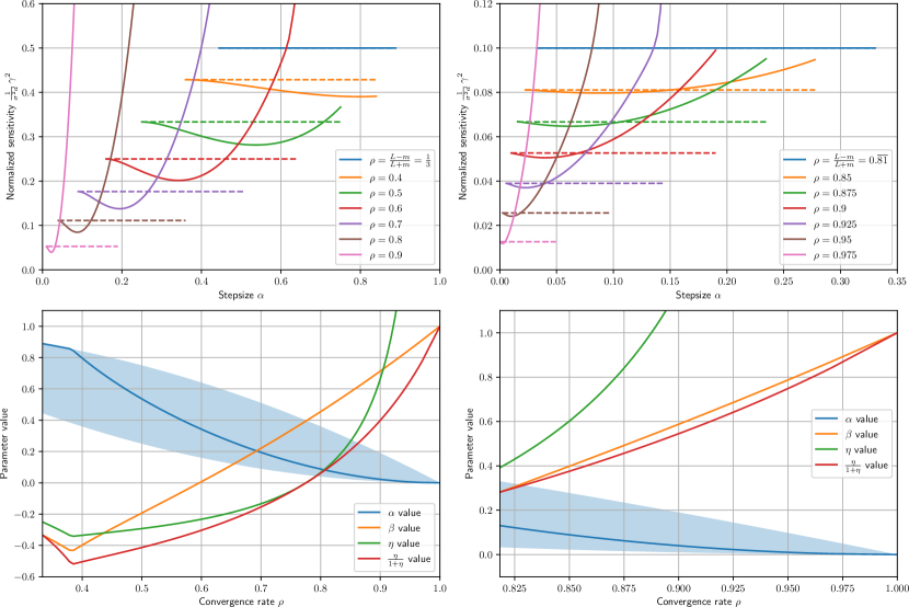
Figure 3: Robust Gradient Descent (RGD) described in 14. The left column is for the function class $S_{1,2}$, and the right column for $S_{1,10}$. The first row shows how choosing $\alpha\in\left[\frac{1}{m}(1-\rho)^{2},\frac{1}{m}(1-\rho^{2})\right]$ for RGD can lead to smaller sensitivity $\gamma$ (solid lines) compared to ordinary GD (dashed lines). The second row shows the range of admissible $\alpha$ values for RGD (shaded region). The solid lines indicate the parameters $(\alpha,\beta,\eta)$ that minimize $\gamma$ in RGD for each value of the convergence rate $\rho$.

A natural question to ask is whether the optimal $\alpha$ and corresponding $\gamma$ bound can be computed analytically for RGD. This is possible in principle, but the solution is too complex to be practical. Starting from the end of the proof of 14 (Section A.6), we can substitute the expressions for $\beta$ and $\eta$ into (19), solve for $P$, and use the stationarity of $\gamma$ to find a first-order optimality condition for $\alpha$. Unfortunately, this condition is a polynomial equation in $(\alpha,\rho)$ with thousands of terms whose leading term in $\alpha$ has degree 224. Thus, it is far more efficient to use a line search to optimize $\alpha$ than to compute it analytically.

5 Smooth strongly convex functions

We now consider the class $F_{m,L}$ of strongly convex functions whose gradient is Lipschitz continuous. A useful characterization of this function class is given by the interpolation conditions, which appeared in [40, Thm. 4]. We state the result here, rephrased to match our notation.

Proposition 16 (Interpolation conditions for $F_{m,L}$).

Let $y_{1},\dots,y_{k}\in\mathbb{R}^{1\times d}$ and $u_{1},\dots,u_{k}\in\mathbb{R}^{1\times d}$ and $f_{1},\dots,f_{k}\in\mathbb{R}$. The following two statements are equivalent.

1. There exists a function $f\in F_{m,L}$ such that $f(y_{i})=f_{i}$ and $\nabla\!f(y_{i})=u_{i}$ for $i=1,\dots,k$.

2. For all $i,j\in\{1,\dots,k\}$,

   $$\operatorname{\mathrm{tr}}\bigl{(}u_{i}^{\mathsf{T}}(y_{i}-y_{j})\bigr{)}+\frac{1}{2\,(L-m)}\operatorname{\mathrm{tr}}\begin{bmatrix}y_{i}-y_{j}\\ u_{i}-u_{j}\end{bmatrix}^{\mathsf{T}}\begin{bmatrix}-mL&m\\ m&-1\end{bmatrix}\begin{bmatrix}y_{i}-y_{j}\\ u_{i}-u_{j}\end{bmatrix}-(f_{i}-f_{j})\geq 0.$$ (20)

If we consider (20) with $(i,j)\mapsto(i,\star)$ and $(i,j)\mapsto(\star,i)$, and sum the resulting two inequalities, then the $f_{i}-f_{\star}$ terms cancel and we recover (17). This verifies the fact that $F_{m,L}\subseteq S_{m,L}$.

5.1 Performance bounds for $F_{m,L}$

Similar to the case $S_{m,L}$, the class of functions $F_{m,L}$ is not readily parameterizable, so we will again adopt a Lyapunov approach to certify performance bounds. Since $F_{m,L}\subseteq S_{m,L}$, we could use 11 to obtain upper bounds on $\rho$ and $\gamma$. However, these bounds would be loose in general because they do not take into account all of the inequalities in (20). To obtain tighter bounds on $\rho$ and $\gamma$ for $F_{m,L}$, we use a lifting approach that allows the Lyapunov function to depend on a finite history of past algorithm iterates and function values.

Lifted dynamics.

The main idea is to lift the state to a higher dimension so that we can use more of the interpolation conditions in searching for a Lyapunov function. We denote the lifting dimension by $\ell\geq 0$, which dictates the dimension of the lifted state, and we use bold to indicate quantities related to the lifted dynamics.

Given a trajectory of the system, we define the following augmented vectors, each consisting of $\ell+1$ consecutive iterates of the system. Recall our convention that algorithm inputs and outputs $u^{t}$, $y^{t}$ are row vectors:

$$\bm{y}^{t} \mathrel{\mathchoice{\vbox{\hbox{$\displaystyle:$}}}{\vbox{\hbox{$\textstyle:$}}}{\vbox{\hbox{$\scriptstyle:$}}}{\vbox{\hbox{$\scriptscriptstyle:$}}}{=}}\begin{bmatrix}y^{t}-y^{\star}\\ \vdots\\ y^{t-\ell}-y^{\star}\end{bmatrix}\in\mathbb{R}^{(\ell+1)\times d}, \bm{u}^{t} \mathrel{\mathchoice{\vbox{\hbox{$\displaystyle:$}}}{\vbox{\hbox{$\textstyle:$}}}{\vbox{\hbox{$\scriptstyle:$}}}{\vbox{\hbox{$\scriptscriptstyle:$}}}{=}}\begin{bmatrix}u^{t}-u^{\star}\\ \vdots\\ u^{t-\ell}-u^{\star}\end{bmatrix}\in\mathbb{R}^{(\ell+1)\times d}, \bm{f}^{t} \mathrel{\mathchoice{\vbox{\hbox{$\displaystyle:$}}}{\vbox{\hbox{$\textstyle:$}}}{\vbox{\hbox{$\scriptstyle:$}}}{\vbox{\hbox{$\scriptscriptstyle:$}}}{=}}\begin{bmatrix}f^{t}-f^{\star}\\ \vdots\\ f^{t-\ell}-f^{\star}\end{bmatrix}\in\mathbb{R}^{\ell+1}.$$ (21)

Also, define the truncation matrices $Z,Z_{+}\in\mathbb{R}^{\ell\times(\ell+1)}$ as

$$Z_{+}\mathrel{\mathchoice{\vbox{\hbox{$\displaystyle:$}}}{\vbox{\hbox{$\textstyle:$}}}{\vbox{\hbox{$\scriptstyle:$}}}{\vbox{\hbox{$\scriptscriptstyle:$}}}{=}}\begin{bmatrix}I_{\ell}&0_{\ell\times 1}\end{bmatrix}\quad\text{and}\quad Z\mathrel{\mathchoice{\vbox{\hbox{$\displaystyle:$}}}{\vbox{\hbox{$\textstyle:$}}}{\vbox{\hbox{$\scriptstyle:$}}}{\vbox{\hbox{$\scriptscriptstyle:$}}}{=}}\begin{bmatrix}0_{\ell\times 1}&I_{\ell}\end{bmatrix}.$$ (22)

Multiplying an augmented vector on the left by $Z$ removes the most recent iterate at time $t$, while multiplication by $Z_{+}$ removes the last iterate at time $t-\ell$. Using these augmented vectors, we then define the augmented state as

$$\bm{x}^{t}\mathrel{\mathchoice{\vbox{\hbox{$\displaystyle:$}}}{\vbox{\hbox{$\textstyle:$}}}{\vbox{\hbox{$\scriptstyle:$}}}{\vbox{\hbox{$\scriptscriptstyle:$}}}{=}}\begin{bmatrix}\xi^{t}-\xi^{\star}\\ Z\bm{y}^{t}\\ Z\bm{u}^{t}\end{bmatrix}\in\mathbb{R}^{(n+2\ell)\times d}$$ (23)

which consists of the current state $\xi^{t}$ as well as the $\ell$ previous inputs $y^{t-1},\ldots,y^{t-\ell}$ and outputs $u^{t-1},\ldots,u^{t-\ell}$ of the original system. Since the dynamics of this augmented state must be consistent with those of the original system, the associated augmented dynamics for the state $\bm{x}^{t}$ with inputs $(\tilde{u}^{t},w^{t})$, which is the same as in (6), and augmented outputs $(\bm{y}^{t},\bm{u}^{t})$ are

$$\bm{x}^{t+1} =\underbrace{\begin{bmatrix}A&0&0\\ Z_{+}\mathsf{e}_{1}C&Z_{+}Z^{\mathsf{T}}&0\\ 0&0&Z_{+}Z^{\mathsf{T}}\end{bmatrix}}_{\bm{A}}\bm{x}^{t}+\underbrace{\begin{bmatrix}B\\ 0\\ Z_{+}\mathsf{e}_{1}\end{bmatrix}}_{\bm{B}}\tilde{u}^{t}+\underbrace{\begin{bmatrix}B\\ 0\\ 0\end{bmatrix}}_{\bm{H}}w^{t},$$ (24a)

$$\begin{bmatrix}\bm{y}^{t}\\ \bm{u}^{t}\end{bmatrix} =\underbrace{\begin{bmatrix}\mathsf{e}_{1}C&Z^{\mathsf{T}}&0\\ 0&0&Z^{\mathsf{T}}\end{bmatrix}}_{\bm{C}}\bm{x}^{t}+\underbrace{\begin{bmatrix}0\\ \mathsf{e}_{1}\end{bmatrix}}_{\bm{D}}\tilde{u}^{t},$$ (24b)

where $\mathsf{e}_{1}=(1,0,\ldots,0)\in\mathbb{R}^{\ell+1}$. We can recover the iterates of the original system by projecting the augmented state and the input as

$$\tilde{\xi}^{t} =\underbrace{\begin{bmatrix}I_{n}&0_{n\times(2\ell+1)}\end{bmatrix}}_{\bm{X}}\begin{bmatrix}\bm{x}^{t}\\ \tilde{u}^{t}\end{bmatrix}, \tilde{y}^{t} =\underbrace{\begin{bmatrix}C&0_{1\times(2\ell+1)}\end{bmatrix}}_{\bm{Y}}\begin{bmatrix}\bm{x}^{t}\\ \tilde{u}^{t}\end{bmatrix}, \tilde{u}^{t} =\underbrace{\begin{bmatrix}0_{1\times(n+2\ell)}&1\end{bmatrix}}_{\bm{U}}\begin{bmatrix}\bm{x}^{t}\\ \tilde{u}^{t}\end{bmatrix}.$$ (25)

State reduction for the noise-free case.

When there is no noise ($w^{t}=0$), the augmented state (23) has linearly dependent rows. This leads to the definition of a reduced state $\bm{x}_{r}^{t}\in\mathbb{R}^{(n+\ell)\times d}$

$$\bm{x}^{t}=\begin{bmatrix}\tilde{\xi}^{t}\\ Z\bm{y}^{t}\\ Z\bm{u}^{t}\end{bmatrix}=\left[\begin{array}[]{c:cccc}A^{\ell}&B&AB&\cdots&A^{\ell-1}B\rule{0.0pt}{11.19443pt}\rule[-3.87495pt]{0.0pt}{0.0pt}\\ \hdashline CA^{\ell-1}&0&CB&\cdots&CA^{\ell-2}B\rule{0.0pt}{11.19443pt}\\ \vdots&&0&\ddots&\vdots\\ CA&&&\ddots&CB\\ C&&&&0\\ \hdashline 0_{\ell\times 1}&\lx@intercol\hfil I_{\ell}\hfil\lx@intercol\rule{0.0pt}{11.19443pt}\rule[-3.87495pt]{0.0pt}{0.0pt}\end{array}\right]\!\begin{bmatrix}\tilde{\xi}^{t-\ell}\\ Z\bm{u}^{t}\end{bmatrix}\,\mathrel{{=}\mathchoice{\vbox{\hbox{$\displaystyle:$}}}{\vbox{\hbox{$\textstyle:$}}}{\vbox{\hbox{$\scriptstyle:$}}}{\vbox{\hbox{$\scriptscriptstyle:$}}}}\Psi\,\bm{x}_{r}^{t}.$$ (26)

The associated augmented (noise-free) dynamics for this reduced state are

$$\bm{x}_{r}^{t+1} =\underbrace{\begin{bmatrix}A&B\mathsf{e}_{\ell+1}^{\mathsf{T}}Z^{\mathsf{T}}\\ 0&Z_{+}Z^{\mathsf{T}}\end{bmatrix}}_{\bm{A}_{r}}\bm{x}_{r}^{t}+\underbrace{\begin{bmatrix}0\\ Z_{+}\mathsf{e}_{1}\end{bmatrix}}_{\bm{B}_{r}}\tilde{u}^{t},$$ (27a)

$$\begin{bmatrix}\bm{y}^{t}\\ \bm{u}^{t}\end{bmatrix} =\underbrace{\begin{bmatrix}\mathsf{e}_{1}C\Psi_{11}+Z^{\mathsf{T}}\Psi_{21}&\mathsf{e}_{1}C\Psi_{12}+Z^{\mathsf{T}}\Psi_{22}\\ 0&Z^{\mathsf{T}}\end{bmatrix}}_{\bm{C}_{r}}\bm{x}_{r}^{t}+\underbrace{\begin{bmatrix}0\\ \mathsf{e}_{1}\end{bmatrix}}_{\bm{D}_{r}}\tilde{u}^{t},$$ (27b)

where $\mathsf{e}_{\ell+1}=(0,0,\ldots,1)\in\mathbb{R}^{\ell+1}$ and $\Psi_{ij}$ denotes the $(i,j)$ block of the $3\times 2$ block-matrix $\Psi$ defined in (26). We can recover the iterates of the original system as before, using

$$\tilde{\xi}^{t} =\underbrace{\begin{bmatrix}\Psi_{11}&\Psi_{12}&0_{n\times 1}\end{bmatrix}}_{\bm{X}_{r}}\begin{bmatrix}\bm{x}_{r}^{t}\\ \tilde{u}^{t}\end{bmatrix}, \tilde{y}^{t} =\underbrace{\begin{bmatrix}C\Psi_{11}&C\Psi_{12}&0\end{bmatrix}}_{\bm{Y}_{r}}\begin{bmatrix}\bm{x}_{r}^{t}\\ \tilde{u}^{t}\end{bmatrix}, \tilde{u}^{t} =\underbrace{\begin{bmatrix}0_{1\times(n+\ell)}&1\end{bmatrix}}_{\bm{U}_{r}}\begin{bmatrix}\bm{x}_{r}^{t}\\ \tilde{u}^{t}\end{bmatrix}.$$ (28)

We now develop a version of 16 that holds for the augmented vectors defined above. The proof is provided in Section A.7.

Lemma 17.

Consider a function $f\in F_{m,L}$, and let $y^{\star}\in\mathbb{R}^{1\times d}$ denote the optimizer, $u^{\star}=0\in\mathbb{R}^{1\times d}$ the optimal gradient, and $f^{\star}\in\mathbb{R}$ the optimal value. Let $y^{t},\dots,y^{t-\ell}\in\mathbb{R}^{1\times d}$ be a sequence of iterates, and define $u^{t-i}\mathrel{\mathchoice{\vbox{\hbox{$\displaystyle:$}}}{\vbox{\hbox{$\textstyle:$}}}{\vbox{\hbox{$\scriptstyle:$}}}{\vbox{\hbox{$\scriptscriptstyle:$}}}{=}}\nabla\!f(y^{t-i})$ and $f^{t-i}\mathrel{\mathchoice{\vbox{\hbox{$\displaystyle:$}}}{\vbox{\hbox{$\textstyle:$}}}{\vbox{\hbox{$\scriptstyle:$}}}{\vbox{\hbox{$\scriptscriptstyle:$}}}{=}}f(y^{t-i})$ for $i=0,\dots,\ell$. Using these values, define the augmented vectors $\bm{y}^{t}$, $\bm{u}^{t}$, $\bm{f}^{t}$ as in (21). Finally, define the index set $I\mathrel{\mathchoice{\vbox{\hbox{$\displaystyle:$}}}{\vbox{\hbox{$\textstyle:$}}}{\vbox{\hbox{$\scriptstyle:$}}}{\vbox{\hbox{$\scriptscriptstyle:$}}}{=}}\{1,\ldots,\ell+1,\star\}$ and let $\mathsf{e}_{i}$ denote the $i\textsuperscript{th}$ unit vector in $\mathbb{R}^{\ell+1}$ with $\mathsf{e}_{\star}\mathrel{\mathchoice{\vbox{\hbox{$\displaystyle:$}}}{\vbox{\hbox{$\textstyle:$}}}{\vbox{\hbox{$\scriptstyle:$}}}{\vbox{\hbox{$\scriptscriptstyle:$}}}{=}}0\in\mathbb{R}^{\ell+1}$. Then the inequality

$$\operatorname{\mathrm{tr}}\begin{bmatrix}\bm{y}^{t}\\ \bm{u}^{t}\end{bmatrix}^{\mathsf{T}}\Pi(\Lambda)\begin{bmatrix}\bm{y}^{t}\\ \bm{u}^{t}\end{bmatrix}+\pi(\Lambda)^{\mathsf{T}}\bm{f}^{t}\geq 0$$ (29)

holds for all $\Lambda\in\mathbb{R}^{(\ell+2)\times(\ell+2)}$ such that $\Lambda\geq 0$ (pointwise), where

$$\Pi(\Lambda) =\sum_{i,j\in I}\Lambda_{ij}\begin{bmatrix}-mL\,(\mathsf{e}_{i}-\mathsf{e}_{j})(\mathsf{e}_{i}-\mathsf{e}_{j})^{\mathsf{T}}&(\mathsf{e}_{i}-\mathsf{e}_{j})(m\mathsf{e}_{i}-L\mathsf{e}_{j})^{\mathsf{T}}\\[2.0pt] (m\mathsf{e}_{i}-L\mathsf{e}_{j})(\mathsf{e}_{i}-\mathsf{e}_{j})^{\mathsf{T}}&-(\mathsf{e}_{i}-\mathsf{e}_{j})(\mathsf{e}_{i}-\mathsf{e}_{j})^{\mathsf{T}}\end{bmatrix},$$ (30a)

$$\pi(\Lambda) =2\,(L-m)\sum_{i,j\in I}\Lambda_{ij}\,(\mathsf{e}_{i}-\mathsf{e}_{j}).$$ (30b)

Just as in the sector-bounded case, our analysis is based on searching for a function that certifies either a particular worst-case rate $\rho$ (assuming no noise) or a level of sensitivity $\gamma$ (assuming noise). The difference is that the function now depends on the lifted state as well as the augmented vector of function values, that is, we search for certificates of the form

$$V(\bm{x},\bm{f})\mathrel{\mathchoice{\vbox{\hbox{$\displaystyle:$}}}{\vbox{\hbox{$\textstyle:$}}}{\vbox{\hbox{$\scriptstyle:$}}}{\vbox{\hbox{$\scriptscriptstyle:$}}}{=}}\operatorname{\mathrm{tr}}\bigl{(}\bm{x}^{\mathsf{T}}P\bm{x}\bigr{)}+p^{\mathsf{T}}Z\bm{f}.$$ (31)

This is quadratic in the lifted state and linear in the $\ell$ previous function values. Here, the lifted state is either $\bm{x}^{t}$ defined in (23) or the reduced state $\bm{x}_{r}^{t}$ defined in (26), depending on whether there is noise or not, respectively.

The conditions that this certificate must satisfy are then similar to the sector-bounded case. To certify convergence, we search for a function that satisfies the following conditions for all trajectories of the noise-free dynamics.

• Lower bound condition: $V(\bm{x}_{r}^{t},\bm{f}^{t})\geq\lVert{\xi^{t}-\xi^{\star}}\rVert^{2}$

• Decrease condition: $V(\bm{x}_{r}^{t+1},\bm{f}^{t+1})\leq\rho^{2}\,V(\bm{x}_{r}^{t},\bm{f}^{t})$ for some fixed $\rho>0$

These conditions imply that $\lVert{\xi^{t}-\xi^{\star}}\rVert^{2}\leq\rho^{2t}\,V(\bm{x}_{r}^{0},\bm{f}^{0})$, and therefore provide a way to certify convergence with a given rate $\rho$. To bound the sensitivity of an algorithm to noise, we search for a certificate that satisfies the following.

• Lower bound condition: $\operatorname{\mathbb{E}}V(\bm{x}^{t},\bm{f}^{t})\geq 0$

• Increment condition: $\operatorname{\mathbb{E}}V(\bm{x}^{t+1},\bm{f}^{t+1})-\operatorname{\mathbb{E}}V(\bm{x}^{t},\bm{f}^{t})+\operatorname{\mathbb{E}}\,\lVert{y^{t}-y^{\star}}\rVert^{2}\leq\gamma^{2}$ for some fixed $\gamma>0$

These conditions imply that $0\leq\frac{1}{T}\operatorname{\mathbb{E}}V(\bm{x}^{T},\bm{f}^{T})\leq\frac{1}{T}\operatorname{\mathbb{E}}V(\bm{x}^{0},\bm{f}^{0})+\operatorname{\mathbb{E}}\sum_{t=0}^{T-1}\lVert{y^{t}-y^{\star}}\rVert^{2}\leq\gamma^{2}$ and therefore if we let $T\to\infty$ we have that $\gamma$ is an upper bound on the senstivity to gradient noise.

Since $V$ is quadratic in the augmented state and linear in the augmented function values, we can efficiently search for such Lyapunov functions using the following linear matrix inequalities that make use of the characterization of smooth strongly convex functions in 17. The proof is provided in Section A.8

Theorem 18 ($F_{m,L}$ analysis).

Consider an algorithm $\mathcal{A}=(A,B,C)$ defined in (6) satisfying 2 applied to a function $f\in F_{m,L}$ defined in Section 1 with additive gradient noise with covariance bound $\sigma^{2}I_{d}$. Define the truncation matrices in (22), the augmented state space and projection matrices in (24)–(28), and the multiplier functions in (30). Then the algorithm satisfies the following convergence rate and robustness bounds.

1. If there exist $P=P^{\mathsf{T}}\in\mathbb{R}^{(n+\ell)\times(n+\ell)}$ and $p\in\mathbb{R}^{\ell}$ and $\Lambda_{1},\Lambda_{2}\geq 0$ and $\rho>0$ such that

   $$\begin{bmatrix}\bm{A}_{r}&\bm{B}_{r}\\ I&0\end{bmatrix}^{\mathsf{T}}\begin{bmatrix}P&0\\ 0&-\rho^{2}P\end{bmatrix}\begin{bmatrix}\bm{A}_{r}&\bm{B}_{r}\\ I&0\end{bmatrix}+\begin{bmatrix}\bm{C}_{r}&\bm{D}_{r}\end{bmatrix}^{\mathsf{T}}\Pi(\Lambda_{1})\begin{bmatrix}\bm{C}_{r}&\bm{D}_{r}\end{bmatrix} \preceq 0$$ (32a)

   $$(Z_{+}-\rho^{2}Z)^{\mathsf{T}}p+\pi(\Lambda_{1}) \leq 0$$ (32b)

   $$\bm{X}_{r}^{\mathsf{T}}\bm{X}_{r}-\begin{bmatrix}I&0\end{bmatrix}^{\mathsf{T}}P\begin{bmatrix}I&0\end{bmatrix}+\begin{bmatrix}\bm{C}_{r}&\bm{D}_{r}\end{bmatrix}^{\mathsf{T}}\Pi(\Lambda_{2})\begin{bmatrix}\bm{C}_{r}&\bm{D}_{r}\end{bmatrix} \preceq 0$$ (32c)

   $$-Z^{\mathsf{T}}p+\pi(\Lambda_{2}) \leq 0$$ (32d)

   then $\rho(\mathcal{A},F_{m,L})\leq\rho$.

2. If there exist $P=P^{\mathsf{T}}\in\mathbb{R}^{(n+2\ell)\times(n+2\ell)}$ and $p\in\mathbb{R}^{\ell}$ and $\Lambda_{1},\Lambda_{2}\geq 0$ such that

   $$\begin{bmatrix}\bm{A}&\bm{B}\\ I&0\end{bmatrix}^{\mathsf{T}}\begin{bmatrix}P&0\\ 0&-P\end{bmatrix}\begin{bmatrix}\bm{A}&\bm{B}\\ I&0\end{bmatrix}+\begin{bmatrix}\bm{C}&\bm{D}\end{bmatrix}^{\mathsf{T}}\Pi(\Lambda_{1})\begin{bmatrix}\bm{C}&\bm{D}\end{bmatrix}+\bm{Y}^{\mathsf{T}}\bm{Y} \preceq 0$$ (33a)

   $$(Z_{+}-Z)^{\mathsf{T}}p+\pi(\Lambda_{1}) \leq 0$$ (33b)

   $$-\begin{bmatrix}I&0\end{bmatrix}^{\mathsf{T}}P\begin{bmatrix}I&0\end{bmatrix}+\begin{bmatrix}\bm{C}&\bm{D}\end{bmatrix}^{\mathsf{T}}\Pi(\Lambda_{2})\begin{bmatrix}\bm{C}&\bm{D}\end{bmatrix} \preceq 0$$ (33c)

   $$-Z^{\mathsf{T}}p+\pi(\Lambda_{2}) \leq 0$$ (33d)

   then $\gamma(\mathcal{A},F_{m,L},\sigma^{2})\leq\sqrt{\sigma^{2}d\cdot(\bm{H}^{\mathsf{T}}P\bm{H})}$.

Remark 19.

When the lifting dimension $\ell$ is zero, the lifted system is identical to the original system. In other words, $\tilde{\xi}^{t}=\bm{x}^{t}=\bm{x}_{r}^{t}$. The system matrices also satisfy $A=\bm{A}=\bm{A}_{r}$, and similarly for $B$. In this case, the Lyapunov function in (31) is the same as that used for the $S_{m,L}$ case, and the analysis reduces to that of 11. As $\ell$ is increased, the LMIs (32) and (33) have the potential to yield less conservative bounds on $\rho$ and $\gamma$, respectively.

Remark 20.

In 18, the LMI (32) has fewer inequalities and variables than the LMI (33) because it makes use of the reduced state $\bm{x}_{r}^{t}$ instead of the full state $\bm{x}^{t}$. The reduced state can only be used when computing $\rho$ because this case has no noise.

As with the $S_{m,L}$ LMIs of 11, both bounds for the class $F_{m,L}$ in 18 can be evaluated and optimized efficiently. Again, the sizes of the LMIs depend only on $n$ and $\ell$, which are typically small. The choice of $\ell$ is addressed in Section 5.2 when we present our algorithm design.

5.2 Algorithm design for $F_{m,L}$

For the case with no noise, the Triple Momentum (TM) method [42] attains the fastest-known worst-case rate of $\rho_{\text{TM}}=1-\sqrt{\frac{m}{L}}$ over the function class $F_{m,L}$. It has recently been shown that this rate cannot be improved using Zames–Falb multipliers from robust control [38].

There are few examples in the literature of accelerated algorithms that trade off convergence rate and sensitivity to noise via explicit parameter tuning. One example is the Robust Momentum (RM) method, proposed in [10], which uses the parameter $\rho\in\bigl{[}1-\sqrt{\frac{m}{L}},1-\frac{m}{L}\bigr{]}$. When $\rho=1-\sqrt{\frac{m}{L}}$, RM recovers TM (fast but sensitive to noise). When $\rho=1-\frac{m}{L}$, RM recovers GD with stepsize $\alpha=\frac{1}{L}$ (slow, but robust to noise). The RM algorithm was designed for use with multiplicative noise and does not perform as well with additive noise.

We adopted the three-parameter class $(\alpha,\beta,\eta)$ described in Section 2.2 as our search space for optimized algorithms, because it includes TM and RM as special cases, as well Nesterov’s Fast Gradient (FG) method, which is a popular choice for this function class. Our proposed algorithm, which we call the Robust Accelerated Method (RAM), uses a parameter $\rho$ similar to RM to trade off convergence rate and sensitivity to noise, but achieves better performance than RM in the sense that it is closer to being Pareto-optimal.

To design RAM, we followed the procedure outlined in Section 1.3. Using the weighted off-by-one IQC formulation (34) (in the following subsection) parameterized by the matrix $Q$, the matrix in the LMI (32a) has rank one, so all of its $2\times 2$ minors are zero. Furthermore, the vector in the inequality (32b) is zero. We then solved this set of polynomial equations for the algorithm stepsizes and the solution to the LMI, using the values of a numerically-optimized algorithm to guide the solution process. Our main result concerning RAM is 21, whose proof is in Section A.9.

Theorem 21 (Robust Accelerated Method, RAM).

Consider the function class $F_{m,L}$, and let $\rho$ be a parameter chosen with $1-\sqrt{\frac{m}{L}}\leq\rho<1$. Then, the algorithm $\mathcal{A}$ of the form (5) with tuning

$$\alpha=\frac{(1+\rho)(1-\rho)^{2}}{m}, \beta=\rho\,\frac{L\,(1-\rho+2\rho^{2})-m\,(1+\rho)}{(L-m)(3-\rho)}, \eta=\rho\,\frac{L\,(1-\rho^{2})-m\,(1+2\rho-\rho^{2})}{(L-m)(3-\rho)(1-\rho^{2})}$$

achieves the performance metric $\rho(\mathcal{A},F_{m,L})=\rho$.

Remark 22.

When the convergence factor $\rho$ is set to its minimum value of $1-\sqrt{\frac{m}{L}}$, the Robust Accelerated Method in 21 reduces to the Triple Momentum Method (see Table 1).

5.3 Comparison with other approaches

We now compare our analysis in 18 with several other approaches in the literature for computing the convergence rate and sensitivity for the function class $F_{m,L}$.

One alternative approach is to use integral quadratic constraints [28] from robust control. Consider the LMI in [26, Eq. 3.8] with the weighted off-by-one IQC in [26, Lemma 10], which is parameterized by $\rho$. Feasibility of this LMI certifies that $\rho$ is an upper bound on the convergence rate. Suppose that the LMI is feasible for some positive definite $Q\succ 0$ (assuming $\lambda=1$ without loss of generality). Then our analysis LMI (32) has the feasible solution

$$p=2\,(L-m),\quad\Lambda_{1}=\begin{bmatrix}0&0&0\\ \rho^{2}&0&0\\ 1-\rho^{2}&0&0\end{bmatrix},\quad\Lambda_{2}=\begin{bmatrix}0&0&0\\ 0&0&1\\ 0&0&0\end{bmatrix},\quad\text{and}$$ (34a)

$$P=\begin{bmatrix}A&B\\ -LC&1\end{bmatrix}^{\mathsf{T}}Q\begin{bmatrix}A&B\\ -LC&1\end{bmatrix}-(L-m)\,m\begin{bmatrix}C^{\mathsf{T}}C&0\\ 0&0\end{bmatrix}-\begin{bmatrix}-mC&1\end{bmatrix}^{\mathsf{T}}\begin{bmatrix}-mC&1\end{bmatrix}.$$ (34b)

In this case, a Lyapunov function for the system is

$$V^{t}=\begin{bmatrix}\tilde{x}^{t}\\ \tilde{\zeta}^{t}\end{bmatrix}^{\mathsf{T}}\!Q\begin{bmatrix}\tilde{x}^{t}\\ \tilde{\zeta}^{t}\end{bmatrix}+2\,(L-m)\left(\tilde{f}^{t-1}-\frac{m}{2}\bigl{\lVert}{\tilde{y}^{t-1}}\bigr{\rVert}^{2}\right)-\bigl{\lVert}{\tilde{u}^{t-1}-m\tilde{y}^{t-1}}\bigr{\rVert}^{2}$$ (35)

where $\tilde{\zeta}^{t}\mathrel{\mathchoice{\vbox{\hbox{$\displaystyle:$}}}{\vbox{\hbox{$\textstyle:$}}}{\vbox{\hbox{$\scriptstyle:$}}}{\vbox{\hbox{$\scriptscriptstyle:$}}}{=}}\tilde{u}^{t-1}-L\tilde{y}^{t-1}$. Therefore, using the weighted off-by-one IQC can be interpreted as searching over this restricted class of Lyapunov functions. Even though our analysis for computing the convergence rate in 18 is more general, the weighted off-by-one IQC formulation appears to be general enough to prove tight results. For example, while RAM was designed using the more general analysis, its Lyapunov function has the special form (35); see Section A.9.

In the recent work [29], Zames–Falb multipliers [44] are used to formulate LMIs for computing both the convergence rate and the sensitivity (the weighted off-by-one IQC is a special case of the more general Zames–Falb multipliers). Just as with the weighted off-by-one IQC, using general Zames–Falb multipliers can also be interpreted as searching over a restricted class of Lyapunov functions, although a detailed comparison is beyond the scope of this work.

While the weighted off-by-one IQC formulation appears to achieve tight bounds on the convergence rate, computing tight bounds on the sensitivity requires the more general LMI (33); see Table 3.

6 Numerical validation

In this section, we use numerical experiments to verify that our algorithm designs: achieve a near-optimal trade-off between convergence rate and noise robustness, have optimal asymptotic convergence, use an adequate number of parameters (they are neither under- nor over-parameterized), and outperform popular iterative schemes when applied to a worst-case test function.

6.1 Empirical verification of near-optimality

The main results of the previous sections provided means to efficiently compute upper bounds on the worst-case convergence rate $\rho$ and sensitivity $\gamma$ for any algorithm in our three-parameter family $\mathcal{A}=(\alpha,\beta,\eta)$. We also provided near-optimal designs for the function classes $Q_{m,L}$, $S_{m,L}$, and $F_{m,L}$. Table 2 summarizes these results.

Table 2: Summary of analysis and design results from Sections 3 to 5.

Function class	Analysis result ($\rho$ and $\gamma$)	Algorithm design
$Q_{m,L}$ (strongly convex quadratics),	Section 3, 8	RHB, 9
$S_{m,L}$ (one-point strong convexity),	Section 4, 11	RGD, 14
$F_{m,L}$ (strong convexity)	Section 5, 18	RAM, 21

To empirically validate the near-optimality of our designs, we can perform a brute-force search over algorithms $(\alpha,\beta,\eta)$ and make a scatter plot of the performance $(\rho,\gamma)$ to see where our designs lie compared to the Pareto-optimal front. To facilitate sampling, the following result provides bounds on admissible tuples $(\alpha,\beta,\eta)$.

Lemma 23 (algorithm parameter restriction).

Consider the three-parameter algorithm $\mathcal{A}=(\alpha,\beta,\eta)$ defined in Section 2.2. Let $\mathcal{F}\in\{Q_{m,L},F_{m,L},S_{m,L}\}$. If $\rho(\mathcal{A},\mathcal{F})<1$, then:

$$0<\alpha<\frac{4}{L},\qquad\frac{-2}{L-m}<\alpha\eta<\frac{2}{L-m},\quad\text{and}\quad\begin{cases}-1+L(\alpha\eta)<\beta<1+m(\alpha\eta)&\text{if }\alpha\eta\geq 0\\ -1+m(\alpha\eta)<\beta<1+L(\alpha\eta)&\text{if }\alpha\eta<0.\end{cases}$$

From 23, we see that $(\alpha,\alpha\eta,\beta)$ each have finite ranges. So a convenient way to grid the space of possible $(\alpha,\beta,\eta)$ values is to first grid over $\alpha$, then $\alpha\eta$, then $\beta$, in a nested fashion, extracting the associated $(\alpha,\beta,\eta)$ values at each step. Due to the multiplicative nature of the parameter $\alpha$, we opted to sample $\alpha$ logarithmically in the range $\bigl{[}10^{-5},\tfrac{4}{L}\bigr{]}$, but to sample $\alpha\eta$ and $\beta$ linearly in their associated intervals.

Strongly convex quadratics ($Q_{m,L}$).

We show our brute-force search for the class $Q_{m,L}$ in Fig. 4 for $Q_{1,10}$ and $Q_{1,100}$. For this figure, we used the sampling approach described in 23 with $500\times 201\times 200$ samples for $(\alpha,\alpha\eta,\eta)$.

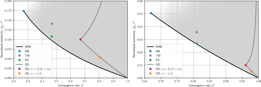
Figure 4: Plot of $\gamma^{2}$ vs. $\rho^{2}$ for algorithms applied to the function class $Q_{1,10}$ (left panel) and $Q_{1,100}$ (right panel), found using 8. Each point in the point cloud corresponds to an algorithm $(\alpha,\beta,\eta)$. The Pareto-optimal front coincides with the Robust Heavy Ball method (9), tuned using $\rho\in\left[\frac{\sqrt{L}-\sqrt{m}}{\sqrt{L}+\sqrt{m}},1\right]$ to mediate the trade-off.

In Fig. 4, each algorithm $(\alpha,\beta,\eta)$ corresponds to a single gray dot. The curve labeled RHB shows each possible tuning as we vary the parameter $\rho$. We observe that RHB perfectly traces out the boundary of the point cloud, which represents the Pareto-optimal algorithms. In other words, for a fixed convergence rate $\rho$, RHB with parameter $\rho$ achieves this rate and is also as robust as possible to additive gradient noise (smallest $\gamma$).

Fig. 4 reveals that Gradient Descent (GD) with $0<\alpha<\tfrac{2}{L+m}$ is outperformed by by RHB on the function class $Q_{m,L}$. We also plot the performance of GD for $\alpha>\tfrac{2}{L+m}$, which is even worse as this leads to slower convergence and increased sensitivity. Fig. 4 also reveals that the Fast Gradient (FG) method is strictly suboptimal compared to RHB, although the optimality gap appears to shrink as $L/m$ gets larger.

One-point strong convexity ($S_{m,L}$).

We show our brute-force search for the class $S_{m,L}$ in Fig. 5 for $Q_{1,2}$ and $Q_{1,10}$. For this figure, we used the same sampling approach as in Fig. 4, but with $200\times 51\times 50$ samples this time.

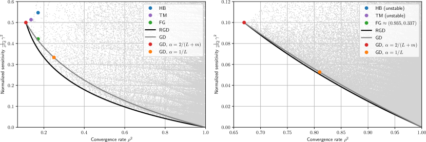
Figure 5: Plot of $\gamma^{2}$ vs. $\rho^{2}$ for algorithms applied to the function class $S_{1,2}$ (left panel) and $S_{1,10}$ (right panel), found using 11. Each point in the point cloud corresponds to an algorithm $(\alpha,\beta,\eta)$. GD is strictly suboptimal, and the Pareto-optimal front closely matches RGD (14), tuned using $\rho\in\bigl{[}\frac{L-m}{L+m},1\bigr{]}$ to mediate the trade-off and with $\alpha$ optimized via line search for each $\rho$.

We used smaller $L$ values for this function class in order to highlight the performance gap between our proposed Robust Gradient Descent (RGD) and ordinary Gradient Descent (GD). As $L/m$ gets larger, this gap shrinks and the performance of RGD becomes indistinguishable from that of GD. For clarity, we also omitted the plots for GD with $\alpha>\frac{2}{L+m}$.

Although the numerical evidence in Fig. 5 suggests that RGD is Pareto-optimal, it is not. RGD is strictly suboptimal, but the optimality gap is so small that it is not visible on the plot. As an example, consider RGD with the parameter choice $\rho=0.9$, $m=1$, $L=2$, $d=1$, $\sigma=1$. Using a line search to optimize the RGD method from 14 (finding the $\alpha$ that yields the smallest $\gamma$), we obtain: $(\alpha,\beta,\eta)=(0.022382,0.713410,0.663514)$. The associated performance found via 11 with a bisection search to optimize $\rho$ yields: $\rho=0.9000$ and $\gamma=0.1981$ (all digits significant). We applied the Nelder–Mead algorithm directly on the parameters $(\alpha,\beta,\eta)$ to see if RGD was locally optimal. We found that using $(\alpha,\beta,\eta)=(0.022264,0.705943,0.209322)$ yielded the performance $\rho=0.9000$ and $\gamma=0.1974$ (all digits significant). This numerically obtained algorithm is strictly superior (same $\rho$ but smaller $\gamma$) to RGD.

Smooth strongly convex functions ($F_{m,L}$).

We show our brute-force search for the class $F_{m,L}$ in Fig. 6 for $F_{1,10}$ and $F_{1,100}$. For this figure, we used the same sampling approach as in Figs. 4 and 5, with $200\times 51\times 50$ samples. When applying 18, we used a lifting dimension $\ell=1$ to compute $\rho$ and $\ell=6$ to compute $\gamma$. For more details on these choices, see Appendix B.

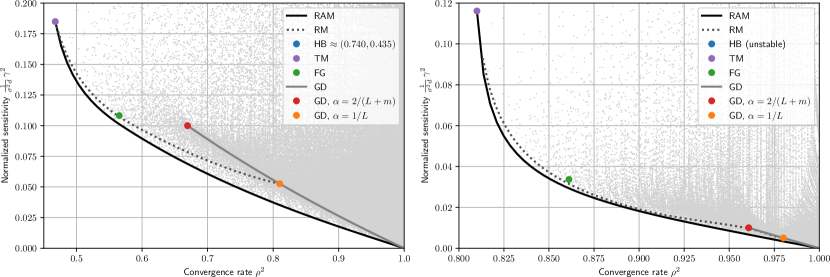
Figure 6: Plot of $\gamma^{2}$ vs. $\rho^{2}$ for algorithms applied to the function class $F_{1,10}$ (left panel) and $F_{1,100}$ (right panel), found using 18. Each point in the point cloud corresponds to an algorithm $(\alpha,\beta,\eta)$. We used a lifting dimension $\ell=1$ for computing $\rho$ and $\ell=6$ for computing $\gamma$. RM and GD are strictly suboptimal, and the Pareto-optimal front closely matches RAM (21), tuned using $\rho\in\left[1-\sqrt{\frac{m}{L}},1\right]$ to mediate the trade-off.

The Robust Momentum (RM) method from [10] interpolates between TM and GD with $\alpha=\frac{1}{L}$ and does trade off convergence rate for sensitivity, but it is strictly outperformed by our proposed Robust Accelerated Method (RAM). The gap in performance between RM and RAM appears to shrink as $L/m$ gets larger.

As with RGD, Fig. 6 suggests that RAM is Pareto-optimal. However, RAM is strictly suboptimal. Suboptimality becomes most apparent when $L/m$ is small and $\rho$ is close to $1$. For example, consider RAM with the parameter choice $\rho=0.9$, $m=1$, $L=2$, $d=1$, $\sigma=1$, which corresponds to $(\alpha,\beta,\eta)=(0.019,0.66,-3.631579)$. Solving the LMIs in 18 yields the bounds $(\rho,\gamma)=(0.9000,0.22057)$. However, if we change $\eta$ and use the tuning $(\alpha,\beta,\eta)=(0.019,0.66,0.00)$ instead, we obtain $(\rho,\gamma)=(0.9000,0.1676)$, so $\rho$ is the same but $\gamma$ is strictly better. Larger optimality gaps can be found by making $L/m$ even closer to $1$, however such cases are not practical.

Remark 24.

The point cloud in the left panel of Fig. 6 ($L/m=10$) is denser than that of the right panel ($L/m=100$), even though the same number of sample points is used in both experiments. The reason for this difference is that the point cloud on the right is spread over a relatively larger range of $\gamma$ values (we truncated the vertical axis). In other words, desirable algorithm tunings are harder to find by random sampling when $L/m$ is larger.

6.2 Verification of optimal asymptotic convergence rate

Figs. 4 to 6 show that as $\rho\to 1$, we have $\gamma\to 0$. So in the limit of slow convergence, we obtain the desirable behavior of complete noise attenuation. However, these trade-off plots give limited insight on the asymptotic convergence rate as $\rho\to 1$. As mentioned in Section 1.2, the fastest possible convergence rate for the mean squared error of any algorithm is $1/t$. Therefore, for any fixed initial condition and objective function, there must exist some constant $c_{0}>0$ such that

$$\mathbb{E}\,\lVert{y^{t}-y^{\star}}\rVert^{2}>\frac{c_{0}}{t+1}\quad\text{for all $t\geq 0$.}$$ (36)

We are interested in the asymptotic behavior $(\rho,\gamma)\to(1,0)$. The convergence behavior of any fixed tuning will look like $\mathbb{E}\,\lVert{y^{t}-y^{\star}}\rVert^{2}=\max\{c_{1}^{2}\gamma^{2}\rho^{2t},\gamma^{2}\}$ (as in Fig. 1), where $c_{1}>1$ is determined by the initial condition. The phase transition occurs when $c_{1}\rho^{t}=1$. In other words, $t=\frac{\log c_{1}}{-\log\rho}$. Substituting $t$ into (36) and rearranging the inequality assuming $0<\rho<1$, we obtain

$$\gamma^{2}\left(\frac{-1}{\log\rho}\right)>\frac{c_{0}}{\log c_{1}-\log\rho}\,\xrightarrow{\rho\to 1}\,\frac{c_{0}}{\log c_{1}}>0.$$

The quantity $-1/\log\rho$ may be interpreted as the iteration complexity; it is proportional to the number of iterations required to guarantee that the error is less than some prescribed amount. For an algorithm with optimal scaling as $\rho\to 1$, a log-log plot of $\gamma^{2}$ vs. $-1/\log\rho$ is therefore a line of slope $-1$ as $\rho\to 1$. As shown in Fig. 7, our algorithm designs appear to have optimal or near-optimal scaling as $\rho\to 1$. An asymptotic slope steeper than $-1$ is not possible, for then a rate faster than $1/t$ could be achieved with a suitably chosen piecewise constant $\rho$ schedule.

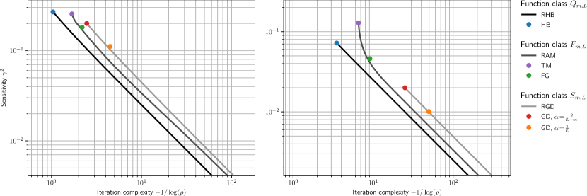
Figure 7: The same data as Fig. 2, except we plot iteration complexity $-1/\log(\rho)$ on the $x$-axis and the plot is on a log-log scale. All proposed algorithms have a slope of $-1$, which matches the optimal rate of $1/t$ achievable by gradient descent with decaying stepsize.

For cases where we have an explicit formula for $\gamma$ in terms of $\rho$ such as for GD (13) and RHB (9), we can evaluate $\lim_{\rho\to 1^{-}}\gamma^{2}(-1/\log\rho)$ and as expected, it is finite in both cases, equal to $\frac{1}{2}$ and $\frac{1}{4}$, respectively.

6.3 Justification for the three-parameter algorithm family

A natural question to ask is whether something as general as our three-parameter family (5) is needed to achieve optimal Pareto-optimal designs. Several recent works have restricted their attention to optimizing algorithms with two parameters $(\alpha,\beta)$ in either Nesterov’s FG or Polyak’s HB form [5, 31, 20]. From our results in Sections 3.2 and 6.1, the HB form is sufficient for the class $Q_{m,L}$. However, neither the HB or the FG forms are sufficient for $F_{m,L}$. While some algorithms in these restricted classes achieve acceleration, they are incapable of obtaining the Pareto-optimal trade-off between convergence rate and sensitivity, as illustrated in Fig. 8 (left panel). Indeed, even when there is no noise, no algorithm in the FG or HB families achieves the optimal convergence rate for the function class $F_{m,L}$, which is attained by Van Scoy et al.’s Triple Momentum (TM) method [42].

Alternatively, we could ask whether three parameters are enough, and whether adding more could lead to further improvements. As explained in Section 2.2, any algorithm with $n=2$ states can be represented by three parameters. In general, we would need $2n-1$ parameters to represent an algorithm with $n$ states. In principle, our methodology of Section 1.3 can still be applied, but the associated semidefinite programs become substantially more difficult to solve and we were unable to find better designs.

An alternative approach was presented in the recent work [29], which uses a convex synthesis procedure and bilinear matrix inequalities to numerically construct algorithms that trade off convergence rate and sensitivity. As shown in Fig. 8 (right panel), these synthesized algorithms are strictly suboptimal compared to our method RAM, despite using up to $n=6$ states.

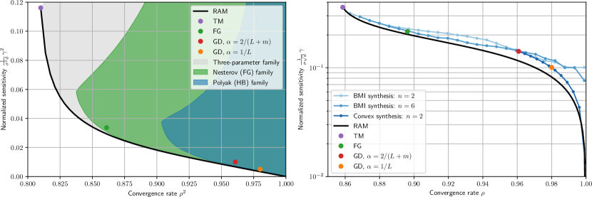
Figure 8: Left: Regions of the ($\rho$,$\gamma$) trade-off space for $F_{1,100}$ covered by the three-parameter family $(\alpha,\beta,\eta)$, the Nesterov (Fast Gradient) family $(\alpha,\beta,\beta)$, and the Polyak (Heavy Ball) family $(\alpha,\beta,0)$. The FG and HB families are not expressive enough to capture the whole trade-off space. Right: Comparison of RAM with the numerically synthesized algorithms (using a state dimension up to $n=6$) from [29] for $F_{1,50}$. RAM outperforms in spite of using only two states of memory. We plot $\log\gamma$ vs. $\rho$ to match [29, Fig. 6].

6.4 Simulation of a worst-case test function

We simulated various algorithms on Nesterov’s lower-bound function, which is a quadratic with a tridiagonal Hessian [35, §2.1.4]. We used $d=100$ with $m=1$ and $L=10$ and initialized each algorithm at zero. The results are reported in Fig. 9. We tested both a low noise ($\sigma=10^{-5}$, left column) and a higher noise ($\sigma=10^{-2}$, right column) regime. We recorded the mean and standard deviation of the error across $100$ trials for each algorithm (the trials differ only in the noise realization).

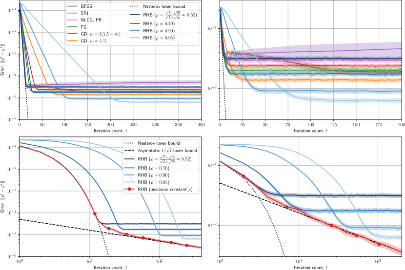
Figure 9: Simulations of various algorithms with low noise ($\sigma=10^{-5}$, left column) and higher noise ($\sigma=10^{-2}$, right column). Each algorithm was simulated on Nesterov’s lower-bound quadratic function, with $m=1$, $L=10$, and dimension $d=100$. Shaded regions indicate $\pm 1$ standard deviations about the mean across $100$ trials (different noise realizations). Different tunings of our proposed Robust Heavy Ball (RHB) from 9 yield an optimal trade-off between convergence rate and steady-state error (sensitivity to noise). Bottom row: the red curve shows RHB with piecewise constant $\rho$, where the red dots indicate switch points.

Fig. 9 shows that our Robust Heavy Ball (RHB) method from 9 trades off convergence rate (the slope of the initial decrease) with sensitivity to noise (the value of the steady-state error). and compares favorably to a variety of other methods. The other methods we tested (first row of Fig. 9) are generally suboptimal compared to RHB, in the sense that there is some choice of tuning parameter $\rho$ such that RHB is both faster and has smaller steady-state error.

In addition to gradient descent (GD) and Nesterov’s method (FG), we tested Nonlinear Conjugate Gradient (NLCG) with Polak-Ribière (PR) update scheme. NLCG performs similarly to RHB with the most aggressive tuning, which is equivalent to the Heavy Ball method. We also tested the popular quasi-Newton methods [36] Broyden–Fletcher–Goldfarb–Shanno (BFGS) and Symmetric Rank-One (SR1), which performed strictly worse than RHB. Both NLCG and BFGS involve line searches. That is, given a current point $y\in\mathbb{R}^{d}$ and search direction $s\in\mathbb{R}^{d}$, we must find $\alpha\in\mathbb{R}$ such that we minimize $f(y+\alpha s)$. In practice, inexact line searches are performed at each timestep, with a stopping criterion such as the Wolfe conditions. To show these algorithms in the most charitable possible light, we used exact line searches but substituted the noisy gradient oracle. Specifically, with $f(y)=\frac{1}{2}(y-y^{\star})^{\mathsf{T}}Q(y-y^{\star})$, the optimal stepsize is $\alpha^{\star}=-(s^{\mathsf{T}}\nabla\!f(y))/(s^{\mathsf{T}}Qs)$. We used this formula, but replaced $\nabla\!f(y)$ by the noisy gradient $\nabla\!f(y)+w$. In other words, we assumed exact knowledge of $Q$ but not of $y^{\star}$.

In the second row of Fig. 9, we duplicate the settings of the first row, except plot iterations on a log scale as in Fig. 1. Here, we also show a hand-tuned version of RHB with piecewise constant parameter $\rho$. Every time $\rho$ is changed, we re-initialize the algorithm by setting $x_{t-1}=x_{t}$ When the error is large compared to the noise level, the algorithm matches Nesterov’s lower bound (14), which is the lower bound associated with this particular function that holds for any algorithm when $t<d$. When the error is small compared to the noise level, the algorithm matches the asymptotic lower bound (slope of $-1/2$) described in Sections 1.2 and 6.2.

7 Concluding remarks

For each of the function classes $Q_{m,L}$, $F_{m,L}$, and $S_{m,L}$, we have provided (i) efficient methods for computing the convergence rate $\rho$ and noise sensitivity $\gamma$ for a broad class of first-order methods, and (ii) Near-Pareto-optimal first-order algorithm designs, each with a single tunable parameter that directly trades off $\rho$ versus $\gamma$.

An interesting future direction is to explore adaptive versions of these algorithms, for example where the parameter $\rho$ is increased over time. We showed in Fig. 9 that a hand-tuned piecewise constant version of RHB can match both Nesterov’s lower bound and the gradient lower bound in the asymptotic regime, so more sophisticated adaptive schemes such as those described in Section 1.2 might also work.

It may also be possible to adjust parameters continually (rather than in a piecewise fashion), but proving the convergence of adaptive algorithms is generally more challenging. For example, the well-known ADMM algorithm is often tuned adaptively to improve transient performance, even when convergence guarantees only hold for fixed parameters [7, §3.4.1.]. Nevertheless, LMI-based approaches have been successfully used to prove convergence of algorithms with time-varying parameters [21, 18].

Another interesting open question is whether our analysis is tight. For the function class $F_{m,L}$, our bounds depend on the lifting dimension $\ell$, and it is an open question how large $\ell$ needs to be in order to obtain tight bounds on $\rho$ and $\gamma$.

8 Acknowledgments

We would like to thank Jason Lee for his helpful comments and insights regarding the statistical aspects of this work. L. Lessard is partially supported by the National Science Foundation under Grants No. 1750162 and 1936648.

Appendix A Proofs

A.1 Proof of 8 ($Q_{m,L}$ analysis, reduced)

Convergence rate.

Given a polynomial $z^{2}+a_{1}z+a_{0}$ with real coefficients, a necessary and sufficient condition for its roots to lie inside the unit circle is given by the Jury test [17, §4.5]. In this case, the Jury test amounts to the inequalities

$$1+a_{1}+a_{0} >0, 1-a_{1}+a_{0} >0, -1<a_{0} <1.$$

Substituting the algorithm form (10) into 7, we obtain

$$\rho(\mathcal{A},Q_{m,L})=\sup_{q\in[m,L]}\underbrace{\rho\left(\begin{bmatrix}\beta+1-\alpha(\eta+1)q&-\beta+\alpha\eta q\\ 1&0\end{bmatrix}\right)}_{\phi(q)}$$ (37)

We will prove that the function inside the supremum, $\phi(q)$, is quasiconvex [8, §3.4]. The characteristic polynomial associated with the matrix in (37) is $\chi(z)=z^{2}+(\alpha(\eta+1)q-\beta-1)z+(\beta-\alpha\eta q)$. Applying the Jury test to $\chi(\rho z)$, we find that $\phi(q)<\rho$ if and only if

$$(1-\rho)(\beta-\rho)+\alpha(\eta\rho-\eta+\rho)q >0$$ (38a)

$$(1+\rho)(\beta+\rho)-\alpha(\eta\rho+\eta+\rho)q >0$$ (38b)

$$\rho^{2}+\beta-\alpha\eta q >0$$ (38c)

$$\rho^{2}-\beta+\alpha\eta q >0$$ (38d)

The inequalities (38) are linear in $q$, so the sublevel sets $\left\{q\;|\;\phi(q)<\rho\right\}$ are open intervals, which are convex. Therefore, $\phi$ is quasiconvex and attains its supremum over $q\in[m,L]$ at one of the endpoints $q=m$ or $q=L$. The explicit formula for $\phi(q)$ can be found by applying the quadratic formula to find the roots of $\chi(z)$.

Sensitivity.

Substituting the algorithm form (10) into 7, we can explicitly solve the linear equation for $P_{q}$ in (16) and substitute it into $\psi(q)=B^{\mathsf{T}}P_{q}B$ to obtain

$$\psi(q)=\frac{\alpha(1+\beta+(1+2\eta)\alpha\eta q)\sigma^{2}}{q(1-\beta+\alpha\eta q)(2+2\beta-(1+2\eta)\alpha q)}$$

When $\rho=1$, the Jury conditions (38) reduce to:

$$\alpha q >0$$ (39a)

$$2\beta+2-\alpha(2\eta+1)q >0$$ (39b)

$$1+\beta-\alpha\eta q >0$$ (39c)

$$1-\beta+\alpha\eta q >0.$$ (39d)

We will prove that when $\rho(\mathcal{A},Q_{m,L})<1$, $\psi(q)$ is a positive and convex function of $q$. Evaluating $\psi(q)$ and $\psi^{\prime\prime}(q)$ and performing algebraic manipulations, we obtain:

$$\psi(q) =\frac{\alpha^{2}(2\eta+1)^{2}}{2(1-\beta+\alpha\eta q)(2\beta+2-\alpha(2\eta+1)q)}+\frac{\alpha^{2}}{2\alpha q(\alpha\eta q-\beta+1)}$$ (40a)

$$\psi^{\prime\prime}(q) =\frac{\alpha^{4}(2\eta+1)^{2}\Bigl{(}3(2\alpha\eta(2\eta+1)q-4\beta\eta-\beta+1)^{2}+(4\eta-\beta+1)^{2}\Bigr{)}}{4(1-\beta+\alpha\eta q)^{3}(2\beta+2-\alpha(2\eta+1)q)^{3}}$$

$$\hskip 170.71652pt+\frac{\alpha q\Bigl{(}3\bigl{(}2\alpha\eta q+1-\beta\bigr{)}^{2}+\bigl{(}1-\beta\bigr{)}^{2}\Bigr{)}}{4q^{4}(\alpha\eta q-\beta+1)^{3}}$$ (40b)

In the form (40), it is clear that whenever $\rho(\mathcal{A},Q_{m,L})<1$ (i.e., when (39) holds) we have $\psi(q)>0$ and $\psi^{\prime\prime}(q)>0$. So the quantity under the square root in (16) is always positive, and $\psi(q)$ is convex, so it attains its supremum over $q\in[m,L]$ at one of the endpoints $q=m$ or $q=L$.

A.2 Proof of 9 (Robust Heavy Ball, RHB)

Applying 8, substitute $\alpha=\frac{1}{m}(1-\rho)^{2}$, $\beta=\rho^{2}$, and $\eta=0$ into (15) to obtain

$$\Delta=-(1-\rho)^{4}\left(\frac{q}{m}-1\right)\biggl{(}\biggl{(}\frac{1+\rho}{1-\rho}\biggr{)}^{2}-\frac{q}{m}\biggr{)}.$$

Rearranging the inequalities $m\leq q\leq L$ and $\frac{\sqrt{L}-\sqrt{m}}{\sqrt{L}+\sqrt{m}}\leq\rho<1$ yields $1\leq\frac{q}{m}\leq\frac{L}{m}\leq\bigl{(}\frac{1+\rho}{1-\rho}\bigr{)}^{2}<\infty$. Thus, we conclude that $\Delta\leq 0$ and we have $\rho(\mathcal{A},Q_{m,L})=\sqrt{\beta}=\rho$, as required.

Substituting $\alpha=\frac{1}{m}(1-\rho)^{2}$, $\beta=\rho^{2}$, and $\eta=0$ into (16), the expression under the square root is $h(q)\mathrel{\mathchoice{\vbox{\hbox{$\displaystyle:$}}}{\vbox{\hbox{$\textstyle:$}}}{\vbox{\hbox{$\scriptstyle:$}}}{\vbox{\hbox{$\scriptscriptstyle:$}}}{=}}\frac{\sigma^{2}d(1-\rho)\left(1+\rho^{2}\right)}{q(1+\rho)\left(2m-q+2q\rho+2m\rho^{2}-q\rho^{2}\right)}$, which is maximized when $q=m$. To see why, observe that:

$$h(m)-h(L)=\frac{\sigma^{2}d(1-\rho)\left(\rho^{2}+1\right)\left(\frac{L}{m}-1\right)\left(\bigl{(}\frac{1+\rho}{1-\rho}\bigr{)}^{2}-\frac{L}{m}\right)}{Lm(\rho+1)^{3}\left(1+\bigl{(}\frac{1+\rho}{1-\rho}\bigr{)}^{2}-\frac{L}{m}\right)}\geq 0$$

If follows that $\gamma(\mathcal{A},Q_{m,L},\sigma^{2})=\sqrt{h(m)}=\frac{\sigma\sqrt{d}}{m}\sqrt{\frac{1-\rho^{4}}{(1+\rho)^{4}}}$ as required.   

A.3 Proof of 11 ($S_{m,L}$ analysis)

Consider any trajectory $(\tilde{\xi}^{t},\tilde{u}^{t},\tilde{y}^{t},w^{t})_{t\geq 0}$ of the dynamics (6) with $w^{t}=0$, where we have shifted the fixed point as per 3 and 2. Multiply the LMI (18) on the left and right by $\begin{bmatrix}(\tilde{\xi}^{t})^{\mathsf{T}}&(\tilde{u}^{t})^{\mathsf{T}}\end{bmatrix}$ and its transpose, respectively, and obtain

$$(\tilde{\xi}^{t+1})^{\mathsf{T}}P\tilde{\xi}^{t+1}-\rho^{2}(\tilde{\xi}^{t})^{\mathsf{T}}P\tilde{\xi}^{t}+\lambda\begin{bmatrix}\tilde{y}^{t}\\ \tilde{u}^{t}\end{bmatrix}^{\mathsf{T}}\begin{bmatrix}-2mL&m+L\\ m+L&-2\end{bmatrix}\begin{bmatrix}\tilde{y}^{t}\\ \tilde{u}^{t}\end{bmatrix}\preceq 0$$

Taking the trace of both sides, defining $V(\xi)\mathrel{\mathchoice{\vbox{\hbox{$\displaystyle:$}}}{\vbox{\hbox{$\textstyle:$}}}{\vbox{\hbox{$\scriptstyle:$}}}{\vbox{\hbox{$\scriptscriptstyle:$}}}{=}}\operatorname{\mathrm{tr}}\left(\xi^{\mathsf{T}}P\xi\right)$, and applying (17), we conclude that $V(\xi^{t+1})\leq\rho^{2}V(\xi^{t})$. Moreover, since $P\succeq C^{\mathsf{T}}C$, we have $V(\xi^{t})\geq\lVert{y^{t}-y^{\star}}\rVert^{2}$. In other words, $V$ satisfies the lower bound condition and decrease condition from Section 4.1; it is a Lyapunov function. Specifically,

$$\lVert{y^{t}-y^{\star}}\rVert^{2}=\lVert{C\tilde{\xi}^{t}}\rVert^{2}\leq V(\tilde{\xi}^{t})\leq\rho^{2}V(\tilde{\xi}^{t-1})\leq\dots\leq\rho^{2t}V(\tilde{\xi}^{0})\leq\lambda_{\text{max}}(P)\rho^{2t}\lVert{\tilde{\xi}^{0}}\rVert^{2}.$$

Consequently, $\lVert{y^{t}-y^{\star}}\rVert\leq\sqrt{\lambda_{\text{max}}(P)}\rho^{t}\lVert{\xi^{0}-\xi^{\star}}\rVert$ and therefore $\rho(\mathcal{A},S_{m,L})\leq\rho$.

For the second part, do not restrict $w^{t}=0$, multiply the LMI (19) on the left and right by $\begin{bmatrix}(\tilde{\xi}^{t})^{\mathsf{T}}&(\tilde{u}^{t})^{\mathsf{T}}\end{bmatrix}$ and its transpose, respectively, and obtain

$$(\tilde{\xi}^{t+1}-Bw^{t})^{\mathsf{T}}P(\tilde{\xi}^{t+1}-Bw^{t})-(\tilde{\xi}^{t})^{\mathsf{T}}P\tilde{\xi}^{t}+\lambda\begin{bmatrix}\tilde{y}^{t}\\ \tilde{u}^{t}\end{bmatrix}^{\mathsf{T}}\begin{bmatrix}-2mL&m+L\\ m+L&-2\end{bmatrix}\begin{bmatrix}\tilde{y}^{t}\\ \tilde{u}^{t}\end{bmatrix}+\lVert{\tilde{y}^{t}}\rVert^{2}\preceq 0$$

Taking the trace of both sides, defining $\hat{V}(\xi)\mathrel{\mathchoice{\vbox{\hbox{$\displaystyle:$}}}{\vbox{\hbox{$\textstyle:$}}}{\vbox{\hbox{$\scriptstyle:$}}}{\vbox{\hbox{$\scriptscriptstyle:$}}}{=}}\operatorname{\mathrm{tr}}\left(\xi^{\mathsf{T}}P\xi\right)$, and applying (17), we obtain

$$\hat{V}(\tilde{\xi}^{t+1})-\hat{V}(\tilde{\xi}^{t})-2\operatorname{\mathrm{tr}}\bigl{(}A\tilde{\xi}^{t}+B\tilde{u}^{t}\bigr{)}^{\mathsf{T}}PBw^{t}+\lVert{\tilde{y}^{t}}\rVert^{2}\leq\operatorname{\mathrm{tr}}\bigl{(}(w^{t})^{\mathsf{T}}B^{\mathsf{T}}PBw^{t}\bigr{)}$$

Taking expectations of both sides with respect to $w\sim\mathbb{P}$, the third term vanishes because of the independence-across-time assumption and we may bound the right-hand side using the covariance bound $\sigma^{2}I_{d}$. $B\in\mathbb{R}^{n\times 1}$ so $B^{\mathsf{T}}PB$ is a scalar, and we obtain

$$\operatorname{\mathbb{E}}\hat{V}(\xi^{t+1})-\operatorname{\mathbb{E}}\hat{V}(\xi^{t})+\operatorname{\mathbb{E}}\lVert{\tilde{y}^{t}}\rVert^{2}\leq\sigma^{2}d\,(B^{\mathsf{T}}PB)$$

In addition, $P\succeq 0$ implies that $\operatorname{\mathbb{E}}\hat{V}(\xi^{t})\geq 0$. Thus $\hat{V}$ satisfies the lower bound condition and the increment condition from Section 4.1. Specifically, if we average over $t=0,1,\dots,T-1$, we obtain

$$0\leq\frac{1}{T}\operatorname{\mathbb{E}}\hat{V}(\xi^{T})\leq\frac{1}{T}\operatorname{\mathbb{E}}\hat{V}(\xi^{0})+\operatorname{\mathbb{E}}\sum_{t=0}^{T-1}\lVert{\tilde{y}^{t}}\rVert^{2}\leq\sigma^{2}d\,(B^{\mathsf{T}}PB).$$

Consequently, $\gamma(\mathcal{A},S_{m,L},\Sigma)\leq\sqrt{\sigma^{2}d\,(B^{\mathsf{T}}PB)}$, as required.   

A.4 Proof of 12

Assume (18) holds; multiply by $\left[\begin{smallmatrix}I\\ qC\end{smallmatrix}\right]^{\mathsf{T}}$ and $\left[\begin{smallmatrix}I\\ qC\end{smallmatrix}\right]$ on the left and right, respectively, and obtain:

$$(A+qBC)^{\mathsf{T}}P(A+qBC)-\rho^{2}P+2\lambda(L-q)(q-m)C^{\mathsf{T}}C\preceq 0$$

So whenever $q\in[m,L]$, we have $(A+qBC)^{\mathsf{T}}P(A+qBC)\preceq\rho^{2}P$. Let $\mu$ be an eigenvalue of $(A+qBC)$ with eigenvector $v$. Multiply by $v^{*}$ and $v$ on the left and right, respectively, to obtain: $\left(\rho^{2}-|\mu|^{2}\right)(v^{*}Pv)\geq 0$. Since $P\succeq I_{n}$, we have $v^{*}Pv>0$ and so $|\mu|\leq\rho$, and $\rho(A+qBC)\leq\rho$.

Now assume (19) holds. Proceeding in the same fashion as before, we deduce that when $q\in[m,L]$ and $\rho(\mathcal{A},Q_{m,L})<1$, we have

$$(A+qBC)^{\mathsf{T}}P(A+qBC)-P+C^{\mathsf{T}}C\preceq 0\quad\text{and}\quad\gamma^{2}\leq\sigma^{2}d(B^{\mathsf{T}}PB).$$

In an effort to find the least upper bound on $\gamma(\mathcal{A},S_{m,L},\sigma^{2})$, we consider the optimization problem:

$$p^{\star}=\underset{P\succeq 0}{\text{minimize}}\quad B^{\mathsf{T}}PB$$

subject to $$(A+qBC)^{\mathsf{T}}P(A+qBC)-P+C^{\mathsf{T}}C\preceq 0.$$

An upper bound to $p^{\star}$ can be found by replacing the semidefinite constraint by an equality. This is a standard Lyapunov equation and since $\rho(A+qBC)<1$, its solution has the explicit form $P=\sum_{k=0}^{\infty}{(A+qBC)^{\mathsf{T}}}^{k}C^{\mathsf{T}}C(A+qBC)^{k}$, and therefore $p^{\star}\leq B^{\mathsf{T}}PB=\sum_{k=0}^{\infty}\left[C(A+qBC)^{k}B\right]^{2}$. A lower bound to $p^{\star}$ can be found via the dual, which is the optimization problem:

$$d^{\star}=\underset{Q\succeq 0}{\text{maximize}}\quad CQC^{\mathsf{T}}$$

subject to $$(A+qBC)Q(A+qBC)^{\mathsf{T}}-Q+BB^{\mathsf{T}}\succeq 0.$$

A lower bound to $d^{\star}$ can be found by replacing the semidefinite constraint by an equality. Then we have $Q=\sum_{k=0}^{\infty}{(A+qBC)}^{k}BB^{\mathsf{T}}{(A+qBC)^{\mathsf{T}}}^{k}$ and then $\sum_{k=0}^{\infty}\left[C(A+qBC)^{k}B\right]^{2}=CQC^{\mathsf{T}}\leq d^{\star}$. So by weak duality, we have

$$\sum_{k=0}^{\infty}\left[C(A+qBC)^{k}B\right]^{2}\leq d^{\star}\leq p^{\star}\leq\sum_{k=0}^{\infty}\left[C(A+qBC)^{k}B\right]^{2}.$$

It follows that $d^{\star}=p^{\star}$ and the optimal solution to the primal is achieved when the semidefinite constraint is at equality. In other words, we recover $(A+qBC)^{\mathsf{T}}P(A+qBC)-P+C^{\mathsf{T}}C=0$ as in 7.   

A.5 Proof of 13 (Gradient Descent, GD)

For the case of Gradient Descent, the algorithm parameters from (6) are given by $A=C=1$ and $B=-\alpha$. So the LMIs (18)–(19) become:

$$\begin{bmatrix}(1-\rho^{2})P_{1}-2mL\lambda_{1}&-\alpha P_{1}+(L+m)\lambda_{1}\\ -\alpha P_{1}+(L+m)\lambda_{1}&\alpha^{2}P_{1}-2\lambda_{1}\end{bmatrix}\preceq 0,\quad P_{1}\geq 1,\quad\lambda_{1}\geq 0,$$

$$\begin{bmatrix}1-2mL\lambda_{2}&-\alpha P_{2}+(L+m)\lambda_{2}\\ -\alpha P_{2}+(L+m)\lambda_{2}&\alpha^{2}P_{2}-2\lambda_{2}\end{bmatrix}\preceq 0,\quad P_{2}\geq 0,\quad\lambda_{2}\geq 0,\quad\gamma(\mathcal{A},S_{m,L},\sigma^{2})\leq\sigma\alpha\sqrt{dP_{2}}.$$

Where $P_{1}$ and $P_{2}$ are now scalars. Substituting $\alpha=\frac{1}{m}(1-\rho)$, we can satisfy these LMIs using $P_{1}=P_{2}=\frac{1}{1-\rho^{2}}$ and $\lambda_{1}=\lambda_{2}=\frac{\rho}{m(L-m)(\rho+1)}$. With this solution choice, the two large matrices are equal to one another and the LMIs simplify to

$$-\frac{L+m}{m(L-m)(1+\rho)}\left(\rho-\frac{L-m}{L+m}\right)\begin{bmatrix}m&-1\\ -1&\frac{1}{m}\end{bmatrix}\preceq 0,\qquad\frac{1}{1-\rho^{2}}\geq 0,\qquad\frac{\rho}{m(L-m)(\rho+1)}\geq 0.$$

and this is satisfied for all $\frac{L-m}{L+m}\leq\rho<1$. Therefore, $\rho(\mathcal{A},S_{m,L})\leq\rho$ and $\gamma(\mathcal{A},S_{m,L},\sigma^{2})\leq\sigma\alpha\sqrt{dP_{2}}=\frac{\sigma\sqrt{d}}{m}\sqrt{\frac{1-\rho}{1+\rho}}$. To show that these upper bounds are tight, we will find a matching lower bound by consider the particular function $f\in S_{m,L}$ defined by $f(y)=\tfrac{1}{2}m\lVert{y}\rVert^{2}$. Since $f\in Q_{m,m}$, we can find $\rho(\mathcal{A},f)$ and $\gamma(\mathcal{A},f,\sigma^{2})$ by applying 8 with $L=m$. This results in the matching lower bounds $\rho=\rho(\mathcal{A},f)\leq\rho(\mathcal{A},S_{m,L})$ and $\frac{\sigma\sqrt{d}}{m}\sqrt{\frac{1-\rho}{1+\rho}}=\gamma(\mathcal{A},f,\sigma^{2})\leq\gamma(\mathcal{A},S_{m,L},\sigma^{2})$.   

A.6 Proof of 14 (Robust Gradient Descent, RGD)

Define $X$ to be the left-hand side of (18),

$$X\mathrel{\mathchoice{\vbox{\hbox{$\displaystyle:$}}}{\vbox{\hbox{$\textstyle:$}}}{\vbox{\hbox{$\scriptstyle:$}}}{\vbox{\hbox{$\scriptscriptstyle:$}}}{=}}\begin{bmatrix}A&B\\ I&0\end{bmatrix}^{\mathsf{T}}\begin{bmatrix}P&0\\ 0&-\rho^{2}P\end{bmatrix}\begin{bmatrix}A&B\\ I&0\end{bmatrix}+\lambda\begin{bmatrix}C&0\\ 0&1\end{bmatrix}^{\mathsf{T}}\begin{bmatrix}-2mL&m+L\\ m+L&-2\end{bmatrix}\begin{bmatrix}C&0\\ 0&1\end{bmatrix},$$

and substitute $A,B,C$ as functions of $(\alpha,\beta,\eta)$ using (10), so we have $X\in\mathbb{R}^{3\times 3}$. A feasible solution to this LMI is given by $\lambda=1$ and $P=\left[\begin{smallmatrix}p_{11}&p_{12}\\ p_{12}&p_{22}\end{smallmatrix}\right]$, where

$$p_{11} =\tfrac{-\alpha L(\rho-1)\left(\alpha m+\rho^{2}-1\right)-\alpha^{2}m^{2}(\rho+1)+\alpha m(\rho+1)(\rho-1)^{2}+2\rho(\rho-1)^{4}}{\alpha^{2}(\rho-1)\rho\left(\alpha m(\rho+1)+(\rho-1)^{3}\right)},$$

$$p_{12} =\tfrac{\alpha L(\rho-1)\left(3\alpha m-\rho^{2}+4\rho-3\right)+\alpha^{2}m^{2}(\rho+1)-\alpha m(3\rho-1)(\rho-1)^{2}-2(\rho-1)^{4}}{\alpha^{2}(\rho-1)\left(\alpha m(\rho+1)+(\rho-1)^{3}\right)},$$

$$p_{22} =\tfrac{\alpha L\left(-2\alpha^{2}m^{2}-\alpha m\left(\rho^{2}+3\rho-4\right)+(\rho-1)^{2}\left(\rho^{2}-\rho-2\right)\right)+\alpha^{2}m^{2}\left(\rho^{2}-5\rho+2\right)+\alpha m\left(\rho^{2}+5\rho-4\right)(\rho-1)^{2}+2(\rho-1)^{4}}{\alpha^{2}(\rho-1)\left(\alpha m(\rho+1)+(\rho-1)^{3}\right)}.$$

Using Mathematica [43], it is straightforward to verify that this choice satisfies $P\succ 0$ and $X\preceq 0$ for all choices of $(m,L,\rho,\alpha)$ satisfying $0<m\leq L$, $\frac{L-m}{L+m}<\rho<1$, and $\frac{(1-\rho)^{2}}{m}<\alpha<\frac{1-\rho^{2}}{m}$. Therefore, there exists a positive rescaling of $(P,\lambda)$ that satisfies the original requirement $P\succeq I_{n}$. So far, we have shown that $\rho(\mathcal{A},S_{m,L})\leq\rho$. To prove equality, we proceed as in the proof of 13. Again considering the function $f(y)=\tfrac{1}{2}m\lVert{y}\rVert^{2}$ and substituting the algorithm parameters from 14, the algorithm dynamics become

$$\xi^{t+1}=(A+mBC)\xi^{t}=\begin{bmatrix}\frac{1-\rho^{2}-\alpha m}{1-\rho}&-\frac{\rho(1-\rho-\alpha m)}{1-\rho}\\ 1&0\\ \end{bmatrix}\xi^{t}.$$

The eigenvalues of this matrix are $\rho$ and $\frac{1-\rho-\alpha m}{1-\rho}$. We see that $-\rho\leq\frac{1-\rho-\alpha m}{1-\rho}\leq\rho$ precisely when $\frac{(1-\rho)^{2}}{m}\leq\alpha\leq\frac{1-\rho^{2}}{m}$, and so $\rho=\rho(\mathcal{A},f)\leq\rho(\mathcal{A},S_{m,L})$, as required.

To prove the second part of the theorem, we work with the $\gamma$-LMI (19). At optimality, the LMI is rank-1. Equivalently, all $2\times 2$ minors of the LMI vanish. Also, the objective of the optimization is $\gamma^{2}=\alpha^{2}P_{11}$. Eliminating $P$ from these equations yields a polynomial equation $g(\alpha,\beta,\eta,m,L,\gamma,\lambda)=0$. Since we are minimizing $\gamma$ subject to $g=0$, the KKT conditions imply that $\frac{\mathrm{d}g}{\mathrm{d}\lambda}=0$. Since $g$ and its derivative are both zero, equivalently, the discriminant of $g$ with respect to $\lambda$ is zero. Now substitute the expressions for $\beta$ and $\eta$ from the theorem statement to obtain an equation of the form $\hat{J}(\alpha,\rho,\gamma,m,L)=0$. We would like to show that along solutions of $\hat{J}=0$, when $m,L,\rho$ are held fixed, $\gamma$ is a decreasing function of $\alpha$ near the initial point $\alpha=\frac{1}{m}(1-\rho)^{2}$ and $\gamma=\frac{\sigma\sqrt{d}}{m}\sqrt{\frac{1-\rho}{1+\rho}}$, which corresponds to GD. Computing total derivatives, we find

$$\frac{\mathrm{d}\gamma}{\mathrm{d}\alpha}=-\frac{\hat{J}_{\alpha}}{\hat{J}_{\gamma}}\quad\text{and}\quad\frac{\mathrm{d}^{2}\gamma}{\mathrm{d}\alpha^{2}}=-\frac{\hat{J}_{\alpha\alpha}\hat{J}_{\gamma}^{2}-2\hat{J}_{\alpha\gamma}\hat{J}_{\alpha}\hat{J}_{\gamma}+\hat{J}_{\gamma\gamma}\hat{J}_{\alpha}^{2}}{\hat{J}_{\gamma}^{3}},$$

where subscripts indicate partial derivatives. Evaluating at the initial point, we obtain

$$\frac{\mathrm{d}\gamma}{\mathrm{d}\alpha}=0,\qquad\frac{\mathrm{d}^{2}\gamma}{\mathrm{d}\alpha^{2}}=-\frac{\sigma\sqrt{d}\,m\,\frac{L+m}{L-m}\,(\rho-\frac{L-m}{L+m})}{\rho(1-\rho)^{7/2}(1+\rho)^{3/2}}<0.$$

Therefore, $\gamma$ is a decreasing function of $\alpha$ in a neighborhood of $\alpha=\frac{1}{m}(1-\rho)^{2}$, as required.   

A.7 Proof of 17

For each $i\in I$, define the vectors $\tilde{y}_{i}\mathrel{\mathchoice{\vbox{\hbox{$\displaystyle:$}}}{\vbox{\hbox{$\textstyle:$}}}{\vbox{\hbox{$\scriptstyle:$}}}{\vbox{\hbox{$\scriptscriptstyle:$}}}{=}}\mathsf{e}_{i}^{\mathsf{T}}\bm{y}^{t}$ and $\tilde{u}_{i}\mathrel{\mathchoice{\vbox{\hbox{$\displaystyle:$}}}{\vbox{\hbox{$\textstyle:$}}}{\vbox{\hbox{$\scriptstyle:$}}}{\vbox{\hbox{$\scriptscriptstyle:$}}}{=}}\mathsf{e}_{i}^{\mathsf{T}}\bm{u}^{t}$ and $\tilde{f}_{i}\mathrel{\mathchoice{\vbox{\hbox{$\displaystyle:$}}}{\vbox{\hbox{$\textstyle:$}}}{\vbox{\hbox{$\scriptstyle:$}}}{\vbox{\hbox{$\scriptscriptstyle:$}}}{=}}\mathsf{e}_{i}^{\mathsf{T}}\bm{f}^{t}$. By definition, the points $(\tilde{y}_{i},\tilde{u}_{i},\tilde{f}_{i})$ are interpolated by the function $f\in F_{m,L}$, so by 16 the interpolation conditions (20) are satisfied. The proof is then completed by noting that the inequality (29) can be expanded as

$$\sum_{i,j\in I}\Lambda_{ij}\Bigl{(}-mL\|\tilde{y}_{i}-\tilde{y}_{j}\|^{2}+2\,(\tilde{y}_{i}-\tilde{y}_{j})(m\tilde{u}_{i}-L\tilde{u}_{j})^{\mathsf{T}}-\|\tilde{u}_{i}-\tilde{u}_{j}\|^{2}+2(L-m)(\tilde{f}_{i}-\tilde{f}_{j})\Bigr{)}\geq 0,$$

which is a weighted combination of the interpolation conditions, where the interpolation condition between index $i$ and $j$ is scaled by the nonnegative quantity $2\,(L-m)\Lambda_{ij}\geq 0$.

A.8 Proof of 18 ($F_{m,L}$ analysis)

Consider any trajectory of the dynamics (6) with $w^{t}=0$, and form the augmented vectors and state as described in Section 5.1. Multiply the LMIs (32a) and (32c) on the right and left by $(\bm{x}_{r}^{t},\tilde{u}^{t})\in\mathbb{R}^{n+\ell+1}$ and its transpose, respectively, and take the trace. Also, take the inner product of (32b) and (32d) with $\bm{f}^{t}$, which is valid because $\bm{f}^{t}$ is elementwise nonnegative. The resulting inequalities are:

$$\operatorname{\mathrm{tr}}\,(\bm{x}_{r}^{t+1})^{\mathsf{T}}P\bm{x}_{r}^{t+1}-\rho^{2}\operatorname{\mathrm{tr}}\,(\bm{x}_{r}^{t})^{\mathsf{T}}P\bm{x}_{r}^{t}+\operatorname{\mathrm{tr}}\begin{bmatrix}\bm{y}^{t}\\ \bm{u}^{t}\end{bmatrix}^{\mathsf{T}}\Pi(\Lambda_{1})\begin{bmatrix}\bm{y}^{t}\\ \bm{u}^{t}\end{bmatrix} \leq 0$$ (41a)

$$p^{\mathsf{T}}(Z_{+}-\rho^{2}Z)\bm{f}^{t}+\pi(\Lambda_{1})^{\mathsf{T}}\bm{f}^{t} \leq 0$$ (41b)

$$\|\tilde{\xi}^{t}\|^{2}-\operatorname{\mathrm{tr}}\,(\bm{x}_{r}^{t})^{\mathsf{T}}P\bm{x}_{r}^{t}+\operatorname{\mathrm{tr}}\begin{bmatrix}\bm{y}^{t}\\ \bm{u}^{t}\end{bmatrix}^{\mathsf{T}}\Pi(\Lambda_{1})\begin{bmatrix}\bm{y}^{t}\\ \bm{u}^{t}\end{bmatrix} \leq 0$$ (41c)

$$-p^{\mathsf{T}}Z\bm{f}^{t}+\pi(\Lambda_{2})^{\mathsf{T}}\bm{f}^{t} \leq 0$$ (41d)

Summing (41a)$+$(41b) and (41c)$+$(41d) and applying (29), we recover the lower bound and exponential decrease properties

$$V(\bm{x}_{r}^{t+1},\bm{f}^{t+1})\leq\rho^{2}\,V(\bm{x}_{r}^{t},\bm{f}^{t})\qquad\text{and}\qquad V(\bm{x}_{r}^{t},\bm{f}^{t})\geq\|\tilde{\xi}^{t}\|^{2}$$

Applying the lower bound and then the exponential decrease bound recursively, we obtain

$$\|\xi^{t}-\xi^{\star}\|^{2}\leq V(\bm{x}_{r}^{t},\bm{f}^{t})\leq\ldots\leq\rho^{2t}\,V(\bm{x}_{r}^{0},\bm{f}^{0})$$

which implies that $\rho(\mathcal{A},F_{m,L})\leq\rho$.

For the second part of the proof, we do not restrict $w^{t}=0$, and perform similar operations to the inequalities (33) as in the first part, except that we multiply the linear matrix inequalities by $(\bm{x}^{t},\tilde{u}^{t})$ instead to obtain the inequalities

$$\operatorname{\mathrm{tr}}\,(\bm{x}^{t+1}-\bm{H}w^{t})^{\mathsf{T}}P(\bm{x}^{t+1}-\bm{H}w^{t})-\operatorname{\mathrm{tr}}\,(\bm{x}^{t})^{\mathsf{T}}P\bm{x}^{t}+\operatorname{\mathrm{tr}}\begin{bmatrix}\bm{y}^{t}\\ \bm{u}^{t}\end{bmatrix}^{\mathsf{T}}\Pi(\Lambda_{1})\begin{bmatrix}\bm{y}^{t}\\ \bm{u}^{t}\end{bmatrix}+\|\tilde{y}^{t}\|^{2} \leq 0$$ (42a)

$$p^{\mathsf{T}}(Z_{+}-Z)\bm{f}^{t}+\pi(\Lambda_{1})^{\mathsf{T}}\bm{f}^{t} \leq 0$$ (42b)

$$-\operatorname{\mathrm{tr}}\,(\bm{x}^{t})^{\mathsf{T}}P\bm{x}^{t}+\operatorname{\mathrm{tr}}\begin{bmatrix}\bm{y}^{t}\\ \bm{u}^{t}\end{bmatrix}^{\mathsf{T}}\Pi(\Lambda_{2})\begin{bmatrix}\bm{y}^{t}\\ \bm{u}^{t}\end{bmatrix} \leq 0$$ (42c)

$$-p^{\mathsf{T}}Z\bm{f}^{t}+\pi(\Lambda_{2})^{\mathsf{T}}\bm{f}^{t} \leq 0$$ (42d)

Summing (42a)$+$(42b) and (42c)$+$(42d) and applying (29), we obtain the inequalities

$$V(\bm{x}^{t+1},\bm{f}^{t+1})-V(\bm{x}^{t},\bm{f}^{t})+\|\tilde{y}^{t}\|^{2}-2\,\operatorname{\mathrm{tr}}\,(\bm{A}\bm{x}^{t}+\bm{B}\tilde{u}^{t})^{\mathsf{T}}P\bm{H}w^{t}-\operatorname{\mathrm{tr}}{w^{t}}^{\mathsf{T}}\bm{H}^{\mathsf{T}}P\bm{H}w^{t} \leq 0$$ (43a)

$$-V(\bm{x}^{t},\bm{f}^{t}) \leq 0$$ (43b)

Taking the expectation of both inequalities, the term $-2(\bm{A}\bm{x}^{t}+\bm{B}\tilde{u}^{t})^{\mathsf{T}}P\bm{H}w^{t}$ in the first inequality vanishes because $w^{t}$ is zero-mean and is independent of $\bm{x}^{t}$ and $u^{t}$, which only depend on $w^{t-1},w^{t-2},\dots$. Also, since $w^{t}$ has covariance bound $\sigma^{2}I$, we have $\operatorname{\mathrm{tr}}\operatorname{\mathbb{E}}\bigl{(}{w^{t}}^{\mathsf{T}}\bm{H}^{\mathsf{T}}P\bm{H}w^{t}\bigr{)}\leq\sigma^{2}d(\bm{H}^{\mathsf{T}}P\bm{H})$. Thus, the previous inequalities imply the decrease and nonnegativity conditions

$$\operatorname{\mathbb{E}}V(\bm{x}^{t+1},\bm{f}^{t+1})-\operatorname{\mathbb{E}}V(\bm{x}^{t},\bm{f}^{t})+\|\tilde{y}^{t}\|^{2}\leq\sigma^{2}d\,(\bm{H}^{\mathsf{T}}P\bm{H})\qquad\text{and}\qquad\operatorname{\mathbb{E}}V(\bm{x}^{t},\bm{f}^{t})\geq 0.$$

Summing the decrease condition over $t=0,\dots,T-1$, the sum telescopes and upon applying the nonnegativity condition, we obtain

$$0\leq\operatorname{\mathbb{E}}V(\bm{x}^{T},\bm{f}^{T})\leq\operatorname{\mathbb{E}}V(\bm{x}^{0},\bm{f}^{0})-\operatorname{\mathbb{E}}\sum_{k=0}^{T-1}\|\tilde{y}^{t}\|^{2}+T\sigma^{2}d\,(\bm{H}^{\mathsf{T}}P\bm{H}).$$

Rearranging, dividing by $T$, and letting $T\to\infty$, we obtain

$$\limsup_{T\to\infty}\operatorname{\mathbb{E}}\frac{1}{T}\sum_{t=0}^{T-1}\|\tilde{y}^{t}\|^{2}\leq\sigma^{2}d\,(\bm{H}^{\mathsf{T}}P\bm{H})$$

which implies that $\gamma(\mathcal{A},F_{m,L},\sigma^{2})\leq\sqrt{\sigma^{2}d\,(\bm{H}^{\mathsf{T}}P\bm{H})}$.   

A.9 Proof of 21 (Robust Accelerated Method, RAM)

To prove that RAM converges with rate $\rho$ when there is no noise, we provide a feasible solution to the LMI (32) with lifting dimension $\ell=1$. In fact, our solution has the same structure as the weighted off-by-one IQC formulation in (34), where the positive definite matrix $Q\succ 0$ is given by

$$Q =\frac{m}{(3-\rho)(1-\rho)^{2}(1+\rho)^{3}\bigl{(}m-L\,(1-\rho)^{2}\bigr{)}}\begin{bmatrix}q_{11}&q_{12}&q_{13}\\ q_{12}&q_{22}&q_{23}\\ q_{13}&q_{23}&q_{33}\end{bmatrix},\quad\text{with}$$

$$q_{11} =\rho\,\bigl{(}2m^{2}(1-\rho)+2Lm\,(4+\rho-2\rho^{2}+\rho^{3})-L^{2}(1-\rho^{2})^{2}\bigr{)},$$

$$q_{12} =\rho\,\bigl{(}-2m^{2}(1-\rho)-2Lm\,(1+\rho)^{2}+L^{2}(4-\rho)(1-\rho^{2})^{2}\bigr{)},$$

$$q_{13} =(3-\rho)(1-\rho^{2})\bigl{(}-m\,(1+\rho^{2})+L\,(1+\rho-2\rho^{2}-\rho^{3}+\rho^{4})\bigr{)},$$

$$q_{22} =\rho\,\bigl{(}2m^{2}(1-\rho)-2Lm\,(2-3\rho-4\rho^{2}+\rho^{3})+L^{2}(2-4\rho+\rho^{2})(1-\rho^{2})^{2}\bigr{)},$$

$$q_{23} =\rho\,(3-\rho)(1-\rho^{2})\bigl{(}m\,(-1+2\rho+\rho^{2})-L\,(-1+\rho-\rho^{3}+\rho^{4})\bigr{)},$$

$$q_{33} =\rho\,(3-\rho)^{2}(1-\rho^{2})^{2}.$$

Using Mathematica [43], it is straightforward to verify that, for all parameters $0<m\leq L$ with $1-\sqrt{\frac{m}{L}}\leq\rho<1$, this is a feasible solution to a modified version of the LMI (32) in which the term $\bm{X}_{r}^{\mathsf{T}}\bm{X}_{r}$ is replaced by $\bm{X}_{r}^{\mathsf{T}}T^{\mathsf{T}}QT\bm{X}_{r}$, where

$$T=\begin{bmatrix}A&B\\ -LC&1\end{bmatrix}.$$

Since $T^{\mathsf{T}}QT$ is strictly positive definite, we have $\bm{X}_{r}^{\mathsf{T}}T^{\mathsf{T}}QT\bm{X}_{r}\succeq c\,\bm{X}_{r}^{\mathsf{T}}\bm{X}_{r}$, where $c>0$ is the minimum eigenvalue of $T^{\mathsf{T}}QT$. Therefore, scaling the entire solution by $1/c$ provides a feasible solution to the original LMI (32). 18 then implies that RAM has convergence rate at least $\rho$. To show that the convergence rate is exactly $\rho$, note that the spectral radius of $A+mBC$ is precisely $\rho$, which completes the proof.   

A.10 Proof of 23 (algorithm parameter restriction)

The Jury criterion for stability ($\rho<1$) is given in (39). Combining $\eqref{eb}+2\cdot\eqref{ed}$ together with (39a), we obtain: $0<\alpha q<4$. This must hold for all $q\in[m,L]$, so we conclude that $0<\alpha<\frac{4}{L}$. Combining (39c) and (39d), we obtain $-1+\alpha\eta q<\beta<1+\alpha\eta q$. This must hold for all $q\in[m,L]$. We consider two cases. When $\alpha\eta\geq 0$, the $\beta$ range reduces to $-1+L(\alpha\eta)<\beta<1+m(\alpha\eta)$ and consequently, $\alpha\eta<\frac{2}{L-m}$. When $\alpha\eta<0$, we instead obtain $-1+m(\alpha\eta)<\beta<1+L(\alpha\eta)$ and $\frac{-2}{L-m}<\alpha\eta$, thus completing the proof. Although these bounds are derived for the function class $Q_{m,L}$, the nestedness property $Q_{m,L}\subseteq F_{m,L}\subseteq S_{m,L}$ implies that these necessary conditions on $(\alpha,\beta,\eta)$ also hold for $F_{m,L}$ and $S_{m,L}$.   

Appendix B Numerical considerations for solving LMIs

This section explains the details of how we numerically solved the linear matrix inequalities in 11 and 18. We used the Julia programming language version 1.6 [6] along with the Convex.jl package version 0.14 [41] to model the optimization problems that were then solved using Mosek version 9.3 [3]. For RGD, we used Brent’s method in the Optim.jl package version 1.3 [30] to find the stepsize $\alpha$ that minimizes the sensitivity. All simulations and numerical experiments were conducted on a laptop computer with conventional hardware.

Solving LMIs for the class $S_{m,L}$.

Given an algorithm $(\alpha,\beta,\eta)$, each solve of (19) to find $\gamma$ took approximately 2 ms. Finding $\rho$ required multiple solves of (18) using a bisection search, which took approximately 44 ms (using a tolerance of $10^{-6}$). Therefore, each plot in Fig. 6 took roughly 7 hours to compute.

Solving LMIs for the class $F_{m,L}$.

Solving the LMIs in 18 first requires choosing a lifting dimension $\ell$. Increasing $\ell$ yields potentially tighter bounds on $\rho$ and $\gamma$, but at the expense of making the LMIs larger and more time-consuming to solve. We also found empirically that the $\gamma$ LMI (33), becomes poorly conditioned when $\ell$ is large or when $L/m$ is large. One way to improve the conditioning of the problem is via a similarity transform. For example, given any invertible matrix $T$, the LMI (33) used to compute $\gamma$ for the function class $F_{m,L}$ is feasible if and only if it is feasible under the transformation

$$(\bm{A},\bm{B},\bm{H},\bm{C},\bm{Y})\mapsto\biggl{(}T\bm{A}T^{-1},T\bm{B},T\bm{H},\bm{C}T^{-1},\bm{Y}\begin{bmatrix}T^{-1}&0\\ 0&1\end{bmatrix}\biggr{)},$$

which corresponds to transforming the lifted state as $\bm{x}^{t}\mapsto T\bm{x}^{t}$ and the solution transforms as $P\mapsto T^{-\mathsf{T}}PT^{-1}$ with $p$, $\Lambda_{1}$, $\Lambda_{2}$, and $\gamma$ unchanged. A similar transformation is also possible for computing $\rho$ via (32). Transforming the LMIs via an appropriately chosen $T$ can lead to improved conditioning and solver performance. As a heuristic, we used a transformation inspired by the balanced realization [45, §3.9]. In particular, we chose $T$ to be the transformation that balances the scaled system $(\theta^{-1}\bm{A},\theta^{-1}\begin{bmatrix}\bm{B}&\bm{H}\end{bmatrix},\theta^{-1}\bm{C})$, with $\theta\mathrel{\mathchoice{\vbox{\hbox{$\displaystyle:$}}}{\vbox{\hbox{$\textstyle:$}}}{\vbox{\hbox{$\scriptstyle:$}}}{\vbox{\hbox{$\scriptscriptstyle:$}}}{=}}1.1\cdot\rho(A)$.

To decide which lifting dimension to use, we performed pilot tests to observe how the $\rho$ and $\gamma$ bounds improved as $\ell$ was increased. In Table 3, we show some representative results, evaluating the performance of Nesterov’s Fast Gradient method with or without balancing. By definition, the bounds computed for $\rho$ and $\gamma$ should decrease (or stay the same) as we increase $\ell$. Any observed increases must be due to numerical solver error.

Table 3: Numerical values for Nesterov’s Fast Gradient method with standard tuning (see Table 1), with additional parameters $d=1$, $\sigma=1$, $m=1$, and $L=100$. Results obtained by computationally solving the LMIs from 18 using various values of the lifting dimension $\ell$. Numerical results are more reliable when balancing is used. Last column indicates the wall clock time for computing $\gamma$ with balancing (one LMI solve).

$\ell$	Rate $\rho$	Balanced $\rho$	Sensitivity $\gamma$	Balanced $\gamma$	Time (sec.)
1	0.9279379028	0.9279330969	0.2007657395	0.2007653112	0.0053
2	0.9279357392	0.9279330772	error	0.1859082519	0.0094
3	0.9279401124	0.9279330707	error	0.1837282849	0.0169
4	0.9279420203	0.9279330510	error	0.1835113705	0.0323
5	0.9279418892	0.9279330248	error	0.1834890908	0.0796
6	0.9279397845	0.9279329461	error	0.1834856744	0.1042
7	0.9279395616	0.9279328346	0.1834918867	0.1834813977	0.2000
8	0.9279494816	0.9279329133	0.1834920874	0.1834817113	0.3434
9	0.9279330379	0.9279327232	0.1834930651	0.1834868332	0.5947
10	0.9279350966	0.9279327756	error	0.1834840969	1.0601

In Table 3, we observe that $\rho$ reaches its minimal value at $\ell=1$, beyond which there is no improvement. Meanwhile, $\gamma$ continues to improve as $\ell$ increases. These observations regarding $\rho$ and $\gamma$ were robust across all algorithms we tested, so for all subsequent numerical simulations, including those of Fig. 6, we used $\ell=1$ for $\rho$ and $\ell=6$ for $\gamma$, both with balancing. In computing $\rho$, we used a bisection search with tolerance $10^{-6}$. Using these parameters, finding $\rho$ and $\gamma$ each took about 100 ms. Consequently each plot in Fig. 6 took roughly 30 hours to compute.

References

- [1] A. Agarwal, P. L. Bartlett, P. Ravikumar, and M. J. Wainwright. Information-theoretic lower bounds on the oracle complexity of stochastic convex optimization. IEEE Transactions on Information Theory, 58(5):3235–3249, 2012.
- [2] P. J. Antsaklis and A. N. Michel. Linear systems. Springer Science & Business Media, 2006.
- [3] M. ApS. The MOSEK optimization suite 9.2.49, 2021.
- [4] N. Aybat, A. Fallah, M. Gürbüzbalaban, and A. Ozdaglar. A universally optimal multistage accelerated stochastic gradient method. Advances in Neural Information Processing Systems, 32, 2019.
- [5] N. S. Aybat, A. Fallah, M. Gurbuzbalaban, and A. Ozdaglar. Robust accelerated gradient methods for smooth strongly convex functions. SIAM Journal on Optimization, 30(1):717–751, 2020.
- [6] J. Bezanson, A. Edelman, S. Karpinski, and V. B. Shah. Julia: A fresh approach to numerical computing. SIAM Review, 59(1):65–98, 2017.
- [7] S. Boyd, N. Parikh, and E. Chu. Distributed optimization and statistical learning via the alternating direction method of multipliers. Now Publishers Inc, 2011.
- [8] S. Boyd and L. Vandenberghe. Convex optimization. Cambridge University Press, 2004.
- [9] J. Chee and P. Toulis. Convergence diagnostics for stochastic gradient descent with constant learning rate. In A. Storkey and F. Perez-Cruz, editors, Proceedings of the Twenty-First International Conference on Artificial Intelligence and Statistics, volume 84 of Proceedings of Machine Learning Research, pages 1476–1485. PMLR, 09–11 Apr 2018.
- [10] S. Cyrus, B. Hu, B. V. Scoy, and L. Lessard. A robust accelerated optimization algorithm for strongly convex functions. In American Control Conference, pages 1376–1381, June 2018.
- [11] A. Defazio, F. Bach, and S. Lacoste-Julien. Saga: A fast incremental gradient method with support for non-strongly convex composite objectives. In Z. Ghahramani, M. Welling, C. Cortes, N. Lawrence, and K. Q. Weinberger, editors, Advances in Neural Information Processing Systems, volume 27. Curran Associates, Inc., 2014.
- [12] O. Devolder. Exactness, inexactness and stochasticity in first-order methods for large-scale convex optimization. PhD thesis, Université catholique de Louvain, ICTEAM and CORE, 2013.
- [13] O. Devolder, F. Glineur, and Y. Nesterov. First-order methods with inexact oracle: the strongly convex case. Core discussion paper; 2013/16, Université catholique de Louvain, May 2013.
- [14] O. Devolder, F. Glineur, and Y. Nesterov. Intermediate gradient methods for smooth convex problems with inexact oracle. Core discussion paper; 2013/17, Université catholique de Louvain, May 2013.
- [15] O. Devolder, F. Glineur, and Y. Nesterov. First-order methods of smooth convex optimization with inexact oracle. Mathematical Programming, 146(1-2):37–75, 2014.
- [16] Y. Drori and M. Teboulle. Performance of first-order methods for smooth convex minimization: a novel approach. Mathematical Programming, 145(1):451–482, 2014.
- [17] M. S. Fadali and A. Visioli. Digital control engineering: analysis and design. Academic Press, 2013.
- [18] M. Fazlyab, A. Ribeiro, M. Morari, and V. M. Preciado. Analysis of optimization algorithms via integral quadratic constraints: Nonstrongly convex problems. SIAM Journal on Optimization, 28(3):2654–2689, 2018.
- [19] R. Ge, S. M. Kakade, R. Kidambi, and P. Netrapalli. The step decay schedule: A near optimal, geometrically decaying learning rate procedure for least squares. In H. Wallach, H. Larochelle, A. Beygelzimer, F. d'Alché-Buc, E. Fox, and R. Garnett, editors, Advances in Neural Information Processing Systems, volume 32. Curran Associates, Inc., 2019.
- [20] E. Ghadimi, H. R. Feyzmahdavian, and M. Johansson. Global convergence of the heavy-ball method for convex optimization. In 2015 European Control Conference (ECC), pages 310–315, 2015.
- [21] B. Hu and L. Lessard. Dissipativity theory for Nesterov’s accelerated method. In International Conference on Machine Learning, pages 1549–1557, Aug. 2017.
- [22] B. Hu, P. Seiler, and L. Lessard. Analysis of biased stochastic gradient descent using sequential semidefinite programs. Mathematical Programming, 187(0):383–408, Mar. 2020.
- [23] P. Jain, S. M. Kakade, R. Kidambi, P. Netrapalli, and A. Sidford. Accelerating stochastic gradient descent for least squares regression. In S. Bubeck, V. Perchet, and P. Rigollet, editors, Proceedings of the 31st Conference On Learning Theory, volume 75 of Proceedings of Machine Learning Research, pages 545–604. PMLR, 06–09 Jul 2018.
- [24] R. Johnson and T. Zhang. Accelerating stochastic gradient descent using predictive variance reduction. In C. J. C. Burges, L. Bottou, M. Welling, Z. Ghahramani, and K. Q. Weinberger, editors, Advances in Neural Information Processing Systems, volume 26. Curran Associates, Inc., 2013.
- [25] M. J. Kochenderfer and T. A. Wheeler. Algorithms for optimization. MIT Press, 2019.
- [26] L. Lessard, B. Recht, and A. Packard. Analysis and design of optimization algorithms via integral quadratic constraints. SIAM Journal on Optimization, 26(1):57–95, 2016.
- [27] L. Lessard and P. Seiler. Direct synthesis of iterative algorithms with bounds on achievable worst-case convergence rate. In American Control Conference, July 2020.
- [28] A. Megretski and A. Rantzer. System analysis via integral quadratic constraints. IEEE Transactions on Automatic Control, 42(6):819–830, 1997.
- [29] S. Michalowsky, C. Scherer, and C. Ebenbauer. Robust and structure exploiting optimisation algorithms: an integral quadratic constraint approach. International Journal of Control, 0(0):1–24, 2020.
- [30] P. K. Mogensen and A. N. Riseth. Optim: A mathematical optimization package for Julia. Journal of Open Source Software, 3(24):615, 2018.
- [31] H. Mohammadi, M. Razaviyayn, and M. R. Jovanović. Robustness of accelerated first-order algorithms for strongly convex optimization problems. IEEE Transactions on Automatic Control, 66(6):2480–2495, 2021.
- [32] E. Moulines and F. Bach. Non-asymptotic analysis of stochastic approximation algorithms for machine learning. In Advances in Neural Information Processing Systems, volume 24. Curran Associates, Inc., 2011.
- [33] I. Necoara, Y. Nesterov, and F. Glineur. Linear convergence of first order methods for non-strongly convex optimization. Mathematical Programming, 175(1-2):69–107, 2019.
- [34] A. S. Nemirovsky and D. B. Yudin. Problem complexity and method efficiency in optimization. Wiley-Interscience, 1983.
- [35] Y. Nesterov. Lectures on convex optimization, volume 137. Springer, 2018.
- [36] J. Nocedal and S. Wright. Numerical optimization. Springer Science & Business Media, 2006.
- [37] B. T. Polyak. Introduction to optimization. Translations series in mathematics and engineering. Optimization Software, Inc., 1987.
- [38] C. Scherer and C. Ebenbauer. Convex synthesis of accelerated gradient algorithms, 2021.
- [39] A. Taylor, B. Van Scoy, and L. Lessard. Lyapunov functions for first-order methods: Tight automated convergence guarantees. In International Conference on Machine Learning, volume 80 of Proceedings of Machine Learning Research, pages 4897–4906, Stockholmsmässan, Stockholm Sweden, Jul 2018. PMLR.
- [40] A. B. Taylor, J. M. Hendrickx, and F. Glineur. Smooth strongly convex interpolation and exact worst-case performance of first-order methods. Mathematical Programming, 161(1-2):307–345, 2017.
- [41] M. Udell, K. Mohan, D. Zeng, J. Hong, S. Diamond, and S. Boyd. Convex optimization in Julia. SC14 Workshop on High Performance Technical Computing in Dynamic Languages, 2014.
- [42] B. Van Scoy, R. A. Freeman, and K. M. Lynch. The fastest known globally convergent first-order method for minimizing strongly convex functions. IEEE Control Systems Letters, 2(1):49–54, 2017.
- [43] Wolfram Research, Inc. Mathematica, Version 12.3.1. Champaign, IL, 2021.
- [44] G. Zames and P. Falb. Stability conditions for systems with monotone and slope-restricted nonlinearities. SIAM Journal on Control, 6(1):89–108, 1968.
- [45] K. Zhou, J. C. Doyle, and K. Glover. Robust and optimal control. Prentice-Hall, Inc., 1996.