A Neural Tangent Kernel Perspective of
Infinite Tree Ensembles

Ryuichi Kanoh1,2,   Mahito Sugiyama1,2
1National Institute of Informatics
2The Graduate University for Advanced Studies, SOKENDAI
{kanoh, mahito}@nii.ac.jp
Abstract

In practical situations, the tree ensemble is one of the most popular models along with neural networks. A soft tree is a variant of a decision tree. Instead of using a greedy method for searching splitting rules, the soft tree is trained using a gradient method in which the entire splitting operation is formulated in a differentiable form. Although ensembles of such soft trees have been used increasingly in recent years, little theoretical work has been done to understand their behavior. By considering an ensemble of infinite soft trees, this paper introduces and studies the Tree Neural Tangent Kernel (TNTK), which provides new insights into the behavior of the infinite ensemble of soft trees. Using the TNTK, we theoretically identify several non-trivial properties, such as global convergence of the training, the equivalence of the oblivious tree structure, and the degeneracy of the TNTK induced by the deepening of the trees.

1 Introduction

Tree ensembles and neural networks are powerful machine learning models that are used in various real-world applications. A soft tree ensemble is one variant of tree ensemble models that inherits characteristics of neural networks. Instead of using a greedy method (Quinlan, 1986; Breiman et al., 1984) to search splitting rules, the soft tree makes the splitting rules soft and updates the entire model’s parameters simultaneously using the gradient method. Soft tree ensemble models are known to have high empirical performance (Kontschieder et al., 2015; Popov et al., 2020; Hazimeh et al., 2020), especially for tabular datasets. Apart from accuracy, there are many reasons why one should formulate trees in a soft manner. For example, unlike hard decision trees, soft tree models can be updated sequentially (Ke et al., 2019) and trained in combination with pre-training (Arik & Pfister, 2019), resulting in characteristics that are favorable in terms of real-world continuous service deployment. Their model interpretability, induced by the hierarchical splitting structure, has also attracted much attention (Frosst & Hinton, 2017; Wan et al., 2021; Tanno et al., 2019). In addition, the idea of the soft tree is implicitly used in many different places; for example, the process of allocating data to the appropriate leaves can be interpreted as a special case of Mixture-of-Experts (Jordan & Jacobs, 1993; Shazeer et al., 2017; Lepikhin et al., 2021), a technique for balancing computational complexity and prediction performance.

Although various techniques have been proposed to train trees, the theoretical validity of such techniques is not well understood at sufficient depth. Examples of the practical technique include constraints on individual trees using parameter sharing  (Popov et al., 2020), adjusting the hardness of the splitting operation (Frosst & Hinton, 2017; Hazimeh et al., 2020), and the use of overparameterization (Belkin et al., 2019; Karthikeyan et al., 2021). To better understand the training of tree ensemble models, we focus on the Neural Tangent Kernel (NTK) (Jacot et al., 2018), a powerful tool that has been successfully applied to various neural network models with infinite hidden layer nodes. Every model architecture is known to produce a distinct NTK. Not only for the multi-layer perceptron (MLP), many studies have been conducted across various models, such as for Convolutional Neural Networks (CNTK) (Arora et al., 2019; Li et al., 2019), Graph Neural Networks (GNTK) (Du et al., 2019b), and Recurrent Neural Networks (RNTK) (Alemohammad et al., 2021). Although a number of findings have been obtained using the NTK, they are mainly for typical neural networks, and it is still not clear how to apply the NTK theory to the tree models.

In this paper, by considering the limit of infinitely many trees, we introduce and study the neural tangent kernel for tree ensembles, called the Tree Neural Tangent Kernel (TNTK), which provides new insights into the behavior of the ensemble of soft trees. The goal of this research is to derive the kernel that characterizes the training behavior of soft tree ensembles, and to obtain theoretical support for the empirical techniques. Our contributions are summarized as follows:

  • First extension of the NTK concept to the tree ensemble models. We derive the analytical form for the TNTK at initialization induced by infinitely many perfect binary trees with arbitrary depth (Section 4.1.1). We also prove that the TNTK remains constant during the training of infinite soft trees, which allows us to analyze the behavior by kernel regression and discuss global convergence of training using the positive definiteness of the TNTK (Section 4.1.2, 4.1.3).

  • Equivalence of the oblivious tree ensemble models. We show the TNTK induced by the oblivious tree structure used in practical open-source libraries such as CatBoost (Prokhorenkova et al., 2018) and NODE (Popov et al., 2020) converges to the same TNTK induced by a non-oblivious one in the limit of infinite trees. This observation implicitly supports the good empirical performance of oblivious trees with parameter sharing between tree nodes (Section 4.2.1).

  • Nonlinearity by adjusting the tree splitting operation. Practically, various functions have been proposed to represent the tree splitting operation. The most basic function is sigmoidsigmoid\operatorname{sigmoid}. We show that the TNTK is almost a linear kernel in the basic case, and when we adjust the splitting function hard, the TNTK becomes nonlinear (Section 4.2.2).

  • Degeneracy of the TNTK with deep trees. The TNTK associated with deep trees exhibits degeneracy: the TNTK values are almost identical for deep trees even if the inner products of inputs are different. As a result, poor performance in numerical experiments is observed with the TNTK induced by infinitely many deep trees. This result supports the fact that the depth of trees is usually not so large in practical situations (Section 4.2.3).

  • Comparison to the NTK induced by the MLP. We investigate the generalization performance of infinite tree ensembles by kernel regression with the TNTK on 909090 real-world datasets. Although the MLP with infinite width has better prediction accuracy on average, the infinite tree ensemble performs better than the infinite width MLP in more than 303030 percent of the datasets. We also showed that the TNTK is superior to the MLP-induced NTK in computational speed (Section 5).

2 Background and related work

Our main focus in this paper is the soft tree and the neural tangent kernel. We briefly introduce and review them.

2.1 Soft tree
Refer to caption
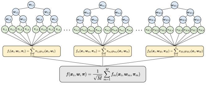
Figure 1: Schematics of an ensemble of M𝑀M soft trees. Tree internal nodes are indexed according to the breadth-first ordering.

Based on Kontschieder et al. (2015), we formulate a regression by soft trees. Figure 1 is a schematic image of an ensemble of M𝑀M soft trees. We define a data matrix 𝒙F×N𝒙superscript𝐹𝑁\bm{x}\in\mathbb{R}^{F\times N} for N𝑁N training samples {𝒙1,,𝒙N}subscript𝒙1subscript𝒙𝑁\{\bm{x}_{1},\dots,\bm{x}_{N}\} with F𝐹F features and define tree-wise parameter matrices for internal nodes 𝒘mF×𝒩subscript𝒘𝑚superscript𝐹𝒩\bm{w}_{m}\in\mathbb{R}^{F\times\mathcal{N}} and leaf nodes 𝝅m1×subscript𝝅𝑚superscript1\bm{\pi}_{m}\in\mathbb{R}^{1\times\mathcal{L}} for each tree m[M]={1,,M}𝑚delimited-[]𝑀1𝑀m\in[M]=\{1,\dots,M\} as

𝒙=(𝒙1𝒙N),𝒘m=(𝒘m,1𝒘m,𝒩),𝝅m=(πm,1,,πm,),formulae-sequence𝒙subscript𝒙1subscript𝒙𝑁formulae-sequencesubscript𝒘𝑚subscript𝒘𝑚1subscript𝒘𝑚𝒩subscript𝝅𝑚subscript𝜋𝑚1subscript𝜋𝑚\displaystyle\bm{x}=\left(\begin{array}[]{ccc}\mid&\ldots&\mid\\ \bm{x}_{1}&\ldots&\bm{x}_{N}\\ \mid&\ldots&\mid\end{array}\right),\quad\bm{w}_{m}=\left(\begin{array}[]{ccc}\mid&\ldots&\mid\\ \bm{w}_{m,1}&\ldots&\bm{w}_{m,\mathcal{N}}\\ \mid&\ldots&\mid\end{array}\right),\quad\bm{\pi}_{m}=\left(\pi_{m,1},\dots,\pi_{m,\mathcal{L}}\right),

where internal nodes (blue nodes in Figure 1) and leaf nodes (green nodes in Figure 1) are indexed from 111 to 𝒩𝒩\mathcal{N} and 111 to \mathcal{L}, respectively. 𝒩𝒩\mathcal{N} and \mathcal{L} may change across trees in general, while we assume that they are always fixed for simplicity throughout the paper. We also write horizontal concatenation of (column) vectors as 𝒙=(𝒙1,,𝒙N)F×N𝒙subscript𝒙1subscript𝒙𝑁superscript𝐹𝑁\bm{x}=(\bm{x}_{1},\dots,\bm{x}_{N})\in\mathbb{R}^{F\times N} and 𝒘m=(𝒘m,1,,𝒘m,𝒩)F×𝒩subscript𝒘𝑚subscript𝒘𝑚1subscript𝒘𝑚𝒩superscript𝐹𝒩\bm{w}_{m}=(\bm{w}_{m,1},\dots,\bm{w}_{m,\mathcal{N}})\in\mathbb{R}^{F\times\mathcal{N}}. Unlike hard decision trees, we consider a model in which every single leaf node []={1,,}delimited-[]1\ell\in[\mathcal{L}]=\{1,\dots,\mathcal{L}\} of a tree m𝑚m holds the probability that data will reach to it. Therefore, the splitting operation at an intermediate node n[𝒩]={1,,𝒩}𝑛delimited-[]𝒩1𝒩n\in[\mathcal{N}]=\{1,\dots,\mathcal{N}\} does not definitively decide splitting to the left or right. To provide an explicit form of the probabilistic tree splitting operation, we introduce the following binary relations that depend on the tree’s structure: n𝑛\ell\swarrow n (resp. n𝑛n\searrow\ell), which is true if a leaf \ell belongs to the left (resp. right) subtree of a node n𝑛n and false otherwise. We can now exploit μm,(𝒙i,𝒘m):F×F×𝒩[0,1]:subscript𝜇𝑚subscript𝒙𝑖subscript𝒘𝑚superscript𝐹superscript𝐹𝒩01\mu_{m,\ell}(\bm{x}_{i},\bm{w}_{m}):\mathbb{R}^{F}\times\mathbb{R}^{F\times\mathcal{N}}\to[0,1], a function that returns the probability that a sample 𝒙isubscript𝒙𝑖\bm{x}_{i} will reach a leaf \ell of the tree m𝑚m, as follows:

μm,(𝒙i,𝒘m)=n=1𝒩gm,n(𝒙i,𝒘m,n)𝟙n(1gm,n(𝒙i,𝒘m,n))𝟙n,subscript𝜇𝑚subscript𝒙𝑖subscript𝒘𝑚superscriptsubscriptproduct𝑛1𝒩subscript𝑔𝑚𝑛superscriptsubscript𝒙𝑖subscript𝒘𝑚𝑛subscript1𝑛superscript1subscript𝑔𝑚𝑛subscript𝒙𝑖subscript𝒘𝑚𝑛subscript1𝑛\displaystyle\mu_{m,\ell}(\bm{x}_{i},\bm{w}_{m})=\prod_{n=1}^{\mathcal{N}}g_{m,n}(\bm{x}_{i},\bm{w}_{m,n})^{\mathds{1}_{\ell\swarrow n}}\left(1-g_{m,n}(\bm{x}_{i},\bm{w}_{m,n})\right)^{\mathds{1}_{n\searrow\ell}}, (1)

where 𝟙Qsubscript1𝑄\mathds{1}_{Q} is an indicator function conditioned on the argument Q𝑄Q, i.e., 𝟙true=1subscript1true1\mathds{1}_{\text{true}}=1 and 𝟙false=0subscript1false0\mathds{1}_{\text{false}}=0, and gm,n:F×F[0,1]:subscript𝑔𝑚𝑛superscript𝐹superscript𝐹01g_{m,n}:\mathbb{R}^{F}\times\mathbb{R}^{F}\to[0,1] is a decision function at each internal node n𝑛n of a tree m𝑚m. To approximate decision tree splitting, the output of the decision function gm,nsubscript𝑔𝑚𝑛g_{m,n} should be between 0.00.00.0 and 1.01.01.0. If the output of a decision function takes only 0.00.00.0 or 1.01.01.0, the splitting operation is equivalent to hard splitting used in typical decision trees. We will define an explicit form of the decision function gm,nsubscript𝑔𝑚𝑛g_{m,n} in Equation (5) in the next section.

The prediction for each 𝒙isubscript𝒙𝑖\bm{x}_{i} from a tree m𝑚m with nodes parameterized by 𝒘msubscript𝒘𝑚\bm{w}_{m} and 𝝅msubscript𝝅𝑚\bm{\pi}_{m} is given by

fm(𝒙i,𝒘m,𝝅m)==1πm,μm,(𝒙i,𝒘m),subscript𝑓𝑚subscript𝒙𝑖subscript𝒘𝑚subscript𝝅𝑚superscriptsubscript1subscript𝜋𝑚subscript𝜇𝑚subscript𝒙𝑖subscript𝒘𝑚\displaystyle f_{m}(\bm{x}_{i},\bm{w}_{m},\bm{\pi}_{m})=\sum_{\ell=1}^{\mathcal{L}}\pi_{m,\ell}\mu_{m,\ell}(\bm{x}_{i},\bm{w}_{m}), (2)

where fm:F×F×𝒩×1×:subscript𝑓𝑚superscript𝐹superscript𝐹𝒩superscript1f_{m}:\mathbb{R}^{F}\times\mathbb{R}^{F\times\mathcal{N}}\times\mathbb{R}^{1\times\mathcal{L}}\to\mathbb{R}, and πm,subscript𝜋𝑚\pi_{m,\ell} denotes the response of a leaf \ell of the tree m𝑚m. This formulation means that the prediction output is the average of the leaf values πm,subscript𝜋𝑚\pi_{m,\ell} weighted by μm,(𝒙i,𝒘m)subscript𝜇𝑚subscript𝒙𝑖subscript𝒘𝑚\mu_{m,\ell}(\bm{x}_{i},\bm{w}_{m}), probability of assigning the sample 𝒙isubscript𝒙𝑖\bm{x}_{i} to the leaf \ell. If μm,(𝒙i,𝒘m)subscript𝜇𝑚subscript𝒙𝑖subscript𝒘𝑚\mu_{m,\ell}(\bm{x}_{i},\bm{w}_{m}) takes only 1.01.01.0 for one leaf and 0.00.00.0 for the other leaves, the behavior is equivalent to a typical decision tree prediction. In this model, 𝒘msubscript𝒘𝑚\bm{w}_{m} and 𝝅msubscript𝝅𝑚\bm{\pi}_{m} are updated during training with a gradient method.

While many empirical successes have been reported, theoretical analysis for soft tree ensemble models has not been sufficiently developed.

2.2 Neural tangent kernel

Given N𝑁N samples 𝒙F×N𝒙superscript𝐹𝑁\bm{x}\in\mathbb{R}^{F\times N}, the NTK induced by any model architecture at a training time τ𝜏\tau is formulated as a matrix 𝑯^τN×Nsuperscriptsubscript^𝑯𝜏superscript𝑁𝑁\widehat{\bm{H}}_{\tau}^{\ast}\in\mathbb{R}^{N\times N}, in which each (i,j)[N]×[N]𝑖𝑗delimited-[]𝑁delimited-[]𝑁(i,j)\in[N]\times[N] component is defined as

[𝑯^τ]ijΘ^τ(𝒙i,𝒙j)farbitrary(𝒙i,𝜽τ)𝜽τ,farbitrary(𝒙j,𝜽τ)𝜽τ,subscriptdelimited-[]superscriptsubscript^𝑯𝜏𝑖𝑗superscriptsubscript^Θ𝜏subscript𝒙𝑖subscript𝒙𝑗subscript𝑓arbitrarysubscript𝒙𝑖subscript𝜽𝜏subscript𝜽𝜏subscript𝑓arbitrarysubscript𝒙𝑗subscript𝜽𝜏subscript𝜽𝜏\displaystyle[\widehat{\bm{H}}_{\tau}^{\ast}]_{ij}\coloneqq\widehat{{\Theta}}_{\tau}^{\ast}(\bm{x}_{i},\bm{x}_{j})\coloneqq\left\langle\frac{\partial f_{\text{arbitrary}}\left(\bm{x}_{i},\bm{\theta}_{\tau}\right)}{\partial\bm{\theta}_{\tau}},\frac{\partial f_{\text{arbitrary}}\left(\bm{x}_{j},\bm{\theta}_{\tau}\right)}{\partial\bm{\theta}_{\tau}}\right\rangle, (3)

where ,\langle\cdot,\cdot\rangle denotes the inner product and 𝜽τPsubscript𝜽𝜏superscript𝑃\bm{\theta}_{\tau}\in\mathbb{R}^{P} is a concatenated vector of all the P𝑃P trainable model parameters at τ𝜏\tau. An asterisk “  ” indicates that the model is arbitrary. The model function farbitrary:F×P:subscript𝑓arbitrarysuperscript𝐹superscript𝑃f_{\text{arbitrary}}:\mathbb{R}^{F}\times\mathbb{R}^{P}\to\mathbb{R} used in Equation (3) is expected to be applicable to a variety of model structures. For the soft tree ensembles introduced in Section 2.1, the NTK is formulated as m=1Mn=1𝒩f(𝒙i,𝒘,𝝅)𝒘m,n,f(𝒙j,𝒘,𝝅)𝒘m,n+m=1M=1f(𝒙i,𝒘,𝝅)πm,,f(𝒙j,𝒘,𝝅)πm,superscriptsubscript𝑚1𝑀superscriptsubscript𝑛1𝒩𝑓subscript𝒙𝑖𝒘𝝅subscript𝒘𝑚𝑛𝑓subscript𝒙𝑗𝒘𝝅subscript𝒘𝑚𝑛superscriptsubscript𝑚1𝑀superscriptsubscript1𝑓subscript𝒙𝑖𝒘𝝅subscript𝜋𝑚𝑓subscript𝒙𝑗𝒘𝝅subscript𝜋𝑚\sum_{m=1}^{M}\sum_{n=1}^{\mathcal{N}}\left\langle\frac{\partial f\left(\bm{x}_{i},\bm{w},\bm{\pi}\right)}{\partial\bm{w}_{m,n}},\frac{\partial f\left(\bm{x}_{j},\bm{w},\bm{\pi}\right)}{\partial\bm{w}_{m,n}}\right\rangle+\sum_{m=1}^{M}\sum_{\ell=1}^{\mathcal{L}}\left\langle\frac{\partial f\left(\bm{x}_{i},\bm{w},\bm{\pi}\right)}{\partial\pi_{m,\ell}},\frac{\partial f\left(\bm{x}_{j},\bm{w},\bm{\pi}\right)}{\partial\pi_{m,\ell}}\right\rangle.

Within the limit of infinite width with a proper parameter scaling, a variety of properties have been discovered from the NTK induced by the MLP. For example, Jacot et al. (2018) showed the convergence of Θ^0MLP(𝒙i,𝒙j)superscriptsubscript^Θ0MLPsubscript𝒙𝑖subscript𝒙𝑗\widehat{{\Theta}}_{0}^{\mathrm{MLP}}(\bm{x}_{i},\bm{x}_{j}), which can vary with respect to parameters, to the unique limiting kernel ΘMLP(𝒙i,𝒙j)superscriptΘMLPsubscript𝒙𝑖subscript𝒙𝑗\Theta^{\mathrm{MLP}}(\bm{x}_{i},\bm{x}_{j}) at initialization in probability. Moreover, they also showed that the limiting kernel does not change during training in probability:

limwidthΘ^τMLP(𝒙i,𝒙j)=limwidthΘ^0MLP(𝒙i,𝒙j)=ΘMLP(𝒙i,𝒙j).subscriptwidthsuperscriptsubscript^Θ𝜏MLPsubscript𝒙𝑖subscript𝒙𝑗subscriptwidthsuperscriptsubscript^Θ0MLPsubscript𝒙𝑖subscript𝒙𝑗superscriptΘMLPsubscript𝒙𝑖subscript𝒙𝑗\displaystyle\lim_{\text{width}\to\infty}\widehat{\Theta}_{\tau}^{\mathrm{MLP}}(\bm{x}_{i},\bm{x}_{j})=\lim_{\text{width}\to\infty}\widehat{\Theta}_{0}^{\mathrm{MLP}}(\bm{x}_{i},\bm{x}_{j})=\Theta^{\mathrm{MLP}}(\bm{x}_{i},\bm{x}_{j}). (4)

This property helps in the analytical understanding of the model behavior. For example, with the squared loss and infinitesimal step size with learning rate η𝜂\eta, the training dynamics of gradient flow in function space coincides with kernel ridge-less regression with the limiting NTK. Such a property gives us a data-dependent generalization bound (Bartlett & Mendelson, 2003) related to the NTK and the prediction targets. In addition, if the NTK is positive definite, the training can achieve global convergence (Du et al., 2019a; Jacot et al., 2018).

Although a number of findings have been obtained using the NTK, they are mainly for typical neural networks such as MLP and ResNet (He et al., 2016), and the NTK theory has not yet been applied to tree models. The NTK theory is often used in the context of overparameterization, which is a subject of interest not only for the neural networks, but also for the tree models (Belkin et al., 2019; Karthikeyan et al., 2021; Tang et al., 2018).

3 Setup
Refer to caption
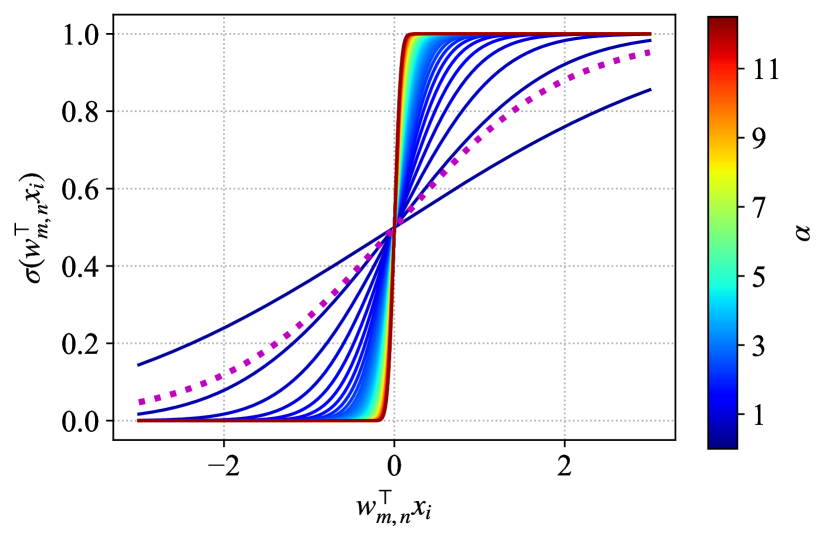
Figure 2: The scaled error function. We draw 50 lines with varying α𝛼\alpha by 0.250.250.25. A dotted magenta line shows a sigmoidsigmoid\operatorname{sigmoid} function, which is close to a scaled error function with α0.5similar-to𝛼0.5\alpha\sim 0.5.

We train model parameters 𝒘𝒘\bm{w} and 𝝅𝝅\bm{\pi} to minimize the squared loss using the gradient method, where 𝒘=(𝒘1,,𝒘M)𝒘subscript𝒘1subscript𝒘𝑀\bm{w}=(\bm{w}_{1},\dots,\bm{w}_{M}) and 𝝅=(𝝅1,,𝝅M)𝝅subscript𝝅1subscript𝝅𝑀\bm{\pi}=(\bm{\pi}_{1},\dots,\bm{\pi}_{M}). The tree structure is fixed during training. In order to use a known closed-form solution of the NTK (Williams, 1996; Lee et al., 2019), we use a scaled error function σ:(0,1):𝜎01\sigma:\mathbb{R}\to(0,1), resulting in the following decision function:

gm,n(𝒙i,𝒘m,n)subscript𝑔𝑚𝑛subscript𝒙𝑖subscript𝒘𝑚𝑛\displaystyle g_{m,n}(\bm{x}_{i},\bm{w}_{m,n}) =σ(𝒘m,n𝒙i)absent𝜎superscriptsubscript𝒘𝑚𝑛topsubscript𝒙𝑖\displaystyle=\sigma\left(\bm{w}_{m,n}^{\top}\bm{x}_{i}\right)
12erf(α𝒘m,n𝒙i)+12,absent12erf𝛼superscriptsubscript𝒘𝑚𝑛topsubscript𝒙𝑖12\displaystyle\coloneqq\frac{1}{2}\operatorname{erf}\left(\alpha\bm{w}_{m,n}^{\top}\bm{x}_{i}\right)+\frac{1}{2}, (5)

where erf(p)=2π0pet2dterf𝑝2𝜋superscriptsubscript0𝑝superscript𝑒superscript𝑡2differential-d𝑡\operatorname{erf}(p)=\frac{2}{\sqrt{\pi}}\int_{0}^{p}e^{-t^{2}}\mathrm{\leavevmode\nobreak\ d}t for p𝑝p\in\mathbb{R}. This scaled error function approximates a commonly used sigmoidsigmoid\operatorname{sigmoid} function. Since the bias term for the input of σ𝜎\sigma can be expressed inside of 𝒘𝒘\bm{w} by adding an element that takes a fixed constant value for all input of the soft trees 𝒙𝒙\bm{x}, we do not consider the bias for simplicity. The scaling factor α𝛼\alpha is introduced by Frosst & Hinton (2017) to avoid overly soft splitting. Figure 2 shows that the decision function becomes harder as α𝛼\alpha increases (from blue to red), and in the limit α𝛼\alpha\rightarrow\infty it coincides with the hard splitting used in typical decision trees.

When aggregating the output of multiple trees, we divide the sum of the tree outputs by the square root of the number of trees

f(𝒙i,𝒘,𝝅)=1Mm=1Mfm(𝒙i,𝒘m,𝝅m).𝑓subscript𝒙𝑖𝒘𝝅1𝑀superscriptsubscript𝑚1𝑀subscript𝑓𝑚subscript𝒙𝑖subscript𝒘𝑚subscript𝝅𝑚\displaystyle f(\bm{x}_{i},\bm{w},\bm{\pi})=\frac{1}{\sqrt{M}}\sum_{m=1}^{M}f_{m}(\bm{x}_{i},\bm{w}_{m},\bm{\pi}_{m}). (6)

This 1/M1𝑀1/\sqrt{M} scaling is known to be essential in the existing NTK literature to use the weak law of the large numbers (Jacot et al., 2018). On top of Equation (6), we initialize each of model parameters 𝒘m,nsubscript𝒘𝑚𝑛\bm{w}_{m,n} and πm,subscript𝜋𝑚\pi_{m,\ell} with zero-mean i.i.d. Gaussians with unit variances. We refer such a parameterization as NTK initialization. In this paper, we consider a model such that all M𝑀M trees have the same perfect binary tree structure, a common setting for soft tree ensembles (Popov et al., 2020; Kontschieder et al., 2015; Hazimeh et al., 2020).

4 Theoretical results

4.1 Basic properties of the TNTK

The NTK in Equation (3) induced by the soft tree ensembles is referred to here as the TNTK and denoted by Θ^0(d)(𝒙i,𝒙j)subscriptsuperscript^Θ𝑑0subscript𝒙𝑖subscript𝒙𝑗\widehat{\Theta}^{(d)}_{0}(\bm{x}_{i},\bm{x}_{j}) the TNTK at initialization induced by the ensemble of trees with depth d𝑑d. In this section, we show the properties of the TNTK that are important for understanding the training behavior of the soft tree ensembles.

4.1.1 TNTK for infinite tree ensembles

First, we show the formula of the TNTK at initialization, which converges when considering the limit of infinite trees (M)𝑀(M\rightarrow\infty).

Theorem 1.

Let 𝐮F𝐮superscript𝐹\bm{u}\in\mathbb{R}^{F} be any column vector sampled from zero-mean i.i.d. Gaussians with unit variance. The TNTK for an ensemble of soft perfect binary trees with tree depth d𝑑d converges in probability to the following deterministic kernel as M𝑀M\to\infty,

Θ(d)(𝒙i,𝒙j)superscriptΘ𝑑subscript𝒙𝑖subscript𝒙𝑗\displaystyle{\Theta}^{(d)}(\bm{x}_{i},\bm{x}_{j}) limMΘ^0(d)(𝒙i,𝒙j)absentsubscript𝑀subscriptsuperscript^Θ𝑑0subscript𝒙𝑖subscript𝒙𝑗\displaystyle\coloneqq\lim_{M\rightarrow\infty}\widehat{\Theta}^{(d)}_{0}(\bm{x}_{i},\bm{x}_{j})
=2ddΣ(𝒙i,𝒙j)(𝒯(𝒙i,𝒙j))d1𝒯˙(𝒙i,𝒙j)contribution from inner nodes+(2𝒯(𝒙i,𝒙j))dcontribution from leaves,absentsubscriptsuperscript2𝑑𝑑Σsubscript𝒙𝑖subscript𝒙𝑗superscript𝒯subscript𝒙𝑖subscript𝒙𝑗𝑑1˙𝒯subscript𝒙𝑖subscript𝒙𝑗contribution from inner nodessubscriptsuperscript2𝒯subscript𝒙𝑖subscript𝒙𝑗𝑑contribution from leaves\displaystyle=\underbrace{2^{d}d\leavevmode\nobreak\ \Sigma(\bm{x}_{i},\bm{x}_{j})(\mathcal{T}(\bm{x}_{i},\bm{x}_{j}))^{d-1}\dot{\mathcal{T}}(\bm{x}_{i},\bm{x}_{j})}_{\text{contribution from inner nodes}}+\underbrace{(2\mathcal{T}(\bm{x}_{i},\bm{x}_{j}))^{d}}_{\text{contribution from leaves}}, (7)

where Σ(𝐱i,𝐱j)𝐱i𝐱jΣsubscript𝐱𝑖subscript𝐱𝑗superscriptsubscript𝐱𝑖topsubscript𝐱𝑗\Sigma(\bm{x}_{i},\bm{x}_{j})\coloneqq\bm{x}_{i}^{\top}\bm{x}_{j}, 𝒯(𝐱i,𝐱j)𝔼[σ(𝐮𝐱i)σ(𝐮𝐱j)]𝒯subscript𝐱𝑖subscript𝐱𝑗𝔼delimited-[]𝜎superscript𝐮topsubscript𝐱𝑖𝜎superscript𝐮topsubscript𝐱𝑗\mathcal{T}(\bm{x}_{i},\bm{x}_{j})\coloneqq\mathbb{E}[\sigma(\bm{u}^{\top}\bm{x}_{i})\sigma(\bm{u}^{\top}\bm{x}_{j})], and 𝒯˙(𝐱i,𝐱j)𝔼[σ˙(𝐮𝐱i)σ˙(𝐮𝐱j)]˙𝒯subscript𝐱𝑖subscript𝐱𝑗𝔼delimited-[]˙𝜎superscript𝐮topsubscript𝐱𝑖˙𝜎superscript𝐮topsubscript𝐱𝑗\dot{\mathcal{T}}(\bm{x}_{i},\bm{x}_{j})\coloneqq\mathbb{E}[\dot{\sigma}(\bm{u}^{\top}\bm{x}_{i})\dot{\sigma}(\bm{u}^{\top}\bm{x}_{j})]. Moreover, 𝒯(𝐱i,𝐱j)𝒯subscript𝐱𝑖subscript𝐱𝑗\mathcal{T}(\bm{x}_{i},\bm{x}_{j}) and 𝒯˙(𝐱i,𝐱j)˙𝒯subscript𝐱𝑖subscript𝐱𝑗\dot{\mathcal{T}}(\bm{x}_{i},\bm{x}_{j}) are analytically obtained in the closed-form as

𝒯(𝒙i,𝒙j)𝒯subscript𝒙𝑖subscript𝒙𝑗\displaystyle\mathcal{T}(\bm{x}_{i},\bm{x}_{j}) =12πarcsin(α2Σ(𝒙i,𝒙j)(α2Σ(𝒙i,𝒙i)+0.5)(α2Σ(𝒙j,𝒙j)+0.5))+14,absent12𝜋superscript𝛼2Σsubscript𝒙𝑖subscript𝒙𝑗superscript𝛼2Σsubscript𝒙𝑖subscript𝒙𝑖0.5superscript𝛼2Σsubscript𝒙𝑗subscript𝒙𝑗0.514\displaystyle=\!\frac{1}{2\pi}\arcsin\!\left(\!\frac{\alpha^{2}\Sigma(\bm{x}_{i},\bm{x}_{j})}{\sqrt{(\alpha^{2}\Sigma(\bm{x}_{i},\bm{x}_{i})+0.5)(\alpha^{2}\Sigma(\bm{x}_{j},\bm{x}_{j})+0.5)}}\right)\!+\!\frac{1}{4}, (8)
𝒯˙(𝒙i,𝒙j)˙𝒯subscript𝒙𝑖subscript𝒙𝑗\displaystyle\dot{\mathcal{T}}(\bm{x}_{i},\bm{x}_{j}) =α2π1(1+2α2Σ(𝒙i,𝒙i))(1+2α2Σ(𝒙j,𝒙j))4α4Σ(𝒙i,𝒙j)2.absentsuperscript𝛼2𝜋112superscript𝛼2Σsubscript𝒙𝑖subscript𝒙𝑖12superscript𝛼2Σsubscript𝒙𝑗subscript𝒙𝑗4superscript𝛼4Σsuperscriptsubscript𝒙𝑖subscript𝒙𝑗2\displaystyle=\!\frac{\alpha^{2}}{\pi}\frac{1}{\sqrt{\left(1+2\alpha^{2}\Sigma(\bm{x}_{i},\bm{x}_{i})\right)(1+2\alpha^{2}\Sigma(\bm{x}_{j},\bm{x}_{j}))\!-\!4\alpha^{4}\Sigma(\bm{x}_{i},\bm{x}_{j})^{2}}}. (9)

The dot used in σ˙(𝒖𝒙i)˙𝜎superscript𝒖topsubscript𝒙𝑖\dot{\sigma}(\bm{u}^{\top}\bm{x}_{i}) means the first derivative: αe(α𝒖𝒙i)2/π𝛼superscript𝑒superscript𝛼superscript𝒖topsubscript𝒙𝑖2𝜋\alpha e^{-(\alpha\bm{u}^{\top}\bm{x}_{i})^{2}}/\sqrt{\pi}, and 𝔼[]𝔼delimited-[]\mathbb{E}[\cdot] means the expectation. The scalar π𝜋\pi in Equation (8) and Equation (9) is the circular constant, and 𝒖𝒖\bm{u} corresponds to 𝒘m,nsubscript𝒘𝑚𝑛\bm{w}_{m,n} at an arbitrary internal node. The proof is given by induction. We can derive the formula of the limiting TNTK by treating the number of trees in a tree ensemble like the width of the hidden layer in MLP, although the MLP and the soft tree ensemble are apparently different models. Due to space limitations, detailed proofs are given in the supplementary material.

Refer to caption
Figure 3: Left: An empirical demonstration of convergence of Θ^0(𝒙i,𝒙j)subscript^Θ0subscript𝒙𝑖subscript𝒙𝑗\widehat{\Theta}_{0}(\bm{x}_{i},\bm{x}_{j}) to the fixed limit Θ(𝒙i,𝒙j)Θsubscript𝒙𝑖subscript𝒙𝑗{{\Theta}}(\bm{x}_{i},\bm{x}_{j}) as M𝑀M increases. Two simple inputs are considered: 𝒙i={1,0}subscript𝒙𝑖10\bm{x}_{i}=\{1,0\} and 𝒙j={cos(β),sin(β)}subscript𝒙𝑗𝛽𝛽\bm{x}_{j}=\{\cos(\beta),\sin(\beta)\} with β=[0,π]𝛽0𝜋\beta=[0,\pi]. The TNTK Θ^0(3)(𝒙i,𝒙j)subscriptsuperscript^Θ30subscript𝒙𝑖subscript𝒙𝑗\widehat{\Theta}^{(3)}_{0}(\bm{x}_{i},\bm{x}_{j}) with α=2.0𝛼2.0\alpha=2.0 is calculated 101010 times with parameter re-initialization for each of the M=16𝑀16M=16, 646464, 256256256, 102410241024, and 409640964096. Center and Right: Parameter dependency of the convergence. The vertical axis corresponds to the averaged error between the 𝑯^0subscript^𝑯0\widehat{\bm{H}}_{0} and the 𝑯limM𝑯^0𝑯subscript𝑀subscript^𝑯0\bm{H}\coloneqq\lim_{M\to\infty}\widehat{\bm{H}}_{0} for 505050 random unit vectors of length F=5𝐹5F=5. The dashed lines are plotted only for showing the slope. The error bars show the standard deviations of 101010 executions.

We demonstrate convergence of the TNTK in Figure 3. We empirically observe that the TNTK induced by sufficiently many soft trees converges to the limiting TNTK given in Equation (7). The kernel values induced by an finite ensemble are already close to the limiting TNTK if the number of trees is larger than several hundreds, which is a typical order of the number of trees in practical applications111For example, Popov et al. (2020) uses 204820482048 trees.. Therefore, it is reasonable to analyze soft tree ensembles via the TNTK.

By comparing Equation (7) and the limiting NTK induced by a two-layer perceptron (shown in the supplementary material), we can immediately derive the following when the tree depth is 111.

Corollary 1.

If the splitting function at the tree internal node is the same as the activation function of the neural network, the limiting TNTK obtained from a soft tree ensemble of depth 111 is equivalent to the limiting NTK generated by a two-layer perceptron up to constant multiple.

For any tree depth larger than 111, the limiting NTK induced by the MLP with any number of layers (Arora et al., 2019, shown in the supplementary material) and the limiting TNTK do not match. This implies that the hierarchical splitting structure is a distinctive feature of soft tree ensembles.

4.1.2 Positive definiteness of the limiting TNTK

Since the loss surface of a large model is expected to be highly non-convex, understanding the good empirical trainability of overparameterized models remains an open problem (Dauphin et al., 2014). The positive definiteness of the limiting kernel is one of the most important conditions for achieving global convergence (Du et al., 2019a; Jacot et al., 2018). Jacot et al. (2018) showed that the conditions 𝒙i2=1subscriptnormsubscript𝒙𝑖21\|\bm{x}_{i}\|_{2}=1 for all i[N]𝑖delimited-[]𝑁i\in[N] and 𝒙i𝒙j(ij)subscript𝒙𝑖subscript𝒙𝑗𝑖𝑗\bm{x}_{i}\neq\bm{x}_{j}\leavevmode\nobreak\ (i\neq j) are necessary for the positive definiteness of the NTK induced by the MLP for an input set. As for the TNTK, since the formulation (Equation (7)) is different from that of typical neural networks such as an MLP, it is not clear whether or not the limiting TNTK is positive definite.

We prove that the TNTK induced by infinite trees is also positive definite under the same condition for the MLP.

Proposition 1.

For infinitely many soft trees with any depth and the NTK initialization, the limiting TNTK is positive definite if 𝐱i2=1subscriptnormsubscript𝐱𝑖21\|\bm{x}_{i}\|_{2}=1 for all i[N]𝑖delimited-[]𝑁i\in[N] and 𝐱i𝐱j(ij)subscript𝐱𝑖subscript𝐱𝑗𝑖𝑗\bm{x}_{i}\neq\bm{x}_{j}\leavevmode\nobreak\ (i\neq j).

The proof is provided in the supplementary material. Similar to the discussion for the MLP (Du et al., 2019a; Jacot et al., 2018), if the limiting TNTK is constant during training, the positive definiteness of the limiting TNTK at initialization indicates that training of the infinite trees with a gradient method can converge to the global minimum. The constantness of the limiting TNTK during training is shown in the following section.

4.1.3 Change of the TNTK during training

We prove that the TNTK hardly changes from its initial value during training when considering an ensemble of infinite trees with finite α𝛼\alpha (used in Equation (5)).

Theorem 2.

Let λminsubscript𝜆min\lambda_{\text{min}} and λmaxsubscript𝜆max\lambda_{\text{max}} be the minimum and maximum eigenvalues of the limiting TNTK. Assume that the limiting TNTK is positive definite for input sets. For soft tree ensemble models with the NTK initialization and a positive finite scaling factor α𝛼\alpha trained under gradient flow with a learning rate η<2/(λmin+λmax)𝜂2subscript𝜆minsubscript𝜆max\eta<2/(\lambda_{\text{min}}+\lambda_{\text{max}}), we have, with high probability,

sup|Θ^τ(d)(𝒙i,𝒙j)Θ^0(d)(𝒙i,𝒙j)|=𝒪(1M).supremumsuperscriptsubscript^Θ𝜏𝑑subscript𝒙𝑖subscript𝒙𝑗superscriptsubscript^Θ0𝑑subscript𝒙𝑖subscript𝒙𝑗𝒪1𝑀\displaystyle\sup\left|{\widehat{{\Theta}}}_{\tau}^{(d)}\left(\bm{x}_{i},\bm{x}_{j}\right)-\widehat{{{\Theta}}}_{0}^{(d)}\left(\bm{x}_{i},\bm{x}_{j}\right)\right|=\mathcal{O}\left(\frac{1}{\sqrt{M}}\right). (10)

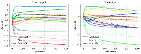
The complete proof is provided in the supplementary material. Figure 4 shows that the training trajectory analytically obtained (Jacot et al., 2018; Lee et al., 2019) from the limiting TNTK and the trajectory during gradient descent training become similar as the number of trees increases, demonstrating the validity of using the TNTK framework to analyze the training behavior.
Refer to caption
Figure 4: Output dynamics for train and test data points. The color of each line corresponds to each data point. Soft tree ensembles with d=3𝑑3d=3, α=2.0𝛼2.0\alpha=2.0 are trained by a full-batch gradient descent with a learning rate of 0.10.10.1. Initial outputs are shifted to zero (Chizat et al., 2019). There are 101010 randomly generated training points and 101010 randomly generated test data points, and their dimension F=5𝐹5F=5. The prediction targets are also randomly generated. Let 𝑯(𝒙,𝒙)N×N𝑯𝒙superscript𝒙superscript𝑁superscript𝑁\bm{H}(\bm{x},\bm{x}^{\prime})\in\mathbb{R}^{N\times{N^{\prime}}} be the limiting NTK matrix for two input matrices and 𝑰𝑰\bm{I} be an identity matrix. For analytical results, we draw the trajectory f(𝒗,𝜽τ)=𝑯(𝒗,𝒙)𝑯(𝒙,𝒙)1(𝑰exp[η𝑯(𝒙,𝒙)τ])𝒚𝑓𝒗subscript𝜽𝜏𝑯𝒗𝒙𝑯superscript𝒙𝒙1𝑰𝜂𝑯𝒙𝒙𝜏𝒚f(\bm{v},\bm{\theta}_{\tau})=\bm{H}(\bm{v},\bm{x})\bm{H}(\bm{x},\bm{x})^{-1}(\bm{I}-\exp[-\eta\bm{H}(\bm{x},\bm{x})\tau])\bm{y} (Lee et al., 2019) using the limiting TNTK (Equation (7)), where 𝒗F𝒗superscript𝐹\bm{v}\in\mathbb{R}^{F} is an arbitrary input and 𝒙F×N𝒙superscript𝐹𝑁\bm{x}\in\mathbb{R}^{F\times{N}} and 𝒚N𝒚superscript𝑁\bm{y}\in\mathbb{R}^{N} are the training dataset and the targets, respectively.

Remarks.  In the limit of infinitely large α𝛼\alpha, which corresponds to a hard decision tree splitting (Figure 2), it should be noted that this theorem does not hold because of the lack of local Lipschitzness (Lee et al., 2019), which is the fundamental property for this proof. Therefore the change in the TNTK during training is no longer necessarily asymptotic to zero, even if the number of trees is infinite. This means that understanding the hard decision tree’s behavior using the TNTK is not straightforward.

4.2 Implications for practical techniques

In this section, from the viewpoint of the TNTK, we discuss the training techniques that have been used in practice.

4.2.1 Influence of the oblivious tree structure

Refer to caption
Figure 5: Left: Normal Tree, Right: Oblivious Tree. The rules for splitting in the same depth are shared across the same depth in the oblivious tree, while πm,subscript𝜋𝑚{\pi}_{m,\ell} on leaves can be different.

An oblivious tree is a practical tree model architecture where the rules across decision tree splitting are shared across the same depth as illustrated in Figure 5. Since the number of the splitting decision calculation can be reduced from 𝒪(2d)𝒪superscript2𝑑\mathcal{O}(2^{d}) to 𝒪(d)𝒪𝑑\mathcal{O}(d), the oblivious tree structure is used in various open-source libraries such as CatBoost (Prokhorenkova et al., 2018) and NODE (Popov et al., 2020). However, the reason for the good empirical performance of oblivious trees is non-trivial despite weakening the expressive power due to parameter sharing.

We find that the oblivious tree structure does not change the limiting TNTK from the non-oblivious one. This happens because, even with parameter sharing at splitting nodes, leaf parameters 𝝅𝝅\bm{\pi} are not shared, resulting in independence between outputs of left and right subtrees.

Theorem 3.

The TNTK with the perfect binary tree ensemble and the TNTK of its corresponding oblivious tree ensemble obtained via parameter sharing converge to the same kernel in probability in the limit of infinite trees (M)𝑀(M\rightarrow\infty).

The complete proof is in the supplementary material. Note that leaf values 𝝅𝝅\bm{\pi} do not have to be the same for oblivious and non-oblivious trees. This theorem supports the recent success of tree ensemble models with the oblivious tree structures.

4.2.2 Effect of the decision function modification

Refer to caption
Figure 6: Parameter dependencies of 𝒯(𝒙i,𝒙j)𝒯subscript𝒙𝑖subscript𝒙𝑗\mathcal{T}(\bm{x}_{i},\bm{x}_{j}), 𝒯˙(𝒙i,𝒙j)˙𝒯subscript𝒙𝑖subscript𝒙𝑗\dot{\mathcal{T}}(\bm{x}_{i},\bm{x}_{j}), and Θ(d)(𝒙i,𝒙j)superscriptΘ𝑑subscript𝒙𝑖subscript𝒙𝑗{\Theta}^{(d)}(\bm{x}_{i},\bm{x}_{j}). The vertical axes are normalized so that the value is 111 when the inner product of the inputs is 111. The input vector size is normalized to be one. For the three figures on the left, the line color is determined by α𝛼\alpha, and for the figure on the right, it is determined by the depth of the tree.

Practically, based on the commonly used sigmoidsigmoid\operatorname{sigmoid} function, a variety of functions have been proposed for the splitting operation. By considering a large scaling factor α𝛼\alpha in Equation (5), we can envisage situations in which there are practically used hard functions, such as two-class sparsemaxsparsemax\operatorname{sparsemax}, σ(x)=sparsemax([x,0])𝜎𝑥sparsemax𝑥0\sigma(x)=\mathrm{sparsemax}([x,0]) (Martins & Astudillo, 2016), and two-class entmaxentmax\operatorname{entmax}, σ(x)=entmax([x,0])𝜎𝑥entmax𝑥0\sigma(x)=\mathrm{entmax}([x,0]) (Peters et al., 2019). Figure 6 shows α𝛼\alpha dependencies of TNTK parameters. Equation (7) means that the TNTK is formulated by multiplying 𝒯(𝒙i,𝒙j)𝒯subscript𝒙𝑖subscript𝒙𝑗\mathcal{T}(\bm{x}_{i},\bm{x}_{j}) and 𝒯˙(𝒙i,𝒙j)˙𝒯subscript𝒙𝑖subscript𝒙𝑗\mathcal{\dot{T}}(\bm{x}_{i},\bm{x}_{j}) to the linear kernel Σ(𝒙i,𝒙j)Σsubscript𝒙𝑖subscript𝒙𝑗\Sigma(\bm{x}_{i},\bm{x}_{j}). On the one hand, 𝒯(𝒙i,𝒙j)𝒯subscript𝒙𝑖subscript𝒙𝑗\mathcal{T}(\bm{x}_{i},\bm{x}_{j}) and 𝒯˙(𝒙i,𝒙j)˙𝒯subscript𝒙𝑖subscript𝒙𝑗\mathcal{\dot{T}}(\bm{x}_{i},\bm{x}_{j}) with small α𝛼\alpha are almost constant, even for different input inner products, resulting in the almost linear TNTK. On the other hand, the nonlinearity increases as α𝛼\alpha increases. For Figure 2, the original sigmoidsigmoid\operatorname{sigmoid} function corresponds to a scaled error function for α0.5similar-to𝛼0.5\alpha\sim 0.5, which induces almost the linear kernel. Although a closed-form TNTK using sigmoidsigmoid\operatorname{sigmoid} as a decision function has not been obtained, its kernel is expected to be almost linear. Therefore, from the viewpoint of the TNTK, an adjustment of the decision function (Frosst & Hinton, 2017; Popov et al., 2020; Hazimeh et al., 2020) can be interpreted as an escape from the linear kernel behavior.

4.2.3 Degeneracy caused by deep trees

As the depth increases, 𝒯(𝒙i,𝒙j)𝒯subscript𝒙𝑖subscript𝒙𝑗\mathcal{T}(\bm{x}_{i},\bm{x}_{j}) defined in Equation (8), which consists of the arcsine function, is multiplied multiple times to calculate the limiting TNTK in Equation (7). Therefore, when we increase the depth too much, the resulting TNTK exhibits degeneracy: its output values are almost the same as each other’s, even though the input’s inner products are different. The rightmost panel of Figure 6 shows such degeneracy behavior. In terms of kernel regression, models using a kernel that gives almost the same inner product to all data except those that are quite close to each other are expected to have poor generalization performance. Such behavior is observed in our numerical experiments (Section 5). In practical applications, overly deep soft or hard decision trees are not usually used because overly deep trees show poor performance (Luo et al., 2021), which is supported by the degeneracy of the TNTK.

5 Numerical experiments

Setup.  We present our experimental results on 909090 classification tasks in the UCI database (Dua & Graff, 2017), with fewer than 500050005000 data points, as in Arora et al. (2020). We performed kernel regression using the limiting TNTK defined in Equation (7) with varying the tree depth (d𝑑d) and the scaling (α𝛼\alpha) of the decision function. The limiting TNTK does not change during training for an infinite ensemble of soft trees (Theorem 2); therefore, predictions from that model are equivalent to kernel regression using the limiting TNTK (Jacot et al., 2018). To consider the ridge-less situation, regularization strength is set to be 1.0×1081.0superscript1081.0\times 10^{-8}, a very small constant. By way of comparison, performances of the kernel regression with the MLP-induced NTK (Jacot et al., 2018) and the RBF kernel are also reported. For the MLP-induced NTK, we use ReLUReLU\operatorname{ReLU} for the activation function. We follow the procedures of Arora et al. (2020) and Fernández-Delgado et al. (2014): We report 444-fold cross-validation performance with random data splitting. To tune parameters, all available training samples are randomly split into one training and one validation set, while imposing that each class has the same number of training and validation samples. Then the parameter with the best validation accuracy is selected. Other details are provided in the supplementary material.
Refer to caption
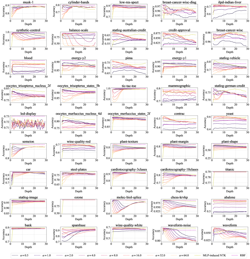
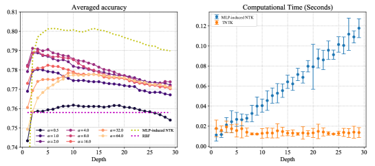
Figure 7: Left: Averaged accuracy over 909090 datasets. The performances of the kernel regression with the MLP-induced NTK and the RBF kernel are shown for comparison. Since the depth is not a hyperparameter of the RBF kernel, performance is shown by a horizontal line. The statistical significance is also assessed in the supplementary material. Right: Running time for kernel computation. The input dataset has 300300300 samples with 101010 features. Feature values are generated by zero-mean i.i.d Gaussian with unit variance. The error bars show the standard deviations of 101010 executions.
Table 1: Performance win rate against the MLP-induced NTK. We tune the depth from d=1𝑑1d=1 to 292929 for the dataset-wise comparison for both the TNTK and the MLP-induced NTK. For the RBF kernel, 303030 different hyperparameters are tried. Detailed results are in the supplementary material.
TNTK RBF
α𝛼\alpha 0.50.50.5 1.01.01.0 2.02.02.0 4.04.04.0 8.08.08.0 16.016.016.0 32.032.032.0 64.064.064.0
Win rate (%) 13.613.613.6 18.818.818.8 22.222.222.2 28.628.628.6 32.532.532.5 31.631.631.6 34.934.934.9 27.227.227.2 11.811.811.8

Comparison to the MLP.  The left panel of Figure 7 shows the averaged performance as a function of the depth. Although the TNTK with properly tuned parameters tend to be better than those obtained with the RBF kernel, they are often inferior to the MLP-induced NTK. The results support the good performance of the MLP-induced NTK (Arora et al., 2020). However, it should be noted that when we look at each dataset one by one, the TNTK is superior to the MLP-induced NTK by more than 303030 percent of the dataset, as shown in Table 1. This is a case where the characteristics of data and the inductive bias of the model fit well together. In addition, although the computational cost of the MLP-induced NTK is linear with respect to the depth of the model because of the recursive computation (Jacot et al., 2018), the computational cost of the TNTK does not depend on the depth, as shown in Equation (7). This results in much faster computation than the MLP-induced NTK when the depth increases, as illustrated in the right panel of Figure 7. Even if the MLP-induced NTK is better in prediction accuracy, the TNTK may be used in practical cases as a trade-off for computational complexity. Arora et al. (2019) proposed the use of the NTK for a neural architecture search (Elsken et al., 2019; Chen et al., 2021). In such applications, the fast computation of the kernel in various architectures can be a benefit. We leave extensions of this idea to tree models as future work.

Consistency with implications from the TNTK theory.  When we increase the tree depth, we initially observe an improvement in performance, after which the performance gradually decreases. This behavior is consistent with the performance deterioration due to degeneracy (Section 4.2.3), similar to that reported for neural networks without skip-connection (Huang et al., 2020), shown by a dotted yellow line. The performance improvement by adjusting α𝛼\alpha in the decision function (Frosst & Hinton, 2017) is also observed. Performances with hard (α>0.5𝛼0.5\alpha>0.5) decision functions are always better than the sigmoidsigmoid\operatorname{sigmoid}-like function (α=0.5𝛼0.5\alpha=0.5, as shown in Figure 2).

6 Conclusion

In this paper, we have introduced and studied the Tree Neural Tangent Kernel (TNTK) by considering the ensemble of infinitely many soft trees. The TNTK provides new insights into the behavior of the infinite ensemble of soft trees, such as the effect of the oblivious tree structure and the degeneracy of the TNTK induced by the deepening of the trees. In numerical experiments, we have observed the degeneracy phenomena induced by the deepening of the soft tree model, which is suggested by our theoretical results. To date, the NTK theory has been mostly applied to neural networks, and our study is the first to apply it to the tree model. Therefore our study represents a milestone in the development of the NTK theory.

Acknowledgement

This work was supported by JSPS KAKENHI (Grant Number JP21H03503d, Japan), JST PRESTO (Grant Number JPMJPR1855, Japan), and JST FOREST (Grant Number JPMJFR206J, Japan).

References

  • Alemohammad et al. (2021) Sina Alemohammad, Zichao Wang, Randall Balestriero, and Richard Baraniuk. The Recurrent Neural Tangent Kernel. In International Conference on Learning Representations, 2021.
  • Arik & Pfister (2019) Sercan Ömer Arik and Tomas Pfister. TabNet: Attentive Interpretable Tabular Learning. CoRR, abs/1908.07442, 2019.
  • Arora et al. (2019) Sanjeev Arora, Simon S Du, Wei Hu, Zhiyuan Li, Russ R Salakhutdinov, and Ruosong Wang. On Exact Computation with an Infinitely Wide Neural Net. In Advances in Neural Information Processing Systems, volume 32, 2019.
  • Arora et al. (2020) Sanjeev Arora, Simon S. Du, Zhiyuan Li, Ruslan Salakhutdinov, Ruosong Wang, and Dingli Yu. Harnessing the Power of Infinitely Wide Deep Nets on Small-data Tasks. In International Conference on Learning Representations, 2020.
  • Bartlett & Mendelson (2003) Peter L. Bartlett and Shahar Mendelson. Rademacher and Gaussian Complexities: Risk Bounds and Structural Results. Journal of Machine Learning Research, 3, 2003.
  • Belkin et al. (2019) Mikhail Belkin, Daniel Hsu, Siyuan Ma, and Soumik Mandal. Reconciling modern machine-learning practice and the classical bias–variance trade-off. Proceedings of the National Academy of Sciences, 116(32), 2019.
  • Breiman et al. (1984) Leo Breiman, Jerome Friedman, Charles J. Stone, and R.A. Olshen. Classification and Regression Trees. Chapman and Hall/CRC, 1984.
  • Chen et al. (2021) Wuyang Chen, Xinyu Gong, and Zhangyang Wang. Neural Architecture Search on ImageNet in Four GPU Hours: A Theoretically Inspired Perspective. In International Conference on Learning Representations, 2021.
  • Chizat et al. (2019) Lénaïc Chizat, Edouard Oyallon, and Francis Bach. On Lazy Training in Differentiable Programming. In Advances in Neural Information Processing Systems, volume 32, 2019.
  • Dauphin et al. (2014) Yann N Dauphin, Razvan Pascanu, Caglar Gulcehre, Kyunghyun Cho, Surya Ganguli, and Yoshua Bengio. Identifying and attacking the saddle point problem in high-dimensional non-convex optimization. In Advances in Neural Information Processing Systems, volume 27, 2014.
  • Du et al. (2019a) Simon Du, Jason Lee, Haochuan Li, Liwei Wang, and Xiyu Zhai. Gradient Descent Finds Global Minima of Deep Neural Networks. In Proceedings of the 36th International Conference on Machine Learning, 2019a.
  • Du et al. (2019b) Simon S Du, Kangcheng Hou, Russ R Salakhutdinov, Barnabas Poczos, Ruosong Wang, and Keyulu Xu. Graph Neural Tangent Kernel: Fusing Graph Neural Networks with Graph Kernels. In Advances in Neural Information Processing Systems, volume 32, 2019b.
  • Dua & Graff (2017) Dheeru Dua and Casey Graff. UCI Machine Learning Repository, 2017. URL http://archive.ics.uci.edu/ml.
  • Elsken et al. (2019) Thomas Elsken, Jan Hendrik Metzen, and Frank Hutter. Neural Architecture Search: A Survey. Journal of Machine Learning Research, 20(55):1–21, 2019.
  • Fernández-Delgado et al. (2014) Manuel Fernández-Delgado, Eva Cernadas, Senén Barro, and Dinani Amorim. Do we Need Hundreds of Classifiers to Solve Real World Classification Problems? Journal of Machine Learning Research, 15, 2014.
  • Frosst & Hinton (2017) Nicholas Frosst and Geoffrey E. Hinton. Distilling a Neural Network Into a Soft Decision Tree. CoRR, 2017.
  • Hazimeh et al. (2020) Hussein Hazimeh, Natalia Ponomareva, Petros Mol, Zhenyu Tan, and Rahul Mazumder. The Tree Ensemble Layer: Differentiability meets Conditional Computation. In Proceedings of the 37th International Conference on Machine Learning, volume 119, 2020.
  • He et al. (2016) Kaiming He, Xiangyu Zhang, Shaoqing Ren, and Jian Sun. Deep Residual Learning for Image Recognition. In 2016 IEEE Conference on Computer Vision and Pattern Recognition (CVPR), 2016.
  • Huang et al. (2020) Kaixuan Huang, Yuqing Wang, Molei Tao, and Tuo Zhao. Why Do Deep Residual Networks Generalize Better than Deep Feedforward Networks? — A Neural Tangent Kernel Perspective. In Advances in Neural Information Processing Systems, volume 33, 2020.
  • Jacot et al. (2018) Arthur Jacot, Franck Gabriel, and Clement Hongler. Neural Tangent Kernel: Convergence and Generalization in Neural Networks. In Advances in Neural Information Processing Systems 31. 2018.
  • Jordan & Jacobs (1993) M.I. Jordan and R.A. Jacobs. Hierarchical mixtures of experts and the EM algorithm. In Proceedings of 1993 International Conference on Neural Networks, volume 2, 1993.
  • Karthikeyan et al. (2021) Ajaykrishna Karthikeyan, Naman Jain, Nagarajan Natarajan, and Prateek Jain. Learning Accurate Decision Trees with Bandit Feedback via Quantized Gradient Descent. CoRR, 2021.
  • Ke et al. (2019) Guolin Ke, Zhenhui Xu, Jia Zhang, Jiang Bian, and Tie-Yan Liu. DeepGBM: A Deep Learning Framework Distilled by GBDT for Online Prediction Tasks. In Proceedings of the 25th ACM SIGKDD International Conference on Knowledge Discovery & Data Mining, 2019.
  • Kontschieder et al. (2015) Peter Kontschieder, Madalina Fiterau, Antonio Criminisi, and Samuel Rota Bulò. Deep Neural Decision Forests. In 2015 IEEE International Conference on Computer Vision, 2015.
  • Lee et al. (2019) Jaehoon Lee, Lechao Xiao, Samuel Schoenholz, Yasaman Bahri, Roman Novak, Jascha Sohl-Dickstein, and Jeffrey Pennington. Wide Neural Networks of Any Depth Evolve as Linear Models Under Gradient Descent. In Advances in Neural Information Processing Systems, volume 32, 2019.
  • Lepikhin et al. (2021) Dmitry Lepikhin, HyoukJoong Lee, Yuanzhong Xu, Dehao Chen, Orhan Firat, Yanping Huang, Maxim Krikun, Noam Shazeer, and Zhifeng Chen. GShard: Scaling Giant Models with Conditional Computation and Automatic Sharding. In International Conference on Learning Representations, 2021.
  • Li et al. (2019) Zhiyuan Li, Ruosong Wang, Dingli Yu, Simon S. Du, Wei Hu, Ruslan Salakhutdinov, and Sanjeev Arora. Enhanced Convolutional Neural Tangent Kernels. CoRR, abs/1911.00809, 2019.
  • Luo et al. (2021) Haoran Luo, Fan Cheng, Heng Yu, and Yuqi Yi. SDTR: Soft Decision Tree Regressor for Tabular Data. IEEE Access, 9, 2021.
  • Martins & Astudillo (2016) Andre Martins and Ramon Astudillo. From Softmax to Sparsemax: A Sparse Model of Attention and Multi-Label Classification. In Proceedings of The 33rd International Conference on Machine Learning, volume 48, 2016.
  • Peters et al. (2019) Ben Peters, Vlad Niculae, and André F. T. Martins. Sparse Sequence-to-Sequence Models. In Proceedings of the 57th Annual Meeting of the Association for Computational Linguistics, 2019.
  • Popov et al. (2020) Sergei Popov, Stanislav Morozov, and Artem Babenko. Neural Oblivious Decision Ensembles for Deep Learning on Tabular Data. In International Conference on Learning Representations, 2020.
  • Prokhorenkova et al. (2018) Liudmila Prokhorenkova, Gleb Gusev, Aleksandr Vorobev, Anna Veronika Dorogush, and Andrey Gulin. CatBoost: unbiased boosting with categorical features. In Advances in Neural Information Processing Systems, volume 31, 2018.
  • Quinlan (1986) J. R. Quinlan. Induction of Decision Trees. Machine Learning, 1(1), 1986.
  • Shazeer et al. (2017) Noam Shazeer, Azalia Mirhoseini, Krzysztof Maziarz, Andy Davis, Quoc V. Le, Geoffrey E. Hinton, and Jeff Dean. Outrageously Large Neural Networks: The Sparsely-Gated Mixture-of-Experts Layer. In International Conference on Learning Representations, 2017.
  • Tang et al. (2018) Cheng Tang, Damien Garreau, and Ulrike von Luxburg. When do random forests fail? In Advances in Neural Information Processing Systems, volume 31, 2018.
  • Tanno et al. (2019) Ryutaro Tanno, Kai Arulkumaran, Daniel Alexander, Antonio Criminisi, and Aditya Nori. Adaptive Neural Trees. In Proceedings of the 36th International Conference on Machine Learning, volume 97, 2019.
  • Wan et al. (2021) Alvin Wan, Lisa Dunlap, Daniel Ho, Jihan Yin, Scott Lee, Suzanne Petryk, Sarah Adel Bargal, and Joseph E. Gonzalez. NBDT: Neural-Backed Decision Tree. In International Conference on Learning Representations, 2021.
  • Williams (1996) Christopher K. I. Williams. Computing with Infinite Networks. In Advances in Neural Information Processing Systems, 1996.

Appendix A Proof of Theorem 1

Proof.

The model output from a certain depth tree ensemble f(d)superscript𝑓𝑑f^{(d)} can be written alternatively using an incremental formula as

f(d)(𝒙i,𝒘,𝝅)=1Mm=1M(\displaystyle f^{(d)}(\bm{x}_{i},\bm{w},\bm{\pi})=\frac{1}{\sqrt{M}}\sum_{m=1}^{M}\biggl{(} σ(𝒘m,t𝒙i)fm(d1)(𝒙i,𝒘m(l),𝝅m(l))𝜎superscriptsubscript𝒘𝑚𝑡topsubscript𝒙𝑖superscriptsubscript𝑓𝑚𝑑1subscript𝒙𝑖subscriptsuperscript𝒘𝑙𝑚subscriptsuperscript𝝅𝑙𝑚\displaystyle\sigma\left({\bm{w}_{m,t}^{\top}}\bm{x}_{i}\right)f_{m}^{(d-1)}\left(\bm{x}_{i},\bm{w}^{(l)}_{m},\bm{\pi}^{(l)}_{m}\right)
+(1σ(𝒘m,t𝒙i))fm(d1)(𝒙i,𝒘m(r),𝝅m(r))),\displaystyle+\left(1-\sigma\left({\bm{w}_{m,t}^{\top}}\bm{x}_{i}\right)\right)f_{m}^{(d-1)}\left(\bm{x}_{i},\bm{w}^{(r)}_{m},\bm{\pi}^{(r)}_{m}\right)\biggr{)}, (A.1)

where indices (l)𝑙(l) and (r)𝑟(r) used with model parameters 𝒘msubscript𝒘𝑚\bm{w}_{m} and 𝝅msubscript𝝅𝑚\bm{\pi}_{m} mean the parameters at the (l)eft subtree and the (r)ight subtree, respectively, and t𝑡t used in 𝒘m,tsubscript𝒘𝑚𝑡\bm{w}_{m,t} denotes the node at (t)op of the tree. For example, for trees of depth 333, as shown in Figure 1, 𝒘m(l)=(𝒘m,2,𝒘m,4,𝒘m,5)subscriptsuperscript𝒘𝑙𝑚subscript𝒘𝑚2subscript𝒘𝑚4subscript𝒘𝑚5{\bm{w}^{(l)}_{m}}=({\bm{w}_{m,2}},{\bm{w}_{m,4}},{\bm{w}_{m,5}}), 𝒘m(r)=(𝒘m,3,𝒘m,6,𝒘m,7)subscriptsuperscript𝒘𝑟𝑚subscript𝒘𝑚3subscript𝒘𝑚6subscript𝒘𝑚7{\bm{w}^{(r)}_{m}}=({\bm{w}_{m,3}},{\bm{w}_{m,6}},{\bm{w}_{m,7}}), and 𝒘m,t=𝒘m,1subscript𝒘𝑚𝑡subscript𝒘𝑚1\bm{w}_{m,t}=\bm{w}_{m,1}.

We prove the theorem by induction. When d=1𝑑1d=1,

f(1)(𝒙i,𝒘,𝝅)superscript𝑓1subscript𝒙𝑖𝒘𝝅\displaystyle f^{(1)}(\bm{x}_{i},\bm{w},\bm{\pi}) =1Mm=1M(σ(𝒘m,1𝒙i)πm,1+(1σ(𝒘m,1𝒙i))πm,2).absent1𝑀superscriptsubscript𝑚1𝑀𝜎superscriptsubscript𝒘𝑚1topsubscript𝒙𝑖subscript𝜋𝑚11𝜎superscriptsubscript𝒘𝑚1topsubscript𝒙𝑖subscript𝜋𝑚2\displaystyle=\frac{1}{\sqrt{M}}\sum_{m=1}^{M}\Bigl{(}\sigma(\bm{w}_{m,1}^{\top}\bm{x}_{i})\pi_{m,1}+(1-\sigma(\bm{w}_{m,1}^{\top}\bm{x}_{i}))\pi_{m,2}\Bigr{)}. (A.2)

Derivatives are

f(1)(𝒙i,𝒘,𝝅)𝒘m,1superscript𝑓1subscript𝒙𝑖𝒘𝝅subscript𝒘𝑚1\displaystyle\frac{\partial f^{(1)}(\bm{x}_{i},\bm{w},\bm{\pi})}{\partial\bm{w}_{m,1}} =1M(πm,1πm,2)𝒙iσ˙(𝒘m,1𝒙i),absent1𝑀subscript𝜋𝑚1subscript𝜋𝑚2subscript𝒙𝑖˙𝜎superscriptsubscript𝒘𝑚1topsubscript𝒙𝑖\displaystyle=\frac{1}{\sqrt{M}}\left(\pi_{m,1}-\pi_{m,2}\right)\bm{x}_{i}\dot{\sigma}\left(\bm{w}_{m,1}^{\top}\bm{x}_{i}\right), (A.3)
f(1)(𝒙i,𝒘,𝝅)πm,1superscript𝑓1subscript𝒙𝑖𝒘𝝅subscript𝜋𝑚1\displaystyle\frac{\partial f^{(1)}(\bm{x}_{i},\bm{w},\bm{\pi})}{\partial{\pi}_{m,1}} =1Mσ(𝒘m,1𝒙i),absent1𝑀𝜎superscriptsubscript𝒘𝑚1topsubscript𝒙𝑖\displaystyle=\frac{1}{\sqrt{M}}{\sigma}\left(\bm{w}_{m,1}^{\top}\bm{x}_{i}\right), (A.4)
f(1)(𝒙i,𝒘,𝝅)πm,2superscript𝑓1subscript𝒙𝑖𝒘𝝅subscript𝜋𝑚2\displaystyle\frac{\partial f^{(1)}(\bm{x}_{i},\bm{w},\bm{\pi})}{\partial{\pi}_{m,2}} =1M(1σ(𝒘m,1𝒙i)),absent1𝑀1𝜎superscriptsubscript𝒘𝑚1topsubscript𝒙𝑖\displaystyle=-\frac{1}{\sqrt{M}}\left(1-{\sigma}\left(\bm{w}_{m,1}^{\top}\bm{x}_{i}\right)\right), (A.5)

Therefore, since there is only one internal node per a single tree, from the definition of the NTK, the TNTK is obtained as

Θ^(1)(𝒙i,𝒙j)superscript^Θ1subscript𝒙𝑖subscript𝒙𝑗\displaystyle\widehat{{\Theta}}^{(1)}\left(\bm{x}_{i},\bm{x}_{j}\right) =m=1M(f(𝒙i,𝒘,𝝅)𝒘m,1,f(𝒙j,𝒘,𝝅)𝒘m,1\displaystyle=\sum_{m=1}^{M}\Biggl{(}\left\langle\frac{\partial f\left(\bm{x}_{i},\bm{w},\bm{\pi}\right)}{\partial\bm{w}_{m,1}},\frac{\partial f\left(\bm{x}_{j},\bm{w},\bm{\pi}\right)}{\partial\bm{w}_{m,1}}\right\rangle
+f(𝒙i,𝒘,𝝅)πm,1,f(𝒙j,𝒘,𝝅)πm,1+f(𝒙i,𝒘,𝝅)πm,2,f(𝒙j,𝒘,𝝅)πm,2)\displaystyle\qquad\qquad+\left\langle\frac{\partial f\left(\bm{x}_{i},\bm{w},\bm{\pi}\right)}{\partial\pi_{m,1}},\frac{\partial f\left(\bm{x}_{j},\bm{w},\bm{\pi}\right)}{\partial\pi_{m,1}}\right\rangle+\left\langle\frac{\partial f\left(\bm{x}_{i},\bm{w},\bm{\pi}\right)}{\partial\pi_{m,2}},\frac{\partial f\left(\bm{x}_{j},\bm{w},\bm{\pi}\right)}{\partial\pi_{m,2}}\right\rangle\Biggr{)}
=1Mm=1M((πm,1πm,2)2𝒙i𝒙jσ˙(𝒘m,1𝒙i)σ˙(𝒘m,1𝒙j)+2σ(𝒘m,1𝒙i)σ(𝒘m,1𝒙j)).absent1𝑀superscriptsubscript𝑚1𝑀superscriptsubscript𝜋𝑚1subscript𝜋𝑚22superscriptsubscript𝒙𝑖topsubscript𝒙𝑗˙𝜎superscriptsubscript𝒘𝑚1topsubscript𝒙𝑖˙𝜎superscriptsubscript𝒘𝑚1topsubscript𝒙𝑗2𝜎superscriptsubscript𝒘𝑚1topsubscript𝒙𝑖𝜎superscriptsubscript𝒘𝑚1topsubscript𝒙𝑗\displaystyle=\frac{1}{M}\sum_{m=1}^{M}\Bigl{(}\left(\pi_{m,1}-\pi_{m,2}\right)^{2}\bm{x}_{i}^{\top}\bm{x}_{j}\dot{\sigma}(\bm{w}_{m,1}^{\top}\bm{x}_{i})\dot{\sigma}(\bm{w}_{m,1}^{\top}\bm{x}_{j})+2{\sigma}(\bm{w}_{m,1}^{\top}\bm{x}_{i}){\sigma}(\bm{w}_{m,1}^{\top}\bm{x}_{j})\Bigr{)}. (A.6)

Since we are considering the infinite number of trees (M)𝑀(M\rightarrow\infty), the average in Equation (A.6) can be replaced by the expected value by applying the law of the large numbers:

Θ(1)(𝒙i,𝒙j)superscriptΘ1subscript𝒙𝑖subscript𝒙𝑗\displaystyle{{\Theta}}^{(1)}\left(\bm{x}_{i},\bm{x}_{j}\right) =𝔼m[((πm,1πm,2)2𝒙i𝒙jσ˙(𝒘m,1𝒙i)σ˙(𝒘m,1𝒙j)\displaystyle=\mathbb{E}_{m}\Biggl{[}\Bigl{(}\left(\pi_{m,1}-\pi_{m,2}\right)^{2}\bm{x}_{i}^{\top}\bm{x}_{j}\dot{\sigma}(\bm{w}_{m,1}^{\top}\bm{x}_{i})\dot{\sigma}(\bm{w}_{m,1}^{\top}\bm{x}_{j})
+2σ(𝒘m,1𝒙i)σ(𝒘m,1𝒙j))]\displaystyle\qquad\qquad\qquad+2{\sigma}(\bm{w}_{m,1}^{\top}\bm{x}_{i}){\sigma}(\bm{w}_{m,1}^{\top}\bm{x}_{j})\Bigr{)}\Biggr{]}
=2(Σ(𝒙i,𝒙j)𝒯˙(𝒙i,𝒙j)+𝒯(𝒙i,𝒙j)),absent2Σsubscript𝒙𝑖subscript𝒙𝑗˙𝒯subscript𝒙𝑖subscript𝒙𝑗𝒯subscript𝒙𝑖subscript𝒙𝑗\displaystyle=2(\Sigma(\bm{x}_{i},\bm{x}_{j})\dot{\mathcal{T}}(\bm{x}_{i},\bm{x}_{j})+{\mathcal{T}}(\bm{x}_{i},\bm{x}_{j})), (A.7)

which is consistent with Equation (7). Here, 𝔼m[(πm,1πm,2)2]=2subscript𝔼𝑚delimited-[]superscriptsubscript𝜋𝑚1subscript𝜋𝑚222\mathbb{E}_{m}\left[\left(\pi_{m,1}-\pi_{m,2}\right)^{2}\right]=2 because the variance of πm,subscript𝜋𝑚{\pi}_{m,\ell} is 1.01.01.0, and 𝒘m,1subscript𝒘𝑚1\bm{w}_{m,1} corresponds to 𝒖𝒖\bm{u} in Theorem 1.

For d>1𝑑1d>1, we divide the TNTK into four components:

Θ(d)(𝒙i,𝒙j)=Θ(d),(t)(𝒙i,𝒙j)+Θ(d),(l)(𝒙i,𝒙j)+Θ(d),(r)(𝒙i,𝒙j)+Θ(d),(b)(𝒙i,𝒙j),superscriptΘ𝑑subscript𝒙𝑖subscript𝒙𝑗superscriptΘ𝑑𝑡subscript𝒙𝑖subscript𝒙𝑗superscriptΘ𝑑𝑙subscript𝒙𝑖subscript𝒙𝑗superscriptΘ𝑑𝑟subscript𝒙𝑖subscript𝒙𝑗superscriptΘ𝑑𝑏subscript𝒙𝑖subscript𝒙𝑗\displaystyle{\Theta}^{(d)}\left(\bm{x}_{i},\bm{x}_{j}\right)={\Theta}^{(d),(t)}\left(\bm{x}_{i},\bm{x}_{j}\right)+{\Theta}^{(d),(l)}\left(\bm{x}_{i},\bm{x}_{j}\right)+{\Theta}^{(d),(r)}\left(\bm{x}_{i},\bm{x}_{j}\right)+{\Theta}^{(d),(b)}\left(\bm{x}_{i},\bm{x}_{j}\right),

where the indices (t)𝑡(t), (l)𝑙(l) and (r)𝑟(r) mean the parameters of the (t)op of the tree, (l)eft subtree, and (r)ight subtree, respectively. The index (b)𝑏(b) implies the (b)ottom of the tree: tree leaves. With Equation (A.7), we have

Θ(1),(t)(𝒙i,𝒙j)superscriptΘ1𝑡subscript𝒙𝑖subscript𝒙𝑗\displaystyle{\Theta}^{(1),(t)}\left(\bm{x}_{i},\bm{x}_{j}\right) =2Σ(𝒙i,𝒙j)𝒯˙(𝒙i,𝒙j),absent2Σsubscript𝒙𝑖subscript𝒙𝑗˙𝒯subscript𝒙𝑖subscript𝒙𝑗\displaystyle=2\Sigma(\bm{x}_{i},\bm{x}_{j})\dot{\mathcal{T}}(\bm{x}_{i},\bm{x}_{j}), (A.8)
Θ(1),(l)(𝒙i,𝒙j)superscriptΘ1𝑙subscript𝒙𝑖subscript𝒙𝑗\displaystyle{\Theta}^{(1),(l)}\left(\bm{x}_{i},\bm{x}_{j}\right) =0,absent0\displaystyle=0, (A.9)
Θ(1),(r)(𝒙i,𝒙j)superscriptΘ1𝑟subscript𝒙𝑖subscript𝒙𝑗\displaystyle{\Theta}^{(1),(r)}\left(\bm{x}_{i},\bm{x}_{j}\right) =0,absent0\displaystyle=0, (A.10)
Θ(1),(b)(𝒙i,𝒙j)superscriptΘ1𝑏subscript𝒙𝑖subscript𝒙𝑗\displaystyle{\Theta}^{(1),(b)}\left(\bm{x}_{i},\bm{x}_{j}\right) =2𝒯(𝒙i,𝒙j).absent2𝒯subscript𝒙𝑖subscript𝒙𝑗\displaystyle=2{\mathcal{T}}(\bm{x}_{i},\bm{x}_{j}). (A.11)

For each component, we show the following lemmas:

Lemma 1.
Θ(d+1),(t)(𝒙i,𝒙j)=2𝒯(𝒙i,𝒙j)Θ(d),(t)(𝒙i,𝒙j)superscriptΘ𝑑1𝑡subscript𝒙𝑖subscript𝒙𝑗2𝒯subscript𝒙𝑖subscript𝒙𝑗superscriptΘ𝑑𝑡subscript𝒙𝑖subscript𝒙𝑗\displaystyle{\Theta}^{(d+1),(t)}\left(\bm{x}_{i},\bm{x}_{j}\right)=2\mathcal{T}(\bm{x}_{i},\bm{x}_{j}){\Theta}^{(d),(t)}\left(\bm{x}_{i},\bm{x}_{j}\right) (A.12)
Lemma 2.
Θ(d+1),(l)(𝒙i,𝒙j)+Θ(d+1),(r)(𝒙i,𝒙j)superscriptΘ𝑑1𝑙subscript𝒙𝑖subscript𝒙𝑗superscriptΘ𝑑1𝑟subscript𝒙𝑖subscript𝒙𝑗\displaystyle{\Theta}^{(d+1),(l)}\left(\bm{x}_{i},\bm{x}_{j}\right)+{\Theta}^{(d+1),(r)}\left(\bm{x}_{i},\bm{x}_{j}\right)
=2𝒯(𝒙i,𝒙j)(Θ(d),(t)(𝒙i,𝒙j)+Θ(d),(l)(𝒙i,𝒙j)+Θ(d),(r)(𝒙i,𝒙j))absent2𝒯subscript𝒙𝑖subscript𝒙𝑗superscriptΘ𝑑𝑡subscript𝒙𝑖subscript𝒙𝑗superscriptΘ𝑑𝑙subscript𝒙𝑖subscript𝒙𝑗superscriptΘ𝑑𝑟subscript𝒙𝑖subscript𝒙𝑗\displaystyle=2\mathcal{T}(\bm{x}_{i},\bm{x}_{j})({\Theta}^{(d),(t)}\left(\bm{x}_{i},\bm{x}_{j}\right)+{\Theta}^{(d),(l)}\left(\bm{x}_{i},\bm{x}_{j}\right)+{\Theta}^{(d),(r)}\left(\bm{x}_{i},\bm{x}_{j}\right)) (A.13)
Lemma 3.
Θ(d+1),(b)(𝒙i,𝒙j)=2𝒯(𝒙i,𝒙j)Θ(d),(b)(𝒙i,𝒙j)superscriptΘ𝑑1𝑏subscript𝒙𝑖subscript𝒙𝑗2𝒯subscript𝒙𝑖subscript𝒙𝑗superscriptΘ𝑑𝑏subscript𝒙𝑖subscript𝒙𝑗\displaystyle{\Theta}^{(d+1),(b)}\left(\bm{x}_{i},\bm{x}_{j}\right)=2\mathcal{T}(\bm{x}_{i},\bm{x}_{j}){\Theta}^{(d),(b)}\left(\bm{x}_{i},\bm{x}_{j}\right) (A.14)

Combining them, we can derive Equation (7). ∎

A.1 Proof of Lemma 1

Proof.

An incremental formula for the model output with a certain depth tree ensemble is

f(d)(𝒙i,𝒘,𝝅)=1Mm=1M(\displaystyle f^{(d)}(\bm{x}_{i},\bm{w},\bm{\pi})=\frac{1}{\sqrt{M}}\sum_{m=1}^{M}\biggl{(} σ(𝒘m,t𝒙i)fm(d1)(𝒙i,𝒘m(l),𝝅m(l))𝜎superscriptsubscript𝒘𝑚𝑡topsubscript𝒙𝑖superscriptsubscript𝑓𝑚𝑑1subscript𝒙𝑖subscriptsuperscript𝒘𝑙𝑚subscriptsuperscript𝝅𝑙𝑚\displaystyle\sigma\left({\bm{w}_{m,t}^{\top}}\bm{x}_{i}\right)f_{m}^{(d-1)}\left(\bm{x}_{i},\bm{w}^{(l)}_{m},\bm{\pi}^{(l)}_{m}\right)
+(1σ(𝒘m,t𝒙i))fm(d1)(𝒙i,𝒘m(r),𝝅m(r))),\displaystyle+\left(1-\sigma\left({\bm{w}_{m,t}^{\top}}\bm{x}_{i}\right)\right)f_{m}^{(d-1)}\left(\bm{x}_{i},\bm{w}^{(r)}_{m},\bm{\pi}^{(r)}_{m}\right)\biggr{)}, (A.15)

where t𝑡t used in 𝒘m,tsubscript𝒘𝑚𝑡\bm{w}_{m,t} implies the node at the top of the tree. With Equation (A.15),

f(d+1)(𝒙i,𝒘,𝝅)𝒘m,tsuperscript𝑓𝑑1subscript𝒙𝑖𝒘𝝅subscript𝒘𝑚𝑡\displaystyle\frac{\partial f^{(d+1)}(\bm{x}_{i},\bm{w},\bm{\pi})}{\partial\bm{w}_{m,t}} =𝒙iσ˙(𝒘m,t𝒙i)(fm(d)(𝒙i,𝒘m(l),𝝅m(l))fm(d)(𝒙i,𝒘m(r),𝝅m(r))),absentsubscript𝒙𝑖˙𝜎superscriptsubscript𝒘𝑚𝑡topsubscript𝒙𝑖superscriptsubscript𝑓𝑚𝑑subscript𝒙𝑖superscriptsubscript𝒘𝑚𝑙superscriptsubscript𝝅𝑚𝑙superscriptsubscript𝑓𝑚𝑑subscript𝒙𝑖superscriptsubscript𝒘𝑚𝑟superscriptsubscript𝝅𝑚𝑟\displaystyle=\bm{x}_{i}\dot{\sigma}(\bm{w}_{m,t}^{\top}\bm{x}_{i})\left(f_{m}^{(d)}\left(\bm{x}_{i},\bm{w}_{m}^{(l)},\bm{\pi}_{m}^{(l)}\right)-f_{m}^{(d)}\left(\bm{x}_{i},\bm{w}_{m}^{(r)},\bm{\pi}_{m}^{(r)}\right)\right), (A.16)
Θ^(d+1),(t)(𝒙i,𝒙j)superscript^Θ𝑑1𝑡subscript𝒙𝑖subscript𝒙𝑗\displaystyle\widehat{{\Theta}}^{(d+1),(t)}(\bm{x}_{i},\bm{x}_{j}) =1Mm=1M𝒙i𝒙jσ˙(𝒘m,t𝒙i)σ˙(𝒘m,t𝒙j)(fm(d)(𝒙i,𝒘m(l),𝝅m(l))fm(d)(𝒙j,𝒘m(l),𝝅m(l))\displaystyle=\frac{1}{M}\sum_{m=1}^{M}\bm{x}_{i}^{\top}\bm{x}_{j}\dot{\sigma}(\bm{w}_{m,t}^{\top}\bm{x}_{i})\dot{\sigma}(\bm{w}_{m,t}^{\top}\bm{x}_{j})\left(f_{m}^{(d)}\left(\bm{x}_{i},\bm{w}_{m}^{(l)},\bm{\pi}_{m}^{(l)}\right)f_{m}^{(d)}\left(\bm{x}_{j},\bm{w}_{m}^{(l)},\bm{\pi}_{m}^{(l)}\right)\right.
fm(d)(𝒙i,𝒘m(l),𝝅m(l))fm(d)(𝒙j,𝒘m(r),𝝅m(r))superscriptsubscript𝑓𝑚𝑑subscript𝒙𝑖superscriptsubscript𝒘𝑚𝑙superscriptsubscript𝝅𝑚𝑙superscriptsubscript𝑓𝑚𝑑subscript𝒙𝑗superscriptsubscript𝒘𝑚𝑟superscriptsubscript𝝅𝑚𝑟\displaystyle\qquad\qquad\qquad-\left.f_{m}^{(d)}\left(\bm{x}_{i},\bm{w}_{m}^{(l)},\bm{\pi}_{m}^{(l)}\right)f_{m}^{(d)}\left(\bm{x}_{j},\bm{w}_{m}^{(r)},\bm{\pi}_{m}^{(r)}\right)\right.
fm(d)(𝒙i,𝒘m(r),𝝅m(r))fm(d)(𝒙j,𝒘m(l),𝝅m(l))superscriptsubscript𝑓𝑚𝑑subscript𝒙𝑖superscriptsubscript𝒘𝑚𝑟superscriptsubscript𝝅𝑚𝑟superscriptsubscript𝑓𝑚𝑑subscript𝒙𝑗superscriptsubscript𝒘𝑚𝑙superscriptsubscript𝝅𝑚𝑙\displaystyle\qquad\qquad\qquad-\left.f_{m}^{(d)}\left(\bm{x}_{i},\bm{w}_{m}^{(r)},\bm{\pi}_{m}^{(r)}\right)f_{m}^{(d)}\left(\bm{x}_{j},\bm{w}_{m}^{(l)},\bm{\pi}_{m}^{(l)}\right)\right.
+fm(d)(𝒙i,𝒘m(r),𝝅m(r))fm(d)(𝒙j,𝒘m(r),𝝅m(r))),\displaystyle\qquad\qquad\qquad+\left.f_{m}^{(d)}\left(\bm{x}_{i},\bm{w}_{m}^{(r)},\bm{\pi}_{m}^{(r)}\right)f_{m}^{(d)}\left(\bm{x}_{j},\bm{w}_{m}^{(r)},\bm{\pi}_{m}^{(r)}\right)\right), (A.17)

Since fm(d)(𝒙i,𝒘m(r),𝝅m(r))superscriptsubscript𝑓𝑚𝑑subscript𝒙𝑖superscriptsubscript𝒘𝑚𝑟superscriptsubscript𝝅𝑚𝑟f_{m}^{(d)}\left(\bm{x}_{i},\bm{w}_{m}^{(r)},\bm{\pi}_{m}^{(r)}\right) and fm(d)(𝒙j,𝒘m(l),𝝅m(l))superscriptsubscript𝑓𝑚𝑑subscript𝒙𝑗superscriptsubscript𝒘𝑚𝑙superscriptsubscript𝝅𝑚𝑙f_{m}^{(d)}\left(\bm{x}_{j},\bm{w}_{m}^{(l)},\bm{\pi}_{m}^{(l)}\right) are independent of each other and have zero-mean Gaussian distribution because of the initialization of 𝝅msubscript𝝅𝑚\bm{\pi}_{m} with zero-mean i.i.d Gaussians222This holds because the model output is a weighted average of πm,subscript𝜋𝑚{\pi}_{m,\ell}., 𝔼[fm(d)(𝒙i,𝒘m(l),𝝅m(l))fm(d)(𝒙j,𝒘m(r),𝝅m(r))]𝔼delimited-[]superscriptsubscript𝑓𝑚𝑑subscript𝒙𝑖superscriptsubscript𝒘𝑚𝑙superscriptsubscript𝝅𝑚𝑙superscriptsubscript𝑓𝑚𝑑subscript𝒙𝑗superscriptsubscript𝒘𝑚𝑟superscriptsubscript𝝅𝑚𝑟\mathbb{E}\left[f_{m}^{(d)}\left(\bm{x}_{i},\bm{w}_{m}^{(l)},\bm{\pi}_{m}^{(l)}\right)f_{m}^{(d)}\left(\bm{x}_{j},\bm{w}_{m}^{(r)},\bm{\pi}_{m}^{(r)}\right)\right] and 𝔼[fm(d)(𝒙i,𝒘m(r),𝝅m(r))fm(d)(𝒙j,𝒘m(l),𝝅m(l))]𝔼delimited-[]superscriptsubscript𝑓𝑚𝑑subscript𝒙𝑖superscriptsubscript𝒘𝑚𝑟superscriptsubscript𝝅𝑚𝑟superscriptsubscript𝑓𝑚𝑑subscript𝒙𝑗superscriptsubscript𝒘𝑚𝑙superscriptsubscript𝝅𝑚𝑙\mathbb{E}\left[f_{m}^{(d)}\left(\bm{x}_{i},\bm{w}_{m}^{(r)},\bm{\pi}_{m}^{(r)}\right)f_{m}^{(d)}\left(\bm{x}_{j},\bm{w}_{m}^{(l)},\bm{\pi}_{m}^{(l)}\right)\right] are zero. Therefore, considering the infinite number of trees (M)𝑀(M\rightarrow\infty),

Θ(d+1),(t)(𝒙i,𝒙j)superscriptΘ𝑑1𝑡subscript𝒙𝑖subscript𝒙𝑗\displaystyle{\Theta}^{(d+1),(t)}(\bm{x}_{i},\bm{x}_{j}) =𝒙i𝒙j𝒯˙(𝒙i,𝒙j)𝔼m[fm(d)(𝒙i,𝒘m(l),𝝅m(l))fm(d)(𝒙j,𝒘m(l),𝝅m(l))\displaystyle=\bm{x}_{i}^{\top}\bm{x}_{j}\mathcal{\dot{T}}(\bm{x}_{i},\bm{x}_{j})\mathbb{E}_{m}\left[f_{m}^{(d)}\left(\bm{x}_{i},\bm{w}_{m}^{(l)},\bm{\pi}_{m}^{(l)}\right)f_{m}^{(d)}\left(\bm{x}_{j},\bm{w}_{m}^{(l)},\bm{\pi}_{m}^{(l)}\right)\right.
+fm(d)(𝒙i,𝒘m(r),𝝅m(r))fm(d)(𝒙j,𝒘m(r),𝝅m(r))]\displaystyle\qquad\qquad\qquad\qquad+\left.f_{m}^{(d)}\left(\bm{x}_{i},\bm{w}_{m}^{(r)},\bm{\pi}_{m}^{(r)}\right)f_{m}^{(d)}\left(\bm{x}_{j},\bm{w}_{m}^{(r)},\bm{\pi}_{m}^{(r)}\right)\right] (A.18)

From Equation (A.18), what we need to prove is 𝔼m[fm(d)(𝒙i,𝒘m,𝝅m)fm(d)(𝒙j,𝒘m,𝝅m)]=(2𝒯(𝒙i,𝒙j))dsubscript𝔼𝑚delimited-[]superscriptsubscript𝑓𝑚𝑑subscript𝒙𝑖subscript𝒘𝑚subscript𝝅𝑚superscriptsubscript𝑓𝑚𝑑subscript𝒙𝑗subscript𝒘𝑚subscript𝝅𝑚superscript2𝒯subscript𝒙𝑖subscript𝒙𝑗𝑑\mathbb{E}_{m}\left[f_{m}^{(d)}(\bm{x}_{i},\bm{w}_{m},\bm{\pi}_{m})f_{m}^{(d)}(\bm{x}_{j},\bm{w}_{m},\bm{\pi}_{m})\right]=(2\mathcal{T}\left(\bm{x}_{i},\bm{x}_{j}\right))^{d}. We do this by induction. In the base case with d=1𝑑1d=1,

𝔼m[fm(1)(𝒙i,𝒘m,𝝅m)fm(1)(𝒙j,𝒘m,𝝅m)]subscript𝔼𝑚delimited-[]superscriptsubscript𝑓𝑚1subscript𝒙𝑖subscript𝒘𝑚subscript𝝅𝑚superscriptsubscript𝑓𝑚1subscript𝒙𝑗subscript𝒘𝑚subscript𝝅𝑚\displaystyle\mathbb{E}_{m}\left[f_{m}^{(1)}(\bm{x}_{i},\bm{w}_{m},\bm{\pi}_{m})f_{m}^{(1)}(\bm{x}_{j},\bm{w}_{m},\bm{\pi}_{m})\right]
=\displaystyle= 𝔼m[(σ(𝒘m,1𝒙i)πm,1+(1σ(𝒘m,1𝒙i))πm,2)(σ(𝒘m,1𝒙j)πm,1+(1σ(𝒘m,1𝒙j))πm,2)]subscript𝔼𝑚delimited-[]𝜎superscriptsubscript𝒘𝑚1topsubscript𝒙𝑖subscript𝜋𝑚11𝜎superscriptsubscript𝒘𝑚1topsubscript𝒙𝑖subscript𝜋𝑚2𝜎superscriptsubscript𝒘𝑚1topsubscript𝒙𝑗subscript𝜋𝑚11𝜎superscriptsubscript𝒘𝑚1topsubscript𝒙𝑗subscript𝜋𝑚2\displaystyle\mathbb{E}_{m}\Biggl{[}\Bigl{(}\sigma(\bm{w}_{m,1}^{\top}\bm{x}_{i})\pi_{m,1}+\left(1-\sigma(\bm{w}_{m,1}^{\top}\bm{x}_{i})\right)\pi_{m,2}\Bigr{)}\Bigl{(}\sigma(\bm{w}_{m,1}^{\top}\bm{x}_{j})\pi_{m,1}+\left(1-\sigma(\bm{w}_{m,1}^{\top}\bm{x}_{j})\right)\pi_{m,2}\Bigr{)}\Biggr{]}
=\displaystyle= 𝔼m[(πm,1πm,2)22σ(𝒘m,1𝒙i)σ(𝒘m,1𝒙j)\displaystyle\mathbb{E}_{m}\left[\underbrace{\left(\pi_{m,1}-\pi_{m,2}\right)^{2}}_{\rightarrow 2}\sigma(\bm{w}_{m,1}^{\top}\bm{x}_{i})\sigma(\bm{w}_{m,1}^{\top}\bm{x}_{j})\right.
+πm,1πm,20(σ(𝒘m,1𝒙i)+σ(𝒘m,1𝒙j))πm,22(σ(𝒘m,1𝒙i)+σ(𝒘m,1𝒙j)10)]\displaystyle\left.\qquad+\underbrace{\pi_{m,1}\pi_{m,2}}_{\rightarrow 0}(\sigma(\bm{w}_{m,1}^{\top}\bm{x}_{i})+\sigma(\bm{w}_{m,1}^{\top}\bm{x}_{j}))-\pi_{m,2}^{2}(\underbrace{\sigma(\bm{w}_{m,1}^{\top}\bm{x}_{i})+\sigma(\bm{w}_{m,1}^{\top}\bm{x}_{j})-1}_{\rightarrow 0})\right]
=\displaystyle= 2𝒯(𝒙i,𝒙j),2𝒯subscript𝒙𝑖subscript𝒙𝑗\displaystyle 2\mathcal{T}\left(\bm{x}_{i},\bm{x}_{j}\right), (A.19)

where we use the property

𝔼[σ(v)]=0.5𝔼delimited-[]𝜎𝑣0.5\displaystyle\mathbb{E}\left[\sigma(v)\right]=0.5 (A.20)

for any v𝑣v generated from a zero-mean Gaussian distribution. The subscript arrows (\rightarrow) show what the expected value will be.

Next, when the depth is d+1𝑑1d+1,

𝔼m[fm(d+1)(𝒙i,𝒘m,𝝅m)fm(d+1)(𝒙j,𝒘m,𝝅m)]subscript𝔼𝑚delimited-[]superscriptsubscript𝑓𝑚𝑑1subscript𝒙𝑖subscript𝒘𝑚subscript𝝅𝑚superscriptsubscript𝑓𝑚𝑑1subscript𝒙𝑗subscript𝒘𝑚subscript𝝅𝑚\displaystyle\mathbb{E}_{m}\left[f_{m}^{(d+1)}(\bm{x}_{i},\bm{w}_{m},\bm{\pi}_{m})f_{m}^{(d+1)}\left(\bm{x}_{j},\bm{w}_{m},\bm{\pi}_{m}\right)\right]
=\displaystyle= 𝔼m[(σ(𝒘m,t𝒙i)fm(d)(𝒙i,𝒘m(l),𝝅m(l))+(1σ(𝒘m,t𝒙i))fm(d)(𝒙i,𝒘m(r),𝝅m(r)))\displaystyle\mathbb{E}_{m}\Biggl{[}\biggl{(}\sigma({\bm{w}_{m,t}^{\top}}\bm{x}_{i})f_{m}^{(d)}\left(\bm{x}_{i},\bm{w}_{m}^{(l)},\bm{\pi}_{m}^{(l)}\right)+\left(1-\sigma({\bm{w}_{m,t}^{\top}}\bm{x}_{i})\right)f_{m}^{(d)}\left(\bm{x}_{i},\bm{w}_{m}^{(r)},\bm{\pi}_{m}^{(r)}\right)\biggr{)}
(σ(𝒘m,t𝒙j)fm(d)(𝒙j,𝒘m(l),𝝅m(l))+(1σ(𝒘m,t𝒙j))fm(d)(𝒙j,𝒘m(r),𝝅m(r)))]\displaystyle\qquad\biggl{(}\sigma({\bm{w}_{m,t}^{\top}}\bm{x}_{j})f_{m}^{(d)}\left(\bm{x}_{j},\bm{w}_{m}^{(l)},\bm{\pi}_{m}^{(l)}\right)+\left(1-\sigma({\bm{w}_{m,t}^{\top}}\bm{x}_{j})\right)f_{m}^{(d)}\left(\bm{x}_{j},\bm{w}_{m}^{(r)},\bm{\pi}_{m}^{(r)}\right)\biggr{)}\Biggr{]}
=\displaystyle= 𝔼m[((fm(d)(𝒙i,𝒘m(l),𝝅m(l))fm(d)(𝒙i,𝒘m(r),𝝅m(r)))σ(𝒘m,t𝒙i)(A)+fm(d)(𝒙i,𝒘m(r),𝝅m(r))(B))\displaystyle\mathbb{E}_{m}\left[\left(\underbrace{\Bigl{(}f_{m}^{(d)}\left(\bm{x}_{i},\bm{w}_{m}^{(l)},\bm{\pi}_{m}^{(l)}\right)-f_{m}^{(d)}\left(\bm{x}_{i},\bm{w}_{m}^{(r)},\bm{\pi}_{m}^{(r)}\right)\Bigr{)}\sigma({\bm{w}_{m,t}^{\top}}\bm{x}_{i})}_{\text{(A)}}+\underbrace{f_{m}^{(d)}\left(\bm{x}_{i},\bm{w}_{m}^{(r)},\bm{\pi}_{m}^{(r)}\right)}_{\text{(B)}}\right)\right.
((fm(d)(𝒙j,𝒘m(l),𝝅m(l))fm(d)(𝒙j,𝒘m(r),𝝅m(r)))σ(𝒘m,t𝒙j)(C)+fm(d)(𝒙j,𝒘m(r),𝝅m(r))(D))],\displaystyle\qquad\left.\left(\underbrace{\Bigl{(}f_{m}^{(d)}\left(\bm{x}_{j},\bm{w}_{m}^{(l)},\bm{\pi}_{m}^{(l)}\right)-f_{m}^{(d)}\left(\bm{x}_{j},\bm{w}_{m}^{(r)},\bm{\pi}_{m}^{(r)}\right)\Bigr{)}\sigma({\bm{w}_{m,t}^{\top}}\bm{x}_{j})}_{\text{(C)}}+\underbrace{f_{m}^{(d)}\left(\bm{x}_{j},\bm{w}_{m}^{(r)},\bm{\pi}_{m}^{(r)}\right)}_{\text{(D)}}\right)\right], (A.21)

where the last equality sign is just a simplification to separate components (A), (B), (C), and (D). Since fm(d)(𝒙i,𝒘m(r),𝝅m(r))superscriptsubscript𝑓𝑚𝑑subscript𝒙𝑖superscriptsubscript𝒘𝑚𝑟superscriptsubscript𝝅𝑚𝑟f_{m}^{(d)}(\bm{x}_{i},\bm{w}_{m}^{(r)},\bm{\pi}_{m}^{(r)}) and fm(d)(𝒙j,𝒘m(l),𝝅m(l))superscriptsubscript𝑓𝑚𝑑subscript𝒙𝑗superscriptsubscript𝒘𝑚𝑙superscriptsubscript𝝅𝑚𝑙f_{m}^{(d)}(\bm{x}_{j},\bm{w}_{m}^{(l)},\bm{\pi}_{m}^{(l)}) are independent of each other and have zero-mean i.i.d Gaussian distribution, we obtain

𝔼m[(A)×(C)]subscript𝔼𝑚delimited-[](A)(C)\displaystyle\mathbb{E}_{m}\left[\text{(A)}\times\text{(C)}\right] =𝒯(𝒙i,𝒙j)𝔼m[fm(d)(𝒙i,𝒘m(l),𝝅m(l))fm(d)(𝒙j,𝒘m(l),𝝅m(l))\displaystyle=\mathcal{T}\left(\bm{x}_{i},\bm{x}_{j}\right)\mathbb{E}_{m}\left[f_{m}^{(d)}\left(\bm{x}_{i},\bm{w}_{m}^{(l)},\bm{\pi}_{m}^{(l)}\right)f_{m}^{(d)}\left(\bm{x}_{j},\bm{w}_{m}^{(l)},\bm{\pi}_{m}^{(l)}\right)\right.
+fm(d)(𝒙i,𝒘m(r),𝝅m(r))fm(d)(𝒙j,𝒘m(r),𝝅m(r))],\displaystyle\qquad\qquad\qquad\qquad\left.+f_{m}^{(d)}\left(\bm{x}_{i},\bm{w}_{m}^{(r)},\bm{\pi}_{m}^{(r)}\right)f_{m}^{(d)}\left(\bm{x}_{j},\bm{w}_{m}^{(r)},\bm{\pi}_{m}^{(r)}\right)\right], (A.22)
𝔼m[(B)×(C)]subscript𝔼𝑚delimited-[](B)(C)\displaystyle\mathbb{E}_{m}\left[\text{(B)}\times\text{(C)}\right] =0.5𝔼m[fm(d)(𝒙i,𝒘m(r),𝝅m(r))fm(d)(𝒙j,𝒘m(r),𝝅m(r))],absent0.5subscript𝔼𝑚delimited-[]superscriptsubscript𝑓𝑚𝑑subscript𝒙𝑖superscriptsubscript𝒘𝑚𝑟superscriptsubscript𝝅𝑚𝑟superscriptsubscript𝑓𝑚𝑑subscript𝒙𝑗superscriptsubscript𝒘𝑚𝑟superscriptsubscript𝝅𝑚𝑟\displaystyle=-0.5\leavevmode\nobreak\ \mathbb{E}_{m}\left[f_{m}^{(d)}\left(\bm{x}_{i},\bm{w}_{m}^{(r)},\bm{\pi}_{m}^{(r)}\right)f_{m}^{(d)}\left(\bm{x}_{j},\bm{w}_{m}^{(r)},\bm{\pi}_{m}^{(r)}\right)\right], (A.23)
𝔼m[(A)×(D)]subscript𝔼𝑚delimited-[](A)(D)\displaystyle\mathbb{E}_{m}\left[\text{(A)}\times\text{(D)}\right] =0.5𝔼m[fm(d)(𝒙i,𝒘m(r),𝝅m(r))fm(d)(𝒙j,𝒘m(r),𝝅m(r))],absent0.5subscript𝔼𝑚delimited-[]superscriptsubscript𝑓𝑚𝑑subscript𝒙𝑖superscriptsubscript𝒘𝑚𝑟superscriptsubscript𝝅𝑚𝑟superscriptsubscript𝑓𝑚𝑑subscript𝒙𝑗superscriptsubscript𝒘𝑚𝑟superscriptsubscript𝝅𝑚𝑟\displaystyle=-0.5\leavevmode\nobreak\ \mathbb{E}_{m}\left[f_{m}^{(d)}\left(\bm{x}_{i},\bm{w}_{m}^{(r)},\bm{\pi}_{m}^{(r)}\right)f_{m}^{(d)}\left(\bm{x}_{j},\bm{w}_{m}^{(r)},\bm{\pi}_{m}^{(r)}\right)\right], (A.24)
𝔼m[(B)×(D)]subscript𝔼𝑚delimited-[](B)(D)\displaystyle\mathbb{E}_{m}\left[\text{(B)}\times\text{(D)}\right] =𝔼m[fm(d)(𝒙i,𝒘m(r),𝝅m(r))fm(d)(𝒙j,𝒘m(r),𝝅m(r))].absentsubscript𝔼𝑚delimited-[]superscriptsubscript𝑓𝑚𝑑subscript𝒙𝑖superscriptsubscript𝒘𝑚𝑟superscriptsubscript𝝅𝑚𝑟superscriptsubscript𝑓𝑚𝑑subscript𝒙𝑗superscriptsubscript𝒘𝑚𝑟superscriptsubscript𝝅𝑚𝑟\displaystyle=\mathbb{E}_{m}\left[f_{m}^{(d)}\left(\bm{x}_{i},\bm{w}_{m}^{(r)},\bm{\pi}_{m}^{(r)}\right)f_{m}^{(d)}\left(\bm{x}_{j},\bm{w}_{m}^{(r)},\bm{\pi}_{m}^{(r)}\right)\right]. (A.25)

Equation (A.23), Equation (A.24), and Equation (A.25) cancel each other out. Therefore, we obtain

𝔼m[fm(d+1)(𝒙i,𝒘m,𝝅m)fm(d+1)(𝒙j,𝒘m,𝝅m)]subscript𝔼𝑚delimited-[]superscriptsubscript𝑓𝑚𝑑1subscript𝒙𝑖subscript𝒘𝑚subscript𝝅𝑚superscriptsubscript𝑓𝑚𝑑1subscript𝒙𝑗subscript𝒘𝑚subscript𝝅𝑚\displaystyle\mathbb{E}_{m}\left[f_{m}^{(d+1)}(\bm{x}_{i},\bm{w}_{m},\bm{\pi}_{m})f_{m}^{(d+1)}\left(\bm{x}_{j},\bm{w}_{m},\bm{\pi}_{m}\right)\right]
=\displaystyle= 2𝒯(𝒙i,𝒙j)𝔼m[fm(d)(𝒙i,𝒘m,𝝅m)fm(d)(𝒙j,𝒘m,𝝅m)].2𝒯subscript𝒙𝑖subscript𝒙𝑗subscript𝔼𝑚delimited-[]superscriptsubscript𝑓𝑚𝑑subscript𝒙𝑖subscript𝒘𝑚subscript𝝅𝑚superscriptsubscript𝑓𝑚𝑑subscript𝒙𝑗subscript𝒘𝑚subscript𝝅𝑚\displaystyle 2\mathcal{T}\left(\bm{x}_{i},\bm{x}_{j}\right)\mathbb{E}_{m}\left[f_{m}^{(d)}(\bm{x}_{i},\bm{w}_{m},\bm{\pi}_{m})f_{m}^{(d)}(\bm{x}_{j},\bm{w}_{m},\bm{\pi}_{m})\right]. (A.26)

By induction hypothesis and Equation (A.19), we have 𝔼m[fm(d)(𝒙i,𝒘m,𝝅m)fm(d)(𝒙j,𝒘m,𝝅m)]=(2𝒯(𝒙i,𝒙j))dsubscript𝔼𝑚delimited-[]superscriptsubscript𝑓𝑚𝑑subscript𝒙𝑖subscript𝒘𝑚subscript𝝅𝑚superscriptsubscript𝑓𝑚𝑑subscript𝒙𝑗subscript𝒘𝑚subscript𝝅𝑚superscript2𝒯subscript𝒙𝑖subscript𝒙𝑗𝑑\mathbb{E}_{m}\left[f_{m}^{(d)}(\bm{x}_{i},\bm{w}_{m},\bm{\pi}_{m})f_{m}^{(d)}(\bm{x}_{j},\bm{w}_{m},\bm{\pi}_{m})\right]=(2\mathcal{T}\left(\bm{x}_{i},\bm{x}_{j}\right))^{d}. Therefore, the original lemma also follows. ∎

A.2 Proof of Lemma 2

Proof.

When the depth is d+1𝑑1d+1, the derivatives of the parameters in the left subtree and the right subtree are

f(d+1)(𝒙i,𝒘,𝝅)𝒘m,lsuperscript𝑓𝑑1subscript𝒙𝑖𝒘𝝅subscript𝒘𝑚𝑙\displaystyle\frac{\partial f^{(d+1)}\left(\bm{x}_{i},\bm{w},\bm{\pi}\right)}{\partial\bm{w}_{m,l}} =σ(𝒘m,t𝒙i)fm(d)(𝒙i,𝒘m(l),𝝅m(l))𝒘m,l,absent𝜎superscriptsubscript𝒘𝑚𝑡topsubscript𝒙𝑖superscriptsubscript𝑓𝑚𝑑subscript𝒙𝑖superscriptsubscript𝒘𝑚𝑙superscriptsubscript𝝅𝑚𝑙subscript𝒘𝑚𝑙\displaystyle=\sigma({\bm{w}_{m,t}^{\top}}\bm{x}_{i})\frac{\partial f_{m}^{(d)}\left(\bm{x}_{i},\bm{w}_{m}^{(l)},\bm{\pi}_{m}^{(l)}\right)}{\partial\bm{w}_{m,l}}, (A.27)
f(d+1)(𝒙i,𝒘,𝝅)𝒘m,rsuperscript𝑓𝑑1subscript𝒙𝑖𝒘𝝅subscript𝒘𝑚𝑟\displaystyle\frac{\partial f^{(d+1)}\left(\bm{x}_{i},\bm{w},\bm{\pi}\right)}{\partial\bm{w}_{m,r}} =(1σ(𝒘m,t𝒙i))fm(d)(𝒙i,𝒘m(r),𝝅m(r))𝒘m,r,absent1𝜎superscriptsubscript𝒘𝑚𝑡topsubscript𝒙𝑖superscriptsubscript𝑓𝑚𝑑subscript𝒙𝑖superscriptsubscript𝒘𝑚𝑟superscriptsubscript𝝅𝑚𝑟subscript𝒘𝑚𝑟\displaystyle=\left(1-\sigma({\bm{w}_{m,t}^{\top}}\bm{x}_{i})\right)\frac{\partial f_{m}^{(d)}\left(\bm{x}_{i},\bm{w}_{m}^{(r)},\bm{\pi}_{m}^{(r)}\right)}{\partial\bm{w}_{m,r}}, (A.28)

where l𝑙l and r𝑟r used in 𝒘m,lsubscript𝒘𝑚𝑙\bm{w}_{m,l} and 𝒘m,rsubscript𝒘𝑚𝑟\bm{w}_{m,r} implies the node at the left subtree and right subtree, respectively. Therefore, the limiting TNTK for the left subtree is

Θ(d+1),(l)(𝒙i,𝒙j)=𝒯(𝒙i,𝒙j)(Θ(d),(t)(𝒙i,𝒙j)+Θ(d),(l)(𝒙i,𝒙j)+Θ(d),(r)(𝒙i,𝒙j)).superscriptΘ𝑑1𝑙subscript𝒙𝑖subscript𝒙𝑗𝒯subscript𝒙𝑖subscript𝒙𝑗superscriptΘ𝑑𝑡subscript𝒙𝑖subscript𝒙𝑗superscriptΘ𝑑𝑙subscript𝒙𝑖subscript𝒙𝑗superscriptΘ𝑑𝑟subscript𝒙𝑖subscript𝒙𝑗\displaystyle{\Theta}^{(d+1),(l)}\left(\bm{x}_{i},\bm{x}_{j}\right)=\mathcal{T}(\bm{x}_{i},\bm{x}_{j})({\Theta}^{(d),(t)}\left(\bm{x}_{i},\bm{x}_{j}\right)+{\Theta}^{(d),(l)}\left(\bm{x}_{i},\bm{x}_{j}\right)+{\Theta}^{(d),(r)}\left(\bm{x}_{i},\bm{x}_{j}\right)). (A.29)

Similarly, for the right subtree, since

𝔼[(1σ(𝒖𝒙i)(1σ(𝒖𝒙j)]\displaystyle\mathbb{E}[(1-\sigma(\bm{u}^{\top}\bm{x}_{i})(1-\sigma(\bm{u}^{\top}\bm{x}_{j})] =𝔼[1σ(𝒖𝒙i)0.5σ(𝒖𝒙j)0.5+σ(𝒖𝒙i)σ(𝒖𝒙j)]absent𝔼delimited-[]1subscript𝜎superscript𝒖topsubscript𝒙𝑖absent0.5subscript𝜎superscript𝒖topsubscript𝒙𝑗absent0.5𝜎superscript𝒖topsubscript𝒙𝑖𝜎superscript𝒖topsubscript𝒙𝑗\displaystyle=\mathbb{E}\left[1-\underbrace{\sigma(\bm{u}^{\top}\bm{x}_{i})}_{\rightarrow 0.5}-\underbrace{\sigma(\bm{u}^{\top}\bm{x}_{j})}_{\rightarrow 0.5}+\sigma(\bm{u}^{\top}\bm{x}_{i})\sigma(\bm{u}^{\top}\bm{x}_{j})\right]
=𝔼[σ(𝒖𝒙i)σ(𝒖𝒙j)],absent𝔼delimited-[]𝜎superscript𝒖topsubscript𝒙𝑖𝜎superscript𝒖topsubscript𝒙𝑗\displaystyle=\mathbb{E}[\sigma(\bm{u}^{\top}\bm{x}_{i})\sigma(\bm{u}^{\top}\bm{x}_{j})], (A.30)

we can also derive

Θ(d+1),(r)(𝒙i,𝒙j)=𝒯(𝒙i,𝒙j)(Θ(d),(t)(𝒙i,𝒙j)+Θ(d),(l)(𝒙i,𝒙j)+Θ(d),(r)(𝒙i,𝒙j)).superscriptΘ𝑑1𝑟subscript𝒙𝑖subscript𝒙𝑗𝒯subscript𝒙𝑖subscript𝒙𝑗superscriptΘ𝑑𝑡subscript𝒙𝑖subscript𝒙𝑗superscriptΘ𝑑𝑙subscript𝒙𝑖subscript𝒙𝑗superscriptΘ𝑑𝑟subscript𝒙𝑖subscript𝒙𝑗\displaystyle{\Theta}^{(d+1),(r)}\left(\bm{x}_{i},\bm{x}_{j}\right)=\mathcal{T}(\bm{x}_{i},\bm{x}_{j})({\Theta}^{(d),(t)}\left(\bm{x}_{i},\bm{x}_{j}\right)+{\Theta}^{(d),(l)}\left(\bm{x}_{i},\bm{x}_{j}\right)+{\Theta}^{(d),(r)}\left(\bm{x}_{i},\bm{x}_{j}\right)). (A.31)

Finally, we obtain the following by combining with Equation (A.29) and Equation (A.31),

Θ(d+1),(l)(𝒙i,𝒙j)+Θ(d+1),(r)(𝒙i,𝒙j)superscriptΘ𝑑1𝑙subscript𝒙𝑖subscript𝒙𝑗superscriptΘ𝑑1𝑟subscript𝒙𝑖subscript𝒙𝑗\displaystyle{\Theta}^{(d+1),(l)}\left(\bm{x}_{i},\bm{x}_{j}\right)+{\Theta}^{(d+1),(r)}\left(\bm{x}_{i},\bm{x}_{j}\right)
=2𝒯(𝒙i,𝒙j)(Θ(d),(t)(𝒙i,𝒙j)+Θ(d),(l)(𝒙i,𝒙j)+Θ(d),(r)(𝒙i,𝒙j)).absent2𝒯subscript𝒙𝑖subscript𝒙𝑗superscriptΘ𝑑𝑡subscript𝒙𝑖subscript𝒙𝑗superscriptΘ𝑑𝑙subscript𝒙𝑖subscript𝒙𝑗superscriptΘ𝑑𝑟subscript𝒙𝑖subscript𝒙𝑗\displaystyle=2\mathcal{T}\left(\bm{x}_{i},\bm{x}_{j}\right)({\Theta}^{(d),(t)}\left(\bm{x}_{i},\bm{x}_{j}\right)+{\Theta}^{(d),(l)}\left(\bm{x}_{i},\bm{x}_{j}\right)+{\Theta}^{(d),(r)}\left(\bm{x}_{i},\bm{x}_{j}\right)). (A.32)

A.3 Proof of Lemma 3

Proof.

With Equation (1) and Equation (6),

f(𝒙i,𝒘,𝝅)πm,𝑓subscript𝒙𝑖𝒘𝝅subscript𝜋𝑚\displaystyle\frac{\partial f\left(\bm{x}_{i},\bm{w},\bm{\pi}\right)}{\partial{\pi}_{m,\ell}} =1Mμm,(𝒙i,𝒘m)absent1𝑀subscript𝜇𝑚subscript𝒙𝑖subscript𝒘𝑚\displaystyle=\frac{1}{\sqrt{M}}\mu_{m,\ell}(\bm{x}_{i},\bm{w}_{m})
=1Mn=1𝒩σ(𝒘m,n𝒙i)𝟙n(1σ(𝒘m,n𝒙i))𝟙n.absent1𝑀superscriptsubscriptproduct𝑛1𝒩𝜎superscriptsuperscriptsubscript𝒘𝑚𝑛topsubscript𝒙𝑖subscript1𝑛superscript1𝜎superscriptsubscript𝒘𝑚𝑛topsubscript𝒙𝑖subscript1𝑛\displaystyle=\frac{1}{\sqrt{M}}\prod_{n=1}^{\mathcal{N}}\sigma\left(\bm{w}_{m,n}^{\top}\bm{x}_{i}\right)^{\mathds{1}_{\ell\swarrow n}}\left(1-\sigma\left(\bm{w}_{m,n}^{\top}\bm{x}_{i}\right)\right)^{\mathds{1}_{n\searrow\ell}}. (A.33)

When we focus on a leaf \ell, for a tree with depth of d𝑑d, 𝟙nsubscript1𝑛\mathds{1}_{n\searrow\ell} or 𝟙nsubscript1𝑛\mathds{1}_{\ell\swarrow n} equals to 111 d𝑑d times. Therefore, by Equation (A.30), we can say that there is a 𝒯(𝒙i,𝒙j)d𝒯superscriptsubscript𝒙𝑖subscript𝒙𝑗𝑑\mathcal{T}(\bm{x}_{i},\bm{x}_{j})^{d} contribution to the limiting kernel Θ(d),(b)(𝒙i,𝒙j)superscriptΘ𝑑𝑏subscript𝒙𝑖subscript𝒙𝑗{\Theta}^{(d),(b)}\left(\bm{x}_{i},\bm{x}_{j}\right) per leaf index []delimited-[]\ell\in[\mathcal{L}]. Since there are 2dsuperscript2𝑑2^{d} leaf indices in the perfect binary tree,

Θ(d+1),(b)(𝒙i,𝒙j)=(2𝒯(𝒙i,𝒙j))d.superscriptΘ𝑑1𝑏subscript𝒙𝑖subscript𝒙𝑗superscript2𝒯subscript𝒙𝑖subscript𝒙𝑗𝑑\displaystyle{\Theta}^{(d+1),(b)}\left(\bm{x}_{i},\bm{x}_{j}\right)=(2\mathcal{T}(\bm{x}_{i},\bm{x}_{j}))^{d}. (A.34)

In other words, since the number of leaves doubles with each additional depth, we can say

Θ(d+1),(b)(𝒙i,𝒙j)=2𝒯(𝒙i,𝒙j)Θ(d),(b)(𝒙i,𝒙j).superscriptΘ𝑑1𝑏subscript𝒙𝑖subscript𝒙𝑗2𝒯subscript𝒙𝑖subscript𝒙𝑗superscriptΘ𝑑𝑏subscript𝒙𝑖subscript𝒙𝑗\displaystyle{\Theta}^{(d+1),(b)}\left(\bm{x}_{i},\bm{x}_{j}\right)=2\mathcal{T}(\bm{x}_{i},\bm{x}_{j}){\Theta}^{(d),(b)}\left(\bm{x}_{i},\bm{x}_{j}\right). (A.35)

A.4 Closed-form formula for the scaled error function

Since we are using the scaled error function as a decision function defined as

gm,n(𝒘m,n,𝒙i)subscript𝑔𝑚𝑛subscript𝒘𝑚𝑛subscript𝒙𝑖\displaystyle g_{m,n}(\bm{w}_{m,n},\bm{x}_{i}) =σ(𝒘m,n𝒙i)absent𝜎superscriptsubscript𝒘𝑚𝑛topsubscript𝒙𝑖\displaystyle=\sigma\left(\bm{w}_{m,n}^{\top}\bm{x}_{i}\right)
=12erf(α𝒘m,n𝒙i)+12,absent12erf𝛼superscriptsubscript𝒘𝑚𝑛topsubscript𝒙𝑖12\displaystyle=\frac{1}{2}\operatorname{erf}\left(\alpha\bm{w}_{m,n}^{\top}\bm{x}_{i}\right)+\frac{1}{2}, (A.36)

𝒯𝒯\mathcal{T} and 𝒯˙˙𝒯\dot{\mathcal{T}} in Theorem 1 can be calculated analytically. Closed-form solutions for the error function (Williams, 1996; Lee et al., 2019) are known to be

𝒯erf(𝒙i,𝒙j)subscript𝒯erfsubscript𝒙𝑖subscript𝒙𝑗\displaystyle\mathcal{T}_{\operatorname{erf}}(\bm{x}_{i},\bm{x}_{j}) 𝔼[erf(𝒖𝒙i)erf(𝒖𝒙j)]=2πarcsin(Σ(𝒙i,𝒙j)(Σ(𝒙i,𝒙i)+0.5)(Σ(𝒙j,𝒙j)+0.5)),absent𝔼delimited-[]erfsuperscript𝒖topsubscript𝒙𝑖erfsuperscript𝒖topsubscript𝒙𝑗2𝜋Σsubscript𝒙𝑖subscript𝒙𝑗Σsubscript𝒙𝑖subscript𝒙𝑖0.5Σsubscript𝒙𝑗subscript𝒙𝑗0.5\displaystyle\coloneqq\mathbb{E}[\operatorname{erf}(\bm{u}^{\top}\bm{x}_{i})\operatorname{erf}(\bm{u}^{\top}\bm{x}_{j})]=\frac{2}{\pi}\arcsin\left(\frac{\Sigma(\bm{x}_{i},\bm{x}_{j})}{\sqrt{(\Sigma(\bm{x}_{i},\bm{x}_{i})+0.5)(\Sigma(\bm{x}_{j},\bm{x}_{j})+0.5)}}\right), (A.37)
𝒯˙erf(𝒙i,𝒙j)subscript˙𝒯erfsubscript𝒙𝑖subscript𝒙𝑗\displaystyle\dot{\mathcal{T}}_{\operatorname{erf}}(\bm{x}_{i},\bm{x}_{j}) 𝔼[erf˙(𝒖𝒙i)erf˙(𝒖𝒙j)]=4π1(1+2Σ(𝒙i,𝒙i))(1+2Σ(𝒙j,𝒙j))4Σ(𝒙i,𝒙j)2.absent𝔼delimited-[]˙erfsuperscript𝒖topsubscript𝒙𝑖˙erfsuperscript𝒖topsubscript𝒙𝑗4𝜋112Σsubscript𝒙𝑖subscript𝒙𝑖12Σsubscript𝒙𝑗subscript𝒙𝑗4Σsuperscriptsubscript𝒙𝑖subscript𝒙𝑗2\displaystyle\coloneqq\mathbb{E}[\dot{\operatorname{erf}}(\bm{u}^{\top}\bm{x}_{i})\dot{\operatorname{erf}}(\bm{u}^{\top}\bm{x}_{j})]=\frac{4}{\pi}\frac{1}{\sqrt{\left(1+2\Sigma(\bm{x}_{i},\bm{x}_{i})\right)(1+2\Sigma(\bm{x}_{j},\bm{x}_{j}))-4\Sigma(\bm{x}_{i},\bm{x}_{j})^{2}}}. (A.38)

Using the above equations, we can calculate 𝒯𝒯\mathcal{T} and 𝒯˙˙𝒯\dot{\mathcal{T}} with the scaled error function as

𝒯(𝒙i,𝒙j)𝒯subscript𝒙𝑖subscript𝒙𝑗\displaystyle\mathcal{T}(\bm{x}_{i},\bm{x}_{j}) =𝔼[14erf(α𝒖𝒙i)erf(α𝒖𝒙j)]+𝔼[14erf(α𝒖𝒙i)+14erf(α𝒖𝒙j)]+14absent𝔼delimited-[]14erf𝛼superscript𝒖topsubscript𝒙𝑖erf𝛼superscript𝒖topsubscript𝒙𝑗𝔼delimited-[]14erf𝛼superscript𝒖topsubscript𝒙𝑖14erf𝛼superscript𝒖topsubscript𝒙𝑗14\displaystyle=\mathbb{E}\left[\frac{1}{4}\operatorname{erf}(\alpha\bm{u}^{\top}\bm{x}_{i})\operatorname{erf}(\alpha\bm{u}^{\top}\bm{x}_{j})\right]+\mathbb{E}\left[\frac{1}{4}\operatorname{erf}(\alpha\bm{u}^{\top}\bm{x}_{i})+\frac{1}{4}\operatorname{erf}(\alpha\bm{u}^{\top}\bm{x}_{j})\right]+\frac{1}{4}
=14𝔼[erf(α𝒖𝒙i)erf(α𝒖𝒙j)]+14absent14𝔼delimited-[]erf𝛼superscript𝒖topsubscript𝒙𝑖erf𝛼superscript𝒖topsubscript𝒙𝑗14\displaystyle=\frac{1}{4}\mathbb{E}\left[\operatorname{erf}(\alpha\bm{u}^{\top}\bm{x}_{i})\operatorname{erf}(\alpha\bm{u}^{\top}\bm{x}_{j})\right]+\frac{1}{4}
=12πarcsin(α2Σ(𝒙i,𝒙j)(α2Σ(𝒙i,𝒙i)+0.5)(α2Σ(𝒙j,𝒙j)+0.5))+14,absent12𝜋superscript𝛼2Σsubscript𝒙𝑖subscript𝒙𝑗superscript𝛼2Σsubscript𝒙𝑖subscript𝒙𝑖0.5superscript𝛼2Σsubscript𝒙𝑗subscript𝒙𝑗0.514\displaystyle=\frac{1}{2\pi}\arcsin\left(\frac{\alpha^{2}\Sigma(\bm{x}_{i},\bm{x}_{j})}{\sqrt{(\alpha^{2}\Sigma(\bm{x}_{i},\bm{x}_{i})+0.5)(\alpha^{2}\Sigma(\bm{x}_{j},\bm{x}_{j})+0.5)}}\right)+\frac{1}{4}, (A.39)
𝒯˙(𝒙i,𝒙j)˙𝒯subscript𝒙𝑖subscript𝒙𝑗\displaystyle\dot{\mathcal{T}}(\bm{x}_{i},\bm{x}_{j}) =α24𝔼[erf˙(α𝒖𝒙i)erf˙(α𝒖𝒙j)]absentsuperscript𝛼24𝔼delimited-[]˙erf𝛼superscript𝒖topsubscript𝒙𝑖˙erf𝛼superscript𝒖topsubscript𝒙𝑗\displaystyle=\frac{\alpha^{2}}{4}\mathbb{E}\left[\dot{\operatorname{erf}}(\alpha\bm{u}^{\top}\bm{x}_{i})\dot{\operatorname{erf}}(\alpha\bm{u}^{\top}\bm{x}_{j})\right]
=α2π1(1+2α2Σ(𝒙i,𝒙i))(1+2α2Σ(𝒙j,𝒙j))4α4Σ(𝒙i,𝒙j)2.absentsuperscript𝛼2𝜋112superscript𝛼2Σsubscript𝒙𝑖subscript𝒙𝑖12superscript𝛼2Σsubscript𝒙𝑗subscript𝒙𝑗4superscript𝛼4Σsuperscriptsubscript𝒙𝑖subscript𝒙𝑗2\displaystyle=\frac{\alpha^{2}}{\pi}\frac{1}{\sqrt{\left(1+2\alpha^{2}\Sigma(\bm{x}_{i},\bm{x}_{i})\right)(1+2\alpha^{2}\Sigma(\bm{x}_{j},\bm{x}_{j}))-4\alpha^{4}\Sigma(\bm{x}_{i},\bm{x}_{j})^{2}}}. (A.40)

Appendix B Neural tangent kernel for multi-layer perceptron

B.1 Equivalence between the two-layer perceptron and trees of depth 111

In the following, we describe a two-layer perceptron using the same symbols used in soft trees (Section 2.1) to make it easier to see the correspondences between a two-layer perceptron and a soft tree ensemble. A two-layer perceptron is given as

fMLP (2)(𝒙i,𝒘,𝒂)=1Mm=1Mamσ(𝒘m𝒙i),subscript𝑓MLP (2)subscript𝒙𝑖𝒘𝒂1𝑀superscriptsubscript𝑚1𝑀subscript𝑎𝑚𝜎superscriptsubscript𝒘𝑚topsubscript𝒙𝑖\displaystyle f_{\text{MLP (2)}}(\bm{x}_{i},\bm{w},\bm{a})=\frac{1}{\sqrt{M}}\sum_{m=1}^{M}a_{m}\sigma\left(\bm{w}_{m}^{\top}\bm{x}_{i}\right), (B.1)

where we use M𝑀M as the number of the hidden layer nodes, σ𝜎\sigma as a nonlinear activation function, and 𝒘=(𝒘1,,𝒘M)F×M𝒘subscript𝒘1subscript𝒘𝑀superscript𝐹𝑀\bm{w}=(\bm{w}_{1},\dots,\bm{w}_{M})\in\mathbb{R}^{F\times M} and 𝒂=(a1,,aM)1×M𝒂subscript𝑎1subscript𝑎𝑀superscript1𝑀\bm{a}=(a_{1},\dots,a_{M})\in\mathbb{R}^{1\times M} as parameters at the first and second layers initialized by zero-mean Gaussians with unit variances. Since

fMLP (2)(𝒙i,𝒘,𝒂)𝒘msubscript𝑓MLP (2)subscript𝒙𝑖𝒘𝒂subscript𝒘𝑚\displaystyle\frac{\partial f_{\text{MLP (2)}}(\bm{x}_{i},\bm{w},\bm{a})}{\partial\bm{w}_{m}} =1Mam𝒙iσ˙(𝒘m𝒙i),absent1𝑀subscript𝑎𝑚subscript𝒙𝑖˙𝜎superscriptsubscript𝒘𝑚topsubscript𝒙𝑖\displaystyle=\frac{1}{\sqrt{M}}a_{m}\bm{x}_{i}\dot{\sigma}\left(\bm{w}_{m}^{\top}\bm{x}_{i}\right), (B.2)
fMLP (2)(𝒙i,𝒘,𝒂)amsubscript𝑓MLP (2)subscript𝒙𝑖𝒘𝒂subscript𝑎𝑚\displaystyle\frac{\partial f_{\text{MLP (2)}}(\bm{x}_{i},\bm{w},\bm{a})}{\partial a_{m}} =1Mσ(𝒘m𝒙i),absent1𝑀𝜎superscriptsubscript𝒘𝑚topsubscript𝒙𝑖\displaystyle=\frac{1}{\sqrt{M}}{\sigma}\left(\bm{w}_{m}^{\top}\bm{x}_{i}\right), (B.3)

we have

Θ^MLP (2)(𝒙i,𝒙j)=1Mm=1M(am2𝒙i𝒙jσ˙(𝒘m𝒙i)σ˙(𝒘m𝒙j)contribution from the first layer+σ(𝒘m𝒙i)σ(𝒘m𝒙j)contribution from the second layer).superscript^ΘMLP (2)subscript𝒙𝑖subscript𝒙𝑗1𝑀superscriptsubscript𝑚1𝑀subscriptsuperscriptsubscript𝑎𝑚2superscriptsubscript𝒙𝑖topsubscript𝒙𝑗˙𝜎superscriptsubscript𝒘𝑚topsubscript𝒙𝑖˙𝜎superscriptsubscript𝒘𝑚topsubscript𝒙𝑗contribution from the first layersubscript𝜎superscriptsubscript𝒘𝑚topsubscript𝒙𝑖𝜎superscriptsubscript𝒘𝑚topsubscript𝒙𝑗contribution from the second layer\displaystyle\widehat{\Theta}^{\text{MLP (2)}}(\bm{x}_{i},\bm{x}_{j})=\frac{1}{M}\sum_{m=1}^{M}\left(\underbrace{a_{m}^{2}\bm{x}_{i}^{\top}\bm{x}_{j}\dot{\sigma}\left(\bm{w}_{m}^{\top}\bm{x}_{i}\right)\dot{\sigma}\left(\bm{w}_{m}^{\top}\bm{x}_{j}\right)}_{\text{contribution from the first layer}}+\underbrace{{\sigma}\left(\bm{w}_{m}^{\top}\bm{x}_{i}\right){\sigma}\left(\bm{w}_{m}^{\top}\bm{x}_{j}\right)}_{\text{contribution from the second layer}}\right). (B.4)

Considering the infinite width limit (M𝑀M\rightarrow\infty), we have

ΘMLP (2)(𝒙i,𝒙j)=Σ(𝒙i,𝒙j)𝒯˙(𝒙i,𝒙j)+𝒯(𝒙i,𝒙j),superscriptΘMLP (2)subscript𝒙𝑖subscript𝒙𝑗Σsubscript𝒙𝑖subscript𝒙𝑗˙𝒯subscript𝒙𝑖subscript𝒙𝑗𝒯subscript𝒙𝑖subscript𝒙𝑗\displaystyle{\Theta}^{\text{MLP (2)}}(\bm{x}_{i},\bm{x}_{j})=\Sigma(\bm{x}_{i},\bm{x}_{j})\dot{\mathcal{T}}(\bm{x}_{i},\bm{x}_{j})+{\mathcal{T}}(\bm{x}_{i},\bm{x}_{j}), (B.5)

which is the same as the limiting TNTK shown in Equation (7) with d=1𝑑1d=1 up to constant multiple.

B.2 Formula for the MLP-induced NTK

Based on Arora et al. (2019), we defined the L𝐿L-hidden-layer perceptron333Note that the two-layer perceptron is the single-hidden-layer perceptron. as

fMLP (L)(𝒙i,𝑾)=𝑾(L+1)1MLσ(𝑾(L)1ML1σ(𝑾(L1)1M1σ(𝑾(1)𝒙i))),subscript𝑓MLP (L)subscript𝒙𝑖𝑾superscript𝑾𝐿11subscript𝑀𝐿𝜎superscript𝑾𝐿1subscript𝑀𝐿1𝜎superscript𝑾𝐿11subscript𝑀1𝜎superscript𝑾1subscript𝒙𝑖\displaystyle f_{\text{MLP (L)}}(\bm{x}_{i},\bm{W})=\bm{W}^{(L+1)}\cdot\frac{1}{\sqrt{M_{L}}}\sigma\left(\bm{W}^{(L)}\cdot\frac{1}{\sqrt{M_{L-1}}}\sigma\left(\bm{W}^{(L-1)}\ldots\frac{1}{\sqrt{M_{1}}}\sigma\left(\bm{W}^{(1)}\bm{x}_{i}\right)\right)\right), (B.6)

where 𝑾(1)M1×Fsuperscript𝑾1superscriptsubscript𝑀1𝐹\bm{W}^{(1)}\in\mathbb{R}^{M_{1}\times F}, 𝑾(h)Mh×Mh1superscript𝑾superscriptsubscript𝑀subscript𝑀1\bm{W}^{(h)}\in\mathbb{R}^{M_{h}\times M_{h-1}}, and 𝑾(L+1)1×MLsuperscript𝑾𝐿1superscript1subscript𝑀𝐿\bm{W}^{(L+1)}\in\mathbb{R}^{1\times M_{L}} are trainable parameters. We initialize all the weights 𝑾=(𝑾(1),,𝑾(L+1))𝑾superscript𝑾1superscript𝑾𝐿1\bm{W}=\left(\bm{W}^{(1)},\ldots,\bm{W}^{(L+1)}\right) to values independently drawn from the standard normal distribution. Considering the limit of the infinite width M1,M2,,MLsubscript𝑀1subscript𝑀2subscript𝑀𝐿M_{1},M_{2},\ldots,M_{L}\rightarrow\infty, the formula for the limiting NTK of L𝐿L-hidden-layer MLP is known to be

ΘMLP(L)(𝒙i,𝒙j)=h=1L+1(Σ(h1)(𝒙i,𝒙j)h=hL+1Σ˙(h)(𝒙i,𝒙j)),superscriptΘMLP𝐿subscript𝒙𝑖subscript𝒙𝑗superscriptsubscript1𝐿1superscriptΣ1subscript𝒙𝑖subscript𝒙𝑗superscriptsubscriptproductsuperscript𝐿1superscript˙Σsuperscriptsubscript𝒙𝑖subscript𝒙𝑗\displaystyle\Theta^{\mathrm{MLP}(L)}\left(\bm{x}_{i},\bm{x}_{j}\right)=\sum_{h=1}^{L+1}\left(\Sigma^{(h-1)}\left(\bm{x}_{i},\bm{x}_{j}\right)\cdot\prod_{h^{\prime}=h}^{L+1}\dot{\Sigma}^{\left(h^{\prime}\right)}\left(\bm{x}_{i},\bm{x}_{j}\right)\right), (B.7)

where

Σ(0)(𝒙i,𝒙j)superscriptΣ0subscript𝒙𝑖subscript𝒙𝑗\displaystyle\Sigma^{(0)}\left(\bm{x}_{i},\bm{x}_{j}\right) 𝒙i𝒙j,absentsuperscriptsubscript𝒙𝑖topsubscript𝒙𝑗\displaystyle\coloneqq\bm{x}_{i}^{\top}\bm{x}_{j}, (B.8)
𝚲(h)(𝒙i,𝒙j)superscript𝚲subscript𝒙𝑖subscript𝒙𝑗\displaystyle\bm{\Lambda}^{(h)}\left(\bm{x}_{i},\bm{x}_{j}\right) (Σ(h1)(𝒙i,𝒙i)Σ(h1)(𝒙i,𝒙j)Σ(h1)(𝒙j,𝒙i)Σ(h1)(𝒙j,𝒙j))2×2,absentsuperscriptΣ1subscript𝒙𝑖subscript𝒙𝑖superscriptΣ1subscript𝒙𝑖subscript𝒙𝑗superscriptΣ1subscript𝒙𝑗subscript𝒙𝑖superscriptΣ1subscript𝒙𝑗subscript𝒙𝑗superscript22\displaystyle\coloneqq\left(\begin{array}[]{cc}\Sigma^{(h-1)}(\bm{x}_{i},\bm{x}_{i})&\Sigma^{(h-1)}\left(\bm{x}_{i},\bm{x}_{j}\right)\\ \Sigma^{(h-1)}\left(\bm{x}_{j},\bm{x}_{i}\right)&\Sigma^{(h-1)}\left(\bm{x}_{j},\bm{x}_{j}\right)\end{array}\right)\in\mathbb{R}^{2\times 2}, (B.11)
Σ(h)(𝒙i,𝒙j)superscriptΣsubscript𝒙𝑖subscript𝒙𝑗\displaystyle\Sigma^{(h)}\left(\bm{x}_{i},\bm{x}_{j}\right) 𝔼u,vNormal(0,𝚲(h)(𝒙i,𝒙j))[σ(u)σ(v))],\displaystyle\coloneqq\mathbb{E}_{u,v\sim\text{Normal}\left(0,\bm{\Lambda}^{(h)}\left(\bm{x}_{i},\bm{x}_{j}\right)\right)}\left[\sigma(u)\sigma\left(v)\right)\right], (B.12)
Σ˙(h)(𝒙i,𝒙j)superscript˙Σsubscript𝒙𝑖subscript𝒙𝑗\displaystyle\dot{\Sigma}^{(h)}\left(\bm{x}_{i},\bm{x}_{j}\right) 𝔼u,vNormal(0,𝚲(h)(𝒙i,𝒙j))[σ˙(u)σ˙(v))].\displaystyle\coloneqq\mathbb{E}_{u,v\sim\text{Normal}\left(0,\bm{\Lambda}^{(h)}\left(\bm{x}_{i},\bm{x}_{j}\right)\right)}\left[\dot{\sigma}(u)\dot{\sigma}\left(v)\right)\right]. (B.13)

We let Σ˙(L+1)(𝒙i,𝒙j)1superscript˙Σ𝐿1subscript𝒙𝑖subscript𝒙𝑗1\dot{\Sigma}^{(L+1)}\left(\bm{x}_{i},\bm{x}_{j}\right)\coloneqq 1 for convenience. See Arora et al. (2019) for derivation. There is a correspondence between Σ(1)(𝒙i,𝒙j)superscriptΣ1subscript𝒙𝑖subscript𝒙𝑗\Sigma^{(1)}\left(\bm{x}_{i},\bm{x}_{j}\right) and Σ(𝒙i,𝒙j)Σsubscript𝒙𝑖subscript𝒙𝑗\Sigma\left(\bm{x}_{i},\bm{x}_{j}\right) in Theorem 1, Σ(1)(𝒙i,𝒙j)superscriptΣ1subscript𝒙𝑖subscript𝒙𝑗\Sigma^{(1)}\left(\bm{x}_{i},\bm{x}_{j}\right) and 𝒯(𝒙i,𝒙j)𝒯subscript𝒙𝑖subscript𝒙𝑗\mathcal{T}\left(\bm{x}_{i},\bm{x}_{j}\right) in Theorem 1, and Σ˙(1)(𝒙i,𝒙j)superscript˙Σ1subscript𝒙𝑖subscript𝒙𝑗\dot{\Sigma}^{(1)}\left(\bm{x}_{i},\bm{x}_{j}\right) and 𝒯˙(𝒙i,𝒙j)˙𝒯subscript𝒙𝑖subscript𝒙𝑗\dot{\mathcal{T}}\left(\bm{x}_{i},\bm{x}_{j}\right) in Theorem 1, respectively.

Since the recursive calculation is needed in Equation (B.7), the computational cost increases as the layers get deeper. It can be seen that the effect of increasing depth is different from that of the limiting TNTK, in which the depth of the tree affects only the value of the exponential power as shown in Equation (7). Therefore, for any tree depth larger than 111, the limiting NTK induced by the MLP with any number of layers and the limiting TNTK do not match.

Appendix C Proof of Proposition 1

Proof.

As shown in Section 4.1.1, there is a close correspondence between the soft tree ensemble of depth 111 and the two-layer perceptron. On one hand, from Equation (A.7), the limiting TNTK induced by infinite trees with the depth of 111 is 2(Σ(𝒙i,𝒙j)𝒯˙(𝒙i,𝒙j)+𝒯(𝒙i,𝒙j))2Σsubscript𝒙𝑖subscript𝒙𝑗˙𝒯subscript𝒙𝑖subscript𝒙𝑗𝒯subscript𝒙𝑖subscript𝒙𝑗2(\Sigma(\bm{x}_{i},\bm{x}_{j})\dot{\mathcal{T}}(\bm{x}_{i},\bm{x}_{j})+{\mathcal{T}}(\bm{x}_{i},\bm{x}_{j})). On the other hand, if the activation function used in the two-layer perceptron is same as σ𝜎\sigma defined in Equation (5), the NTK induced by the infinite width two-layer MLP is Σ(𝒙i,𝒙j)𝒯˙(𝒙i,𝒙j)+𝒯(𝒙i,𝒙j)Σsubscript𝒙𝑖subscript𝒙𝑗˙𝒯subscript𝒙𝑖subscript𝒙𝑗𝒯subscript𝒙𝑖subscript𝒙𝑗\Sigma(\bm{x}_{i},\bm{x}_{j})\dot{\mathcal{T}}(\bm{x}_{i},\bm{x}_{j})+{\mathcal{T}}(\bm{x}_{i},\bm{x}_{j})  (Jacot et al., 2018; Lee et al., 2019). Hence these are exactly the same kernel up to constant multiple.

The conditions under which the MLP-induced NTK are positively definite have already been studied.

Lemma 4 (Jacot et al. (2018)).

For a non-polynomial Lipschitz nonlinearity σ𝜎\sigma, for any input dimension F𝐹F, the NTK induced by the infinite width MLP is positive definite if 𝐱i2=1subscriptnormsubscript𝐱𝑖21\|\bm{x}_{i}\|_{2}=1 for all i[N]𝑖delimited-[]𝑁i\in[N] and 𝐱i𝐱j(ij)subscript𝐱𝑖subscript𝐱𝑗𝑖𝑗\bm{x}_{i}\neq\bm{x}_{j}\leavevmode\nobreak\ (i\neq j).

Note that σ𝜎\sigma defined in Equation (5) has the non-polynomial Lipschitz nonlinearity. Since the positive definite kernel multiplied by a constant is a positive definite kernel, it follows that the limiting TNTK Θ(1)(𝒙i,𝒙j)superscriptΘ1subscript𝒙𝑖subscript𝒙𝑗\Theta^{(1)}(\bm{x}_{i},\bm{x}_{j}) for the depth 1 is also positive definite.

As shown in Equation (C.1), as the trees get deeper, 𝒯(𝒙i,𝒙j)𝒯subscript𝒙𝑖subscript𝒙𝑗\mathcal{T}(\bm{x}_{i},\bm{x}_{j}) defined in Equation (8) is multiplied multiple times in the limiting TNTK:

Θ(d)(𝒙i,𝒙j)superscriptΘ𝑑subscript𝒙𝑖subscript𝒙𝑗\displaystyle{\Theta}^{(d)}(\bm{x}_{i},\bm{x}_{j}) =2ddΣ(𝒙i,𝒙j)(𝒯(𝒙i,𝒙j))d1𝒯˙(𝒙i,𝒙j)contribution from inner nodes+(2𝒯(𝒙i,𝒙j))dcontribution from leavesabsentsubscriptsuperscript2𝑑𝑑Σsubscript𝒙𝑖subscript𝒙𝑗superscript𝒯subscript𝒙𝑖subscript𝒙𝑗𝑑1˙𝒯subscript𝒙𝑖subscript𝒙𝑗contribution from inner nodessubscriptsuperscript2𝒯subscript𝒙𝑖subscript𝒙𝑗𝑑contribution from leaves\displaystyle=\underbrace{2^{d}d\leavevmode\nobreak\ \Sigma(\bm{x}_{i},\bm{x}_{j})(\mathcal{T}(\bm{x}_{i},\bm{x}_{j}))^{d-1}\dot{\mathcal{T}}(\bm{x}_{i},\bm{x}_{j})}_{\text{contribution from inner nodes}}+\underbrace{(2\mathcal{T}(\bm{x}_{i},\bm{x}_{j}))^{d}}_{\text{contribution from leaves}}
=2(2𝒯(𝒙i,𝒙j))d1(dΣ(𝒙i,𝒙j)𝒯˙(𝒙i,𝒙j)+𝒯(𝒙i,𝒙j))NTK induced by two-layer perceptron (if d=1).absent2superscript2𝒯subscript𝒙𝑖subscript𝒙𝑗𝑑1subscript𝑑Σsubscript𝒙𝑖subscript𝒙𝑗˙𝒯subscript𝒙𝑖subscript𝒙𝑗𝒯subscript𝒙𝑖subscript𝒙𝑗NTK induced by two-layer perceptron (if d=1)\displaystyle=2(2\mathcal{T}(\bm{x}_{i},\bm{x}_{j}))^{d-1}\underbrace{(d\leavevmode\nobreak\ \Sigma(\bm{x}_{i},\bm{x}_{j})\dot{\mathcal{T}}(\bm{x}_{i},\bm{x}_{j})+\mathcal{T}(\bm{x}_{i},\bm{x}_{j}))}_{\text{NTK induced by two-layer perceptron (if $d=1$)}}. (C.1)

The positive definiteness of 𝒯(𝒙i,𝒙j)𝒯subscript𝒙𝑖subscript𝒙𝑗\mathcal{T}(\bm{x}_{i},\bm{x}_{j}) has already been proven.

Lemma 5 (Jacot et al. (2018)).

For a non-polynomial Lipschitz nonlinearity σ𝜎\sigma, for any input dimension F𝐹F, the 𝒯(𝐱i,𝐱j)𝔼[σ(𝐮𝐱i)σ(𝐮𝐱j)]𝒯subscript𝐱𝑖subscript𝐱𝑗𝔼delimited-[]𝜎superscript𝐮topsubscript𝐱𝑖𝜎superscript𝐮topsubscript𝐱𝑗\mathcal{T}(\bm{x}_{i},\bm{x}_{j})\coloneqq\mathbb{E}[\sigma(\bm{u}^{\top}\bm{x}_{i})\sigma(\bm{u}^{\top}\bm{x}_{j})] defined in Theorem 1 is positive definite if 𝐱i2=1subscriptnormsubscript𝐱𝑖21\|\bm{x}_{i}\|_{2}=1 for all i[N]𝑖delimited-[]𝑁i\in[N] and 𝐱i𝐱j(ij)subscript𝐱𝑖subscript𝐱𝑗𝑖𝑗\bm{x}_{i}\neq\bm{x}_{j}\leavevmode\nobreak\ (i\neq j).

Note that dΣ(𝒙i,𝒙j)𝒯˙(𝒙i,𝒙j)+𝒯(𝒙i,𝒙j)𝑑Σsubscript𝒙𝑖subscript𝒙𝑗˙𝒯subscript𝒙𝑖subscript𝒙𝑗𝒯subscript𝒙𝑖subscript𝒙𝑗d\leavevmode\nobreak\ \Sigma(\bm{x}_{i},\bm{x}_{j})\dot{\mathcal{T}}(\bm{x}_{i},\bm{x}_{j})+\mathcal{T}(\bm{x}_{i},\bm{x}_{j}) for d𝑑d\in\mathbb{N} is positive definite. Since the product of the positive definite kernel is positive definite, for infinite trees of arbitrary depth, the positive definiteness of Θ(d)(𝒙i,𝒙j)superscriptΘ𝑑subscript𝒙𝑖subscript𝒙𝑗\Theta^{(d)}(\bm{x}_{i},\bm{x}_{j}) holds under the same conditions as in MLP. ∎

Appendix D Proof of Theorem 2

Proof.

We use the following lemmas in the proof.

Lemma 6.

Let 𝐚n𝐚superscript𝑛\bm{a}\in\mathbb{R}^{n} be a random vector whose entries are independent standard normal random variables. For every v0𝑣0v\geq 0, with probability at least 12ne(v2n/2)1superscript2𝑛superscript𝑒superscript𝑣2𝑛21-2^{n}e^{(-v^{2}n/2)} we have:

𝒂1vn.subscriptnorm𝒂1𝑣𝑛\displaystyle\|\bm{a}\|_{1}\leq vn. (D.1)
Lemma 7.

Let ai0subscript𝑎𝑖subscriptabsent0a_{i}\in\mathbb{R}_{\geq 0}. We have

i=1naini=1nai.superscriptsubscript𝑖1𝑛subscript𝑎𝑖𝑛superscriptsubscript𝑖1𝑛subscript𝑎𝑖\displaystyle\sum_{i=1}^{n}\sqrt{a_{i}}\leq\sqrt{n}\sqrt{\sum_{i=1}^{n}a_{i}}. (D.2)

In addition, our proof is based on the strategy used in Lee et al. (2019), which relies on the local Lipschitzness of the model Jacobian at initialization 𝑱(𝒙,𝜽)𝑱𝒙𝜽\bm{J}(\bm{x},\bm{\theta}), whose (i,j)𝑖𝑗(i,j) entry is f(𝒙i,𝜽)θj𝑓subscript𝒙𝑖𝜽subscript𝜃𝑗\frac{\partial f(\bm{x}_{i},\bm{\theta})}{\partial{\theta}_{j}} where θjsubscript𝜃𝑗\theta_{j} is a j𝑗j-th component of 𝜽𝜽\bm{\theta}:

Theorem 4 (Lee et al. (2019)).

Assume that the limiting NTK induced by any model architecture is positive definite for input sets 𝐱𝐱\bm{x}, such that minimum eigenvalue of the NTK λmin>0subscript𝜆min0\lambda_{\text{min}}>0. For models with local Lipschitz Jacobian trained under gradient flow with a learning rate η<2(λmin+λmax)𝜂2subscript𝜆minsubscript𝜆max\eta<2(\lambda_{\text{min}}+\lambda_{\text{max}}), we have with high probability:

sup|Θ^τ(𝒙i,𝒙j)Θ^0(𝒙i,𝒙j)|=𝒪(1M).supremumsuperscriptsubscript^Θ𝜏subscript𝒙𝑖subscript𝒙𝑗superscriptsubscript^Θ0subscript𝒙𝑖subscript𝒙𝑗𝒪1𝑀\displaystyle\sup\left|{\widehat{{\Theta}}}_{\tau}^{\ast}\left(\bm{x}_{i},\bm{x}_{j}\right)-\widehat{{{\Theta}}}_{0}^{\ast}\left(\bm{x}_{i},\bm{x}_{j}\right)\right|=\mathcal{O}\left(\frac{1}{\sqrt{M}}\right). (D.3)

It is not obvious whether or not the soft tree ensemble’s Jacobian is local Lipschitz. Therefore, we prove Lemma 8 to prove Theorem 2.

Lemma 8.

For soft tree ensemble models with the NTK initialization and a positive finite scaling factor α𝛼\alpha, there is K>0𝐾0K>0 such that for every C>0𝐶0C>0, with high probability, the following holds:

{𝑱(𝒙,𝜽)FK𝑱(𝒙,𝜽)𝑱(𝒙,𝜽~)FK𝜽𝜽~2,𝜽,𝜽~B(𝜽0,C),casessubscriptnorm𝑱𝒙𝜽𝐹absent𝐾subscriptnorm𝑱𝒙𝜽𝑱𝒙~𝜽𝐹absent𝐾subscriptnorm𝜽~𝜽2for-all𝜽~𝜽𝐵subscript𝜽0𝐶\displaystyle\left\{\begin{array}[]{rl}\|\bm{J}(\bm{x},\bm{\theta})\|_{F}&\leq K\\ \|\bm{J}(\bm{x},\bm{\theta})-\bm{J}(\bm{x},\tilde{\bm{\theta}})\|_{F}&\leq K\|\bm{\theta}-\tilde{\bm{\theta}}\|_{2}\end{array},\forall\bm{\theta},\tilde{\bm{\theta}}\in B\left(\bm{\theta}_{0},C\right)\right., (D.6)

where

B(θ0,C):={𝜽:𝜽𝜽02<C}.assign𝐵subscript𝜃0𝐶conditional-set𝜽subscriptnorm𝜽subscript𝜽02𝐶\displaystyle B\left(\theta_{0},C\right):=\left\{\bm{\theta}:\left\|\bm{\theta}-\bm{\theta}_{0}\right\|_{2}<C\right\}. (D.7)

By proving that the soft tree ensemble’s Jacobian under the NTK initialization is the local Lipschitz with high probability, we extend Theorem 2 for the TNTK. ∎

D.1 Proof of Lemma 6

Proof.

By use of the Chebyshev’s inequality, for some constant c𝑐c, we obtain

P(𝒂1>c)𝑃subscriptnorm𝒂1𝑐\displaystyle P(\|\bm{a}\|_{1}>c) 𝔼[eγ𝒂1]/eγcabsent𝔼delimited-[]superscript𝑒𝛾subscriptnorm𝒂1superscript𝑒𝛾𝑐\displaystyle\leq\mathbb{E}\bigl{[}e^{\gamma\|\bm{a}\|_{1}}\bigr{]}/e^{\gamma c}
=(eγ2/2(1+erf(γ/2)))n/eγc,absentsuperscriptsuperscript𝑒superscript𝛾221erf𝛾2𝑛superscript𝑒𝛾𝑐\displaystyle=\left(e^{\gamma^{2}/2}(1+\operatorname{erf}(\gamma/\sqrt{2}))\right)^{n}/e^{\gamma c}, (D.8)

where P𝑃P means a probability. Since erf(γ/2)1erf𝛾21\operatorname{erf}(\gamma/\sqrt{2})\leq 1, when we use γ=c/n𝛾𝑐𝑛\gamma=c/n, we get

P(𝒂1>c)2ne(c2/2n).𝑃subscriptnorm𝒂1𝑐superscript2𝑛superscript𝑒superscript𝑐22𝑛\displaystyle P(\|\bm{a}\|_{1}>c)\leq 2^{n}e^{(-c^{2}/2n)}. (D.9)

Lemma 6 can be obtained by assigning vn𝑣𝑛vn to c𝑐c. ∎

Refer to caption
Figure 8: Right-hand side of the Equation (D.9), where c=5n𝑐5𝑛c=5n (in other words, v=5𝑣5v=5 in Lemma 6).

Figure 8 shows the right-hand side of the Equation (D.9) with c=5n𝑐5𝑛c=5n. when n=1𝑛1n=1, probability is 7.45×1067.45superscript1067.45\times 10^{-6}. As n𝑛n becomes larger, the probability becomes even smaller.

D.2 Proof of Lemma 7

Proof.

By use of Cauchy-Schwarz inequality, for p,q,x,y0𝑝𝑞𝑥𝑦subscriptabsent0p,q,x,y\in\mathbb{R}_{\geq 0}, we have

px+qy(p2+q2)(x+y).𝑝𝑥𝑞𝑦superscript𝑝2superscript𝑞2𝑥𝑦\displaystyle p\sqrt{x}+q\sqrt{y}\leq\sqrt{\left(p^{2}+q^{2}\right)(x+y)}. (D.10)

With Equation (D.10), we prove the lemma by induction. In the base case,

a1+a22a1+a2,subscript𝑎1subscript𝑎22subscript𝑎1subscript𝑎2\displaystyle\sqrt{a_{1}}+\sqrt{a_{2}}\leq\sqrt{2}\sqrt{a_{1}+a_{2}}, (D.11)

which is consistent to the lemma. Next, when we assume

a1++akka1+ak,subscript𝑎1subscript𝑎𝑘𝑘subscript𝑎1subscript𝑎𝑘\displaystyle\sqrt{a_{1}}+\cdots+\sqrt{a_{k}}\leq\sqrt{k}\sqrt{a_{1}+\cdots a_{k}}, (D.12)

we have

a1++ak+ak+1subscript𝑎1subscript𝑎𝑘subscript𝑎𝑘1\displaystyle\sqrt{a_{1}}+\cdots+\sqrt{a_{k}}+\sqrt{a_{k+1}} =(a1++ak)+ak+1absentsubscript𝑎1subscript𝑎𝑘subscript𝑎𝑘1\displaystyle=(\sqrt{a_{1}}+\cdots+\sqrt{a_{k}})+\sqrt{a_{k+1}}
ka1++ak+ak+1absent𝑘subscript𝑎1subscript𝑎𝑘subscript𝑎𝑘1\displaystyle\leq\sqrt{k}\sqrt{a_{1}+\cdots+a_{k}}+\sqrt{a_{k+1}}
k+1a1++ak+ak+1.absent𝑘1subscript𝑎1subscript𝑎𝑘subscript𝑎𝑘1\displaystyle\leq\sqrt{k+1}\sqrt{a_{1}+\cdots+a_{k}+a_{k+1}}. (D.13)

D.3 Proof of Lemma 8

Proof.

Consider the contribution of the leaf parameters at first:

f(𝒙i,𝒘,𝝅)πm,𝑓subscript𝒙𝑖𝒘𝝅subscript𝜋𝑚\displaystyle\frac{\partial f(\bm{x}_{i},\bm{w},\bm{\pi})}{\partial{\pi}_{m,\ell}} =1Mμm,(𝒙i,𝒘m).absent1𝑀subscript𝜇𝑚subscript𝒙𝑖subscript𝒘𝑚\displaystyle=\frac{1}{\sqrt{M}}\mu_{m,\ell}(\bm{x}_{i},\bm{w}_{m}). (D.14)

Next, the contribution from the leaf parameters is

f(𝒙i,𝒘,𝝅)𝒘m,n𝑓subscript𝒙𝑖𝒘𝝅subscript𝒘𝑚𝑛\displaystyle\frac{\partial f(\bm{x}_{i},\bm{w},\bm{\pi})}{\partial\bm{w}_{m,n}} =1M=1πm,μm,(𝒙i,𝒘m)𝒘m,nabsent1𝑀superscriptsubscript1subscript𝜋𝑚subscript𝜇𝑚subscript𝒙𝑖subscript𝒘𝑚subscript𝒘𝑚𝑛\displaystyle=\frac{1}{\sqrt{M}}\sum_{\ell=1}^{\mathcal{L}}\pi_{m,\ell}\frac{\partial\mu_{m,\ell}(\bm{x}_{i},\bm{w}_{m})}{\partial\bm{w}_{m,n}}
=1M=1πm,Sn,(𝒙i,𝒘m)𝒙iσ˙(𝒘m,n𝒙i),absent1𝑀superscriptsubscript1subscript𝜋𝑚subscript𝑆𝑛subscript𝒙𝑖subscript𝒘𝑚subscript𝒙𝑖˙𝜎superscriptsubscript𝒘𝑚𝑛topsubscript𝒙𝑖\displaystyle=\frac{1}{\sqrt{M}}\sum_{\ell=1}^{\mathcal{L}}\pi_{m,\ell}S_{n,\ell}(\bm{x}_{i},\bm{w}_{m})\bm{x}_{i}\dot{\sigma}\left(\bm{w}_{m,n}^{\top}\bm{x}_{i}\right), (D.15)

where

Sn,(𝒙,𝒘m)(n=1𝒩σ(𝒘m,n𝒙i)𝟙(n)&(nn)(1σ(𝒘m,n𝒙i))𝟙(n)&(nn))(1)𝟙n,subscript𝑆𝑛𝒙subscript𝒘𝑚superscriptsubscriptproductsuperscript𝑛1𝒩𝜎superscriptsuperscriptsubscript𝒘𝑚superscript𝑛topsubscript𝒙𝑖subscript1superscript𝑛𝑛superscript𝑛superscript1𝜎superscriptsubscript𝒘𝑚superscript𝑛topsubscript𝒙𝑖subscript1superscript𝑛𝑛superscript𝑛superscript1subscript1𝑛\displaystyle S_{n,\ell}(\bm{x},\bm{w}_{m})\coloneqq\Biggl{(}\prod_{n^{\prime}=1}^{\mathcal{N}}\sigma\left(\bm{w}_{m,n^{\prime}}^{\top}\bm{x}_{i}\right)^{\mathds{1}_{(\ell\swarrow n^{\prime})\&(n\neq n^{\prime})}}\left(1-\sigma\left(\bm{w}_{m,n^{\prime}}^{\top}\bm{x}_{i}\right)\right)^{\mathds{1}_{(n^{\prime}\searrow\ell)\&(n\neq n^{\prime})}}\Biggr{)}(-1)^{\mathds{1}_{n\searrow\ell}}, (D.16)

and &\& is a logical conjunction. For any real scalar p𝑝p and q𝑞q, the scaled error function σ𝜎\sigma defined in Equation (5) is bounded as follows:

0σ(p)1,|σ(p)σ(q)||pq|,0σ˙(p)α,|σ˙(p)σ˙(q)|α|pq|.formulae-sequence0𝜎𝑝1formulae-sequence𝜎𝑝𝜎𝑞𝑝𝑞0˙𝜎𝑝𝛼˙𝜎𝑝˙𝜎𝑞𝛼𝑝𝑞\displaystyle 0\leq\sigma(p)\leq 1,\quad\left|\sigma(p)-\sigma(q)\right|\leq|p-q|,\quad 0\leq\dot{\sigma}(p)\leq\alpha,\quad\left|\dot{\sigma}(p)-\dot{\sigma}(q)\right|\leq\alpha|p-q|. (D.17)

Therefore, the absolute value of Sn,subscript𝑆𝑛S_{n,\ell} does not exceed 111. With Equation (D.17), we can obtain

μm,(𝒙i,𝒘m)𝒘m,n2=Sn,(𝒙i,𝒘m)𝒙iσ˙(𝒘m,n𝒙i)2α𝒙i2subscriptnormsubscript𝜇𝑚subscript𝒙𝑖subscript𝒘𝑚subscript𝒘𝑚𝑛2subscriptnormsubscript𝑆𝑛subscript𝒙𝑖subscript𝒘𝑚subscript𝒙𝑖˙𝜎superscriptsubscript𝒘𝑚𝑛topsubscript𝒙𝑖2𝛼subscriptnormsubscript𝒙𝑖2\displaystyle\left\|\frac{\partial\mu_{m,\ell}(\bm{x}_{i},\bm{w}_{m})}{\partial\bm{w}_{m,n}}\right\|_{2}=\left\|S_{n,\ell}(\bm{x}_{i},\bm{w}_{m})\bm{x}_{i}\dot{\sigma}\left(\bm{w}_{m,n}^{\top}\bm{x}_{i}\right)\right\|_{2}\leq\alpha\|\bm{x}_{i}\|_{2} (D.18)

with high probability. Therefore, with Lemma 6, in probability,

𝑱(𝒙,𝜽)F2superscriptsubscriptnorm𝑱𝒙𝜽𝐹2\displaystyle\|\bm{J}(\bm{x},\bm{\theta})\|_{F}^{2} =i=1N(𝑱(𝒙i,𝒘)F2+𝑱(𝒙i,𝝅)F2)absentsuperscriptsubscript𝑖1𝑁superscriptsubscriptnorm𝑱subscript𝒙𝑖𝒘𝐹2superscriptsubscriptnorm𝑱subscript𝒙𝑖𝝅𝐹2\displaystyle=\sum_{i=1}^{N}\left(\|\bm{J}(\bm{x}_{i},\bm{w})\|_{F}^{2}+\|\bm{J}(\bm{x}_{i},\bm{\pi})\|_{F}^{2}\right)
=1Mi=1Nm=1M(n=1𝒩(=1πm,μm,(𝒙i,𝒘m)𝒘m,n22)+=1(μm,(𝒙i,𝒘m)2))absent1𝑀superscriptsubscript𝑖1𝑁superscriptsubscript𝑚1𝑀superscriptsubscript𝑛1𝒩superscriptsubscriptnormsuperscriptsubscript1subscript𝜋𝑚subscript𝜇𝑚subscript𝒙𝑖subscript𝒘𝑚subscript𝒘𝑚𝑛22superscriptsubscript1subscript𝜇𝑚superscriptsubscript𝒙𝑖subscript𝒘𝑚2\displaystyle=\frac{1}{M}\sum_{i=1}^{N}\sum_{m=1}^{M}\left(\sum_{n=1}^{\mathcal{N}}\left(\left\|\sum_{\ell=1}^{\mathcal{L}}\pi_{m,\ell}\frac{\partial\mu_{m,\ell}(\bm{x}_{i},\bm{w}_{m})}{\partial\bm{w}_{m,n}}\right\|_{2}^{2}\right)+\sum_{\ell=1}^{\mathcal{L}}\left(\mu_{m,\ell}(\bm{x}_{i},\bm{w}_{m})^{2}\right)\right)
1Mi=1Nm=1M(n=1𝒩v22α2𝒙i22+=11)absent1𝑀superscriptsubscript𝑖1𝑁superscriptsubscript𝑚1𝑀superscriptsubscript𝑛1𝒩superscript𝑣2superscript2superscript𝛼2superscriptsubscriptnormsubscript𝒙𝑖22superscriptsubscript11\displaystyle\leq\frac{1}{M}\sum_{i=1}^{N}\sum_{m=1}^{M}\left(\sum_{n=1}^{\mathcal{N}}v^{2}\mathcal{L}^{2}\alpha^{2}\|\bm{x}_{i}\|_{2}^{2}+\sum_{\ell=1}^{\mathcal{L}}1\right)
=i=1N(v2α2𝒩𝒙i22+1).absentsuperscriptsubscript𝑖1𝑁superscript𝑣2superscript𝛼2𝒩superscriptsubscriptnormsubscript𝒙𝑖221\displaystyle=\sum_{i=1}^{N}\mathcal{L}(v^{2}\mathcal{L}\alpha^{2}\mathcal{N}\|\bm{x}_{i}\|_{2}^{2}+1). (D.19)

Next, we will consider the Jacobian difference. Since μm,(𝒙i,𝒘m)subscript𝜇𝑚subscript𝒙𝑖subscript𝒘𝑚\mu_{m,\ell}(\bm{x}_{i},\bm{w}_{m}) is a multiple multiplication of the decision function, by use of

|i=1npii=1nqi|i=1n|piqi| for |pi|,|qi|1,formulae-sequencesuperscriptsubscriptproduct𝑖1𝑛subscript𝑝𝑖superscriptsubscriptproduct𝑖1𝑛subscript𝑞𝑖superscriptsubscript𝑖1𝑛subscript𝑝𝑖subscript𝑞𝑖 for subscript𝑝𝑖subscript𝑞𝑖1\displaystyle\left|\prod_{i=1}^{n}p_{i}-\prod_{i=1}^{n}q_{i}\right|\leq\sum_{i=1}^{n}\left|p_{i}-q_{i}\right|\quad\text{ for }\left|p_{i}\right|,\left|q_{i}\right|\leq 1, (D.20)

we obtain

|μm,(𝒙i,𝒘m)μm,(𝒙i,𝒘~m)|subscript𝜇𝑚subscript𝒙𝑖subscript𝒘𝑚subscript𝜇𝑚subscript𝒙𝑖subscript~𝒘𝑚\displaystyle|\mu_{m,\ell}(\bm{x}_{i},\bm{w}_{m})-\mu_{m,\ell}(\bm{x}_{i},\tilde{\bm{w}}_{m})| =|n=1𝒩σ(𝒘m,n𝒙i)𝟙n(1σ(𝒘m,n𝒙i))𝟙n\displaystyle=\Biggl{|}\prod_{n=1}^{\mathcal{N}}\sigma\left(\bm{w}_{m,n}^{\top}\bm{x}_{i}\right)^{\mathds{1}_{\ell\swarrow n}}\left(1-\sigma\left(\bm{w}_{m,n}^{\top}\bm{x}_{i}\right)\right)^{\mathds{1}_{n\searrow\ell}}
n=1𝒩σ(𝒘~m,n𝒙i)𝟙n(1σ(𝒘~m,n𝒙i))𝟙n|\displaystyle\qquad-\prod_{n=1}^{\mathcal{N}}\sigma\left(\tilde{\bm{w}}_{m,n}^{\top}\bm{x}_{i}\right)^{\mathds{1}_{\ell\swarrow n}}\left(1-\sigma\left(\tilde{\bm{w}}_{m,n}^{\top}\bm{x}_{i}\right)\right)^{\mathds{1}_{n\searrow\ell}}\Biggr{|}
n=1𝒩|σ(𝒘m,n𝒙i)𝟙n(1σ(𝒘m,n𝒙i))𝟙n\displaystyle\leq\sum_{n=1}^{\mathcal{N}}\Bigl{|}\sigma\left(\bm{w}_{m,n}^{\top}\bm{x}_{i}\right)^{\mathds{1}_{\ell\swarrow n}}\left(1-\sigma\left(\bm{w}_{m,n}^{\top}\bm{x}_{i}\right)\right)^{\mathds{1}_{n\searrow\ell}}
σ(𝒘~m,n𝒙i)𝟙n(1σ(𝒘~m,n𝒙i))𝟙n|\displaystyle\qquad\qquad-\sigma\left(\tilde{\bm{w}}_{m,n}^{\top}\bm{x}_{i}\right)^{\mathds{1}_{\ell\swarrow n}}\left(1-\sigma\left(\tilde{\bm{w}}_{m,n}^{\top}\bm{x}_{i}\right)\right)^{\mathds{1}_{n\searrow\ell}}\Bigr{|}
n=1𝒩|𝒘m,n𝒙i𝒘~m,n𝒙i|absentsuperscriptsubscript𝑛1𝒩superscriptsubscript𝒘𝑚𝑛topsubscript𝒙𝑖superscriptsubscript~𝒘𝑚𝑛topsubscript𝒙𝑖\displaystyle\leq\sum_{n=1}^{\mathcal{N}}|\bm{w}_{m,n}^{\top}\bm{x}_{i}-\tilde{\bm{w}}_{m,n}^{\top}\bm{x}_{i}|
n=1𝒩𝒙i2𝒘m,n𝒘~m,n2,absentsuperscriptsubscript𝑛1𝒩subscriptnormsubscript𝒙𝑖2subscriptnormsubscript𝒘𝑚𝑛subscript~𝒘𝑚𝑛2\displaystyle\leq\sum_{n=1}^{\mathcal{N}}\|\bm{x}_{i}\|_{2}\|\bm{w}_{m,n}-\tilde{\bm{w}}_{m,n}\|_{2}, (D.21)

where it should be noted that (n)&(n)𝑛𝑛({\ell\swarrow n})\leavevmode\nobreak\ \&\leavevmode\nobreak\ ({n\searrow\ell}) must be false.

Sn,(𝒙i,𝒘m)Sn,(𝒙i,𝒘~m)subscript𝑆𝑛subscript𝒙𝑖subscript𝒘𝑚subscript𝑆𝑛subscript𝒙𝑖subscript~𝒘𝑚S_{n,\ell}\left(\bm{x}_{i},\bm{w}_{m}\right)-S_{n,\ell}\left(\bm{x}_{i},\tilde{\bm{w}}_{m}\right) can be bound in the same way as Equation (D.21). Therefore, we also obtain

μm,(𝒙i,𝒘m)𝒘m,nμm,(𝒙i,𝒘~m)𝒘~m,n2subscriptnormsubscript𝜇𝑚subscript𝒙𝑖subscript𝒘𝑚subscript𝒘𝑚𝑛subscript𝜇𝑚subscript𝒙𝑖subscript~𝒘𝑚subscript~𝒘𝑚𝑛2\displaystyle\left\|\frac{\partial\mu_{m,\ell}(\bm{x}_{i},{\bm{w}}_{m})}{\partial{\bm{w}}_{m,n}}-\frac{\partial\mu_{m,\ell}(\bm{x}_{i},\tilde{\bm{w}}_{m})}{\partial\tilde{\bm{w}}_{m,n}}\right\|_{2} =Sn,(𝒙i,𝒘m)𝒙iσ˙(𝒘m,n𝒙i)Sn,(𝒙i,𝒘~m)𝒙iσ˙(𝒘~m,n𝒙i)2absentsubscriptnormsubscript𝑆𝑛subscript𝒙𝑖subscript𝒘𝑚subscript𝒙𝑖˙𝜎superscriptsubscript𝒘𝑚𝑛topsubscript𝒙𝑖subscript𝑆𝑛subscript𝒙𝑖subscript~𝒘𝑚subscript𝒙𝑖˙𝜎superscriptsubscript~𝒘𝑚𝑛topsubscript𝒙𝑖2\displaystyle=\|S_{n,\ell}\left(\bm{x}_{i},\bm{w}_{m}\right)\bm{x}_{i}\dot{\sigma}\left(\bm{w}_{m,n}^{\top}\bm{x}_{i}\right)-S_{n,\ell}\left(\bm{x}_{i},\tilde{\bm{w}}_{m}\right)\bm{x}_{i}\dot{\sigma}\left(\tilde{\bm{w}}_{m,n}^{\top}\bm{x}_{i}\right)\|_{2}
=𝒙i2|Sn,(𝒙i,𝒘m)σ˙(𝒘m,n𝒙i)Sn,(𝒙i,𝒘~m)σ˙(𝒘~m,n𝒙i)|absentsubscriptnormsubscript𝒙𝑖2subscript𝑆𝑛subscript𝒙𝑖subscript𝒘𝑚˙𝜎superscriptsubscript𝒘𝑚𝑛topsubscript𝒙𝑖subscript𝑆𝑛subscript𝒙𝑖subscript~𝒘𝑚˙𝜎superscriptsubscript~𝒘𝑚𝑛topsubscript𝒙𝑖\displaystyle=\|\bm{x}_{i}\|_{2}|S_{n,\ell}\left(\bm{x}_{i},\bm{w}_{m}\right)\dot{\sigma}\left(\bm{w}_{m,n}^{\top}\bm{x}_{i}\right)-S_{n,\ell}\left(\bm{x}_{i},\tilde{\bm{w}}_{m}\right)\dot{\sigma}\left(\tilde{\bm{w}}_{m,n}^{\top}\bm{x}_{i}\right)|
𝒙i2(|(Sn,(𝒙i,𝒘m)Sn,(𝒙i,𝒘~m))σ˙(𝒘m,n𝒙i)|\displaystyle\leq\|\bm{x}_{i}\|_{2}\Bigl{(}|(S_{n,\ell}\left(\bm{x}_{i},\bm{w}_{m}\right)-S_{n,\ell}\left(\bm{x}_{i},\tilde{\bm{w}}_{m}\right))\dot{\sigma}\left(\bm{w}_{m,n}^{\top}\bm{x}_{i}\right)|
+|(σ˙(𝒘m,n𝒙i)σ˙(𝒘~m,n𝒙i))Sn,(𝒙i,𝒘~m)|)\displaystyle\qquad\qquad\qquad+|(\dot{\sigma}\left(\bm{w}_{m,n}^{\top}\bm{x}_{i}\right)-\dot{\sigma}\left(\tilde{\bm{w}}_{m,n}^{\top}\bm{x}_{i}\right))S_{n,\ell}\left(\bm{x}_{i},\tilde{\bm{w}}_{m}\right)|\Bigr{)}
𝒙i2(|α(Sn,(𝒙i,𝒘m)Sn,(𝒙i,𝒘~m))|\displaystyle\leq\|\bm{x}_{i}\|_{2}\Bigl{(}|\alpha(S_{n,\ell}\left(\bm{x}_{i},\bm{w}_{m}\right)-S_{n,\ell}\left(\bm{x}_{i},\tilde{\bm{w}}_{m}\right))|
+|(α(𝒘m,n𝒙i𝒘~m,n𝒙i))|)\displaystyle\qquad\qquad\qquad+|(\alpha(\bm{w}_{m,n}^{\top}\bm{x}_{i}-\tilde{\bm{w}}_{m,n}^{\top}\bm{x}_{i}))|\Bigr{)}
2α𝒙i22n=1𝒩𝒘m,n𝒘~m,n2.absent2𝛼superscriptsubscriptnormsubscript𝒙𝑖22superscriptsubscript𝑛1𝒩subscriptnormsubscript𝒘𝑚𝑛subscript~𝒘𝑚𝑛2\displaystyle\leq 2\alpha\|\bm{x}_{i}\|_{2}^{2}\sum_{n=1}^{\mathcal{N}}\|\bm{w}_{m,n}-\tilde{\bm{w}}_{m,n}\|_{2}. (D.22)

To link Equation (D.21) and Equation (D.22) to the 𝜽𝜽~2subscriptnorm𝜽~𝜽2\|\bm{\theta}-\tilde{\bm{\theta}}\|_{2}, we use Lemma 7 to obtain the following inequalities:

n=1𝒩𝒘m,n𝒘~m,n2superscriptsubscript𝑛1𝒩subscriptnormsubscript𝒘𝑚𝑛subscript~𝒘𝑚𝑛2\displaystyle\sum_{n=1}^{\mathcal{N}}\|\bm{w}_{m,n}-\tilde{\bm{w}}_{m,n}\|_{2} 𝒩𝒘m𝒘~m2𝒩𝜽𝜽~2,absent𝒩subscriptnormsubscript𝒘𝑚subscript~𝒘𝑚2𝒩subscriptnorm𝜽~𝜽2\displaystyle\leq\sqrt{\mathcal{N}}\|\bm{w}_{m}-\tilde{\bm{w}}_{m}\|_{2}\leq\sqrt{\mathcal{N}}\|\bm{\theta}-\tilde{\bm{\theta}}\|_{2}, (D.23)
=1|πm,π~m,|superscriptsubscript1subscript𝜋𝑚subscript~𝜋𝑚\displaystyle\sum_{\ell=1}^{\mathcal{L}}|\pi_{m,\ell}-\tilde{\pi}_{m,\ell}| 𝝅m𝝅~m2𝜽𝜽~2.absentsubscriptnormsubscript𝝅𝑚subscript~𝝅𝑚2subscriptnorm𝜽~𝜽2\displaystyle\leq\sqrt{\mathcal{L}}\|\bm{\pi}_{m}-\tilde{\bm{\pi}}_{m}\|_{2}\leq\sqrt{\mathcal{L}}\|\bm{\theta}-\tilde{\bm{\theta}}\|_{2}. (D.24)

With Equation (D.1), Equation (D.18), Equation (D.21), Equation (D.22), Equation (D.23), and Equation (D.24),

𝑱(𝒙,𝜽)𝑱(𝒙,𝜽~)F2superscriptsubscriptnorm𝑱𝒙𝜽𝑱𝒙~𝜽𝐹2\displaystyle\|\bm{J}(\bm{x},\bm{\theta})-\bm{J}(\bm{x},\tilde{\bm{\theta}})\|_{F}^{2}
=\displaystyle= i=1N(𝑱(𝒙i,𝒘)𝑱(𝒙i,𝒘~)F2+𝑱(𝒙i,𝝅)𝑱(𝒙i,𝝅~)F2)superscriptsubscript𝑖1𝑁superscriptsubscriptnorm𝑱subscript𝒙𝑖𝒘𝑱subscript𝒙𝑖~𝒘𝐹2superscriptsubscriptnorm𝑱subscript𝒙𝑖𝝅𝑱subscript𝒙𝑖~𝝅𝐹2\displaystyle\sum_{i=1}^{N}(\|\bm{J}(\bm{x}_{i},\bm{w})-\bm{J}(\bm{x}_{i},\tilde{\bm{w}})\|_{F}^{2}+\|\bm{J}(\bm{x}_{i},\bm{\pi})-\bm{J}(\bm{x}_{i},\tilde{\bm{\pi}})\|_{F}^{2})
=\displaystyle= 1Mi=1Nm=1M(n=1𝒩(=1(πm,μm,(𝒙i,𝒘m)𝒘m,nπ~m,μm,(𝒙i,𝒘~m)𝒘~m,n)22)\displaystyle\frac{1}{M}\sum_{i=1}^{N}\sum_{m=1}^{M}\Biggl{(}\sum_{n=1}^{\mathcal{N}}\Biggl{(}\left\|\sum_{\ell=1}^{\mathcal{L}}\left(\pi_{m,\ell}\frac{\partial\mu_{m,\ell}(\bm{x}_{i},\bm{w}_{m})}{\partial\bm{w}_{m,n}}-\tilde{\pi}_{m,\ell}\frac{\partial\mu_{m,\ell}(\bm{x}_{i},\tilde{\bm{w}}_{m})}{\partial\tilde{\bm{w}}_{m,n}}\right)\right\|_{2}^{2}\Biggr{)}
+=1(μm,(𝒙i,𝒘m)μm,(𝒙i,𝒘~m))2)\displaystyle\qquad\qquad\qquad+\sum_{\ell=1}^{\mathcal{L}}(\mu_{m,\ell}(\bm{x}_{i},\bm{w}_{m})-\mu_{m,\ell}(\bm{x}_{i},\tilde{\bm{w}}_{m}))^{2}\Biggr{)}
=\displaystyle= 1Mi=1Nm=1M(n=1𝒩(=1((πm,π~m,)μm,(𝒙i,𝒘m)𝒘m,n+(μm,(𝒙i,𝒘m)𝒘m,nμm,(𝒙i,𝒘~m)𝒘~m,n)π~m,)22)\displaystyle\frac{1}{M}\sum_{i=1}^{N}\sum_{m=1}^{M}\Biggl{(}\sum_{n=1}^{\mathcal{N}}\Biggl{(}\left\|\sum_{\ell=1}^{\mathcal{L}}\left(({\pi}_{m,\ell}-\tilde{\pi}_{m,\ell})\frac{\partial\mu_{m,\ell}(\bm{x}_{i},{\bm{w}}_{m})}{\partial{\bm{w}}_{m,n}}+\left(\frac{\partial\mu_{m,\ell}(\bm{x}_{i},{\bm{w}}_{m})}{\partial{\bm{w}}_{m,n}}-\frac{\partial\mu_{m,\ell}(\bm{x}_{i},\tilde{\bm{w}}_{m})}{\partial\tilde{\bm{w}}_{m,n}}\right)\tilde{\pi}_{m,\ell}\right)\right\|_{2}^{2}\Biggr{)}
+=1(μm,(𝒙i,𝒘m)μm,(𝒙i,𝒘~m))2)\displaystyle\qquad\qquad\qquad+\sum_{\ell=1}^{\mathcal{L}}(\mu_{m,\ell}(\bm{x}_{i},\bm{w}_{m})-\mu_{m,\ell}(\bm{x}_{i},\tilde{\bm{w}}_{m}))^{2}\Biggr{)}
\displaystyle\leq 1Mi=1Nm=1M(n=1𝒩((=1(|πm,π~m,|α𝒙i2)+(2α𝒙i22n=1𝒩𝒘m,n𝒘~m,n2v))2)\displaystyle\frac{1}{M}\sum_{i=1}^{N}\sum_{m=1}^{M}\Biggl{(}\sum_{n=1}^{\mathcal{N}}\Biggl{(}\left(\sum_{\ell=1}^{\mathcal{L}}\left(|{\pi}_{m,\ell}-\tilde{\pi}_{m,\ell}|\alpha\|\bm{x}_{i}\|_{2}\right)+\left(2\alpha\|\bm{x}_{i}\|_{2}^{2}\sum_{n=1}^{\mathcal{N}}\|\bm{w}_{m,n}-\tilde{\bm{w}}_{m,n}\|_{2}v\mathcal{L}\right)\right)^{2}\Biggr{)}
+=1(n=1𝒩𝒙i2𝒘m,n𝒘~m,n2)2)\displaystyle\qquad\qquad\qquad+\sum_{\ell=1}^{\mathcal{L}}\Biggl{(}\sum_{n=1}^{\mathcal{N}}\|\bm{x}_{i}\|_{2}\|\bm{w}_{m,n}-\tilde{\bm{w}}_{m,n}\|_{2}\Biggr{)}^{2}\Biggr{)}
\displaystyle\leq 1Mi=1Nm=1M(n=1𝒩(((𝜽𝜽~2α𝒙i2)+(2α𝒙i22𝒩𝜽𝜽~2v))2)\displaystyle\frac{1}{M}\sum_{i=1}^{N}\sum_{m=1}^{M}\Biggl{(}\sum_{n=1}^{\mathcal{N}}\Biggl{(}\left(\left(\sqrt{\mathcal{L}}\|\bm{\theta}-\tilde{\bm{\theta}}\|_{2}\alpha\|\bm{x}_{i}\|_{2}\right)+\left(2\alpha\|\bm{x}_{i}\|_{2}^{2}\sqrt{\mathcal{N}}\|\bm{\theta}-\tilde{\bm{\theta}}\|_{2}v\mathcal{L}\right)\right)^{2}\Biggr{)}
+=1(𝒩𝒙i2𝜽𝜽~2)2)\displaystyle\qquad\qquad\qquad+\sum_{\ell=1}^{\mathcal{L}}\Biggl{(}\sqrt{\mathcal{N}}\|\bm{x}_{i}\|_{2}\|\bm{\theta}-\tilde{\bm{\theta}}\|_{2}\Biggr{)}^{2}\Biggr{)}
\displaystyle\leq i=1N(𝒩(α𝒙i2+2α𝒙i22𝒩v)2+𝒩𝒙i22)𝜽𝜽~22.superscriptsubscript𝑖1𝑁𝒩superscript𝛼subscriptnormsubscript𝒙𝑖22𝛼superscriptsubscriptnormsubscript𝒙𝑖22𝒩𝑣2𝒩superscriptsubscriptnormsubscript𝒙𝑖22superscriptsubscriptnorm𝜽~𝜽22\displaystyle\sum_{i=1}^{N}\Biggl{(}\mathcal{N}\left(\alpha\sqrt{\mathcal{L}}\|\bm{x}_{i}\|_{2}+2\alpha\|\bm{x}_{i}\|_{2}^{2}\sqrt{\mathcal{N}}v\mathcal{L}\right)^{2}+\mathcal{L}\mathcal{N}\|\bm{x}_{i}\|_{2}^{2}\Biggr{)}\|\bm{\theta}-\tilde{\bm{\theta}}\|_{2}^{2}. (D.25)

By considering the square root of both sides in Equation (D.19) and Equation (D.25), we conclude the proof for Lemma 8. ∎

Appendix E Proof of Theorem 3

Proof.

We can use the same approach with the proof of Theorem 1. Using an incremental formula, the output from the oblivious tree ensembles can be written as follows:

f(d)(𝒙i,𝒘,𝝅)=1Mm=1M(\displaystyle f^{(d)}(\bm{x}_{i},\bm{w},\bm{\pi})=\frac{1}{\sqrt{M}}\sum_{m=1}^{M}\biggl{(} σ(𝒘m,t𝒙i)fm(d1)(𝒙i,𝒘m(s),𝝅m(l))𝜎superscriptsubscript𝒘𝑚𝑡topsubscript𝒙𝑖superscriptsubscript𝑓𝑚𝑑1subscript𝒙𝑖subscriptsuperscript𝒘𝑠𝑚subscriptsuperscript𝝅𝑙𝑚\displaystyle\sigma\left({\bm{w}_{m,t}^{\top}}\bm{x}_{i}\right)f_{m}^{(d-1)}\left(\bm{x}_{i},\bm{w}^{(s)}_{m},\bm{\pi}^{(l)}_{m}\right)
+(1σ(𝒘m,t𝒙i))fm(d1)(𝒙i,𝒘m(s),𝝅m(r))),\displaystyle+\left(1-\sigma\left({\bm{w}_{m,t}^{\top}}\bm{x}_{i}\right)\right)f_{m}^{(d-1)}\left(\bm{x}_{i},\bm{w}^{(s)}_{m},\bm{\pi}^{(r)}_{m}\right)\biggr{)}, (E.1)

where (s)𝑠(s) of 𝒘m(s)superscriptsubscript𝒘𝑚𝑠\bm{w}_{m}^{(s)} means (s)hared parameters at subtrees. Intuitively, the fundamental of Theorem 3 is that the outputs of the left subtree and right subtree are still independent with the oblivious tree structure. Even with parameter sharing at the same depth, since the leaf parameters 𝝅𝝅\bm{\pi} are not shared, the outputs of the left subtree and right subtree are independent.

We will see that Lemma 1, 2 and 3 are also valid for oblivious tree ensembles.

Correspondence to Lemma 1.  To show the correspondence to Lemma 1, it is sufficient to show that Equation (A.22), Equation (A.23), Equation (A.24), and Equation (A.25) hold when

𝔼m[fm(d+1)(𝒙i,𝒘m,𝝅m)fm(d+1)(𝒙j,𝒘m,𝝅m)]subscript𝔼𝑚delimited-[]superscriptsubscript𝑓𝑚𝑑1subscript𝒙𝑖subscript𝒘𝑚subscript𝝅𝑚superscriptsubscript𝑓𝑚𝑑1subscript𝒙𝑗subscript𝒘𝑚subscript𝝅𝑚\displaystyle\mathbb{E}_{m}\left[f_{m}^{(d+1)}(\bm{x}_{i},\bm{w}_{m},\bm{\pi}_{m})f_{m}^{(d+1)}\left(\bm{x}_{j},\bm{w}_{m},\bm{\pi}_{m}\right)\right]
=\displaystyle= 𝔼m[((fm(d)(𝒙i,𝒘m(s),𝝅m(l))fm(d)(𝒙i,𝒘m(s),𝝅m(r)))σ(𝒘m,t𝒙i)(A)+fm(d)(𝒙i,𝒘m(s),𝝅m(r))(B))\displaystyle\mathbb{E}_{m}\left[\left(\underbrace{\Bigl{(}f_{m}^{(d)}\left(\bm{x}_{i},\bm{w}_{m}^{(s)},\bm{\pi}_{m}^{(l)}\right)-f_{m}^{(d)}\left(\bm{x}_{i},\bm{w}_{m}^{(s)},\bm{\pi}_{m}^{(r)}\right)\Bigr{)}\sigma({\bm{w}_{m,t}^{\top}}\bm{x}_{i})}_{\text{(A)}}+\underbrace{f_{m}^{(d)}\left(\bm{x}_{i},\bm{w}_{m}^{(s)},\bm{\pi}_{m}^{(r)}\right)}_{\text{(B)}}\right)\right.
((fm(d)(𝒙j,𝒘m(s),𝝅m(l))fm(d)(𝒙j,𝒘m(s),𝝅m(r)))σ(𝒘m,t𝒙j)(C)+fm(d)(𝒙j,𝒘m(s),𝝅m(r))(D))].\displaystyle\qquad\left.\left(\underbrace{\Bigl{(}f_{m}^{(d)}\left(\bm{x}_{j},\bm{w}_{m}^{(s)},\bm{\pi}_{m}^{(l)}\right)-f_{m}^{(d)}\left(\bm{x}_{j},\bm{w}_{m}^{(s)},\bm{\pi}_{m}^{(r)}\right)\Bigr{)}\sigma({\bm{w}_{m,t}^{\top}}\bm{x}_{j})}_{\text{(C)}}+\underbrace{f_{m}^{(d)}\left(\bm{x}_{j},\bm{w}_{m}^{(s)},\bm{\pi}_{m}^{(r)}\right)}_{\text{(D)}}\right)\right]. (E.2)

This equation corresponds to Equation (A.21). Here, since the leaf parameters 𝝅𝝅\bm{\pi} are not shared, the outputs of the left subtree and right subtree are still independent even with the oblivious tree structure. Therefore, we can obtain the correspondences to Equation (A.22), Equation (A.23), Equation (A.24), and Equation (A.25) with the same procedures.

Correspondence to Lemma 2.  For the depth d+1𝑑1d+1, since

f(d+1)(𝒙i,𝒘,𝝅)𝒘m,ssuperscript𝑓𝑑1subscript𝒙𝑖𝒘𝝅subscript𝒘𝑚𝑠\displaystyle\frac{\partial f^{(d+1)}\left(\bm{x}_{i},\bm{w},\bm{\pi}\right)}{\partial\bm{w}_{m,s}} =σ(𝒘m,t𝒙i)fm(d)(𝒙i,𝒘m(s),𝝅m(r))𝒘m,sabsent𝜎superscriptsubscript𝒘𝑚𝑡topsubscript𝒙𝑖superscriptsubscript𝑓𝑚𝑑subscript𝒙𝑖superscriptsubscript𝒘𝑚𝑠superscriptsubscript𝝅𝑚𝑟subscript𝒘𝑚𝑠\displaystyle=\sigma({\bm{w}_{m,t}^{\top}}\bm{x}_{i})\frac{\partial f_{m}^{(d)}\left(\bm{x}_{i},\bm{w}_{m}^{(s)},\bm{\pi}_{m}^{(r)}\right)}{\partial\bm{w}_{m,s}}
+(1σ(𝒘m,t𝒙i))fm(d)(𝒙i,𝒘m(s),𝝅m(r))𝒘m,s,1𝜎superscriptsubscript𝒘𝑚𝑡topsubscript𝒙𝑖superscriptsubscript𝑓𝑚𝑑subscript𝒙𝑖superscriptsubscript𝒘𝑚𝑠superscriptsubscript𝝅𝑚𝑟subscript𝒘𝑚𝑠\displaystyle\qquad\qquad+\left(1-\sigma({\bm{w}_{m,t}^{\top}}\bm{x}_{i})\right)\frac{\partial f_{m}^{(d)}\left(\bm{x}_{i},\bm{w}_{m}^{(s)},\bm{\pi}_{m}^{(r)}\right)}{\partial\bm{w}_{m,s}}, (E.3)

the corresponding limiting TNTK is

Θ(d+1),(s)(𝒙i,𝒙j)superscriptΘ𝑑1𝑠subscript𝒙𝑖subscript𝒙𝑗\displaystyle{\Theta}^{(d+1),(s)}\left(\bm{x}_{i},\bm{x}_{j}\right)
=\displaystyle= s=2d𝔼m[(σ(𝒘m,t𝒙i)fm(d)(𝒙i,𝒘m(s),𝝅m(r))𝒘m,s+(1σ(𝒘m,t𝒙i))fm(d)(𝒙i,𝒘m(s),𝝅m(r))𝒘m,s)\displaystyle\sum_{s=2}^{d}\mathbb{E}_{m}\left[\left(\sigma({\bm{w}_{m,t}^{\top}}\bm{x}_{i})\frac{\partial f_{m}^{(d)}\left(\bm{x}_{i},\bm{w}_{m}^{(s)},\bm{\pi}_{m}^{(r)}\right)}{\partial\bm{w}_{m,s}}+\left(1-\sigma({\bm{w}_{m,t}^{\top}}\bm{x}_{i})\right)\frac{\partial f_{m}^{(d)}\left(\bm{x}_{i},\bm{w}_{m}^{(s)},\bm{\pi}_{m}^{(r)}\right)}{\partial\bm{w}_{m,s}}\right)^{\top}\right.
(σ(𝒘m,t𝒙j)fm(d)(𝒙j,𝒘m(s),𝝅m(r))𝒘m,s+(1σ(𝒘m,t𝒙j))fm(d)(𝒙j,𝒘m(s),𝝅m(r))𝒘m,s)]\displaystyle\qquad\qquad\left.\left(\sigma({\bm{w}_{m,t}^{\top}}\bm{x}_{j})\frac{\partial f_{m}^{(d)}\left(\bm{x}_{j},\bm{w}_{m}^{(s)},\bm{\pi}_{m}^{(r)}\right)}{\partial\bm{w}_{m,s}}+\left(1-\sigma({\bm{w}_{m,t}^{\top}}\bm{x}_{j})\right)\frac{\partial f_{m}^{(d)}\left(\bm{x}_{j},\bm{w}_{m}^{(s)},\bm{\pi}_{m}^{(r)}\right)}{\partial\bm{w}_{m,s}}\right)\right]
=\displaystyle= s=2d𝔼m[(σ(𝒘m,t𝒙i)(fm(d)(𝒙i,𝒘m(s),𝝅m(l))𝒘m,sfm(d)(𝒙i,𝒘m(s),𝝅m(r))𝒘m,s)(A)+fm(d)(𝒙i,𝒘m(s),𝝅m(r))𝒘m,s(B))\displaystyle\sum_{s=2}^{d}\mathbb{E}_{m}\left[\left(\underbrace{\sigma({\bm{w}_{m,t}^{\top}}\bm{x}_{i})\left(\frac{\partial f_{m}^{(d)}\left(\bm{x}_{i},\bm{w}_{m}^{(s)},\bm{\pi}_{m}^{(l)}\right)}{\partial\bm{w}_{m,s}}-\frac{\partial f_{m}^{(d)}\left(\bm{x}_{i},\bm{w}_{m}^{(s)},\bm{\pi}_{m}^{(r)}\right)}{\partial\bm{w}_{m,s}}\right)}_{\text{(A)}}+\underbrace{\frac{\partial f_{m}^{(d)}\left(\bm{x}_{i},\bm{w}_{m}^{(s)},\bm{\pi}_{m}^{(r)}\right)}{\partial\bm{w}_{m,s}}}_{\text{(B)}}\right)^{\top}\right.
(σ(𝒘m,t𝒙j)(fm(d)(𝒙j,𝒘m(s),𝝅m(l))𝒘m,sfm(d)(𝒙j,𝒘m(s),𝝅m(r))𝒘m,s)(C)+fm(d)(𝒙j,𝒘m(s),𝝅m(r))𝒘m,s(D))].\displaystyle\qquad\qquad\left.\left(\underbrace{\sigma({\bm{w}_{m,t}^{\top}}\bm{x}_{j})\left(\frac{\partial f_{m}^{(d)}\left(\bm{x}_{j},\bm{w}_{m}^{(s)},\bm{\pi}_{m}^{(l)}\right)}{\partial\bm{w}_{m,s}}-\frac{\partial f_{m}^{(d)}\left(\bm{x}_{j},\bm{w}_{m}^{(s)},\bm{\pi}_{m}^{(r)}\right)}{\partial\bm{w}_{m,s}}\right)}_{\text{(C)}}+\underbrace{\frac{\partial f_{m}^{(d)}\left(\bm{x}_{j},\bm{w}_{m}^{(s)},\bm{\pi}_{m}^{(r)}\right)}{\partial\bm{w}_{m,s}}}_{\text{(D)}}\right)\right]. (E.4)

Since fm(d)(𝒙i,𝒘m(s),𝝅m(r))𝒘m,ssuperscriptsubscript𝑓𝑚𝑑subscript𝒙𝑖superscriptsubscript𝒘𝑚𝑠superscriptsubscript𝝅𝑚𝑟subscript𝒘𝑚𝑠\frac{\partial f_{m}^{(d)}\left(\bm{x}_{i},\bm{w}_{m}^{(s)},\bm{\pi}_{m}^{(r)}\right)}{\partial\bm{w}_{m,s}} and fm(d)(𝒙j,𝒘m(s),𝝅m(l))𝒘m,ssuperscriptsubscript𝑓𝑚𝑑subscript𝒙𝑗superscriptsubscript𝒘𝑚𝑠superscriptsubscript𝝅𝑚𝑙subscript𝒘𝑚𝑠\frac{\partial f_{m}^{(d)}\left(\bm{x}_{j},\bm{w}_{m}^{(s)},\bm{\pi}_{m}^{(l)}\right)}{\partial\bm{w}_{m,s}} for s={2,3,,d}𝑠23𝑑s=\{2,3,\dots,d\} are independent to each other and have zero-mean Gaussian distribution444For a single oblivious tree, the number splitting rule is d𝑑d because of the parameter sharing., similar calculation used for Equation (A.22),  Equation (A.23), Equation (A.24), and Equation (A.25) gives

𝔼m[(A)×(C)]subscript𝔼𝑚delimited-[](A)(C)\displaystyle\mathbb{E}_{m}\left[\text{(A)}\times\text{(C)}\right] =𝒯(𝒙i,𝒙j)𝔼m[(fm(d)(𝒙i,𝒘m(s),𝝅m(l))𝒘m,s)(fm(d)(𝒙j,𝒘m(s),𝝅m(l))𝒘m,s)\displaystyle=\mathcal{T}\left(\bm{x}_{i},\bm{x}_{j}\right)\mathbb{E}_{m}\left[\left(\frac{\partial f_{m}^{(d)}\left(\bm{x}_{i},\bm{w}_{m}^{(s)},\bm{\pi}_{m}^{(l)}\right)}{\partial\bm{w}_{m,s}}\right)^{\top}\left(\frac{\partial f_{m}^{(d)}\left(\bm{x}_{j},\bm{w}_{m}^{(s)},\bm{\pi}_{m}^{(l)}\right)}{\partial\bm{w}_{m,s}}\right)\right.
+(fm(d)(𝒙i,𝒘m(s),𝝅m(r))𝒘m,s)(fm(d)(𝒙j,𝒘m(s),𝝅m(r))𝒘m,s)],\displaystyle\qquad\qquad\qquad\left.+\left(\frac{\partial f_{m}^{(d)}\left(\bm{x}_{i},\bm{w}_{m}^{(s)},\bm{\pi}_{m}^{(r)}\right)}{\partial\bm{w}_{m,s}}\right)^{\top}\left(\frac{\partial f_{m}^{(d)}\left(\bm{x}_{j},\bm{w}_{m}^{(s)},\bm{\pi}_{m}^{(r)}\right)}{\partial\bm{w}_{m,s}}\right)\right], (E.5)
𝔼m[(B)×(C)]subscript𝔼𝑚delimited-[](B)(C)\displaystyle\mathbb{E}_{m}\left[\text{(B)}\times\text{(C)}\right] =0.5𝔼m[(fm(d)(𝒙i,𝒘m(s),𝝅m(r))𝒘m,s)(fm(d)(𝒙j,𝒘m(s),𝝅m(r))𝒘m,s)],absent0.5subscript𝔼𝑚delimited-[]superscriptsuperscriptsubscript𝑓𝑚𝑑subscript𝒙𝑖superscriptsubscript𝒘𝑚𝑠superscriptsubscript𝝅𝑚𝑟subscript𝒘𝑚𝑠topsuperscriptsubscript𝑓𝑚𝑑subscript𝒙𝑗superscriptsubscript𝒘𝑚𝑠superscriptsubscript𝝅𝑚𝑟subscript𝒘𝑚𝑠\displaystyle=-0.5\leavevmode\nobreak\ \mathbb{E}_{m}\left[\left(\frac{\partial f_{m}^{(d)}\left(\bm{x}_{i},\bm{w}_{m}^{(s)},\bm{\pi}_{m}^{(r)}\right)}{\partial\bm{w}_{m,s}}\right)^{\top}\left(\frac{\partial f_{m}^{(d)}\left(\bm{x}_{j},\bm{w}_{m}^{(s)},\bm{\pi}_{m}^{(r)}\right)}{\partial\bm{w}_{m,s}}\right)\right], (E.6)
𝔼m[(A)×(D)]subscript𝔼𝑚delimited-[](A)(D)\displaystyle\mathbb{E}_{m}\left[\text{(A)}\times\text{(D)}\right] =0.5𝔼m[(fm(d)(𝒙i,𝒘m(s),𝝅m(r))𝒘m,s)(fm(d)(𝒙j,𝒘m(s),𝝅m(r))𝒘m,s)],absent0.5subscript𝔼𝑚delimited-[]superscriptsuperscriptsubscript𝑓𝑚𝑑subscript𝒙𝑖superscriptsubscript𝒘𝑚𝑠superscriptsubscript𝝅𝑚𝑟subscript𝒘𝑚𝑠topsuperscriptsubscript𝑓𝑚𝑑subscript𝒙𝑗superscriptsubscript𝒘𝑚𝑠superscriptsubscript𝝅𝑚𝑟subscript𝒘𝑚𝑠\displaystyle=-0.5\leavevmode\nobreak\ \mathbb{E}_{m}\left[\left(\frac{\partial f_{m}^{(d)}\left(\bm{x}_{i},\bm{w}_{m}^{(s)},\bm{\pi}_{m}^{(r)}\right)}{\partial\bm{w}_{m,s}}\right)^{\top}\left(\frac{\partial f_{m}^{(d)}\left(\bm{x}_{j},\bm{w}_{m}^{(s)},\bm{\pi}_{m}^{(r)}\right)}{\partial\bm{w}_{m,s}}\right)\right], (E.7)
𝔼m[(B)×(D)]subscript𝔼𝑚delimited-[](B)(D)\displaystyle\mathbb{E}_{m}\left[\text{(B)}\times\text{(D)}\right] =𝔼m[(fm(d)(𝒙i,𝒘m(s),𝝅m(r))𝒘m,s)(fm(d)(𝒙j,𝒘m(s),𝝅m(r))𝒘m,s)].absentsubscript𝔼𝑚delimited-[]superscriptsuperscriptsubscript𝑓𝑚𝑑subscript𝒙𝑖superscriptsubscript𝒘𝑚𝑠superscriptsubscript𝝅𝑚𝑟subscript𝒘𝑚𝑠topsuperscriptsubscript𝑓𝑚𝑑subscript𝒙𝑗superscriptsubscript𝒘𝑚𝑠superscriptsubscript𝝅𝑚𝑟subscript𝒘𝑚𝑠\displaystyle=\mathbb{E}_{m}\left[\left(\frac{\partial f_{m}^{(d)}\left(\bm{x}_{i},\bm{w}_{m}^{(s)},\bm{\pi}_{m}^{(r)}\right)}{\partial\bm{w}_{m,s}}\right)^{\top}\left(\frac{\partial f_{m}^{(d)}\left(\bm{x}_{j},\bm{w}_{m}^{(s)},\bm{\pi}_{m}^{(r)}\right)}{\partial\bm{w}_{m,s}}\right)\right]. (E.8)

As in the previous calculations, Equation (E.6), Equation (E.7), and Equation (E.8) cancel each other out. As a result, we obtain

Θ(d+1),(s)(𝒙i,𝒙j)=2𝒯(𝒙i,𝒙j)(Θ(d),(t)(𝒙i,𝒙j)+Θ(d),(s)(𝒙i,𝒙j)).superscriptΘ𝑑1𝑠subscript𝒙𝑖subscript𝒙𝑗2𝒯subscript𝒙𝑖subscript𝒙𝑗superscriptΘ𝑑𝑡subscript𝒙𝑖subscript𝒙𝑗superscriptΘ𝑑𝑠subscript𝒙𝑖subscript𝒙𝑗\displaystyle{\Theta}^{(d+1),(s)}\left(\bm{x}_{i},\bm{x}_{j}\right)=2\mathcal{T}\left(\bm{x}_{i},\bm{x}_{j}\right)\left({\Theta}^{(d),(t)}\left(\bm{x}_{i},\bm{x}_{j}\right)+{\Theta}^{(d),(s)}\left(\bm{x}_{i},\bm{x}_{j}\right)\right). (E.9)

Correspondence to Lemma 3.  Considering Equation (A.33), once we focus on a leaf \ell, it is not possible for both 𝟙1subscript11\mathds{1}_{1\searrow\ell} and 𝟙1subscript11\mathds{1}_{\ell\swarrow 1} to be 111. This means that a leaf cannot belong to both the right subtree and the left subtree. Therefore, even with the oblivious tree structure, there are no influences. Therefore, we get exactly the same result for the Lemma 3. ∎

Appendix F Details of numerical experiments

F.1 Setup

F.1.1 Dataset acquisition

We use the UCI datasets (Dua & Graff, 2017) preprocessed by Fernández-Delgado et al. (2014), which are publicly available at http://persoal.citius.usc.es/manuel.fernandez.delgado/papers/jmlr/data.tar.gz. Since the size of the kernel is the square of the dataset size and too many data make training impractical, we use preprocessed UCI datasets with the number of samples smaller than 500050005000. Arora et al. (2020) reported the bug in the preprocess when the explicit training/test split is given. Therefore, we do not use that dataset with explicit training/test split. As a consequence, 909090 different datasets are available.

F.1.2 Kernel specifications

TNTK. See Theorem 1 for the detailed definitions. We change the tree depth from 111 to 292929 and change α𝛼\alpha in {0.5,1.0,2.0,4.0,8.0,16.0,32.0,64.0}0.51.02.04.08.016.032.064.0\{0.5,1.0,2.0,4.0,8.0,16.0,32.0,64.0\}.

MLP-induced NTK. We assume the MLP activation function as ReLUReLU\operatorname{ReLU}. Our implementation is based on the publicly available code555https://github.com/LeoYu/neural-tangent-kernel-UCI used in Arora et al. (2020). For detailed definitions, see Arora et al. (2020). The hyperparameter of this kernel is the model depth. We change the depth from 111 to 292929. Here, depth=1depth1\mbox{depth}=1 means there is no hidden layer in the MLP.

RBF kernel. We use scikit-learn implementation666https://scikit-learn.org/stable/modules/generated/sklearn.metrics.pairwise.rbf_kernel.html. The hyperparameter of this kernel is γ𝛾\gamma, inverse of the standard deviation of the RBF kernel (Gaussian function). For Figure 3, we tune γ𝛾\gamma in {0.01,0.02,0.03,0.04,0.05,0.06,0.07,0.08,0.09,0.1,0.2,0.3,0.4,0.5,0.6,0.7,0.8,0.9,1.0,2.0,3.0,4.0,5.0,6.0,7.0,8.0,9.0,10.0,20.0,30.0}0.010.020.030.040.050.060.070.080.090.10.20.30.40.50.60.70.80.91.02.03.04.05.06.07.08.09.010.020.030.0\{0.01,0.02,0.03,0.04,0.05,0.06,0.07,0.08,0.09,0.1,0.2,0.3,0.4,0.5,0.6,0.7,0.8,0.9,1.0,2.0,\\ 3.0,4.0,5.0,6.0,7.0,8.0,9.0,10.0,20.0,30.0\}, resulting in 303030 candidates in total. In our experiments, γ=2.0𝛾2.0\gamma=2.0 performs the best on average (Figure 9).
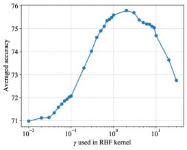
Refer to caption
Figure 9: The γ𝛾\gamma dependency of the RBF kernel performance.

F.1.3 Model specifications

We used kernel regression implemented in scikit-learn777https://scikit-learn.org/stable/modules/generated/sklearn.kernel_ridge.KernelRidge.html. To consider ridge-less situation, regularization strength is set to be 1.0×1081.0superscript1081.0\times 10^{-8}, a very small constant.

F.1.4 Computational costs

Since the training and inference algorithms of the kernel regression are common across different kernels, we analyze the computational cost of computing a single value in a gram matrix of the corresponding kernels in the following. The time complexity of the MLP-induced NTK is linear with respect to the layer depth, while that of the TNTK remains to be constant. Such a trend can be seen in the right panel of Figure 7. For the RBF kernel, the computational cost remains the same with respect to changes in hyperparameters, thus its trend is similar to the TNTK. In terms of the space complexity, when considering a multi-layered MLP, since it is not necessary to store all past calculation results in memory during the recursive computation, the MLP-induced NTK computation consumes a certain amount of memory regardless of the depth of the layers. Therefore, the memory usage is almost the same across the RBF kernel, TNTK, and MLP-induced NTK.

F.1.5 Computational resource

We used Ubuntu Linux (version: 4.15.0-117-generic) and ran all experiments on 2.20 GHz Intel Xeon E5-2698 CPU and 252252252 GB of memory.

F.2 Results

F.2.1 Statistical significance of the parameter dependency
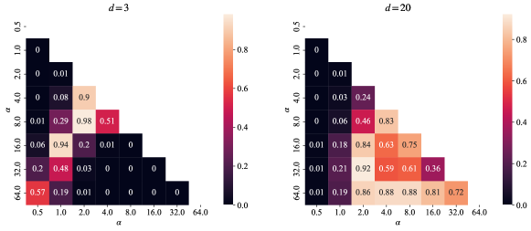
Refer to caption
Figure 10: P-values of the Wilcoxon signed rank test for different pairs of α𝛼\alpha.

A Wilcoxon signed rank test is conducted to check the statistical significance of the differences between different α𝛼\alpha. Figure 10 shows the p-values for the depth of 333 and 202020. As shown in Figure 7, when the tree is shallow, the accuracy started to deteriorate after around α=8.0𝛼8.0\alpha=8.0, but as the tree becomes deeper, the deterioration became less apparent. Therefore, statistically significantly different pairs for deep tress and shallow trees are different. When the tree is deep, large α𝛼\alpha shows a significant difference over those with small α𝛼\alpha. However, when the tree is shallow, the best performance is achieved with α𝛼\alpha of about 8.08.08.0, and if α𝛼\alpha is too large, the performance deteriorates predominantly.
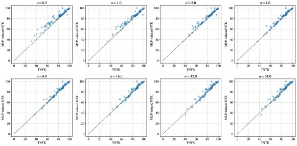
Refer to caption
Figure 11: Performance comparisons between the kernel regression with MLP-induced NTK and the TNTK on the UCI dataset.
Refer to caption
Figure 12: Performance comparisons between the kernel regression with RBF kernel and the TNTK on the UCI dataset.
Refer to caption
Figure 13: Pearson’s correlation coefficients with predicted values of the TNTK with different α𝛼\alpha.

F.2.2 Dataset-wise results

For each α𝛼\alpha, scatter-plots are shown in Figures 11 and 12. As shown in Figure 13, the correlation coefficients with the TNTK are likely to be higher for the MLP-induced NTK than for the RBF kernel. Tables 2, 3 and 4 are dataset-wise results of the comparison between the TNTK, the MLP-induced NTK, and the RBF kernel. For each α𝛼\alpha, depth is tuned for each dataset. In terms of the depth, the best performers from 111 to 292929 are compared with the TNTK and the MLP-induced NTK. For the RBF kernel, γ𝛾\gamma is tuned in each dataset from 303030 candidate values as described in Section F.1.2. Therefore, the number of tunable parameters is the same across all methods. All parameter-wise results are visualized in Figures 14 and 15.

name size α𝛼\alpha=0.5 α𝛼\alpha=1.0 α𝛼\alpha=2.0 α𝛼\alpha=4.0 α𝛼\alpha=8.0 α𝛼\alpha=16.0 α𝛼\alpha=32.0 α𝛼\alpha=64.0 MLP-NTK RBF
0 trains 10 87.500 87.500 87.500 87.500 87.500 87.500 87.500 87.500 100.000 87.500
1 balloons 16 87.500 100.000 93.750 87.500 87.500 87.500 87.500 87.500 100.000 93.750
2 lenses 24 87.500 87.500 87.500 87.500 87.500 87.500 87.500 87.500 87.500 87.500
3 lung-cancer 32 56.250 53.125 53.125 53.125 53.125 56.250 59.375 59.375 65.625 53.125
4 post-operative 90 63.636 64.773 67.045 69.318 69.318 68.182 68.182 69.318 69.318 56.818
5 pittsburg-bridges-SPAN 92 55.435 57.609 58.696 67.391 65.217 66.304 66.304 67.391 65.217 58.696
6 fertility 100 84.000 88.000 89.000 89.000 89.000 89.000 89.000 89.000 89.000 83.000
7 zoo 101 100.000 99.000 99.000 99.000 99.000 99.000 99.000 99.000 99.000 99.000
8 pittsburg-bridges-T-OR-D 102 81.000 84.000 87.000 89.000 89.000 89.000 88.000 88.000 87.000 89.000
9 pittsburg-bridges-REL-L 103 67.308 74.038 75.000 74.038 75.962 75.962 75.962 75.962 74.038 74.038
10 pittsburg-bridges-TYPE 105 57.692 59.615 64.423 66.346 66.346 66.346 66.346 65.385 68.269 59.615
11 molec-biol-promoter 106 90.385 88.462 87.500 87.500 87.500 87.500 87.500 87.500 90.385 88.462
12 pittsburg-bridges-MATERIAL 106 93.269 94.231 94.231 94.231 94.231 94.231 94.231 94.231 94.231 93.269
13 breast-tissue 106 65.385 68.269 67.308 70.192 72.115 72.115 75.000 74.038 69.231 71.154
14 α𝛼\alphacute-nephritis 120 100.000 100.000 100.000 100.000 100.000 100.000 100.000 100.000 100.000 100.000
15 α𝛼\alphacute-inflammation 120 100.000 100.000 100.000 100.000 100.000 100.000 100.000 100.000 100.000 100.000
16 heart-switzerland 123 37.097 43.548 48.387 47.581 50.000 44.355 44.355 44.355 47.581 37.903
17 echocardiogram 131 81.061 81.061 84.848 84.091 85.606 85.606 85.606 85.606 85.606 78.030
18 lymphography 148 88.514 88.514 88.514 88.514 87.838 87.162 86.486 86.486 88.514 86.486
19 iris 150 95.946 97.973 96.622 88.514 86.486 87.162 87.838 87.162 87.162 96.622
20 teaching 151 56.579 57.895 58.553 60.526 64.474 67.105 67.105 67.763 63.158 60.526
21 hepatitis 155 83.974 85.256 85.256 84.615 84.615 84.615 84.615 85.256 83.974 85.256
22 wine 178 98.864 99.432 98.864 98.864 98.864 98.295 98.295 97.727 99.432 98.295
23 planning 182 62.222 65.556 70.000 71.667 71.667 72.222 72.222 72.222 72.222 67.222
24 flags 194 52.083 53.646 53.646 53.125 53.646 53.125 53.125 53.125 53.646 49.479
25 parkinsons 195 93.878 94.388 92.857 93.367 92.857 92.857 93.367 93.367 93.878 95.408
26 breast-cancer-wisc-prog 198 82.143 83.673 83.673 83.673 83.673 83.673 83.673 83.673 85.204 78.571
27 heart-va 200 31.000 34.000 36.000 36.000 37.500 39.000 40.500 43.000 36.500 29.000
28 conn-bench-sonar-mines-rocks 208 86.538 86.538 87.019 86.538 86.538 86.538 86.538 86.538 87.981 87.500
29 seeds 210 90.865 93.750 93.269 91.827 92.308 92.308 91.827 91.827 96.154 95.673
Table 2: Comparison between TNTK and MLP-induced NTK for a half of the dataset (1/3).
name size α𝛼\alpha=0.5 α𝛼\alpha=1.0 α𝛼\alpha=2.0 α𝛼\alpha=4.0 α𝛼\alpha=8.0 α𝛼\alpha=16.0 α𝛼\alpha=32.0 α𝛼\alpha=64.0 MLP-NTK RBF
30 glass 214 60.849 67.453 70.755 70.755 71.698 71.698 71.226 71.226 70.283 69.811
31 statlog-heart 270 83.209 87.313 87.687 88.433 88.433 88.433 87.687 87.313 86.567 82.463
32 breast-cancer 286 64.789 67.254 69.718 70.423 72.887 74.648 75.000 75.000 71.831 65.845
33 heart-hungarian 294 83.219 83.904 84.247 84.589 85.616 85.274 85.274 85.274 85.616 82.877
34 heart-cleveland 303 55.263 58.224 58.882 59.211 59.539 58.553 59.211 59.539 57.895 53.618
35 haberman-survival 306 59.539 61.513 61.842 66.447 68.421 71.711 73.684 73.684 71.053 70.395
36 vertebral-column-2clases 310 69.805 77.273 78.571 80.844 82.792 84.091 84.091 82.792 83.117 81.494
37 vertebral-column-3clases 310 71.753 78.247 81.169 80.844 80.844 81.818 81.494 81.169 81.818 81.169
38 primary-tumor 330 47.561 50.305 52.134 53.049 52.744 50.610 50.305 50.000 52.134 45.427
39 ecoli 336 71.429 79.167 83.036 84.524 86.012 86.607 86.905 86.905 85.417 81.250
40 ionosphere 351 90.057 91.477 90.341 87.784 88.352 88.352 88.352 88.352 91.761 92.330
41 libras 360 82.778 81.389 80.556 80.833 81.111 80.833 80.833 80.833 83.889 85.278
42 dermatology 366 97.802 97.802 97.527 97.527 97.253 97.253 97.253 97.253 97.802 97.253
43 congressional-voting 435 61.697 61.697 61.927 61.927 61.927 61.697 61.697 61.697 61.697 62.156
44 α𝛼\alpharrhythmia 452 69.469 65.265 64.602 64.823 64.823 64.823 64.823 64.823 71.239 69.248
45 musk-1 476 89.076 89.076 89.076 89.286 89.286 89.076 89.076 89.076 89.706 90.756
46 cylinder-bands 512 79.883 78.125 78.125 78.320 78.516 78.320 78.320 78.320 80.273 79.688
47 low-res-spect 531 91.729 91.353 90.602 89.474 88.534 87.782 87.218 87.218 91.353 90.226
48 breast-cancer-wisc-diag 569 96.127 96.655 97.359 97.359 97.359 96.831 96.479 96.479 97.007 95.599
49 ilpd-indian-liver 583 64.897 69.521 70.719 72.260 71.062 71.747 72.603 72.603 71.918 70.377
50 synthetic-control 600 99.333 99.333 99.167 98.833 98.333 97.833 97.000 96.667 98.833 99.333
51 balance-scale 625 81.250 84.615 88.782 89.904 91.346 90.064 85.256 85.256 93.269 90.865
52 statlog-australian-credit 690 59.012 60.610 64.099 66.279 67.151 68.023 68.023 68.023 66.279 59.302
53 credit-approval 690 82.558 85.174 86.628 87.209 87.645 87.791 87.791 87.355 87.064 81.686
54 breast-cancer-wisc 699 96.286 97.286 97.857 97.857 98.000 98.000 98.000 98.000 98.000 96.714
55 blood 748 67.513 65.775 63.369 69.786 72.727 73.529 75.802 77.005 74.064 78.075
56 energy-y2 768 89.583 89.453 88.021 87.891 88.151 87.630 87.630 87.630 88.281 90.755
57 pima 768 68.229 70.182 71.354 73.307 76.042 76.302 77.083 76.693 75.000 69.661
58 energy-y1 768 93.750 93.620 93.229 90.495 90.234 90.104 90.234 90.234 92.708 96.484
59 statlog-vehicle 846 78.318 77.014 76.540 73.578 72.986 72.156 72.038 72.038 81.398 77.488
Table 3: Comparison between TNTK and MLP-induced NTK for a half of the dataset (2/3).
name size α𝛼\alpha=0.5 α𝛼\alpha=1.0 α𝛼\alpha=2.0 α𝛼\alpha=4.0 α𝛼\alpha=8.0 α𝛼\alpha=16.0 α𝛼\alpha=32.0 α𝛼\alpha=64.0 MLP-NTK RBF
60 oocytes_trisopterus_nucleus_2f 912 82.456 82.566 82.456 82.675 80.811 78.728 78.070 77.851 84.978 79.605
61 oocytes_trisopterus_states_5b 912 92.325 92.982 93.640 93.092 91.667 90.022 89.693 89.693 94.189 91.228
62 tic-tac-toe 958 99.268 99.163 99.268 99.268 99.268 99.268 99.268 99.268 98.640 100.000
63 mammographic 961 72.708 71.250 72.083 75.625 77.604 78.854 78.958 79.271 80.000 78.750
64 statlog-german-credit 1000 75.200 76.500 77.800 77.300 76.200 75.500 75.500 75.400 77.500 73.700
65 led-display 1000 72.400 72.300 72.600 72.500 72.300 72.500 72.300 72.500 72.900 73.000
66 oocytes_merluccius_nucleus_4d 1022 81.078 80.588 80.686 80.686 79.412 77.255 76.961 76.765 83.725 75.490
67 oocytes_merluccius_states_2f 1022 92.353 91.961 92.157 92.157 91.373 90.784 90.784 90.490 93.039 92.059
68 contrac 1473 40.082 44.293 47.147 50.068 51.155 52.038 52.514 51.155 50.272 43.207
69 yeast 1484 42.588 49.326 54.380 58.154 60.040 60.243 60.445 60.849 59.636 54.380
70 semeion 1593 93.719 93.467 93.405 93.467 93.467 93.467 93.467 93.405 96.168 95.603
71 wine-quality-red 1599 63.062 65.938 68.812 70.000 70.625 70.375 70.312 70.312 69.625 64.438
72 plant-texture 1599 83.812 81.812 79.438 77.938 77.688 77.625 77.750 77.625 86.125 85.625
73 plant-margin 1600 84.750 83.938 82.938 81.875 80.750 79.500 78.938 78.563 84.875 83.875
74 plant-shape 1600 64.812 63.562 62.438 60.375 58.312 57.062 56.375 55.937 66.250 68.000
75 car 1728 97.454 97.569 97.164 96.701 96.354 96.181 96.123 96.123 97.743 98.032
76 steel-plates 1941 76.289 77.320 77.938 77.423 77.062 76.753 76.598 76.495 78.351 75.103
77 cardiotocography-3clases 2126 92.232 92.514 92.043 91.902 91.949 91.855 91.996 91.855 93.173 92.043
78 cardiotocography-10clases 2126 80.838 82.957 82.250 80.744 79.896 79.896 79.661 79.614 84.181 79.143
79 titanic 2201 78.955 78.955 78.955 78.955 78.955 78.955 78.955 78.955 78.955 78.955
80 statlog-image 2310 96.360 96.967 97.097 96.750 96.231 95.927 95.884 95.624 97.660 96.404
81 ozone 2536 97.358 97.240 97.200 97.200 97.200 97.200 97.200 97.200 97.397 97.200
82 molec-biol-splice 3190 86.731 85.947 84.536 83.093 82.465 82.403 82.371 82.371 86.920 86.418
83 chess-krvkp 3196 99.124 98.905 98.655 97.872 96.902 95.526 95.307 95.307 99.406 98.999
84 α𝛼\alphabalone 4177 50.407 49.880 55.532 60.010 62.548 64.200 64.943 65.086 63.410 64.152
85 bank 4521 88.628 89.336 89.358 89.513 89.358 89.159 89.181 89.159 89.735 88.142
86 spambase 4601 91.478 91.174 92.435 90.652 93.130 89.630 91.478 93.348 94.913 90.652
87 wine-quality-white 4898 63.623 66.810 67.545 68.791 69.158 68.975 68.995 68.913 69.097 65.748
88 waveform-noise 5000 86.360 86.340 86.520 86.540 86.720 86.500 85.900 85.520 86.540 85.460
89 waveform 5000 85.440 85.780 86.300 86.500 86.660 86.700 86.740 86.520 86.340 84.640
Table 4: Comparison between TNTK and MLP-induced NTK for a half of the dataset (3/3).
Refer to caption
Figure 14: Dataset-wise comparison for a half of the dataset (1/2).
Refer to caption
Figure 15: Dataset-wise comparison for a half of the dataset (2/2).