Lifetime effects and satellites in the photoelectron spectrum of tungsten metal

Abstract

Tungsten is an important and versatile transition metal and has a firm place at the heart of many technologies. A popular experimental technique for the characterisation of tungsten and tungsten-based compounds is X-ray photoelectron spectroscopy (XPS), which enables the assessment of chemical states and electronic structure through the collection of core level and valence band spectra. However, in the case of metallic tungsten, open questions remain regarding the origin, nature, and position of satellite features that are prominent in the photoelectron spectrum. These satellites are a fingerprint of the electronic structure of the material and have not been thoroughly investigated, at times leading to their misinterpretation. The present work combines high-resolution soft and hard X-ray photoelectron spectroscopy (SXPS and HAXPES) with reflection electron energy loss spectroscopy (REELS) and a multi-tiered ab-initio theoretical approach, including density functional theory (DFT) and many-body perturbation theory (G0W0 and GW+C), to disentangle the complex set of experimentally observed satellite features attributed to the generation of plasmons and interband transitions. This combined experiment-theory strategy is able to uncover previously undocumented satellite features, improving our understanding of their direct relationship to tungsten’s electronic structure. Furthermore, it lays the groundwork for future studies into tungsten based mixed-metal systems and holds promise for the re-assessment of the photoelectron spectra of other transition and post-transition metals, where similar questions regarding satellite features remain.

I Introduction

Interest in tungsten (W) metal is seeing a resurgence owing to its high sputtering threshold, [1] low hydrogen retention, [2, 3] and high temperature resistance, [4] all of which make it extremely attractive as a plasma facing material in nuclear fusion reactors. [5, 6] Additionally, tungsten forms the base of many technologies in a range of industrial fields, with tungsten oxides being widely used for their electronic, photoabsorption, optical, and catalytic properties. [7, 8, 9, 10, 11] Tungsten-based alloys and intermetallic compounds find applications as diffusion barriers in metallisation schemes for semiconductor devices due to their chemical inertness towards the surrounding materials and high chemical blocking efficiency. [12, 13, 14, 15] The functionality and reliability of these materials is to a large extent governed by the electronic structure of the base metal. [16] Moreover, when characterising the properties of tungsten-based compounds, studies often necessitate comparison to those of tungsten metal to elucidate differences. Therefore, the investigation and accurate determination of the electronic structure of tungsten metal is highly relevant today and critical for the design of new materials and implementation of new tungsten-based technologies.

The characterisation of the electronic structure of metallic tungsten using both theoretical and experimental approaches has a long-standing history spanning many decades. The first calculations of the electronic band structure of tungsten were reported by Manning et al. in 1939. [17] Studies have followed continuously since then. [18, 19, 20, 21, 22, 23, 24, 25, 26] Most notably, Mattheiss et al. [18] provided the first theoretical study investigating the Fermi surface of tungsten using a non-relativistic approach, followed by Christensen et al., who expanded on this study by calculating the band structure using a relativistic augmented-plane-wave (APW) method coupling the theory results with experimentally obtained photoelectron spectra. [27, 28] More recently, theoretical investigations have transitioned from calculating tungsten’s band structure to more application-driven investigations into the interaction of molecules with tungsten surfaces, point defect studies, or the study of nanostructures. [29, 30, 31, 32, 33, 34] Several approaches have been used to calculate the projected density of states (PDOS) of tungsten, but these results have not yet been directly compared (with photoionisation cross section and broadening corrections) to high-resolution valence band spectra. [27, 20, 22, 26, 16] Beyond band structure features, the photoelectron spectrum also contains satellite peaks which arise from the additional excitation of a plasmon or electron-hole pair. To date, no theoretical study of satellites in tungsten has been reported. Such a treatment requires the use of many-body perturbation theory (MBPT), which has already shown promise for the determination of plasmon satellites in sodium and aluminium, [35], and silicon, [36, 37, 38], but also heavier transition metal compounds. [39, 40, 41]

Alongside these theoretical studies, several groups have experimentally explored the electronic structure, interfacial properties, and surface and bulk effects of tungsten, using a range of techniques, including soft angle-resolved photoelectron spectroscopy (ARPES), [42, 43, 44], hard X-ray ARPES (HARPES) [45], soft and hard X-ray photoelectron momentum microscopy [46, 47], inverse photoemission spectroscopy (IPES), [48] X-ray photoelectron spectroscopy (XPS), [49, 50, 51, 52, 53, 54] ultra-violet photoelectron spectroscopy (UPS), [55, 28, 49, 56, 57, 54] and synchrotron-based photoelectron spectroscopy. [58, 59, 60, 61, 62]

Despite the extensive existing body of both theoretical and experimental work on tungsten metal, there are still aspects of tungsten’s electronic structure and its influence on photoelectron spectra that have not been fully explored and understood. One particular aspect that warrants further investigation is the presence of plasmon satellites. The photoexcitation of electrons in metallic-like systems generates a final state effect, known as plasmon satellites, which appear as features on the higher binding energy (BE) side of the main ionisation peaks in photoelectron spectroscopy experiments, and originate from the coupling of the core hole and interaction of photoelectrons with conduction electrons. Such satellites present many challenges when analysing spectra and are rarely considered or in some cases misinterpreted as additional chemical states. Several experimental studies have explored plasmon satellites in the photoelectron spectra of metals, but these have been limited to first-row or noble “simple” metals, [63, 64, 65, 66, 67, 68] with a lack of investigation into the satellite structure of heavier transition metals, such as tungsten. Plasmon satellites have been confirmed in past electron energy loss spectroscopy studies on tungsten [69, 70], but to the best of our knowledge no XPS study has been reported that captures or discusses these satellites and their influence on the photoelectron spectrum.

Besides the presence of plasmon satellites, the core level peaks of tungsten recorded by photoelectron spectroscopy have their own inherent challenges. The two most frequently accessed core levels are the shallow W 4f (31-34 eV) and W 4d (240-260 eV). [52] The 4f spectrum is particularly difficult to analyse as the 4f peaks possess a narrow full-width at half maximum (FWHM), but also the 5p_3/2 core line lies in close proximity to the 4f_5/2 line, and so must be considered and included, if a peak-fit analysis is required. Additionally, if both the metal and tetravalent (IV) oxidation states are present, the 5p_3/2 metal core line overlaps with the 4f doublet peak of the W(IV) state. [71] The W 4d core level exhibits a large lifetime broadening, leading to a significant Lorentzian contribution to the line shape, which is often difficult to describe when peak fitting. Therefore, the presence of satellites and their lack of characterisation in tungsten photoelectron spectra, coupled with the complexity of the shallow core levels, form a strong motivation to revisit the photoelectron spectrum and electronic structure of tungsten.

The present work combines soft and hard X-ray photoelectron spectroscopy (SXPS and HAXPES) to study the satellite structure of key tungsten core levels, as well as providing high-resolution valence band spectra. HAXPES enables the exploration of bulk tungsten by minimising the pure surface nature of specific spectral features. In addition, it allows access to deeper core levels, which add complementary information to the common core states studied with SXPS and may offer a solution to the challenges associated with the interpretation of the complex W 4f and 4d core levels. Reflection electron energy loss spectroscopy (REELS) is used in parallel to directly determine the energy loss features of tungsten and to aid in the assignment of satellite features observed in photoelectron spectroscopy.

Given the complexity of the experimental spectra of tungsten, theoretical modelling is required to aid the interpretation of the spectral features, and this forms the primary motivation for the re-calculation of the electronic structure of tungsten. In order to fully analyse and interpret the complex electronic structure of tungsten, experiments are complemented with a multi-tiered theory approach. Density functional theory (DFT) [72, 73] is combined with MBPT within the GW and “GW plus cumulant” (GW+C) approaches. [74, 75, 37, 76] This allows the identification of specific observed spectral features arising from the electronic structure of tungsten, including the various satellite features. Additionally, given the interest in tungsten-based alloys in the semiconductor industry, linear-scaling DFT (LS-DFT) is used and compared to conventional cubic-scaling DFT. LS-DFT is able to model many-thousand atom systems by overcoming the computational cost limitations of cubic-scaling DFT, and thus is useful for the accurate description of disordered mixed-metal alloys in device systems in future studies. [77, 78]

II Experimental Methodology

A polycrystalline tungsten foil (99.95 at.% metal basis, 0.1 mm thick, Goodfellow Cambridge Ltd.) was used for the REELS, SXPS, and HAXPES measurements. Details regarding the ex- and in-situ preparation of the sample for the different measurements can be found in the Supplementary Information I. REELS measurements were conducted on a Thermo Scientific Nexsa XPS instrument, employing its flood gun as the electron source, with a beam energy of 1 keV and emission current of 5 $\mu$A. Back scattered electrons were measured using a 180^∘ hemispherical analyser in conjunction with a one-dimensional detector. A pass energy of 40 eV was used to collect the REELS data.

SXPS measurements were conducted on a Thermo K-Alpha XPS instrument, which operates with a monochromatised Al K$\alpha$ excitation source (1.4867 keV) and consists of a hemispherical analyser and two-dimensional detector. Measurements were conducted with a 400 $\mu$m elliptical spot size, 6 $\mu$A X-ray anode emission current, 30 $\mu$A flood gun emission current, and at a base pressure of 2$\times$10^-9 mbar. Survey, core level, and valence band spectra were collected with a pass energy of 200 eV, 20 eV, and 15 eV, respectively. HAXPES measurements were conducted on beamline I09 at the Diamond Light Source, UK. [79] A photon energy of 5.9267 keV (further referred to as 5.93 keV for simplicity) was selected using a double crystal Si (111) monochromator and an additional Si (004) channel-cut postmonochromator. The end station is equipped with a VG Scienta EW4000 electron analyser with a $\pm$28^∘ angular acceptance. All measurements were performed in grazing incidence geometry at angles below 5^∘ between the incoming X-ray beam and the sample surface. A pass energy of 200 eV was used for the collection of all spectra. The experimental resolution was evaluated by measuring the intrinsic Fermi edge of the tungsten sample and fitting the data with a Gaussian-broadened Fermi-Dirac distribution. From this the resolution of the SXPS and HAXPES measurements were determined to be 350 and 266 meV, respectively (see Supplementary Information II). The probing depth of the SXPS and HAXPES measurements is approximately three times the inelastic mean free path (IMFP) of the photoelectrons. The total IMFP of all electrons in tungsten was calculated using the TPP-2M formula resulting in values of 2.02 and 6.01 nm for the soft and hard X-ray excitation energies, respectively. [80]

III Computational Methodology

III.1 Density Functional Theory

When comparing DFT with valence XPS, a theoretical spectrum can be generated by calculating a partial density of states (PDOS), and applying appropriate photoionisation cross sections, as discussed below. The accuracy of the resulting spectrum thus depends on both the accuracy of the calculated energy bands, which is influenced by factors including the choice of exchange-correlation functional, basis set convergence, use of pseudopotentials and level of $k$-point sampling, and the details of the projection, i.e. choice of atomic orbitals and projection scheme. Since there is no unambiguous choice of either projection scheme or localized atomic basis, it is therefore important to consider the influence of different approaches. To this end, DFT calculations were performed with two different codes, the plane-wave Quantum Espresso code [81] and the wavelet-based BigDFT code [82], which use different basis sets, pseudopototentials, and projection schemes. For both sets of calculations the Perdew-Burke-Ernzerhof (PBE) exchange-correlation functional was employed. [83] For simplicity, the two approaches will be referred to by the basis set used for the calculations when discussing the results.

Quantum Espresso calculations were performed in the primitive unit cell, with a lattice parameter of 3.184 Å, with a 16 $\times$ 16$\times$ 16 k-point grid. In order to obtain a smooth density of states, the DFT eigenvalues were then interpolated onto a 64 $\times$ 64$\times$ 64 k-point grid. The PDOS was generated using a Löwdin population analysis-based approach. [84, 85] Further computational details, including the local orbitals used to perform the projection, are given in Supplementary Information III.

BigDFT calculations were performed using the linear scaling version of the code, [77, 78], since the localized and in-situ optimised atom-centred support function basis provides a natural and accurate approach for generating the PDOS, using a Mulliken-type projector [86] onto the support functions. [87, 88]. Furthermore, as previously discussed, the use of LS-DFT will be valuable for future studies of disordered mixed-metal systems, and it is thus important to compare LS-DFT results with experiment for bulk tungsten. As the first Brillouin Zone (BZ) is only sampled at the $\Gamma$-point in linear scaling BigDFT, $k$-point sampling is not available and so calculations were instead performed in a 12 $\times$ 12 $\times$ 12 body centered cubic (BCC) supercell with a side dimension of 38.804 Å (a = 3.234 Å), comprising 3456 atoms. For such a large supercell, $\Gamma$-point sampling was shown to be sufficient to reach total energy convergence. Additionally, 1458, 2000, and 2662 atom models were simulated (see Supplementary Information IV) to assess the supercell convergence. Further computational details are given in Supplementary Information III.

III.2 G0W0, and GW+C

Full frequency G0W0 calculations were carried out in BerkeleyGW [89] using the PBE eigenstates calculated using Quantum Espresso. The frequency-dependent dielectric matrix was calculated within the random phase approximation. Next, the frequency-dependent electronic self-energy was calculated for all eigenstates at all k-points in the symmetry-reduced k-point grid. We included the static remainder correction in the Coulomb hole term as described in Ref. [90]. Using the frequency dependent self energies, GW+C spectral functions were computed as described in Ref. [38]. As with the plane-wave DFT eigenvalues, the G0W0 eigenvalues and the GW+C spectral functions were interpolated onto a 64$\times$64$\times$64 k-point grid. Full details are provided in the Supplementary Information III.

The GW+C spectral functions from the BerkeleyGW calculations were also used to model the core level photoelectron spectra. The W 4f and W 5p electrons were explicitly included in the calculations. The calculated 4f and 5p spectral functions (at the $\Gamma$ point) were used to reconstruct the experimental 4f/5p core level spectrum, as follows: for each subshell, two copies of the calculated spectral function were added together, with one copy shifted by the atomic spin orbit splitting, determined from HAXPES measurements and weighted by the theoretical intensity ratio for the spin orbit doublet determined from the tabulated Scofield photoionisation cross section tabulated data [91]. The doublet peaks were then broadened to reflect the intrinsic lifetime broadening due to radiative recombination and Auger decay, as well as the experimental broadening. The resultant 4f and 5p simulated doublets were then scaled relative to each other using the Scofield cross sections and shifted accordingly to match the appearance of the experimental spectrum. The deeper core levels were not explicitly included in the calculations (they were contained within the pseudopotential). However, we note that the satellite structures of the different core levels are similar to each other (Fig. 6). Based on this observation, we have chosen to also use the calculated 4f spectral function to construct theoretical 3d and 4d spectra, using the same method as described above. We have recently used a similar approach for predicting core level line shapes in PdCoO₂. [41] A detailed explanation along with the values used to construct these simulated core level spectra can be found in the Supplementary Information V.

III.3 Comparison of Theory and Experiment

To provide a direct comparison between the theoretically calculated PDOS and the experimental valence band (VB) spectra, the PDOS was aligned to the calculated Fermi energy ($E_{F}$) from the respective calculations, and the VB spectra were aligned to the experimentally observed Fermi edge. Furthermore, the individual PDOS contributions require weighting according to their respective photoionisation cross sections ($\sigma_{i}$) at the photon energies used in the experiments. However, theoretical cross sections are only available for states which are occupied in the ground state of the atom. This presents a limitation in the case of tungsten, where the contribution from the p states is significant, and originates from mixing of the unoccupied 6p conduction band state. The 5p orbital is a shallow core level, at 38 eV above the Fermi energy, and is unlikely to contribute to states within the VB. Nevertheless, applying the theoretical cross sections for the 5p, 6s and 5d orbitals provides good agreement to experiment (see Supplementary Information VI). However, this approach is not well justified.

Mudd et al. [92] encountered a similar challenge, in the case of CdO, where the unoccupied Cd 5p state contributes to the valence p character. The Cd 5p orbital, much like the W 6p orbital, is unoccupied in the ground state of the atom, and so Mudd et al. approached the problem by multiplying the In 5p/In 5s cross section ratio to the cross section of the Cd 5s orbital to estimate the Cd 5p cross section. Indium was chosen as it is the first element to have an electron in the 5p orbital. Using this approach for tungsten, the ratio of Pb 6p/Pb 6s was multiplied with the W 6s cross section (values taken from Refs. [91, 93], but the resulting 6p cross section had almost negligible contribution to the simulated photoelectron spectrum (i.e. the sum of the weighted density of states), and did not result in a good agreement between experiment and theory (see Supplementary Information VI).

Another example is the case of metallic silver, where Panaccione et al. [94] attributed the “free electron-like character” of the unoccupied Ag 5p orbital to the valence p orbital character. In contrast to the method used by Mudd et al., Panaccione et al. applied a fitting procedure to optimise the weight of s, p and d contributions and therefore indirectly determine the 5p cross section. To apply this method to tungsten, the weighting factors of the s and d states were first constrained to the Scofield tabulated cross section values of the 6s and 5d states (see Supplementary Information VI) at the given excitation energy. [91] Then the p state weighting was determined by minimising the sum of the least squared difference between the simulated spectrum and experimental spectrum. This approach gave much better agreement (see Supplementary Information VI) to the experimental spectrum.

The comparison between the three approaches applied to the plane-wave DFT PDOS – (1) using the W 5p cross section (implemented using the Galore software package [95]), (2) determining the 6p cross section using cross sections of Pb, and (3) the “optimised” method outlined by Panaccione et al. are displayed in the Supplementary Information VI, with the “optimised” approach providing the most suitable weighting. When comparing theory to experiment in Section IV.3, the “optimised” W 6p state cross section (determined from optimising the G0W0 PDOS) and the Scofield W 6s and W 5d cross sections were used.

IV Results and Discussion

IV.1 REELS

A number of studies have used electron energy loss spectroscopies or optical techniques to probe the electronic excitations in tungsten. [96, 97, 98, 99, 100, 101, 69, 70, 102, 103, 104, 105, 106] These measurements provide a basis to help identify satellite features in the SXPS and HAXPES core level spectra, as will be discussed in Section IV.2, motivating the collection of a high-resolution REELS spectrum using a bulk-sensitive incident electron energy (see Fig. 1(a)). The first derivative of the energy loss intensity is displayed in Fig. 1(b) to aid with the identification of energy loss peaks and their energy positions. Prominent peaks are identified within five regions located between 10-54 eV, and labelled with letters (a-h) in Fig. 1(a). Table 1 lists the energy loss ($w$) positions of all identifiable peaks.

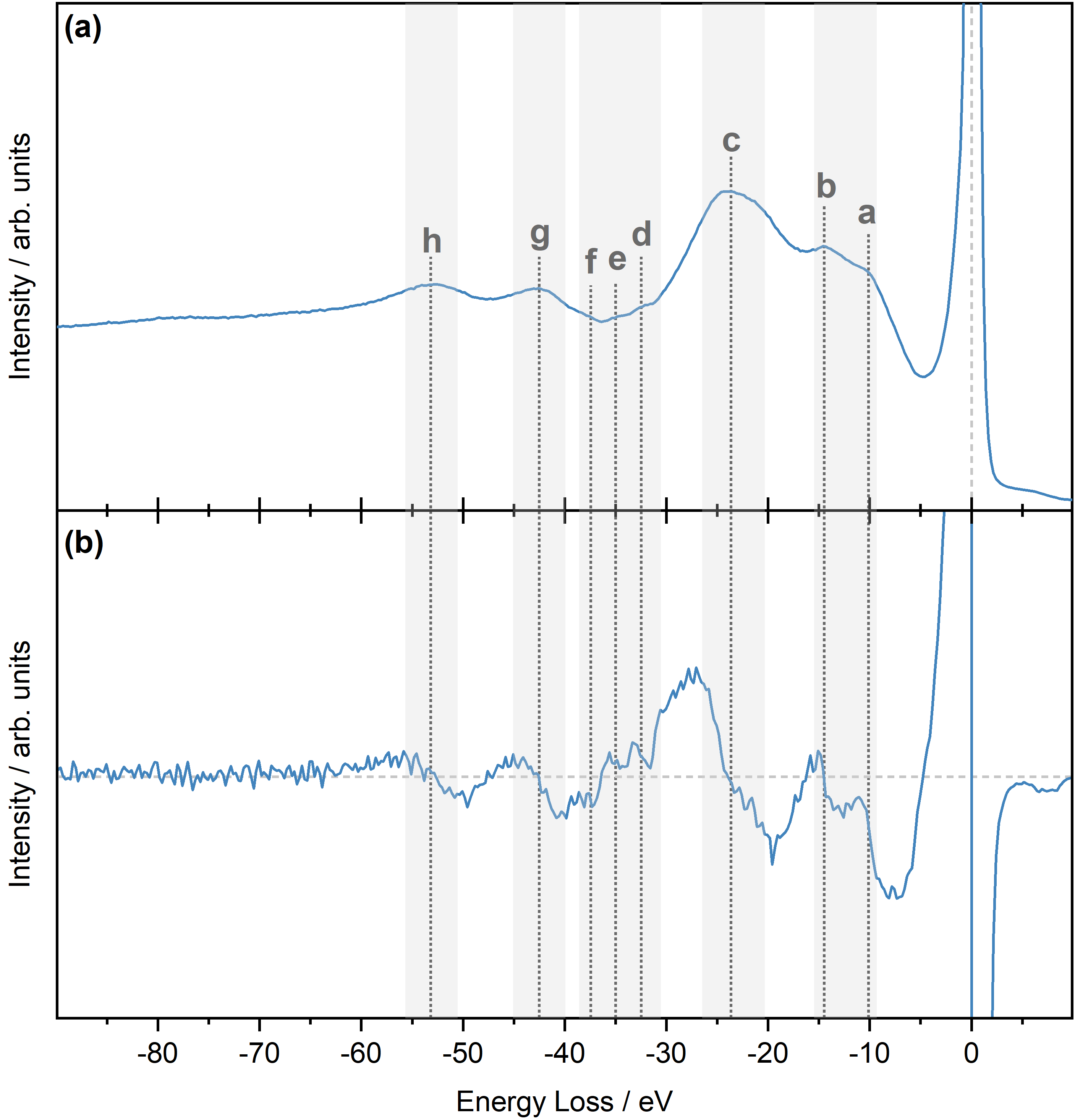
Figure 1: REELS spectrum of metallic tungsten. (a) Raw REELS spectrum, and (b) the first derivative of the REELS spectrum. Features of interest are labelled as a-h. The spectra are aligned so that the primary elastic peak is at 0 eV. The dotted horizontal line in (b) indicates y = 0.

Table 1: Energy loss regions and peak positions extracted from the recorded REELS spectrum as well as the feature notation used throughout.

Energy Loss Region / eV	Feature	w / eV
10-15	a	10.1
	b	14.5
21.8-25.5	c	23.7
30.5-39	d	32.5
	e	35.0
	f	37.5
40.0-45.5	g	42.5
50.5-55.8	h	53.2

Since the first reported electron energy loss measurements on tungsten by Harrower, [96] the origin of the observed loss peaks has been subject to continuous discussion but a definitive interpretation of the observed features remains outstanding. A good starting point for the interpretation of REELS data is to first determine the theoretical values of the surface and bulk plasmons using the Langmuir equation derived for a homogeneous electron gas. [107, 108] The theoretical bulk and surface plasmon energies of tungsten are estimated to be 22.8 and 16.2 eV, respectively, assuming six valence electrons per atom (5d⁴6s²).

The most intense feature c in Fig. 1 is located at an energy loss of 23.7 eV from the primary elastic peak at 0 eV. This is assigned as the bulk plasmon and is in good agreement with the theoretical bulk plasmon energy and values obtained in previous studies. [69, 70, 102] According to Weaver et al. the reason for the slight shift from the theoretical value is due to the existence of interband transitions close to the 25 eV region. [69]

Weaver, [69] Luscher, [70] and Avery [102] all observe that the surface plasmon of tungsten is much higher in energy than 16.2 eV, instead they assign a peak at approximately 20-21 eV to the surface plasmon. A shift from the theoretical value was also observed by Weaver et al. for other body centred cubic (BCC) transition metals (Nb, V, Ta, Mo), who attributed this observation to screening effects. [109, 110] The surface plasmon is difficult to observe in Fig. 1 as the incident electron energy is considerably higher than those of past studies, and therefore the collected data is dominated by the bulk plasmon. The region in which peak c resides does appear slightly asymmetric on the lower energy loss side and a secondary peak, perhaps the surface plasmon, may be present in this region. Avery also reported difficulty in resolving features in this energy loss region of tungsten using a 901 eV excitation energy. [102]

Two additional features, a and b are identified in the low-energy loss region at 10.1 eV and 14.5 eV, respectively. Several studies report peaks in this region for tungsten [70, 69, 102, 104], which are also found in other BCC transition metals [110, 111]. Shinar et al. summarises the discussion around the exact nature of these features [104], where Luscher et al. associate features below 18 eV to inter- or intra-band transitions [70], whereas Weaver et al. associate peaks in the region of 10 and 15 eV to a combination of overlapping surface and bulk plasmons. [69] More specifically, using optical measurements they identify two pairs of bulk and surface plasmons at energies of 10.0 and 9.7 eV (first pair) and 15.2 and 14.8 eV (second pair), respectively. Another possible explanation as to why these plasmons are found at lower energies is that the main plasmons are damped by interband transitions. [102] Alternatively, the lower energy bulk plasmon may only involve one group of electrons, with the main charge density from the d-like electrons omitted in this excitation. [110] Given the close proximity of the overlapping lower energy plasmons, they are often not resolved and appear as a single peak. These low energy plasmons are termed subsidiary plasmons or “lowered plasmons” and given that the observations by Weaver et al. appear well supported by others [112, 102, 104], we assign features a and b to these “lowered” plasmons.

The energy losses corresponding to features d, e and f closely match the core ionisation energies of W 4f_7/2, W 4f_5/2, and W 5p_3/2, respectively. A feature attributed to the W 5p_1/2 core level should appear at approximately 40 eV, but is difficult to observe in the spectrum as it overlaps with the more intense lower energy tail of feature g.

The high energy features g and h are reported at similar energy loss positions in previous studies. [96, 113, 97, 114, 99, 65, 70] Explanations regarding the origin of these features are only reported in studies by Tharp and Scheibner. [97, 114] They report peaks at energies of 43 eV and 53.5 eV for tungsten similar to our work, and conclude that as no combination of surface and bulk plasmon energy loss values (i.e. second order plasmon) could account for these loss features, they must be attributed to interband transitions between valence band orbitals and shallow core levels. In this work, the bulk plasmon energy loss value is 23.7 eV and therefore, if two plasmons combined to form a second order plasmon, a feature should occur at 47.4 eV (23.7$\times$2 = 47.4 eV), which is approximately 5 eV higher than feature h. Therefore, based on the data presented here a second order plasmon is unlikely and instead these features will be termed interband transitions in the following.

IV.2 Core Level Photoelectron Spectroscopy and Theory

The core level spectra of tungsten offer detailed insights into the electronic structure through the presence of extended satellite features. To disentangle and identify the complex satellite structure, this work combines a large number of deep and shallow core level spectra collected with both SXPS and HAXPES and calculated from theory. Survey spectra collected with SXPS and HAXPES are presented in the Supplementary Information VII. Additionally, the absolute binding energy (BE) of core level peaks, along with the full width at half maximum (FWHM), spin orbit splitting (SOS) separation, and relative BE separation between the main photoemission peak and corresponding satellite peaks, are listed in the Supplementary Information VIII. From the core level analysis, all core levels display asymmetric line shapes characteristic of metallic systems. [115, 116, 117]

IV.2.1 Shallow Core Levels

The two tungsten core levels most frequently accessed with XPS are W 4f and 4d, as they can be easily measured using standard Al and Mg K$\alpha$ laboratory X-ray sources. As mentioned earlier, the analysis of these core levels presents many challenges, which posses difficulties when chemical state and/or quantitative information is required. Here, high-resolution SXPS and HAXPES core level reference spectra of the shallow core levels are discussed. The information obtained from REELS is used to identify the origin and location of satellite features.

The BE positions of the W 4f and 4d core level peaks are in good agreement with past measurements. [118, 119, 120, 53, 121, 122, 60, 123, 52, 124] The W 4d core level (Fig. 2(a)) displays three satellite features, labelled S₁-S₃, which appear in identical positions in both SXPS and HAXPES spectra. Features S₁ and S₂ are located at 24.6 eV and 25.7 eV relative to the 4d_5/2 and 4d_3/2 photoemission peaks, respectively, and are bulk plasmon satellites. The broad and low intensity feature S₃ is detected at 53.6 eV relative to the 4d_5/2 photoionisation peak and based on the REELS assignments, originates from an interband transition. There is no significant difference in plasmon intensity or structure when comparing the SXPS and HAXPES spectra. This suggests that both techniques are more sensitive to the bulk plasmon, with the surface plasmon only weakly contributing to the spectra.

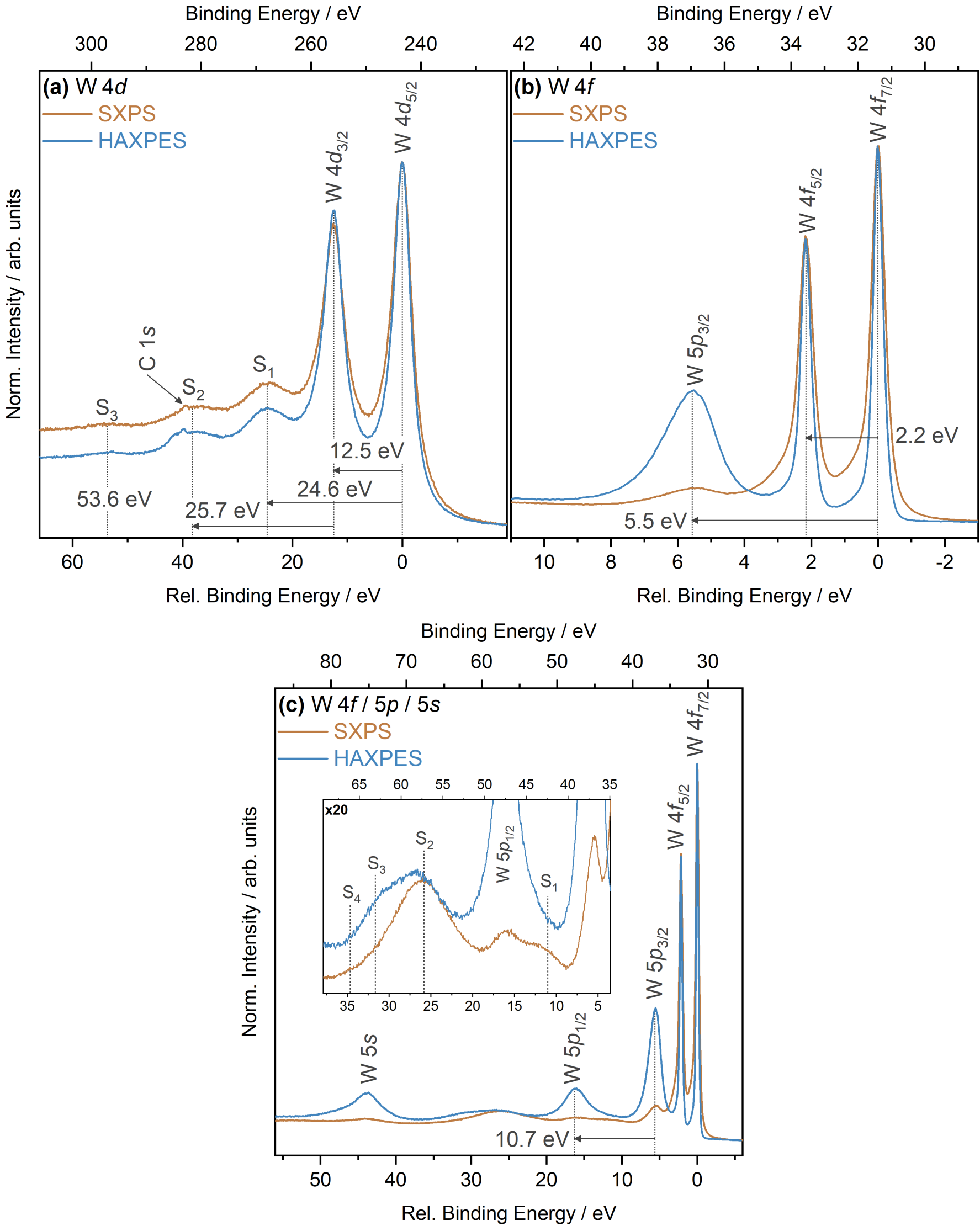
Figure 2: Shallow core level spectra collected with SXPS and HAXPES. (a) W 4d, (b) W 5p_3/2/4f, and (c) W 5s/5p/4f core levels. The inset in (c) shows a magnified view of the satellite region. Spectra are plotted on a relative BE scale, aligning the main photoionisation peak to 0 eV. The experimental binding energy scale is also displayed above each core level spectrum.

The rapid decay of photoionisation cross sections $\sigma$ at higher excitation energies ($\sigma$ $\propto$ E^-3) is often considered an intrinsic limitation of HAXPES measurements. However, in the case of the close lying W 5s/5p/4f core level the differences in the decay rates of cross sections between the orbitals can be used to aid interpretation of the spectra. A plot showing the photoionisation cross sections as a function of photon energy can be found in the Supplementary Information VI. In the HAXPES experiment the intensity of the shallow 5p and 5s core level peaks is enhanced compared to that of 4f. The 5p_3/2/4f_7/2 Scofield cross section ratio for tungsten is 0.15 at a photon energy of 1.4867 keV (Al K$\alpha$), and rises to 1.68 at 5.9267 keV. [91, 93] The enhancement in signal intensity is clear in the experimental data in Fig. 2(c). This enables the accurate determination of the SOS of the W 5p doublet peaks and was found to be 10.6 eV matching closely with the value reported by Sundberg et al. who also used HAXPES to determine the 5p SOS of tungsten. [125]

The satellite features in the shallow W 4f/5p/5s core levels are not as pronounced as those in the 4d core level. The inset in Fig. 2(c) highlights the satellite region between the 5p_3/2 and 5s core lines. Three satellite features appear in this region, as well as a higher BE low intensity satellite feature. Feature S₁ appears on the lower BE side of the 5p_1/2 peak at approximately 11.2 eV relative to the main 4f_7/2 core line. This feature leads to a slight asymmetric broadening of the 5p_1/2 core line in the HAXPES spectrum. However, the satellite is much clearer in the SXPS spectrum, owing to the reduced 5p_1/2 photoionisation cross section. To the best of our knowledge, this satellite has not been reported before and matches closely to the “lowered” plasmon loss energy peaks listed in Table 1. Two additional features, labelled S₂ and S₃ are observed at approximately 25.9 eV and 31.7 eV, respectively, relative to the 4f_7/2 core line. Feature S₂ can be assigned to the bulk plasmon and is linked to the plasmon generation by 4f electrons. Whilst feature S₂ appears in both the SXPS and HAXPES spectra, feature S₃ is only visually prominent in the HAXPES spectrum. The position of this feature relative to the 5p_3/2 is 25.2 eV, meaning that it is the bulk plasmon loss stemming from the 5p_3/2 electron. The large enhancement of its intensity in the HAXPES spectrum suggests that, much like core levels, the intensity of plasmon satellites has a dependence on the photoionisation cross sections. This further reinforces the benefit of using SXPS and HAXPES in parallel as the strategic tuning of photon energy allows for previously unidentified features to be enhanced. Lastly, feature S₄ is located at approximately 34.7 eV from the main photoionisation peak and has almost negligible intensity, making it difficult to observe, although it appears more prominent in the SXPS spectrum than the HAXPES. Its energy position suggests that it may be attributed to an interband transition stemming from the 4f and/or 5p core level electrons as the BE position occurs at an energy similar to the energy loss region of peaks d-e in the REELS spectrum.

In order to gain further insights into the satellite structures observed, the W 4d and W 4f/5p SXPS and HAXPES spectra are compared to GW+C simulated spectra (see Fig. 3). As for the 4d spectra, shown in Figs. 3(a) and (d), good agreement between experiment and theory is observed. The GW+C approach does remarkably well in predicting the relative intensity and binding energy positions of satellites S₁ and S₂. However, the third satellite at 53.6 eV is not captured by the calculation, likely owing to its relatively small intensity. Figs. 3(b) and (e) display the 4f and 5p_3/2 simulated core level spectra, where again good agreement between the relative intensities and broadening of the 4f doublet is found, especially for the SXPS case. In both the SXPS and HAXPES simulated spectra, the 5p_3/2 relative intensity is not as well described, which is due to the theoretical line widths being overestimated, [126] leading to a reduction in the peak height.

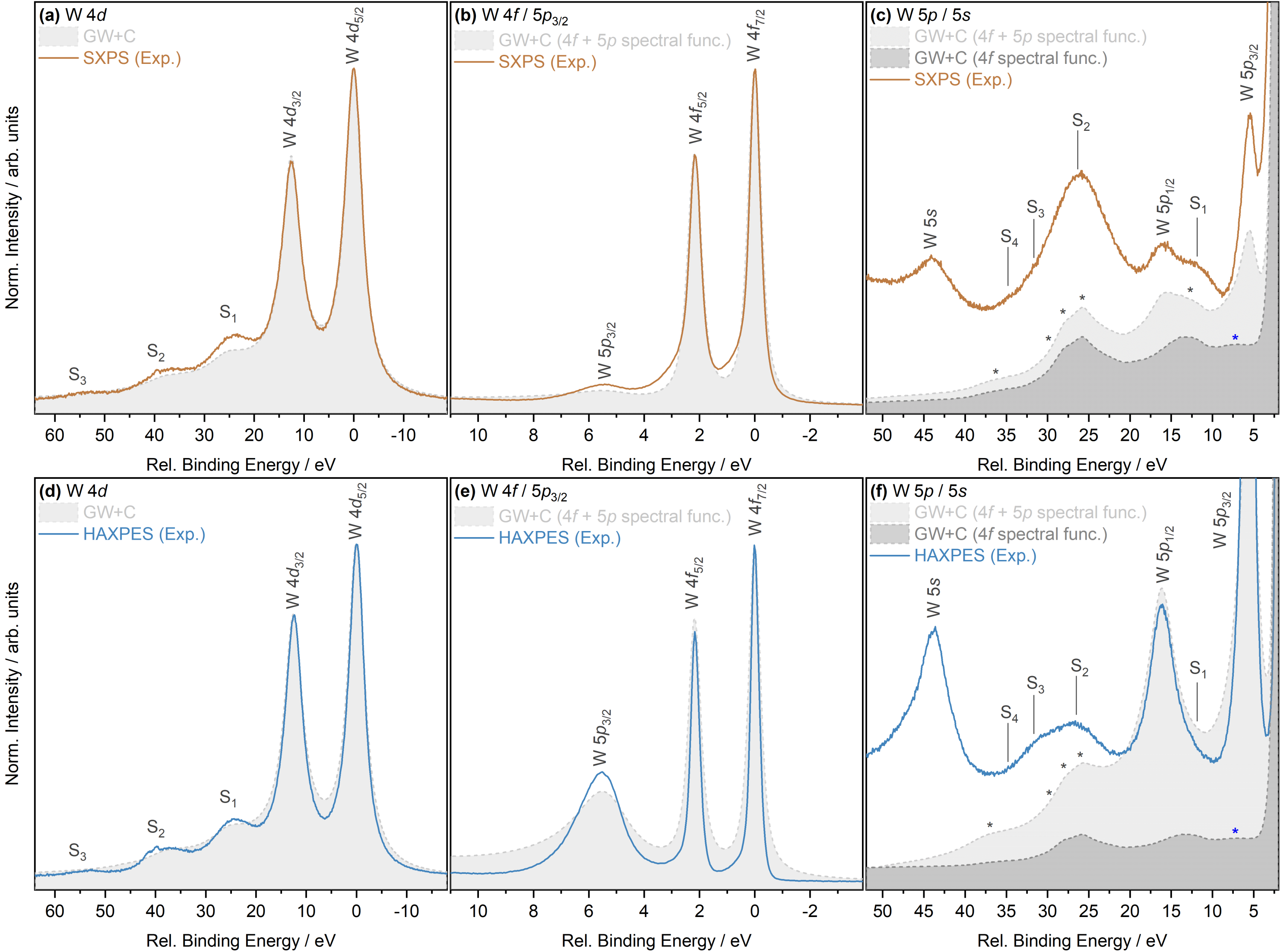
Figure 3: GW+C simulated spectra and experimental SXPS and HAXPES spectra of the shallow core levels. Going from left to right the W 4d, W 4f and W 5p_3/2, and enlarged W 5p/5s region core level spectra. The top row compares the GW+C simulated spectra to SXPS spectra, whereas the bottom row compares to HAXPES spectra. A Shirley-type background was removed from the experimental data to aid comparison to theory for the W 4d and W 4f/5p_3/2 spectra only. To aid with identifying the satellite structure in the 5p-5s region shown in (c) and (d), two simulated spectra are shown. One was calculated by using a combination of the 4f and 5p spectral function, with the other only using the 4f spectral function. Asterisks mark the satellite positions determined using GW+C. The black asterisks are shared between both the 4f+5p and 4f GW+C simulated spectra, whereas the blue asterisk is used to label the satellite feature only visible in the 4f GW+C simulated spectrum.

Figs. 3(c) and (f) show an enlarged view of the 5p and 5s region. Four satellite features can be observed in the SXPS spectra, and the simulated spectra determined from combining the 4f and 5p spectral functions match well, with the individual predicted satellite features marked with asterisks. Moving from lower to higher BE values, the GW+C approach predicts five satellites, appearing at 12.7 eV, 25.8 eV, 28.0 eV, 29.7 eV and 36.5 eV. The first predicted feature at 12.7 eV correlates well with S₁ and relates to the “lowered” plasmons found in the REELS spectrum. This feature is more apparent in Fig. 3(c) due to the reduced intensity of the 5p core levels with SXPS. Predicted features at 25.8 and 28.0 eV overlap and their separation ($\approx$2.2 eV) matches the SOS of the 4f core level. These features are attributed to bulk plasmons generated by the excitation of 4f_7/2 and 4f_5/2 core electrons, and contribute to the satellite S₂ seen in the experimental spectra. Overall, the GW+C predicted features describe the experimental observed satellite feature S₂ in both SXPS and HAXPES spectra well. S₃ at 30.9 eV, which is only clearly visible in the HAXPES spectrum due to cross section enhancement, and is attributed to a plasmon associated with the excitation of the 5p_3/2 electrons, is difficult to observe in the simulated spectra due to the limitations of the theoretical line widths used [126] and the resulting smearing of features. The last remaining predicted feature at 36.5 eV is very low in intensity, but can be assigned to the weak satellite S₄ visible in the SXPS spectrum. This satellite most likely arises from interband transitions between the 4f and conduction band states. It is expected to have higher intensity in the SXPS spectrum due to the enhanced photoionisation cross section compared to HAXPES.

In order to disentangle contributions from the 4f and 5p spectral functions Figs. 3(c) and (f) also display the simulated spectra determined using only the 4f spectral functions. In the 4f only simulation, all satellites previously described are present and an additional low intensity, low BE feature satellite is visible at approximately 7.3 eV from the 4f_7/2 peak. Whereas in the 4f and 5p simulation but also the experimental spectrum, this feature is difficult to observe as it sits underneath the 5p_3/2 core line. This 7.3 eV predicted feature does not appear in the REELS spectrum reported here, but Weaver et al. suggest that features within this region relate to interband transitions between valence and conduction band states. [69] The reason why this feature is not observed in our REELS spectrum is likely due to the employment of a high electron incident energy, which creates a large inelastic background, masking the low intensity feature.

IV.2.2 Evaluation of Core Level Line Widths

From the discussion presented so far it is clear that the intrinsic complexity of the shallow core lines, both in metallic tungsten and exacerbated when oxide and other compound states are present, complicates analysis. Therefore, a clear motivation exists to explore other core levels where these constraints are not present and hard X-rays can be used to unlock additional higher energy core levels.

An important aspect when combining core level spectra of different orbital natures and binding energies is the difference in lifetime broadening. The ideal alternative core level to analyse would be well separated from other neighbouring core levels, and has a natural line width similar to that of the W 4f core level, as this is narrow enough to resolve chemical shifts. It is important to remember, that core level line widths in XPS have both a Lorentzian and Gaussian component, with the former attributed to lifetime $\tau$ broadening effects in response to the creation of a core hole during the photoemission process and the latter attributed to non-lifetime effects (e.g. instrumental factors, temperature, phonon broadening etc.). The Lorentzian contribution to the line shape is given by,

$$\centering I(E)=I(E_{0})\frac{\Gamma^{2}}{(E-E_{0})^{2}+\Gamma^{2}}\textrm{,}\@add@centering$$ (1)

where $I$ is the spectral intensity at a given energy $E$, $E_{0}$ is the centroid energy of the Lorentzian peak, and $2\Gamma$ is the natural line width (e.g. core hole lifetime broadening), with $\Gamma$ given by

$$\centering\Gamma=\hbar/\tau=(6.582\times 10^{-16}~{}eV{\cdot}s)/\tau\textrm{.}\@add@centering$$ (2)

Fig. 4 compares the measured FWHMs of all core levels using both SXPS and HAXPES to the theoretical natural line widths reported by Perkins et al., [126] which include the sum of both radiative and non-radiative line widths, along with line widths determined from the comparison of available experimental and theoretical data by Campbell et al., which they define as “recommended line widths”. [127] The core levels vary substantially in their line widths with the 3s core level having the largest (16.5 eV) and the 4f having the smallest (0.4 eV), both determined from the HAXPES measurements. The main trend observed is that with increasing angular momentum (i.e. going from s to d orbitals) the natural line width decreases (e.g. $\Gamma$(3s)$>$ $\Gamma$(3p_1/2) $>$ $\Gamma$(3p_3/2) $>$ $\Gamma$(3d_3/2) $>$ $\Gamma$(3d_5/2)). This can be attributed to a reduction in the Coster-Kronig-Auger decay. [128] The measured shallow (4f-4d) core level line widths are in better agreement with the recommended line widths, whereas the deeper (3s-3d) core levels show a better agreement with the theoretical values. Campbell et al. note a scarcity of available data for the deeper core levels of elements above Z = 55, with only X-ray emission spectroscopy (XES) data available rather than XPS. Additionally, the SXPS recorded line widths for the 4f and 4d core lines are broader than the HAXPES recorded line widths due to the better energy resolution of HAXPES. Due to the low intensity of the 5p and 5s core lines in the SXPS spectra (as will be shown in Section IV.2.1) the accurate determination of their FWHM was not possible. Fuggle et al. suggest that the differences are due to other non lifetime-broadening effects. [128] Whereas Ohno et al. attribute certain discrepancies due to the theory approach taken by Perkins et al., suggesting the many-body-theory approach is necessary to offer better line width prediction to the experimental results. [129, 128]

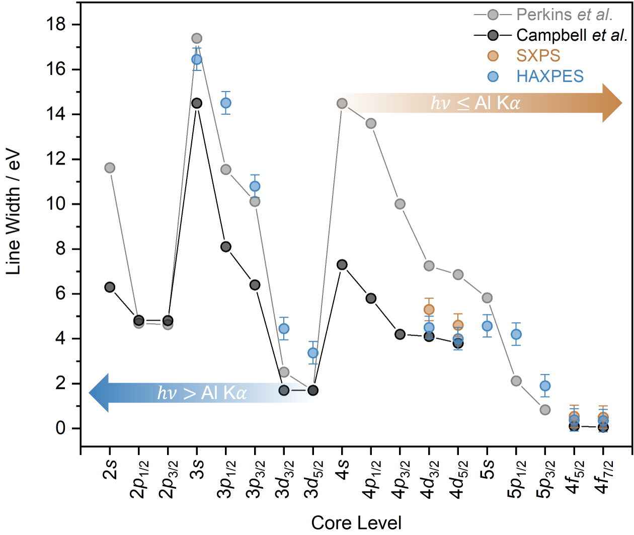
Figure 4: Comparison of the total core line widths of SXPS and HAXPES data with reported natural line-width values from Refs. [126, 127]. The W 5p and W 5s core level line widths are not reported by Campbell et al. and Perkins et al. do not calculate the W 4f line widths. All core levels up to and including the W 4s can be accessed with the Al K$\alpha$ photon energy, whereas to access deeper core levels (3d and above), a photon energy higher than Al K$\alpha$ is required.

From the HAXPES measurements, a FWHM of 3.4 eV for the W 3d_5/2 core line and a large 3d SOS of 62.1 eV are found, both of which are sufficient to allow for chemical shifts to be resolved. Additionally, Fig. 4 shows that its natural line width and therefore Lorentzian contribution is lower than that of the 4d core lines, and therefore is advantageous from an analytical perspective. Based on this information, the 3d core level can be considered as an alternative to the shallow 4d and 4f core levels and can be used to provide additional complimentary information from a different depth perspective.

IV.2.3 Deep Core Levels

The need to access deeper core levels for tungsten has not seen as much interest compared to titanium and silicon, where the Ti 1s and Si 1s core level is frequently accessed with HAXPES in favour of the Ti 2p and Si 2p core levels, as analysis is more straightforward due to the lack of impeding satellite structures, the higher photoionisation cross sections, and the absence of SOS effects to consider. [130, 131, 132] However, in light of the observation that the 3d core level may offer complimentary information to the commonly used shallow core levels, there is clear motivation to explore deeper core lines. Given the current popularity of HAXPES, there are also greater opportunities to conduct such experiments. [133] Therefore, the following discussion reports the first in-depth description of the deep core levels of tungsten metal collected with HAXPES.

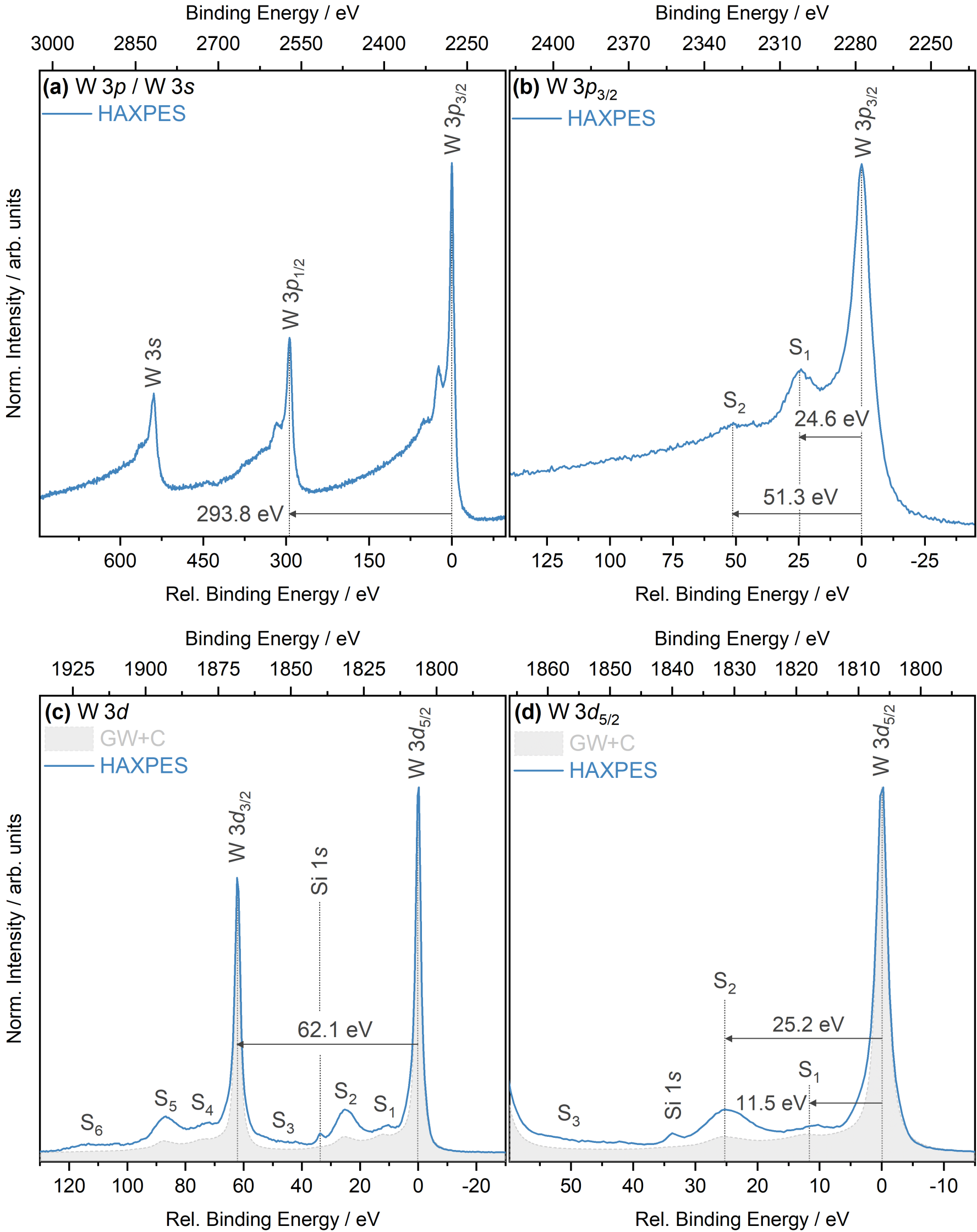
Figure 5: Core level spectra from HAXPES experiments and theoretical GW+C results for W 3d. (a) W 3p and W 3s, (b) W 3p_3/2, (c) W 3d, and (d) W 3d_3/2 core levels. Spectra are plotted on a relative BE scale, aligning the main photoionisation peak to 0 eV. The experimental binding energy scale is also displayed above each core level spectrum. The Si 1s core line appearing in the W 3d core level originated from the ex-situ sample preparation. (c) and (d) also show the comparison between the HAXPES W 3d core level spectrum and the GW+C simulated spectrum. A Shirley-type background was removed from the experimental spectrum and both the simulated and experimental spectra were normalised to the maximum peak intensity to aid with the comparison.

Fig. 5 displays the W 3p/3s, W 3p_3/2, W 3d and W 3d_5/2 core levels, which are only accessible using excitation energies above those of conventional soft X-ray laboratory sources. They display a complex satellite structure with large decaying backgrounds on the higher BE side of the main photoionisation peaks. To the best of our knowledge, there have only been two reported studies on the W 3d core level but none on the W 3s or W 3p core levels of tungsten metal. Wagner [134] appears to be the first to access the 3d_5/2 core line using a Au M$\alpha$ (2.123 keV) photon source, reporting a BE position of 1807.6 eV. However, no spectra were displayed in this study. More recently, Sundberg et al. accessed the 3d core level using HAXPES ($h\nu$ = 3 and 6 keV), reporting a BE position of the 3d doublet core lines of 1806.8 eV and 1868.9 eV. [125] Sundberg et al. only show the 3d_5/2 core line, and satellite features were not captured.

The BE positions of the 3d_5/2 and 3d_3/2 core level peaks observed in the current HAXPES experiment are 1806.3 eV and 1868.4 eV, respectively, with a SOS of 62.1 eV, matching closely with the values reported by Sundberg et al. Additionally, the BE position of the 3s, 3p_1/2 and 3p_3/2 core lines are 2817.3 eV, 2571.3 eV, and 2277.5 eV, respectively, with the 3p doublet having a SOS of 293.8 eV. The 3p_3/2 core level, displayed in Fig. 5(b), displays two satellite features located at 24.6 eV (S₁) and 51.3 eV (S₂) relative to the main photoionisation peak, and these features are mirrored by the 3p_1/2 spin component and also the 3s core level. To identify the origin of these satellites, comparison to the REELS data is helpful. The satellite features occur at similar positions to the energy loss values of features c and h (see Fig. 1). Following the assignments made for the REELS data, S₁ corresponds to the bulk plasmon and S₂ to an interband transition. The small differences in the BE positions of the features compared to the reported energy loss values in the REELS measurement can be attributed to the differences in the underlying excitation mechanisms between the two techniques. Plasmon satellites in photoemission experiments differ from plasmon-related features in electron energy loss experiments as they contain both intrinsic (due to photo-excitation) and extrinsic (electron scattering during transport to surface) plasmon losses, whereas energy loss experiments only contain the latter. [66, 135] Consequently, this can lead to a difference in intensity of these features, which can influence the accurate determination of their positions. Additionally, lifetime broadening effects in SXPS/HAXPES can impede the accurate determination of weak satellite features that lie close to the main photoemission peak.

The W 3d core level displayed in Fig. 5(c) displays six satellite features (S₁-S₆), shared equally and mirrored by each spin component (S₁ = S₄, S₂ = S₅, S₃ = S₆). Satellite features S₁ and S₂ in the 3d_5/2 core level region, shown in Fig. 5(d), appear at relative BE positions of 11.5 eV and 25.2 eV, respectively. S₂ and S₅ are the most intense satellite features and by using the previous assignments in REELS are assigned to the bulk plasmon. Features S₁ and S₄ appear at a similar position to the energy loss position of peak a in the REELS spectrum and therefore are attributed to a subsidiary plasmon. Whilst S₆ in the 3d_3/2 region is clearly observed, the mirrored feature S₃ is hard to distinguish due to the impeding lower BE tail of the 3d_3/2 peak. S₆ occurs at ca. 52.2 eV relative to the 3d_3/2 peak, matching closely to the second satellite feature in the 3p_3/2 core level, and are therefore considered to be an interband transition.

As for the shallow core levels, theoretical GW+C results were used to gain a better understanding of the complex satellite features observed. Fig. 5(c) and (d) displays the simulated W 3d core level, calculated using GW+C, and provides a direct comparison to the HAXPES data. Good agreement is observed between theory and experiment, with the core level line widths, line shape, and relative intensities being well reproduced. This suggests that both the applied Scofield photoionisation cross sections [91] and recommended line width values determined by Campbell et al. [127] work well for the case of tungsten.

Moreover, the use of the 4f spectral function to simulate this deep 3d core level is effective and shows that this approach could be used to simulate deep core levels for other metallic elements. In terms of the prediction of the satellite peaks, the GW+C approach is able to describe the first two satellite features. The satellites are located at 11.5 eV and 25.2 eV in the experiment, which agrees well with the theory positions of 12.5 eV and 25.3 eV. The second satellite is under-predicted in intensity in the simulated GW+C spectrum relative to the experimental spectrum. As mentioned above, plasmons are classified into either intrinsic or extrinsic categories, with both contributing to the experimental spectrum. However, GW+C only describes the intrinsic losses, which is why a reduction in signal intensity is observed. The third satellite feature (S₃, S₆) does not appear clearly in the GW+C calculation, similar to the case of the 4d simulated spectra (Figs. 3(a) and (d)) and again is most likely due to its vanishingly small intensity relative to the background.

IV.2.4 Comparison of Core Level Satellites

When comparing all core level spectra, similarities in their satellite features become clear. This is expected, as based on the above discussion, these features are a fingerprint of the intrinsic electronic structure of tungsten. Fig. 6 shows the comparison between the W 3p_3/2, W 3d_5/2, and W 4d core level HAXPES spectra. It is strikingly clear that all core level spectra (including the shallow W 4f/5p core level) share the same bulk plasmon satellite feature located at ca. 25 eV from the main photoionisation peak. Moreover, 3p_3/2 and 4d share the same low intensity satellite at  53.6 eV. The 3d_5/2 spectrum on the other hand displays a low intensity satellite at 11.5 eV, which is also present on the lower BE side of the 5p_1/2 core line (See Fig. 2(c)). Due to the SOS of the 4d core level, this satellite feature will appear under the 4d_3/2 core line, which is why it has never been observed. Additionally, it will also fall under the higher BE tail of the 3p_3/2 core line. However, given the low intensity of the satellite observed in the 3d core level, the presence of the satellite in the 4d core level will most likely not need to be considered during peak-fit analysis of the region. Likewise, given the presence of the 53.6 eV satellite in the 4d and 3p_3/2 core level regions, one can assume it is also present in the 3d_5/2 region, but due to its low intensity and close proximity to the 3d_3/2 core line it is smeared out.

Uncovering hidden satellite feature such as the ones discussed here, highlights the benefit of using both HAXPES and SXPS to understand the detailed satellite structures in core level spectra. A similar approach was used by Woicik et al., who discovered the appearance of a low intensity 5 eV satellite hidden underneath the Ti 2p_1/2 core line of SrTiO₃ by comparing the spectrum to the deeper Ti 1s core level. [136]

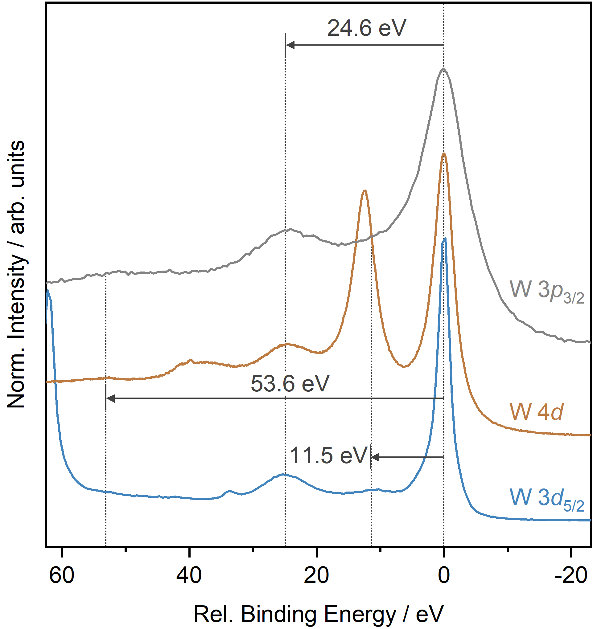
Figure 6: W 3p_3/2, W 4d, and W 3d_5/2 core level HAXPES spectra. Spectra are offset vertically, normalised to their maximum intensity, and aligned relative to the main photoionisation peak.

IV.3 Valence Electronic Structure

The information on the electronic structure gained from REELS and core level PES can be further extended by considering the valence electronic structure of tungsten. Several studies report the valence band spectrum of tungsten metal, predominantly focusing on PES using soft or ultra-violet photon energies, constraining the measurements to the sample surface. [49, 53, 52] Additionally, to date, no study has used HAXPES to capture a bulk valence band spectrum of tungsten that can be directly compared to theory. To address these limitations, high resolution valence band spectra with improved signal-to-noise ratio were obtained using both SXPS and HAXPES. Fig. 7 displays the collected valence band spectra and shows that the same features are present with both SXPS and HAXPES, and appear in near identical BE positions, which is expected for a metallic system. The subtle differences observed between the SXPS and HAXPES spectra are due to a combination of different energy resolution as well as differences in photoionisation cross sections.

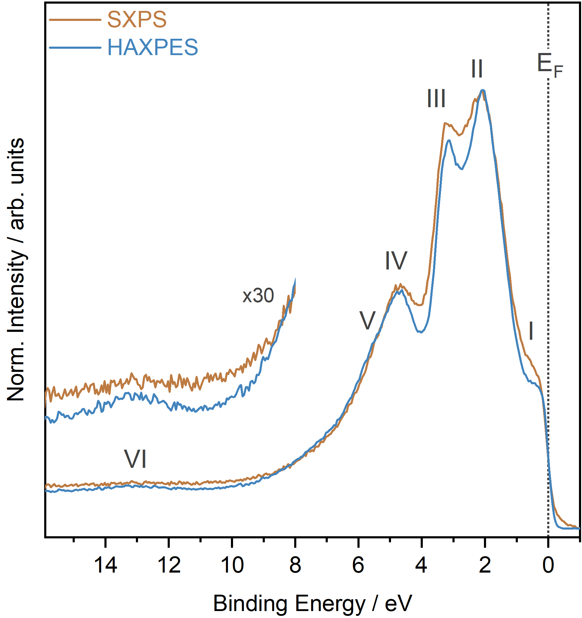
Figure 7: High resolution SXPS and HAXPES valence band spectra. Spectra are normalised to the maximum intensity after the removal of a constant linear background. The inset shows a $\times$30 magnification of feature VI plotted on the same x-axis scale.

Six key features are identified and labelled with Roman numerals – I, II, III, IV, V and VI – located at approximately 0.4 eV, 2.0 eV, 3.2 eV, 4.7 eV, 5.5 eV and 13.0 eV, respectively. The general shape of the valence band SXP spectrum is in good agreement with previous studies. [49, 53, 137, 52] This work is able to present a much higher resolution spectrum, resolving features II and III, where previous studies fail. [49, 52] The BE positions of features I-IV match closely to those presented by Hussain et al. who reported similar features at 0.6  eV, 2.3 eV, 3.2 eV and 4.8 eV using angle-resolved PES ($h\nu$ = Al K$\alpha$). [42] Feature V is more apparent in the HAXPES spectrum due to the subtle difference in cross sections between the 5d and 6p states.

Feature VI has not been observed to date. It appears close to features a and b reported in the REELS spectrum, which are attributed to the “lowered” plasmon losses. Feature VI is visible in both SXPS and HAXPES spectra, excluding a pure surface phenomenon. These observations give weight to the argument that this feature is an intrinsic part of the electronic structure of tungsten. A similar feature is also observed above the valence band of other BCC transition metals, [138, 139] which exhibit such “lowered” plasmons, however, this feature is never discussed. [109, 110] A similar observation was shared by Ławniczak-Jabłońska et al. who highlighted the presence of a low intensity valence band feature at 12 eV for molybdenum, much like feature VI in our spectra for tungsten. [140] They attribute the feature to an energy loss associated with an interband transition, which again further reinforces the assumption made earlier that feature VI is intrinsic to the electronic structure of tungsten and is due to what Weaver et al. states is a “lowered” plasmon loss.

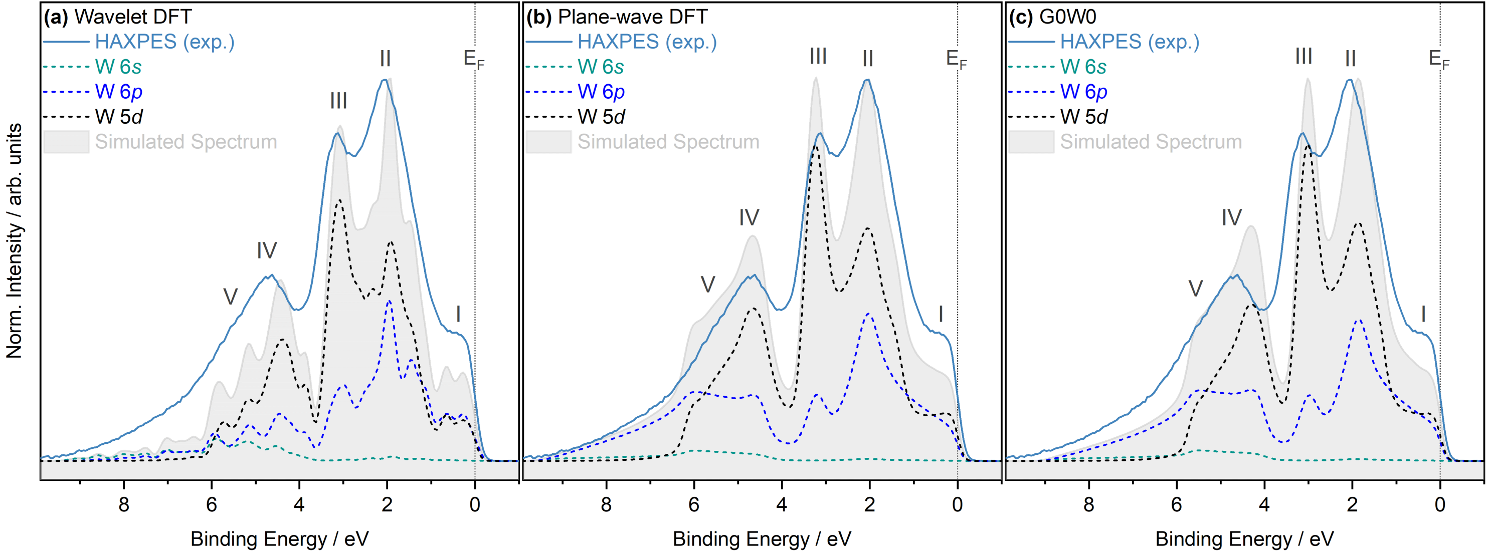
Figure 8: Comparison of simulated PDOS spectra calculated using DFT and G0W0 approaches with the HAXPES valence band spectra, including the comparison with (a) DFT using a wavelet basis set, (b) DFT using a plane-wave basis set, and (c) G0W0. The contributions to all PDOS spectra displayed are photoionisation cross section weighted using the “optimised” method outlined in Section III.3. A Shirley-type background was removed from the experimental spectrum to allow direct comparison to the theory. The PDOS contributions have also been suitably broadened to match the experimental broadening. Simulated Spectrum refers to the sum of the weighted PDOS. See Supplementary Information IX and X for the G0W0 unweighted PDOS and comparison of PDOS to the SXPS collected valence band spectrum, respectively.

Fig. 8 displays the calculated PDOS from both DFT approaches (using the wavelet and plane-wave basis sets) along with the G0W0 approach, and compares them to the experimental HAXPES valence band spectrum. The PDOS shown have been weighted using the Scofield W 5d and W 6s values at the given photon energy as well as the W 6p cross section determined using the “optimised” approach. All three theory approaches are in good agreement with the experimental result, clearly identifying all key features and their relative energy positions. The wavelet DFT approach (i.e. using LS-DFT) shows remarkable similarity to the plane-wave DFT approach (i.e. using conventional cubic-scaling DFT). However, the plane-wave DFT is smoother, which is also the case in the unweighted total densities of states (TDOS) (see Supplementary Information XI). Additional calculations were performed to assess the influence of both the lattice parameter and the pseudopotential choice, including whether or not the 5s and 5p states are included in the core or treated as valence states. The PDOS was found to be insensitive to both of these parameters, while spin orbit coupling was also found to have little influence. Thus, the differences between the TDOS for the two DFT approaches can be attributed to the smaller effective $k$-point sampling of the wavelet-based results. The strong effect of the choice of $k$-point sampling (or equivalently, supercell size) can be clearly seen in the Supplementary Information IV, where the calculated PDOS are presented for different supercell sizes. Due to the high computational cost, 3456 atoms was the largest system attempted, and although it appears close to convergence it could be interesting to consider larger supercells in future work.

Aside from the differences coming from the TDOS, the plane-wave DFT approach, shown in Fig. 7(b) projects a greater contribution from the 6p states between 6-9 eV, whereas the projection from the wavelet DFT approach (Fig. 7(a)) shows that the contributions from all states is almost minimised in this region. Referring again to the unweighted PDOS, the two DFT approaches show some difference in the relative contributions coming from both the 6s and 6p states below 4 eV, while the contribution arising from the 5d states is similar in both approaches. Upon applying the photoionisation cross sections, the stronger 6p-contribution in the plane-wave projection leads to higher relative peak heights in this region, while in the wavelet case the larger 6s-contribution is lost due to the smaller 6s cross section, leading to smaller relative peak heights. In other words, the differences between the two approaches below 4 eV are solely due to difference in the TDOS, i.e. resulting from the different $k$-point sampling, while the differences above 4 eV arise due to both the differences in the TDOS and in the projection scheme. Nonetheless, both DFT approaches give a good description of the experimental results, thereby highlighting the viability of using LS-DFT for the modelling of disordered metal alloy systems in large supercells. Whereas, comparing the plane-wave DFT PDOS to the G0W0 PDOS minimal differences are observed in the shape of the projection, with the only difference being that the G0W0 predicts a narrower band width. The overestimation of the band width from DFT calculations on metallic systems is a well known problem and is often a motivation for using G0W0. [141, 142]

The theory reflects the expected electronic structure with spatially localised 5d states providing the majority contribution to the valence band and free-electron like 6sp bands only giving a small contribution. Feature I is shown to arise from a mixing of the 6p and 5d states with both showing an equal contribution. Similarly, features II and III also arise from a mixing of 5d and 6p states, however, the 5d states dominate, especially for feature III. Feature IV also arises predominantly from mixing of the 5d states with 6p states with a small contribution from 6s states. This is also the case for feature V, which appears as a distinct shoulder on feature IV, which has a marginally higher contribution from s states.

All three theory approaches match the BE positions of the higher BE region (IV and V) well, but struggle to accurately describe the overall shape of the valence band in this region. Such discrepancies between DFT and photoelectron spectroscopy (PES) have been noted by others, [143, 144, 94] who have put forward two possible reasons – firstly the necessity of approximating exact exchange and correlation potentials, and secondly, the fundamental difference between DFT and PES, in that DFT is only considering the ground state, whereas PES reflects additional final state effects. For these reasons, the inclusion of self-energy corrections (i.e. G0W0 and GW+C) are typically needed to generate an improved comparison of theory to experiment. Therefore, the GW+C approach was used, with the result displayed in Fig. 9, which clearly provides a better agreement with the experimental spectra, especially in capturing the shape of the region around features IV and V. The GW+C PDOS curves that have been constructed from the calculated spectral functions contain the effects of lifetime broadening as well as photoemission satellites. In contrast, the DFT and G0W0 PDOS curves do not contain these effects. The ability of the GW+C method to more accurately predict the shapes of features IV and V in the experimental spectrum indicates that lifetime broadening has a significant influence on the appearance of these peaks.

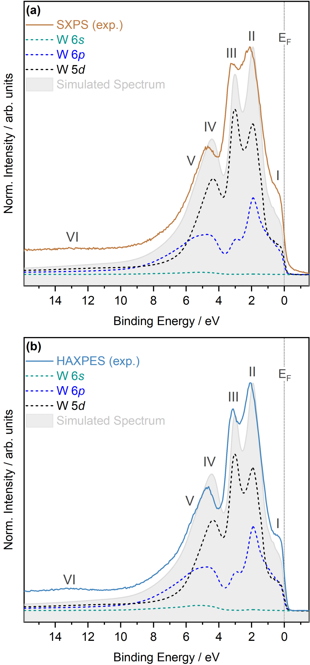
Figure 9: Comparison of the simulated PDOS spectrum calculated using the GW+C approach to the valence band collected with (a) SXPS and (b) HAXPES. The PDOS contributions have been cross section weighted according to the “optimised” method outlined in Section III.3, and as the GW+C approach considers lifetime broadening, no additional broadening was applied. Simulated Spectrum refers to the sum of the weighted PDOS. See the Supplementary Information IX for the GW+C unweighted PDOS.

V Conclusions

This work presents a comprehensive analysis of the relationship between the electronic structure and features in the photoelectron spectrum of tungsten metal, combining state-of-the-art experimental and theoretical approaches.

First, exploration of REELS data enabled the identification of a large number of spectral features related to plasmons and interband transitions. Insights gathered from REELS were used to inform the identification of satellite features in PES core state spectra. In-depth analysis of both SXPS and HAXPES core level spectra provides new insights into the nature of specific transitions underlying the observed satellite features, with spectral functions calculated from GW+C underpinning the experimental assignments. Direct comparisons between the shallow and deep core levels allowed for the identification of hidden, previously not identified satellite features. Cross section effects and the opportunity to access alternative core levels to the commonly used but complex 4f and 4d core levels clearly demonstrate the impact of HAXPES experiments. The deep 3d core level offers a relatively narrow FWHM and small Lorentzian contribution, making it a feasible alternative to the shallow core levels. The core level data are further completed by a detailed investigation of the valence band of tungsten using experiment as well as employing multiple levels of theory. LS-DFT was successfully applied and showed good agreement to conventional cubic-scaling DFT, enabling future studies on large, complex, disordered, multi-metallic systems modelled with LS-DFT with high accuracy and reproducibility.

The present results offer critical insights for both fundamental studies and for crucial scientific and industrial applications involving tungsten, laying the foundation for the exploration of its nanostructures and compounds, as well as device-relevant heterostructures. Finally, the strategy presented here allows future exploration of other transition metals, which have similarly complex photoelectron spectra and electronic structure.

Disclosures

The authors declare no conflicts of interest.

Data Availability

The data that support the findings of this study are available within the article and its supplementary material. Freely accessible versions of all survey, core level and valence band spectra collected with SXPS and HAXPES are available on Figshare at https://doi.org/10.6084/m9.figshare.16432617. All data concerning the BigDFT calculations are openly available in the NOMAD repository at https://dx.doi.org/10.17172/NOMAD/2021.08.27-1. Any further supporting data including the Quantum Espresso DFT and GW+C calculations are available from the corresponding author upon reasonable request.

Supplementary Information

Further details regarding the experimental and computational methods can be found in the Supplementary Information. Additionally, full tabulated data of all values derived from the SXPS and HAXPES core level spectra can also be found in the Supplementary Information. Lastly, a detailed overview of the method and parameters used to construct the simulated core levels and determine the optimum photoionisation cross section weighting, variants of the LS-DFT PDOS calculations using different atom numbers, and survey spectra can also be found in the Supplementary Information.

References

- Smid et al. [1998] I. Smid, M. Akiba, G. Vieider, and L. Plöchl, Journal of Nuclear Materials 258-263, 160 (1998).
- Fujita et al. [2016] H. Fujita, K. Yuyama, X. Li, Y. Hatano, T. Toyama, M. Ohta, K. Ochiai, N. Yoshida, T. Chikada, and Y. Oya, Physica Scripta 2016, 014068 (2016).
- Causey and Venhaus [2001] R. A. Causey and T. J. Venhaus, Physica Scripta 2001, 9 (2001).
- Causey et al. [1999] R. Causey, K. Wilson, T. Venhaus, and W. R. Wampler, Journal of Nuclear Materials 266-269, 467 (1999).
- Abernethy [2017] R. G. Abernethy, Materials Science and Technology 33, 388 (2017).
- Philipps [2011] V. Philipps, Journal of Nuclear Materials 415, S2 (2011).
- Niklasson and Granqvist [2007] G. A. Niklasson and C. G. Granqvist, Journal of Materials Chemistry 17, 127 (2007).
- Walter et al. [2010] M. G. Walter, E. L. Warren, J. R. McKone, S. W. Boettcher, Q. Mi, E. A. Santori, and N. S. Lewis, Chemical Reviews 110, 6446 (2010).
- Migas et al. [2010] D. B. Migas, V. L. Shaposhnikov, and V. E. Borisenko, Journal of Applied Physics 108, 093714 (2010).
- Zheng et al. [2011] H. Zheng, J. Z. Ou, M. S. Strano, R. B. Kaner, A. Mitchell, and K. Kalantar-Zadeh, Advanced Functional Materials 21, 2175 (2011).
- Mardare and Hassel [2019] C. C. Mardare and A. W. Hassel, Physica Status Solidi (A) Applications and Materials Science 216, 1900047 (2019).
- Plappert et al. [2012] M. Plappert, O. Humbel, A. Koprowski, and M. Nowottnick, Microelectronics Reliability 52, 1993 (2012).
- Fugger et al. [2014] M. Fugger, M. Plappert, C. Schäffer, O. Humbel, H. Hutter, H. Danninger, and M. Nowottnick, Microelectronics Reliability 54, 2487 (2014).
- Roshanghias et al. [2014] A. Roshanghias, G. Khatibi, R. Pelzer, and J. Steinbrenner, Surface and Coatings Technology 259, 386 (2014).
- Kleinbichler et al. [2017] A. Kleinbichler, J. Todt, J. Zechner, S. Wöhlert, D. M. Többens, and M. J. Cordill, Surface and Coatings Technology 332, 376 (2017).
- Wach et al. [2020] A. Wach, J. Sá, and J. Szlachetko, Journal of Synchrotron Radiation 27, 689 (2020).
- Manning and Chodorow [1939] M. F. Manning and M. I. Chodorow, Physical Review 56, 787 (1939).
- Mattheiss [1965] L. F. Mattheiss, Physical Review 139, 1893 (1965).
- Loucks [1965] T. L. Loucks, Physical Review 139, 1181 (1965).
- Petroff and Viswanathan [1971] I. Petroff and C. R. Viswanathan, Physical Review B 4, 799 (1971).
- Feder and Sturm [1975] R. Feder and K. Sturm, Physical Review B 12, 537 (1975).
- Posternak and Krakauer [1980] M. Posternak and H. Krakauer, Physical Review B 21, 5601 (1980).
- Mattheiss and Hamann [1984] L. F. Mattheiss and D. R. Hamann, Physical Review B 29, 5372 (1984).
- Jansen and Freeman [1984] H. J. F. Jansen and A. J. Freeman, Physical Review B 30, 561 (1984).
- Wei et al. [1985] S.-H. Wei, H. Krakauer, and M. Weinert, Physical Review B 32, 7792 (1985).
- Legoas et al. [2000] S. B. Legoas, A. A. Araujo, B. Laks, A. B. Klautau, and S. Frota-Pessôa, Physical Review B 61, 10417 (2000).
- Christensen and Feuerbacher [1974] N. E. Christensen and B. Feuerbacher, Physical Review B 10, 2349 (1974).
- Feuerbacher and Christensen [1974] B. Feuerbacher and N. E. Christensen, Physical Review B 10, 2373 (1974).
- Jiang et al. [2010] B. Jiang, F. R. Wan, and W. T. Geng, Physical Review B - Condensed Matter and Materials Physics 81, 134112 (2010).
- Ventelon et al. [2012] L. Ventelon, F. Willaime, C. C. Fu, M. Heran, and I. Ginoux, Journal of Nuclear Materials 425, 16 (2012).
- Sun et al. [2014] S. J. Sun, K. H. Lin, S. P. Ju, and J. Y. Li, Journal of Applied Physics 116, 133704 (2014).
- Fernandez et al. [2015] N. Fernandez, Y. Ferro, and D. Kato, Acta Materialia 94, 307 (2015).
- Zhang et al. [2017] N. Zhang, Y. Zhang, Y. Yang, P. Zhang, Z. Hu, and C. Ge, European Physical Journal B 90 (2017).
- Song et al. [2018] J. Song, Y. C. Zhang, Z. F. Huang, L. Pan, X. Zhang, L. Wang, and J. J. Zou, Journal of Physical Chemistry C 122, 23053 (2018).
- Aryasetiawan et al. [1996] F. Aryasetiawan, L. Hedin, and K. Karlsson, Physical Review Letters 77, 2268 (1996).
- Guzzo et al. [2012] M. Guzzo, J. J. Kas, F. Sottile, M. G. Silly, F. Sirotti, J. J. Rehr, and L. Reining, The European Physical Journal B 85 (2012).
- Lischner et al. [2013] J. Lischner, D. Vigil-Fowler, and S. G. Louie, Physical Review Letters 110 (2013).
- Lischner et al. [2015] J. Lischner, G. K. Pálsson, D. Vigil-Fowler, S. Nemsak, J. Avila, M. C. Asensio, C. S. Fadley, and S. G. Louie, Physical Review B - Condensed Matter and Materials Physics 91 (2015).
- Jiang [2012] H. Jiang, Journal of Physical Chemistry C 116, 7664 (2012).
- Regoutz et al. [2019] A. Regoutz, A. M. Ganose, L. Blumenthal, C. Schlueter, T. L. Lee, G. Kieslich, A. K. Cheetham, G. Kerherve, Y. S. Huang, R. S. Chen, G. Vinai, T. Pincelli, G. Panaccione, K. H. Zhang, R. G. Egdell, J. Lischner, D. O. Scanlon, and D. J. Payne, Physical Review Materials 3 (2019).
- Lu et al. [2021] Q. Lu, H. Martins, J. M. Kahk, G. Rimal, S. Oh, I. Vishik, M. Brahlek, W. C. Chueh, J. Lischner, and S. Nemsak, Communications Physics 4, 143 (2021).
- Hussain et al. [1980] Z. Hussain, C. S. Fadley, S. Kono, and L. F. Wagner, Physical Review B 22, 3750 (1980).
- Jugnet et al. [1987] Y. Jugnet, N. S. Prakash, T. M. Duc, H. C. Poon, G. Grenet, and J. B. Pendry, Surface Science 189, 782 (1987).
- Gaylord and Kevan [1987] R. H. Gaylord and S. D. Kevan, Physical Review B 36, 9337 (1987).
- Gray et al. [2011] A. X. Gray, C. Papp, S. Ueda, B. Balke, Y. Yamashita, L. Plucinski, J. Minár, J. Braun, E. R. Ylvisaker, C. M. Schneider, W. E. Pickett, H. Ebert, K. Kobayashi, and C. S. Fadley, Nature Materials 10, 759 (2011).
- Medjanik et al. [2017] K. Medjanik, O. Fedchenko, S. Chernov, D. Kutnyakhov, M. Ellguth, A. Oelsner, B. Schönhense, T. R. Peixoto, P. Lutz, C. H. Min, F. Reinert, S. Däster, Y. Acremann, J. Viefhaus, W. Wurth, H. J. Elmers, and G. Schönhense, Nature Materials 16, 615 (2017).
- Medjanik et al. [2019] K. Medjanik, S. V. Babenkov, S. Chernov, D. Vasilyev, B. Schönhense, C. Schlueter, A. Gloskovskii, Y. Matveyev, W. Drube, H. J. Elmers, and G. Schönhense, Journal of Synchrotron Radiation 26, 1996 (2019).
- Drube et al. [1986] W. Drube, D. Straub, F. J. Himpsel, P. Soukiassian, C. L. Fu, and A. J. Freeman, Physical Review B 34, 8989 (1986).
- Penchina et al. [1974] C. M. Penchina, E. Sapp, J. Tejeda, and N. Shevchik, Physical Review B 10, 4187 (1974).
- Chen and Roberts [1995] W. Chen and J. T. Roberts, Surface Science 324, 169 (1995).
- Warren et al. [1996] A. Warren, A. Nylund, and I. Olefjord, International Journal of Refractory Metals and Hard Materials 14, 345 (1996).
- Engelhard and Baer [2000] M. Engelhard and D. Baer, Surface Science Spectra 7, 1 (2000).
- Colton and Rabalais [1976] R. J. Colton and J. W. Rabalais, Inorganic Chemistry 15, 236 (1976).
- Egawa et al. [1983] C. Egawa, S. Naito, and K. Tamaru, Surface Science 131, 49 (1983).
- Feuerbacher and Fitton [1973] B. Feuerbacher and B. Fitton, Physical Review Letters 30, 923 (1973).
- Feydt et al. [1998] J. Feydt, A. Elbe, H. Engelhard, G. Meister, C. Jung, and A. Goldmann, Physical Review B 58, 14007 (1998).
- Van Der Veen et al. [1982] J. F. Van Der Veen, F. J. Himpsel, and D. E. Eastman, Physical Review B 25, 7388 (1982).
- Smith et al. [1976] R. J. Smith, J. Anderson, Hermanson J, and Lapeyre G J, Solid State Communications 19, 975 (1976).
- Holmes and Gustafsson [1981] M. I. Holmes and T. Gustafsson, Physical Review Letters 47, 443 (1981).
- Mueller et al. [1988] D. Mueller, A. Shih, E. Roman, T. Madey, R. Kurtz, and R. Stockbauer, Journal of Vacuum Science & Technology A: Vacuum, Surfaces, and Films 6, 1067 (1988).
- Riffe et al. [1990] D. M. Riffe, G. K. Wertheim, P. H. Citrin, and D. N. E. Buchanan, Physica Scripta 41, 1009 (1990).
- Mullins and Lyman [1993] D. R. Mullins and P. F. Lyman, Surface Science 285, 473 (1993).
- Ley et al. [1975] L. Ley, F. R. Mcfeely, S. P. Kowalczyk, J. G. Jenkin, and D. A. Shirley, Physical Review B 11, 600 (1975).
- Steiner et al. [1978] P. Steiner, H. Höchst, and S. Hüfner, Zeitschrift für Physik B Condensed Matter 30, 129 (1978).
- Th et al. [1979] P. M. Th, V. Attekum, and J. M. Trooster, Physical Review B 20, 2335 (1979).
- Bates Jr et al. [1979] C. W. Bates Jr, G. K. Wertheim, and D. N. E. Buchanan, Physics Letters 72, 178 (1979).
- Kurth et al. [2003] M. Kurth, P. C. Graat, and E. J. Mittemeijer, Applied Surface Science 220, 60 (2003).
- Leiro et al. [1983] J. Leiro, E. Minni, and E. Suoninen, Journal of Physics F: Metal Physics 13, 215 (1983).
- Weaver et al. [1975] J. H. Weaver, C. G. Olson, and D. W. Lynch, Physical Review B 12, 1293 (1975).
- Luscher [1977] P. E. Luscher, Surface Science 66, 167 (1977).
- Kalha et al. [2021a] C. Kalha, S. Bichelmaier, N. K. Fernando, J. V. Berens, P. K. Thakur, T.-L. Lee, J. J. Gutiérrez-Moreno, S. Mohr, L. E. Ratcliff, M. Reisinger, J. Zechner, M. Nelhiebel, and A. Regoutz, Journal of Applied Physics 129, 195302 (2021a).
- Hohenberg and Kohn [1964] P. Hohenberg and W. Kohn, Physical Review 136, 864 (1964).
- Kohn and Sham [1965] W. Kohn and L. J. Sham, Physical Review 140, 1133 (1965).
- Hybertsen and Louie [1986] M. S. Hybertsen and S. G. Louie, Physical Review B 34, 5390 (1986).
- Guzzo et al. [2011] M. Guzzo, G. Lani, F. Sottile, P. Romaniello, M. Gatti, J. J. Kas, J. J. Rehr, M. G. Silly, F. Sirotti, and L. Reining, Physical Review Letters 107 (2011).
- Caruso et al. [2015] F. Caruso, H. Lambert, and F. Giustino, Physical Review Letters 114 (2015).
- Mohr et al. [2014] S. Mohr, L. E. Ratcliff, P. Boulanger, L. Genovese, D. Caliste, T. Deutsch, and S. Goedecker, The Journal of Chemical Physics 140, 204110 (2014).
- Mohr et al. [2015] S. Mohr, L. E. Ratcliff, L. Genovese, D. Caliste, P. Boulanger, S. Goedecker, and T. Deutsch, Physical Chemistry Chemical Physics 17, 31360 (2015).
- Lee and Duncan [2018] T. L. Lee and D. A. Duncan, Synchrotron Radiation News 31, 16 (2018).
- Tanuma et al. [1993] S. Tanuma, C. J. Powell, and D. R. Penn, Surface and Interfacec Analysis 21, 165 (1993).
- Giannozzi et al. [2009] P. Giannozzi, S. Baroni, N. Bonini, M. Calandra, R. Car, C. Cavazzoni, D. Ceresoli, G. L. Chiarotti, M. Cococcioni, I. Dabo, A. Dal Corso, S. De Gironcoli, S. Fabris, G. Fratesi, R. Gebauer, U. Gerstmann, C. Gougoussis, A. Kokalj, M. Lazzeri, L. Martin-Samos, N. Marzari, F. Mauri, R. Mazzarello, S. Paolini, A. Pasquarello, L. Paulatto, C. Sbraccia, S. Scandolo, G. Sclauzero, A. P. Seitsonen, A. Smogunov, P. Umari, and R. M. Wentzcovitch, Journal of Physics Condensed Matter 21, 395502 (2009).
- Ratcliff et al. [2020] L. E. Ratcliff, W. Dawson, G. Fisicaro, D. Caliste, S. Mohr, A. Degomme, B. Videau, V. Cristiglio, M. Stella, M. D’Alessandro, S. Goedecker, T. Nakajima, T. Deutsch, and L. Genovese, The Journal of Chemical Physics 152, 194110 (2020).
- Perdew et al. [1996] J. P. Perdew, K. Burke, and M. Ernzerhof, Physical Review Letters 77, 3865 (1996).
- Löwdin [1950] P. Löwdin, Journal of Chemical Physics 18, 365 (1950).
- Löwdin [1970] P.-O. Löwdin, in Advances in Quantum Chemistry, Vol. 5 (Academic Press, 1970) pp. 185–199.
- Mulliken [1955] R. S. Mulliken, The Journal of Chemical Physics 23, 1833 (1955).
- Mohr et al. [2017] S. Mohr, M. Masella, L. E. Ratcliff, and L. Genovese, Journal of Chemical Theory and Computation 13, 4079 (2017).
- Dawson et al. [2020] W. Dawson, S. Mohr, L. E. Ratcliff, T. Nakajima, and L. Genovese, Journal of Chemical Theory and Computation 16, 2952 (2020).
- Deslippe et al. [2012] J. Deslippe, G. Samsonidze, D. A. Strubbe, M. Jain, M. L. Cohen, and S. G. Louie, Computer Physics Communications 183, 1269 (2012).
- Deslippe et al. [2013] J. Deslippe, G. Samsonidze, M. Jain, M. L. Cohen, and S. G. Louie, Physical Review B - Condensed Matter and Materials Physics 87, 165124 (2013).
- Scofield [1973] J. H. Scofield, Theoretical Photoionization Cross Sections from 1 to 1500 keV, Tech. Rep. (Lawrence Livermore Laboratory, 1973).
- Mudd et al. [2014] J. J. Mudd, T. L. Lee, V. Muñoz-Sanjosé, J. Zúñiga-Pérez, D. J. Payne, R. G. Egdell, and C. F. McConville, Physical Review B - Condensed Matter and Materials Physics 89, 165305 (2014).
- Kalha et al. [2020] C. Kalha, N. Fernando, and A. Regoutz, “Digitisation of Scofield Photoionisation Cross Section Tabulated Data,” (2020).
- Panaccione et al. [2005] G. Panaccione, G. Cautero, M. Cautero, A. Fondacaro, M. Grioni, P. Lacovig, G. Monaco, F. Offi, G. Paolicelli, M. Sacchi, N. Stojić, G. Stefani, R. Tommasini, and P. Torelli, Journal of Physics Condensed Matter 17, 2671 (2005).
- J Jackson et al. [2018] A. J Jackson, A. M Ganose, A. Regoutz, R. G. Egdell, and D. O Scanlon, Journal of Open Source Software 3, 773 (2018).
- Harrower [1956] G. A. Harrower, Physical Review 102, 340 (1956).
- Tharp and Scheibner [1967] L. N. Tharp and E. J. Scheibner, Journal of Applied Physics 38, 3320 (1967).
- Porteus and Faith [1970] J. O. Porteus and W. N. Faith, Physical Review B 2, 1532 (1970).
- Edwards and Propst [1971] D. Edwards and F. M. Propst, The Journal of Chemical Physics 55, 5175 (1971).
- Burkstrand et al. [1972] J. M. Burkstrand, T. L. Propst, T. L. Cooper, and D. E. Edwards, Surface Science 29, 663 (1972).
- Stein and Stern [1972] R. J. Stein and R. M. Stern, Journal of Vacuum Science and Technology 9, 743 (1972).
- Avery [1981] N. R. Avery, Surface Science 111, 358 (1981).
- Gergely [1981] G. Gergely, Surface and Interface Analysis 3, 201 (1981).
- Shinar et al. [1984] R. Shinar, T. Maniv, and M. Folman, Surface Science 141, 158 (1984).
- Cżyzewski and Krajniak [1990] J. J. Cżyzewski and J. Krajniak, Surface Science 231, 18 (1990).
- Cżyzewski et al. [1991] J. J. Cżyzewski, J. Krajniak, and S. Klein, Surface Science 247, 389 (1991).
- Ritchie [1957] R. H. Ritchie, Physical Review 106, 874 (1957).
- Oura et al. [2003] K. Oura, M. Katayama, A. V. Zotov, V. G. Lifshits, and A. A. Saranin, Surface Science: An Introduction, Advanced Texts in Physics (Springer Berlin Heidelberg, 2003).
- Weaver et al. [1973] J. H. Weaver, D. W. Lynch, and C. G. Olson, Physical Review B 7, 4311 (1973).
- Weaver et al. [1974] J. H. Weaver, D. W. Lynch, and C. G. Olson, Physical Review B 10, 501 (1974).
- Romaniello et al. [2006] P. Romaniello, P. L. De Boeij, F. Carbone, and D. Van Der Marel, Physical Review B - Condensed Matter and Materials Physics 73, 075115 (2006).
- Ballu et al. [1976] Y. Ballu, J. Lecante, and D. M. Newns, Physical Letters 57, 159 (1976).
- Powell et al. [1958] C. J. Powell, J. L. Robins, and J. B. Swan, Physical Review 110, 657 (1958).
- Scheibner and Tharp [1967] E. J. Scheibner and L. N. Tharp, Surface Science 8, 247 (1967).
- Doniach and Šunjić [1969] S. Doniach and M. Šunjić, Journal of Physics C Solid State Physics 3, 285 (1969).
- Hüfner et al. [1975] S. Hüfner, G. K. Wertheim, and J. H. Wernick, Solid State Communications 17, 417 (1975).
- Wertheim and Walker [1976] G. K. Wertheim and L. R. Walker, Journal of Physics F: Metal Physics 6, 2297 (1976).
- Biloen and Pott [1973] P. Biloen and G. T. Pott, Journal of Catalysis 30, 169 (1973).
- McGuire et al. [1973] G. E. McGuire, G. K. Schweitzer, and T. A. Carlson, Inorganic Chemistry 12, 2450 (1973).
- Ng and Hercules [1976] K. T. Ng and D. M. Hercules, Journal of Physical Chemistry 80, 2094 (1976).
- Colton et al. [1978] R. J. Colton, A. M. Guzman, and J. W. Rabalais, Journal of Applied Physics 49, 409 (1978).
- Nyholm et al. [1980] R. Nyholm, A. Berndtsson, and N. Mahrtensson, Journal of Physics C Solid State 13, 1091 (1980).
- Takano and Isobe [1989] I. Takano and S. Isobe, Applied Surface Science 37, 25 (1989).
- Powell [2012] C. J. Powell, Journal of Electron Spectroscopy and Related Phenomena 185, 1 (2012).
- Sundberg et al. [2014] J. Sundberg, R. Lindblad, M. Gorgoi, H. Rensmo, U. Jansson, and A. Lindblad, Applied Surface Science 305, 203 (2014).
- Perkins et al. [1991] S. T. Perkins, D. E. Cuuen, M. H. Chen, and J. H. Hubbell, Tables and Graphs of Atomic Subshell and Relaxation Data Derived from the LLNL Evaluated Atomic Data Library (EADL), Z = 1-100, Tech. Rep. (Lawrence Livermore National Laboratory, 1991).
- Campbell and Papp [2001] J. L. Campbell and T. Papp, Atomic Data and Nuclear Data Tables 77, 1 (2001).
- Fuggle and Alvarado [1980] J. C. Fuggle and S. F. Alvarado, Physical Review A 22, 1615 (1980).
- Ohno and Van Riessen [2003] M. Ohno and G. A. Van Riessen, Journal of Electron Spectroscopy and Related Phenomena 128, 1 (2003).
- Panaccione and Kobayashi [2012] G. Panaccione and K. Kobayashi, Surface Science 606, 125 (2012).
- Church et al. [2015] J. R. Church, C. Weiland, and R. L. Opila, Applied Physics Letters 106, 171601 (2015).
- Regoutz et al. [2018] A. Regoutz, M. Mascheck, T. Wiell, S. K. Eriksson, C. Liljenberg, K. Tetzner, B. A. Williamson, D. O. Scanlon, and P. Palmgren, Review of Scientific Instruments 89 (2018).
- Kalha et al. [2021b] C. Kalha, N. K. Fernando, P. Bhatt, F. O. L. Johansson, A. Lindblad, H. Rensmo, L. Z. Medina, R. Lindblad, S. Siol, L. P. H. Jeurgens, C. Cancellieri, K. Rossnagel, K. Medjanik, G. Schönhense, M. Simon, A. X. Gray, S. Nemšák, P. Lömker, C. Schlueter, and A. Regoutz, Journal of Physics: Condensed Matter 33, 233001 (2021b).
- Wagner [1978] C. D. Wagner, Journal of Vacuum Science & Technology 15, 518 (1978).
- Inglesfield [1981] J. E. Inglesfield, Solid State Communications 40, 467 (1981).
- Woicik et al. [2015] J. C. Woicik, C. Weiland, and A. K. Rumaiz, Physical Review B - Condensed Matter and Materials Physics 91, 201412 (2015).
- Fleisch and Mains [1982] T. H. Fleisch and G. J. Mains, The Journal of Chemical Physics 76, 780 (1982).
- Werfel and Minni [1983] F. Werfel and E. Minni, Journal of Physics C Solid State Physics 16, 6091 (1983).
- Buabthong et al. [2017] P. Buabthong, N. Becerra Stasiewicz, S. Mitrovic, and N. S. Lewis, Surface Science Spectra 24, 024001 (2017).
- Ławniczak-Jabłońska and Heinonen [1988] K. Ławniczak-Jabłońska and M. Heinonen, Journal of Physics F: Metal Physics 18, 2451 (1988).
- Northrup et al. [1989] J. E. Northrup, M. S. Hybertsen, and S. G. Louie, Physical Review B 39, 8198 (1989).
- Qiu et al. [2020] D. Y. Qiu, S. Coh, M. L. Cohen, and S. G. Louie, Physical Review B 101 (2020).
- Strocov et al. [1998] V. N. Strocov, R. Claessen, G. Nicolay, S. Hüfner, A. Kimura, A. Harasawa, S. Shin, A. Kakizaki, P. O. Nilsson, H. I. Starnberg, and P. Blaha, Physical Review Letters 81, 4943 (1998).
- Marini et al. [2002] A. Marini, G. Onida, and R. Del Sole, Physical Review Letters 88, 4 (2002).