[1em]1em1em\thefootnotemark
Reshetikhin–Turaev TQFTs
close under generalised orbifolds
Abstract
We specialise the construction of orbifold graph TQFTs introduced in [3] to Reshetikhin–Turaev defect TQFTs. We explain that the modular fusion category constructed in [18] from an orbifold datum in a given modular fusion category is a special case of the Wilson line ribbon categories introduced as part of the general theory of orbifold graph TQFTs. Using this, we prove that the Reshetikhin–Turaev TQFT obtained from is equivalent to the orbifold of the TQFT for with respect to the orbifold datum .
1 Introduction and summary
The generalised orbifold construction is a procedure to obtain a new TQFT from a given defect TQFT, that is, a TQFT defined on stratified bordisms [6]. The procedure is best understood as an internal state sum construction and indeed, the Turaev–Viro–Barrett–Westbury state sum TQFT is in this sense a generalised orbifold of the trivial TQFT [8].
In [3] we extended the generalised orbifold construction to 3-dimensional graph TQFTs. By a graph TQFT we mean a TQFT defined on oriented bordisms with embedded ribbon graphs coloured by objects and morphisms in a given ribbon category. The strands and coupons of these ribbon graphs can be interpreted as Wilson lines and junction points.
The starting point for the generalised orbifold construction are 3-dimensional defect TQFTs as introduced in [4, 6]. Such TQFTs are symmetric monoidal functors whose source categories have stratified 3-dimensional bordisms as morphisms, with all strata carrying labels taken from a prescribed set of “defect data” . In particular, 1- and 2-strata are interpreted as line and surface defects, respectively.
The generalised orbifold construction takes a defect TQFT
| (1.1) |
and a particular set of defect labels as input to produce a graph TQFT
| (1.2) |
As explained in [3] and reviewed in Section 3.3 below, this is done by decomposing bordisms into special stratifications that we call “admissible skeleta”, decorating them with the chosen orbifold datum , and then evaluating with to obtain as a colimit. The defining conditions on are such that this construction is independent of the choice of skeleta. Embedded ribbon graphs are treated by projecting them on the 1- and 2-strata of the chosen skeleta. Compatibility constraints naturally lead to the ribbon category of Wilson lines , which is used to colour ribbon graphs of the orbifold theory.
In this paper we will apply the construction in [3] to Reshetikhin–Turaev theories. Given a modular fusion category , the Reshetikhin–Turaev construction [20] provides a 3-dimensional graph TQFT
| (1.3) |
where the source category is given by (a central extension of) 3-dimensional bordisms with embedded -coloured ribbon graphs, cf. Section 3.1 below. Every Reshetikhin–Turaev graph TQFT can be lifted to a defect TQFT
| (1.4) |
with both line defects and surface defects. Indeed, as explained in [17, 13, 7], an internal 2-dimensional state sum construction identifies -separable symmetric Frobenius algebra in as labels for surface defects, and certain modules over such algebras as labels for line defects, see Section 3.2 for more details. The graph TQFT can be viewed as the restriction of to bordisms without surface defects.
Our main result is to show that the general construction of orbifold graph TQFTs (1.2), applied to the defect TQFT in (1.4), produces a graph TQFT which is again of Reshetikhin–Turaev type. To state the precise result, we use that an orbifold datum111What we call an “orbifold datum” here is called a “special orbifold datum” in [8, 3]. Since in this paper only special orbifold data appear, we will drop the “special”. for can be described as a collection of algebraic data in the underlying modular fusion category (see Section 2.3). The resulting ribbon category was first studied in [18], where it was shown to be a modular fusion category, provided that is simple. A simple orbifold datum for therefore yields two – a priori distinct – graph TQFTs: obtained from the Reshetikhin–Turaev construction based on , and
| (1.5) |
obtained as the -orbifold of . We show in Theorem 4.1 that they are the same:
Theorem. Let be a simple orbifold datum in a modular fusion category . Then the graph TQFTs and are isomorphic.
The proof is inspired by a similar equivalence between the graph TQFTs of Turaev–Viro–Barrett–Westbury type obtained from a spherical fusion category , and of Reshetikhin–Turaev type obtained from the Drinfeld centre . In fact, this result is a special case of our Theorem 4.1 as there is an orbifold datum in the category of finite-dimensional vector spaces such that is isomorphic to the Turaev–Viro–Barrett–Westbury TQFT based on [8, Sect. 4], while the associated modular fusion category is equivalent to [18, Sect. 4.2].
More specifically, we proceed analogously to [21, Ch. 17]. The key technical lemma (cf. Lemma 4.2) is that the following three conditions on monoidal functors with values in vect imply a unique monoidal equivalence : (i) is non-degenerate, (ii) for all objects in the source category, and (iii) and agree on all endomorphisms of the unit object. Applied to our case of and , we observe that (i) all Reshetikhin–Turaev TQFTs are known to be non-degenerate [20, Ch. IV], (ii) one can define surjective linear maps from the state spaces of to those of (Section 4.3), and (iii) the invariants associated to closed manifolds with embedded ribbon graphs agree (Section 4.2). Apart from rather explicit computations in modular fusion categories, the main technical work in our proof is to obtain “skeleta from surgery” (Section 4.1), mediating between the surgery construction in Reshetikhin–Turaev theory and the decompositions needed for the orbifold construction.
There are a number of natural questions which arise from the above theorem. For example, given two modular fusion categories and , one can ask whether is isomorphic to a generalised orbifold of . It will be shown in [19] that this happens if and only if and are Witt equivalent [10]. In fact Witt equivalence is also the obstruction which determines if two TQFTs of Reshetikhin–Turaev type can be joined by a surface defect in the first place [13, 16].
Another direction to continue this work is to not only consider line defects in the orbifold theory, but also surface defects, and, in fact, more generally surface defects between different orbifolds. This amounts to a 3-dimensional version of the orbifold completion introduced in two dimensions in [5]. The expected result is that Reshetikhin–Turaev TQFTs for a given Witt class (with defects of all dimensions, and with 3-strata labelled by possibly different modular fusion categories in the given Witt class) are already orbifold complete. Ideas related to orbifold completion have also been pursued in the context of framed (as opposed to oriented) tangential structures and higher idempotent completions in [14].
Acknowledgements
N. C. is supported by the DFG Heisenberg Programme. V. M. is partially supported by the DFG Research Training Group 1670. I. R. is partially supported by the Cluster of Excellence EXC 2121 “Quantum Universe” - 390833306.
2 Background
We review some prerequisites on modular fusion categories (Section 2.1), algebras and modules (Section 2.2), and orbifold constructions (Section 2.3) which will be used extensively in the later sections.
2.1 Modular fusion categories
A modular fusion category over an algebraically closed field is a braided spherical fusion category over whose braiding is non-degenerate. Recall, e. g. from [20, 11], that this means in particular that is a semisimple -linear monoidal category with only finitely many isomorphism classes of simple objects, and with simple tensor unit. Moreover, invoking the spherical structure, every object has a simultaneous left- and right- dual with the (co)evaluation maps denoted by
| (2.1) | |||
| (2.2) |
satisfying the pivotality conditions, see e. g. [5, Lem. 2.12]. Our convention is to read string diagrams from bottom to top and from right to left, such that the braiding morphisms as well as their inverses are depicted as follows:
| (2.3) |
Non-degeneracy of the braiding means that if for all , then is isomorphic to for some .
The above structure maps are subject to the standard coherence constraints (see e. g. [11, Sect. 2.10 & 4.7 & 8.1]), and to the sphericality condition which states that for every endomorphism , the left and right traces agree:
| (2.4) |
The quantum dimension of an object is
| (2.5) |
and the global dimension of is
| (2.6) |
where here and below by we denote a set of representatives of isomorphism classes of simple objects in such that . For a modular fusion category one has (see [20, Sect. II.3.2]). The construction of the TQFT in Section 3 requires the choice of a square root of the global dimension,
| (2.7) |
An important invariant of a modular fusion category is its “anomaly”. To give the definition, we recall the twist automorphisms
| (2.8) |
and set222Note that we slightly abuse notation by identifying for simple objects ; similarly we often view traces and quantum dimensions as scalars.
| (2.9) |
Then the anomaly of the pair is the scalar
| (2.10) |
That the two ratios are indeed equal is shown in [2, Cor. 3.1.11]. For , is a phase, which is why one considers the ratios in (2.10) rather than just .
2.2 Algebras and modules
A -separable symmetric Frobenius algebra is an object with the structure of an associative unital algebra and a coassociative counital coalgebra, such that, with denoting the (co)multiplication and (co)unit, we have
| (2.11) |
A (left) module of a Frobenius algebra is automatically a (left) comodule with the coaction
| (2.12) |
If is a -separable symmetric Frobenius algebra, the tensor product over of a right module and a left module can be realised as the image of a projector, namely
| (2.13) |
where in the last equality the expression (2.12) was used.333 Since is symmetric one does not need to distinguish between action and coaction, and hence we will not do so in our graphical notation. The relative tensor product equips the category of --bimodules with a monoidal structure.
If is any algebra, then we endow with an algebra structure with multiplication and unit
| and | (2.14) |
respectively. Then a right -module is equivalently an object with two -actions such that
| (2.15) |
where we used indices to distinguish between the two actions. For a left -module , we denote by and the relative tensor products with respect to the corresponding -actions.
2.3 Orbifold data and associated modular fusion categories
We review the notion of an orbifold datum in a modular fusion category as introduced in [8, Sect. 3.2].444Recall from footnote 1 that we always implicitly assume an orbifold datum to be special. It is a tuple
| (2.16) |
that consists of
-
•
a -separable symmetric Frobenius algebra in ,
-
•
an --bimodule ,
-
•
--bimodule maps and ,
-
•
an invertible --bimodule map ,
-
•
an invertible scalar
subject to the conditions (O1)–(O8) which we list in Figure A.1 in Appendix A. Here and below we use the following abbreviations for the endomorphisms obtained from via different -actions on and on an arbitrary --bimodule :
| (2.17) |
We also abbreviate and write an index next to the morphisms , , to distinguish between different bimodules if needed. Note that if , then .
In keeping with the notation , in (2.15), given a right -module it is convenient to write for .
Definition 2.1.
Given an orbifold datum in , as in [18, Sect. 3] we define the category to have
- •
-
•
morphisms: is an --bimodule morphism such that
(2.18)
Let us state some properties of the category . We refer to [18] for more details and the proofs.
-
1.
is a multifusion category with the tensor product
(2.19) where the -crossings are
(2.20) and unit is taken to be , where
(2.21) An orbifold datum is called simple if is fusion, i. e. .
-
2.
is spherical where the dual of an object is defined to have as the underlying --bimodule and the crossing morphisms are induced from those of . The adjunction maps are:
(2.22) (2.23) If is a simple orbifold datum one can compute the trace of a morphism as follows:
(2.24) with holding automatically. On the right-hand side of (2.24), is treated as a morphism in .
-
3.
is braided with the braiding morphisms of given by
(2.25) If is a simple orbifold datum, one has ([18, Thm. 3.17]):
Theorem 2.2.
For a simple orbifold datum in , is a modular fusion category with
(2.26) -
4.
Given two objects and any morphism between the underlying objects in , the averaged morphism defined by
(2.29) is a bimodule morphism and satisfies (2.18), i. e. it is a morphism in . In fact, the mapping acts as an idempotent projecting onto seen as a subspace of .
-
5.
A useful tool to work with the category is the pipe functor
(2.30) from [18, Sect. 3.3]. It is biadjoint to the forgetful functor and can be seen as the free construction of an object of . For a bimodule and a bimodule morphism , the underlying --bimodule over the object as well the morphism are defined respectively by
(2.31) where the horizontal lines in the definition of denote the inclusion into and projection onto the image defining and .
Remark 2.3.
The definition (2.31) of the pipe functor has a more intuitive interpretation in terms of the Reshetikhin–Turaev defect TQFT as depicted in Figure 6(a) below. We review this in more detail later in Section 3.2. More generally, pipe functors can be analogously defined for arbitrary 3-dimensional defect TQFTs and the corresponding notion of an orbifold datum in it. We do this in Appendix B.
3 Reshetikhin–Turaev theory
We review the definitions and some properties of three variants of Reshetikhin–Turaev type TQFTs: the graph TQFT (Section 3.1), the defect TQFT (Section 3.2), and the orbifold graph TQFT (Section 3.3). The latter is an explicit example of the orbifold graph TQFTs introduced in [3].
3.1 Reshetikhin–Turaev graph TQFT
We fix a modular fusion category . The Reshetikhin–Turaev graph TQFT is a symmetric monoidal functor
| (3.1) |
and we give a brief description of the source category and of the construction of below. A detailed description can be found in [20, Ch. IV].
Bordisms with ribbon graphs
We use the terminology and conventions of [3, Sect. 2.3 & 3.2] (adapted from [21]) in which the category is said to have -coloured punctured surfaces as objects and -coloured ribbon bordisms as morphisms. A -coloured ribbon bordism is a pair consisting of an oriented -dimensional bordism and an embedded -coloured ribbon graph . A -coloured punctured surface is an oriented -dimension manifold with a finite set of distinguished points called punctures (or marked points). The punctures serve as possible endpoints of strands of embedded ribbon graphs and are labelled by triples , where would label the adjacent strand, is a tangent vector to account for its framing, and is a sign indicating its direction.
The Reshetikhin–Turaev TQFT acts on an extension of the category , which is defined as follows. Objects of are pairs , where is a -coloured punctured surface and is a Lagrangian subspace. A morphism in is a pair , where is a morphism in , and . The unit of an object is the cylinder . The Lagrangian subspaces are only needed for composition: for and , their composition in is given by
| (3.2) |
where denotes the Maslov index of the corresponding Lagrangian subspaces associated to , while and denote the Lagrangian actions induced by and on and , respectively, see [20, Sect. IV.3 & IV.4]. The monoidal product of is given by disjoint union, where for bordisms the integers are added. The symmetric structure of is analogous to that of .
Invariants of closed manifolds
Since is a ribbon category, one has a functor , where is the category of -coloured ribbon graphs. In particular, for every closed -coloured ribbon graph one obtains a scalar invariant .
Recall, e. g. from [20, Sect. II.2.1], that all compact connected closed oriented -manifolds can be obtained by performing surgery along an (uncoloured and undirected) ribbon link in . The procedure is the following: Given a ribbon link , let be a tubular neighbourhood of with disjoint components , such that lies in the centre of . Let be a curve on the boundary of the closure of induced by the framing of the component and let
| (3.3) |
be a diffeomorphism, such that . The manifold
| (3.4) |
is then said to be obtained by surgery on along . In other words, is obtained from by cutting out solid tori and glueing them back via diffeomorphisms of their boundaries. We note that it is possible for different links to yield the same manifold, e. g. can be obtained both from the empty link or from the link with one component which has a single twist. In general, two links yield the same 3-manifold iff they are related by a finite sequence of the so-called Kirby moves, see e. g. [20, Sect. II.3.1].
If is presented by surgery along a framed link , we obtain a -coloured ribbon graph in by labelling each component of with the object
| (3.5) |
and adding a single vertex labelled by the morphism
| (3.6) |
on each component circle. From one then obtains the invariant (see [20, Thm. II.2.2.2])
| (3.7) |
where is the signature of the linking number matrix of , is the number of components of , and the scalars and are as in (2.7) and (2.10), respectively.
The invariant is readily lifted to extended -coloured ribbon bordisms of the form . Indeed, if comes with an embedded -coloured ribbon graph , then the same formula as in (3.7) applies except for an additional anomaly factor , and the evaluation functor is instead applied to the -coloured ribbon graph obtained by combining and , which by abuse of notation we denote (even though and may be non-trivially entangled):
| (3.8) |
see [20, Thm. II.2.3.2] and [20, Sect. IV.9.2] for more details.
Graph TQFT
We are now ready to define the Reshetikhin–Turaev graph TQFT .
For a given object , let (respectively ) be the -vector space freely generated by extended -coloured ribbon bordisms of the form (respectively ). In terms of the pairing
| (3.9) |
one defines the state space associated to to be
| (3.10) |
where is the right radical of the pairing , consisting of those elements with for all .
For a morphism in , the action of is defined as
| (3.11) |
Remark 3.1.
-
(i)
The definition above uses the universal construction of [1]. It does not in general guarantee that the functor obtained this way has a symmetric monoidal structure, but this was proven in [9] for a generalisation of the Reshetikhin–Turaev TQFT obtained from a not necessarily semisimple modular tensor category. This generalisation yields the above construction in the semisimple case. The proof of monoidality fails if the objects of are not equipped with Lagrangian subspaces, so the use of the extended category is necessary (see [15] for more details on this).
-
(ii)
The original definition of the Reshetikhin–Turaev TQFT in [20, Ch. IV] gives a symmetric monoidal functor , but it does not use the universal construction, so a priori it is not clear that the TQFT of [20] and as defined above are isomorphic. However this follows from Lemma 4.2 below, as the two TQFTs give the same invariants on closed manifolds (cf. [20, Thm. II.2.3.2]) and have isomorphic state spaces (compare [20, (IV. 1.4.a)] and [9, Prop. 4.16]).
Next we summarise some properties of that will be needed below.
Property 3.2.
From the definition it follows that the graph TQFT is linear with respect to addition and scalar multiplication of coupons of embedded ribbon graphs. Moreover, upon evaluation one can compose the coupons as well as remove a coupon labelled with an identity morphism, i. e. the following exchanges are allowed:
| (3.12) |
By the terminology of [21, Sect. 15.2.3], graph TQFTs with this property are called regular. In addition, one can replace crossings etc. by the corresponding morphisms, in other words, one can perform graphical calculus on the embedded ribbon graphs. For example, if some part of a ribbon graph in a -bordism is contained in the interior of an embedded closed 3-ball, then it can be exchanged for a single coupon labelled with without changing the value of .
Property 3.3.
Let be a -sphere with negatively oriented punctures labelled by objects and positively oriented punctures labelled by . One has the following isomorphism of vector spaces:
| (3.13) |
is a solid ball with an -labelled coupon. This follows from the description of the TQFT via the universal construction, see Remark 3.1. In general, the state space of any punctured surface is spanned by solid handlebodies with embedded ribbon graphs.
Property 3.4.
The invariants of some simple examples of closed -manifolds are:
| (3.14) | |||
| (3.15) |
The -invariant allows one to rewrite the formula (3.8) for the invariant of a ribbon -manifold represented by the surgery link in as
| (3.16) |
The other two invariants are simply instances of a more general observation: Due to the monoidal functoriality of (or in fact any graph TQFT), for any surface the invariant of is the trace of the identity map on . If , it is equal to the dimension of the state space of , otherwise to the dimension modulo , i. e.
| (3.17) |
We have already seen explicitly in (3.13) that , and the state space of a punctureless torus has a basis consisting of solid tori with non-contractible loops labelled by .
3.2 Reshetikhin–Turaev TQFT with line and surface defects
In this section we outline the construction of a defect TQFT
| (3.18) |
which lifts the Reshetikhin–Turaev TQFT reviewed in Section 3.1 to decorated bordisms with embedded ribbons as well as embedded surfaces. The details of the definition of are the main content of [7].
Defect bordisms for Reshetikhin–Turaev TQFT
Let us briefly describe the source category of the defect TQFT .
For details on defect bordisms and TQFTs we refer to [4, 6] and the summary in [3, Sect. 3]. Here we just mention that the objects and morphisms of the category of defect surfaces and defect bordisms are stratified surfaces and -dimensional bordisms, whose strata are oriented and carry labels from a so-called set of defect data . The latter consists of sets where elements of are used to label the -dimensional strata of defect bordisms, as well as information about which labels can be assigned to adjacent strata. For every defect TQFT there is the so-called -completion, where one expands the set by labelling the -strata with elements of state spaces of small stratified -spheres surrounding them, see [6, Sect. 2.4].
For a modular fusion category , there is a set of defect data with
-
•
: -strata have no labels, or equivalently they all carry the same label .
-
•
: -strata are labelled by -separable symmetric Frobenius algebras in .
-
•
: all -strata are assigned a framing. A -stratum that has no adjacent -strata is labelled by an object of .
Suppose a -stratum has adjacent -strata. Let the labels of them be -separable symmetric Frobenius algebras . We then label with an ---multimodule , i. e. a module over , or equivalently a module over all the algebras simultaneously such that for the - and -actions commute with respect to the braiding (as in (2.15) for , ). The framing of an -labelled -stratum will be taken to be the vector field normal to the adjacent -stratum with the label .
-
•
: -strata are added by the usual completion procedure mentioned above.
Remark 3.5.
-
(i)
In [7] a slightly different set of labels for -strata is used. In particular, the multimodules are equipped with a so-called cyclic structure, the purpose of which is to eliminate the need for -strata to have framings.
- (ii)
-
(iii)
It is possible to further generalise the defect TQFT so that the 3-strata can be labelled by different modular fusion categories, see [16].
The extension relates to in the same way as relates to , i. e. the objects (defect surfaces) are paired with Lagrangian subspaces, and the morphisms (defect bordisms) are paired with integers so that the composition is as in (3.2). For convenience we will often suppress these extra data of the extension below, as they only interact trivially with our arguments.
Ribbonisation
We will define the Reshetikhin–Turaev defect TQFT in terms of the “ribbonisation” map
| (3.19) |
which, as will momentarily become apparent, is not a functor since it does not preserve identity morphisms and depends on auxiliary data.
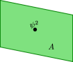
We use the terminology of [3] where a skeleton (here also -skeleton) of an oriented -manifold is a stratification, dividing into a finite collection of open discs and (in case has boundary) half-discs, and each -stratum has exactly three adjacent -strata. A skeleton is then called admissible if its - and -strata are oriented by a local order on the -strata, meaning that the -strata adjacent to a -stratum cannot all be directed towards or away from it. A choice of a skeleton on induces a stratification on the boundary , consisting of a finite set of oriented points dividing it into a collection of open intervals; we will call such a stratification a -skeleton of . Any -skeleton on can be extended to a -skeleton on .
Let be a defect surface. Pick a set of -skeleta for the -strata of . We define
| (3.20) |
to be the underlying oriented surface with the set of punctures , where is the set of -strata of and runs over the -strata of , and is the set of vertices in the chosen 0-skeleton of . For a -stratum labelled with , each point is made into a puncture by decorating it with triple , where is a tangent vector normal to the orientation of , and is the orientation of .
For a defect bordism , let be a set of -skeleta for the -strata of which restricts to sets of -skeleta for the -strata of . We define
| (3.21) |
to be the underlying -manifold with an embedded ribbon graph obtained as follows: the strands are the (already framed, oriented and labelled) -strata of and the -strata of the skeleta for each -stratum , framed by tangent vectors normal to and labelled by the same algebra object as . The -strata of are then replaced by coupons labelled with the (co)multiplication of , while the intersection points of with a -stratum of are labelled by the appropriate (co)action of on the multimodule labelling .
Reshetikhin–Turaev defect TQFT
Let be an object in , and let be two sets of 0-skeleta for its 1-strata. Consider the defect cylinder . For any choice of a set of -skeleta for the -strata of which restricts to , on the boundary, we obtain a linear map
| (3.22) |
By the properties of -separable symmetric Frobenius algebras, depends only on and not on the choice of in the interior of (see e. g. [12, Sect. 5.1]). This implies
| (3.23) |
and in particular that each map is an idempotent.
With this preparation, we can now reformulate the construction in [7, Thm. 5.8 & Rem. 5.9]:
Construction 3.6.
Let be a modular fusion category. The Reshetikhin–Turaev defect TQFT
| (3.24) |
is defined as follows:
-
(i)
For an object , we set
(3.25) where range over all sets of -skeleta for the 1-strata of .
-
(ii)
For a morphism in , we set to be
(3.26) where is an arbitrary set of -skeleta for the -strata of that restricts to sets of -skeleta and for the -strata of and , respectively. The injection is part of the universal property of the colimit, and the surjection is part of its data.
Note that the definition of in (3.26) does not depend on the choice of -skeleta. Moreover, by construction the state spaces of are isomorphic to the images of the idempotents ,
| (3.27) |
Next we collect some properties of that we will need in Section 4.
Property 3.7.
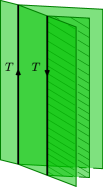
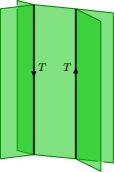
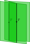
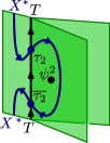
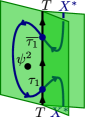
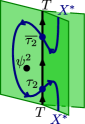
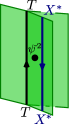
Let be a defect bordism, and let be two parallel -strata, connected by a -stratum . Denote the multimodule which labels by and the algebra which labels by (see Figure 1(a)). Upon ribbonisation, gets replaced by a ribbon graph connecting and , which upon evaluation with can be replaced by the idempotent (2.13), projecting onto . The same result can be obtained by replacing and with a single -stratum labelled with (see Figure 1(b)). If end on the boundary or on -strata in , the endpoints also need to be relabelled. In this case, a cylinder as in Figure 1(c) provides an isomorphism between the surfaces with different decorations.
Property 3.8.
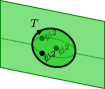
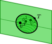
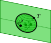
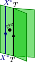
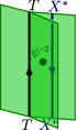
The set of labels for -strata lying in a -stratum labelled with an algebra is given by bimodule maps : By definition it is the vector space assigned to a stratified -sphere surrounding the -stratum and having a single -coloured loop. Its cylinder and a choice for its ribbonisation are depicted in Figures 2(a) and 2(b). By Property 3.3, the Reshetikhin–Turaev TQFT assigns the space to the -sphere with two -coloured punctures such that an element corresponds to a closed ball with an embedded -labelled coupon and two -strands. The image of is then a closed ball with an embedded ribbon graph as in Figure 2(c). The two -lines on the sides of the coupon act precisely as the projection .
An analogous argument for -strata separating two -strata labelled with multimodules yields that they are labelled with multimodule morphisms (see [8, Lem. 3.1]). This also implies that two -strata which are connected by a -stratum can be composed, e. g. for three multimodules and multimodule morphisms , one has
| (3.28) |
Similarly, the -strata within the same -stratum can also be composed.
Property 3.9.
Let be a -stratum labelled with an algebra , which is bounded by -strata labelled by multimodules (and by some -strata between them). Let be a 0-stratum adjacent to no 2-stratum other than , labelled by a bimodule morphism . Assume that is contractible, as illustrated on the left-hand side of Figure 3.3. Then, upon evaluation with , can be removed with pushed aside to form a -stratum on one of the bounding 1-strata, for example the one labelled with , and relabelled with the where or (recall the notation (2.17)), depending on which action of on is used. The action of on is forgotten afterwards to make them into valid labels once is removed. This is summarised in Figure 3.3, where . To show this identity, one uses the properties of -separable symmetric Frobenius algebras and their modules to simplify the ribbon graph that replaces after ribbonisation.
3.3 Orbifold graph TQFT
Let be a modular fusion category, let be a simple orbifold datum in it, and consider the associated modular fusion category (see Section 2.3). We are now ready to define the Reshetikhin–Turaev orbifold graph TQFT555In the notation of [3], would be denoted as .
| (3.29) |
Orbifold graph TQFTs were introduced in [3] as graph TQFTs obtained by performing an internal state sum construction in a given -dimensional defect TQFT. Our construction is a generalisation of the state sum TQFT in [21] which one recovers in the special case . In this section we specialise the general construction in [3] to the case of the Reshetikhin–Turaev defect TQFT from Section 3.2. We refer to [3] for more details on orbifold graph TQFTs.
Orbifold datum as defect labels
The defect TQFT allows one to interpret the orbifold datum as a set of distinguished defect labels (see Figure 3.4): The label for a -stratum, for a -stratum having three adjacent -strata labelled by , and for the “intersection” points of four -labelled -strata, for -strata on -labelled -strata, and for -strata inside -strata. The identities in Figure A.1 then can be interpreted graphically as depicted in Figure 2(a), where each identity corresponds to a local change on the appropriately labelled defect configuration that can be performed upon evaluation with without changing the resulting invariant.
An object can also be interpreted as a collection of defect labels (see Figure 3.5): The label for a -stratum lying within an -labelled -stratum and , for the “intersection” points of - and a -labelled -strata. The algebraic identities in Figure 3(a) then correspond to changes of defect configurations as in Figure A.4.
Ribbon diagrams and foamification
The graph TQFT is based on the “foamification” map
| (3.30) |
which is an analogue of the ribbonisation map (3.19) used to define the defect TQFT . In particular, will not be a functor.
Let be a -manifold with an embedded -coloured ribbon graph . We denote the underlying unlabelled ribbon graph by . The following notions are taken from [3] (and are in turn based on the analogous notions in [21]).
-
•
An admissible -skeleton for is a stratification dividing into a finite collection of open balls and (in case has boundary) half-balls, such that each point has a neighbourhood isomorphic to one of the stratified spaces depicted in Figure 3.4 (at this point unlabelled). Here , denotes the union of strata of with dimension . The qualifier “admissible” refers to the orientations of the strata, which are as in Figure 3.4 with the points labelled by / having the orientation . Note that an admissible -skeleton on induces an admissible -skeleton on .
-
•
An admissible positive ribbon diagram for is an admissible -skeleton for together with an embedding , which is isotopic to the identity embedding and such that all strands/coupons lie in the -strata with framings induced by their orientations, except for finitely many intersection points between the strands of and -strata, which have neighbourhoods isomorphic to one of the stratified spaces in Figure 3.5 (at this point unlabelled). The qualifier “positive” refers to the orientations imposed by Figure 3.5.
Since the skeleta and ribbon diagrams we consider below are always admissible (and positive), we omit mentioning “admissible” and “positive” below.
-
•
An -coloured ribbon diagram for is a ribbon diagram with the following labels assigned:
-
–
- and -strata of are labelled with and , -strata of by or as in Figure 3.4;
-
–
the intersection points of the -strata of with strand of that is labelled with are labelled with or as in Figure 3.5;
and the following -strata added:
-
–
for a -stratum of , each component of gets an additional -stratum labelled with where
(3.31) is the symmetric Euler characteristic; the boundary segments of coupons are treated as boundary components of ;
-
–
the 2-strata adjacent to the left and the right edges of each coupon get an additional -insertion;666As explained in [3, App. B], these additional -insertions are needed so that the coupons of the embedded ribbon graphs can be composed when evaluating with the orbifold graph TQFTs.
-
–
each -stratum of gets an additional -stratum labelled with .
-
–
An -coloured ribbon diagram for can be seen as a stratification for consisting of together with additional - and -strata obtained from the embedding as well as the - and -insertions. On the boundary it restricts to an -coloured -skeleton of punctured surfaces, i. e. a -skeleton with additional -strata at the punctures.
For a -coloured surface , pick an -coloured 1-skeleton . We define the foamification of ,
| (3.32) |
to be a defect surface obtained from the underlying surface with the stratification and labels as in .
For a -coloured ribbon bordism , let be an -coloured ribbon diagram. The foamification
| (3.33) |
of is defined to be the defect bordism with the stratification given by and restricting to the -skeleta of punctured surfaces on the boundary components .
Reshetikhin–Turaev orbifold graph TQFT
We define the orbifold graph TQFT in terms of the Reshetikhin–Turaev defect TQFT (see Section 3.2) in a way similar to the definition of the latter in terms of the Reshetikhin–Turaev graph TQFT (see Section 3.1). The construction is based on the following result (see [3, Cor. 4.13]).
Theorem 3.10.
Let be a -coloured ribbon bordism and let be two -coloured ribbon diagrams which agree on the boundary components . Then
| (3.34) |
From here on we proceed similarly as in Section 3.2, following [3, Sect. 4.3.2]. For two -decorated skeleta of a punctured surface , let be an -decorated ribbon diagram of the cylinder bordism which restricts to and on the incoming and outgoing boundaries, respectively. Define the linear map
| (3.35) |
By Theorem 3.10 it is independent of the stratification in the interior and hence the following equality holds for all -decorated skeleta of the punctured surface :
| (3.36) |
Construction 3.11.
Let be a simple orbifold datum in a modular fusion category . The orbifold graph TQFT
| (3.37) |
is defined as follows:777This construction works in the same way if is not simple. The only change is that is multifusion. Since here we are concerned with the case that is again a modular fusion category, we prefer not to switch between simple and not necessarily simple in the presentation.
-
(i)
For an object we set
(3.38) where range over -decorated skeleta of the punctured surface .
-
(ii)
For a morphism we set to be
(3.39) where is an arbitrary -decorated ribbon diagram of restricting to on the boundary components .
As in (3.27), the state spaces of are isomorphic to the images of the idempotents ,
| (3.40) |
Let us collect some useful properties of .
Property 3.12.
The orbifold graph TQFT (like the graph TQFT , see Section 3.1) is a regular graph TQFT, i. e. the moves in (3.12) become identities upon evaluation.888 This as well as Property 3.13 actually hold in general for the graph TQFTs of [3], but we only use them here for . This follows from Property 3.8 of the defect TQFT . Indeed, upon choosing an -coloured ribbon diagram and evaluating with , without loss of generality one can assume e. g. that the two coupons being composed lie in the same -labelled -stratum and interpret them as -strata labelled by the corresponding --bimodule morphisms. There is an additional complication due to the -insertions needed in the -colouring of a ribbon diagram, but the composition of the -strata still remains the same as for bimodule morphisms. In fact, the requirement to add a -insertion to the left and to the right of each coupon was made to ensure that this holds, see [3, App. B].
Property 3.13.
Consider an -coloured ribbon diagram obtained from the foamification procedure. If contains a strand labelled by an object obtained from applying the pipe functor (2.31) to a bimodule , we can exchange this strand for a pipe made of -labelled -strata with an -labelled line in the middle (see Figure 6(a)) without changing the value of the defect TQFT . Similarly, coupons labelled with braiding morphisms involving the object can be exchanged for stratifications as depicted in Figures 6(b) and 6(c).
Example 3.14.
Let and let be the morphism in represented by the -sphere with a single embedded -labelled coupon. Since is the tensor unit in , the coupon does not need to have adjacent strands, see Figure 7(a). We compute the invariant . Let be an -decorated ribbon diagram for consisting of an embedded -sphere containing the coupon. The resulting foamification is depicted in Figure 7(b). The defect sphere becomes a closed disc after removing the coupon; since the edges are treated as its boundary components, its symmetric Euler characteristic as given by (3.31) is , which explains the -insertion. The other two -insertions are the ones that each coupon gets to the left and to the right of it. has two -strata (the “inside” and the “outside” of the defect sphere), each of which gets a -insertion.
Next we consider the ribbonisation where is the -skeleton of the defect sphere with point insertions as shown in Figure 7(c). Using the invariant (3.14) of one obtains:
| (3.41) |
where in the third equality we collected the -insertions into a single prefactor and simplified the ribbon graph into an -labelled loop with an insertion. Since is simple, one can identify the scalar with the trace . Applying the expression (2.27) then yields
| (3.42) |
The resulting invariant is therefore precisely . In fact, since any -coloured ribbon graph in can be simplified into a single coupon, this shows that more generally the equality
| (3.43) |
holds. In Section 4.2 this will play a role in showing that the two graph TQFTs are isomorphic. Note that at this point we have not yet shown that the invariants of for an arbitrary are equal as we have not shown that the anomalies of and coincide, see (3.8). This is done in Lemma 4.5 below.
Example 3.15.
Let be the -sphere with a single labelled puncture. We compute the vector space . Let be the -coloured ribbon diagram of the cylinder restricting to a -skeleton on the boundary as depicted in Figure 8(a), and let
| (3.44) |
be the corresponding foamification. By definition one has
| (3.45) |
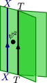
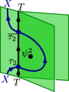
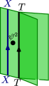
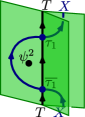
The vector space can be identified with by sending an --bimodule morphism to where is the stratified closed ball bordism as in Figure 8(b).999 Since is a linear map from to , we should write , but will usually keep the argument implicit. One has the equality
| (3.46) |
where is the averaged morphism introduced in (2.29). Indeed, corresponds to the evaluation which can be computed by ribbonising the argument and rearranging the result as in Figure 8(c) (for that we use the notation (2.17) and the crossing morphisms for (2.21)). We conclude that for a simple orbifold datum one has
| (3.47) |
Note that for a morphism , the defect bordism is a choice of foamification of the bordism as introduced in (3.13).
4 Proof of isomorphism
Let be a simple orbifold datum in a modular fusion category . From this we obtain the modular fusion category (cf. Section 2.3) and the associated Reshetikhin–Turaev TQFT (Section 3.1). In this section we prove that this is the orbifold graph TQFT of Section 3.3, hence showing that Reshetikhin–Turaev theories close under orbifolds:
Theorem 4.1.
Let be a simple orbifold datum in a modular fusion category . Then the orbifold graph TQFT for the choice of square root is equivalent (as monoidal functors) to the graph TQFT for the choice of square root as in (2.27). Moreover, the monoidal natural isomorphism is unique.
The proof is similar to that of the isomorphism between the TQFTs of Turaev–Viro type obtained from a spherical fusion category with and the Reshetikhin–Turaev TQFTs obtained from the Drinfeld centre , see [21, Ch. 17]. It relies on the following technical lemma, cf. [21, Lem. 17.2]. Since the uniqueness part of the statement is not part of the statement in loc. cit. we repeat the main idea of the proof.
Lemma 4.2.
Let be a rigid monoidal category and let be monoidal functors where we assume without loss of generality that . Moreover, suppose that
-
i)
is non-degenerate, i. e. for all objects one has
(4.1) -
ii)
for all one has
(4.2) -
iii)
for all one has
(4.3)
Then there is a unique natural monoidal isomorphism between and .
Proof.
Suppose is a natural transformation. For all and all , by naturality of the diagram
| (4.4) |
commutes. Since by assumption the vectors span , this requirement determines uniquely. In the proof of [21, Lem. 17.2] it is shown that defining by the diagram (4.4) yields a well-defined monoidal natural transformation that has an inverse due to the assumption in part ii. ∎
Proof of Theorem 4.1.
Note that for condition ii follows form condition iii, since for all , the invariant of already yield the dimension of the corresponding state space, see (3.17). The more involved argument in Section 4.3 is needed to cover also the case .
4.1 Skeleta from surgery
Let be a closed connected -coloured ribbon -manifold with an embedded ribbon graph . For a choice of surgery link for we construct an -coloured ribbon diagram for :
-
i)
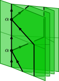
Following Section 3.1, let be the ribbon graph in representing i. e. consisting of possibly linked components of and such that surgery along yields . Project on the outwards oriented unit -sphere in so that the coupons do not intersect the strands, the intersections of strands are pairwise distinct and transversal, and the framings of components of agree with the orientation of the -sphere. The intersection points are marked to distinguish between “overcrossings” and “undercrossings”. For simplicity we assume that there are no crossings between the strands of , which can be achieved by exchanging them with coupons labelled with braiding morphisms. We identify and with their projection images in just described.
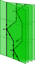
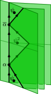
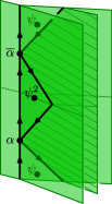
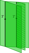
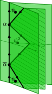
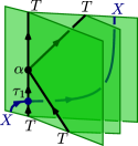
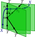
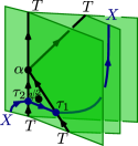
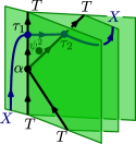
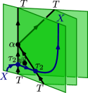
(a) (b) (c) (d) Figure 4.1: Exchanging surgery lines with tubes. Each -stratum has the paper plane orientation, -strata have orientations as indicated. In our application, strands that belong to the ribbon graph will carry a label of some object , red strands will carry the Kirby object (3.5), black strands will carry the label from the orbifold datum . Vertices will be labelled by , from or by the crossing morphisms from , as appropriate. (a) (b) (c) Figure 4.2: For each component , the 3-strata , in the interior of the surrounding pipe become contractible after surgery. The pictures only show a strip of the pipe: it is actually closed and can be adjacent to other 2-strata or the strands of (which are ignored in this illustration). The inner white tube represents the solid torus with the two meridian disks , , that is being glued along during surgery (for this tube the top and the bottom can be thought of as identified). Moreover, maps the boundaries of the discs , in to the meridian lines on the boundary of the solid torus. The pictures (a), (b) and (c) all depict the same configuration, in (b) and (c) the pipe stratification is moved inside the solid torus along . -
ii)
Surround each strand of by additional - and -strata as shown in Figure 1(a). As we will see later, this is done intentionally to mimic the stratification corresponding to a “pipe” object of as explained in Section 3.1. The crossings between the components of and are exchanged for the stratifications as in Figures 1(b) and 1(c), analogous to those corresponding to the braiding morphisms involving the pipe objects. The crossings between the components of are handled in the same way, which results in a more intricate stratification shown in Figure 1(d).
At this point, the 3-strata in the stratification of are given by two open balls, and by two open tori for each component of .
-
iii)
Perform surgery along (see Section 3.1): for each component of let be a tubular neighbourhood of it, which lies inside the pipe stratification and let be the diffeomorphism along which the gluing with a solid torus is performed, i. e. such that coincides with the framing of . We make this into a gluing of two stratified manifolds as follows: Provide the solid tori with stratifications by two oriented meridian discs
(4.5) Since the -strata on run parallel to the curve left by the framing of , we can assume that is an isomorphism of stratified surfaces, i. e. maps to the -strata of , see Figure 2(a). This yields the manifold together with a stratification , whose strata (besides those belonging to ) are unlabelled.
-
iv)
To show that is a ribbon diagram for , one needs to argue that all its -strata are contractible. The two 3-strata of given by open balls do not intersect the tubular neighbourhoods and are not affected by the surgery. For the 3-strata that were open tori before surgery we proceed as follows:
For a component of , let be the -strata inside the pipe stratification added in step ii. Before the surgery, and are homeomorphic to open solid tori. After the surgery their topology is changed: one can move the pipe stratification together with across the diffeomorphism into the interior of the solid torus where they look like open solid cylinders and are evidently contractible (see Figures 2(b) and 2(c)). -
v)
Define the -coloured ribbon diagram by labelling the strata of as in Section 3.3: the -strata with , the -strata either with or with the label of the corresponding strand of , and the -strata either with /, with the morphisms labelling the coupons of , or with the crossings morphisms between the -lines and the strands of . Finally, add the appropriate - and -insertions.
The number of -strata in the ribbon diagram is , where is the number of components of . Indeed, the -sphere in step i creates two -strata and for each component of the pipe stratification creates two more -strata.
4.2 Invariants of closed 3-manifolds
Let be a connected -coloured ribbon -manifold and let be a choice of surgery link for . Let be the -coloured ribbon graph in obtained from by colouring each component of with and adding a -insertion, as well as exchanging the crossings with braiding morphisms.
Lemma 4.3.
The following formula holds:
| (4.6) |
where since is a simple orbifold datum, one has .
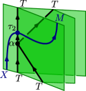
Besides the general proof below, we illustrate some steps in the proof of Lemma 4.3 in Figure 4.3 for the explicit example of the invariant of the ribbon -manifold , for which we use the surgery link having one component with a single twist, i. e.
| (4.7) |
This example will later help us compute the anomaly of the category .
Proof of Lemma 4.3.
In terms of the -decorated ribbon diagram from Section 4.1, by definition of the invariants of closed manifolds one has
| (4.8) |
where is the foamification discussed in Section 3.3. We apply the properties of the defect TQFT as reviewed in Section 3.2 to modify the stratification of in several steps:
-
i)
For each component of , the meridian discs of the solid tori glued in during surgery (i. e. as in (4.5)) are part of contractible -strata of each of which has a -insertion as given by (3.31). From Section 3.2 we know that they can be removed with the -insertions moved aside to give -insertions on the adjacent -labelled -strata (recall Property 3.9 and (2.17)). The rest of can then be moved so as to not intersect the boundaries of the solid tori along which the surgery was performed.
-
ii)
We can now undo the surgery used to obtain , that is, we replace with and embedded surgery link with in the complement of . By definition of via the Reshetikhin–Turaev TQFT and the formula (3.16) for the invariants of closed manifolds, one can further proceed by replacing the link with its coloured version (i. e. with components labelled by and having -insertions, see (3.5) and (3.6)) and multiplying with the overall factor . If for the example surgery link in (4.7) we choose the projection to depicted in Figure 4.3a, the resulting stratification of is as shown in Figure 4.3b.
-
iii)
Following Section 3.3, the components of the labelled surgery link , along with the pipe stratifications surrounding them, can be exchanged for the -strata labelled by the objects , i. e. by the pipe objects obtained from the induced bimodule . As an intermediate step in this change one uses the isomorphisms of --bimodules in order to apply the definition (2.31) with . surrounding stratification obtained in step i can be collected into a single -insertion. The stratifications that replaced the crossings of strands in the construction of (i. e. the ones depicted in Figures 1(b), 1(c) and 1(d) with the appropriate -insertions) can in turn be replaced with coupons labelled by the braiding morphisms.
-
iv)
The previous step yields an overall factor (which previously served as -insertions for the -strata inside the pipe stratifications surrounding the components of ) and simplifies the stratification of to an -labelled -sphere with the graph projected on it as well as the two remaining -insertions in its -strata (see Figure 4.3c for how it looks for the example surgery link ). The ribbon graph can be further exchanged for a single coupon labelled with . At this point one recognises the remaining stratification of as the ribbon diagram used in Example 3.14. Using the computation (3.42) and collecting all prefactors, one obtains the formula (4.6).
∎
We proceed to compare the expression (4.6) with the invariant , which is obtained by adapting (3.8) for the modular fusion category . We start by addressing the different colourings of the surgery link.
Let be any morphism in the category of -coloured ribbon graphs (for the sake of generality, we do not assume that is closed, i. e. it can have free incoming/outgoing strands), and let be an uncoloured oriented framed link. Denote as before by a ribbon graph consisting of possibly entangled components of and and by and its versions with carrying the respective colouring by objects and with additional point insertions labelled by the endomorphisms and .
Lemma 4.4.
One has the following identity of morphisms in :
| (4.9) |
Proof.
We will need the following decompositions for simple objects , , (the label above the isomorphism symbol indicates the category in which it holds):
| (4.10) |
For the isomorphisms c) and d) we used that the pipe functor and the induction functor are biadjoint to the respective forgetful functors.
For a simple object and a morphism , let us denote by the number such that .
It is enough to show (4.9) for the case when has one component, i. e. , as one can then iterate the argument. For an object and a morphism , let be the colouring of by with an -insertion so that
| (4.11) |
In addition we abbreviate and . One has:
| (4.12) |
∎
The identity in Lemma 4.4 provides the penultimate step in comparing the invariants of closed ribbon -manifolds. We apply it first to compare anomalies (defined in (2.10)):
Lemma 4.5.
For the choice of square roots of global dimensions related as in (2.27), the modular fusion categories and have the same anomaly: .
Proof.
We compare two computations of the invariant , one using the empty surgery link as in the Example 3.14 and the other using the surgery link in (4.7). The former one is obtained from (3.43) and (3.14) and gives . For the latter, note that one has and it follows from (2.9) that . One uses Lemmas 4.3 and 4.4 to compute:
| (4.13) |
Since by well-definedness of the two computations have to agree, the statement follows. ∎
Lemma 4.6.
Let be a closed -coloured ribbon -manifold viewed as a morphism in . One has:
| (4.14) |
Proof.
Since both invariants are multiplicative with respect to connected components, it is enough to consider the case when is connected. One has:
| (4.15) |
∎
4.3 State spaces
In this section we will show condition ii in Lemma 4.2, that is the inequality for a punctured surface . To do this, we first give an explicit description of the TQFT state spaces on both sides of the inequality.
It is enough to consider the case of having a single labelled puncture (this follows from [21, Lem. 15.1] and the regularity of both TQFTs, see Properties 3.2 and 3.12). In Example 3.14 we already looked at the case when has genus 0 so here we will assume to have genus .
The vector spaces assigned to punctured surfaces by the Reshetikhin–Turaev TQFT were already mentioned in Property 3.3. For the genus- surface with an -labelled puncture one has, with ,
| (4.16) |
where the direct sum is over . Explicitly, the overall isomorphism is given by
| (4.17) |
Here is the ribbon bordism , diffeomorphic to the solid genus- handlebody and having the following ribbon graph lying at its core:
| (4.18) |
where each of the handles is depicted by a vertical cylinder with top and bottom identified.
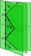
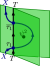
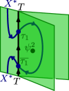
We now turn to computing the state space , for which we will use the formula (3.40). To this end, let be the -coloured ribbon diagram for the cylinder as depicted in Figure 4.5, where a similar presentation as that of the ribbon handlebody in (4.18) is used: is represented by a closed solid genus- handlebody with an open solid handlebody removed from its interior; each of the handles is depicted as a vertical cylinder over an annulus with identified top and bottom. To arrive at the ribbon diagram we proceed in four steps, the first three of which are illustrated in Figure 4.5, where we show only the part involving the leftmost handle:
-
•
one starts by adding to vertical -labelled -strata connecting the boundary components as shown in Figure 4(a);
-
•
the two boundary components are then separated by further stratification with -labelled 2-strata, -labelled 1-strata, and 0-strata labelled with appropriate crossing morphisms of , resembling the one in the definition of the pipe functor as shown in Figure 4(b);
-
•
one adds the horizontal -labelled strata as in Figure 4(c), to make all -strata contractible;
-
•
the - and -insertions in are as in the definition of an -coloured ribbon diagram: in our present case all -strata are contractible, so those that touch the boundary receive a -insertion and those that do not receive a -insertion; there are four -strata, all of which touch the boundary and therefore receive a -insertion.
Let be the -coloured 1-skeleton of the punctured surface , obtained by restricting the ribbon diagram to its incoming (or equivalently outgoing) boundary. Denote the foamifications of and by and , respectively. We need to compute the image of the idempotent
| (4.19) |
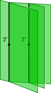
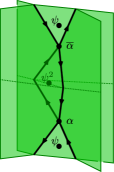
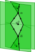
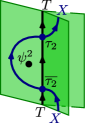
As an intermediate step one therefore needs to know the vector space . To this end, let be the solid defect genus- handlebody depicted in Figure 6(a), seen as a defect bordism , with the lines labelled by --bimodules and the points by --bimodule morphisms
| (4.20) |
and --bimodule morphisms
| (4.21) |
Lemma 4.7.
The vector space is spanned by elements of the form .
Proof.
As described in Construction 3.6, the state space is the image of the idempotent acting on as in (3.27). In the present case, is given by applying to the bordism in Figure 6(b). Acting on a spanning set of the state space in terms of handlebodies with ribbon graphs along their core (similar to (4.18), but for and with -insertions in addition to the -insertion) results in the handlebody shown in Figure 6(c). This effectively replaces the objects by the induced bimodules , , …. One verifies that the morphisms get mapped to morphisms commuting with -actions as required by the defect bordism in Figure 6(a) (but with replaced by , etc.). Expanding the induced bimodules into simple bimodules shows the claim. ∎
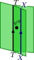
By the previous lemma, the image of is spanned by vectors of the form
| (4.22) |
The defect handlebody in the argument of on the right-hand side of (4.22) is shown in Figure 6(d), where, as in Figure 4.5, only the first handle is depicted. Using the pipe functor , the stratification inside the handlebody can be exchanged for the one depicted in Figure 6(e) without changing the value under . Here the points are labelled by morphisms
| (4.23) | ||||
| (4.24) |
all of which satisfy (2.18) and are therefore morphisms in . By the semisimplicity of , one can decompose into a linear combination of handlebodies with stratification as in Figure 6(f), where – using the same labels as in (4.18) – are simple objects of , and and are morphisms in .
Denote the handlebody in Figure 6(f) by . Then, in summary, is spanned by vectors of the form .
Lemma 4.8.
One has
| (4.25) |
Proof.
This completes the proof of Theorem 4.1.
Appendix A Defining identities
(O1)
(O2)
(O3)
(O4)
(O5)
(O6)
(O7)
(O8)

(O1)
(O2)
(O3)
(O4)
(O5)
(O6)
(O7)
(O8)
(T1)
(T2)
(T3)
(T4)
(T5)
(T6)
(T7)
(T1)
(T2)
(T3)
(T4)
(T5)
(T6)
(T7)
 ,
, 
 ,
, 
 ,
, 
 ,
, 
Appendix B Pipe functors
Throughout this section we fix a 3-dimensional defect TQFT over defect data and we also fix an orbifold datum for (which does not need to be simple).101010We assume in this appendix that is an Euler-complete TQFT in order to avoid - and -insertions. However this is not really a limitation as for an arbitrary 3-dimensional defect TQFT this can always be achieved by passing to its “Euler completion” ; see also [3, Appendix B]. In this section we describe the pipe functors , where and are the monoidal categories associated to and in [3, Sect. 4.2]. In the case where is the Reshetikhin–Turaev TQFT and is the kind of orbifold data considered in [18] the construction we present here specialises to the pipe functors introduced in [18, Sect. 3.3], cf. (2.30). The objects of are decorated lines that live on an -decorated plane and the category has as objects triples where and are isomorphisms that let an -decorated line pass through decorated lines. For the construction of , we introduce two intermediate categories , . The former has as objects tuples where is an object of and is an isomorphism
| (B.1) |
We require that , satisfy the equations (T1) and (T4)–(T7) from [3, p. 40]. Similarly has as objects tuples where and is an isomorphism
| (B.2) |
satisfying (T1) and (T4)–(T7) from [3, p. 40]. One obtains a strictly commuting diagram of forgetful functors
| (B.3) |
We now construct the “half-pipe” functors
| (B.4) |
which will turn out to form biadjunctions with the respective forgetful functors, satisfying a separability condition. For we set
| (B.5) |
It can be readily checked that indeed endows with the structure of an object of . is defined similarly, except that each picture is reflected at the paper plane so that the half-pipe is added in the back:
| (B.6) |
acts in the same way as , by adding a half-pipe in the front. For any this equips with a analogously to the case of , so that we indeed end up with an object of . Entirely analogously, acts as does.
Proposition B.1.
For each , the functor is biadjoint to the corresponding forgetful functor, thus giving rise to two Frobenius monads and . Each is separable. Let and . The unit and counit of the adjunction are given in components by
| (B.7) |
and the unit and counit of the adjunction by
| (B.8) |
The units and counits for the other adjunctions are obtained similarly.
Proof.
We check the necessary identities for the adjunctions involving . The remaining cases are similar and we leave them to the reader. To see that we calculate
| (B.9) |
In step (1) we first drag the end of the inner pipe upwards along the outside of the inner pipe. We then attach it to the inside of the outer pipe using the defining equations for orbifold data, arriving at the second picture. In step (2) we pop the -decorated bubble as indicated, which is again possible by using the axioms of orbifold data. Furthermore we have
| (B.10) |
In step (1) we use the compatibility of with from the orbifold datum, step (2) is a matter of plugging in the definition of dual morphisms, while step (3) follows from and the fact that -decorated bubbles can be removed.
To see that we have to show that and . Both identities follow pictorially very similarly as above, only that the pictures are rotated by 180° around the axis that is orthogonal to the paper plane and the orientation of - and -decorated lines is reversed.
Finally, the separability of the Frobenius monad follows from
| (B.11) |
∎
Definition B.2.
The pipe functors are given by and . They act by
| (B.12) |
It follows from the above proposition that both and are biadjoint to the forgetful functor where the units and counits are obtained by composing the corresponding ones of the halfpipe functors. There is a unique isomorphism that is compatible with the biadjunction data and one verifies that it is given in components by
| (B.13) |
References
- [1] C. Blanchet, N. Habegger, H. Masbaum, and P. Vogel, Topological quantum field theories derived from the Kauffman bracket, 10.1016/0040-9383(94)00051-4Topology 34:4 (1995), 883–927.
- [2] B. Bakalov and A. Kirillov, Lectures on tensor categories and modular functors, 10.1090/ulect/021University Lecture Series 21, AMS, 2001.
- [3] N. Carqueville, V. Mulevičius, I. Runkel, D. Scherl, and G. Schaumann, Orbifold graph TQFTs, arXiv:2101.02482 [math.QA].
- [4] N. Carqueville, C. Meusburger, and G. Schaumann, 3-dimensional defect TQFTs and their tricategories, 10.1016/j.aim.2020.107024Adv. Math. 364 (2020) 107024, arXiv:1603.01171 [math.QA].
- [5] N. Carqueville, I. Runkel, Rigidity and defect actions in Landau-Ginzburg models, 10.1007/s00220-011-1403-xCommun. Math. Phys. 310 (2012) 135–179, arXiv:1006.5609 [hep-th].
- CRS [1] N. Carqueville, I. Runkel, and G. Schaumann, Orbifolds of -dimensional defect TQFTs, 10.2140/gt.2019.23.781Geometry & Topology 23 (2019), 781–864, arXiv:1705.06085 [math.QA].
- CRS [2] N. Carqueville, I. Runkel, and G. Schaumann, Line and surface defects in Reshetikhin–Turaev TQFT, 10.4171/QT/121Quantum Topology 10 (2019), 399–439, arXiv:1710.10214 [math.QA].
- CRS [3] N. Carqueville, I. Runkel, and G. Schaumann, Orbifolds of Reshetikhin–Turaev TQFTs, Theory and Applications of Categories 35 (2020), 513–561, arXiv:1809.01483 [math.QA].
- [9] M. De Renzi, A. M. Gainutdinov, N. Geer, B. Patureau-Mirand, and I. Runkel, 3-Dimensional TQFTs from Non-Semisimple Modular Categories, arXiv:1912.02063 [math.GT].
- [10] A. Davydov, M. Müger, D. Nikshych, and V. Ostrik, The Witt group of non-degenerate braided fusion categories, 10.1515/crelle.2012.014J. reine und angew. Math. 677 (2013) 135–177, arXiv:1009.2117 [math.QA].
- [11] P. I. Etingof, S. Gelaki, D. Nikshych, and V. Ostrik, Tensor categories, Math. Surveys Monographs 205, AMS, 2015.
- FRS [1] J. Fuchs, I. Runkel, and C. Schweigert, TFT construction of RCFT correlators. 1: Partition functions, 10.1016/S0550-3213(02)00744-7Nucl. Phys. B 646 (2002) 353–497, arXiv:hep-th/0204148.
- [13] J. Fuchs, C. Schweigert, and A. Valentino, Bicategories for boundary conditions and for surface defects in 3-d TFT, 10.1007/s00220-013-1723-0Communications in Mathematical Physics 321:2 (2013), 543–575, arXiv:1203.4568 [hep-th].
- [14] D. Gaiotto and T. Johnson-Freyd, Condensations in higher categories, arXiv:1905.09566 [math.CT].
- [15] P. M. Gilmer and X. Wang, Extra structure and the universal construction for the Witten–Reshetikhin–Turaev TQFT, 10.1090/S0002-9939-2014-12022-3Proc. Amer. Math. Soc. 142 (2014), 2915–2920, arXiv:1201.1921 [math.GT].
- [16] V. Koppen, V. Mulevičius, I. Runkel, and C. Schweigert, Domain walls between 3d phases of Reshetikhin-Turaev TQFTs, arXiv:2105.04613 [hep-th]
- [17] A. Kapustin and N. Saulina, Surface operators in 3d Topological Field Theory and 2d Rational Conformal Field Theory, Mathematical Foundations of Quantum Field Theory and Perturbative String Theory, Proceedings of Symposia in Pure Mathematics 83, 175–198, American Mathematical Society, 2011, arXiv:1012.0911 [hep-th].
- [18] V. Mulevičius and I. Runkel, Constructing modular categories from orbifold data, arXiv:2002.00663 [math.QA].
- [19] V. Mulevčius, Condensation inversion and Witt equivalence via generalised orbifolds, in preparation.
- [20] V. Turaev, Quantum invariants of knots and 3-manifolds, de Gruyter, 2010, 2nd edition.
- [21] V. Turaev and A. Virelizier, Monoidal Categories and Topological Field Theory, 10.1007/978-3-319-49834-8Progress in Mathematics 322, Birkhäuser, 2017.