Dynamical-systems theory of cellular reprogramming

Abstract

In cellular reprogramming, almost all epigenetic memories of differentiated cells are erased by the overexpression of few genes, regaining pluripotency, potentiality for differentiation. Considering the interplay between oscillatory gene expression and slower epigenetic modifications, such reprogramming is perceived as an unintuitive, global attraction to the unstable manifold of a saddle, which represents pluripotency. The universality of this scheme is confirmed by the repressilator model, and by gene regulatory networks randomly generated and those extracted from embryonic stem cells.

In the development of multicellular organisms, cells with identical genomes differentiate into distinct cell types. This cellular differentiation process has often been explained as balls falling down the epigenetic landscape, as originally proposed by Waddington Waddington (1957): balls start from the top of the landscape, and as development progresses, they fall into distinct valleys, which correspond to differentiated cell types. In modern biology, such landscapes are believed to be formed by epigenetic regulation, including DNA and chromatin modificationsBird (2007); Goldberg et al. (2007); Cortini et al. (2016); Surani et al. (2007). For pluripotent cells, these modifications are small, whereas each differentiated cell type has a different epigenetic modification pattern Meshorer et al. (2006); Atlasi and Stunnenberg (2017); Mikkelsen et al. (2007); Tripathi and Menon (2019). Cells with pluripotency, such as embryonic stem (ES) cells, are located in the vicinity of the first branching point into the valleys, because they can easily differentiate into different types of cells with just slight stimuli Levenberg et al. (2002).

In 2006, a seminal study by Takahashi and Yamanaka reported that differentiated cells can regain pluripotency only by overexpressing few genes (so-called the four Yamanaka factors) without direct manipulations of epigenetic modifications. This was termed as reprogramming of induced pluripotent stem (iPS) cells Takahashi and Yamanaka (2006). The reprogramming is often described as “climbing” the epigenetic landscape Takahashi and Yamanaka (2016); Hochedlinger and Plath (2009); Velychko et al. (2019). This hypothesis, however, has two problems that still need to be addressed: (1) cells have many degrees of freedom, with expression and epigenetic modifications of many genes, whereas reprogramming manipulation involves only few degrees of freedom. How is it possible?; moreover, (2) if the initial pluripotent state is represented by the top of the landscape, it is not a stable point. Thus, how can reprogramming robustly make the cells head toward such an “unstable” state?

Theoretically, these issues should be resolved based on dynamical systems theory. The interplay between fast gene regulation and slow epigenetic dynamics shapes the epigenetic landscape, and differentiated cells are represented by different attractors Kauffman (1969); Wang et al. (2010); Forgacs and Newman (2005, 2005). Therefore, upon the reprogramming operation, cellular states starting from different attractors first converge into a unique pluripotent state, which is not stable, from which states move toward various attractors afterwards. At first glance, these requirements seem to be incompatible; an unstable state (e.g., repeller) is not attracted from different initial conditions. Hence, to satisfy these requirements, the pluripotent cell is expected to be represented at least by a saddle that is attracted from many directions and departs only along unstable directions (manifolds), which represent the cell differentiation process, leading to attractors of different destinations. To regain pluripotency by reprogramming, cellular states must be placed on the stable manifold of the saddle by common manipulations from different attractors. Such manipulation, however, would require fine-tuned control. In contrast, reprogramming is mediated by the overexpression of a few common genes across a variety of differentiated cell types. Therefore, some dynamical systems concept beyond just a saddle is needed.

A recent experiment provides some clues on this subject. Temporal oscillations in DNA methylation and corresponding gene expression levels are observed during cellular differentiation Rulands et al. (2018); Kangaspeska et al. (2008). In fact, gene expression oscillations have also been reported during somitogenesis and in embryonic stem cells Palmeirim et al. (1997); Kobayashi et al. (2009); Canham et al. (2010), whereas its relevance to cell differentiation has been theoretically investigated for decades Furusawa and Kaneko (2012); Ullner et al. (2008); Koseska et al. (2010); Suzuki et al. (2011); Koseska et al. (2013); Goto and Kaneko (2013); Miyamoto et al. (2015). Recalling possible significance of oscillatory dynamics, it is reasonable to consider that if there is an oscillation of fast gene expression around the saddle point of the slow epigenetic dynamics, global attraction to it from broad initial conditions may be attained beyond its stable manifold. As the oscillation dynamics are extended beyond the stable manifold of a saddle, global attraction to the vicinity of the saddle may be possible by taking advantage of the interplay between fast expression and slow modification dynamics.

Herein, we verified this possibility by using a dynamical system model with a gene regulatory network (GRN) and epigenetic modification. We consider a cell model in which the cellular state was represented by the expression $x_{i}$ and epigenetic modification level $\theta_{i}$ for each gene $i$, with $i=1,2,\dots,N$. Gene expression dynamics, with faster time scales, are governed by GRN with mutual activation or inhibition by transcription factors Mjolsness et al. (1991); Salazar-Ciudad et al. (2000, 2001); Huang et al. (2005); Kaneko (2007), whereas slower epigenetic dynamics change the feasibility of gene expression, which follows the gene expression patterns. We assumed the epigenetic feedback reinforement, meaning that as more a gene is expressed (silences), the more feasible (harder) to express. This hypothesis was based on the experimental observations on the Trithorax (TrxG) and Polycomb (PcG) group proteins, two of the essential epigenetic factors for cellular differentiation Angel et al. (2011). Specifically, we adopted:

$$\frac{dx_{i}}{dt} =F\left(\sum_{j}J_{ij}x_{j}+\theta_{i}+I_{i}(t)\right)-x_{i},$$ (1a)

$$\frac{d\theta_{i}}{dt} =\frac{1}{\tau}(x_{i}-\theta_{i}).$$ (1b)

In Eq. (1a), gene expression shows an on-off response to the input by adopting the function $F(z)=\tanh(\beta z)$, whereas $\beta=40$ . If $J_{ij}$ is positive (negative), gene $j$ activates (inhibits) gene $i$, whereas $J_{ij}$ is set to $0$ if no regulation exists. External input $I_{i}(t)$ is applied only during reprogramming manipulation to flip the expression of the gene $i$. For simplicity, $I_{i}(t)$ takes a constant non-zero value when gene $i$ is overexpressed for reprogramming manipulation and zero otherwise.

In Eq. (1a), $-\theta_{i}$ works as the threshold of the expression of the gene $i$, which represents the epigenetic modification status (when there is no epigenetic modification, it takes zero). Eq. (1b) represents the epigenetic feedback regulation. Following the experimental observation of positive epigenetic feedback Hihara et al. (2012); Grunstein (1998); Schreiber and Bernstein (2002); Dodd et al. (2007); Sneppen et al. (2008); Angel et al. (2011); Spainhour et al. (2019), we adopted this simple form as its specific form has not yet been confirmed Furusawa and Kaneko (2013); Gombar et al. (2014); Miyamoto et al. (2015); Huang et al. (2020). Here, $\tau$ denotes the characteristic timescale for epigenetic modifications, which is assumed to be sufficiently larger than 1; the change in epigenetic modification is much slower than that of gene regulatory dynamics Barth and Imhof (2010); Maeshima et al. (2015); Sasai et al. (2013).

Recalling the relevance of oscillatory dynamics, we chose a GRN in which oscillatory dynamics were generated for appropriate $\theta_{i}$ values (specifically at $\theta_{i}\sim 0$). First, we adopted a repressilator model as a minimal model (see Fig. S4a ), consisting of three genes that repress the expression of the next gene in a cyclic manner Elowitz and Leibler (2000). Specifically, we chose $J_{21}=J_{32}=J_{13}=-g=-0.4$ in Eq. (1a).

The expression of $x_{i}$ in this model showed a limit-cycle oscillation when $\theta_{i}$ was close to zero. Thus, for the epigenetic modification to change $\theta_{i}$ following Eq. (1b), the states were differentiated into three fixed-point attractors $\{\theta_{1},\theta_{2},\theta_{3}\}=\{-1,1,1\},\{1,-1,1\},\{1,1,-1\}$, after first approaching a straight line $\theta_{1}=\theta_{2}=\theta_{3}$, as shown in Fig. 1a (see also Fig. S5aNote (2)). In these fixed points, $d\theta_{i}/dt=0$ were satisfied; that is, the differentiation of expression $x_{i}$ was embedded into the epigenetic modification $\theta_{i}$.

Now, we considered ”reprogramming.” Starting from one of the differentiated fixed points, we added external input $I_{i}(t)$ to invoke the transient oscillation again (black dotted line in Fig. 1b). Later, $I_{i}(t)$ was set at zero. After reprogramming manipulation, they approached a line with $\theta_{1}=\theta_{2}=\theta_{3}$ around the origin, and then deviated from the line to one of the three fixed points (Fig. 1b), in the same manner as the differentiation process. During this reprogramming process, memory of the differentiated states was erased. Once the oscillation in $x$ was recovered, the approach to the straight line and deviation from it always followed (Fig. 1c).

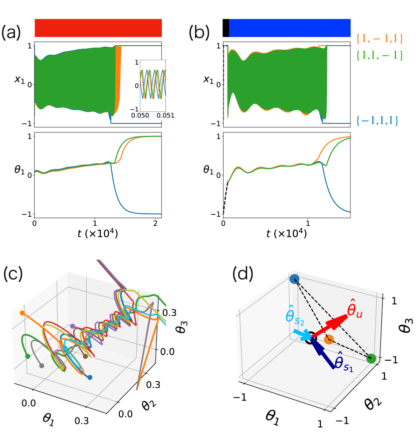
Figure 1: (a) Cell differentiation and (b) reprogramming of the repressilator model with $\tau=10^{3}$. Upper bar indicates differentiation (red), reprogramming manipulation (black), and later process (blue) without it ($I_{i}=0$). We plotted the time development of $x_{1},\theta_{1}$ (see Fig. S5abNote (2) for the time series of all variables). (a) Three trajectories are sampled from slightly different initial conditions near $\theta_{i}=0$. (b) From the fixed point $\{-1,1,1\}$, we tested three slightly different time spans to add external input (520, 530, 540). After reprogramming manipulation, the cellular state first approached $\theta_{1}=\theta_{2}=\theta_{3}$, and then differentiated to three fixed points again. (c) Trajectories through reprogramming and differentiation plotted in the $(\theta_{1},\theta_{2},\theta_{3})$ space. Ten attempts were overlaid by considering the initial conditions in $x_{i}\in[-1,1],\theta_{i}\in[-0.25,0.25]$, which allowed oscillation. Attraction for the straight line $\theta_{1}=\theta_{2}=\theta_{3}$ and departure from it was discernible. (d) Eigenvector $\{\bm{v}_{k}\}$ and variables $\{\hat{\theta}_{k}\}$ (see text). Three colored points represent the fixed points $\{-1,1,1\}$ (blue), $\{1,-1,1\}$ (orange), and $\{1,1,-1\}$ (green).

Next, we studied how the attraction to the straight line first occurs, followed by differentiation progression. For it, we considered the adiabatic limit of $\tau\rightarrow\infty$. For fixed $\theta_{i}$, we first obtained the attractor $x_{i}$. Then, the evolution of $\theta_{i}$ was obtained by replacing $x_{i}$ in Eq. (1b) by its time average $\bar{x}_{i}$ for a given $\theta_{i}$, as follows:

$$\frac{d\theta_{i}}{dt}=\bar{x}_{i}(\theta_{i})-\theta_{i}(\equiv\Theta_{i}).$$ (2)

In the three-variable Eq. (2), $\{\theta_{1},\theta_{2},\theta_{3}\}=\{0,0,0\}$ is a fixed point solution because $x_{i}(t)$ showed a symmetric limit-cycle oscillation, such that $\bar{x}_{i}=0$ for all $i$ therein for $\{\theta_{1},\theta_{2},\theta_{3}\}=\{0,0,0\}$. By slightly perturbing $\theta_{i}$ as a parameter, $\bar{x}_{j}$ changed accordingly. From $\partial\bar{x}_{i}/\partial\theta_{j}$, we obtained the Jacobi matrix $\partial\Theta_{i}/\partial\theta_{j}$ with eigenvalues $\{\lambda_{k}\}$ and eigenvectors $\{\bm{v}_{k}\}$. As shown in Fig. 1d, $\{\theta_{1},\theta_{2},\theta_{3}\}=\{0,0,0\}$-fixed point was a saddle, with the eigenvector $\bm{v}_{u}=\{1,1,1\}/\sqrt{3}$ corresponding to $\lambda_{u}>0$ (unstable axis), and $\bm{v}_{s_{1}}=\{2,-1,-1\}/\sqrt{6},\bm{v}_{s_{2}}=\{0,-1,1\}/\sqrt{2}$ for $\mathrm{Re}(\lambda_{s_{1}})=\mathrm{Re}(\lambda_{s_{2}})<0$ (see Supplemental Information (SI) 1ANote (2)). To investigate $\theta$ dynamics along each eigenvectors $\bm{v}_{k}$ ($k=u,s_{1},s_{2}$), we then introduced the variable $\hat{\theta}_{k}$, projection of $\bm{\theta}$ on $\bm{v}_{k}$ (that is, $\hat{\theta}_{k}=\bm{\theta}\cdot\bm{v}_{k}$, with $\bm{v}_{k}$ normalized). Noteworthy, owing to the symmetry of the repressilator, the unstable manifold was in line with the eigenvector $\bm{v}_{u}$ (see SI 1ANote (2)).

As shown in Fig. 1cd, the straight line to which all trajectories converged agreed with the unstable manifold $\bm{v}_{u}$ (Fig. 2a). Of course, attraction to the $\bm{v}_{u}$ axis was natural if the initial conditions were restricted to the stable manifold for $\{\theta_{1},\theta_{2},\theta_{3}\}=\{0,0,0\}$. However, we observed an attraction toward the unstable axis over a wide range of initial conditions for $\{\theta_{i}\}$, which supports the oscillation of $x_{i}$. Furthermore, the magnitudes of the eigenvalues for the stable and unstable eigenvectors were of the same order ($\mathrm{Re}(\lambda_{u})=0.31,\mathrm{Re}(\lambda_{s_{1}})=\mathrm{Re}(\lambda_{s_{2}})=-0.66$, see Fig. S5cNote (2)). Thus, the reprogramming dynamics shown in Fig. 1b could not be explained just by the linear stability.

To elucidate whether the nonlinear effect suppresses the instability along the $\bm{v}_{u}$ axis, we computed $d\hat{\theta}_{u}/dt$. As shown in Fig. 2c, $d\hat{\theta}_{u}/dt$ was drastically reduced from the linear case. We also computed $(d\hat{\theta}_{s_{1}}/dt,d\hat{\theta}_{s_{2}}/dt)$ for a certain $\hat{\theta}_{u}$ value (that is, the flow structure in the $(\hat{\theta}_{s_{1}},\hat{\theta}_{s_{2}})$ plane, sliced along the $\hat{\theta}_{u}$ axis), which showed that $\hat{\theta}_{s_{1}}=0$ changed from stable to unstable at $\hat{\theta}_{u}=\hat{\theta}_{u}^{\mathrm{th}}(\sim 0.4)$ (see Fig. 2d and Fig. S6Note (2)). Up to $\hat{\theta}_{u}<\hat{\theta}_{u}^{\mathrm{th}}(\sim 0.4)$, $\theta_{i}$ in $(\hat{\theta}_{s_{1}},\hat{\theta}_{s_{2}})$ plane was attracted to the $\hat{\theta}_{u}$ axis. By further increasing $\hat{\theta}_{u}$ beyond $\hat{\theta}_{u}^{\mathrm{th}}$, $\theta_{i}$ departured from the $\hat{\theta}_{u}$ axis rotating in the $(\hat{\theta}_{s_{1}},\hat{\theta}_{s_{2}})$ plane, leading to differentiation into three distinct fixed points.

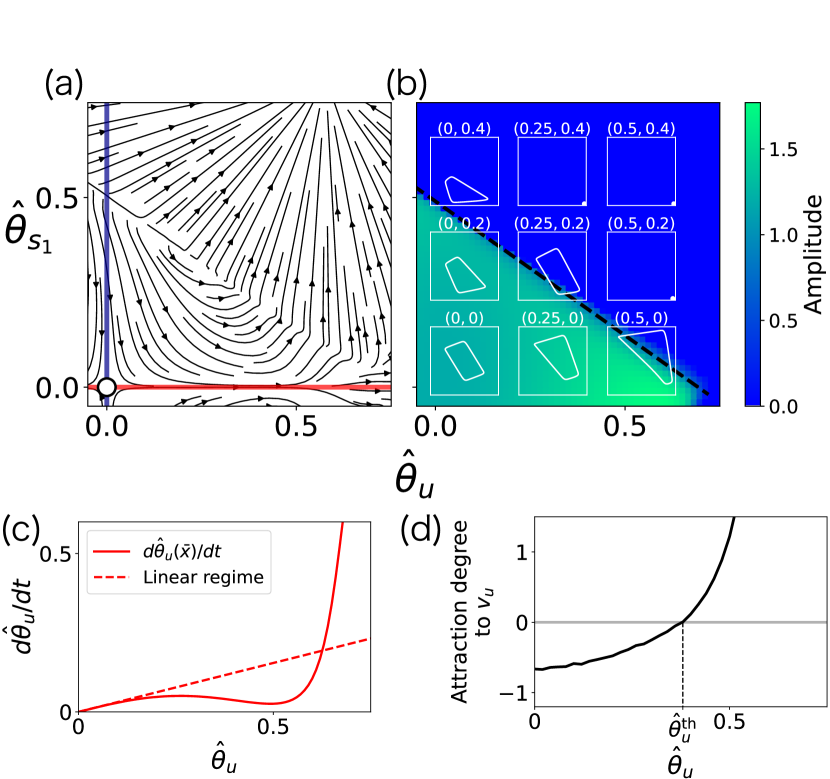
Figure 2: (a) Stream plot of $(d\hat{\theta}_{u}/dt,d\hat{\theta}_{s_{1}}/dt)$ in $(\hat{\theta}_{u},\hat{\theta}_{s_{1}})$ space according to Eq. (2). Red (blue) line represents the direction of the eigenvector $\bm{v}_{u}(\bm{v}_{s_{1}})$. (b) Attractors in the $x$-space for each fixed $\theta$ value. For the green (blue)-colored region, the attractor in the $x$ space was the limit cycle (fixed point). Each trajectory shows the dynamics in the $x_{1}-x_{2}$ space for $(\hat{\theta}_{u},\hat{\theta}_{s_{1}})$ (both $x_{1}$ and $x_{2}$ axes for all figures are ranged within $\{-1.05,1.05\}$). (c) $d\hat{\theta}_{u}/dt$ plotted as a function of $\hat{\theta}_{u}$. For comparison, we plotted $d\hat{\theta}_{u}=\lambda_{u}\hat{\theta}_{u}$(red dotted line). (d) Degree of attraction to $\bm{v}_{u}$. $\nu$, in the text, is plotted as a function of $\hat{\theta}_{u}$. If it is negative (positive), $\{\theta\}$ was attracted to (departed from) $\bm{v}_{u}$. See Fig. S6Note (2) for more detail.

To unveil how the slow motion along $\hat{\theta}_{u}$ and the attraction to $\hat{\theta}_{u}$ occurred, we first fixed $\theta_{i}$ and studied the change in the $x$ attractor, as shown in Fig. 2b. In the green (blue) region, the $x$ attractor was a limit cycle (fixed point) for $(\hat{\theta}_{u},\hat{\theta}_{s_{1}})$. At the line $\hat{\theta}_{s_{1}}=-\hat{\theta}_{u}/\sqrt{2}+\sqrt{6}/5$ (as discussed in SI 1BCNote (2)), $x$-dynamics exhibited bifurcation from the limit cycle to a fixed point $\{1,-1,1\}$ (see Fig. S7Note (2) for more details). Considering the symmetry of the repressilator, bifurcations to three fixed points $\{-1,1,1\},\{1,-1,1\},\{1,1,-1\}$ coexisted in the $(\hat{\theta}_{s_{1}},\hat{\theta}_{s_{2}})$ plane. With the increase of $\hat{\theta}_{u}$, the limit cycle approached the three fixed points.

Now, we discussed the mechanism of slow motion along $\hat{\theta}_{u}$. From Eq. (2), movement along $\bm{v}_{u}$ followed $d\hat{\theta}_{u}/dt=\bar{x}_{u}(\hat{\theta}_{u})-\hat{\theta}_{u}$ (we defined $x_{k}$ as a projection on $\bm{v}_{k}$). As shown in Fig. 3a, the limit cycle approached the plane spanned by the three fixed points $\{-1,1,1\},\{1,-1,1\},\{1,1,-1\}$ as $\hat{\theta}_{u}$ increased. In the plane, $\bar{x}_{u}$ comprised $1/\sqrt{3}$, and $\theta_{i}$ increased following Eq. (2) (see SI 1DNote (2) for more details). Then, as $\hat{\theta}_{u}$ approaches $1/\sqrt{3}$, $d\hat{\theta}_{u}/dt$ was minimized, as shown in Fig. 2c.

Next, we considered how attraction to the $\bm{v}_{u}$ from the $(\hat{\theta}_{s_{1}},\hat{\theta}_{s_{2}})$ plane was lost at the $\hat{\theta}_{u}=\hat{\theta}_{u}^{th}$. By considering $\hat{\theta}_{u}$ as a parameter, the direction of flow in the $(\hat{\theta}_{s_{1}},\hat{\theta}_{s_{2}})$ plane toward the $\bm{v}_{u}$ was determined by the sign of $\partial\Theta_{s_{1}}/\partial\hat{\theta}_{s_{1}}=\partial\bar{x}_{s_{1}}/\partial\hat{\theta}_{s_{1}}-1\equiv\nu\Theta_{s_{1}}$ (we defined $\Theta_{s_{1}}$ as a projection on $\bm{v}_{s_{1}}$). As shown in Fig 2b, with the increase in $\hat{\theta}_{u}$, the bifurcation point from the limit cycle to the fixed point approached the $\hat{\theta}_{u}=0$ line. Hence, by slightly changing $\hat{\theta}_{s_{1}}$, $\bar{x}$ reached fixed points. Accordingly, $\partial\bar{x}_{s_{1}}/\partial\hat{\theta}_{s_{1}}$ increase beyond one, so that $\partial\Theta_{s_{1}}/\partial\hat{\theta}_{s_{1}}$ became positive at $\hat{\theta}_{u}$, approaching $\hat{\theta}_{u}^{\mathrm{th}}\sim 0.4$, as shown in Figs. 2d and 3b.

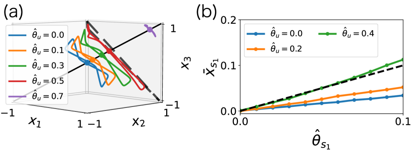
Figure 3: (a) Change in the limit cycle $x(t)$ (closed line) and $\bar{x}$ (point) along $\hat{\theta}_{u}$. Black dotted line shows an equilateral triangle with corners $\{-1,1,1\},\{1,-1,1\},\{1,1,-1\}$ (see SI 1DNote (2)). (b) $\bar{x}_{s_{1}}$ as a function of $\hat{\theta}_{s_{1}}$. The slope of each line corresponds to $\partial\bar{x}_{s_{1}}/\partial\hat{\theta}_{s_{1}}$ for $\hat{\theta}_{u}$. From $\partial\Theta_{s_{1}}/d\hat{\theta}_{s_{1}}$, if the slope is less than one, the orbits are attracted toward $\hat{\theta}_{u}$. For comparison, we plotted $\bar{x}_{s_{1}}=\hat{\theta}_{s_{1}}$ as a black dotted line. At $\hat{\theta}_{u}\sim 0.4$, $\partial\bar{x}_{s_{1}}/\partial\hat{\theta}_{s_{1}}$ exceeds one.

Thus, we have unveiled how attraction to the unstable manifold is achieved by slow epigenetic fixation of the oscillation of fast gene expression in the repressilator model. Following this picture, reprogramming is possible by forcing the cells to return to the oscillatory state. Then, the cell is attracted to a pluripotent state with low epigenetic modification $\theta_{i}\sim 0$, from which differentiation to distinct cell types with specific $\theta$ values follows.

To verify the generality of this reprogramming scheme, we examined several GRN models with more degrees of freedom. As discussed in Matsushita and Kaneko (2020), differentiation from oscillatory states is often observed in GRNs (e.g., 20% of randomly generated GRNs show oscillatory dynamics for $N=10$). An example is shown in Fig. S8aNote (2). From a differentiated state, we overexpressed three genes to regain oscillatory expression (black line in Fig. S8aNote (2)). Later, global attraction to unstable manifold also occurred as discussed above. Then, the cell states branch to distinct fixed point states again (blue line in Fig. S8aNote (2)). In these cases, the original pluripotent state with $\theta=0$ was an unstable fixed point, with one positive eigenvalue for the Jacobi matrix of $\theta$ dynamics (Fig. S8dNote (2)), as in the repressilator model. Even though the degrees of freedom increased, the unstable manifold is one-dimensional, and the attraction to the manifold occurred from a higher-dimensional state space. This implies that reprogramming manipulation requires only partial degrees of freedom compared with the total number of genes. In fact, overexpression of three genes is sufficient for reprogramming in GRN models with $N=10$, as far as we have investigated.

The present mechanism also works in a model extracted from GRN for an ES cell Dunn et al. (2014), as a core network with five genes (Nanog, Oct4, Gata6, Gata4, and Klf4) Miyamoto et al. (2015) (see Fig. S4b). Oct4, Sox2, and Klf4 are known as factors to induce reprogramming. The model involves a negative feedback loop, as in the repressilator, in addition to positive feedback regulation. In this five-gene model, $x_{i}$ and $\theta_{i}$ oscillate in the region near the origin, and then differentiation to three fixed points progresses as in the repressilator case (three lines in Fig. 4a), whereas $\theta_{i}=0$ for all $i$ represents a saddle point with one unstable manifold and four stable manifolds, as shown in Fig.S9b. After overexpression of Oct4, Nanog, and Klf4 in one of the differentiated cell types for a certain time span (black dotted line in Fig. 4b), the epigenetic state $\theta_{i}$ approached the unstable manifold for the unstable fixed point $\theta_{i}=0$, leading to recovery of pluripotency (blue line in Fig. 4b).

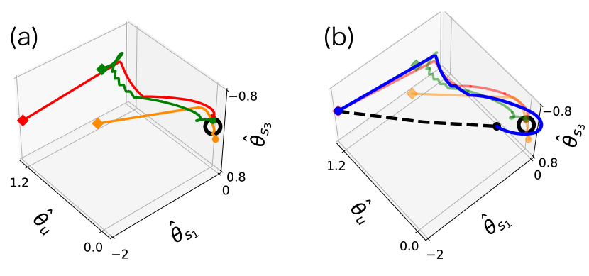
Figure 4: (a) Cell differentiation and (b) reprogramming in the five-gene model (a) Three orbits starting from the vicinity of the saddle point $\theta_{i}=0$ for all $i$ (black dotted point), reached three distinct cell types. (b) From differentiated cell types (red point), we added external input $I_{i}(t)$ to Nanog, Oct4, and Klf4 for a certain time span (black dotted line). After such reprogramming manipulation, we set $I_{i}(t)=0$. The cell state then spontaneously approached the saddle point, and the reinitiated the differentiation progression again (blue line). $\tau=10^{3}$. See Fig. S9Note (2) for more detail.

In this letter, we have shown that oscillatory gene expression dynamics with slow epigenetic modifications lead to cellular reprogramming by overexpression of only few genes. The global attraction to the unstable manifold of the saddle point explains the reprogramming process. Now, the return to the top of the landscape by reprogramming, which is seemingly unstable, is explained by the strong attraction toward the unstable manifold of the saddle, and suppressed instability along with the unstable manifold, owing to the approach of limit-cycle of bifurcation to fixed points. The memory of the cellular state before reprogramming manipulation was erased through this reprogramming process.

Moreover, regain of oscillation was found to be the main requirement for reprogramming, whereas elaborate manipulations to induce a cellular state into specific states is not necessary. This explains the role of oscillations in gene expression in pluripotent cells Kobayashi et al. (2009) and epigenetic modification through the differentiation process Rulands et al. (2018), as well as it explains how reprogramming is possible by overexpressing just few genes among thousand of that Takahashi and Yamanaka (2006); Velychko et al. (2019). The timescale separation between fast expression dynamics and slow epigenetic modification feedback required is also consistent with previous observations Barth and Imhof (2010); Maeshima et al. (2015). In future studies, experimental support is necessary, as well as theoretical analysis of slow-fast dynamical systems Aoki and Kaneko (2013); Kuehn (2015).