Implicit Copulas: An Overview

Abstract

Implicit copulas are the most common copula choice for modeling dependence in high dimensions. This broad class of copulas is introduced and surveyed, including elliptical copulas, skew $t$ copulas, factor copulas, time series copulas and regression copulas. The common auxiliary representation of implicit copulas is outlined, and how this makes them both scalable and tractable for statistical modeling. Issues such as parameter identification, extended likelihoods for discrete or mixed data, parsimony in high dimensions, and simulation from the copula model are considered. Bayesian approaches to estimate the copula parameters, and predict from an implicit copula model, are outlined. Particular attention is given to implicit copula processes constructed from time series and regression models, which is at the forefront of current research. Two econometric applications—one from macroeconomic time series and the other from financial asset pricing—illustrate the advantages of implicit copula models.

[1]organization=Melbourne Business School, University of Melbourne, addressline=200 Leicester Street, city=Carlton, postcode=3053, country=Australia

1 Introduction

Copulas are widely used to specify multivariate distributions for the statistical modeling of data. Fields where copula models have had a significant impact include (but are not limited to) actuarial science (Frees and Valdez, 1998), finance (Cherubini et al., 2004; McNeil et al., 2005; Patton, 2006), hydrology (Favre et al., 2004; Genest et al., 2007), climatology (Schoelzel and Friederichs, 2008), transportation (Bhat and Eluru, 2009; Smith and Kauermann, 2011) and marketing (Danaher and Smith, 2011; Park and Gupta, 2012). Copula models are popular because they simplify the specification of a distribution, allowing the marginals to be modeled arbitrarily, and then combined using a copula function. In practice, a major challenge is the selection and estimation of a copula function that captures the dependence structure well and is tractable. One choice are “implicit copulas”, which are copulas constructed from existing multivariate distributions by the inversion of Sklar’s theorem as in Nelsen (2006, p.51). This is a large and flexible family of copulas, which share an auxiliary representation that makes estimation tractable in high dimensions. Thus, they are suitable for modeling the large datasets that arise in many modern applications. The objective of this paper is to introduce and survey implicit copulas and their use in statistical modeling in an accessible manner.

Implicit copulas have a long history with key developments spread across multiple fields, including actuarial studies, econometrics, operations research, probability and statistics. Yet while there are many excellent existing monographs and surveys on copulas and copula models (see Genest and MacKay (1986); Joe (1997); McNeil et al. (2005); Nelsen (2006); Genest and Nešlehová (2007); Jaworski et al. (2010); Patton (2012); Nikoloulopoulos (2013a); Joe (2014) and Durante and Sempi (2015) for prominent examples) there does not appear to be a dedicated survey or overview on this important class of copulas. This paper aims to fill this gap and provides an overview that stresses common features of the implicit copula family, likelihood-based estimation, and the usefulness of implicit copulas in statistical modeling. Particular focus is given to recent developments on implicit copula processes for regression and time series data, along with Bayesian inference that extends the earlier overview by Smith (2013) to these copula processes.

Two econometric applications illustrate the use of implicit copula models with non-Gaussian data. The first is a time-varying heteroscedastic time series model for U.S. inflation between 1954:Q1 and 2020:Q2. The implicit copula is a copula process constructed from a nonlinear state space model as in Smith and Maneesoonthorn (2018). It is a “time series copula” that captures serial dependence. The second application is a five factor asset pricing regression model (Fama and French, 2015) with an asymmetric Laplace marginal distribution for monthly equity returns. The implicit copula here is a “regression copula” process with respect to the covariates as in Klein and Smith (2019). The copula model forms a distributional regression (Klein et al., 2015; Kneib et al., 2021), where the five factors affect the entire distribution of equity returns, not just its first or other moments. In both applications the implicit copulas are of dimension equal to the number of observations, so that they are high-dimensional. Nevertheless, their auxiliary representation allows for likelihood-based estimation of the copula parameters. In both examples the marginal distribution of the response variables exhibit strong asymmetries.

The overview is organized as follows. Section 2 introduces general copula models, and then implicit copulas specifically. Their interpretation as transformations and specifications for variables that are continuous, discrete or mixed are also discussed. Section 3 covers elliptical and skew-elliptical copulas, including the Gaussian, $t$, skew $t$ and factor copulas. Implicit copulas that capture serial dependence in time series data are covered in Section 4. Section 5 extends these to implicit copulas that capture both serial and cross-sectional dependence in multivariate time series. Section 6 covers regression copula processes, with the implicit copula constructed from a regularized linear regression given in detail. It is shown that when this copula is combined with flexible marginals, it defines a promising new distributional regression model. Last, Section 7 discusses the advantages of using implicit copula models for modeling data, and future directions.

2 Implicit copulas

2.1 Copula models in general

All copula models are based on the theorem of Sklar (1959) (i.e. “Sklar’s theorem”), which states that for every random vector $\bm{Y}=(Y_{1},\ldots,Y_{m})^{\top}$ with distribution function $F_{Y}$ and marginals $F_{Y_{1}},\ldots,F_{Y_{m}}$, there exists a “copula function” $C:[0,1]^{m}\rightarrow[0,1]$, such that

$$F_{Y}(\bm{y})=C(F_{Y_{1}}(y_{1}),\ldots,F_{Y_{m}}(y_{m}))\,,$$ (1)

where $\bm{y}=(y_{1},\ldots,y_{m})^{\top}$. The copula function $C$ is a well-defined distribution function for a random vector $\bm{U}=(U_{1},\ldots,U_{m})^{\top}$ on the unit cube with uniform marginal distributions. To construct a copula model, select $F_{Y_{1}},\ldots,F_{Y_{m}}$ (i.e. the “marginal models”) and a copula function $C$, to define $F_{Y}$ via (1).

2.1.1 Continuous case

If all the elements of $\bm{Y}$ are continuous, then differentiating through (1) gives the density

$$f_{Y}(\bm{y})=\frac{\partial^{m}}{\partial y_{1}\cdots\partial y_{m}}F_{Y}(\text{\boldmath$y$})=c(F_{Y_{1}}(y_{1}),\ldots,F_{Y_{m}}(y_{m}))\prod_{j=1}^{m}f_{Y_{j}}(y_{j})\,,$$ (2)

where $f_{Y_{j}}=\frac{\partial}{\partial y_{j}}F_{Y_{j}}$, and $c(\bm{u})=\frac{\partial^{m}}{\partial u_{1}\cdots\partial u_{m}}C(\bm{u})$ is widely called the “copula density” with $\bm{u}=(u_{1},\ldots,u_{m})^{\top}$. (Throughout this paper the notation $c(\text{\boldmath$u$})$ and $c(u_{1},u_{2},\ldots,u_{m})$ are used interchangeably, as are $C(\text{\boldmath$u$})$ and $C(u_{1},u_{2},\ldots,u_{m})$.) The decomposition at (2) is used to specify the likelihood of a continuous response vector $\bm{Y}$ in a statistical model.

2.1.2 Discrete case

If all the elements of $\bm{Y}$ are discrete-valued (e.g. as with ordinal or binary data) the probability mass function is obtained by differencing over the elements of $\bm{Y}$ as follows. Let $b_{j}=F_{Y_{j}}(y_{j})$ and $a_{j}=F_{Y_{j}}(y_{j}^{-})$ be the left-hand limit of $F_{j}$ at $y_{j}$ (which is $a_{j}=F_{Y_{j}}(y_{j}-1)$ for ordinal $Y_{j}$). Then the mass function is

$$f_{Y}(\bm{y})=\mbox{Pr}(Y_{1}=y_{1},\ldots,Y_{m}=y_{m})=\Delta_{a_{1}}^{b_{1}}\Delta_{a_{2}}^{b_{2}}\cdots\Delta_{a_{m}}^{b_{m}}C(\text{\boldmath$v$})\,,$$ (3)

where $\text{\boldmath$v$}=(v_{1},\ldots,v_{m})^{\top}$ is a differencing vector, and the notation

$$\Delta_{a_{j}}^{b_{j}}C(u_{1},\ldots,u_{j-1},v_{j},u_{j+1},\ldots,u_{m})$$

$$= C(u_{1},\ldots,u_{j-1},b_{j},u_{j+1},\ldots,u_{m})-C(u_{1},\ldots,u_{j-1},a_{j},u_{j+1},\ldots,u_{m})\,.$$

Evaluating the mass function at (3) is an $O(2^{m})$ computation, so that its direct evaluation is impractical for high values of $m$ when undertaking likelihood-based estimation (Nikoloulopoulos, 2013a). One solution suggested by Smith and Khaled (2012) is to consider the joint distribution of $(\bm{Y},\bm{U})$. To do so, note that when $Y_{j}$ is discrete, $F_{Y_{j}}$ is a many-to-one function and $Y_{j}|U_{j}$ is a degenerate distribution with density $f(y_{j}|u_{j})=\mathds{1}(a_{j}\leq u_{j}<b_{j})$, where the indicator function $\mathds{1}(X)=1$ if $X$ is true, and zero otherwise. (An alternative notation is to use the Dirac delta function, with $f(y_{j}|u_{j})=\delta_{y_{j}}(F_{Y_{j}}^{-}(u_{j}))$ where $F_{Y_{j}}^{-}$ is the quantile function of $Y_{j}$.) Then the mixed density of $(\bm{Y},\bm{U})$ is

$$f_{Y,U}(\text{\boldmath$y$},\text{\boldmath$u$})=f(\text{\boldmath$y$}|\text{\boldmath$u$})c(\text{\boldmath$u$})=\prod_{j=1}^{m}\left\{\mathds{1}(a_{j}\leq u_{j}<b_{j})\right\}c(\text{\boldmath$u$})\,.$$ (4)

Marginalizing over $\bm{U}$ gives the probability mass function at (3) (i.e. $f_{Y}(\text{\boldmath$y$})=\int f_{Y,U}(\text{\boldmath$y$},\text{\boldmath$u$})\mbox{d}\text{\boldmath$u$}$); see Proposition 1 in Smith and Khaled (2012).

Equation (4) can be used to define an “extended likelihood” for estimation using computational methods for latent variables, where the observations on $\bm{U}$ are the latents. This has two advantages. First, the $O(2^{m})$ computation at (3) is avoided, allowing estimation for higher values of $m$. Second, only the copula density $c$ is required and not the copula function $C$, which is an advantage for some copulas where only $c$ can be computed, as is the case with most vine copulas (Joe, 1996; Aas et al., 2009). Bayesian data augmentation can be used based on (4), and evaluated using Markov chain Monte Carlo (MCMC) as in Smith and Khaled (2012) or variational Bayes methods as in Loaiza-Maya and Smith (2019). The latter is particularly attractive, because it allows for the estimation of discrete-margined copulas of very high dimensions, with examples up to $m=792$ presented by these authors.

2.1.3 Mixed cases

If some elements of $\bm{Y}$ are continuous and others discrete, then $f_{Y}$ is often called a “mixed density”. In this case, an extended likelihood can be constructed from the distribution of $\bm{Y}$ joint with the elements of $\bm{U}$ that correspond only to the discrete variables; see Smith and Khaled (2012, Sec.6). Similarly, if some individual elements $Y_{j}$ have distributions that are mixtures of continuous and discrete distributions (such as a zero-inflated continuous distribution) then an extended likelihood can also be constructed for this case; see Gunawan et al. (2020) for how to do so.

2.2 The basic idea of an implicit copula

McNeil et al. (2005, p.190) use the term “implicit copula” for the copula that is implicit in the multivariate distribution of a continuous random vector $\bm{Z}=(Z_{1},\ldots,Z_{m})^{\top}$. It is obtained by inverting Sklar’s theorem, which Nelsen (2006, p.51) calls the “inversion method”, so that copulas derived in this fashion are also called “inversion copulas” (e.g. Smith and Maneesoonthorn (2018)). If $\bm{Z}$ has distribution function $F_{Z}$ with marginals $F_{Z_{1}},\ldots,F_{Z_{m}}$, then its implicit copula function is

$$C_{Z}(\text{\boldmath$u$})=F_{Z}\left(F_{Z_{1}}^{-1}(u_{1}),\ldots,F_{Z_{m}}^{-1}(u_{m})\right)\,.$$ (5)

Differentiating with respect to $u$ gives the implicit copula density

$$c_{Z}(\text{\boldmath$u$})=\frac{\partial^{m}}{\partial u_{1}\cdots\partial u_{m}}C(\text{\boldmath$u$})=\frac{f_{Z}(\text{\boldmath$z$})}{\prod_{j=1}^{m}f_{Z_{j}}(z_{j})}\,,$$ (6)

where $\text{\boldmath$z$}=(z_{1},\ldots,z_{m})^{\top}$ is a function of $u$ with elements $z_{j}=F_{Z_{j}}^{-1}(u_{j})$ for $j=1,\ldots,m$. The implicit copula function $C_{Z}$ and density $c_{Z}$ above can be employed in (1), (2) and (3). Thus, an implicit copula model uses Sklar’s theorem twice: once to form the joint distribution $F_{Y}$ with arbitrary marginals, and a second time to construct the implicit copula from the joint distribution $F_{Z}$.

Because implicit copulas are an immediate consequence of Sklar’s theorem, they have a long history. Early uses for modelling data include Rüschendorf (1976) and Deheuvels (1979), who both construct a non-parametric implicit copula from the empirical distribution function (although neither called it a copula). Rüschendorf (2009) gives an overview of the early developments of implicit copulas, pointing out that many transformation-based multivariate models—which themselves have a long history—are also copula models based on implicit copulas (although in the early literature this was often unrecognized and the term “copula” not used).

Note that only a continuous distribution $F_{Z}$ is used to construct an implicit copula here. This is because the implicit copula of a discrete distribution $F_{Z}$ is not unique (Genest and Nešlehová, 2007).

2.3 Implicit copulas as transformations

One way to look at all copula models is that they are a transformation from $\bm{Y}$ to $\bm{U}=(U_{1},\ldots,U_{m})^{\top}\in[0,1]^{m}$. The key observation is that it is usually easier to capture multivariate dependence using $C$ on the vector space $[0,1]^{m}$, rather than directly on the domain of the original vector $\bm{Y}$. Implicit copulas go one step further, with a second transformation from $\bm{U}$ to $\bm{Z}=(F_{Z_{1}}^{-1}(U_{1}),\ldots,F_{Z_{m}}^{-1}(U_{m}))^{\top}$, and then capture the dependence structure using the distribution $F_{Z}$. Table 1 provides a summary of these transformations, along with the marginal and joint distribution and density/mass functions of $\bm{Y}$. Throughout this paper, the vector $\bm{U}$ is referred to as the “copula vector” and $\bm{Z}$ as the “auxiliary vector” (the latter is also called a “pseudo vector” in Smith and Klein (2021)). Simulation from an implicit copula model is straightforward if $F_{Z}$ is tractable using Algorithm 1, which produces a draw $\text{\boldmath$y$}\sim F_{Y}$.

Algorithm 1 (Random iterate generation from an implicit copula model)

• Generate $\text{\boldmath$z$}=(z_{1},\ldots,z_{m})^{\top}\sim F_{Z}$

• For $j=1,\ldots,m$, set $u_{j}=F_{Z_{j}}(z_{j})$, and $\text{\boldmath$u$}=(u_{1},\ldots,u_{m})^{\top}$

• For $j=1,\ldots,m$, set $y_{j}=F_{Y_{j}}^{-1}(u_{j})$, and $\text{\boldmath$y$}=(y_{1},\ldots,y_{m})^{\top}$

Notice that the transformation $U_{j}=F_{Z_{j}}(Z_{j})\sim\mbox{Uniform}[0,1]$ removes all features of the marginal distribution of $Z_{j}$. This becomes an important observation for establishing parameter identification when constructing implicit copulas, as discussed in Sections 4, 5 and 6.

Table 1: Transformational relationships between observational vector $\bm{Y}$, copula vector $\bm{U}$ and auxiliary vector $\bm{Z}$ for an implicit copula

	Observational	Copula	Auxiliary
Random Variable	Continuous $Y_{j}$	$U_{j}=F_{Y_{j}}(Y_{j})$	$Z_{j}=F_{Z_{j}}^{-1}(U_{j})$
	Discrete $Y_{j}$	$F_{Y_{j}}(Y_{j}^{-})\leq U_{j}<F_{Y_{j}}(Y_{j})$	$F_{Z_{j}}^{-1}(F_{Y_{j}}(Y_{j}^{-}))\leq Z_{j}<F_{Z_{j}}^{-1}(F_{Y_{j}}(Y_{j}))$
Domain	${\cal D}_{Y_{1}}\times\cdots\times{\cal D}_{Y_{m}}$	$[0,1]^{m}$	${\cal D}_{Z_{1}}\times\cdots\times{\cal D}_{Z_{m}}$
Marginal Distribution	$F_{Y_{j}}$	Uniform	$F_{Z_{j}}$
Joint Distribution	$F_{Y}(\text{\boldmath$y$})=C(\text{\boldmath$u$})$	$C(\text{\boldmath$u$})=F_{Z}(F_{Z_{1}}^{-1}(u_{1}),\ldots,F_{Z_{m}}^{-1}(u_{m}))$	$F_{Z}$
Joint Density/Mass
($Y_{j}$ Continuous)	$f_{Y}(\bm{y})=c(\text{\boldmath$u$})\prod_{j=1}^{m}f_{Y_{j}}(y_{j})$	$c(\bm{u})=\frac{f_{Z}(\text{\boldmath$z$})}{\prod_{j=1}^{m}f_{Z_{j}}(z_{j})}$	$f_{Z}(\text{\boldmath$z$})$
($Y_{j}$ Discrete)	$f_{Y}(\bm{y})=\Delta_{a_{1}}^{b_{1}}\Delta_{a_{2}}^{b_{2}}\cdots\Delta_{a_{m}}^{b_{m}}C(\text{\boldmath$v$})$

The joint distribution and density/mass functions of $\bm{Y}=(Y_{1},\ldots,Y_{m})^{\top}$, $\bm{U}=(U_{1},\ldots,U_{m})^{\top}$ and $\bm{Z}=(Z_{1},\ldots,Z_{m})^{\top}$ are given. The joint density of $\bm{Y}$ is given separately when all the elements are continuous and when all the elements are discrete. When some elements are discrete and others continuous, the mixed density is given in Smith and Khaled (2012, Sec.6). In this table, ${\cal D}_{Y_{j}}$ is the domain of $Y_{j}$, and ${\cal D}_{Z_{j}}$ is the domain of $Z_{j}$.

2.4 An alternative extended likelihood

For the case where the elements of $\bm{Y}$ are discrete-valued, for an implicit copula model there exists an alternative extended likelihood based on the joint density of $(\bm{Y},\bm{Z})$, rather than that of $(\bm{Y},\bm{U})$ given previously at (4). This alternative joint density is

$$f_{Y,Z}(\text{\boldmath$y$},\text{\boldmath$z$})=f(\text{\boldmath$y$}|\text{\boldmath$z$})f_{Z}(\text{\boldmath$z$})=\prod_{j=1}^{m}\left\{\mathds{1}\left(F_{Z_{j}}^{-1}(a_{j})\leq z_{j}<F_{Z_{j}}^{-1}(b_{j})\right)\right\}f_{Z}(\text{\boldmath$z$})\,,$$ (7)

with $a_{j},b_{j}$ as defined above in Section 2.1.2. Marginalizing over $\bm{Z}$ produces the probability mass function at (3); i.e. $f_{Y}(\text{\boldmath$y$})=\int f_{Y,Z}(\text{\boldmath$y$},\text{\boldmath$z$})\mbox{d}\text{\boldmath$z$}$. An advantage is that it is often simpler to use computational methods to estimate an implicit copula using (7) rather than (4). Moreover, an extended likelihood is also easily defined for vectors $\bm{Y}$ with combinations of discrete, continuous or even mixed valued elements, by simplifying (7) to only include elements of $\bm{Z}$ that correspond to the non-continuous valued variables.

Bayesian data augmentation is a suitable method for estimation using this extended likelihood. Here, values for $z$ are generated in an MCMC sampling scheme to evaluate an “augmented posterior” proportional to the extended likelihood multiplied by a parameter prior. This has been used to estimate the elliptical and skew elliptical copulas discussed in Section 3 below. For example, Pitt et al. (2006) do so for a Gaussian copula, while Danaher and Smith (2011) do so for the $t$ copula, and Smith et al. (2012) for the skew $t$ copula. Hoff et al. (2007) considered the extended likelihood above using empirical marginals and rank data, Danaher and Smith (2011) and Dobra et al. (2011) provide early applications to higher dimensional Gaussian $F_{Z}$. Last, the multivariate probit model is a Gaussian copula model, and the popular approach of Chib and Greenberg (1998) is a special case of these data augmentation algorithms.

3 Elliptical and Skew Elliptical Copulas

In practice, parametric copulas $C(\text{\boldmath$u$};\text{\boldmath$\theta$})$ with parameter vector $\theta$ are almost always used in statistical modelling, with McNeil et al. (2005), Nelsen (2006) and Joe (2014) giving overviews of choices. However, the implicit copulas of elliptical distributions, and more recently skew elliptical distributions, are common choices for capturing dependence in many applications. An attractive feature is that because elliptical and skew elliptical distributions are closed under marginalization, so are their implicit copulas.

3.1 Elliptical copulas

3.1.1 Gaussian copula

The simplest and most popular elliptical copula is the “Gaussian copula”, which is constructed from $\bm{Z}\sim N_{m}(\bm{0},\Omega)$ with $\Omega$ an $m\times m$ correlation matrix. If $\Phi_{m}(\cdot;\text{\boldmath$a$},\Omega)$ denotes an $N_{m}(\text{\boldmath$a$},\Omega)$ distribution function, and $\Phi(\cdot)$ a $N(0,1)$ distribution function, then from (5) the Gaussian copula function is

$$C_{\tiny{\mbox{G}a}}(\text{\boldmath$u$};\Omega)=\Phi_{m}\left(\Phi^{-1}(u_{1}),\ldots,\Phi^{-1}(u_{m});\bm{0},\Omega\right)\,.$$

If $\phi_{m}(\cdot;\text{\boldmath$a$},\Omega)$ is a $N_{m}(\text{\boldmath$a$},\Omega)$ density, and $\phi$ is a standard normal density, then plugging the Gaussian densities into (6) gives the Gaussian copula density

$$c_{\tiny{\mbox{G}a}}(\text{\boldmath$u$};\Omega)=\phi_{m}(\text{\boldmath$z$};\bm{0},\Omega)/\prod_{j=1}^{m}\phi(z_{j})\\ =|\Omega|^{-1/2}\exp\left\{-\frac{1}{2}\text{\boldmath$z$}^{\top}(\Omega^{-1}-I_{m})\text{\boldmath$z$}\right\}\,,$$

with $\text{\boldmath$z$}=(\Phi^{-1}(u_{1}),\ldots,\Phi^{-1}(u_{m}))^{\top}$.

There are a number of immediate observations on the Gaussian copula. First, the auxiliary vector $\bm{Z}$ has a distribution with a zero mean and unit marginal variances. This is because information about the first two marginal moments of $Z_{j}$ are lost in the transformation $U_{j}=F_{Z_{j}}(Z_{j})$ and are unidentified in the copula density. Second, adopting any constant mean value (other than zero) and marginal variances (other than unit values) for $\bm{Z}$ produces the same Gaussian copula $C_{\tiny{\mbox{G}a}}$. Third, closure under marginalization means that if $\bm{U}$ has distribution function $C_{\tiny{\mbox{G}a}}(\text{\boldmath$u$};\Omega)$, then any subset $\bm{U}_{0}$ of elements of $\bm{U}$ has distribution function $C_{\tiny{\mbox{G}a}}(\text{\boldmath$u$}^{0};\Omega^{0})$, where $\Omega^{0}$ is a correlation matrix made up of the corresponding rows and columns of $\Omega$.

A fourth observation is that any parametric correlation structure for $\bm{Z}$ is inherited by the Gaussian copula. It is this property that has led the widespread adoption of Gaussian copula models for modeling time series (Cario and Nelson, 1996), longitudinal (Lambert and Vandenhende, 2002), cross-sectional (Murray et al., 2013) and spatial (Bai et al., 2014; Hughes, 2015) data. The Gaussian copula has a long history, particularly when formed implicitly via transformation (e.g. Li and Hammond (1975)), although some early and influential mentions include Joe (1993), Clemen and Reilly (1999) and Wang (1999), while Li (2000) popularized its use in finance. A comprehensive overview of the Gaussian copula and its properties is given by Song (2000).

3.1.2 Other elliptical copulas

Fang et al. (2002) and Embrechts et al. (2002) use an elliptical distribution for $\bm{Z}$, and study the resulting class of “elliptical copulas”. When combined with choices for the marginals of $\bm{Y}$ in a copula model, Fang et al. (2002) call the distribution $F_{Y}$ “meta-elliptical”, and an overview of their dependence properties is given by Abdous et al. (2005). After the Gaussian copula, the most popular elliptical copula is the $t$ copula, where a multivariate $t$ distribution with degrees of freedom $\nu>0$ is adopted for $\bm{Z}$. Embrechts et al. (2002) and Venter (2003) study this copula, and the main advantage is that it can capture higher dependence in extreme values, which is important for financial and actuarial variables. A lesser known property is that values of $\nu$ close to zero allow for positive dependence between squared elements of $\bm{Y}$. This is useful for capturing the serial dependence in heteroscedastic time series, such as equity returns in finance; see Loaiza-Maya et al. (2018) and Bladt and McNeil (2021).

3.2 Skew elliptical copulas

3.2.1 Overview

Elliptical copulas exhibit radial symmetry, where the distributions of $(U_{i},U_{j})$ and $(1-U_{i},1-U_{j})$ are the same. Yet there are applications where this is unrealistic, including for the dependence between equity returns (Longin and Solnik, 2001; Ang and Chen, 2002) and regional electricity spot prices (Smith et al., 2012). The implicit copulas of skew elliptical distributions (Genton, 2004) allow for asymmetric pairwise dependence, with the most common being those constructed from the differing skew $t$ distributions. Demarta and McNeil (2005) were the first to construct an implicit copula from a skew $t$ distribution (i.e. a “skew $t$ copula”), for which they used a special case of the generalized hyperbolic distribution, and Chan and Kroese (2010) do so for an adjustment of the skew normal distribution of Azzalini and Dalla Valle (1996). The most popular variants of the skew $t$ distribution are those of Azzalini and Capitanio (2003) and Sahu et al. (2003), which share a similar conditionally Gaussian representation. Smith et al. (2012) show how to construct implicit copulas from these latter two skew $t$ distributions, and estimate them using MCMC. Yoshiba (2018) considers maximum likelihood estimation for the skew $t$ copula constructed from the distribution of Azzalini and Capitanio (2003), and Oh and Patton (2020) consider a dynamic extension of the skew $t$ copula of Demarta and McNeil (2005) for high dimensions.

3.2.2 Skew $t$ copula

Write $t_{d}(\text{\boldmath$a$},\Omega,\nu)$ for a $d$-dimensional $t$ distribution with location $a$, scale matrix $\Omega$ and degrees of freedom $\nu$, with density $f_{t}(\cdot;\text{\boldmath$a$},\Omega,\nu)$. Let $\bm{X}$ and $\bm{Q}$ be $(m\times 1)$ vectors with joint distribution

$$\left(\begin{array}[]{c}\bm{X}\\ \bm{Q}\end{array}\right)\sim t_{2m}\left(\left(\begin{array}[]{c}\bm{0}\\ \bm{0}\end{array}\right),\Omega=\left(\begin{array}[]{cc}\Gamma+D^{2}&D\\ D&I\end{array}\right),\nu\right)\,.$$ (8)

Here, $D=\mbox{diag}(\delta_{1},\ldots,\delta_{m})$ is a diagonal matrix and $\Gamma$ is positive definite. Then the skew $t$ distribution of Sahu et al. (2003) (with location parameter equal to zero) is given by $\bm{Z}=(\bm{X}|\bm{Q}>\bm{0})$, which has density

$$f_{\mbox{\tiny St}}(\text{\boldmath$z$};\Gamma,D,\nu)=\frac{2^{m}}{|\Gamma+D^{2}|^{1/2}}f_{t}\left((\Gamma+D^{2})^{-1/2}\text{\boldmath$z$};\bm{0},I_{m},\nu\right)\mbox{Pr}(\bm{V}>\bm{0};\text{\boldmath$z$})$$ (9)

where $\bm{V}\sim t_{m}\left(D(\Gamma+D^{2})^{-1}\text{\boldmath$z$},\frac{S(\text{\boldmath$z$})+\nu}{m+\nu}(I-D(\Gamma+D^{2})^{-1}D,m+\nu\right)$ and $S(\text{\boldmath$z$})=\text{\boldmath$z$}^{\prime}(\Gamma+D^{2})^{-1}\text{\boldmath$z$}$. This manner of constructing a skew $t$ distribution is called “hidden conditioning” because $\bm{Q}$ is latent. The skew $t$ distribution of Azzalini and Capitanio (2003) is constructed in a similar way, but where $\bm{Q}$ is a scalar.

The parameter $\text{\boldmath$\delta$}=(\delta_{1},\ldots,\delta_{m})^{\top}$ controls the level of asymmetry in the distribution of $\bm{Z}$, but in the implicit copula it controls the level of asymmetric dependence. This is a key observation as to why skew $t$ copulas have strong potential for applied modeling. To construct this copula, first fix the leading diagonal elements of $\Gamma$ to ones (i.e. restrict $\Gamma$ to be a correlation matrix), and note that the marginal of $Z_{j}$ is also a skew $t$ distribution with density $f_{\mbox{\tiny St}}(z_{j};1,\delta_{j},\nu)$. Then, the copula function and density are given by (5) and (6), respectively. These require computation of the distribution function $F_{Z_{j}}(z_{j})=\int_{-\infty}^{z_{j}}f_{\mbox{\tiny St}}(z_{j}^{\prime};1,\delta_{j},\nu)\mbox{d}z_{j}^{\prime}$ and its inverse (i.e. the quantile function) which can either be undertaken numerically using standard methods, or using the interpolation approach outlined in A for large datasets. Simulation from a skew $t$ copula model is straightforward using (8) and the representation of a $t$ distribution as Gaussian conditional on a Gamma variate. To do so, at Step 1 of Algorithm 1 generate a draw $\text{\boldmath$z$}\sim F_{Z}$ by drawing sequentially as follows:

• Step 1(a) Generate $w\sim\mbox{Gamma}(\nu/2,\nu/2)$,

• Step 1(b) Generate $\bm{q}\sim N_{m}(\bm{0},\frac{1}{w}I_{m})$ constrained to $\bm{Q}>\bm{0}$,

• Step 1(c) Generate $\bm{z}\sim N_{m}(D\bm{q},\frac{1}{w}\Gamma)$.

A computational bottleneck for the evaluation of the skew $t$ copula density is the evaluation of the multivariate integral $\mbox{Pr}(\bm{V}>\bm{0};\text{\boldmath$z$})$ at (9).

However, this can be avoided in likelihood-based estimation by considering the tractable conditionally Gaussian representation motivated by (8). Let $W\sim\mbox{Gamma}(\nu/2,\nu/2)$, then consider the joint distribution of $(\bm{X},\bm{Q},W|\bm{Q}>\bm{0})$ with density

$$f(\text{\boldmath$x$},\text{\boldmath$q$},w|\bm{q}>\bm{0})\propto f(\text{\boldmath$x$}|\text{\boldmath$q$},w)f(\text{\boldmath$q$}|w)\mathds{1}(\text{\boldmath$q$}>\bm{0})f(w)\,,$$ (10)

where $(\bm{X}|\bm{Q}=\text{\boldmath$q$},W=w)\sim N_{m}(D\text{\boldmath$q$},\frac{1}{w}\Gamma)$ and $(\bm{Q}|W=w)\sim N_{m}(\bm{0},\frac{1}{w}I_{m})$. Marginalizing out $(\text{\boldmath$q$},w)$ gives the skew $t$ density at (9) in $x$. Smith et al. (2012) use this feature to design Bayesian data augmentation algorithms for the skew $t$ copula that generate $(\text{\boldmath$q$},w)$ as latent variables in Markov chain Monte Carlo (MCMC) sampling schemes for both continuous-valued and discrete-valued $\bm{Y}$.

The density of the Azzalini and Capitanio (2003) skew $t$ distribution does not feature the multivariate probability term $\mbox{Pr}(\bm{V}>0)$, so that it is easier to evaluate its implicit copula density, as in Yoshiba (2018). But when computing the Bayesian posterior using data augmentation it makes little difference, because the copula density is never evaluated directly.

3.3 Factor copulas

To capture dependence in high dimensions, “factor copulas” are increasingly popular, and there are two main types in the literature. The first links a small number of independent factors by a pair-copula construction to produce a higher dimensional copula, as proposed by Krupskii and Joe (2013). Flexibility is obtained by using different bivariate copulas for the pair-copulas and a different number of factors, with applications and extensions found in Nikoloulopoulos and Joe (2015); Mazo et al. (2016); Schamberger et al. (2017); Tan et al. (2019) and Krupskii and Joe (2020). In general, this type of factor copula is not an implicit copula. The second type of factor copula is the implicit copula of a traditional elliptical or skew-elliptical factor model. This type of copula emerged in the finance literature for low-dimensional applications (Laurent and Gregory, 2005), but is increasingly used to model dynamic dependence in high dimensions; see Creal and Tsay (2015); Oh and Patton (2017, 2018) and Oh and Patton (2020). Estimation issues grow with the dimension and complexity of the copula, and this remains an active field of research.

3.3.1 Gaussian static factor copula

One of the simplest factor copulas is a Gaussian static factor copula, which Laurent and Gregory (2005) suggest for a single factor, and Murray et al. (2013) consider for a larger number of factors. The multiple factor copula can be defined as follows. Let $\widetilde{\bm{Z}}\sim N_{m}(\bm{0},\Lambda\Lambda^{\top}+D)$, where $\Lambda=\{\lambda_{j,k}\}$ is an $m\times p$ matrix of factor loadings, $D=\mbox{diag}(d_{1},\ldots,d_{m})$ is a diagonal matrix of idiosyncratic variations, and typically $p<<m$. The implicit copula of $\widetilde{\bm{Z}}$ is a Gaussian copula, as outlined in Section 3.1.1. To derive the parameter matrix $\Omega$, set the diagonal matrix

$$S=\mbox{diag}(\Lambda\Lambda^{\top}+D)=\mbox{diag}\left(\sum_{k=1}^{p}\lambda_{1,k}^{2}+d_{1},\ldots,\sum_{k=1}^{p}\lambda_{m,k}^{2}+d_{m}\right)\,,$$

then $\bm{Z}=S^{-1/2}\widetilde{\bm{Z}}$, so that $\Omega=S^{-1/2}(\Lambda\Lambda^{\top}+D)S^{-1/2}$.

Murray et al. (2013) identify the loadings and idiosyncratic variations by setting $D=I$, the upper triangular elements of $\Lambda$ to zero and the leading diagonal elements to positive values $\lambda_{i,i}>0$. The copula parameters are then $\text{\boldmath$\theta$}=(\mbox{vecl}(\Lambda),d_{1},\ldots,d_{m})$, where $\mbox{vecl}(\Lambda)$ is the half-vectorization operator applied to the lower triangle of the rectangular matrix $\Lambda$. In the non-copula factor model literature, there are alternative ways to identify $\Lambda$ and $D$ (Kaufmann and Schumacher, 2017; Frühwirth-Schnatter and Lopes, 2018), and similar restrictions may be adapted for the correlation matrix $\Omega$ as well. In a Bayesian framework, priors also have to be adopted for $\Lambda$ and $D$, and these can be used to provide further regularization as in Murray et al. (2013) and elsewhere.

Simulation from this factor copula model is fast using the latent variable representation of the factor structure given by $\text{\boldmath$\eta$}\sim N_{p}(\bm{0},I)$ and $\widetilde{\bm{Z}}|\text{\boldmath$\eta$}\sim N_{m}(\Lambda\text{\boldmath$\eta$},D)$. To do so, at Step 1 of Algorithm 1 generate a draw $\text{\boldmath$z$}\sim F_{Z}$ by drawing sequentially as follows:

• Step 1(a) Generate $\text{\boldmath$\eta$}\sim N_{p}(\bm{0},I)$ and $\text{\boldmath$\epsilon$}\sim N_{m}(\bm{0},D)$,

• Step 1(b) Set $\widetilde{\bm{z}}=\Lambda\text{\boldmath$\eta$}+\text{\boldmath$\epsilon$}$,

• Step 1(c) Set $\text{\boldmath$z$}=S^{-1/2}\widetilde{\bm{z}}$.

4 Time series

Copulas have been used extensively to capture the cross-sectional dependence in multivariate time series; see Patton (2012) for a review. However, they can also be used to capture the serial dependence in a univariate series. The resulting time series models are extremely flexible, and there are many potential applications to continuous, discrete or mixed data.

4.1 Time series copula models

If $\bm{Y}=(Y_{1},\ldots,Y_{T})^{\top}$ is a time series vector, then the copula $C$ at (1) with $m=T$ captures the serial dependence in the series and is called a “time series copula”. While there has been less work on time series copulas than those used to capture cross-sectional dependence, they are increasingly being used for both time series data (where there is a single observation on the vector $\bm{Y}$) and longitudinal data (where there are multiple observations on the vector $\bm{Y}$). Early contributions include Darsow et al. (1992), Joe (1997, Ch.8), Frees and Wang (2005), Chen and Fan (2006), Ibragimov (2009) and Beare (2010) for Markov processes, Wilson and Ghahramani (2010) for the implicit copulas of Gaussian processes popular in machine learning, and Smith et al. (2010) for vine copulas that exploit the time ordering of the elements of $\bm{Y}$.

4.1.1 Decomposition

For a continuous-valued stochastic process $\{Y_{t}\}$, denote the copula model for the joint density of time series variables $\bm{Y}_{1:t}=(Y_{1},\ldots,Y_{t})^{\top}$ as

$$f_{Y_{1:t}}(y_{1},\ldots,y_{t})=c_{1:t}(u_{1},\ldots,u_{t})\prod_{s=1}^{t}f_{Y_{s}}(y_{s})\,,$$

where $c_{1:t}$ is a $t$-dimensional copula density that defines a copula process for stochastic process $\{U_{t}\}$, with $U_{t}=F_{Y_{t}}(Y_{t})$. Then the conditional distribution $Y_{t+1}|\bm{Y}_{1:t}$ has density

$$f_{Y_{t+1|1:t}}(y_{t+1}|y_{1},\ldots,y_{t}) = \frac{f_{Y_{1:t+1}}(y_{1},\ldots,y_{t+1})}{f_{Y_{1:t}}(y_{1},\ldots,y_{t})}=\frac{c_{1:t+1}(u_{1},\ldots,u_{t+1})}{c_{1:t}(u_{1},\ldots,u_{t})}f_{Y_{t+1}}(y_{t+1})$$ (11)

$$= f_{U_{t+1|1:t}}(u_{t+1}|u_{1},\ldots,u_{t})f_{Y_{t+1}}(y_{t+1})\,.$$

Here, $f_{U_{t+1|1:t}}$ is the density of $(U_{t+1}|U_{1},\ldots,U_{t})$, which is not uniform on $[0,1]$ (whereas the marginal distribution of $U_{t+1}$ is uniform on $[0,1]$). This conditional density can be used to form predictions from the copula model. It can also be used in likelihood-based estimation because $f_{Y}(\text{\boldmath$y$})=\prod_{t=2}^{T}\left\{f_{U_{t|1:t-1}}(u_{t}|u_{1},\ldots,u_{t-1})f_{Y_{t}}(y_{t})\right\}f_{Y_{1}}(y_{1})$, with $\text{\boldmath$y$}=(y_{1},\ldots,y_{T})^{\top}$, which can be computed efficiently for many choices of copula $c_{1:T}$. In drawable vine copulas (D-vines) $f_{U_{t+1|1:t}}$ is further decomposed into a product of bivariate copulas called “pair-copulas” (Aas et al., 2009), allowing for a flexible representation of the serial dependence structure, as discussed by Smith et al. (2010), Beare and Seo (2015), Smith (2015), Loaiza-Maya et al. (2018), Bladt and McNeil (2021) and others.

4.1.2 Selection of marginal distributions

For longitudinal data with a sufficient number of observations on $\bm{Y}$, it is possible to estimate the marginal distribution functions $F_{Y_{1}},\ldots,F_{Y_{T}}$ at (5) separately as in Smith et al. (2010). But for time series data it is necessary to impose some structure on these marginal densities. For example, Frees and Wang (2005, 2006) employ generalized linear regression models with time-based covariates in an actuarial setting. In the absence of common covariates, the marginals may be assumed time-invariant, so that $F_{Y_{t}}\equiv G$ for all $t$ as in Chen and Fan (2006) and Smith (2015). Flexible marginals, such as a skew $t$ distribution, or non-parametric estimators such as smoothed empirical distribution functions or kernel density estimators, can be used.

4.1.3 Discrete time series data

Time series copulas can also be used for discrete-valued data; see Joe (1997, Ch.8) for an early exploration of such models. Smith and Khaled (2012, Sec.5) do so for longitudinal data using the extended likelihood at (4) and the copula decomposition above, so that for $\text{\boldmath$y$}=(y_{1},\ldots,y_{T})^{\top}$ and $\text{\boldmath$u$}=(u_{1},\ldots,u_{T})^{\top}$,

$$f_{Y,U}(\text{\boldmath$y$},\text{\boldmath$u$}) = \prod_{t=1}^{T}\left\{\mathds{1}(a_{t}\leq u_{t}<b_{t})\right\}c_{1:T}(\text{\boldmath$u$})$$ (12)

$$= \prod_{t=2}^{T}\left\{f_{U_{t|1:t-1}}(u_{t}|u_{1},\ldots,u_{t-1})\mathds{1}(a_{t}\leq u_{t}<b_{t})\right\}\mathds{1}(a_{1}\leq u_{1}<b_{1})\,,$$

with $U_{1}$ marginally uniform on $[0,1]$. These authors employ a D-vine copula, and show how estimation using this extended likelihood can be undertaken by Bayesian data augmentation, where the values of $u$ are generated in an MCMC sampling scheme. Alternatively, Loaiza-Maya and Smith (2019) show how to estimate the copula parameters using variational Bayes methods (Blei et al., 2017). These calibrate tractable approximations to the augmented posterior obtained from the extended likelihood above. They call this approach “variational Bayes data augmentation” (VBDA) and show it is faster than MCMC and can be employed for much larger $T$ for many choices of copula.

4.2 Implicit time series copulas

4.2.1 Decomposition

In early work, Lambert and Vandenhende (2002) and Frees and Wang (2005, 2006) suggested adopting the implicit copula of an auxiliary stochastic process $\{Z_{t}\}$. In this case, the copula density $c_{1:t}$ has the form at (6), so that for $t\geq 2$

$$c_{1:t}(u_{1},\ldots,u_{t})=f_{Z_{1:t}}(z_{1},\ldots,z_{t})/\prod_{s=1}^{t}f_{Z_{s}}(z_{s}).$$

The conditional density at (11) is therefore

$$f_{Y_{t+1|1:t}}(y_{t+1}|y_{1},\ldots,y_{t}) = f_{U_{t+1|1:t}}(u_{t+1}|u_{1},\ldots,u_{t})f_{Y_{t+1}}(y_{t+1})$$ (13)

$$= \frac{f_{Z_{1:t+1}}(z_{1},\ldots,z_{t+1})}{f_{Z_{1:t}}(z_{1},\ldots,z_{t})f_{Z_{t+1}}(z_{t+1})}f_{Y_{t+1}}(y_{t+1})$$

$$= f_{Z_{t+1|1:t}}(z_{t+1}|z_{1},\ldots,z_{t})\frac{f_{Y_{t+1}}(y_{t+1})}{f_{Z_{t+1}}(z_{t+1})}\,.$$

4.2.2 Stationarity

A major advantage of an implicit time series copula is that for many processes $\{Z_{t}\}$, the densities $f_{Z_{t+1|1:t}}$ and $f_{Z_{t+1}}$ are straightforward to compute and simulate from, simplifying parameter estimation and evaluation of predictive distributions. It is straightforward to show (e.g. see Chen and Fan (2006); Smith (2015)) that if $\{Z_{t}\}$ is a (strongly) stationary stochastic process, then $F_{Z_{t}}$ is time invariant and $\{U_{t}\}$ is also stationary because $U_{t}=F_{Z_{t}}(Z_{t})$ is a monotonic transformation. In addition, if the marginal distribution $F_{Y_{t}}$ is also time invariant, the process $\{Y_{t}\}$ is also stationary.

4.2.3 Discrete time series data

For an implicit copula, the extended likelihood at (7) based on $\bm{Z}=(Z_{1},\ldots,Z_{T})^{\top}$ with realization $\text{\boldmath$z$}=(z_{1},\ldots,z_{T})^{\top}$ can be used instead of that at (12), which is

$$f_{Y,Z}(\text{\boldmath$y$},\text{\boldmath$z$}) = \prod_{t=2}^{T}\left\{\mathds{1}\left(F_{Z_{t}}^{-1}(a_{t})\leq z_{t}<F_{Z_{t}}^{-1}(b_{t})\right)f_{Z_{t|1:t-1}}(z_{t}|z_{1},\ldots,z_{t-1})\right\}$$

$$\times \mathds{1}\left(F_{Z_{1}}^{-1}(a_{1})\leq z_{1}<F_{Z_{1}}^{-1}(b_{1})\right)f_{Z_{1}}(z_{1})\,.$$

4.2.4 Example: Gaussian autoregression copula

The simplest implicit time series copulas are those based on stationary Gaussian time series models. Cario and Nelson (1996) and Joe (1997, pp.259) suggest using a zero mean stationary autoregression of lag length $p$, so that

$$Z_{s}=\sum_{k=1}^{p}\rho_{k}Z_{s-k}+e_{s}\,,\mbox{ for }s=1,2,\ldots\,,$$

with $e_{s}\sim N(0,\sigma^{2})$ an independent disturbance, and parameters $\{\rho_{1},\ldots,\rho_{p},\sigma^{2}\}$. Then $\bm{Z}_{1:t}=(Z_{1},\ldots,Z_{t})^{\top}\sim N_{t}(\bm{0},\sigma^{2}\Sigma_{1:t})$, with $\sigma^{2}\Sigma_{1:t}$ the usual full rank autocovariance matrix with $\Sigma^{-1}_{1:t}$ a band $p$ matrix that is a function of $\text{\boldmath$\rho$}=(\rho_{1},\ldots,\rho_{p})^{\top}$ only.

Therefore, the implicit copula of $\bm{Z}_{1:t}$ is the Gaussian copula $C_{\mbox{\tiny Ga}}(\text{\boldmath$u$};\Omega_{1:t})$ with the autocorrelation matrix $\Omega_{1:t}=\mbox{diag}(\Sigma_{1:t})^{-1/2}\,\Sigma_{1:t}\,\mbox{diag}(\Sigma_{1:t})^{-1/2}$. The parameter $\sigma$ does not feature in $\Omega_{1:t}$ (i.e. it is unidentified in the copula), so that it is sufficient to fix it to an arbitrary value such as $\sigma^{2}=1$, as is done here. Thus, $\Omega_{1:t}$ is only a function of $\rho$, so that $\text{\boldmath$\theta$}=\text{\boldmath$\rho$}$ are the copula parameters. The marginal distribution $Z_{t}\sim N(0,\gamma_{0})$, with variance $\gamma_{0}$ computed from $\rho$. Denoting the density of a standard normal as $\phi(\cdot)$, and that of a $N(\mu,\sigma^{2})$ as $\phi_{1}(\cdot;\mu,\sigma^{2})$, the conditional density

$$f_{U_{t+1|1:t}}(u_{t+1}|u_{1},\ldots,u_{t}) = f_{Z_{t+1|1:t}}(z_{t+1}|z_{1},\ldots,z_{t})/f_{Z_{t+1}}(z_{t+1})$$

$$= \phi\left(z_{t+1}-\sum_{k=1}^{p}\rho_{k}z_{t-k+1}\right)/\phi_{1}\left(z_{t+1};0,\gamma_{0}\right)\,,$$

with $z_{t}=\Phi^{-1}_{1}(u_{t};0,\gamma_{0})$ a $N(0,\gamma_{0})$ distribution function evaluated at $u_{t}$. (The dependence of this conditional density on $\theta$ is tacit here.) Thus, the likelihood of a continuous-valued series, or the extended likelihood of a discrete-valued series, can be expressed in terms of the copula parameters $\rho$ and the marginals $F_{Y_{1}},\ldots,F_{Y_{T}}$. A variety of estimation methods, including standard maximum likelihood, can then be used to estimate the time series copula parameters.

This copula model extends the stationary autoregression from a marginally Gaussian process to one with any other marginal distribution. This is why Cario and Nelson (1996) originally labeled it an “autoregression-to-anything” transformation, although these authors did not recognize it as a Gaussian copula. Interestingly, even though the auxiliary stochastic process $\{Z_{t}\}$ is conditionally homoscedastic (i.e. $\mbox{Var}(Z_{t+1}|Z_{1:t})=1$) the process $\{Y_{t}\}$ need not be so (i.e. it can be heteroscedastic). To see this, notice that even when $f_{Y_{t}}=g$ is time invariant, the conditional density of $Y_{t+1}|Y_{1:t}$ is

$$f_{Y_{t+1|1:t}}(y_{t+1}|y_{1},\ldots,y_{t})=\phi\left(z_{t+1}-\sum_{k=1}^{p}\rho_{k}z_{t-k+1}\right)\frac{g(y_{t+1})}{\phi_{1}\left(z_{t+1};0,\gamma_{0}\right)}\,.$$

The second moment of this density is not necessarily a constant with respect to time, as demonstrated in Smith and Vahey (2016).

The usual measures of serial dependence for an autoregression (e.g. autocorrelation or partial autocorrelation matrices) can be computed for $\{Z_{t}\}$. Spearman correlations, which are unaffected by the choice of continuous margin(s) $F_{Y_{t}}$, provide equivalent metrics for $\{Y_{t}\}$. For example, the Spearman autocorrelation at lag $h$ is

$$\rho^{S}_{h}=\frac{6}{\pi}\mbox{arcsin}\left(\frac{\gamma_{h}}{2\gamma_{0}}\right)\,,$$

where $\gamma_{h}\equiv\mbox{Cov}(Z_{t+h},Z_{t})$ is the autocovariance at lag $h$ for the auxiliary stochastic process, and is a function of $\rho$. Other popular measures of concordance, can also be computed easily for different values of $h$.

Last, while the Gaussian autoregression copula—or indeed other Gaussian time series copulas, such as those based on Gaussian processes (Wilson and Ghahramani, 2010)—produces a flexible family of time series models, the form of serial dependence is still limited. For example, serial dependence is both symmetric and has zero tail dependence, which are properties of the Gaussian copula. This motivates the construction of more flexible time series copulas, as now discussed.

4.3 Implicit state space copula

A wide array of time series and other statistical models can be written in state space form; see Durbin and Koopman (2012) for an overview of this extensive class. Smith and Maneesoonthorn (2018) outline how to construct and estimate the implicit time series copulas of such models, as is now outlined.

4.3.1 The copula

A nonlinear state space model for $\{Z_{t}\}$ is given by the observation and transition equations

$$Z_{t}|\bm{X}_{t}=\bm{x}_{t} \sim H_{t}(z_{t}|\bm{x}_{t};\bm{\theta})$$ (14)

$$\bm{X}_{t}|\bm{X}_{t-1}=\bm{x}_{t-1} \sim K_{t}(\bm{x}_{t}|\bm{x}_{t-1};\bm{\theta}).$$ (15)

Here, $H_{t}$ is the distribution function of $Z_{t}$, conditional on an $r$-dimensional state vector $\bm{X}_{t}$. The states follow a Markov process, with conditional distribution function $K_{t}$. Typically, tractable parametric distributions are adopted for $H_{t}$ and $K_{t}$, with the parameters denoted collectively as $\bm{\theta}$.

A key requirement in evaluating (5) and (6) is the computation of the marginal distribution and density functions of $Z_{t}$. Marginalizing over $\bm{X}_{t}$ gives these as

$$F_{Z_{t}}(z_{t}|\bm{\theta}) = \int H_{t}(z_{t}|\bm{x}_{t};\bm{\theta})f_{X_{t}}(\bm{x}_{t}|\bm{\theta})\mbox{d}\bm{x}_{t}$$

$$f_{Z_{t}}(z_{t}|\bm{\theta}) = \int h_{t}(z_{t}|\bm{x}_{t};\bm{\theta})f_{X_{t}}(\bm{x}_{t}|\bm{\theta})\mbox{d}\bm{x}_{t}\,,$$ (16)

where the dependence on $\bm{\theta}$ is denoted explicitly here. The density $h_{t}(z_{t}|\bm{x}_{t};\bm{\theta})=\frac{d}{dz_{t}}H_{t}(z_{t}|\bm{x}_{t};\bm{\theta})$, and $f_{X_{t}}(\bm{x}_{t}|\bm{\theta})$ is the marginal density of the state variable $\bm{X}_{t}$. Evaluation of the integrals in (16) is straightforward either analytically or numerically for many choices of state space model used in practice. Note that the quantile function $z_{t}=F^{-1}_{Z_{t}}(u_{t}|\bm{\theta})$ is a function of $\theta$, which can be computed quickly using the interpolation method outlined in A when $F_{Z_{t}}$ is time invariant.

A more challenging problem is the evaluation of the numerator in (6). To compute this, the state vector $\bm{x}=(\bm{x}_{1}^{\top},\ldots,\bm{x}_{T}^{\top})^{\top}$ with $Tr$-dimensional joint density $f_{X}$ needs to be integrated out, with

$$f_{Z}(\bm{z}|\bm{\theta}) = \int f_{Z|X}(\bm{z}|\bm{x},\bm{\theta})f_{X}(\bm{x}|\bm{\theta})\mbox{d}\bm{x}$$

$$= \int\prod_{t=1}^{T}\left\{h_{t}(z_{t}|\bm{x}_{t};\bm{\theta})\right\}\prod_{t=2}^{T}\left\{k_{t}(\bm{x}_{t}|\bm{x}_{t-1};\bm{\theta})\right\}f_{X_{1}}(\bm{x}_{1};\bm{\theta})\mbox{d}\bm{x}\,,$$

where $k_{t}(\bm{x}_{t}|\bm{x}_{t-1};\bm{\theta})=\frac{d}{d\bm{x}_{t}}K_{t}(\bm{x}_{t}|\bm{x}_{t-1};\bm{\theta})$. While there a number of existing methods in the state space literature to evaluate $f_{Z}(\bm{z}|\bm{\theta})$ above, robust Bayesian MCMC methods that generate the states $x$ are very popular. The same methods can also be employed estimate the implicit copula as outlined below.

4.3.2 Bayesian estimation

Conditional on the states, a continuous time series copula model likelihood is

$$f(\bm{y}|\bm{x},\bm{\theta})=f_{Z|X}(\bm{z}|\bm{x},\bm{\theta})\prod_{t=1}^{T}\frac{f_{Y_{t}}(y_{t})}{f_{Z_{t}}(z_{t}|\bm{\theta})}=\prod_{t=1}^{T}\left\{h_{t}(z_{t}|\bm{x}_{t};\bm{\theta})\frac{f_{Y_{t}}(y_{t})}{f_{Z_{t}}(z_{t}|\bm{\theta})}\right\}\,.$$ (17)

where all components on the right-hand side of (17) are known densities. Computationally, it is much easier to work with (17), rather than with the decomposition (2) and copula density (6). Adopting the prior $\pi_{\theta}(\bm{\theta})$, Bayesian estimation and inference of the copula parameters $\theta$ can be based on the MCMC sampler at Algorithm 2 below, which produces Monte Carlo draws from the posterior of $\theta$ augmented with the latent states $x$.

Algorithm 2 (MCMC sampler for a state space copula and continuous $Y_{t}$)

• Generate from $f(\bm{x}|\bm{\theta},\bm{y})=f(\bm{x}|\bm{\theta},\bm{z})\propto\left(\prod_{t=1}^{T}h_{t}(z_{t}|\bm{x}_{t};\bm{\theta})\right)f_{X}(\bm{x}|\bm{\theta})$ using existing methods

• Generate from $f(\bm{\theta}|\bm{x},\bm{y})\propto\left(\prod_{t=1}^{T}h_{t}(z_{t}|\bm{x}_{t};\bm{\theta})/f_{Z_{t}}(z_{t}|\bm{\theta})\right)f_{X}(\bm{x}|\bm{\theta})\pi_{\theta}(\bm{\theta})$

Unlike the states $x$, the values $\bm{z}=(z_{1},\ldots,z_{T})^{\top}$ are not generated in the sampling scheme, but instead are computed as $z_{t}=F_{Z_{t}}^{-1}(u_{t}|\text{\boldmath$\theta$})$ for each draw of the parameters $\bm{\theta}$. Crucially, Step 1 is exactly the same as that for the underlying state space model, so that any of the wide range of existing procedures for generating $x$ can be employed. Step 2 can be undertaken using a Metropolis-Hastings step, with a proposal based on a numerical or other approximation to the conditional posterior. In Algorithm 2 the marginal distributions $F_{Y_{1}},\ldots,F_{Y_{T}}$ are assumed known. It is common to estimate these prior to estimating the copula parameters (Joe, 2005), although joint estimation of the marginals and copula parameters may also be considered. In a Bayesian analysis the prior $\pi_{\theta}(\bm{\theta})$ reflects any constraints required to identify $\theta$.

4.3.3 Example: UCSV implicit copula

Smith and Maneesoonthorn (2018) constructed the implicit copulas of three specific state space models, and estimated their parameters for U.S. inflation between 1954:Q1 and 2013:Q4. These included an unobserved component stochastic volatility (UCSV) model, as is now outlined. To illustrate, it is then applied to the same quarterly U.S. inflation series used by these authors, but updated to include all observations up to 2020:Q2. This includes the impact of the Covid-19 pandemic, which this flexible copula time series model is well-suited to capture.

The copula and identifying constraints

The UCSV model is specified for bivariate state vector $\bm{x}_{t}=(\mu_{t},\zeta_{t})^{\top}$ as

$$Z_{t}|\bm{X}_{t}=\bm{x}_{t} \sim N(\mu_{t},\exp(\zeta_{t}))$$

$$\mu_{t}|\bm{X}_{t-1}=\bm{x}_{t-1} \sim N(\bar{\mu}+\rho_{\mu}(\mu_{t-1}-\bar{\mu}),\sigma_{\mu}^{2})$$

$$\zeta_{t}|\bm{X}_{t-1}=\bm{x}_{t-1} \sim N(\bar{\zeta}+\rho_{\zeta}(\zeta_{t-1}-\bar{\zeta}),\sigma_{\zeta}^{2})\,.$$ (18)

The parameters $|\rho_{\mu}|<1$ and $|\rho_{\zeta}|<1$, which ensures $\{Z_{t}\}$ is a (strongly) stationary first order Markov process. The mean $E(Z_{t})=\bar{\mu}$, which is unidentified in the implicit copula at (5), and set $\bar{\mu}=0$ here. The marginal variance $\mbox{Var}(Z_{t})=s^{2}_{\mu}+\exp(\bar{\zeta}+s^{2}_{\zeta}/2)$, where $s^{2}_{\mu}=\sigma^{2}_{\mu}/(1-\rho_{\mu}^{2})$ and $s^{2}_{\zeta}=\sigma^{2}_{\zeta}/(1-\rho_{\zeta}^{2})$. The variance $\mbox{Var}(Z_{t})$ is unidentified in the copula, and setting this equal to one provides an equality constraint on $\bar{\zeta}=\log(1-s^{2}_{\mu})-\frac{s_{\zeta}^{2}}{2}$. In addition, $\exp(\bar{\zeta}+s^{2}_{\zeta}/2)\geq 0$, giving the inequality constraint $0<\sigma^{2}_{\mu}\leq(1-\rho_{\mu}^{2})$. With these identifying constraints, the dependence parameters of the resulting implicit copula are $\bm{\theta}=\{\rho_{\mu},\rho_{\zeta},\sigma^{2}_{\mu},\sigma^{2}_{\zeta}\}$.

Evaluating the auxiliary margin

Because $\{Z_{t}\}$ is stationary, the marginal density $f_{Z_{t}}$ at (16) is time-variant and given by

$$f_{Z_{1}}(z;\bm{\theta})=\int\int\phi_{1}\left(z;\mu,\exp(\zeta)\right)\phi_{1}(\zeta;\bar{\zeta},s_{\zeta}^{2})\phi_{1}(\mu;0,s^{2}_{\mu})d\mu d\zeta\,.$$

The integral in $\mu$ can be recognized as that of a Gaussian density to give

$$f_{Z_{1}}(z;\bm{\theta}) = \int\phi_{1}(z;0,w(\zeta)^{2})\phi_{1}(\zeta;\bar{\zeta},s_{\zeta}^{2})d\zeta$$

$$F_{Z_{1}}(z;\bm{\theta}) = \int\Phi_{1}(z;0,w(\zeta)^{2})\phi_{1}(\zeta;\bar{\zeta},s_{\zeta}^{2})d\zeta\,,$$

with $w(\zeta)^{2}=s^{2}_{\mu}+\exp(\zeta)$. Computing the (log) copula density at (6) requires evaluating $\log(f_{Z_{1}})$ and the quantile function $F_{Z_{1}}^{-1}$ at all $T$ observations. To do so, the accurate and fast numerical method described in A is used.

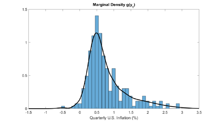
Figure 1: Estimated Marginal Distribution of U.S. Quarterly Inflation. The histogram is of observations of quarterly U.S. inflation between 1954:Q1 and 2020:Q2 computed as the quarterly differences of the logarithm of the GDP price deflator. The line is the adaptive KDE estimate of time-invariant marginal $G=F_{Y_{t}}$.

Copula parameter estimation

The parameters of this time series copula model are estimated using their Bayesian posterior with the prior $\pi_{\theta}(\text{\boldmath$\theta$})\propto\frac{1}{\sigma^{2}_{\mu}\sigma^{2}_{\zeta}}\mathds{1}(\text{\boldmath$\theta$}\in R_{\theta})$, where $R_{\theta}$ is the region of parameter values that correspond to the constraints outlined above. Algorithm 2 can be used to estimate the copula parameters, where at Step 1 the state vector $x$ is partitioned into $\bm{\mu}=(\mu_{1},\ldots,\mu_{T})^{\top}$ and $\bm{\zeta}=(\zeta_{1},\ldots,\zeta_{T})^{\top}$, and generated using the two separate steps:

• Step 1a. Generate from $f(\bm{\mu}|\bm{\theta},\bm{\zeta},\bm{y})\propto\prod_{t=1}^{T}\phi_{1}\left(z_{t};\mu_{t},\exp(\zeta_{t})\right)f(\bm{\mu}|\bm{\theta})$

• Step 1b. Generate from $f(\bm{\zeta}|\bm{\theta},\bm{\mu},\bm{y})\propto\prod_{t=1}^{T}\phi_{1}\left(z_{t};\mu_{t},\exp(\zeta_{t})\right)f(\bm{\zeta}|\bm{\theta})$

The posterior of $\bm{\mu}$ in Step 1a can be recognized as normal with zero mean and a band one precision matrix, so that generation is both straightforward and fast. There are a number of efficient methods to generate $\bm{\zeta}$ in Step 1b in the literature, and the fast “precision sampler” for the latent states outlined in Chan and Jeliazkov (2009) is used here. In Step 2 of the sampler, a normal approximation is used as a proposal density for the Metropolis-Hastings step, which has high acceptance rates in practice.

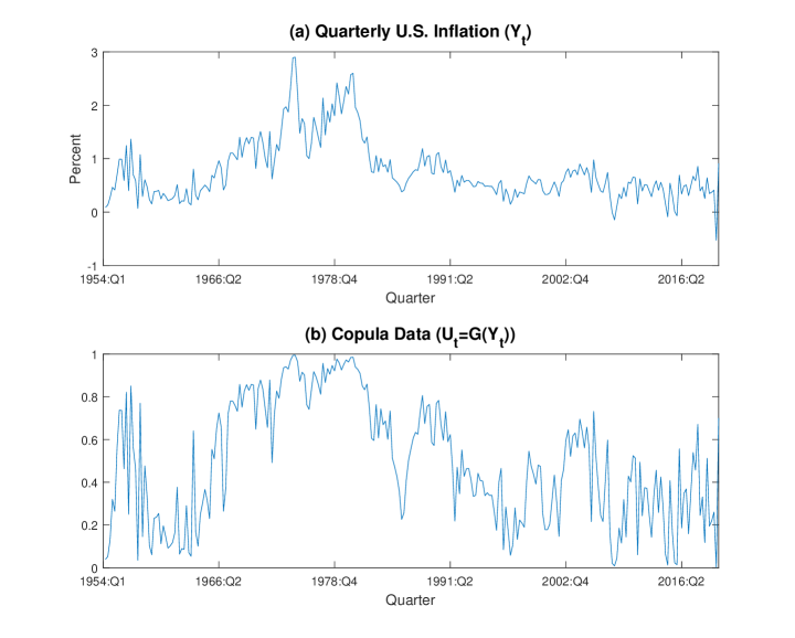
Figure 2: U.S. Inflation and Copula Data. Panel (a) plots the $T=266$ observations of U.S. quarterly inflation. Panel (b) plots the corresponding copula data $u_{t}=G(y_{t})$. The impact of the COVID-19 pandemic is seen in the last two observations.

Empirical results

The adaptive kernel density estimator (AKDE) of Shimazaki and Shinomoto (2010) is used to estimate a time-invariant marginal distribution $G$ of $Y_{t}$, and is presented in Figure 1. The estimated density is smooth, positively skewed, and heavy-tailed; it accounts for both high (e.g. $2.9\%$ in 1974:Q3) and low (e.g. $-0.529\%$ in 2020:Q1) values. Figure 2 plots the time series, plus the copula data $u_{t}=G(y_{t})$ for $t=1,\ldots,T$.

To summarize the posterior estimate of the implicit copula, Figure 3 plots the posterior means and 90% posterior intervals for $\mu$ and $\exp(\text{\boldmath$\zeta$}/2)$, which are the mean and standard deviation of the auxiliary vector $\bm{Z}$. While these are not the mean and standard deviation of $\bm{Y}$, they do account for movements in the moments of this variable, and the impact of the Covid-19 pandemic on 2020 can be seen as a sharp jump in $\exp(\zeta_{t}/2)$ in panel (a), while the inflationary period of the 1970’s can be see in high values of $\mu_{t}$ in panel (b).

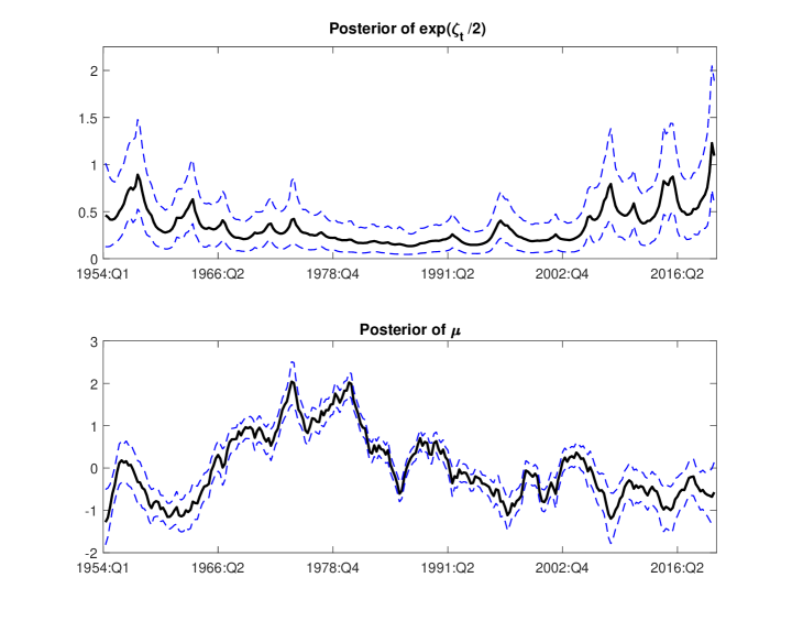
Figure 3: Bayesian posterior estimates of the latent states. Panel (a) plots $\exp(\text{\boldmath$\zeta$}/2)$ and panel (b) $\mu$. The posterior mean is the solid line, and the dashed lines are the 5% and 95% posterior quantiles.

There is high serial dependence in both state variables. One way to show how this affects the time series copula is to consider the bivariate margin $c_{t-1:t}(u_{t-1},u_{t}|\text{\boldmath$\theta$})$ of the copula density, which is time invariant. It is given by $c_{1:2}(u_{1},u_{2}|\text{\boldmath$\theta$})=f_{Z_{1:2}}(z_{1},z_{2}|\text{\boldmath$\theta$})/f_{Z_{1}}(z_{1}|\text{\boldmath$\theta$})f_{Z_{1}}(z_{2}|\text{\boldmath$\theta$})$, where the numerator is computed by numerical integration. Figure 4 plots this density at the posterior mean of the copula parameters $\theta$, and two interesting features can be seen. First, “spikes” at the corners (i.e. near (0,0), (0,1), (1,0) and (1,1)) are indicative of strong dependence in the volatility of the series; see Loaiza-Maya et al. (2018) and Bladt and McNeil (2021) for a discussion of such a pattern in a time series copula. Second, the positive “ridge” running from (0,0) to (1,1) is indicative of positive dependence in the level of the series. Both these features are well-known aspects of inflation time series, and the implicit copula captures them both while also allowing for the asymmetric marginal distribution in Figure 1. The time series copula model therefore allows for more realistic modeling of tail risk than the standard UCSV model, and improves density forecast accuracy, including in the tails.

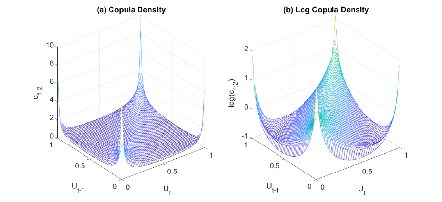
Figure 4: Panel (a) bivariate marginal copula density $c_{t-1:t}(u_{t-1},u_{t})$ evaluated at the posterior mean of $\theta$ (the values of which are $\hat{\rho}_{\zeta}=0.896$, $\hat{\sigma}_{\zeta}^{2}=0.407$, $\hat{\rho}_{\mu}=0.960$ and $\hat{\sigma}_{\mu}^{2}=0.059$). Panel (b) presents the same density on the logarithmic scale. The spikes in the four corners are indicative of serial dependence in the variance of the series. The ridge from (0,0) to (1,1) is indicative of serial dependence in the level of the series.

5 Implicit copulas for multivariate time series

Copulas have been used extensively to capture cross-sectional dependence in a multivariate stochastic process $\{\bm{Y}_{t}\}$, where $\bm{Y}_{t}=(Y_{1,t},\ldots,Y_{d,t})^{\top}$; see Patton (2006), Rodriguez (2007), Hafner and Manner (2012) and Creal and Tsay (2015) for just some examples. These models typically capture serial dependence through existing marginal time series models; for example, heteroscedastic models are normally used for financial returns. An alternative is to use a single high-dimensional—but parsimonious—copula to capture both serial and cross-sectional dependence jointly. An advantage of this approach is that the marginal distribution of each variable can be modeled directly, including as non-parametric. It is this type of time series copula that is the focus of this section.

5.1 Multivariate time series copula models

5.1.1 Copula model

If the random vector $\bm{Y}=(\bm{Y}_{1}^{\top},\ldots,\bm{Y}_{T}^{\top})^{\top}$, then $F_{Y}$ is given by (1) with $m=Td$ and the order of the elements of $\bm{Y}$ determines the interpretation of $C$. If all variables are continuous, $f_{Y}$ is given by (2), so that

$$f_{Y}(\text{\boldmath$y$})=c(\bm{u})\prod_{j=1}^{d}\prod_{t=1}^{T}f_{Y_{j,t}}(y_{j,t})\,,$$ (19)

where $\text{\boldmath$y$}=(\text{\boldmath$y$}_{1}^{\top},\ldots,\text{\boldmath$y$}_{T}^{\top})^{\top}$, $\text{\boldmath$y$}_{t}=(y_{1,t},\ldots,y_{d,t})^{\top}$, $\text{\boldmath$u$}=(\text{\boldmath$u$}_{1}^{\top},\ldots,\text{\boldmath$u$}_{T}^{\top})^{\top}$ and $\text{\boldmath$u$}_{t}=(u_{1,t},\ldots,u_{d,t})^{\top}$. For discrete-valued variables the mass function is given by (3), and an extended likelihood for $(\bm{Y},\bm{U})$ is given by (4); see Loaiza-Maya and Smith (2019). Marginal models for each of the $d$ series are required, and one option is to assume they are time-invariant with distribution functions $G_{1},\ldots,G_{d}$, which can be estimated separately.

5.1.2 Copula choice

Selecting an appropriate $Td$-dimensional copula with density $c$ at (19) is difficult because it needs to capture three forms of dependence: (i) cross-sectional contemporaneous, (ii) within-series serial, and (iii) cross-series serial. One solution is to use a vine copula; for example see Brechmann and Czado (2015) for the two-dimensional case, Smith (2015) and Loaiza-Maya et al. (2018) for D-vine copulas, Beare and Seo (2015) for an M-vine and Zhao et al. (2020) for an alternative vine-based copula; see also Rémillard et al. (2012); Nagler et al. (2020). However, implicit copulas constructed from existing multivariate time series models offer a tractable alternative to vines, particularly for series where $T$ and/or $d$ are large.

5.2 Gaussian vector autoregression copula

The most popular implicit copula for multivariate time series is that of a Gaussian vector autoregression (VAR) for $\{\bm{Z}_{t}\}$. This is an extension of the autoregression copula in Section 4.2.4. Consider the following VAR with lag $p$,

$$\bm{Z}_{t}=\sum_{j=1}^{p}B_{j}\bm{Z}_{t-j}+\text{\boldmath$e$}_{t}\,,\mbox{ where }\text{\boldmath$e$}_{t}\sim N(\bm{0},\Sigma)\,.$$ (20)

The mean is set to zero because it is unidentified in the copula, and the variances are fixed so that $\mbox{Var}(Z_{j,t})=1$. Then $\bm{Z}=(\bm{Z}_{1}^{\top},\ldots,\bm{Z}_{T}^{\top})^{\top}\sim N_{Td}(\bm{0},\Omega)$, where $\Omega$ is the block Toeplitz correlation matrix of this process. This is a matrix of $(T\times T)$ blocks, with the $(s,t)$th block being given by $\Omega_{h}\equiv\mbox{Corr}(\bm{Z}_{t+h},\bm{Z}_{t})$ for $h=|t-s|$ and $t\geq s$; for example, see Lütkepohl (2005, p.30). Because the Gaussian copula is closed under marginalization, the $d$-dimensional marginal distribution in $\bm{Y}_{t}$ also has a Gaussian copula function $C_{\mbox{\tiny Ga}}(\text{\boldmath$u$}_{t};\Omega_{0})$. For example, for continuous data $f_{Y_{t}}(\text{\boldmath$y$}_{t})=c_{\mbox{\tiny Ga}}(\text{\boldmath$u$}_{t};\Omega_{0})\prod_{j=1}^{d}f_{Y_{j,t}}(y_{j,t})$.

For continuous time series, a straightforward approach to estimate the model is to first estimate appropriate marginal distributions $F_{Y_{j,t}}$; for example, by assuming time-invariance in the marginals and applying a kernel density estimator to each of the $d$ series. Second, compute the auxiliary data $z_{j,t}=\Phi^{-1}(F_{Y_{j,t}}(y_{j,t}))$ for $i=1,\ldots,d$ and $t=1,\ldots,T$. Third, apply standard likelihood-based methods for Gaussian VARs directly to this auxiliary data to estimate the unknown parameters $B_{1},\ldots,B_{p},\Sigma$. From these $\Omega$ can be computed, although this can be impractical to evaluate when $m=Td$ is large and there is often no need to do so.

The conditional density for $\bm{Y}_{t+1}|\bm{Y}_{1:t}$ can be derived in a similar manner as for the univariate autoregression copula model. This is given by

$$f_{Y_{t+1|1:t}}(\text{\boldmath$y$}_{t+1}|\text{\boldmath$y$}_{1},\ldots,\text{\boldmath$y$}_{t}) = f_{Z_{t+1|1:t}}(\text{\boldmath$z$}_{t+1}|\text{\boldmath$z$}_{1},\ldots,\text{\boldmath$z$}_{t})\frac{f_{Y_{t+1}}(\text{\boldmath$y$}_{t+1})}{f_{Z_{t+1}}(\text{\boldmath$z$}_{t+1})}$$

$$= \phi_{d}\left(\text{\boldmath$z$}_{t+1};\sum_{j=1}^{p}B_{j}\bm{Z}_{t-j},\Sigma\right)\frac{c_{\mbox{\tiny Ga}}(\bm{u}_{t+1};\Omega_{0})\prod_{j=1}^{d}g_{j}(y_{j,t+1})}{\phi_{d}(\text{\boldmath$z$}_{t+1};\bm{0},\Omega_{0})}$$

where time-invariant marginal densities $g_{1},\ldots,g_{d}$ are assumed. Drawing from this conditional distribution is straightforward by first simulating $\bm{Z}_{t+1}$ directly from (20), and then transforming to a draw $\bm{Y}_{t+1}=(G_{1}^{-1}(\Phi(Z_{1,t+1})),\ldots,G_{d}^{-1}(\Phi(Z_{d,t+1})))^{\top}$, which can be used to compute the predictive distribution.

5.2.1 Further reading

Biller and Nelson (2003) were the first to construct the Gaussian VAR copula via transformation, but did not recognize it as a Gaussian copula and called it a “Vector-Autoregressive-To-Anything” distribution. Smith (2015) and Smith and Vahey (2016) also consider this Gaussian copula model, its D-vine representation and apply it to multivariate macroeconomic and financial forecasting. Similar to the univariate case, the Gaussian VAR copula model can capture a degree of heteroscedasticity in the time series given a suitable choice of marginal distributions $G_{1},\ldots,G_{d}$ for the $d$ time series; see Smith and Vahey (2016) for a demonstration. There is also a growing interest in multivariate times series copulas in machine learning. For example, Salinas et al. (2019) construct a Gaussian copula from low rank factor decomposition where the small number of factors follow a Gaussian process with recurrent neural network (RNN) dynamics. Klein et al. (2020) propose constructing a Gaussian copula process that is constructed as the implicit copula of an RNN with Gaussian errors.

Existing econometric applications of multivariate time series often have parameters that vary over time (widely called a “dynamic” model) along with substantial regularization; see Bitto and Frühwirth-Schnatter (2019), Huber et al. (2020) and references therein. These features can also be employed for the parameters of implicit copulas. For example, Smith and Vahey (2016) use Bayesian selection on the D-vine representation of the Gaussian VAR copula for regularization, Creal and Tsay (2015), Oh and Patton (2017) and Opschoor et al. (2020) allow the parameters of elliptical copulas to vary over time, and Oh and Patton (2020) consider a dynamic skew $t$ copula. In another approach Loaiza-Maya et al. (2018) extend the UCSV model in Section 4.3.3 to the multivariate case and show how to construct its implicit copula. In all these studies, the copula models are more accurate than non-copula benchmarks, and the implicit copulas used are scalable to high dimensions.

6 Regression copula processes

Copula models with regression margins have been used widely; for examples, see Pitt et al. (2006), Song et al. (2009), Masarotto et al. (2012) and Klein and Kneib (2016). However, another usage of a copula with regression data is to capture the dependence between multiple observations on a single dependent variable $Y$, conditional on the covariate values. This defines a copula process (Wilson and Ghahramani, 2010) on the covariate space, which Smith and Klein (2021) call a “regression copula”. When combined with a flexible marginal distribution for $Y$, it specifies a new distributional regression model. This is where the covariates affect the entire distribution of $Y$. Klein and Smith (2019) and Smith and Klein (2021) consider a regression copula that is the implicit copula of the joint distribution of observations in an auxiliary regression model. They are inherently high dimensional, yet can be estimated in reasonable time using Bayesian methods. The idea is outlined in this section for continuous $Y$, and greater detail can be found in these papers.

6.1 The basic idea of a regression copula

6.1.1 The copula process model

Consider $N>1$ realizations $\bm{Y}_{1:N}=(Y_{1},\ldots,Y_{N})^{\top}$ of a dependent variable with corresponding values $\text{\boldmath$x$}_{1:N}=\{\text{\boldmath$x$}_{1},\ldots,\text{\boldmath$x$}_{N}\}$ for $p$ covariates, with $\text{\boldmath$x$}_{i}=(x_{i,1},\ldots,x_{i,p})^{\top}$. Then application of Sklar’s theorem to the distribution of $\bm{Y}_{1:N}|\text{\boldmath$x$}_{1:N}$ gives

$$F_{Y_{1:N}}(\text{\boldmath$y$}_{1:N}|\text{\boldmath$x$}_{1:N})=C^{\dagger}_{1:N}\left(F_{Y_{1}}(y_{1}|\text{\boldmath$x$}_{1}),\ldots,F_{Y_{N}}(y_{N}|\text{\boldmath$x$}_{N})\,;\,\text{\boldmath$x$}_{1:N}\right)\,.$$

The $N$-dimensional copula function $C^{\dagger}_{1:N}(\cdot\,;\,\text{\boldmath$x$}_{1:N})$ is a copula process on the covariate space, and $F_{Y_{i}}(y_{i}|\text{\boldmath$x$}_{i})$ is the distribution function of $Y_{i}|\text{\boldmath$x$}_{i}$. Both are typically unknown, and in a copula model these are selected to define the distribution. One tractable but effective simplification is to allow the covariates to only affect the dependent variable through the copula function, so that $Y_{i}$ is marginally independent of $\text{\boldmath$x$}_{i}$. In this case,

$$F_{Y_{1:N}}(\text{\boldmath$y$}_{1:N}|\text{\boldmath$x$}_{1:N})=C_{1:N}\left(F_{Y_{1}}(y_{1}),\ldots,F_{Y_{N}}(y_{N})\,;\,\text{\boldmath$x$}_{1:N},\text{\boldmath$\theta$}\right)\,,$$ (21)

with $\theta$ unknown copula parameters that are unaffected by the dimension $N$ and require estimation. Here, the joint distribution of $\bm{Y}_{1:N}$ is dependent on $\text{\boldmath$x$}_{1:N}$ via the copula, so that the conditional distribution $Y_{N}|(\bm{Y}_{1:N-1}=\text{\boldmath$y$}_{1:N-1}),\text{\boldmath$x$}_{1:N}$ is also. The latter is employed as the predictive distribution of the regression model, as discussed further below.

When the dependent variable is continuous, the joint density is

$$f_{Y_{1:N}}(\text{\boldmath$y$}_{1:N}|\text{\boldmath$x$}_{1:N})=c_{1:N}(u_{1},\ldots,u_{N}\,;\,\text{\boldmath$x$}_{1:N},\text{\boldmath$\theta$})\prod_{i=1}^{N}f_{Y_{i}}(y_{i})\,,$$ (22)

with $u_{i}=F_{Y_{i}}(y_{i})$. An advantage (that is also in common with the time series copula models discussed in Section 4) is that if $F_{Y_{i}}(y_{i})\equiv G(y_{i})$ is assumed to be invariant with respect to the index $i$, then $G$ can be estimated using non-parametric or other flexible estimators. The remaining component of the copula model at (21) is the choice of copula process, which is aptly called a regression copula because it is a function of $\text{\boldmath$x$}_{1:N}$.

6.1.2 Distributional regression

To see how (22) defines a distributional regression model, consider the predictive density for a continuous-valued dependent variable. For a sample of size $n$ with covariate values $\text{\boldmath$x$}_{1:n}$ and dependent variable values $\bm{Y}_{1:n}=\text{\boldmath$y$}_{1:n}$ arising from (22), the predictive distribution of the subsequent value $Y_{n+1}$ with observed covariates $\text{\boldmath$x$}_{n+1}$ is defined to be that of $Y_{n+1}|\text{\boldmath$x$}_{1:n+1},\text{\boldmath$y$}_{1:n}$, which has density

$$f_{\mbox{\tiny pred}}(y_{n+1}|\text{\boldmath$x$}_{n+1},\text{\boldmath$\theta$}) \equiv f(y_{n+1}|\text{\boldmath$x$}_{1:n+1},\text{\boldmath$y$}_{1:n},\text{\boldmath$\theta$})=\frac{f(\text{\boldmath$y$}_{1:n+1}|\text{\boldmath$x$}_{1:n+1},\text{\boldmath$\theta$})}{f(\text{\boldmath$y$}_{1:n}|\text{\boldmath$x$}_{1:n},\text{\boldmath$\theta$})}$$ (23)

$$= \frac{c_{1:n+1}(u_{1},\ldots,u_{n+1};\text{\boldmath$x$}_{1:n+1},\text{\boldmath$\theta$})}{c_{1:n}(u_{1},\ldots,u_{n};\text{\boldmath$x$}_{1:n},\text{\boldmath$\theta$})}f_{Y_{n+1}}(y_{n+1})$$

$$= f(u_{n+1}|\text{\boldmath$u$}_{1:n},\text{\boldmath$x$}_{1:n+1},\text{\boldmath$\theta$})f_{Y_{n+1}}(y_{n+1})\,.$$

Thus, the predictive density is a function of the covariate vector $\text{\boldmath$x$}_{n+1}$, as well as those of the sample $\text{\boldmath$x$}_{1:n}$. Moreover, the entire distribution (not just the first or other moments of $Y_{n+1}$) is a function of $\text{\boldmath$x$}_{n+1}$ as illustrated empirically in Section 6.3.4.

6.2 Implicit regression copula process

One regression copula process $C_{1:N}$ that can be used at (21) is an implicit copula derived from an existing regression model, as now discussed.

6.2.1 The copula

Implicit regression copulas are constructed as in Section 2, but when also conditioning on the covariate values; i.e. from an “auxiliary regression” model. Consider a regression model for the auxiliary vector $\bm{Z}_{1:N}=(Z_{1},\ldots,Z_{N})^{\top}$ with covariate values $\text{\boldmath$x$}_{1:N}$ and parameter vector $\theta$. Denote the joint distribution function of $\bm{Z}_{1:N}|\text{\boldmath$x$}_{1:N},\text{\boldmath$\theta$}$ as $F_{Z_{1:N}}(\cdot|\text{\boldmath$x$}_{1:N},\text{\boldmath$\theta$})$, with $i$th marginal $F_{Z_{i}}(\cdot|\text{\boldmath$x$}_{i},\text{\boldmath$\theta$})$. Then, extending the definition in Table 1, the following transformations define a regression copula model

$$U_{i}=F_{Z_{i}}(Z_{i}|\text{\boldmath$x$}_{i},\text{\boldmath$\theta$})\,,\mbox{ and }Y_{i}=F_{Y_{i}}^{-1}(U_{i})\,.$$

If $\text{\boldmath$z$}_{1:N}=(z_{1},\ldots,z_{N})^{\top}$, $z_{i}=F_{Z_{i}}^{-1}(u_{i}|\text{\boldmath$x$}_{i},\text{\boldmath$\theta$})$ and $m=N$, then the implicit copula function at (5) and density at (6) for this model are given by

$$C_{Z_{1:N}}(\text{\boldmath$u$}_{1:N};\text{\boldmath$x$}_{1:N},\text{\boldmath$\theta$}) \equiv F_{Z_{1:N}}\left(F_{Z_{1}}^{-1}(u_{1}|\text{\boldmath$x$}_{1},\text{\boldmath$\theta$}),\ldots,F_{Z_{N}}^{-1}(u_{N}|\text{\boldmath$x$}_{N},\text{\boldmath$\theta$})|\text{\boldmath$x$}_{1:N},\text{\boldmath$\theta$}\right)\,,$$ (24)

$$c_{Z_{1:N}}(\text{\boldmath$u$}_{1:N};\text{\boldmath$x$}_{1:N},\text{\boldmath$\theta$}) \equiv \frac{f_{Z_{1:N}}(\text{\boldmath$z$}_{1:N}|\text{\boldmath$x$}_{1:N},\text{\boldmath$\theta$})}{\prod_{i=1}^{N}f_{Z_{i}}(z_{i}|\text{\boldmath$x$}_{i},\text{\boldmath$\theta$})}\,.$$ (25)

In (25) $f_{Z_{i}}(z_{i}|\text{\boldmath$x$}_{i},\text{\boldmath$\theta$})$ is the density function of the auxiliary variable $Z_{i}$, conditional on the covariates $\text{\boldmath$x$}_{i}$. These expressions for $C_{Z_{1:N}}$ and $c_{Z_{1:N}}$ can then be used in (21) and (22) to specify a distributional regression.

If in the auxiliary regression $f_{Z_{1:N}}(\text{\boldmath$z$}_{1:N}|\text{\boldmath$x$}_{1:N},\text{\boldmath$\theta$})=\prod_{i=1}^{N}f_{Z_{i}}(z_{i}|\text{\boldmath$x$}_{i},\text{\boldmath$\theta$})$, then from (25) the implicit copula is the trivial independence copula. Thus, only distributions where $\bm{Z}_{1:N}$ are dependent are useful for constructing an implicit regression copula, as in Section 6.3 below.

6.2.2 Predictive density

Employing the copula density at (25) for that in the predictive density at (23), gives the following:

$$f_{\mbox{\tiny pred}}(y_{n+1}|\text{\boldmath$x$}_{n+1},\text{\boldmath$\theta$}) = \frac{f_{Z_{1:n+1}}(\text{\boldmath$z$}_{1:n+1}|\text{\boldmath$x$}_{1:n+1},\text{\boldmath$\theta$})}{f_{Z_{1:n}}(\text{\boldmath$z$}_{1:n}|\text{\boldmath$x$}_{1:n},\text{\boldmath$\theta$})f_{Z_{n+1}}(z_{n+1}|\text{\boldmath$x$}_{n+1},\text{\boldmath$\theta$})}f_{Y_{n+1}}(y_{n+1})$$ (26)

$$= f_{Z_{n+1|1:n}}(z_{n+1}|\text{\boldmath$z$}_{1:n},\text{\boldmath$x$}_{1:n+1},\text{\boldmath$\theta$})\frac{f_{Y_{n+1}}(y_{n+1})}{f_{Z_{n+1}}(z_{n+1}|\text{\boldmath$x$}_{n+1},\text{\boldmath$\theta$})}\,.$$

To evaluate (26) in practice, a point estimate of $\theta$ can be used. In a Bayesian analysis another option exists, where $\theta$ is integrated out with respect to its posterior density $f(\text{\boldmath$\theta$}|\text{\boldmath$y$})$ to obtain

$$f_{\mbox{\tiny pred}}^{\mbox{\tiny Bayes}}(y_{n+1}|\text{\boldmath$x$}_{n+1})=\int f_{\mbox{\tiny pred}}(y_{n+1}|\text{\boldmath$x$}_{n+1},\text{\boldmath$\theta$})f(\text{\boldmath$\theta$}|\text{\boldmath$y$})\mbox{d}\text{\boldmath$\theta$}\,.$$

This is called the “posterior predictive density”, and evaluation of the integral is usually undertaken using draws obtained from an MCMC sampling scheme.

6.3 Linear regression copula

In principle, implicit copula processes outlined above can be constructed from a wide range of different regression models. Klein and Smith (2019) suggest doing so for a Gaussian linear regression, as now outlined.

6.3.1 The copula

For a dependent variable $\widetilde{Z}_{i}$, consider the linear regression

$$\widetilde{Z}_{i}=\text{\boldmath$x$}_{i}^{\top}\text{\boldmath$\beta$}+\sigma e_{i}\,,$$

with $e_{i}$ distributed independently $N(0,1)$. Conditional on both $\text{\boldmath$x$}_{i}$ and the parameters $\text{\boldmath$\beta$},\sigma^{2}$, the elements of $\widetilde{\bm{Z}}_{1:N}=(\widetilde{Z}_{1},\ldots,\widetilde{Z}_{N})^{\top}$ are distributed independently, so that their joint distribution cannot be used directly to specify a useful regression copula with density at (25). However, a Bayesian framework can be employed where $\beta$ is treated as random and marginalized out of the distribution for $\widetilde{\bm{Z}}_{1:N}$, the elements of which are then dependent. From this distribution a useful implicit regression copula can be formed as below.

If $B=[\text{\boldmath$x$}_{1}|\text{\boldmath$x$}_{2}|\cdots|\text{\boldmath$x$}_{N}]^{\top}$ is the $(N\times p)$ regression design matrix, then the regression can be written as the linear model

$$\widetilde{\bm{Z}}_{1:N}|\text{\boldmath$x$}_{1:N},\text{\boldmath$\beta$},\sigma^{2}\sim N(B\text{\boldmath$\beta$},\sigma^{2}I).$$ (27)

The conjugate proper prior

$$\text{\boldmath$\beta$}|\sigma^{2}\sim N(\bm{0},\sigma^{2}P(\text{\boldmath$\theta$})^{-1})\,,$$ (28)

is used, where the precision matrix $P(\text{\boldmath$\theta$})$ is of full rank $p$ and a function of $\theta$. It is necessary to assume a proper prior for $\beta$, because it ensures that the distribution with $\beta$ integrated out is also proper. Doing so (by recognizing a normal in $\beta$) gives

$$\widetilde{\bm{Z}}_{1:N}|\text{\boldmath$x$}_{1:N},\text{\boldmath$\theta$},\sigma^{2}\sim N\left(\bm{0},\sigma^{2}(I-B\Sigma B^{\top})^{-1}\right)\,,$$ (29)

with $\Sigma=(B^{\top}B+P(\text{\boldmath$\theta$}))^{-1}$. Application of the Woodbury formula further simplifies the variance matrix at (29) as

$$\sigma^{2}(I-B\Sigma B^{\top})^{-1}=\sigma^{2}\left(I+BP(\text{\boldmath$\theta$})^{-1}B^{\top}\right)\,.$$

The variance of an individual observation $i$ is the $i$th leading diagonal element of this matrix, so that $\mbox{Var}(\widetilde{Z}_{i}|\text{\boldmath$x$}_{i},\text{\boldmath$\theta$},\sigma^{2})=\sigma^{2}(1+\text{\boldmath$x$}_{i}^{\top}P(\text{\boldmath$\theta$})^{-1}\text{\boldmath$x$}_{i})$.

The copula of any normal distribution is the Gaussian copula discussed in Section 3.1. The parameter matrix $R$ is the correlation matrix of (29), and it is obtained by standardizing $\widetilde{Z}_{i}$ to have unit variance as follows. Let $s_{i}=(1+\text{\boldmath$x$}_{i}^{\top}P(\text{\boldmath$\theta$})^{-1}\text{\boldmath$x$}_{i})^{-1/2}$, then define the auxiliary variable of the implicit copula as $Z_{i}=\frac{s_{i}}{\sigma}\widetilde{Z}_{i}$. Thus, if the diagonal matrix $S(\text{\boldmath$x$}_{1:N},\text{\boldmath$\theta$})=\mbox{diag}(s_{1},\ldots,s_{N})$, then from (29) the conditional distribution of $\bm{Z}_{1:N}=(Z_{1},\ldots,Z_{N})^{\top}$ is $\bm{Z}_{1:N}|\text{\boldmath$x$}_{1:N},\text{\boldmath$\theta$},\sigma^{2}\sim N\left(\bm{0},R\right)$ with correlation matrix

$$R(\text{\boldmath$x$}_{1:N},\text{\boldmath$\theta$})=S(\text{\boldmath$x$}_{1:N},\text{\boldmath$\theta$})\left(I+BP(\text{\boldmath$\theta$})^{-1}B^{\top}\right)S(\text{\boldmath$x$}_{1:N},\text{\boldmath$\theta$})\,,$$ (30)

and has copula function $C_{\mbox{\tiny Ga}}(\text{\boldmath$u$};R)$. This is a copula process on the covariate space because $R$ is a function of the covariate vector $\text{\boldmath$x$}_{1:N}$ (the notation $R$ and $R(\text{\boldmath$x$}_{1:N},\text{\boldmath$\theta$})$ is used interchangeably here.) The parameter $\sigma^{2}$ does not feature in $R$ and is unidentified in the copula, so that $\sigma^{2}=1$ can be assumed throughout.

Example: horseshoe regularization

Different implicit copulas can be constructed by using different conditionally Gaussian priors for $\beta$ at (28). Klein and Smith (2019) explore three different choices, including the horseshoe prior of Carvalho and Polson (2010) which is outlined here. This prior provides regularization of $\beta$ in the auxiliary regression. The prior is given by

$$\text{\boldmath$\beta$}|\text{\boldmath$\lambda$},\tau \sim N\left(\bm{0},\mbox{diag}(\text{\boldmath$\lambda$})^{2}\right)\,,\;\text{\boldmath$\lambda$}=(\lambda_{1},\ldots,\lambda_{p})^{\top}\,,$$

$$\lambda_{j}|\tau \sim \mbox{Half-Cauchy}(0,\tau)\,,\mbox{ and }\tau\sim\mbox{Half-Cauchy}(0,1)\,,$$

see Polson and Scott (2012). The hyper-parameters of this prior are the parameters of the implicit copula $\text{\boldmath$\theta$}=(\text{\boldmath$\lambda$}^{\top},\tau)^{\top}$, while the precision matrix $P(\text{\boldmath$\theta$})=\mbox{diag}(\text{\boldmath$\lambda$})^{-2}$ is diagonal.

6.3.2 Estimation

For a sample of $n$ observations, from (22) and (25), the likelihood is

$$f_{Y_{1:n}}(\text{\boldmath$y$}_{1:n}|\text{\boldmath$x$}_{1:n},\text{\boldmath$\theta$})=f_{Z_{1:n}}(\text{\boldmath$z$}_{1:n}|\text{\boldmath$x$}_{1:n},\text{\boldmath$\theta$})\prod_{i=1}^{n}\frac{f_{Y_{i}}(y_{i})}{f_{Z_{i}}(z_{i}|\text{\boldmath$x$}_{i},\text{\boldmath$\theta$})}=\phi_{n}\left(\text{\boldmath$z$}_{1:n};\bm{0},R(\text{\boldmath$x$}_{1:n},\text{\boldmath$\theta$})\right)\prod_{i=1}^{n}\frac{g(y_{i})}{\phi(z_{i})}\,,$$

for an invariant marginal distribution with density $f_{Y_{i}}=g$. However, even though the likelihood is available in closed form, for large $n$ evaluating and inverting the $(n\times n)$ matrix $R(\text{\boldmath$x$}_{1:n},\text{\boldmath$\theta$})$ to compute the likelihood is computationally demanding.

Instead, it is more efficient to use the likelihood also conditional on $\beta$, and integrate out $\beta$ using an MCMC scheme. (It is stressed here that doing so does not change the implicit copula specification.) First, note that from (27) when also conditioning on $\beta$ the vector $\bm{Z}_{1:n}=S\widetilde{\bm{Z}}_{1:n}\sim N(SB\text{\boldmath$\beta$},S^{2})$ (with $\sigma^{2}=1$ and $S=S(\text{\boldmath$x$}_{1:n},\text{\boldmath$\theta$})$). Also, the Jacobian of the transformation from $\bm{Z}_{1:n}$ to $\bm{Y}_{1:n}$ is $J_{Z_{1:n}\rightarrow Y_{1:n}}=\prod_{i=1}^{n}g(y_{i})/\phi(z_{i})$. Then, by a change of variables, the likelihood also conditional on $\beta$ is

$$f(\text{\boldmath$y$}_{1:n}|\text{\boldmath$x$}_{1:n},\text{\boldmath$\beta$},\text{\boldmath$\theta$})=f(\text{\boldmath$z$}_{1:n}|\text{\boldmath$x$}_{1:n},\text{\boldmath$\beta$},\text{\boldmath$\theta$})J_{Z_{1:n}\rightarrow Y_{1:n}}=\phi_{n}(\text{\boldmath$z$}_{1:n};SB\text{\boldmath$\beta$},S^{2})\prod_{i=1}^{n}\frac{g(y_{i})}{\phi(z_{i})}\,,$$ (31)

which can be evaluated in $O(n)$ operations because $S$ is a diagonal matrix. A Bayesian approach that employs this conditional likelihood, evaluates the augmented posterior $f(\text{\boldmath$\beta$},\text{\boldmath$\theta$}|\text{\boldmath$y$}_{1:n})$ using the sampler at 3. Implementation details for this sampler are given in Klein and Smith (2019).

Algorithm 3 (MCMC sampler for regression copula)

• Generate from $\text{\boldmath$\beta$}|\text{\boldmath$x$}_{1:n},\text{\boldmath$\theta$},\text{\boldmath$y$}_{1:n}$ (which is a Gaussian distribution)

• Generate from $\text{\boldmath$\theta$}|\text{\boldmath$x$}_{1:n},\text{\boldmath$\beta$},\text{\boldmath$y$}_{1:n}$

6.3.3 Prediction

One way to compute the predictive density that avoids computing $R(\text{\boldmath$x$}_{1:n},\text{\boldmath$\theta$})$ or its inverse (and is therefore faster than alternatives), is to also condition on $\beta$. By a change of variables from $Y_{n+1}$ to $Z_{n+1}$,

$$f(y_{n+1}|\text{\boldmath$x$}_{1:n+1},\text{\boldmath$\beta$},\text{\boldmath$\theta$})=f(z_{n+1}|\text{\boldmath$x$}_{1:n+1},\text{\boldmath$\beta$},\text{\boldmath$\theta$})\frac{f_{Y_{n+1}}(y_{n+1})}{\phi(z_{n+1})}$$ (32)

$$=\phi_{1}\left(z_{n+1};s_{n+1}\text{\boldmath$x$}_{n+1}^{\top}\text{\boldmath$\beta$},s_{n+1}^{2}\right)\frac{f_{Y_{n+1}}(y_{n+1})}{\phi\left(z_{n+1}\right)}\,,$$

where $s_{n+1}=(1+\text{\boldmath$x$}_{n+1}^{\top}P(\text{\boldmath$\theta$})^{-1}\text{\boldmath$x$}_{n+1})^{-1/2}$ and $z_{n+1}=\Phi^{-1}(F_{Y_{n+1}}(y_{n+1}))$.

The draws for $\text{\boldmath$\beta$},\text{\boldmath$\theta$}$ from Algorithm 3 can be used to either integrate out $\text{\boldmath$\beta$},\text{\boldmath$\theta$}$ with respect to the augmented posterior, or to compute plug-in point estimates for $\beta$ and also $s_{n+1}$. If $F_{Y_{n+1}}$ is fixed to its estimate, and $\{\text{\boldmath$\beta$}^{[1]},\text{\boldmath$\theta$}^{[1]},\ldots,\text{\boldmath$\beta$}^{[J]},\text{\boldmath$\theta$}^{[J]}\}$ are the Monte Carlo draws, then the two Bayesian posterior estimators for the predictive density are:

$$\hat{f}^{\mbox{\tiny Bayes}}_{\mbox{\tiny pred}}(y_{n+1}|\text{\boldmath$x$}_{n+1}) \equiv \frac{1}{J}\sum_{j=1}^{J}f(y_{n+1}|\text{\boldmath$x$}_{1:n+1},\text{\boldmath$\beta$}^{[j]},\text{\boldmath$\theta$}^{[j]})\,,$$

$$\hat{f}^{\mbox{\tiny Point}}_{\mbox{\tiny pred}}(y_{n+1}|\text{\boldmath$x$}_{n+1}) \equiv \phi_{1}\left(z_{n+1};\hat{s}_{n+1}\text{\boldmath$x$}_{n+1}^{\top}\hat{\text{\boldmath$\beta$}},\hat{s}_{n+1}^{2}\right)\frac{f_{Y_{n+1}}(y_{n+1})}{\phi\left(z_{n+1}\right)}\,,$$

with

$$\hat{\text{\boldmath$\beta$}}=\frac{1}{J}\sum_{j=1}^{J}\text{\boldmath$\beta$}^{[j]}\,,\mbox{ and }\hat{s}_{n+1}=\frac{1}{J}\sum_{j=1}^{J}\left(1+\text{\boldmath$x$}_{n+1}^{\top}P(\text{\boldmath$\theta$}^{[j]})^{-1}\text{\boldmath$x$}_{n+1}\right)^{-1/2}\,.$$

In their empirical work, Klein and Smith (2019) and Smith and Klein (2021) found that estimates from these two estimators were very similar.

6.3.4 Empirical application: a non-Gaussian asset pricing model

Linear regression is widely used to estimate financial asset pricing models, where the dependent variable is the (excess) return on a stock. Yet stock returns are distributed far from Gaussian, so that a Gaussian regression model is mis-specified. To illustrate the regression copula model it is used to model monthly excess returns on American Express Company (which has NYSE ticker symbol “AXP”) using data from 07/1972 to 10/2020. The marginal distribution is assumed invariant with respect to observation, so that $F_{Y_{i}}(y_{i})=G(y_{i})$. A three parameter asymmetric Laplace distribution is fit, which better accounts for the distribution of returns as highlighted by Chen et al. (2012) and Taylor (2019). Figure 5 plots the density of the fitted margin, which is both asymmetric and has very heavy tails.

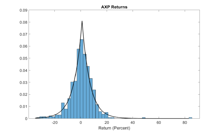
Figure 5: Histogram of $n=580$ AXP monthly excess returns between 07/1972 and 10/2020 in percent. The fitted asymmetric Laplace density used for the marginal density $f_{Y_{i}}(y_{i})=g(y_{i})$ is plotted as a black line.

The monthly values of the five factors suggested and described by Fama and French (2015) were used as covariates. These are market risk (MktRf), size (SMB), value (HML), profit (RMW) and investment (CMA) factors, with data obtained from Kenneth French’s website. The first three factors are widely employed, while the inclusion of the additional two factors RMW and CMA is more controversial. The linear regression copula constructed using the horseshoe prior for $\beta$ was estimated using Algorithm 3. Even though the implicit copula is of dimension $n=580$, employing the conditional likelihood at (31) means that estimation is tractable, with a computation time of only 32s to draw 10,000 iterates on a standard laptop.

Table 2: Posterior estimates of the regression copula model parameters for the American Express Company five factor asset pricing regression

Label	Covariate
	MktRf	SMB	HML	RMW	CMA
$\widehat{\text{\boldmath$\beta$}}$	0.1889	-0.0351	0.0441	-0.0020	-0.0303
95% Interval	(0.163,0.215)	(-0.067,-0.003)	(0.001,0.085)	(-0.031,0.024)	(-0.092,0.029)
$\widehat{\text{\boldmath$\lambda$}}$	0.0632	0.0316	0.0425	0.0203	0.1493
MH Acceptance Rate	85%	84%	84%	78%	85%

The first rows report the posterior mean of $\beta$ and the 95% posterior probability intervals for each covariate. The next rows report the posterior mean of $\lambda$, along with the Metropolis-Hasting (MH) acceptance rate for each element. In addition, the posterior mean of $\tau$ is 0.0715 with an MH acceptance rate of 92%.

Table 2 summarizes the posterior estimates of the coefficients $\beta$ and the regularization parameters $\lambda$. Of the five covariates, only the traditional three (MktRt, SMB and HML) were significant (“significant” here refers to the whether, or not, zero falls into the 95% posterior intervals for each coefficient $\beta_{i}$.) Thus, evidence for the inclusion of the two new factors RMW and CMA is weak. Also reported are the Metropolis-Hastings acceptance rates for the parameters. These are all high, suggesting Step 2 in Algorithm 3 is effective.

To illustrate the effect of the three significant covariates on the distribution of excess AXP returns, Figure 6 plots the predictive density (estimated using $\hat{f}^{\mbox{\tiny Bayes}}_{\mbox{\tiny pred}}$) for different values of each covariate, setting the other four covariates equal to their median values. For example, in panel (a) which focuses on variation in MktRf (the excess market return), the distribution is very different in location, spread, and shape for a typical month (MktRf=0.98) in comparison to a poor month ($\mbox{MktRf}=-9.35$) or a strong month ($\mbox{MktRf}=8.42$). This highlights that the regression copula process combined with $G$ defines a distributional regression model, where each covariate affects the entire distribution of $Y$.

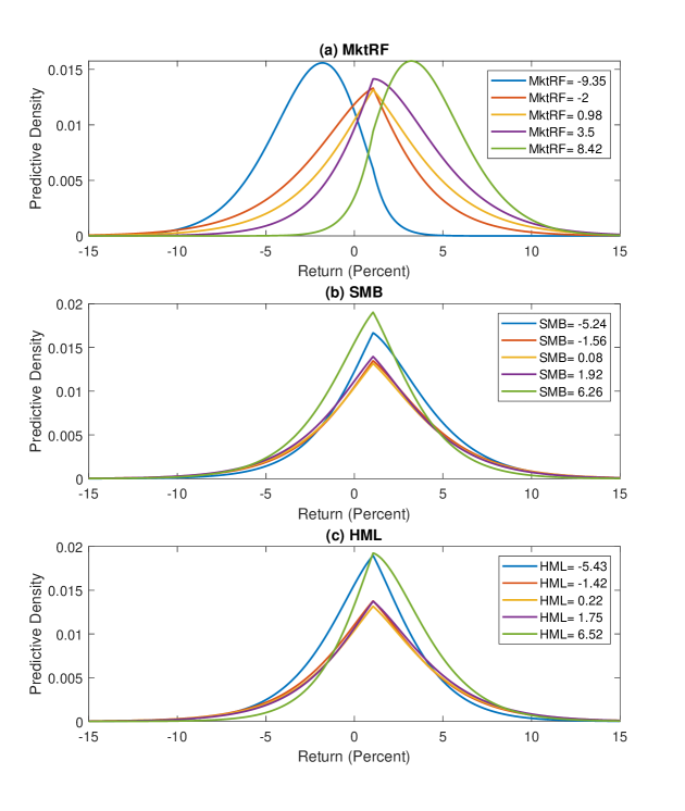
Figure 6: Predictive densities of $Y$ (excess monthly return on AXP, in percent). Panel (a) plots densities for five values of MktRf corresponding to the 0.025, 0.25, 0.5, 0.75 and 0.975 observed quantiles, while setting the remaining covariates to their median values. Panels (b) and (c) repeat the process for covariates SMB and HML, respectively.

6.4 Further reading

Extensions

While there are only $p=5$ covariates in the example here, the regularization provided by the horseshoe prior allows $\text{\boldmath$x$}_{i}$ to be of much higher dimension $p$. In particular, Klein and Smith (2019) suggest forming $\text{\boldmath$x$}_{i}$ using a large number of functional basis terms, such as radial or p-spline bases. This produces a semiparametric distributional regression model that these authors call a “copula smoother”. Klein et al. (2021) instead suggest using the large number of terms from the output layer of a deep neural network (DNN) to form $\text{\boldmath$x$}_{i}$. The result is a “deep distributional regression” method that combines the flexibility of a DNN with the probabilistic calibration of the copula model.

The implicit copula process described in Section 6.3 can also be extended in several directions. Klein and Smith (2020) derive the implicit copula for a linear regression with spike-and-slab priors for $\beta$. This extends popular Bayesian variable selection methods to a dependent variable with an arbitrary marginal distribution. Smith and Klein (2021) extend the homoscedastic regression for the auxiliary response $\tilde{Z}_{i}$ to a heteroscedastic regression. The resulting implicit copula is a mixture of Gaussian copulas, and more flexible than the linear regression copula outlined here. Implicit copula processes constructed from other regression models are also possible.

Other approaches

At (21) the marginals $F_{Y_{j}}$ are assumed independent of the covariates, while the copula is not. In contrast, the copula can be assumed to be independent of the covariates, while the marginals are not; for examples, see Oakes and Ritz (2000), Pitt et al. (2006) and Song et al. (2009). The first approach defines a copula process for a univariate response, whereas the latter approach defines a multivariate regression model for multiple response variables.

The implicit regression copulas outlined in Section 6.2 have a dependence structure that is a parametric function of the covariates through the inversion of Sklar’s theorem. For a linear regression, this is given by the expression for the correlation matrix $R(\text{\boldmath$x$}_{1:N},\text{\boldmath$\theta$})$ at (30). An alternative is to make either the parameters or dependence metrics of a copula $C$ smooth functions of the covariates without directly using inversion. Such models are called “conditional copula models”, and there is a extensive literature dealing with this case; for example, see Gijbels et al. (2011); Veraverbeke et al. (2011); Craiu and Sabeti (2012); Acar et al. (2013); Sabeti et al. (2014); Klein and Kneib (2016) and Vatter and Nagler (2018). Another approach is to treat the covariates as a random vector $\bm{X}$ and model it jointly with $Y$ in a copula model, from which the conditional distribution $Y|\bm{X}=\text{\boldmath$x$}$ can be derived. This approach can be easily extended to multivariate responses, as in Zhao and Genest (2019) who employ an elliptical copula with regularization of the parameter space provided by penalization of the coefficients of $\bm{X}$.

7 Discussion

What is an implicit copula?

While every copula $C$ has one or more implicit representations, it is often infeasible to derive the distribution $F_{Z}$ of the auxiliary variables. Instead, in this paper we consider implicit copulas to be those derived from a given parametric continuous distribution $F_{Z}$. Knowledge of $F_{Z}$ makes estimation of these implicit copulas tractable when using likelihood-based estimation methods, such as Bayesian MCMC or variational inference. This includes high-dimensional cases where $C$ or $c$ cannot be computed in reasonable time, such as the time series and regression copula processes discussed in this paper that have dimension equal to the number of observations.

Comparison with vines

Another copula family that can be employed in high dimensions are vine copulas (Joe, 1996; Bedford and Cooke, 2002). These are constructed from bivariate copula building blocks called “pair-copulas” by Aas et al. (2009). By selecting different pair-copulas, vines can be constructed with a wide range of dependence structures; see Czado (2019) for an overview. Vines are based on a decomposition into conditional distributions. In some applications an appropriate decomposition arises naturally, such as with time series as in Smith et al. (2010), or when conditioning on latent factors as in Krupskii and Joe (2013, 2020). But, in general, there are many different possibilities (Morales-Nápoles et al., 2010) and it can be difficult to select an appropriate choice, although there have been advances in approaches to do so (Czado, 2019). Another challenge in high dimensions is that it can be slow to evaluate the copula density and simulate from the vine, both of which are necessary for parameter estimation and inference. However, truncation as in Brechmann et al. (2012) or other simplifications, such as for stationary Markov time series (Smith et al., 2010; Smith, 2015; Beare and Seo, 2015), can alleviate these problems. In contrast, it is often unnecessary to evaluate the implicit copula density when estimating the copula model, and simulation from high dimensional implicit copulas is typically fast and stable using Algorithm 1.

Discrete and mixed marginals

Copulas with discrete and mixed marginals are very increasingly popular (Genest and Nešlehová, 2007), although parameter estimation is challenging. Several approximate likelihood approaches based on the continuous extension of discrete random variables studied by Denuit and Lambert (2005) have been suggested, although these typically exhibit significant bias in the copula parameter estimates; see Nikoloulopoulos (2013b) and Nikoloulopoulos (2016) for demonstrations using the Gaussian copula. In contrast, Bayesian data augmentation approaches discussed here can evaluate the posterior of such parametric copula models in high dimensions without resorting to approximating the likelihood. For implicit copulas, estimation using data augmentation based on the extended likelihood in Section 2.4 is popular in practice due to its simplicity and robustness. When using MCMC sampling, as in Pitt et al. (2006) for the Gaussian copula, the posterior is evaluated exactly (up to Monte Carlo error) and can be used in high dimensions as demonstrated by Danaher and Smith (2011) and Dobra et al. (2011). An alternative approach that can be used in even higher dimensions is variational inference, as Loaiza-Maya and Smith (2019) outline, although this is an approximate estimation method.

While the Gaussian copula is by far the most popular choice when modeling the dependence of discrete data, it is not clear that it is always the best choice. For example, Smith et al. (2012) found that a skew $t$ copula provided a substantial improvement over a symmetric $t$ copula for 15-dimensional discrete data. While not explored here, implicit copula processes can also be used for discrete time series data. Doing so provides an alternative to the Markov vine copula models currently popular, as in Loaiza-Maya and Smith (2019) and Emura et al. (2021).

Potential of implicit copula processes

Finally, this article aims to highlight the potential of time series and regression implicit copula processes. In machine learning they offer a computationally convenient avenue to extend existing deep models to allow for uncertainty quantification. Examples include Salinas et al. (2019) who do so using Gaussian copula processes and Klein et al. (2020) who using the regression copulas in Section 6 with deep basis functions. The state space copula proposed by Smith and Maneesoonthorn (2018) and outlined in Section 4.3 also has substantial potential. Many existing statistical and econometric models can be written in state space form, from simple time series models to smoothing splines. Combining their implicit copulas with flexible marginals extends these models to more complex data distributions in a straightforward fashion.

Appendix A Evaluation of Marginals

Exact evaluation

When estimating implicit copulas using likelihood-based methods, the marginal quantile functions $F_{Z_{i}}^{-1}$ and the densities $f_{Z_{i}}$ require evaluation. For more complex implicit copulas each distribution function $F_{Z_{i}}(q)=\int_{-\infty}^{q}f_{Z_{i}}(s)\mbox{d}s$ is evaluated using univariate numerical integration. The quantile function can then be obtained using a standard root finding algorithm such as Newton’s method, which typically only requires a small number of steps to obtain an accurate value. This is much faster than using Monte Carlo simulation from $F_{Z_{i}}$.

Fast interpolation

However, for some applications the marginal quantile and density functions of $Z_{i}$ have to be evaluated at many observations. For example, this is the case with time series copulas when $Z_{i}$ has a time invariant margin. To do so quickly the interpolation-based algorithm in Smith and Maneesoonthorn (2018, App. A) can be used, which is fast to compute once the interpolation is complete. These authors show it is accurate for the state space models they study, while Yoshiba (2018) show the same algorithm is also accurate for the margin of a skew $t$ distribution. The algorithm is given below, and it produces approximations for $\log(f_{Z_{i}})$ and $F^{-1}_{Z_{i}}$ far out into the tails of the distribution, which can be used to evaluate the functions quickly at many values.

Algorithm 4 (Interpolation of Quantile and Log-Density at $N$ Points)

• Set $p_{1}=0.0001$ and $p_{N}=0.9999$, and evaluate both $q_{1}=F_{Z_{i}}^{-1}(p_{1})$ and $q_{N}=F_{Z_{i}}^{-1}(p_{N})$ using a root finding algorithm (e.g. Newton’s method).

• Set step size to $\delta=(q_{N}-q_{1})/(N-1)$, and a construct uniform grid as $q_{i}=q_{1}+(i-1)\delta$, for $i=2,\ldots,N$; (e.g. $N=100$ is often sufficient).

• For $i=1,\ldots,N$ (in parallel):

  • Compute $p_{i}=F_{Z_{i}}(q_{i})$ (possibly using univariate numerical integration)

  • Compute $b_{i}=\log(f_{Z_{i}}(q_{i}))$

• Using an interpolation method (e.g. spline interpolation):

  • Interpolate the points $\{(p_{i},q_{i});i=1,\ldots,N\}$ to obtain $F_{Z_{i}}^{-1}$

  • Interpolate the points $\{(q_{i},b_{i});i=1,\ldots,N\}$ to obtain $\log(p_{Z_{i}})$

References

- Aas et al. (2009) Aas, K., Czado, C., Frigessi, A., Bakken, H., 2009. Pair-copula constructions of multiple dependence. Insurance: Mathematics and Economics 44, 182–198.
- Abdous et al. (2005) Abdous, B., Genest, C., Rémillard, B., 2005. Dependence properties of meta-elliptical distributions, in: Duchesne, P., Rémillard, B. (Eds.), Statistical Modeling and Analysis for Complex Data Problems. Springer US, pp. 1–15.
- Acar et al. (2013) Acar, E.F., Craiu, R.V., Yao, F., 2013. Statistical testing of covariate effects in conditional copula models. Electronic Journal of Statistics 7, 2822–2850.
- Ang and Chen (2002) Ang, A., Chen, J., 2002. Asymmetric correlations of equity portfolios. Journal of Financial Economics 63, 443–494.
- Azzalini and Capitanio (2003) Azzalini, A., Capitanio, A., 2003. Distributions generated by perturbation of symmetry with emphasis on a multivariate skew t-distribution. Journal of the Royal Statistical Society: Series B 65, 367–389.
- Azzalini and Dalla Valle (1996) Azzalini, A., Dalla Valle, A., 1996. The multivariate skew-normal distribution. Biometrika 83, 715–726.
- Bai et al. (2014) Bai, Y., Kang, J., Song, P.X.K., 2014. Efficient pairwise composite likelihood estimation for spatial-clustered data. Biometrics 70, 661–670.
- Beare (2010) Beare, B.K., 2010. Copulas and temporal dependence. Econometrica 78, 395–410.
- Beare and Seo (2015) Beare, B.K., Seo, J., 2015. Vine copula specifications for stationary multivariate Markov chains. Journal of Time Series Analysis 36, 228–246.
- Bedford and Cooke (2002) Bedford, T., Cooke, R.M., 2002. Vines: A new graphical model for dependent random variables. Annals of Statistics , 1031–1068.
- Bhat and Eluru (2009) Bhat, C.R., Eluru, N., 2009. A copula-based approach to accommodate residential self-selection effects in travel behavior modeling. Transportation Research Part B: Methodological 43, 749–765.
- Biller and Nelson (2003) Biller, B., Nelson, B.L., 2003. Modeling and generating multivariate time-series input processes using a vector autoregressive technique. ACM Transactions on Modeling and Computer Simulation (TOMACS) 13, 211–237.
- Bitto and Frühwirth-Schnatter (2019) Bitto, A., Frühwirth-Schnatter, S., 2019. Achieving shrinkage in a time-varying parameter model framework. Journal of Econometrics 210, 75–97.
- Bladt and McNeil (2021) Bladt, M., McNeil, A.J., 2021. Time series copula models using d-vines and v-transforms. Econometrics and Statistics In Press.
- Blei et al. (2017) Blei, D.M., Kucukelbir, A., McAuliffe, J.D., 2017. Variational inference: A review for statisticians. Journal of the American statistical Association 112, 859–877.
- Brechmann and Czado (2015) Brechmann, E.C., Czado, C., 2015. Copar—multivariate time series modeling using the copula autoregressive model. Applied Stochastic Models in Business and Industry 31, 495–514.
- Brechmann et al. (2012) Brechmann, E.C., Czado, C., Aas, K., 2012. Truncated regular vines in high dimensions with application to financial data. Canadian Journal of Statistics 40, 68–85.
- Cario and Nelson (1996) Cario, M.C., Nelson, B.L., 1996. Autoregressive to anything: Time-series input processes for simulation. Operations Research Letters 19, 51–58.
- Carvalho and Polson (2010) Carvalho, C.M., Polson, Nicholas, G., 2010. The horseshoe estimator for sparse signals. Biometrika 97, 465–480.
- Chan and Jeliazkov (2009) Chan, J.C., Jeliazkov, I., 2009. Efficient simulation and integrated likelihood estimation in state space models. International Journal of Mathematical Modelling and Numerical Optimisation 1, 101–120.
- Chan and Kroese (2010) Chan, J.C., Kroese, D.P., 2010. Efficient estimation of large portfolio loss probabilities in t-copula models. European Journal of Operational Research 205, 361–367.
- Chen et al. (2012) Chen, Q., Gerlach, R., Lu, Z., 2012. Bayesian Value-at-Risk and expected shortfall forecasting via the asymmetric Laplace distribution. Computational Statistics & Data Analysis 56, 3498–3516.
- Chen and Fan (2006) Chen, X., Fan, Y., 2006. Estimation of copula-based semiparametric time series models. Journal of Econometrics 130, 307–335.
- Cherubini et al. (2004) Cherubini, U., Luciano, E., Vecchiato, W., 2004. Copula methods in finance. John Wiley & Sons.
- Chib and Greenberg (1998) Chib, S., Greenberg, E., 1998. Analysis of multivariate probit models. Biometrika 85, 347–361.
- Clemen and Reilly (1999) Clemen, R.T., Reilly, T., 1999. Correlations and copulas for decision and risk analysis. Management Science 45, 208–224.
- Craiu and Sabeti (2012) Craiu, V.R., Sabeti, A., 2012. In mixed company: Bayesian inference for bivariate conditional copula models with discrete and continuous outcomes. Journal of Multivariate Analysis 110, 106–120.
- Creal and Tsay (2015) Creal, D.D., Tsay, R.S., 2015. High dimensional dynamic stochastic copula models. Journal of Econometrics 189, 335–345.
- Czado (2019) Czado, C., 2019. Analyzing dependent data with vine copulas. Lecture Notes in Statistics, Springer .
- Danaher and Smith (2011) Danaher, P.J., Smith, M.S., 2011. Modeling multivariate distributions using copulas: Applications in marketing. Marketing Science 30, 4–21.
- Darsow et al. (1992) Darsow, W.F., Nguyen, B., Olsen, E.T., et al., 1992. Copulas and Markov processes. Illinois Journal of Mathematics 36, 600–642.
- Deheuvels (1979) Deheuvels, P., 1979. La fonction de dépendance empirique et ses propriétés. un test non paramétrique d’indépendance. Bulletins de l’Académie Royale de Belgique 65, 274–292.
- Demarta and McNeil (2005) Demarta, S., McNeil, A.J., 2005. The t copula and related copulas. International Statistical Review 73, 111–129.
- Denuit and Lambert (2005) Denuit, M., Lambert, P., 2005. Constraints on concordance measures in bivariate discrete data. Journal of Multivariate Analysis 93, 40–57.
- Dobra et al. (2011) Dobra, A., Lenkoski, A., et al., 2011. Copula Gaussian graphical models and their application to modeling functional disability data. The Annals of Applied Statistics 5, 969–993.
- Durante and Sempi (2015) Durante, F., Sempi, C., 2015. Principles of copula theory. CRC press.
- Durbin and Koopman (2012) Durbin, J., Koopman, S.J., 2012. Time series analysis by state space methods. Oxford University Press.
- Embrechts et al. (2002) Embrechts, P., McNeil, A., Straumann, D., 2002. Correlation and dependence in risk management: Properties and pitfalls, in: Dempster, M.A.H. (Ed.), Risk Management: Value at Risk and Beyond. Cambridge University Press, pp. 176–223.
- Emura et al. (2021) Emura, T., Lai, C.C., Sun, L.H., 2021. Change point estimation under a copula-based markov chain model for binomial time series. Econometrics and Statistics In Press.
- Fama and French (2015) Fama, E.F., French, K.R., 2015. A five-factor asset pricing model. Journal of Financial Economics 116, 1–22.
- Fang et al. (2002) Fang, H.B., Fang, K.T., Kotz, S., 2002. The meta-elliptical distributions with given marginals. Journal of Multivariate Analysis 82, 1–16.
- Favre et al. (2004) Favre, A.C., El Adlouni, S., Perreault, L., Thiémonge, N., Bobée, B., 2004. Multivariate hydrological frequency analysis using copulas. Water Resources Research 40.
- Frees and Valdez (1998) Frees, E.W., Valdez, E.A., 1998. Understanding relationships using copulas. North American Actuarial Journal 2, 1–25.
- Frees and Wang (2005) Frees, E.W., Wang, P., 2005. Credibility using copulas. North American Actuarial Journal 9, 31–48.
- Frees and Wang (2006) Frees, E.W., Wang, P., 2006. Copula credibility for aggregate loss models. Insurance: Mathematics and Economics 38, 360 – 373.
- Frühwirth-Schnatter and Lopes (2018) Frühwirth-Schnatter, S., Lopes, H.F., 2018. Sparse Bayesian factor analysis when the number of factors is unknown. arXiv preprint arXiv:1804.04231 .
- Genest et al. (2007) Genest, C., Favre, A.C., Béliveau, J., Jacques, C., 2007. Metaelliptical copulas and their use in frequency analysis of multivariate hydrological data. Water Resources Research 43.
- Genest and MacKay (1986) Genest, C., MacKay, J., 1986. The joy of copulas: bivariate distributions with uniform marginals. The American Statistician 40, 280–283.
- Genest and Nešlehová (2007) Genest, C., Nešlehová, J., 2007. A primer on copulas for count data. ASTIN Bulletin: The Journal of the IAA 37, 475–515.
- Genton (2004) Genton, M.G., 2004. Skew-elliptical distributions and their applications: a journey beyond normality. CRC Press.
- Gijbels et al. (2011) Gijbels, I., Veraverbeke, N., Omelka, M., 2011. Conditional copulas, association measures and their applications. Computational Statistics & Data Analysis 55, 1919–1932.
- Gunawan et al. (2020) Gunawan, D., Khaled, M.A., Kohn, R., 2020. Mixed marginal copula modeling. Journal of Business & Economic Statistics 38, 137–147.
- Hafner and Manner (2012) Hafner, C.M., Manner, H., 2012. Dynamic stochastic copula models: Estimation, inference and applications. Journal of Applied Econometrics 27, 269–295.
- Hoff et al. (2007) Hoff, P.D., et al., 2007. Extending the rank likelihood for semiparametric copula estimation. The Annals of Applied Statistics 1, 265–283.
- Huber et al. (2020) Huber, F., Koop, G., Onorante, L., 2020. Inducing sparsity and shrinkage in time-varying parameter models. Journal of Business and Economic Statistics Forthcoming.
- Hughes (2015) Hughes, J., 2015. copCAR: A flexible regression model for areal data. Journal of Computational and Graphical Statistics 24, 733–755.
- Ibragimov (2009) Ibragimov, R., 2009. Copula-based characterizations for higher order Markov processes. Econometric Theory 25, 819–846.
- Jaworski et al. (2010) Jaworski, P., Durante, F., Hardle, W.K., Rychlik, T., 2010. Copula theory and its applications. volume 198. Springer.
- Joe (1993) Joe, H., 1993. Parametric families of multivariate distributions with given margins. Journal of Multivariate Analysis 46, 262–282.
- Joe (1996) Joe, H., 1996. Families of m-variate distributions with given margins and m(m-1)/2 bivariate dependence parameters. Lecture Notes-Monograph Series , 120–141.
- Joe (1997) Joe, H., 1997. Multivariate models and dependence concepts. Chapman & Hall.
- Joe (2005) Joe, H., 2005. Asymptotic efficiency of the two-stage estimation method for copula-based models. Journal of Multivariate Analysis 94, 401–419.
- Joe (2014) Joe, H., 2014. Dependence modeling with copulas. CRC press.
- Kaufmann and Schumacher (2017) Kaufmann, S., Schumacher, C., 2017. Identifying relevant and irrelevant variables in sparse factor models. Journal of Applied Econometrics 32, 1123–1144.
- Klein and Kneib (2016) Klein, N., Kneib, T., 2016. Simultaneous inference in structured additive conditional copula regression models: a unifying Bayesian approach. Statistics and Computing 26, 841–860.
- Klein et al. (2015) Klein, N., Kneib, T., Lang, S., 2015. Bayesian generalized additive models for location, scale, and shape for zero-inflated and overdispersed count data. Journal of the American Statistical Association 110, 405–419.
- Klein et al. (2021) Klein, N., Nott, D.J., Smith, M.S., 2021. Marginally calibrated deep distributional regression. Journal of Computational and Graphical Statistics 30, 467–483.
- Klein and Smith (2019) Klein, N., Smith, M.S., 2019. Implicit copulas from Bayesian regularized regression smoothers. Bayesian Analysis 14, 1143–1171.
- Klein and Smith (2020) Klein, N., Smith, M.S., 2020. Bayesian variable selection for non-gaussian responses: a marginally calibrated copula approach. Biometrics Forthcoming.
- Klein et al. (2020) Klein, N., Smith, M.S., Nott, D.J., 2020. Deep distributional time series models and the probabilistic forecasting of intraday electricity prices. arXiv preprint arXiv:2010.01844 .
- Kneib et al. (2021) Kneib, T., Silbersdorff, A., Säfken, B., 2021. Rage against the mean – a review of distributional regression approaches. Econometrics and Statistics In Press.
- Krupskii and Joe (2013) Krupskii, P., Joe, H., 2013. Factor copula models for multivariate data. Journal of Multivariate Analysis 120, 85–101.
- Krupskii and Joe (2020) Krupskii, P., Joe, H., 2020. Flexible copula models with dynamic dependence and application to financial data. Econometrics and Statistics 16, 148–167.
- Lambert and Vandenhende (2002) Lambert, P., Vandenhende, F., 2002. A copula-based model for multivariate non-normal longitudinal data: analysis of a dose titration safety study on a new antidepressant. Statistics in Medicine 21, 3197–3217.
- Laurent and Gregory (2005) Laurent, J.P., Gregory, J., 2005. Basket default swaps, cdos and factor copulas. Journal of Risk 7, 103–122.
- Li (2000) Li, D.X., 2000. On default correlation: A copula function approach. The Journal of Fixed Income 9, 43–54.
- Li and Hammond (1975) Li, S.T., Hammond, J.L., 1975. Generation of pseudorandom numbers with specified univariate distributions and correlation coefficients. IEEE Transactions on Systems, Man, and Cybernetics SMC-5, 557–561.
- Loaiza-Maya and Smith (2019) Loaiza-Maya, R., Smith, M.S., 2019. Variational Bayes estimation of discrete-margined copula models with application to time series. Journal of Computational and Graphical Statistics 28, 523–539.
- Loaiza-Maya et al. (2018) Loaiza-Maya, R., Smith, M.S., Maneesoonthorn, W., 2018. Time series copulas for heteroskedastic data. Journal of Applied Econometrics 33, 332–354.
- Longin and Solnik (2001) Longin, F., Solnik, B., 2001. Extreme correlation of international equity markets. The Journal of Finance 56, 649–676.
- Lütkepohl (2005) Lütkepohl, H., 2005. New introduction to multiple time series analysis. Springer Science & Business Media.
- Masarotto et al. (2012) Masarotto, G., Varin, C., et al., 2012. Gaussian copula marginal regression. Electronic Journal of Statistics 6, 1517–1549.
- Mazo et al. (2016) Mazo, G., Girard, S., Forbes, F., 2016. A flexible and tractable class of one-factor copulas. Statistics and Computing 26, 965–979.
- McNeil et al. (2005) McNeil, A.J., Frey, R., Embrechts, R., 2005. Quantitative Risk Management: Concepts, Techniques and Tools. Princeton University Pres, Princton: NJ.
- Morales-Nápoles et al. (2010) Morales-Nápoles, O., Cooke, R.M., Kurowicka, D., 2010. About the number of vines and regular vines on nodes. Technical Report. Delft University of Technology.
- Murray et al. (2013) Murray, J.S., Dunson, D.B., Carin, L., Lucas, J.E., 2013. Bayesian Gaussian copula factor models for mixed data. Journal of the American Statistical Association 108, 656–665.
- Nagler et al. (2020) Nagler, T., Krüger, D., Min, A., 2020. Stationary vine copula models for multivariate time series. arXiv preprint arXiv:2008.05990 .
- Nelsen (2006) Nelsen, R.B., 2006. An Introduction to Copulas. Springer-Verlag, New York, Secaucus, NJ, USA.
- Nikoloulopoulos (2013a) Nikoloulopoulos, A.K., 2013a. Copula-based models for multivariate discrete response data, in: Copulae in Mathematical and Quantitative Finance. Springer, pp. 231–249.
- Nikoloulopoulos (2013b) Nikoloulopoulos, A.K., 2013b. On the estimation of normal copula discrete regression models using the continuous extension and simulated likelihood. Journal of Statistical Planning and Inference 143, 1923–1937.
- Nikoloulopoulos (2016) Nikoloulopoulos, A.K., 2016. Efficient estimation of high-dimensional multivariate normal copula models with discrete spatial responses. Stochastic environmental research and risk assessment 30, 493–505.
- Nikoloulopoulos and Joe (2015) Nikoloulopoulos, A.K., Joe, H., 2015. Factor copula models for item response data. Psychometrika 80, 126–150.
- Oakes and Ritz (2000) Oakes, D., Ritz, J., 2000. Regression in a bivariate copula model. Biometrika 87, 345–352.
- Oh and Patton (2017) Oh, D.H., Patton, A.J., 2017. Modeling dependence in high dimensions with factor copulas. Journal of Business & Economic Statistics 35, 139–154.
- Oh and Patton (2018) Oh, D.H., Patton, A.J., 2018. Time-varying systemic risk: Evidence from a dynamic copula model of CDS spreads. Journal of Business & Economic Statistics 36, 181–195.
- Oh and Patton (2020) Oh, D.H., Patton, A.J., 2020. Dynamic factor copula models with estimated cluster assignments. Available at SSRN 3724645 .
- Opschoor et al. (2020) Opschoor, A., Lucas, A., Barra, I., Van Dijk, D., 2020. Closed-form multi-factor copula models with observation-driven dynamic factor loadings. Journal of Business & Economic Statistics , 1–38.
- Park and Gupta (2012) Park, S., Gupta, S., 2012. Handling endogenous regressors by joint estimation using copulas. Marketing Science 31, 567–586.
- Patton (2006) Patton, A.J., 2006. Modelling asymmetric exchange rate dependence. International Economic Review 47, 527–556.
- Patton (2012) Patton, A.J., 2012. A review of copula models for economic time series. Journal of Multivariate Analysis 110, 4–18.
- Pitt et al. (2006) Pitt, M., Chan, D., Kohn, R., 2006. Efficient Bayesian inference for Gaussian copula regression models. Biometrika 93, 537–554.
- Polson and Scott (2012) Polson, N.G., Scott, J.G., 2012. On the half-Cauchy prior for a global scale parameter. Bayesian Analysis 7, 887–902.
- Rémillard et al. (2012) Rémillard, B., Papageorgiou, N., Soustra, F., 2012. Copula-based semiparametric models for multivariate time series. Journal of Multivariate Analysis 110, 30–42.
- Rodriguez (2007) Rodriguez, J.C., 2007. Measuring financial contagion: A copula approach. Journal of Empirical Finance 14, 401–423.
- Rüschendorf (1976) Rüschendorf, L., 1976. Asymptotic distributions of multivariate rank order statistics. The Annals of Statistics 4, 912–923.
- Rüschendorf (2009) Rüschendorf, L., 2009. On the distributional transform, sklar’s theorem, and the empirical copula process. Journal of Statistical Planning and Inference 139, 3921–3927.
- Sabeti et al. (2014) Sabeti, A., Wei, M., Craiu, R.V., 2014. Additive models for conditional copulas. Stat 3, 300–312.
- Sahu et al. (2003) Sahu, S.K., Dey, D.K., Branco, M.D., 2003. A new class of multivariate skew distributions with applications to Bayesian regression models. Canadian Journal of Statistics 31, 129–150.
- Salinas et al. (2019) Salinas, D., Bohlke-Schneider, M., Callot, L., Medico, R., Gasthaus, J., 2019. High-dimensional multivariate forecasting with low-rank Gaussian copula processes, in: Advances in Neural Information Processing Systems, pp. 6827–6837.
- Schamberger et al. (2017) Schamberger, B., Gruber, L.F., Czado, C., 2017. Bayesian inference for latent factor copulas and application to financial risk forecasting. Econometrics 5, 21.
- Schoelzel and Friederichs (2008) Schoelzel, C., Friederichs, P., 2008. Multivariate non-normally distributed random variables in climate research–introduction to the copula approach. Nonlinear Processes in Geophysics 15, 761–772.
- Shimazaki and Shinomoto (2010) Shimazaki, H., Shinomoto, S., 2010. Kernel bandwidth optimization in spike rate estimation. Jorunal of Computational Neuroscience 29, 171–182.
- Sklar (1959) Sklar, A., 1959. Fonctions de repartition a n dimensions et leur marges. Publ. Inst. Statist. Univ. Paris 8, 229231 8, 229–231.
- Smith et al. (2010) Smith, M., Min, A., Almeida, C., Czado, C., 2010. Modeling longitudinal data using a pair-copula decomposition of serial dependence. Journal of the American Statistical Association 105, 1467–1479.
- Smith (2013) Smith, M.S., 2013. Bayesian approaches to copula modelling, in: Damien, P., Dellaportas, P., Polson, N.G., Stephens, D.A. (Eds.), Bayesian Theory and Applications. Oxford University Press, pp. 336–358.
- Smith (2015) Smith, M.S., 2015. Copula modelling of dependence in multivariate time series. International Journal of Forecasting 31, 815–833.
- Smith et al. (2012) Smith, M.S., Gan, Q., Kohn, R.J., 2012. Modelling dependence using skew t copulas: Bayesian inference and applications. Journal of Applied Econometrics 27, 500–522.
- Smith and Kauermann (2011) Smith, M.S., Kauermann, G., 2011. Bicycle commuting in Melbourne during the 2000s energy crisis: A semiparametric analysis of intraday volumes. Transportation Research, Part B: Methodological 45, 1846–1862.
- Smith and Khaled (2012) Smith, M.S., Khaled, M.A., 2012. Estimation of copula models with discrete margins via Bayesian data augmentation. Journal of the American Statistical Association 107, 290–303.
- Smith and Klein (2021) Smith, M.S., Klein, N., 2021. Bayesian inference for regression copulas. Journal of Business & Economic Statistics 39, 712–728.