In-orbit timing calibration of Insight-Hard X-ray Modulation Telescope

Abstract

We describe the timing system and the timing calibration results of the three payloads on-board the Insight-Hard X-ray Modulation Telescope (Insight-HXMT). These three payloads are the High Energy X-ray telescope (HE, 20-250 keV), the Medium Energy X-ray telescope (ME, 5-30 keV) and the low Energy X-ray telescope (LE, 1-10 keV). We present a method to correct the temperature-dependent period response and the long-term variation of the on-board crystal oscillator, especially for ME that does not carry a temperature-compensated crystal oscillator. The time of arrivals (ToAs) of the Crab pulsar are measured to evaluate the accuracy of the timing system. As the ephemeris of the Crab pulsar given by Jodrell Bank observatory has systematic errors around (Rots et al., 2004) $40\text{\,}\mathrm{\SIUnitSymbolMicro s}$, we use the quasi-simultaneous observations of the X-ray Timing Instrument (XTI) on-board the Neutron star Interior Composition Explorer (NICER) to produce the Crab ephemerides and to verify the timing system of Insight-HXMT. The energy-dependent ToAs’ offsets relative to the NICER measurements including physical and instrumental origins are about $24.7\text{\,}\mathrm{\SIUnitSymbolMicro s}$, $10.1\text{\,}\mathrm{\SIUnitSymbolMicro s}$ and $864.7\text{\,}\mathrm{\SIUnitSymbolMicro s}$, and the systematic errors of the timing system are determined as $12.1\text{\,}\mathrm{\SIUnitSymbolMicro s}$, $8.6\text{\,}\mathrm{\SIUnitSymbolMicro s}$, and $15.8\text{\,}\mathrm{\SIUnitSymbolMicro s}$, for HE, ME and LE respectively.

1 Introduction

The Hard X-ray Modulation Telescope, dubbed as Insight-HXMT, was successfully launched on June 15th, 2017 into a low earth orbit with an altitude of 550 km and an inclination of 43 degrees (Zhang et al., 2020; Lu & Zhang, 2018; Li et al., 2020). There are three payloads on-board Insight-HXMT, the High Energy X-ray telescope (HE) that contains 18 NaI(Tl)/CsI(Na) phoswich scintillation detectors for observations in 20–250 keV (Liu et al., 2020), the Medium Energy X-ray telescope (ME) with 1728 Si-PIN detectors for 5–30 keV (Cao et al., 2020), and the Low Energy X-ray telescope (LE) with 96 SCD detectors for 1–15 keV (Chen et al., 2020).

Fast X-ray timing observation of astrophysical objects is one of the key capabilities and tasks of Insight-HXMT. High timing accuracy is essential to achieve the scientific goals involving rapid variability, such as rotation and accretion-powered millisecond pulsars, gamma ray bursts and kHz quasi-periodic oscillations. This is the reason that Insight-HXMT carries a GPS receiver (GPSR) on-board. The high precision of the Insight-HXMT timing system was at least partly demonstrated in the experiments of autonomous space navigation with pulsars (Zheng et al., 2019), but an exact calibration has not yet been performed. In this paper, the main purpose is to perform an in-orbit timing calibration for Insight-HXMT. Most missions in X-ray and Gamma-ray perform in-orbit timing calibration by observing pulsars, especially millisecond pulsars, which have stable timing properties. However, millisecond pulsars are very faint for Insight-HXMT due to its high background level (Liao et al., 2020a; Guo et al., 2020; Liao et al., 2020b) and thus the Crab pulsar is the most suitable source for timing calibration of Insight-HXMT.

Actually the timing calibrations of some other X-ray or Gamma-ray telescopes are also carried out based on the observations of the Crab pulsar. The timing calibration, based on the Crab pulsar in X-ray and Gamma-ray bands, typically measures the delay of the radio main pulse of the Crab pulsar compared to the main pulse observed by the respective satellite. Enoto et al. (2021) measured the difference between Crab’s X-ray and radio pulse profiles and radio observations (using radio telescopes at Usuda and Kashima), and found that the main pulse ahead of radio main pulse and deviation of NICER are about $304\text{\,}\mathrm{\SIUnitSymbolMicro s}$ and $1.3\text{\,}\mathrm{\SIUnitSymbolMicro s}$; the main pulse observed by Suzaku/HXD precedes RXTE/PCA, RXTE/HEXTE, INTEGRAL/IBIS ISGRI, and Swift/BAT by $0.003\pm 0.001$, $0.002\pm 0.001$, $0.002\pm 0.001$, $0.002\pm 0.001$ periods, respectively (Terada et al., 2008). Thus the offset of Suzaku/HXD leads those X-ray instruments by about $70\text{\,}\mathrm{\SIUnitSymbolMicro s}$, and the systematic error is $270\text{\,}\mathrm{\SIUnitSymbolMicro s}$ obtained by Jodrell Bank ephemeris. The following instruments verify the offsets and systematic errors based on the ephemerides given by Jodrell Bank observatory as well. RXTE/PCA’s offset to radio Jodrell Bank observation is $344\text{\,}\mathrm{\SIUnitSymbolMicro s}$ and systematic error is $40\text{\,}\mathrm{\SIUnitSymbolMicro s}$ (Rots et al., 2004); INTEGRAL/SPI offers offset of $280\text{\,}\mathrm{\SIUnitSymbolMicro s}$ and systematic error of $40\text{\,}\mathrm{\SIUnitSymbolMicro s}$ (Kuiper et al., 2003; Molkov et al., 2010); Fermi/GBM’s offset is $222\pm 4$ $\mathrm{\SIUnitSymbolMicro s}$ and systematic error is $56\text{\,}\mathrm{\SIUnitSymbolMicro s}$, while Fermi/LAT’s offset is $111\pm 4$ $\mathrm{\SIUnitSymbolMicro s}$ and systematic error of $57\text{\,}\mathrm{\SIUnitSymbolMicro s}$ (Aliu et al., 2011), and all results are epoch-folded by Jodrell Bank ephemeris. For RXTE/PCA and INTEGRAL/SPI, the systematic error obtained by Jodrell Bank ephemeris is mainly caused by the interstellar scattering and instrument calibration of the radio telescope (Rots et al., 2004). Therefore, we decide to utilize the observations of NICER to produce the Crab ephemeris and to estimate the offset and systematic error of Insight-HXMT in the quasi-simultaneous time intervals.

In this paper, we give a description of the timing system of Insight-HXMT. The detailed time assignment procedure and the correction on the period of crystal oscillator are presented in Section 2. In section 3, we describe our measurements, data processing and timing analysis method on the Crab pulsar observations. In section 4, the Crab ephemeris are derived by NICER/XTI observations. The offsets relative to NICER/XTI measurements and the systematic errors of Insight-HXMT timing system are presented by the ephemerides. The Section 5 summarizes our results.

2 The timing system of Insight-HXMT

Insight-HXMT satellite carries a GPSR to obtain accurate time information from GPS satellites and distributes the GPS pulse per second (PPS) to each payload. After about 250 ms, the mission elapsed time (MET) for the GPS pulse, relative to 2012-01-01T00:00:00 (UTC), is also sent to each payload. The GPS pulse and MET time are stored as a pair in the raw data package of each payload. If the GPS fails or is locked off, an alternative module in GPSR will generate PPS.

Insight-HXMT also carries a high-stability time unit (HSTU) with a frequency of 5 MHz and stability of $3\times 10^{-8}\,\rm{s}^{-1}$. The clock distributor in the HE and LE payloads use this 5 MHz to generate $2\text{\,}\mathrm{\SIUnitSymbolMicro s}$ and $1\text{\,}\mathrm{\SIUnitSymbolMicro s}$ local clock for the data processing unit (DPU), which mean that the time of the HE events is in units of $2\text{\,}\mathrm{\SIUnitSymbolMicro s}$ and the LE events $1\text{\,}\mathrm{\SIUnitSymbolMicro s}$. ME carries an internal quartz oscillator to generate the $6\text{\,}\mathrm{\SIUnitSymbolMicro s}$ local clock by itself. Figure 1 shows a schematic diagram of the timing system of Insight-HXMT.

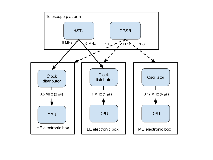
Figure 1: The schematic diagram of the timing system of Insight-HXMT. GPS receiver (GPSR) sends GPS pulse per second (PPS) to the electronic boxes of the three payloads. The high-stability time unit (HSTU) on the platform distributes 5 MHz clocks to HE and LE. The clock distributor in HE uses the 5 MHz clocks to generate local clock with period of $2\text{\,}\mathrm{\SIUnitSymbolMicro s}$ for the data processing unit (DPU) of HE. The clock distributor in LE also utilizes the 5 MHz clock to generate the local clock with period of $1\text{\,}\mathrm{\SIUnitSymbolMicro s}$ and sends to DPU. ME uses a quartz oscillator instead to generate $6\text{\,}\mathrm{\SIUnitSymbolMicro s}$ clock to DPU.

2.1 Time assignment of Insight-HXMT events

In this subsection, we take HE as an example to show the time assignment of the physical events recorded by Insight-HXMT. The timing information of HE events is divided into two parts, one is the integral part of the second (defined as Stime hereafter) and the other is the fractional part of the second (defined as Ptime hereafter). Stime is produced using the GPS pulse provided by GPSR, which is inserted into the physical data stream per second with a special tag. Ptime is the local time count of the $2\text{\,}\mathrm{\SIUnitSymbolMicro s}$ clock cycle. In the raw package of HE, Stime has 32 bits and is increased by one once HE receives the GPS pulse. Therefore, Stime covers time ranges from zero to about 136 years ($2^{32}\,\rm{s}$) if the payload is not turned off and restarted. Ptime has 19 bits and records the local count of clock with cycles of $2\text{\,}\mathrm{\SIUnitSymbolMicro s}$. As a result, Ptime counter will overflow and re-count from zero about every $1.048\text{\,}\mathrm{s}$ ($2^{19}\times$$2\text{\,}\mathrm{\SIUnitSymbolMicro s}$).

In order to compress the amount of ME and LE data, only the lowest 14 bits of Ptime are recorded for each event in ME. A carry-up event is generated when the Ptime counter overflows and resets to zero about every 0.098s ($2^{14}\times$$6\text{\,}\mathrm{\SIUnitSymbolMicro s}$). The number of the carry-up event is recorded in the raw data with 32 bits length. LE also records the lowest 16 bits of Ptime for each event, and a carry-up event is also generated when the Ptime counter overflows and recounts from zero about every 0.065s ($2^{16}\times$$1\text{\,}\mathrm{\SIUnitSymbolMicro s}$). The number of the carry-up event is also recorded in the raw data with 32 bits length. As listed in Table 1, the local time counters of Ptime are summarized for the three payloads on-board Insight-HXMT. The period of the local clock is also the time resolution of the three payloads.

Table 1: The local time counters of Ptime for Insight-HXMT payloads.

Payloads	Bit length	Period of the local clock
HE	19 bits	$2\text{\,}\mathrm{\SIUnitSymbolMicro s}$
ME	14 bits	$6\text{\,}\mathrm{\SIUnitSymbolMicro s}$
LE	16 bits	$1\text{\,}\mathrm{\SIUnitSymbolMicro s}$

The arrival times of X-ray photons from astronomical objects and particles from background are recorded by Ptime only. The GPS pulses are recorded by Stime and Ptime simultaneously as displayed in Figure 2. The physical events are filled between GPS events, and the rate of physical events is decided by the intensities of the astronomical objects and background. Since HSTU is not synchronized to GPSR on-board, the local clock should be corrected by GPS pulses with offline software.

Figure 2: The time assignment of Insight-HXMT/HE events. GPS events recorded by Stime and Ptime are shown with big solid circle and inserted into the event stream every second. The physical events with small solid circle are only recorded by Ptime. Ptime accumulates to $2^{19}$ and starts counting from zero.

2.2 Correction of the arrival times of events

We use an automated data production software to decode the data in the raw package and save the data files in the flexible image transport system (FITS) format. The decoding process calculates the physical values, such as time, pulse height, pulse width, and writes them to the output FITS files.

The temperature-dependent and long-term variation effects on the period of the local clock are corrected by synchronizing Ptime and PPS. In each hour, the Stime of the first GPS pulse can be labeled as $S_{0}$. The nominal local period is $2\text{\,}\mathrm{\SIUnitSymbolMicro s}$ for Ptime, but there may exist jitters. Therefore, the actual period, first and second order derivative of the period in each hour are represented by $\tau$, $\dot{\tau}$ and $\ddot{\tau}$, respectively. The Stime of the GPS pulse, labeled as $S$, increases by one per second and can be modeled as the following Taylor expansion,

$$S=S_{0}+\tau(N-N_{0})+\frac{1}{2}\dot{\tau}(N-N_{0})^{2}+\frac{1}{6}\ddot{\tau}(N-N_{0})^{3}+...,$$ (1)

where $N_{0}$ is the Ptime of the first GPS pulse in each hour, and $N$ is the accumulated local time counts of Ptime in reference to $N_{0}$. The least square fit method is used to obtain the values of $S_{0}$, $\tau$, $\dot{\tau}$ and $\ddot{\tau}$. Then $S$ of the physical events can be derived from Equation (1) according to the accumulated local time counts $N$ in reference to $N_{0}$ and the best fit parameters $S_{0}$, $\tau$, $\dot{\tau}$, $\ddot{\tau}$.

Since each GPS pulse corresponds to an MET time (labeled as $M$), so the MET time of events can be derived as,

$$M=M_{0}+S-S_{0},$$ (2)

where $M_{0}$ represents the MET time of the first GPS pulse in each hour. Then the MET time of an event can be converted into the terrestrial time (TT) value, which is the conventional time system used in the FITS file in X-ray astronomy.

We examined the reliability and accuracy of the time assignment process both before and after the launch. We found that $\tau$ and $\dot{\tau}$ are enough to describe $S$ for HE and LE. But for ME, $\ddot{\tau}$, and $\dddot{\tau}$ should be also included to describe the $S$. The nominal period ($\tau_{0}$) of the three payloads are $2\text{\,}\mathrm{\SIUnitSymbolMicro s}$, $6\text{\,}\mathrm{\SIUnitSymbolMicro s}$, and $1\text{\,}\mathrm{\SIUnitSymbolMicro s}$ for HE, ME, and LE respectively. The relative change ($R$) of $\tau$ can be described as,

$$R=\frac{\tau-\tau_{0}}{\tau_{0}},$$ (3)

In Figure 3, the evolution trends of $R$ for HE and LE are shown respectively. HE and LE both use HSTU provided by the satellite, so the evolution is almost the same.

Figure 4 shows the evolution of $R$ and temperatures measured by ME, and Figure 4 shows the correlation of $R$ and temperature. The period of the quartz oscillator depends largely on the temperature so they have a strong positive correlation. In other words, the effects of temperature variation on the quartz oscillator can be described well by Equation (1). As a result, using this method we can calibrate and correct the long-term variation of the period of the ME quartz oscillator and HSTU. Since ME uses the quartz oscillator carried by itself and the quartz oscillator is not temperature compensated, the relative change of the period supplied by this oscillator is three orders of magnitude higher than HSTU used by HE and LE.

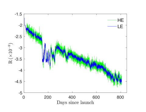
Figure 3: The evolution trends of the relative change of the nominal period for HE and LE. The blue line represents the result of LE and the green line represents the result of HE. Reasons for the deviations from the long time trend around day 200 are yet unknown.

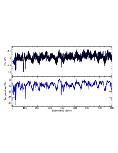
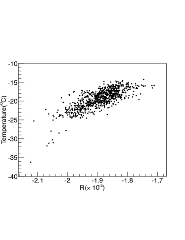
Figure 4: (a) The top panel shows the evolution of the relative change of the nominal period for ME. The bottom panel shows the temperature versus days after launch. The real period of the quartz oscillation depends largely on temperature. (b) The correlation between temperature and relative change of the nominal period $R$.

2.3 The stability of the local clock

After the correction mentioned above, the stability of the local clock is revealed by the residuals between the recorded Stime of the GPS pulse and $S$ calculated by Equation (1).We subtract Stime of the GPS pulse from the arrival time calculated by Equation (1). Their differences of HE and LE in one hour are shown in Figure 5. $S_{0}$, $\tau$ and $\dot{\tau}$ are used for HE and LE. The accuracy of the arrival time of GPS pulse is less than one period of the local clock for HE and LE.

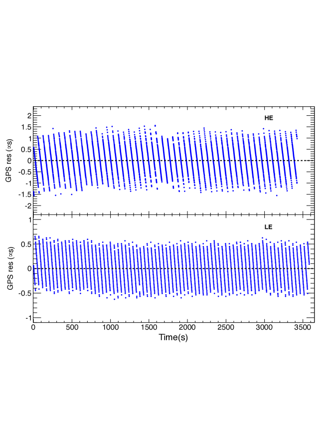
Figure 5: The residuals between the arrival time of GPS pulse in one hour calculated by Equation (1) and Stime which is an integer in seconds. The top panel shows the residual for HE, and the residual is less than $2\text{\,}\mathrm{\SIUnitSymbolMicro s}$ which is the period of the local clock. The bottom panel shows the residual for LE, and the residual is less than $1\text{\,}\mathrm{\SIUnitSymbolMicro s}$ which is the period of the local clock. The slope of each truncated line in each panel refers to the $R$ in Figure 3.

The differences between the arrival time of the GPS pulse calculated by Equation (1) and Stime recorded by ME are plotted in Figure 6, in which panel (a) shows the results in one hour when only terms related to $S_{0}$, $\tau$ and $\dot{\tau}$ are used in Equation (1). Panel (b) shows the results in one hour when we use $S_{0}$, $\tau$, $\dot{\tau}$, and $\ddot{\tau}$ in Equation (1). Panel (c) shows the results in one hour when $S_{0}$ ,$\tau$, $\dot{\tau}$, $\ddot{\tau}$ and $\dddot{\tau}$ are used in Equation (1). Obviously, the third order derivative of $\tau$ is needed to describe the period of local clock and make the arrival time of GPS pulse in less than one period of the local clock for ME.

The stability of the local clock after the correction are within $\pm$$1\text{\,}\mathrm{\SIUnitSymbolMicro s}$, $\pm$$3\text{\,}\mathrm{\SIUnitSymbolMicro s}$, and $\pm$$0.5\text{\,}\mathrm{\SIUnitSymbolMicro s}$ for HE, ME, and LE, respectively. We can then further confirm the performance of the timing system with the observations of the Crab pulsar.

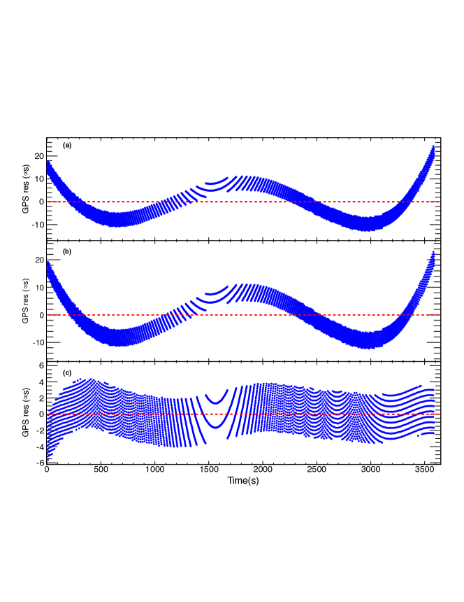
Figure 6: The residuals between the arrival time of GPS pulse in one hour calculated by Equation (1) and Stime for ME. Panel (a) shows the residual using $S_{0}$, $\tau$ and $\dot{\tau}$. Panel (b) shows the residual using $S_{0}$ ,$\tau$ , $\dot{\tau}$ and $\ddot{\tau}$. Panel (c) shows the residual using $S_{0}$ ,$\tau$ ,$\dot{\tau}$, $\ddot{\tau}$ and $\dddot{\tau}$.

3 Observations of the Crab pulsar and data analysis

3.1 Data reduction

The standard data reduction threads are performed using the analysis software HXMTDASv2.04. The recommended criteria for generating the good time intervals (GTIs) are the intervals when (1) elevation angle > 10 degrees; (2) geomagnetic cut-off rigidities > 8 GeV; (3) satellite not in SAA and 300 seconds intervals near SAA; (4) pointing deviation to the source less than 0.04 degree. The Crab is the main calibration target for Insight-HXMT, which conducted a long-term monitoring program with a total effective exposure of $\sim 777\,\rm{ks}$ (78 times of observations until 2020-02-21). Observations with quasi-simultaneous ones by NICER are listed in table 2.

HXMT-Obs_ID	Start (UTC)	Stop (UTC)	NICER-Obs_ID	Start (UTC)	Stop (UTC)
P0111605001	2017-11-09T04:03:40	2017-11-10T00:55:03	ni1013010109	2017-11-09T10:17:39	2017-11-09T10:21:25
P0111605002	2017-11-10T16:39:27	2017-11-11T00:47:15	ni1013010110	2017-11-10T17:22:06	2017-11-10T20:42:54
P0111605003	2017-11-11T16:31:37	2017-11-12T00:39:35	ni1013010111	2017-11-11T10:27:10	2017-11-11T10:36:03
P0111605004	2017-11-12T16:23:59	2017-11-13T00:32:07	ni1013010112	2017-11-12T14:16:03	2017-11-12T14:23:31
P0111605005	2017-11-13T16:16:35	2017-11-14T00:24:54	ni1013010113	2017-11-13T13:26:45	2017-11-13T23:57:07
P0111605006	2017-11-14T16:09:27	2017-11-15T00:17:59	ni1013010114	2017-11-14T00:13:49	2017-11-14T23:23:31
P0111605007	2017-11-15T16:02:39	2017-11-16T00:11:27	ni1013010115	2017-11-15T00:38:16	2017-11-15T23:49:56
P0111605008	2017-11-16T15:56:18	2017-11-16T20:43:06	ni1013010116	2017-11-16T01:21:04	2017-11-16T23:00:20
P0111605009	2017-11-17T15:50:26	2017-11-17T20:53:02	ni1013010117	2017-11-17T00:30:30	2017-11-17T12:54:22
P0111605010	2017-11-18T15:45:02	2017-11-18T20:41:24	ni1013010118	2017-11-17T14:24:10	2017-11-17T23:43:24
P0111605011	2017-11-19T15:40:00	2017-11-19T20:27:01	ni1013010119	2017-11-18T01:14:29	2017-11-18T22:53:48
P0111605012	2017-11-20T15:34:53	2017-11-20T19:17:12	ni1013010120	2017-11-19T00:24:55	2017-11-19T23:47:12
P0111605013	2017-11-21T17:04:41	2017-11-21T22:06:55	ni1013010121	2017-11-20T01:14:37	2017-11-20T19:51:15
			ni1011010301	2017-11-20T15:28:39	2017-11-20T16:58:08

Table 2: The quasi-simultaneous observations of the Crab by Insight-HXMT and NICER

The arrival times of photons at Insight-HXMT are converted to the arrival time at barycentric center. HXMTDASv2.04 contains the module for barycentric correction, named hxbary, in which the supported solar ephemerides are JPL-DE200 and JPL-DE405. Both solar ephemerides are used, JPL-DE200 is used when the timing results are generated by Radio Jodrell Bank ephemeris, while JPL-DE405 is used to produce the timing results using the ephemeris generated by NICER observation (see section 4). The position accuracy of Insight-HXMT is better than $100\text{\,}\mathrm{m}$, which introduces an uncertainty of less than $0.3\text{\,}\mathrm{\SIUnitSymbolMicro s}$ to the barycentric corrections.

The cleaned data of NICER/XTI are also used for timing analysis. The barycentric correction for photons observed by NICER/XTI is performed by barycorr in FTOOL package. In particular, we adopt the position of the Crab Pulsar for the barycentric correction from the values reported by Jodrell Bank (Lyne et al., 1993): RA = $05^{\rm{h}}34^{\rm{m}}31^{\rm{s}}.973$, Dec = $22^{\circ}00^{\prime}52^{\prime\prime}.069$ .

3.2 Frequency search

We apply the epoch-folding method (Leahy, 1987) to search the frequencies of the Crab pulsar to characterize the accuracy of Insight-HXMT on the measurement of the pulsar’s spinning frequency. In this scenario, the data events corrected by solar ephemeris JPL-DE200 are prepared as input for frequency search. The frequency step for Insight-HXMT data is fixed at $10^{-8}$ Hz. The $\chi^{2}$ value is calculated, and the frequency corresponding to the maximum value of $\chi^{2}$ indicates the best frequency at the midpoint of the observation time span.

3.3 Time of arrivals (ToAs) of the pulse

After the spin frequency is derived, we can obtain the pulse profile of the Crab pulsar. Based on the pulse profile, the time of arrivals (ToAs) of the pulses can be obtained by calculating the arrival time of the main peak. The stability of the main peak position provides information about the accuracy of the timing system of Insight-HXMT and the intrinsic information of the pulsar. The phase of each photon is calculated by the timing parameters of Crab’s ephemeris:

$$\Phi=f_{0}(t-t_{0})+\frac{1}{2}f_{1}(t-t_{0})^{2}+\frac{1}{6}f_{3}(t-t_{0})^{3},$$ (4)

where $f_{0}$, $f_{1}$, $f_{2}$, $f_{3}$ are the frequency, frequency derivative, the second, and the third derivative of frequency. $t_{0}$ is the reference time of the timing parameters. The ToAs of the cumulative pulses are calculated by the arrival time of the main peak, ToA = $t_{0}+P\cdot\Delta\phi$, where $\Delta\phi$ is the phase of the main peak, and $P=1/f_{0}$ is the period.

A Gaussian function is used to fit the pulse profile within $\pm 0.015$ of the maximum phase of the main peak. $\Delta\phi$ is the center value of the best-fit Gaussian function. The error of ToAs, $\sigma_{\rm{ToA}}$, can also be calculated from the signal-to-noise ratio of the main peak (Guillot et al., 2019; Lorimer & Kramer, 2012):

$$\sigma_{\rm{ToA}}=\frac{P\cdot\sigma_{\rm{Gauss}}}{N/\sqrt{N+N_{\rm{bkg}}}},$$ (5)

where $\sigma_{\rm{Gauss}}$ is the standard deviation of the best-fit Gaussian function, $N$ is the event count of the source in the fitted phase range of the main peak, and $N_{\rm{bkg}}$ is the background event count in the main peak’s phase range, determined by scaling the counts in the baseline phase range to the size of the main peak phase range. We also find that the error of ToAs calculated from the signal-to-noise ratio is equivalent to the error of the peak value in the Gaussian fitting. And they are both proportional to the square root of the exposure time, as shown in Figure 7.

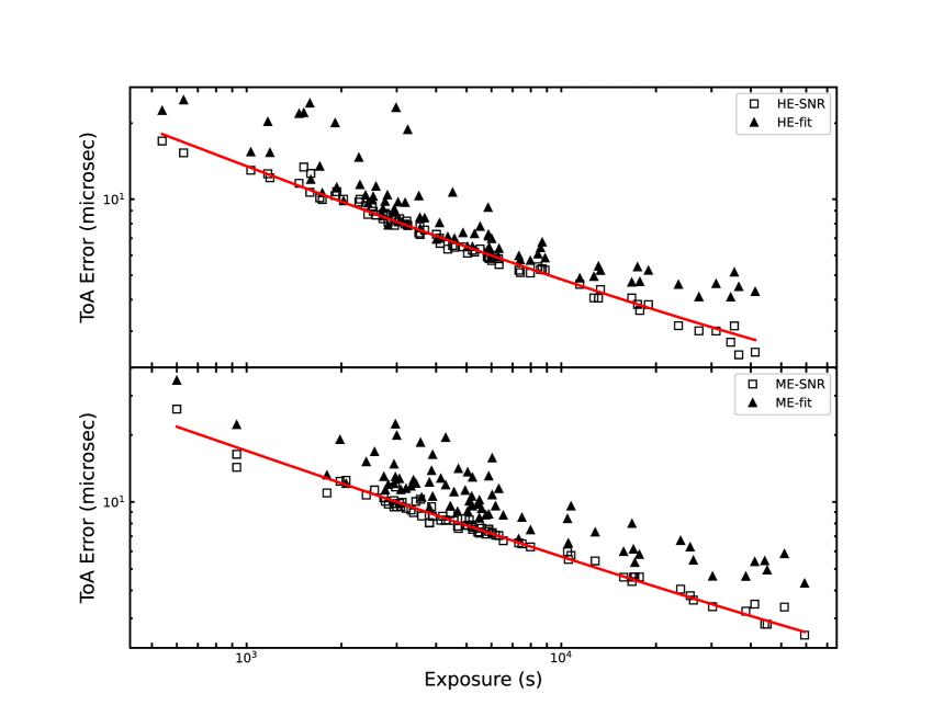
Figure 7: Top panel and the bottom panel show the relation between the ToA errors and the exposure time of corresponding profiles for HE, and ME, respectively. The errors of ToAs calculated from the signal-to-noise ratios of the main peak are presented as squares. And the errors the ToA fits are plotted as triangles. The red lines indicate the linear relation to the square root of the exposure time.

4 Timing results

4.1 Results of Jodrell Bank radio ephemeris for the Crab pulsar

The JPL-DE200 solar system ephemeris is adopted to convert the arrival time of photons to the barycenter of the solar system. After the solar barycenter corrections, the epoch-folding method (Leahy, 1987) is used to search for the frequencies and to obtain the pulse profiles and periodic signals of the Crab pulsar. The total pulse profiles for the Crab pulsar observed by Insight-HXMT in three energy bands (LE:1–10 keV, ME:10–30 keV, HE:27–250 keV) are shown in Figure 8. The counts are normalized by scaling the counts of the main peak to unity and shifting the mean value of the background phase (0.6–0.8) to zero. The Crab’s pulse profiles have high signal-to-noise ratio due to the pointing observation mode and the large effective areas of the payloads on-board Insight-HXMT. The main pulse of LE is delayed by $864.7\text{\,}\mathrm{\SIUnitSymbolMicro s}$ compared to NICER/XTI. The accurate offset of LE is measured by the method in section 4.2. The detailed processes of instrumental delay are described in Appendix A.

The periods of the Crab pulsar measured on these 78 observations are plotted in Figure 9. The well-known spin-down trend of the Crab pulsar can be revealed and the period agrees with the radio measurements (Lyne et al., 1993) at the Jodrell Bank observatory within 0.1 ns.

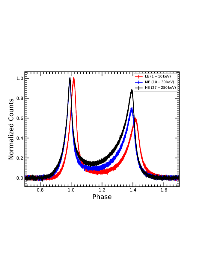
Figure 8: The pulse profile of the Crab pulsar observed by Insight-HXMT in three energy bands, using the Jodrell Bank Crab ephemeris. The red, blue, and black lines indicate the profiles of the three payloads of Insight-HXMT, LE (1–10 keV), ME (10–30 keV), and HE (27–250 keV), respectively. For clarify the phase is plotted from 0.7 to 1.7. The counts are normalized by scaling the counts of the main peak to unity and shifting the mean value of the background phase (0.6–0.8) to zero. The LE profile is significantly delayed by LE’s readout mechanism (see text for details).

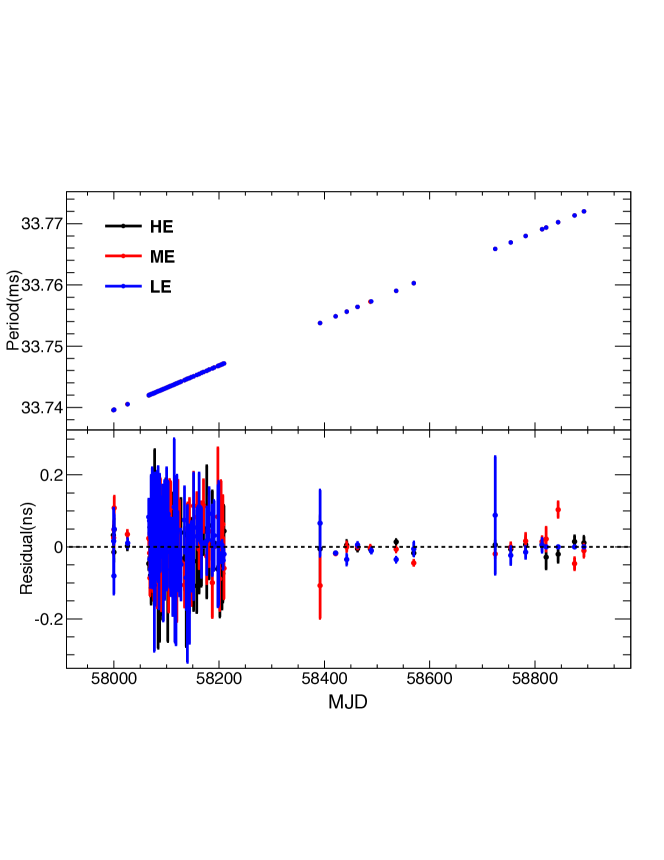
Figure 9: The top panel shows the periods of the Crab pulsar obtained by Insight-HXMT on different dates. The bottom panel shows the difference between our results and those from radio measurements at the Jodrell Bank observatory.

4.2 Offset and systematic errors of Insight-HXMT timing system

The offset and the systematic errors of Insight-HXMT’s timing system can be revealed by measuring the evolution of the absolute phase of the main peak over time. At first we investigate the systematic error using the Jodrell Bank radio ephemeris, similar to INTEGRAL/SPI (Kuiper et al., 2003; Molkov et al., 2010), and RXTE/PCA (Rots et al., 2004). The systematic error of Insight-HXMT timing system is within $45\text{\,}\mathrm{\SIUnitSymbolMicro s}$. Similar results have been reported in RXTE observations, where the systematic error due to the interstellar scattering and instrumental calibration of radio telescope is dominant (Rots et al., 2004; Ge et al., 2012). Because this systematic error is relatively high, it is not precise enough to calibrate the timing system of Insight-HXMT by directly using the radio ephemeris. Therefore, we use the quasi-simultaneous observations on the Crab with NICER to produce the Crab ephemeris and then estimate the offset and systematic errors of Insight-HXMT, given the good timing performance of NICER/XTI (Enoto et al., 2021).

The procedures for generating Crab pulsar’s ephemeris using NICER/XTI observations are described in the following. We redo the barycentric correction using JPL-DE405 solar system ephemeris for the data of quasi-simultaneous NICER and Insight-HXMT Crab observations. The spinning frequency and the pulse profile from each NICER observation are obtained by the frequency search procedure mentioned in section 3.2. ToAs and their errors are calculated based on the pulse profiles using the fitting method mentioned in section 3.3. The timing parameters are obtained by fitting the evolution of ToAs over time using TEMPO2 (Hobbs et al., 2006). This set of timing parameters is then used to epoch-fold the pulse profile and calculate a new set of ToAs. By iterate the above procedure of fitting and calculating ToAs, the timing parameters and ToAs converge to stable values. The ephemeris containing the timing parameters obtained by NICER/XTI data is listed in Table 3.

Parameter	Time range 1	Time range 2
RA (J2000)	$05^{\rm{h}}34^{\rm{m}}31^{\rm{s}}.973$
DEC (J2000)	$22^{\circ}00^{\prime}52^{\prime\prime}.069$
START (MJD)	58064.99	58070.99
STOP (MJD)	58071.01	58078.01
$t_{0}$ (MJD;TDB)	58068	58080
$f_{0}$ (Hz)	29.63662156(2)	29.63623713(1)
$f_{1}$ ($10^{-10}\,\rm{Hz}\,\rm{s}^{-1}$)	-3.701(4)	-3.704(1)
$f_{2}$ ($10^{-18}\,\rm{Hz}\,\rm{s}^{-2}$)	-7(4).252	2(1).382
$f_{3}$ ($10^{-23}\,\rm{Hz}\,\rm{s}^{-3}$)	5(4).431	0.5(2)02

Table 3: Crab ephemeris fitted by NICER observations which are simultaneously with Insight-HXMT.

Since the timing parameters of the Crab pulsar have been obtained from NICER observations, the positions of the main peak observed by Insight-HXMT can be measured from the epoch-folded pulse profiles. As shown in Figure 10, the main peak position of each observation are plotted in different colors for LE (in purple), ME (in red), HE (in black), and NICER/XTI (in blue). The dashed lines are the weighted mean positions of each payload respectively.

We define the offset as the deviation of the observed main peak position that observed by NICER. The offsets of Insight-HXMT are displayed in Table 4. The systematic errors and mean phase can be derived using the same method from equation (11) in Li et al. (2020) and the results are also displayed in Table 4.

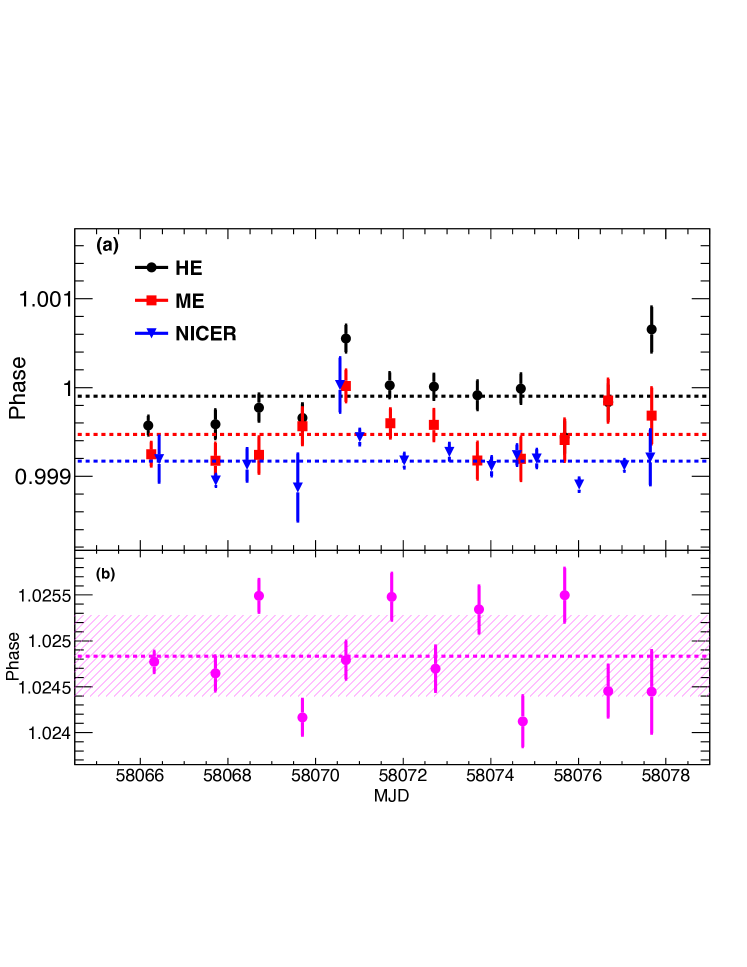
Figure 10: The top panel shows the best-fit values of the main pulse positions of the Crab pulsar using the timing ephemerides of NICER. The black points, red squares, and blue triangles are the results for HE, ME, and NICER respectively. The corresponding dotted lines are the mean phases for them. The bottom panel shows the best-fit values of the main pulse positions of Crab pulsar for LE. The purple dotted line is the mean phase for LE. The purple slashed area show the 1$\sigma$ (systematic error) confidence intervals for the mean phase.

Table 4: The timing errors of Insight-HXMT payloads respect to NICER.

Payloads	mean	systematic	statistic	offset
	phase	error ($\mathrm{\SIUnitSymbolMicro s}$)	error ($\mathrm{\SIUnitSymbolMicro s}$)	($\mathrm{\SIUnitSymbolMicro s}$)
NICER	0.999172	5.5	0.9	0
HE	0.999904	12.1	1.5	24.7
ME	0.999472	8.6	1.9	10.1
LE	1.02483	15.8	2.1	864.7

4.3 Delay evolution with energy

The deviation of the main peak obtained by ME and HE respect to NICER/XTI observation is caused mainly by the intrinsic property of the Crab pulsar, because the instrumental time delay is about $0.334\text{\,}\mathrm{\SIUnitSymbolMicro s}$ and $0.156\text{\,}\mathrm{\SIUnitSymbolMicro s}$ for ME and HE, respectively. The instrumental delays estimated by the electronic design are described in Appendix A.

The broad band observations on the pulsar indicate that the main peak phase of the Crab pulsar changes with energy (Molkov et al., 2010). The energy resolved phase of HXMT delay to the NICER main peak can be determined as previously described. We split XTI, ME, and HE data in the first duration mentioned in Table 3 into three energy bands, and get the position of the main peak in each energy band by Gaussian fitting. Figure 11 shows the evolution of the peak position versus energy with respect to the 1–3 keV peak position obtained from NICER/XTI. We select the main peak position of NICER XTI data in 1–3 keV as reference position and calculate the delay of the main peak of difference profiles with different energy, as shown in Figure 11. In order to compare with the results reported in Molkov et al. (2010), a $304\text{\,}\mathrm{\SIUnitSymbolMicro s}$ radio delay compared to NICER/XTI (Enoto et al., 2021) is added to the offsets measured. Since the relative offsets of Insight-HXMT compared with NICER/XTI for 1–3 keV have already been known, the radio delay relative to HXMT can also be derived as shown in Figure 11.

The delay decreases with energy at a rate of $0.26\pm 0.02$ $\mathrm{\SIUnitSymbolMicro s}\text{\,}{\mathrm{keV}}^{-1}$ by a linear fitting using the NICER and HXMT data. The radio delays of RXTE/PCA, HEXTE and INTEGRAL/SPI reported in (Molkov et al., 2010) are also shifted downward by about $10\text{\,}\mathrm{\SIUnitSymbolMicro s}$ and shown in Figure 11. The results of RXTE are generally consistent with the linear trend, but the results from INTEGRAL/SPI with large uncertainties is lower than the linear trend. This rate is smaller than the value reported in Molkov et al. (2010) $0.6\pm 0.2$ $\mathrm{\SIUnitSymbolMicro s}$, but consistent within $2\sigma$.

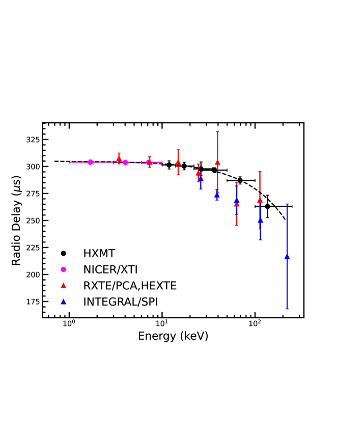
Figure 11: Radio delay of the main peak position for the Crab pulsar compared to the X-ray at different energies. The main peak delays of Insight-HXMT/HE and Insight-HXMT/ME with respect to NICER/XTI are calculated. Considering the radio delay of $304\text{\,}\mathrm{\SIUnitSymbolMicro s}$ compared to XTI reported in Enoto et al. (2021), we obtain the radio delay as a function of X-ray energy. The data are collected from NICER and Insight-HXMT, covering 1–250 keV. The black dashed line is the best-fit to the data points of HE, ME, and XTI with a linear function. The purple NICER and black Insight-HXMT results are from this work. The radio delays of RXTE/PCA, HEXTE (red triangles) and INTEGRAL/SPI (blue triangles) reported in Molkov et al. (2010) are shifted downward by about $10\text{\,}\mathrm{\SIUnitSymbolMicro s}$ for comparison.

5 Conclusions

We have investigated the stability and accuracy of the timing system of Insight-HXMT with the observation of the Crab pulsar. We find that the systematic errors of HE, ME, and LE are $12.1\text{\,}\mathrm{\SIUnitSymbolMicro s}$, $8.6\text{\,}\mathrm{\SIUnitSymbolMicro s}$, and $15.8\text{\,}\mathrm{\SIUnitSymbolMicro s}$, respectively. The offsets obtained from the ToAs of Crab pulsar with respect to the NICER measurements are HE: $24.7\text{\,}\mathrm{\SIUnitSymbolMicro s}$, and ME: $10.1\text{\,}\mathrm{\SIUnitSymbolMicro s}$. The non-physical offset of LE to NICER is  $864.7\text{\,}\mathrm{\SIUnitSymbolMicro s}$ due to the special readout mechanism.

Jointly using the NICER and Insight-HXMT data, the evolution of Crab pulsar’s main peak position can be well fitted by a linear function of $0.26\pm 0.02$ $\mathrm{\SIUnitSymbolMicro s}\text{\,}{\mathrm{keV}}^{-1}$, which is smaller than but consistent with the results of Molkov et al. (2010) within $2\sigma$ confidence range.

Appendix A Internal instrumental delay

It is essential to provide the instrumental delay of the photons for studying the energy-dependence of the Crab main pulse and comparing the results with other instruments. The time system is corrected by the PPS signal, so the offset of the X-ray photons recording time related to PPS signal represents the instrumental delay. The total instrumental delay can be estimated by accumulating the typical response time of each electronic device in the electronic design.

For Insight-HXMT/HE and Insight-HXMT/ME, the electronic design are shown in Figure 12 and Figure 13. The delays are $0.156\text{\,}\mathrm{\SIUnitSymbolMicro s}$ and $0.335\text{\,}\mathrm{\SIUnitSymbolMicro s}$, respectively. The instrumental delays for HE and ME are negligible, compared to the energy-dependent evolution of $0.26\text{\,}\mathrm{\SIUnitSymbolMicro s}\text{\,}{\mathrm{keV}}^{-1}$ as discussed in 4.1.

The electronic design of Insight-HXMT/LE is shown in Figure 14, in which the total delay is $864\text{\,}\mathrm{\SIUnitSymbolMicro s}$. The delay of LE is mainly due to the special readout mechanism of the swept charge devices for LE (Zhao et al., 2019; Zhou et al., 2021). We note that Zhao et al. (2019) reported the probability distribution of the delay time, in which the distributions are measured both in-orbit and on-ground. The delay probability distribution is very different between the pre-launch and the in-orbit measurements, because there were no collimators installed during the on-ground measurement. To get the delay of this readout mechanism of LE, the pulse profile of the Crab pulsar measured by NICER is convolved with the delay distribution measured in-orbit. The peak of the main pulse is delayed by $856\text{\,}\mathrm{\SIUnitSymbolMicro s}$ to the real pulse profile. The electronic process also takes about $8\text{\,}\mathrm{\SIUnitSymbolMicro s}$ delay before it sends the signal to the FPGA of LE box as shown in Figure 14. Therefore, the total delay of LE is about $864\text{\,}\mathrm{\SIUnitSymbolMicro s}$, which is similar to the measured phase shift of the Crab pulsar compared with NICER.

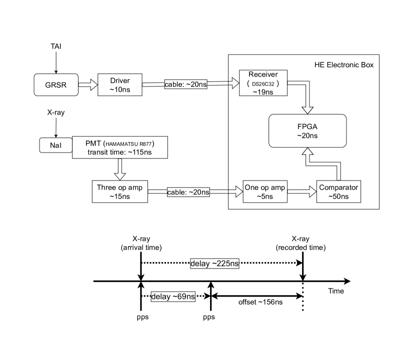
Figure 12: The upper diagram is the electronic design of the Insight-HXMT/HE, and the lower diagram indicates the internal instrumental delay of detected X-ray photons. The PPS signal and X-ray photons are recorded by the FPGA through different electronic processes. For the PPS signal, the GPS receiver (GPSR) receives the international atomic time (TAI) signal and then passes through a driver that produces a $10\text{\,}\mathrm{ns}$ delay. The PPS then travels at a speed of $5\text{\,}\mathrm{ns}\text{\,}{\mathrm{m}}^{-1}$ over a cable of about $4\text{\,}\mathrm{m}$ to the HE electronic box. One receiver spends $19\text{\,}\mathrm{ns}$ in signal processing. The FPGA sampling process generates another $20\text{\,}\mathrm{ns}$ delay. For X-ray photons, after depositing in NaI crystal, the photo-electrons are generated by the PMT and the transit time of PMT produces a delay of $115\text{\,}\mathrm{ns}$. After three operational amplifiers (generating a delay of $15\text{\,}\mathrm{ns}$), and through about $4\text{\,}\mathrm{m}$ of cable (about $20\text{\,}\mathrm{ns}$ delay), it reaches the HE electronic box. Through another operational amplifier (about $5\text{\,}\mathrm{ns}$) and a comparator (generating a delay of $50\text{\,}\mathrm{ns}$), it arrives at the FPGA and is recorded. A $20\text{\,}\mathrm{ns}$ of sampling time is also required for the FPGA to process the X-ray photons. The lower diagram indicate that the X-ray photons have approximately $156\text{\,}\mathrm{ns}$ offset to the GPS PPS signal.

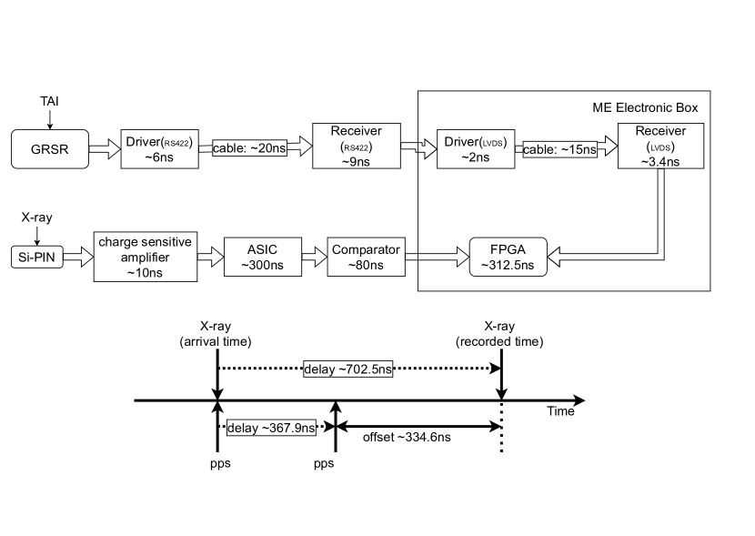
Figure 13: The upper diagram is the electronic design of the Insight-HXMT/ME, and the lower diagram indicates the internal instrumental delay of detected X-ray photons. For the PPS signal, the GPS receiver (GPSR) receives the international atomic time (TAI) signal and then passes through a driver that produces a $6\text{\,}\mathrm{ns}$ delay. The PPS then travels at a speed of $5\text{\,}\mathrm{ns}\text{\,}{\mathrm{m}}^{-1}$ over a cable of about $4\text{\,}\mathrm{m}$. Then it is processed by a receiver, which generates a $9\text{\,}\mathrm{ns}$ delay. In the ME electronic box, a signal passes through another driver (costs $2\text{\,}\mathrm{ns}$), a $3\text{\,}\mathrm{m}$ cable (costs $15\text{\,}\mathrm{ns}$), and another receiver (costs $3.4\text{\,}\mathrm{ns}$) and is recorded by the FPGA. The FPGA sampling process generates a $312.5\text{\,}\mathrm{ns}$ delay. The total delay of PPS signal is about $367.9\text{\,}\mathrm{ns}$, as indicated in the lower diagram. For X-ray photons, they are detected by Si-PIN detector. The charge sensitive amplifier processes the signal and produces a $10\text{\,}\mathrm{ns}$ delay. Through the ASIC ($300\text{\,}\mathrm{ns}$) and a comparator ($80\text{\,}\mathrm{ns}$ delay), it recorded by the FPGA in the ME electronic box. The total delay of an X-ray photon is about $702.5\text{\,}\mathrm{ns}$, as indicated in the lower diagram. The offset of X-ray photons compared to PPS is about $334.6\text{\,}\mathrm{ns}$.

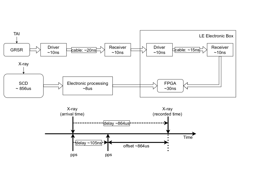
Figure 14: The upper diagram is the electronic design of the Insight-HXMT/LE, and the lower diagram indicates the internal instrumental delay of detected X-ray photons. For the PPS signal, the electronic processes are similar to ME design. The GPS receiver (GPSR) receives the international atomic time (TAI) signal and then passes through a driver that produces a $10\text{\,}\mathrm{ns}$ delay. The PPS then travels at a speed of $5\text{\,}\mathrm{ns}\text{\,}{\mathrm{m}}^{-1}$ over a cable of about $4\text{\,}\mathrm{m}$. Then it is processed by a receiver, which generates a $10\text{\,}\mathrm{ns}$ delay. In the LE electronic box, a signal passes through another driver, a $3\text{\,}\mathrm{m}$ cable, and another receiver and is recorded by the FPGA. The FPGA sampling process generates a $30\text{\,}\mathrm{ns}$ delay. The total delay of PPS signal is about $105\text{\,}\mathrm{ns}$, as indicated in the lower diagram. For X-ray photons detected by LE SCD detectors, the delay is mainly contributed by the special read-out mechanism. The main pulse of the Crab pulsar will b delayed by $856\text{\,}\mathrm{\SIUnitSymbolMicro s}$. The total electronic processes produce about $8\text{\,}\mathrm{\SIUnitSymbolMicro s}$ delay. Thus the instrumental offset of X-ray photons of LE is about $864\text{\,}\mathrm{\SIUnitSymbolMicro s}$, as indicated in the lower diagram.

References

- Aliu et al. (2011) Aliu, E., Arlen, T., Aune, T., et al. 2011, Science, 334, 69
- Cao et al. (2020) Cao, X., Jiang, W., Meng, B., et al. 2020, SCIENCE CHINA Physics, Mechanics & Astronomy, 63, 1
- Chen et al. (2020) Chen, Y., Cui, W., Li, W., et al. 2020, SCIENCE CHINA Physics, Mechanics & Astronomy, 63, 1
- Enoto et al. (2021) Enoto, T., Terasawa, T., Kisaka, S., et al. 2021, Science, 372, 187
- Ge et al. (2012) Ge, M., Lu, F., Qu, J. L., et al. 2012, The Astrophysical Journal Supplement Series, 199, 32
- Guillot et al. (2019) Guillot, S., Kerr, M., Ray, P. S., et al. 2019, The Astrophysical Journal Letters, 887, L27
- Guo et al. (2020) Guo, C.-C., Liao, J.-Y., Zhang, S., et al. 2020, Journal of High Energy Astrophysics, 27, 44, doi: 10.1016/j.jheap.2020.02.008
- Hobbs et al. (2006) Hobbs, G. B., Edwards, R. T., & Manchester, R. N. 2006, MNRAS, 369, 655, doi: 10.1111/j.1365-2966.2006.10302.x
- Kuiper et al. (2003) Kuiper, L., Hermsen, W., Walter, R., & Foschini, L. 2003, Astronomy & Astrophysics, 411, L31
- Leahy (1987) Leahy, D. 1987, Astronomy and Astrophysics, 180, 275
- Li et al. (2020) Li, X., Li, X., Tan, Y., et al. 2020, Journal of High Energy Astrophysics, 27, 64
- Liao et al. (2020a) Liao, J.-Y., Zhang, S., Lu, X.-F., et al. 2020a, Journal of High Energy Astrophysics, 27, 14, doi: 10.1016/j.jheap.2020.04.002
- Liao et al. (2020b) Liao, J.-Y., Zhang, S., Chen, Y., et al. 2020b, Journal of High Energy Astrophysics, 27, 24, doi: 10.1016/j.jheap.2020.02.010
- Liu et al. (2020) Liu, C., Zhang, Y., Li, X., et al. 2020, Science China Physics, Mechanics, and Astronomy, 63, 249503, doi: 10.1007/s11433-019-1486-x
- Lorimer & Kramer (2012) Lorimer, D. R., & Kramer, M. 2012, Handbook of Pulsar Astronomy
- Lu & Zhang (2018) Lu, F., & Zhang, S. 2018, Chin. J. Space Sci, 38, 72
- Lyne et al. (1993) Lyne, A., Pritchard, R., & Graham Smith, F. 1993, Monthly Notices of the Royal Astronomical Society, 265, 1003
- Molkov et al. (2010) Molkov, S., Jourdain, E., & Roques, J. P. 2010, ApJ, 708, 403, doi: 10.1088/0004-637X/708/1/403
- Rots et al. (2004) Rots, A. H., Jahoda, K., & Lyne, A. G. 2004, The Astrophysical Journal Letters, 605, L129
- Terada et al. (2008) Terada, Y., Enoto, T., Miyawaki, R., et al. 2008, Publications of the Astronomical Society of Japan, 60, S25
- Zhang et al. (2020) Zhang, S.-N., Li, T., Lu, F., et al. 2020, SCIENCE CHINA Physics, Mechanics & Astronomy, 63, 1
- Zhao et al. (2019) Zhao, X.-F., Zhu, Y.-X., Han, D.-W., et al. 2019, Journal of High Energy Astrophysics, 23, 23
- Zheng et al. (2019) Zheng, S. J., Zhang, S. N., Lu, F. J., et al. 2019, ApJS, 244, 1, doi: 10.3847/1538-4365/ab3718
- Zhou et al. (2021) Zhou, D.-K., Zheng, S.-J., Song, L.-M., et al. 2021, Research in Astronomy and Astrophysics, 21, 005