Limits of Lateral Expansion in Two-Dimensional Materials with Line Defects

Abstract

The flexibility of two-dimensional (2D) materials enables static and dynamic ripples that are known to cause lateral contraction, shrinking of the material boundary. However, the limits of 2D materials’ lateral expansion are unknown. Therefore, here we discuss the limits of intrinsic lateral expansion of 2D materials that are modified by compressive line defects. Using thin sheet elasticity theory and sequential multiscale modeling, we find that the lateral expansion is inevitably limited by the onset of rippling. The maximum lateral expansion $\chi_{\text{max}}\approx 2.1\cdot t^{2}\sigma_{d}$, governed by the elastic thickness $t$ and the defect density $\sigma_{d}$, remains typically well below one percent. In addition to providing insight to the limits of 2D materials’ mechanical limits and applications, the results highlight the potential of line defects in strain engineering, since for graphene they suggest giant pseudomagnetic fields that can exceed $1000$ T.

The discoveries of two-dimensional (2D) materials were followed by reports of their subtle mechanical properties  [1]. They are never fully flat, since their elastic thinness make them susceptible for stabilizing out-of-plane rippling  [2, 3, 4]. Rippling also implies in-plane softening and considerable out-of-plane stiffening  [5, 6, 7]. However, materials’ high in-plane stiffness keeps their surface area unchanged, which implies lateral contraction, shrinking of the material boundary [8]. This effect is best known from the negative thermal expansion coefficient of graphene [9, 10, 11].

Rippling and lateral contraction are relevant for several reasons. Ripples affect substrate adhesion (and vice versa) as well as in-plane and out-of-plane deformations [12, 13, 14, 15, 16, 17]. They can be created by point defects [18], adsorbates [19], grain boundaries [20, 21], or line defects [6], also without excessive hampering of material’s mechanical and electronic properties [22]. Contraction influences the functioning of nanoscale devices such as resonators and facilitates strain engineering to control both mechanical and electronic properties [23, 4]. However, despite the prominence of rippling and contraction in practical applications and the abundance of related literature, one fundamental question remains open: what are the limits of intrinsic lateral expansion for 2D materials?

An attractive strategy to address this question is to consider 2D materials with compressive line defects. The line defects can act as tiny stitches that can induce local stretched areas that—so the argument goes—cumulate into global lateral expansion [6]. Representing various physical origins such as dislocations [24], adsorbate arrays [19, 25, 26], stacking variations [27], heterostructure interfaces [28], or grain boundaries [29, 30], line defects allow creating local compressive stress at relatively low defect density. While some line defects are created during material synthesis, others can be created afterwards by chemical means or even by direct laser irradiation [31, 32].

In this Letter I use thin sheet elasticity theory and sequential multiscale modeling to investigate the lateral expansion limits of 2D materials with compressive line defects. Theory permits analytical models with simple expressions for ripple properties and lateral expansion. It turns out that lateral expansion and rippling cannot coexist; rippling destroys expansion effectively.

Table 1: Elastic parameters for selected 2D materials.

Material	$k_{s}$ (eV/Å2)	$k_{b}$ (eV)	$\nu$	$t$ (Å)
Graphene [33]	21	1.5	0.15	0.93
Bilayer graphene[34]	42	180	0.15	7.2
MoS2 [35, 36]	8	12	0.3	4.2
BN [33]	17	1.3	0.2	0.96
Silicene [37, 38]	3.8	0.4	0.4	1.1

To model the defected 2D materials, I invoke the thin sheet elasticity theory [39], because it has proven effective and reliable even for atomic-scale deformations [33, 40, 41, 42, 43, 44, 45, 46, 1]. Theory characterizes membranes by bending modulus $k_{b}$, Poisson ratio $\nu$, and 2D Young’s modulus $k_{s}$. Membrane’s intrinsic length scale is given by the elastic thickness

$$t=\sqrt{12k_{b}/M},$$ (1)

where $M=k_{s}/(1-\nu^{2})$ is the longitudinal modulus. Elastic thickness equals the physical thickness of the 2D material when viewed as a slab of isotropic elastic membrane. Table 1 shows parameters for selected 2D materials [33, 34, 35, 36, 37, 38].

The theory can be augmented to include compressive line defects, modeling them as stripes of width $a$, length $l$, and a pre-strain $\varepsilon_{0}$ that implies the equilibrium length $l(1+\varepsilon_{0})$ (Fig. 1a) [6]. The magnitude of $a$ is around $2-3$ Å as it arises from the atomic structure of the defect [6]. The parameter

$$\mathcal{S}=a\varepsilon_{0}$$ (2)

characterizes the strength of the line defect. For small deformations (strains $\ll\varepsilon_{0}$) the line defect corresponds to one-dimensional line stress $\tau=M\mathcal{S}$. The strength $\mathcal{S}$ is unique for given 2D material and line defect, but here I treat it as a continuous parameter. I ignore tensile pre-strain ($\varepsilon_{0}<0$), because it cannot induce lateral expansion in any situation. Based on earlier atomic simulations, reasonable compressive pre-strains lie in the range $\varepsilon_{0}\lesssim 20$ % [6].

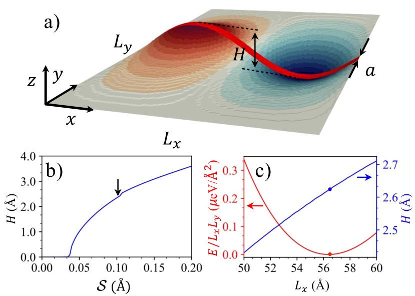
Figure 1: Rippling of $5$ nm$\times 10$ nm 2D membrane ($t=1.0$ Å) by an infinitely long compressive line defect. a) One ripple wavelength from a line defect with $\mathcal{S}=0.1$ Å ($a=2.5$ Å and $\varepsilon_{0}=4$ %). Vertical dimension is scaled by a factor of five and the width of the line defect is exaggerated. b) Ripple height $H$ as a function of the line defect strength $\mathcal{S}$. The membrane buckles at $\mathcal{S}=0.04$ Å; the arrow points the geometry in panel a. c) Surface energy density (left scale) and ripple height (right scale) as a function of ripple wavelength $\lambda=L_{x}$ for $\mathcal{S}=0.1$ Å.

The theory was then harnessed for numerical simulations of defected membranes in an $L_{x}\times L_{y}$ periodic rectangular cell. Membrane was discretized to an $N_{x}\times N_{y}$ grid and the optimum morphology was solved numerically by minimizing the total elastic energy; see Supplemental Material (SM) for details [47]. Materials of different elastic thicknesses $t=1.0\ldots 10$ Å were simulated by adopting a fixed Poisson ratio ($\nu=0.15$) and longitudinal modulus ($M=21.5$ eV/Ų) while varying $k_{b}$ according to Eq. (1). Line defect strengths $\mathcal{S}$ were adjusted by choosing the width equal to a typical lattice constant $a=2.5$ Å and varying $\varepsilon_{0}$. Since the main parameters are $t$ and $\mathcal{S}$, the above choices do not restrict the general validity of the results. In the numerical implementation, because the atomic scale is much smaller than the grid spacing ($a\ll L_{x}/N_{x}$), the line defects were introduced via a sequential multiscale model (SM) [47].

To construct a comprehensive understanding of the effect of line defects, I start by discussing isolated infinite and finite line defects before analyzing experimentally relevant random line defect networks.

Consider a $5\text{ nm}\times 10\text{ nm}$ membrane with $t=1.0$ Å and an infinitely long ($l=L_{x}$) line defect along $x$-axis (Fig. 1a). The membrane is initially planar, but buckles to a rippled conformation upon increasing line defect strength from zero to $\mathcal{S}=0.04$ Å (Figs 1 a and b). The ripple forms because it releases the compressive stress of the line defect. Further increase in $\mathcal{S}$ leads to monotonous increase in ripple height. The ripple height profile can be approximated by the sine wave

$$z(x,y)=\tfrac{1}{2}H\exp{\left(-y^{2}/2\sigma^{2}\right)}\sin{(2\pi x/\lambda)},$$ (3)

where $H$ is the peak-to-peak height, $\lambda$ is the wavelength, and $\sigma$ is a measure for the lateral width of the ripple.

The above choice of $L_{y}=10$ nm was irrelevant because the ripple decays exponentially in $y$-direction. However, the choice of $L_{x}$ must be investigated in detail, as it directly determines the ripple wavelength. Fixing $\mathcal{S}=0.1$ Å and increasing $L_{x}$ leads to monotonously increasing ripple height and a minimum of the surface energy density $E/(L_{x}L_{y})$ at $L_{x}=56.3$ Å with $H=2.62$ Å (Fig. 1c). This minimum implies that the ripple wavelength in an extended system is $\lambda=56.3$ Å.

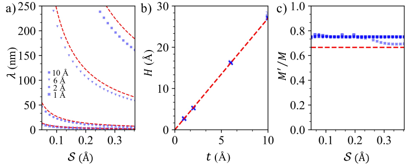
Figure 2: Ripple trends with infinite line defects. a) Optimum ripple wavelength as a function of line defect strength for different $t$. b) Ripple height as a function of elastic thickness. c) Longitudinal constant $M^{\prime}$ of the entire simulation cell as a function of line defect strength. All panels show both numerical simulations (symbols) and analytical estimates [dashed lines from Eq. (4) for $\lambda$, Eq. (5) for $H$ and Eq. (S14) for $M^{\prime}$]. $L_{x}=\lambda$ and $L_{y}=1.5\cdot\lambda$ in all panels.

The rippling with line defects can be investigated also analytically. As derived in SM, adopting the ripple profile (3) leads to the estimates for the optimum wavelength as

$$\lambda=6.8\cdot t^{2}/\mathcal{S},$$ (4)

for the ripple height as,

$$H=2.7\cdot t$$ (5)

and for the ripple width as $\sigma\approx\lambda/5$ [47]. The estimates suggest that wavelengths increase for elastically thicker membranes and weaker line defects, which is plausible when viewed in terms of energy; shorter ripples require more energy, which is available in stronger line defects. Unexpectedly, however, the ripple height $H$ depends only on elastic thickness and is independent of the properties of the line defect. This implies that ripples would form even with very weak line defects—although with very long wavelengths. In addition, the analytical model provides estimates for maximal slopes $\max(|dz/dx|)=1.2\cdot\mathcal{S}/t$, curvatures $\max(\mathcal{C}_{xx})=\mathcal{S}^{2}/t^{3}$, and strains $\max(\varepsilon_{xx})=0.4\cdot(\mathcal{S}/t)^{2}$ (SM) [47]. For graphene, the strain field implies pseudomagnetic fields equal to $5\cdot 10^{4}\cdot\mathcal{S}^{3}$ Å^-3T (SM) [47, 48, 49, 50]. For example, graphene with $\mathcal{S}=0.3$ Å suggests maximal slopes $0.36$, curvatures $0.27$ nm^-1, local strains $3$ %, and pseudomagnetic field that exceeds $1000$ T.

The analytical results are confirmed by systematic numerical simulations with $t=1...10$ Å and $\mathcal{S}=0...0.37$ Å. As Eqs. (4) and (5) predict, ripple wavelengths are inversely proportional to $\mathcal{S}$ and quadratically proportional to $t$ (Fig. 2a), while ripple amplitude is directly proportional to the elastic thickness, independent of $\mathcal{S}$ (Fig. 2b).

This $\mathcal{S}$-independence of $H$ brings about a curious effect for lateral elastic properties. The longitudinal modulus $M^{\prime}$ of the entire simulation cell, which accounts also for rippling, becomes entirely constant—independent of either $t$ or $\mathcal{S}$ (Fig. 2c). Governing the energy curvature upon straining $L_{x}$, the longitudinal modulus depends on the width of the simulation cell, which here is $L_{y}=1.5\cdot L_{x}$. The constancy of $M^{\prime}$ can be understood as follows: on one hand larger $t$ increases rippling height [Eq. (5)] and thereby tends to decrease $M^{\prime}$, but on the other hand larger $t$ increases bending stiffness and thereby tends to increase $M^{\prime}$. Combined, these two tendencies cancel and $M^{\prime}$ becomes approximately constant. An analytical calculation gives the estimate $M^{\prime}/M=\left(1-0.5\cdot\lambda/L_{y}\right)$ which becomes $0.67$ for current parameters (Fig. 2c; SM) [47].

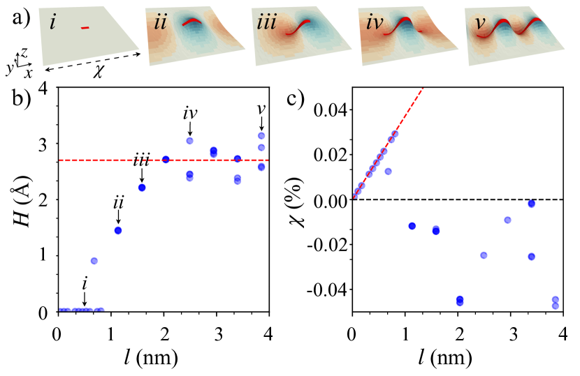
Figure 3: Lateral uniaxial expansion of $10$ nm$\times 6.6$ nm membrane with $t=1.0$ Å for line defects with $\mathcal{S}=0.25$ Å and finite length $l$. a) Development of ripple morphology with increasing $l$. The vertical dimension is scaled by a factor of five (see panel b for the color scale). b) Ripple height as a function of $l$. The arrows point at geometries in panel a. The red dashed line shows the ripple height estimate from Eq. (5) for infinitely long defects. c) Lateral expansion of the membrane in $x$-direction. The red dashed line is the estimate from Eq. (6). Fluctuations for given $l$ are due to sampling of random initial guesses.

Infinitely long line defects with optimum-wavelength ripples imply that the stress in $x$-direction vanishes. Any residual stress would lead to strain that changes the wavelength, creating a contradiction with the presumption of an optimum wavelength. This notion implies an intermediate result: infinitely long (length$\gg\lambda$) line defects cannot induce lateral expansion. But what about finite line defects?

To address this question, consider line defects whose lengths $l$ are around the optimal wavelength, $l\lesssim\lambda$. Let us fix $\mathcal{S}=0.25$ Å with $t=1.0$ Å and gradually increase the length $l$. Initially, at small $l$ the membrane remains flat, until at $l\approx 0.7$ Å it buckles to form a single bump (Fig. 3a). Simulations contain fluctuations due to random initial guesses. Analytical model similar to the one of infinite line defects gives the scaling $l_{b}=2.1\cdot t^{2}/\mathcal{S}\approx 0.8$ Å for the buckling limit, in fair agreement with numerical simulations (SM) [47]. After buckling, further lengthening leads to increased ripple height and development of alternating up-and-down bumps that gradually resemble the optimum ripple of the $l\gg\lambda$ limit (Fig. 3a).

Yet, unlike infinite line defects, finite line defects can induce lateral expansion. The expansion is defined as $\chi=(L_{x}-L_{x}^{0})/L_{x}^{0}$, which is obtained by minimizing energy with respect to cell length $L_{x}$ for given initial length $L_{x}^{0}$. As the main observation, the membrane expands steadily upon increasing $l$ until it buckles (Fig. 3c). The expansion is accurately described by the heuristic model

$$\chi=\mathcal{S}l/L_{x}L_{y}.$$ (6)

The model means that the hidden area of the line defect ($a\cdot l\varepsilon_{0}=l\mathcal{S}$) proportionally increases the surface area of the membrane ($L_{x}L_{y}$). With $l>l_{b}$ the membrane ripples and loses its capacity to sustain the compressive stress, rendering the expansion unpredictable.

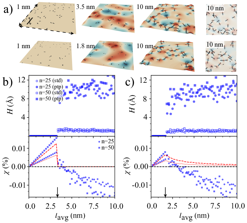
Figure 4: Lateral biaxial expansion of $100$ nm$\times 100$ nm membranes ($t=2.0$ Å) filled by networks of line defects with $\mathcal{S}=0.25$ Å. a) Ripple morphology snapshots with $50$ line defects. The networks have even (upper) and linear (lower) length distributions and increasing mean length (shown above). For clarity, the figures on the right show the networks with top views. b) Ripple peak-to-peak (ptp) and standard deviation (std) heights (upper panel) and biaxial strain (lower panel) as a function of mean defect length for $n=25$ and $n=50$ line defects with even length distribution. The red dashed line is the strain estimate from Eq. (7). c) Same as panel b for linear length distribution. Arrows point to mean lengths corresponding to the initial buckling of the longest line defects [Eq. (S22)]; for even distribution $l_{\text{max}}=l_{\text{avg}}$ and for linear distribution $l_{\text{max}}=2l_{\text{avg}}$.

These results provide sufficient insight to proceed to realistic random line defect networks [51]. I considered a $100$ nm$\times 100$ nm membrane with $n=25$ and $50$ randomly placed and oriented line defects of various lengths (Fig. 4a). The corresponding densities ($0.25\cdot 10^{12}$ cm^-2 and $0.5\cdot 10^{12}$ cm^-2) are experimentally relevant and large enough for meaningful statistics but small enough to avoid excessive interaction between the line defects [32]. The length distribution was either even ($l_{i}=l_{\text{avg}}$) or linear [$l_{i}=l_{\text{avg}}\cdot 2i/(n+1)$], where $i=1,2,\ldots n$ and $l_{\text{avg}}$ is the average length (Fig. 4a). Such distributions can be justified by previous models [51].

For a defect network with even length distribution, the membrane expands laterally upon increasing $l_{avg}$ until the buckling threshold $l_{\text{avg}}>l_{b}$ (Fig. 4b). After buckling the membrane ripples to a height that does not change much upon increasing $l_{\text{avg}}$ further. At the full $100$ nm scale the ripple height is $\sim 10$ Å  but at the local $\sim\lambda$ scale it is $\sim 5$ Å, following Eq. (5). For linear distribution the behavior is similar, only the transition to rippled membrane is less sudden. The gradual change occurs because individual line defects buckle at different $l_{\text{avg}}$. However, already the initial buckling of the longest defects ($l_{\text{max}}=2l_{avg}>l_{b}$) effectively eradicates the planar stress and destroys the lateral expansion.

The lateral expansion is described accurately for both distributions by the generalization of Eq. (6),

$$\chi=\mathcal{S}l_{\text{tot}}(l<l_{b})/L_{x}L_{y},$$ (7)

where $l_{\text{tot}}(l<l_{b})$ is the cumulative length of all line defects below the buckling length $l_{b}$ (Figs 4b and 4c). However, the membrane can sustain the lateral stress only as far as all defects remain below the buckling limit. After buckling the expansion becomes unpredictable. Ultimately, far beyond the buckling limit, the rippling strengthens and the membrane predominantly contracts [52].

Thus, 2D materials can expand laterally only when line defects remain below the buckling limit of Eq. (S22). The maximum expansion is reached when all defects have the maximum length $l_{b}$ and it equals

$$\chi_{\text{max}}\approx 2.1\cdot t^{2}\sigma_{d},$$ (8)

where $\sigma_{d}$ is the defect density. For instance, for $t=1$ Å and $\sigma_{d}=10^{12}$ cm^-2 the maximum expansion is $0.021$ %. A reasonable estimate for a optimal defect density can be obtained by assuming that one line defect occupies a minimum area of $\sim(2l_{b})^{2}$. This assumption yields the theoretical maximum for the strain as $\chi_{\text{max}}\approx\mathcal{S}^{2}/8t^{2}$. For graphene ($t=1.0$ Å) and $\mathcal{S}=0.3$ Å this implies $\chi_{\text{max}}\approx 1$ %.

Finally, I discuss briefly the role of substrates, which were excluded from the simulations. The transition from flat to rippled membranes reduces the energy by $0.13\cdot M\mathcal{S}^{3}/t^{2}$ per unit length of an infinite line defect (SM) [47]. Assuming that the defects have an effective width of $\lambda/2$, this translates into surface energy density of $0.04\cdot M(\mathcal{S}/t)^{4}$. For $M\sim 20$ eV/Ų, $t=1.0$ Å and $\mathcal{S}=0.35$ Å the energy density becomes $\sim 10$ meV/Ų—and competes with a typical strength of van der Waals adhesion [53, 54, 55]. Moreover, substrates themselves can be used for defect and strain engineering [56]. In short, a very strong adhesion can dominate membrane mechanics completely and effectively prevent both rippling and sliding. A very weak adhesion can allow for both rippling (desorption) and sliding, so that the rippling and expansion remains governed by membrane’s intrinsic dynamics. However, an intermediate adhesion can suppress rippling but still allow sliding. For such an adhesion the rippling instability would not limit the maximal intrinsic expansion anymore; the expansion would still be given by Eq. (6), but its upper limit would be given by maximum practical defect density.

To conclude, the onset of rippling dictates the limits of the lateral expansion of 2D materials. The theoretical maximum for the lateral expansion of the thinnest ($t=1$ Å) materials is around $1$ %, local strains being far greater. To diminish the effect of substrates, the expansion would be best measured experimentally from suspended 2D material samples or from customized 3D blisters of 2D materials, such as demonstrated for graphene by optical forging [7]. The simulations and analytical models presented here provide a comprehensive picture of the mechanical behavior of 2D materials with line defects and reveal new theoretical limits to open new avenues and further advance the design and strain engineering of 2D materials.

References

- Akinwande et al. [2017] D. Akinwande, C. J. Brennan, J. S. Bunch, P. Egberts, J. R. Felts, H. Gao, R. Huang, J. S. Kim, T. Li, Y. Li, K. M. Liechti, N. Lu, H. S. Park, E. J. Reed, P. Wang, B. I. Yakobson, T. Zhang, Y. W. Zhang, Y. Zhou, and Y. Zhu, A review on mechanics and mechanical properties of 2D materials, Graphene and beyond, Extreme Mechanics Letters 13, 42 (2017).
- Meyer et al. [2007] J. C. Meyer, A. K. Geim, M. I. Katsnelson, K. S. Novoselov, T. J. Booth, and S. Roth, The structure of suspended graphene sheets, Nature 446, 60 (2007).
- Lui et al. [2009] C. H. Lui, L. Liu, K. F. Mak, G. W. Flynn, and T. F. Heinz, Ultraflat graphene, Nature 462, 339 (2009).
- Deng and Berry [2016] S. Deng and V. Berry, Wrinkled, rippled and crumpled graphene: An overview of formation mechanism, electronic properties, and applications, Materials Today 19, 197 (2016).
- Blees et al. [2015] M. K. Blees, A. W. Barnard, P. a. Rose, S. P. Roberts, K. L. McGill, P. Y. Huang, A. R. Ruyack, J. W. Kevek, B. Kobrin, D. a. Muller, and P. L. McEuen, Graphene kirigami, Nature 524, 204 (2015).
- Kähärä and Koskinen [2020] T. Kähärä and P. Koskinen, Rippling of two-dimensional materials by line defects, Phys. Rev. B 075433, 075433 (2020).
- Hiltunen et al. [2021] V.-M. Hiltunen, P. Koskinen, K. K. Mentel, J. Manninen, P. Myllyperkiö, M. Pettersson, and A. Johansson, Ultrastiff graphene, 2D Materials and Applications 5, 49 (2021).
- Nicholl et al. [2017] R. J. Nicholl, N. V. Lavrik, I. Vlassiouk, B. R. Srijanto, and K. I. Bolotin, Hidden Area and Mechanical Nonlinearities in Freestanding Graphene, Physical Review Letters 118, 266101 (2017).
- Pozzo et al. [2011] M. Pozzo, D. Alfe, P. Lacovig, P. Hofmann, S. Lizzit, and A. Baraldi, Thermal expansion of supported and freestanding graphene: lattice contant versus interatomic distance, Phys. Rev. Lett. 106, 135501 (2011).
- Balandin [2011] A. A. Balandin, Thermal properties of graphene and nanostructured carbon materials, Nature Mat. 10, 569 (2011).
- Yoon et al. [2011] D. Yoon, Y.-W. Son, and H. Cheong, Negative thermal expansion coefficient of graphene measured by Raman spectroscopy, Nano Lett. 11, 3227 (2011).
- Paronyan et al. [2011] T. Paronyan, E. Pigos, and G. Chen, The Formation of Ripples in Graphene as a Result of Interfacial Instabilities, ACS nano , 9619 (2011).
- Reddy et al. [2011] C. D. Reddy, Y.-W. Zhang, and V. B. Shenoy, Influence of substrate on edge rippling in graphene sheets, Modelling and Simulation in Materials Science and Engineering 19, 054007 (2011).
- Tapasztó et al. [2012] L. Tapasztó, T. Dumitrică, S. J. Kim, P. Nemes-Incze, C. Hwang, and L. P. Biró, Breakdown of continuum mechanics for nanometre-wavelength rippling of graphene, Nature Physics 8, 739 (2012).
- Koskinen [2014] P. Koskinen, Graphene cardboard: From ripples to tunable metamaterial, Appl. Phys. Lett. 104, 101902 (2014).
- Lambin [2014] P. Lambin, Elastic Properties and Stability of Physisorbed Graphene, Applied Sciences 4, 282 (2014).
- Koskinen et al. [2018] P. Koskinen, K. Karppinen, P. Myllyperkiö, V. M. Hiltunen, A. Johansson, and M. Pettersson, Optically Forged Diffraction-Unlimited Ripples in Graphene, Journal of Physical Chemistry Letters 9, 6179 (2018).
- Zhang et al. [2014] T. Zhang, X. Li, and H. Gao, Defects controlled wrinkling and topological design in graphene, Journal of the Mechanics and Physics of Solids 67, 2 (2014).
- Thompson-Flagg et al. [2009] R. C. Thompson-Flagg, M. J. B. Moura, and M. Marder, Rippling of graphene, EPL 85, 46002 (2009).
- Malola et al. [2010] S. Malola, H. Häkkinen, and P. Koskinen, Structural, chemical, and dynamical trends in graphene grain boundaries, Phys. Rev. B 81, 165447 (2010).
- Lu et al. [2013] J. Lu, Y. Bao, C. L. Su, and K. P. Loh, Properties of strained structures and topological defects in graphene, ACS Nano 7, 8350 (2013).
- Zandiatashbar et al. [2014] A. Zandiatashbar, G. H. Lee, S. J. An, S. Lee, N. Mathew, M. Terrones, T. Hayashi, C. R. Picu, J. Hone, and N. Koratkar, Effect of defects on the intrinsic strength and stiffness of graphene, Nature Communications 5, 3186 (2014).
- Koskinen et al. [2014] P. Koskinen, I. Fampiou, and A. Ramasubramaniam, Density-Functional Tight-Binding Simulations of Curvature-Controlled Layer Decoupling and Band-Gap Tuning in Bilayer MoS2, Physical Review Letters 112, 186802 (2014).
- Warner et al. [2013] J. H. Warner, Y. Fan, A. W. Robertson, K. He, E. Yoon, and G. D. Lee, Rippling Graphene at the Nanoscale through Dislocation Addition., Nano letters 13, 4937 (2013).
- Brito et al. [2011] W. H. Brito, R. Kagimura, and R. H. Miwa, Hydrogenated grain boundaries in graphene, Applied Physics Letters 98, 213107 (2011).
- Wang et al. [2017] J. Wang, H. Yu, X. Zhou, X. Liu, R. Zhang, Z. Lu, J. Zheng, L. Gu, K. Liu, D. Wang, and L. Jiao, Probing the crystallographic orientation of two-dimensional atomic crystals with supramolecular self-assembly, Nature Communications 8, 1 (2017).
- Duerloo et al. [2014] K. A. N. Duerloo, Y. Li, and E. J. Reed, Structural phase transitions in two-dimensional Mo-and W-dichalcogenide monolayers, Nature Communications 5, 4214 (2014).
- Wang et al. [2019] J. Wang, Z. Li, H. Chen, G. Deng, and X. Niu, Nano-Micro Letters, Vol. 11 (Springer Singapore, 2019) p. 48.
- Ryder et al. [2016] C. R. Ryder, J. D. Wood, S. A. Wells, and M. C. Hersam, Chemically Tailoring Semiconducting Two-Dimensional Transition Metal Dichalcogenides and Black Phosphorus, ACS Nano 10, 3900 (2016).
- Liu and Yakobson [2010] Y. Liu and B. I. Yakobson, Cones, pringles, and grain boundary landscapes in graphene topology., Nano letters 10, 2178 (2010).
- Koivistoinen et al. [2016] J. Koivistoinen, L. Sladkova, J. Aumanen, P. J. Koskinen, K. Roberts, A. Johansson, P. Myllyperkiö, and M. Pettersson, From Seeds to Islands: Growth of Oxidized Graphene by Two-Photon Oxidation, J. Phys. Chem. C 120, 22330 (2016).
- Johansson et al. [2017] A. Johansson, P. Myllyperkiö, P. Koskinen, J. Aumanen, J. Koivistoinen, H. C. Tsai, C. H. Chen, L. Y. Chang, V. M. Hiltunen, J. J. Manninen, W. Y. Woon, and M. Pettersson, Optical Forging of Graphene into Three-Dimensional Shapes, Nano Lett. 17, 6469 (2017).
- Kudin et al. [2001] K. N. Kudin, G. E. Scuseria, and B. I. Yakobson, C2F, BN, and C nanoshell elasticity from ab initio computations, Phys. Rev. B 64, 235406 (2001).
- Koskinen and Kit [2010] P. Koskinen and O. O. Kit, Approximate Modeling of Spherical Membranes, Phys. Rev. B 82, 235420 (2010).
- Cooper et al. [2013] R. C. Cooper, C. Lee, C. A. Marianetti, X. Wei, J. Hone, and J. W. Kysar, Nonlinear elastic behavior of two-dimensional molybdenum disulfide, Physical Review B - Condensed Matter and Materials Physics 87, 035423 (2013).
- Lorenz et al. [2012] T. Lorenz, D. Teich, J. O. Joswig, and G. Seifert, Theoretical study of the mechanical behavior of individual TiS 2 and MoS 2 nanotubes, Journal of Physical Chemistry C 116, 11714 (2012).
- Peng et al. [2013] Q. Peng, X. Wen, and S. De, Mechanical stabilities of silicene, RSC Adv. 3, 13772 (2013).
- Zhao [2012] H. Zhao, Strain and chirality effects on the mechanical and electronic properties of silicene and silicane under uniaxial tension, Physics Letters, Section A: General, Atomic and Solid State Physics 376, 3546 (2012).
- Landau and Lifshitz [1986] L. D. Landau and E. M. Lifshitz, Theory of elasticity, 3rd ed. (Pergamon, New York, 1986).
- Bao et al. [2009] W. Bao, F. Miao, Z. Chen, H. Zhang, W. Jang, C. Dames, and C. N. Lau, Controlled ripple texturing of suspended graphene and ultrathin graphite membranes, Nat. Nanotechnol. 4, 562 (2009).
- Shenoy et al. [2010] V. B. Shenoy, C. D. Reddy, and Y.-W. Zhang, Spontaneous curling of graphene sheets with reconstructed edges, ACS Nano 4, 4840 (2010).
- Koskinen [2010] P. Koskinen, Electronic and optical properties of carbon nanotubes under pure bending, Phys. Rev. B 82, 193409 (2010).
- Kit et al. [2012] O. O. Kit, T. Tallinen, L. Mahadevan, J. Timonen, and P. Koskinen, Twisting Graphene Nanoribbons into Carbon Nanotubes, Phys. Rev. B 85, 085428 (2012).
- Korhonen and Koskinen [2014] T. Korhonen and P. Koskinen, Electromechanics of graphene spirals, AIP Advances 4, 127125 (2014).
- Memarian et al. [2015] F. Memarian, A. Fereidoon, and M. Darvish Ganji, Graphene Young’s modulus: Molecular mechanics and DFT treatments, Superlattices and Microstructures 85, 348 (2015).
- Koskinen [2016] P. Koskinen, Quantum Simulations of One-Dimensional Nanostructures under Arbitrary Deformations, Physical Review Applied 6, 034014 (2016).
- [47] See supplemental material at [url will be inserted by publisher] for additional results and details in analytical modeling and numerical simulations.
- Castro Neto et al. [2009] A. H. Castro Neto, F. Guinea, N. M. R. Peres, K. S. Novoselov, and A. K. Geim, The electronic properties of graphene, Rev. Mod. Phys. 81, 109 (2009).
- Kim and Castro Neto [2008] E.-A. Kim and A. H. Castro Neto, Graphene as an electronic membrane, EPL 84, 57007 (2008).
- Hsu et al. [2020] C. C. Hsu, M. L. Teague, J. Q. Wang, and N. C. Yeh, Nanoscale Strain Engineering of Giant Pseudo-Magnetic Fields, Valley Polarization and Topological Channels in Graphene, Sci. Adv. 6, eaat9488 (2020).
- Hiltunen et al. [2020] V.-M. Hiltunen, P. J. Koskinen, K. K. Mentel, J. Manninen, P. Myllyperkiö, A. Johansson, and M. Pettersson, Making Graphene Luminescent by Direct Laser Writing, The Journal of Physical Chemistry C 124, 8371 (2020).
- Liu et al. [2011] N. Liu, Z. Pan, L. Fu, C. Zhang, and B. Dai, The origin of wrinkles on transferred graphene, Nano Research 4, 996 (2011).
- Koenig et al. [2011] S. P. Koenig, N. G. Boddeti, M. L. Dunn, and J. S. Bunch, Ultrastrong adhesion of graphene membranes., Nat. Nanotechnol. 6, 543 (2011).
- Wang et al. [2016] J. Wang, D. C. Sorescu, S. Jeon, A. Belianinov, S. V. Kalinin, A. P. Baddorf, and P. Maksymovych, Atomic intercalation to measure adhesion of graphene on graphite, Nature Communications 7, 13263 (2016).
- Duong et al. [2017] D. L. Duong, S. J. Yun, and Y. H. Lee, van der Waals Layered Materials: Opportunities and Challenges, ACS Nano 11, 11803 (2017).
- Nigge et al. [2019] P. Nigge, A. C. Qu, E. Lantagne-Hurtubise, E. Marsell, S. Link, G. Tom, M. Zonno, M. Michiardi, M. Schneider, S. Zhdanovich, G. Levy, U. Starke, C. Gutierrez, D. Bonn, S. A. Burke, M. Franz, and A. Damascelli, Room temperature strain-induced Landau levels in graphene on a wafer-scale platform, Science Advances 5, eaaw5593 (2019), 1902.00514 .
- Harris et al. [2020] C. R. Harris, K. J. Millman, S. J. van der Walt, R. Gommers, P. Virtanen, D. Cournapeau, E. Wieser, J. Taylor, S. Berg, N. J. Smith, R. Kern, M. Picus, S. Hoyer, M. H. van Kerkwijk, M. Brett, A. Haldane, J. F. del Río, M. Wiebe, P. Peterson, P. Gérard-Marchant, K. Sheppard, T. Reddy, W. Weckesser, H. Abbasi, C. Gohlke, and T. E. Oliphant, Array programming with NumPy, Nature 585, 357 (2020).
- Virtanen et al. [2020] P. Virtanen, R. Gommers, T. E. Oliphant, M. Haberland, T. Reddy, D. Cournapeau, E. Burovski, P. Peterson, W. Weckesser, J. Bright, S. J. van der Walt, M. Brett, J. Wilson, K. J. Millman, N. Mayorov, A. R. Nelson, E. Jones, R. Kern, E. Larson, C. J. Carey, f. Polat, Y. Feng, E. W. Moore, J. VanderPlas, D. Laxalde, J. Perktold, R. Cimrman, I. Henriksen, E. A. Quintero, C. R. Harris, A. M. Archibald, A. H. Ribeiro, F. Pedregosa, P. van Mulbregt, A. Vijaykumar, A. P. Bardelli, A. Rothberg, A. Hilboll, A. Kloeckner, A. Scopatz, A. Lee, A. Rokem, C. N. Woods, C. Fulton, C. Masson, C. Häggström, C. Fitzgerald, D. A. Nicholson, D. R. Hagen, D. V. Pasechnik, E. Olivetti, E. Martin, E. Wieser, F. Silva, F. Lenders, F. Wilhelm, G. Young, G. A. Price, G. L. Ingold, G. E. Allen, G. R. Lee, H. Audren, I. Probst, J. P. Dietrich, J. Silterra, J. T. Webber, J. Slavič, J. Nothman, J. Buchner, J. Kulick, J. L. Schönberger, J. V. de Miranda Cardoso, J. Reimer, J. Harrington, J. L. C. Rodríguez, J. Nunez-Iglesias, J. Kuczynski, K. Tritz, M. Thoma, M. Newville, M. Kümmerer, M. Bolingbroke, M. Tartre, M. Pak, N. J. Smith, N. Nowaczyk, N. Shebanov, O. Pavlyk, P. A. Brodtkorb, P. Lee, R. T. McGibbon, R. Feldbauer, S. Lewis, S. Tygier, S. Sievert, S. Vigna, S. Peterson, S. More, T. Pudlik, T. Oshima, T. J. Pingel, T. P. Robitaille, T. Spura, T. R. Jones, T. Cera, T. Leslie, T. Zito, T. Krauss, U. Upadhyay, Y. O. Halchenko, and Y. Vázquez-Baeza, SciPy 1.0: fundamental algorithms for scientific computing in Python, Nature Methods 17, 261 (2020).
- Bitzek et al. [2006] E. Bitzek, P. Koskinen, F. Gähler, M. Moseler, and P. Gumbsch, Structural Relaxation Made Simple, Phys. Rev. Lett. 97, 170201 (2006).