The peculiar chemical pattern of the WASP-160 binary system: signatures of planetary formation and evolution?

Abstract

Wide binary stars with similar components hosting planets provide a favorable opportunity for exploring the star-planet chemical connection. We perform a detailed characterization of the solar-type stars in the WASP-160 binary system. No planet has been reported yet around WASP-160A while WASP-160B is known to host a transiting Saturn-mass planet, WASP-160B b. For this planet, we also derive updated properties from both literature and new observations. Furthermore, using TESS photometry, we constrain the presence of transiting planets around WASP-160A and additional ones around WASP-160B. The stellar characterization includes, for the first time, the computation of high-precision differential atmospheric and chemical abundances of 25 elements based on high-quality Gemini-GRACES spectra. Our analysis reveals evidence of a correlation between the differential abundances and the condensation temperatures of the elements. In particular, we find both a small but significant deficit of volatiles and an enhancement of refractory elements in WASP-160B relative to WASP-160A. After WASP-94, this is the second stellar pair among the shortlist of planet-hosting binaries showing this kind of peculiar chemical pattern. Although we discuss several plausible planet formation and evolution scenarios for WASP-160A and B that could explain the observed chemical pattern, none of them can be conclusively accepted or rejected. Future high-precision photometric and spectroscopic follow-up, as well as high-contrast imaging observations, of WASP-160A and B, might provide further constraints on the real origin of the detected chemical differences.

1 Introduction

In the last decade, the analysis of high-precision differential abundances as a function of the condensation temperature of the elements (T_c) have revealed interesting chemical patterns that could be related to the planet formation processes and the subsequent planetary evolution. Meléndez et al. (2009, hereafter M09) first found that the Sun is depleted in refractory elements (T_c $\gtrsim$ 900 K) relative to volatiles (T_c $<$ 900 K) when compared to a small sample of solar twins and that the abundance differences strongly correlate with T_c (see also Ramírez et al., 2009). M09 and Ramírez et al. (2009) suggested that this deficiency could indicate the formation of rocky bodies. In particular, they proposed that the missing refractories in the photosphere of the Sun were locked-up in rocky objects (e.g., asteroids, rocky planets) during the formation of the system. In recent years, other studies have derived similar results using considerably larger samples (e.g., Bedell et al., 2018; Nibauer et al., 2020).

On the other hand, there is evidence of several stars showing T_c trends with enhancement of refractory elements, relative to volatiles, when compared to field stars with similar atmospheric parameters (e.g., Schuler et al., 2011; Meléndez et al., 2017; Liu et al., 2020). It has been proposed that this chemical anomaly might be produced by accretion events of already formed planets or planetesimals onto the central star (e.g., Gonzalez, 1997; Pinsonneault et al., 2001; Sandquist et al., 2002).

Alternatively, it has been argued that the observed T_c correlations might be originated by other mechanisms not related to the presence of planets but instead rather be a consequence of other effects such as age and the Galactic birthplace (e.g., Adibekyan et al., 2014; Nissen, 2015), gas-dust segregation (Gaidos, 2015) or radiative dust-cleansing (Önehag et al., 2011, 2014).

One way to mitigate or even remove these effects is by studying binary systems. Observations and numerical simulations support the idea that the components of these systems form coevally from the same molecular cloud and share the initial chemical composition (e.g., Desidera et al., 2006; Kratter, 2011; Reipurth & Mikkola, 2012; King et al., 2012; Vogt et al., 2012; Alves et al., 2019; Andrews et al., 2019; Hawkins et al., 2020; Nelson et al., 2021). In particular, the analysis of wide binary systems with similar components, where at least one of them hosts a planet, are interesting targets to explore the impact of planet formation and evolution on the stellar composition regardless of environmental or Galactic chemical evolution effects.

To date, only five wide binaries with planets around one component have been previously studied in the literature: 16 Cyg (e.g., Ramírez et al., 2011; Tucci Maia et al., 2014, 2019); HAT-P-1 (Liu et al., 2014); HD 80606 (Saffe et al., 2015); HAT-P-4 (Saffe et al., 2017); and HD 106515 (Saffe et al., 2019). The other analyzed binaries host planets around both stars: HD 20781-82 (Mack et al., 2014); XO-2 (e.g., Ramírez et al., 2015; Biazzo et al., 2015); WASP-94 (Teske et al., 2016a); and HD 133131 (Teske et al., 2016b).

Here we expand the small sample of well-studied planet-hosting binary stars by investigating, for the first time, the chemical composition of the WASP-160 binary system. A Saturn-mass planet ($M_{\mathrm{p}}$ $\sim$ 0.28 $M_{\mathrm{J}}$, where $M_{\mathrm{J}}$ is the mass of Jupiter) was recently discovered to transit WASP-160B at 0.045 AU (Lendl et al., 2019, hereafter LE19) via the WASP-South transiting planet detection program (Hellier et al., 2011). For WASP-160A, LE19 found no evidence of large amplitude radial velocity (RV) variations nor signs of any transiting planet. They also notice that WASP-160A (V = 12.7 mag) and WASP-160B (V = 13.1 mag) have consistent systemic RVs, proper motions and parallaxes from Gaia (Gaia Collaboration et al., 2018), indicating that the components are likely physically bound (see also Section 3.4). Additionally, these authors reported that both stars appear to have similar masses and early K spectral types with a projected separation of $\sim$28.5 arcsec which translates into a physical projected distance of 8060 AU.

In Section 2, we describe our spectroscopic and photometric observations. In Section 3, we present the stellar characterization analysis that includes the computation of high-precision elemental abundances for 25 elements, whilst in Section 4, we investigate the chemical differences between the components of the WASP-160 system. In Section 5, we analyze our precise stellar parameters in combination with RV and photometric data to refine the planetary parameters of WASP-160B b. Also, from TESS data, we search for transiting planets around WASP-160A and for additional ones orbiting WASP-160B. In Section 6, we discuss some scenarios that could explain the observed chemical pattern and, finally, in Section 7 we present our main conclusions.

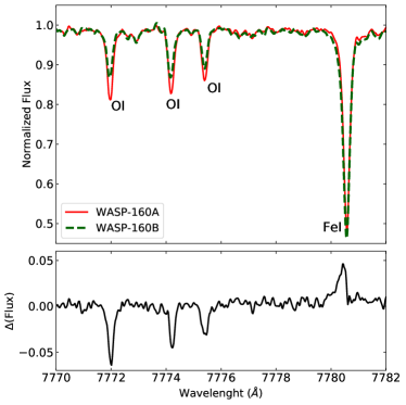
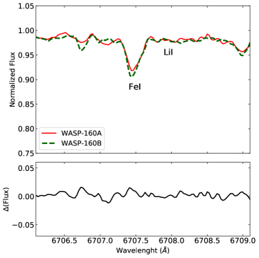
Figure 1: Top panels: spectra of WASP-160A (red solid) and WASP-160B (green dashed) around the oxygen triplet region (left) and the 6708 Å lithium line (right). Bottom panels: normalized flux difference between the WASP-160A and B.

2 Observations and literature data

In this section, we present the newly acquired observations and describe their data reduction. We also summarize all the data from the literature utilized in the global analysis of the WASP-160B system, including the following photometric and spectroscopic observations taken at ESO La Silla Observatory in Chile, already published in LE19:

• One partial transit observed in the I+z’-band the night of 16 Dec 2014 with the 0.6-m TRAPPIST telescope.

• One complete and one partial transit observed the nights of 26 Dec 2015 and 02 Jan 2017, respectively, in the r’-band with the EulerCam at the 1.2-m Euler-Swiss telescope.

• 30 radial velocities (RV) obtained with the CORALIE echelle spectrograph at the 1.2-m Euler-Swiss telescope.

2.1 High-resolution Spectroscopy

We observed WASP-160A and WASP-160B on 2019 November 13 UT with the Gemini Remote Access to CFHT ESPaDOnS Spectrograph (GRACES; Chene et al., 2014) at the 8.1-m Gemini North telescope. Observations were carried out in the queue mode (GN-2019B-Q-116, PI: E. Jofré) in the one-fiber mode (object only), which achieves a resolving power of R$\sim$ 67,500 between 400 and 1,050 nm. We obtained consecutive exposures of 4 $\times$ 1060 s for WASP-160A and 4 $\times$ 1469 s for WASP-160B.

These observations along with a series of calibrations including 6 $\times$ ThAr arc lamp, 10 $\times$ bias, and 7 $\times$ flat-field exposures were used as input in the OPERA (Open source Pipeline for ESPaDOnS Reduction and Analysis) code software (Martioli et al., 2012) to obtain the reduced data. The reduction details can be found in Jofré et al. (2020). Briefly, the reduction includes optimal extraction of the orders, wavelength calibration, and normalization of the spectra.

Using the IRAF task scombine, the individual exposures of each target were co-added to obtain the final spectra which present a signal-to-noise ratio per resolution element of S/N $\sim$ 350 and S/N $\sim$ 320 around 6000 Å, for WASP-160A and WASP-160B, respectively. We derived absolute radial velocities (RVs) by cross-correlating our program stars with standard stars using the IRAF task fxcor, obtaining VR = $-$6.28 $\pm$ 0.03 km s^-1 for the primary and VR = $-$6.30 $\pm$ 0.06 km s^-1 for the secondary. These values are in excellent agreement with the absolute RVs from Gaia Data Release 2 (DR2; Gaia Collaboration et al., 2018) and those from LE19. The combined spectra were corrected for the RVs shifts with the IRAF task dopcor. Small portions of the WASP-160A and WASP-160B final spectra are shown in Figure 1.

For the spectroscopic analysis below, we also employed a solar spectrum (reflected sunlight from the Moon) obtained with the same GRACES setup (SNR $\sim$ 410 at 6000 Å) but observed on a different date. Although this is not ideal, given that the components of the binary system are not solar twins (see Section 3.1), the highest precision in the chemical abundances is obtained from the differential analysis between WASP-160A and B as we show in Section 3.1.

2.2 Time-series Photometric Observations

In order to refine the planetary parameters of WASP-160B b, we obtained six new full transits: one of them was observed by our team with the FRAM telescope and the other five were observed by the Transiting Exoplanet Survey Satellite (TESS; Ricker, 2015).

2.2.1 FRAM

One full transit of WASP-160B b was observed in the R-filter the night of 2020 February 19 with the 0.3-m FRAM (F/(Ph)otometric Robotic Atmospheric Monitor) telescope, which is part of the Pierre Auger Observatory in Argentina. FRAM is a 0.3-m Orion Optimised Dall-Kirkham, f/6.8 with Moravian Instruments CCD MII G4-16000, 4096$\times$4096 pixels, and a field of view of 62′$\times$62′, and photometric BVRI filters (Janeček et al., 2019). At the end of the night, we took dark and sky-flat frames. A master dark was subtracted from the 124 science images and then divided by a master flat created as the median combined dark-corrected individual sky-flats using standard IRAF routines. As in Petrucci et al. (2020), we used the FOTOMCAp code (Petrucci & Jofré, 2016) to measure precise instrumental magnitudes and then selected three non-variable stars in the field as comparisons to build up the differential light curve with the lowest dispersion in magnitudes.

In order to choose the best detrending model to the photometric data, we first subtracted a JKTEBOP (Southworth et al., 2004) transit model from the resulting observed light curve. This transit model was computed by fixing the inclination, sum and ratio of the relative planetary and stellar radii, and limb-darkening coefficients to the values determined by LE19. Airmass, background counts, FWHM, spatial shifts (in X and Y), peak-value, and seeing were measured for each timestamp. We created different detrending models as linear combinations of these variables and fitted the residuals. The final adopted light curve of WASP-160B (Figure 11) was the light curve corrected by the model that minimized the chi-square of the residuals, in this case, the one that combined all the 7 variables.

2.2.2 TESS

WASP-160AB was observed by TESS with 30-min-cadence in sector 6 (2018 December 11 to 2019 January 07). These data, publicly available in the form of full frame images (FFI), were analyzed with the tools provided by the Lightkurve Python package (Lightkurve Collaboration et al., 2018). We performed single aperture photometry on the 987 available FFI, only considering the square pixel with the highest flux value centered on the planet host-star, WASP-160B (Figure 2). To remove the systematics owing to scattered light and spacecraft instrument/motion noise, we applied a Savitzky-Golay filter (Savitzky & Golay, 1964) provided by Lightkurve that, basically, smooths the light curve by fitting a polynomial at consecutive intervals. In Figure 12, we present the final phase folded-transit light curve of WASP-160B considering the five individual transits found in the sector 6 of TESS.

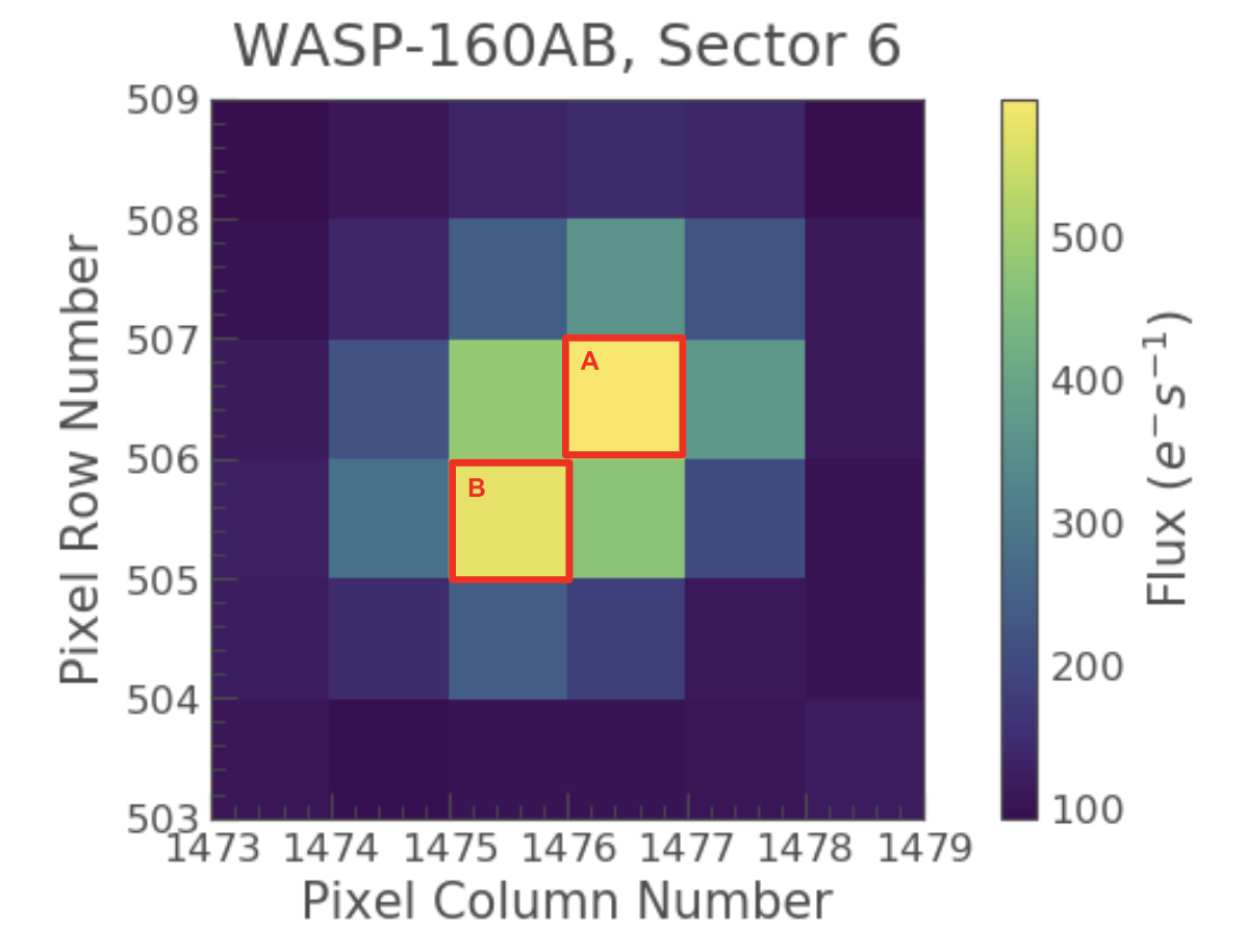
Figure 2: 6$\times$6 pixel TESS FFI centered on WASP-160AB. Light and dark colors show pixels with high and low flux values, respectively. Red squares and letters indicate the pixels selected to perform the aperture photometry of both stars (see the text for details).

Given that the size of the TESS pixel is 21 arcsec and the separation between the components of the system is $\sim$28 arcsec, the selected aperture includes the flux contribution of both stars. This light contamination from a blended stellar source makes the measured transit depth shallower than it truly is. In order to avoid a wrong determination of the planetary radius, we fitted a parameter that takes into account this effect during the light curve modeling as is explained in Section 5.2. This allowed us to correctly estimate the radius of the planet from the TESS data.

3 Stellar Characterization

3.1 Spectroscopic Fundamental Parameters

The atmospheric parameters T_eff (effective temperature), $\log g$ (surface gravity), [Fe/H] (abundance of iron), and $v_{micro}$ (microturbulent velocity) were derived from equivalent widths (EWs) of iron lines by imposing differential excitation and ionization equilibrium, as described in previous works (e.g., Ramírez et al., 2015, 2019; Saffe et al., 2015, 2017). Briefly, in this method, the T_eff and $v_{micro}$ are iteratively modified until the correlation of differential iron abundance (Fe i lines only) with excitation potential (EP=$\chi$) and reduced equivalent width (REW = $\log\mathrm{EW}/\lambda$), respectively, are minimized. Simultaneously, $\log g$ is modified until the differential abundance derived from Fe i lines approaches to the one computed from Fe ii lines. To perform this process automatically, we employed the Qoyllur-Quipu (or q²) Python package (Ramírez et al., 2014), which uses the MOOG code (Sneden, 1973) to translate the EW measurements into abundances via the curve-of-growth method. In addition, q² uses linearly interpolated one-dimensional local thermodynamic equilibrium (LTE) Kurucz ODFNEW model atmospheres (Castelli & Kurucz, 2003).

The iron line list, as well as the atomic parameters (EP and oscillator strengths, $\log gf$), were compiled from Ramírez et al. (2015) and the EWs were manually measured by fitting Gaussian profiles using the splot task in IRAF. To make a precise and consistent measurement of the EWs in the spectra of WASP-160A, WASP-160B and the Sun, for each line, we carefully selected the same continuum region line by overplotting the spectra of the stars.

Figure 3: Line-by-line iron abundance of WASP-160B, computed relative to WASP-160A, as a function of excitation potential (upper panel), reduced EW (middle panel), and wavelength (bottom panel). Blue crosses (green circles) correspond to Fe i (Fe ii) lines. In the top and middle panel, solid lines are linear fits to the Fe i data, while the solid black line in the bottom panels indicates the average iron abundance from all lines.

We first performed the line-by-line differential analysis of both components of the stellar pair using our solar spectrum as reference, adopting as solar parameters T_eff = 5777 K, $\log g$ = 4.44 dex, [Fe/H] = 0 dex, and $v_{micro}$ = 1.0 km s^-1. As initial values we employed those obtained by LE19, which are included in the first block of Table 1. The results of this computation are listed in the second block of Table 1. We note that only the [Fe/H] value for WASP-160A and the T_eff of WASP-160B computed by LE19 are consistent, within the error bars, with our results. The rest of the parameters agree only within the 2$\sigma$ range. In particular, the $\log g$ and [Fe/H] values are systematically larger than ours. The discrepancies are likely related to the use of different techniques (i.e., differential vs. absolute), models of stellar atmospheres, line-lists and atomic data, and the use of spectra of different quality (e.g., Bedell et al., 2014; Hinkel et al., 2016; Jofré et al., 2017, 2020).

From our first differential results (second block of Table 1), we observe that both components present very similar $\log g$ and [Fe/H] values ($\Delta\log g\sim 0.02$ dex and $\Delta$[Fe/H] $\sim$ 0.02 dex). The WASP-160 stellar components present a difference in effective temperature of $\Delta$T_eff $\sim$ 200 K, which after the system HD 20781/82 with $\Delta$T_eff $\sim$ 465 K (Mack et al., 2014), is the stellar pair with the largest difference in T_eff among the sample of binaries hosting planetary systems with high-precision chemical abundances (e.g., Ramírez et al., 2019). Even with the large difference in T_eff, the components of the WASP-160 binary system can still be considered as twin stars according to the criteria of Nagar et al. (2020, $\Delta$T_eff $\lesssim$ 300 K and $\Delta$$\log g$ $\lesssim$ 0.2 dex). The measured $\Delta$T_eff might account for the slightly larger errors in the derived fundamental parameters, especially the abundances of iron (and other elements), in comparison with previous differential analysis of stellar twins (Ramírez et al., 2015; Teske et al., 2016a; Saffe et al., 2017). In Section 4.2, we discuss the impact of the derived T_eff on the abundance differences between the binary components.

Table 1: Atmospheric parameters of WASP-160A and WASP-160B

Star	$T_{\mathrm{eff}}$	$\log g$	$\mathrm{[Fe/H]}$	$v_{\mathrm{micro}}$
	(K)	(cgs)	(dex)	(km $s^{-1}$)
Lendl et al. (2019)
WASP-160A	5300 $\pm$ 100	4.50 $\pm$ 0.20	0.19 $\pm$ 0.09	$-$
WASP-160B	5300 $\pm$ 100	4.60 $\pm$ 0.10	0.27 $\pm$ 0.10	$-$
$\Delta$(B$-$A)	0 $\pm$ 141	0.10 $\pm$ 0.22	0.08 $\pm$ 0.13	$-$
This work, solar reference (Section 3.1)
WASP-160A	5424 $\pm$ 16	4.42 $\pm$ 0.05	0.139 $\pm$ 0.017	0.91 $\pm$ 0.06
WASP-160B	5218 $\pm$ 18	4.44 $\pm$ 0.05	0.149 $\pm$ 0.020	0.76 $\pm$ 0.09
$\Delta$(B$-$A)	$-$206 $\pm$ 24	0.02 $\pm$ 0.07	0.01 $\pm$ 0.026	$-$0.15 $\pm$ 0.11
This work, WASP-160A reference (Section 3.1)
WASP-160A	5424 $\pm$ 16	4.42 $\pm$ 0.05	0.139 $\pm$ 0.017	0.91 $\pm$ 0.06
WASP-160B	5215 $\pm$ 4	4.47 $\pm$ 0.02	0.151 $\pm$ 0.004	0.75 $\pm$ 0.03
$\Delta$(B$-$A)	$-$209 $\pm$ 16	0.05 $\pm$ 0.05	0.012 $\pm$ 0.017	$-$0.16 $\pm$ 0.07

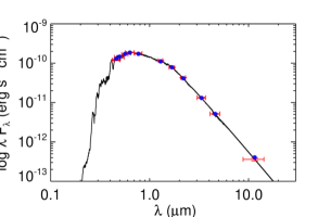
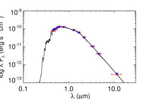
Figure 4: Spectral energy distributions of WASP-160A (left) and WASP-160B (right). The red points represent the measurements of the fluxes in the WASP-160 stars in the optical, NIR, and mid-IR passbands listed in Table 2. The vertical bars are the $1\sigma$ photometric uncertainties and the horizontal error bars indicate the width of the photometric bandpasses. Blue symbols are the model fluxes from the best-fit NextGen atmosphere model (black).

On the other hand, it can also be noticed that WASP-160A and WASP-160B are significantly different from the Sun in terms of T_eff (i.e, non-solar twins) and therefore it would be expected to obtain more precise parameters by comparing the two stars differentially to each other. Hence, we repeated the process to measure the stellar parameters of WASP-160B but considering the star WASP-160A as reference by adopting its solar-reference parameters derived above as fixed. We choose WASP-160A as the reference star since its solar-relative atmospheric parameters (especially the T_eff) are more similar to those of the Sun and therefore expected to be more reliable than those of the B component (see Teske et al., 2016a). The final result (WASP-160B $-$ WASP-160A) is shown in Figure 3 and the derived parameters with their errors are listed in the last block of Table 1. As expected, the atmospheric parameters of WASP-160B are almost the same than those computed using the Sun as reference, but the errors are considerably smaller. These errors correspond to intrinsic uncertainties of the method and are estimated as in Epstein et al. (2010) and Bensby et al. (2014). Both the results derived comparing the WASP-160 stars to the Sun and those obtained through a strict differential analysis of WASP-160B relative to WASP-160A reveal that the B component is only marginally iron-enhanced relative to A by $\sim$+0.01 dex.

Table 2: Stellar properties of WASP-160A and WASP-160B

Parameter	WASP-160A	WASP-160B	Source
Astrometry and kinematics
Proper motion in RA, $\mu_{\alpha}$ (mas yr-1)	26.854 $\pm$ 0.034	26.975 $\pm$ 0.030	Gaia DR2
Proper motion in DEC, $\mu_{\delta}$ (mas yr-1)	$-$34.821 $\pm$ 0.042	$-$34.830 $\pm$ 0.037	Gaia DR2
Parallax, $\pi$ (mas)	3.38 $\pm$ 0.06	3.36 $\pm$ 0.06	Gaia DR2
Barycentric radial velocity, RV (km $s^{-1}$)	$-$6.28 $\pm$ 0.03	$-$6.30 $\pm$ 0.06	This work (Sec. 2.1)
Space velocity component, U (km $s^{-1}$)	$-$6.57 $\pm$ 0.02	$-$6.59 $\pm$ 0.03	This work (Sec. 3.4)
Space velocity component, V (km $s^{-1}$)	2.96 $\pm$ 0.02	2.97 $\pm$ 0.04	This work (Sec. 3.4)
Space velocity component, W (km $s^{-1}$)	1.05 $\pm$ 0.01	1.06 $\pm$ 0.03	This work (Sec. 3.4)
Galaxy population membership	Thin disk	Thin disk	This work (Sec. 3.4)
Photometry
B (mag)	13.452 $\pm$ 0.040	13.983 $\pm$ 0.030	APASS
V (mag)	12.677 $\pm$ 0.020	13.094 $\pm$ 0.020	APASS
$g^{\prime}$ (mag)	13.014 $\pm$ 0.020	13.500 $\pm$ 0.030	APASS
$r^{\prime}$ (mag)	12.426 $\pm$ 0.020	12.820 $\pm$ 0.020	APASS
$i^{\prime}$ (mag)	12.253 $\pm$ 0.030	12.595 $\pm$ 0.020	APASS
J (mag)	11.300 $\pm$ 0.030	11.591 $\pm$ 0.030	2MASS
H (mag)	10.937 $\pm$ 0.020	11.172 $\pm$ 0.020	2MASS
Ks (mag)	10.831 $\pm$ 0.020	11.055 $\pm$ 0.020	WISE
$W_{1}$ (mag)	10.789 $\pm$ 0.030	11.021 $\pm$ 0.030	WISE
$W_{2}$ (mag)	10.834 $\pm$ 0.030	11.067 $\pm$ 0.030	WISE
$W_{3}$ (mag)	10.798 $\pm$ 0.092	11.038 $\pm$ 0.110	WISE
V-band extinction, AV (mag)	0.0308 $\pm$ 0.015	0.0308 $\pm$ 0.0015	Schlafly & Finkbeiner (2011)
Adopted atmospheric and physical parameters
Effective temperature, $T_{\mathrm{eff}}$ (K)	5424 $\pm$ 16	5215 $\pm$ 4	This work (Sec. 3.1)
Surface gravity, $\log g$ (cgs)	4.42 $\pm$ 0.05	4.47 $\pm$ 0.02	This work (Sec. 3.1)
Metallicity, $\mathrm{([Fe/H])}$	0.139 $\pm$ 0.017	0.151 $\pm$ 0.004	This work (Sec. 3.1)
Microturbulent velocity, $v_{\mathrm{micro}}$ (km $s^{-1}$)	0.91 $\pm$ 0.06	0.75 $\pm$ 0.03	This work (Sec. 3.1)
Macroturbulent velocity, $v_{\mathrm{macro}}$ (km $s^{-1}$)	4.51 $\pm$ 0.032	4.83 $\pm$ 0.025	This work (Sec. 3.1)
Rotational velocity, $v\sin i$ (km $s^{-1}$)	3.96 $\pm$ 0.30	3.61 $\pm$ 0.48	This work (Sec. 3.1)
Activity index $\log R^{\prime}_{HK}$	$-$4.714 $\pm$ 0.0434	$-$4.766 $\pm$ 0.0434	This work (Sec. 4.3)
Mass, $M_{\mathrm{\star}}$ ($M_{\mathrm{\odot}}$)	0.926 ${}^{+0.024}_{-0.022}$	0.879 ${}^{+0.022}_{-0.020}$	This work (Sec. 3.3)
Radius, $R_{\mathrm{\star}}$ ($R_{\mathrm{\odot}}$)	0.950 ${}^{+0.018}_{-0.019}$	0.872 ${}^{+0.013}_{-0.012}$	This work (Sec. 3.3)
Age, $\tau$ (Gyr)	8.0 ${}^{+2.5}_{-2.6}$	8.2 ${}^{+2.8}_{-3.0}$	This work (Sec. 3.3)
Luminosity, $L_{\mathrm{\star}}$ ($L_{\mathrm{\odot}}$)	0.69 $\pm$ 0.026	0.502 ${}^{+0.015}_{-0.014}$	This work (Sec. 3.3)
Density, $\rho_{\mathrm{\star}}$ (cgs)	1.522 ${}^{+0.11}_{-0.099}$	1.869 ${}^{+0.095}_{-0.088}$	This work (Sec. 3.3)

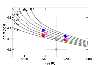
Figure 5: Locations of WASP-160A (squares) and WASP-160B (circles) in the T_eff–$\log g$ plane using different sets of parameters. The blue symbols show the purely differential spectroscopic parameters derived in this work. The pink symbols represent T_eff and $\log g$ values derived from the global analysis performed with EXOFASTv2. Those in red indicate the spectroscopic T_eff combined with the trigonometric $\log g$ obtained with q². Green symbols correspond to the location of both stars with the parameters of LE19. The solid lines mark Yonsei-Yale isochrones of the noted ages for [Fe/H] = 0.15 dex.

Additionally, we derived projected rotational velocities (v$\sin i$) based on the spectral synthesis of relatively isolated iron lines, as is detailed in Jofré et al. (2020). In this case, however, we adopted the calibration of Valenti & Fischer (2005) to determine macroturbulence. We find that both objects have similar low velocities: v$\sin i$ = 3.96 $\pm$ 0.30 km s^-1 and v$\sin i$ = 3.61 $\pm$ 0.48 km s^-1, for WASP-160A and B, respectively.

3.2 Consistency checks on T_eff

To check the reliability of the derived spectroscopic T_eff values, we performed a series of independent tests. First, we computed photometric temperatures for both stars using the metallicity-dependent T_eff-color calibrations formulae by Casagrande et al. (2010) using our highest precision [Fe/H] values from Table 1 and the ($B-V$), ($V-J$), ($V-H$), ($V-K_{S}$), and ($J-K_{S}$) colors calculated from the photometric data listed in Table 2. The average resulting values are T_eff = 5393 $\pm$ 45 K for WASP-160A and T_eff = 5179 $\pm$ 58 K for WASP-160B, which not only are in good agreement with the spectroscopic determinations but also keep a similar $\Delta$T_eff value.

As another test, we computed T_eff from EWs line strength ratios using the T_eff-LR code as described in Jofré et al. (2020). In excellent agreement with the results from the differential spectroscopic analysis, we obtained T_eff = 5400 $\pm$ 16 K for WASP-160A and T_eff = 5208 $\pm$ 18 K for WASP-160B. We also obtained T_eff from the analysis of the Spectral Energy Distribution (SED) based on the latest version of the Virtual Observatory SED Analyzer (VOSA, Bayo et al., 2008) as detailed in Jofré et al. (2020). The effective temperatures computed from VOSA are T_eff = 5400 $\pm$ 50 K and T_eff = 5200 $\pm$ 60 K for the components A and B, respectively, which once again are consistent with our spectroscopic estimates.

3.3 Stellar mass, radii, and ages

Following Ramírez et al. (2014), we derived stellar mass M_⋆, radius R_⋆, and ages $\tau_{\mathrm{\star}}$ using probability distribution functions with Yonsei-Yale (YY) stellar evolution models (Demarque et al., 2004). This was carried out via the q² pipeline, which has been extensively tested in the literature (e.g., Ramírez et al., 2014; Meléndez et al., 2017; Bedell et al., 2017; Liu et al., 2020). As input, we used Gaia DR2 parallaxes (Gaia Collaboration et al., 2018), V magnitudes, and the spectroscopic T_eff and [Fe/H] values derived above (third block of Table 1). For WASP-160A, this code returned M_⋆ = 0.946 $\pm$ 0.018 M_⊙, R_⋆ = 0.934 $\pm$ 0.020 R_⊙, and $\tau_{\star}$= 6.067 $\pm$ 1.689 Gyr, whilst for WASP-160B, we found M_⋆ = 0.881 $\pm$ 0.014 M_⊙, R_⋆ = 0.860 $\pm$ 0.014 R_⊙, and $\tau_{\star}$= 7.440 $\pm$ 1.597 Gyr. This code also provides the trigonometric gravities, which allow us to perform a consistency check on the spectroscopic $\log g$ values. q² yields $\log g$ = 4.472 $\pm$ 0.026 dex and $\log g$ = 4.513 $\pm$ 0.021 dex for WASP-160A and B, respectively. Both values are in agreement, within the errors, with the estimates found from the spectroscopic equilibrium.

We also derived M_⋆, R_⋆, and $\tau_{\mathrm{\star}}$ of both stars using the EXOFASTv2 software package (Eastman et al., 2013, 2019). Here, the stellar models are simultaneously constrained by our newly derived effective temperature and metallicity from Table 1, the SED constructed from the catalog broadband photometry (see Table 2 and Figure 4), the Gaia DR2 parallax (also in Table 2; Gaia Collaboration et al., 2018), and extinction in the direction of WASP-160 (A_V = 0.0308 $\pm$ 0.0015 mag; Schlafly & Finkbeiner, 2011). We set Gaussian priors for the parameters for which we have independent constraints, namely the T_eff, [Fe/H], parallax and extinction, with widths corresponding to their one-sigma uncertainties. We set an upper limit to the extinction of 0.04 to avoid unrealistic solutions. Additionally, we used as starting points in $\log{g}$, M_⋆, R_⋆, and $\tau_{\mathrm{\star}}$, the values derived with q², and since they are not independently constrained, we do not restrict them in the fitting. The stellar physical properties are then derived by simultaneously fitting a single star SED and either MIST (Choi et al., 2016) or YY stellar models. For WASP-160B, an additional constraint is provided by the stellar density derived from the transit light curve data (see Section 5). Thus, this code also allows us to make a consistency check both on the spectroscopic T_eff and $\log g$ derived above. Using the YY models, for WASP-160A EXOFASTv2 returned T_eff = 5396 $\pm$ 19 K, $\log g$ = 4.449 $\pm$ 0.023 dex, M_⋆ = 0.926 ${}^{+0.024}_{-0.022}$ M_⊙, R_⋆ = 0.950 ${}^{+0.018}_{-0.019}$ R_⊙, and $\tau_{\star}$= 8.0 ${}^{+2.5}_{-2.6}$ Gyr, whilst for WASP-160B, we found T_eff= 5202 $\pm$ 15 K, $\log g$ = 4.501 $\pm$ 0.016 dex, M_⋆ = 0.879 ${}^{+0.022}_{-0.020}$ M_⊙, R_⋆ = 0.872 ${}^{+0.013}_{-0.012}$ R_⊙, and $\tau_{\star}$= 8.2 ${}^{+2.8}_{-3.0}$ Gyr. These values are almost identical to those obtained using the MIST grids and, moreover, they are in excellent agreement with those from q².

As final values of mass, radii, and ages we adopted the results provided by EXOFASTv2 which are listed in Table 2. Here, we also have included the adopted differential atmospheric parameters, which for WASP-160A are those using the Sun as reference whilst the parameters for WASP-160B are relative to WASP-160A (third block of Table 1).

The small difference between the spectroscopic $\log g$ and T_eff values and those derived using photometry and parallax information, all within 1$\sigma$, can be seen in Figure 5. Here we plot the locations of both stars on the T_eff versus $\log g$ diagram, along with YY theoretical isochrones. Assuming that the stars are bound and coeval, their ages should be consistent and fall approximately on the same isochrone. Our spectroscopic $\log g$ values would make both stars slightly older than $\sim$ 9 Gyr, whilst if we consider the position given by the trigonometric $\log g$ values and our spectroscopic T_eff obtained with q², both stars are located over the 6–7 Gyr isochrones. For the results derived from the EXOFASTv2, the stars fall on the same $\sim$ 8 Gyr isochrone. However, given the obtained uncertainties, all ages would be consistent with those of thin disk stars ($\lesssim$9 Gyr, e.g., Bernkopf et al., 2001; Nissen, 2004; Kilic et al., 2017), which is in agreement with the Galaxy population membership derived for the stars in Section 3.4. As we will see later in Section 4.1, the small difference in the $\log g$ values does not affect our relative abundance ratios in any significant way. In agreement with the location of both stars on the T_eff - $\log g$ plane, based on the calibration of Pecaut & Mamajek (2013) and our derived stellar parameters, we estimated that WASP-160A and WASP-160B would correspond to G8 and K0.5 dwarf stars.

The only previous estimations of stellar mass, radius, and age for the WASP-160 stars were reported by LE19. They used their spectroscopic fundamental parameters, the stellar density derived from the transit light curve (only for WASP-160B), Gaia photometry, and the distance as initial constraints to obtain stellar masses, radii, and ages through PARSEC stellar evolution models (Bressan et al., 2012). All the parameters agree with our results within the errors.

3.4 Elemental abundances

Adopting the spectroscopic atmospheric parameters presented in the third block of Table 1 as the first choice, we measured the abundances of 25 elements other than iron for the WASP-160 stars. The abundances were derived from EWs using the curve-of-growth approach with the MOOG code (abfind driver) via the q² code. The EWs were measured following the same procedure employed for the iron lines (see Section 3.1). The line list and atomic parameters adopted were taken from Ramírez et al. (2014) and Meléndez et al. (2014). We also included near-IR lines for C from Amarsi et al. (2019) and for N from Takeda et al. (2001) and Ecuvillon et al. (2004). The abundances of Sc, Ti, and Cr (in addition to Fe) were obtained from both neutral and singly-ionized species, whilst for Y, Zr, Ba, and Eu only singly-ionized species are available. For the rest of the elements, only neutral species were used. Hyperfine splitting was taken into account for V, Mn, Co, Cu, Rb, Y, Ba and Eu. The O abundance was computed from the 7771-5 Å IR triplet, adopting the non-LTE corrections by Ramírez et al. (2007). The line list and atomic parameters used in this work along with the EWs measured in the WASP-160 stars and our solar spectrum are listed in Table 3 of the Appendix A. The line-by-line differential abundances relative to solar ([X/H]) and those using WASP-160A as the reference star ($\Delta$[X/H]_B-A), along with the errors, are listed in Table 4 (Appendix A). These errors are computed adding in quadrature both the line-to-line scatter and the errors propagated from each parameter uncertainty as in Ramírez et al. (2015). Our errors in relative abundances, $\Delta$[X/H]_B-A, vary from one species to another in the 0.005–0.030 dex range. In particular, the median error is 0.017 dex and 0.008 dex for elements with T_c $\lesssim$ 900 K and for those with T_c $>$ 900 K, respectively.

In both stars the lithium line (Li i) at 6707.8 Å is not detected (Figure 1, right) and therefore we can only derive an upper limit of A(Li) $\lesssim$ 0.17 dex and A(Li) $\lesssim$ 0.6 dex for WASP-160A and B, respectively, by performing a synthesis analysis. This result is in agreement with the non-detection of lithium reported by LE19 for WASP-160B, and supports the relatively old ages derived in Section 3.3. The low abundance of lithium also might be caused by the relatively low temperature of WASP-160A and B since stars with T_eff below 5500 K have A(Li) $\lesssim$ 0.5 dex (Ramírez et al., 2011; Aguilera-Gómez et al., 2018), as a consequence of having deeper convective zones.

Considering the relatively old age of the WASP-160 stars, we determined their Galactic population membership. First, following the procedure detailed in Jofré et al. (2015), we derived the Galactic space-velocity components (U, V, W) listed on Table 2 using the radial velocities measured from the GRACES spectra and the proper motions and parallaxes from Gaia DR2. From these space-velocity components and the membership formulation by Reddy et al. (2006), we found that the probability of belonging to the thin disk population is $\sim$99% for both stars. The $\alpha$-elemental abundances of WASP-160A ([$\alpha$/Fe]= 0.02 dex) and WASP-160B ([$\alpha$/Fe]= 0.04 dex) appear to be consistent with the kinematic thin-disk membership of the system.

Strictly speaking the components of the WASP-160 stellar pair, with consistent astrometry and near-identical systemic RVs, are by definition comoving stars and, in principle, there is no guarantee that they are gravitationally bound (see e.g., Oh et al., 2017; Simpson et al., 2019; Ramírez et al., 2019). However, their chemical compositions along with their same old ages ($\sim$8 Gyr), which are rare for thin disk objects, suggest that a lucky alignment of these two comoving stars or a capture scenario is unlikely. Moreover, following Andrews et al. (2017) and Ramírez et al. (2019), we examined the location of the WASP-160 pair in the plot of projected separation versus total velocity difference (see Fig. 7 in Ramírez et al., 2019). With a projected separation of $s$ = 8060 AU between the components ($\log s$ = 3.90 AU) and a difference in total velocity of $\Delta V$ = 0.02 km $s^{-1}$ ($\log\Delta V$ $\sim$ $-$1.70 km $s^{-1}$), WASP-160 fall safely within the limits where a system can be considered as physically bound and hence a true binary.

4 Chemical differences between WASP-160A and B

Figure 6 shows the derived differential abundances of WASP-160B relative to WASP-160A, $\Delta$[X/H]_B-A, as a function of atomic number. We can see that WASP-160B is more metal-rich in almost all elements relative to its binary companion WASP-160A. Conservatively, if we exclude the abundances of those elements measured from only one line (i.e., K, Zn, Eu, and Zr), we find a weighted average (and weighted standard deviation) of $\Delta$[X/H]_B-A = 0.022 $\pm$ 0.006 dex (i.e., an excess detected at the $\sim$4$\sigma$ level). Hereafter, we discuss our results ignoring the K, Zn, Eu, and Zr abundances.

In Figure 7, we show the derived differential elemental abundances of WASP-160B relative to WASP-160A versus the 50% condensation temperature (T_c) from Lodders (2003) for solar-composition gas. The $\Delta$[X/H]_B-A seems to correlate with T_c, with the lowest values for the volatile elements like carbon around $\sim$$-$0.05 dex, and the highest up to $\sim$0.1 dex for vanadium, the refractory element with the highest T_c in our list. In particular, we note that the Saturn-mass planet-host star WASP-160B seems to be depleted in volatiles (elements with T_c $\lesssim$ 900 K), with a weighted average and standard deviation of $\Delta$[X/H]_B-A = $-$0.035 $\pm$ 0.008 dex (i.e., a deficiency detected at the 5$\sigma$ level) and enhanced in refractories (elements with T_c $>$ 900 K) with a weighted average and standard deviation of $\Delta$[X/H]_B-A = +0.033 $\pm$ 0.005 dex (i.e., an excess detected at the 7$\sigma$ level) relative to its companion WASP-160A. To date, no planet has been detected around WASP-160A.

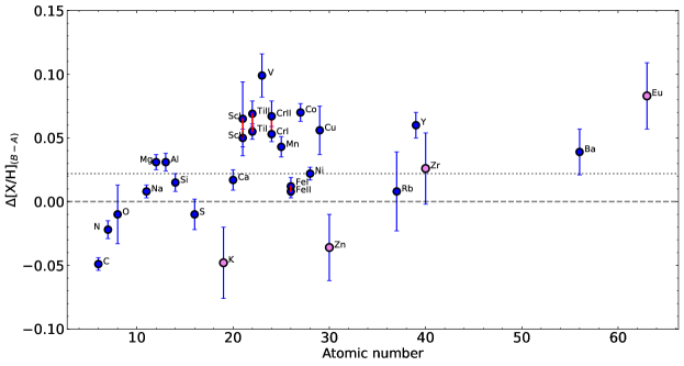
Figure 6: Elemental abundance differences between WASP-160B and WASP-160A as a function of atomic number. The dashed line corresponds to identical composition and the dotted line represents the weighted average of $\Delta$[X/H]_B-A considering all the elements but those measured from only one line (see text for more details). Red vertical lines connect two species of the same chemical element (e.g., Sc i and Sc ii) and pink circles show the species measured from one line only (K i, Zn i, Eu ii, and Zr ii).

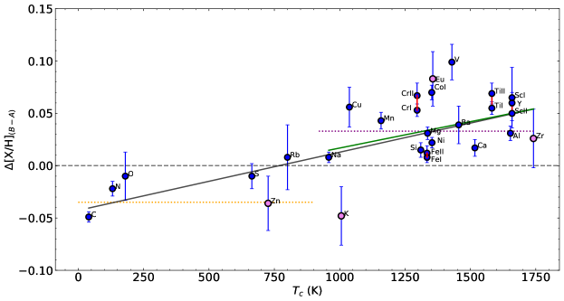
Figure 7: Chemical composition difference between WASP-160B and WASP-160A versus condensation temperature. The solid black and green lines are the weighted linear least-squares fit to all the elements and refractory elements measured from more than one line, respectively. The horizontal dotted orange and violet lines represent the weighted average for the volatile and refractory elements, respectively. As before, the dashed line corresponds to identical composition, and the solid red vertical lines connect two species of the same chemical element and pink circles show the species measured from one line only.

We tested three models on the $\Delta$[X/H]_B-A versus T_c data to investigate a possible correlation. First, a zero-slope ($m$=0) and zero-intercept fit ($b$=0; the black-dashed line in Figure 7) results in a $\chi_{r}^{2}$ value of 27.9, a mean scatter of $\sigma_{f}$= 0.033, and a Bayesian Information Criterion value of BIC = 699. Second, a weighted linear fit to the data with $m$=0 and free intercept gives $b$= 0.022 $\pm$ 0.006 dex with $\chi_{r}^{2}$ = 19.9, $\sigma_{f}$= 0.033, and BIC= 481. Finally, a weighted linear fit to the data with $m$ and $b$ as free parameters results in an intercept of $b$=$-$0.042 $\pm$ 0.004 dex and a positive slope of (5.56 $\pm$ 0.79) $\times 10^{-5}$ dex K^-1, with $\chi_{r}^{2}$ = 6.6, $\sigma_{f}$= 0.021, and BIC = 158. Considering the $\chi^{2}$, $\sigma_{f}$, and BIC values obtained for each model, we find that the linear fit with unconstrained slope and intercept provides the best fit to the data in comparison with the other two models.

Considering all elements (both volatiles and refractories), the analysis above supports a non-negligible slope for the $\Delta$[X/H]_B-A versus T_c data, with a significance of the slope at the $\sim$7$\sigma$ level. The Pearson’s r correlation test gives in this case a coefficient of r $\sim$ 0.76. Moreover, following Maldonado & Villaver (2016), we carried out 100,000 bootstrap Monte Carlo (MC) simulations to estimate the probability that uncorrelated random data sets could reproduce the observed trend in Figure 7, and hence the value of the slope. We found that this probability is only $\sim$4.6%, which gives additional support to a significant correlation between the differential abundances and T_c. If we only consider the behavior of the refractory elements, the data still favor a model with a non-zero positive slope over the other models. However, in this case, the slope of the weighted linear fit to refractory abundances versus T_c has a modest statistical significance ($\sim$2$\sigma$).

4.1 Impact of the Adopted Stellar Parameters

Teske et al. (2015) found that chemical differences between the stellar components of a binary system, and therefore the T_c trends, are sensitive to the chosen stellar parameters. Following the exercise presented in Ramírez et al. (2015, their Section 4.7), here we show how the $\Delta$[X/H]_B-A versus T_c trend observed in Figure 7 depends on the adopted fundamental parameters.

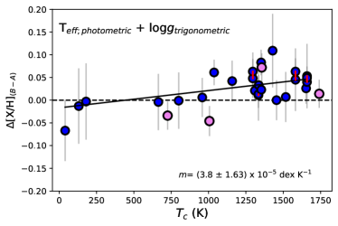
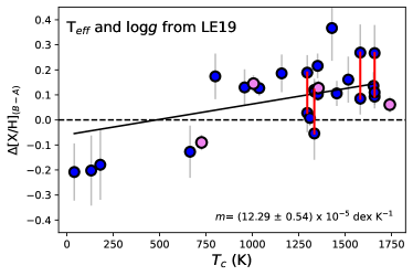
Figure 8: Same as in Figure 7, but using different choices of stellar parameters for WASP-160A and WASP-160B. The derived slope values of the fits are presented in the bottom-right corner of each panel.

Using our EWs measurements, we started by recomputing the $\Delta$[X/H]_B-A values using different sets of stellar parameters. First, we recalculated the abundances from our spectroscopic parameters of the WASP-160 stars computed using the Sun as reference for both stars (second block of Table 1). The abundances versus T_c correlation with this set of parameters, shown in the first panel of Figure 8, is very similar to the one obtained with our preferred set of parameters. Here, the offset of volatiles is $-0.033$ dex (weighted average) whilst the one for refractories is +0.035 dex. These values are very similar to those obtained using WASP-160A as reference. In this case, it is interesting to note that although the $\Delta$T_eff is basically the same (only 3 K smaller), a smaller $\Delta\log g$ of only 0.02 dex in comparison with a difference of 0.05 dex for the original parameters, does not produce a significant impact on the observed correlation.

The middle panel in Figure 8 shows the chemical pattern that results when we use the temperatures derived from photometric calibrations and the trigonometric $\log g$ values computed with q². Again, since the B$-$A relative parameters are the same in comparison with the previous case, a very similar and significant $\Delta$[X/H]_B-A versus T_c correlation is obtained although with a slightly smaller slope (3.8 $\pm$ 1.6 $\times 10^{-5}$ dex K^-1). Analogous results are obtained using the T_eff and $\log g$ values derived from EXOFASTv2 (not plotted).

The bottom panel shows the abundances derived using the parameters from LE19, which are listed in the first block of Table 1. In this case, as we mentioned in Section 3.1, there is a relatively discrepancy between our stellar parameters and those derived by LE19, but more importantly a larger difference in the B$-$A relative parameters. In particular, LE19 suggest $\Delta$T_eff = 0 K, $\Delta\log g$ = 0.05 dex, and $\Delta$[Fe/H] = 0.08 dex whilst for our preferred set we find $\Delta$T_eff= 209 K, $\Delta\log g$=0.05 dex, and $\Delta$[Fe/H] = 0.012 dex. Using the parameters of LE19, the offset between volatiles and refractories seems larger and, hence, causes a steeper correlation. However, the scatter is larger than the observed with the other choice of parameters. Moreover, with these parameters, the abundances of elements obtained from both neutral and singly-ionized species (e.g., Fe, Ti, Cr, Sc, indicated with red lines) show the largest differences in comparison with those obtained with other sets of parameters. For example, the difference $\Delta$[Ti i/H]_B-A $-$ $\Delta$[Ti ii/H]_B-A is 0.184 dex in this case, but we find a difference of $-$0.014 dex with our parameters. Based on these results, we consider that our derived stellar parameters are more accurate than those presented by LE19 (see also, Ramírez et al., 2015).

4.2 Effect of $\Delta$T_eff

In the same manner as Ramírez et al. (2015, see their Figure 8) and Saffe et al. (2017), here we explore how different our T_eff values ($\Delta$T_eff in particular) should be to completely blur the T_c trend and/or flip the sign of the slope.

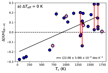
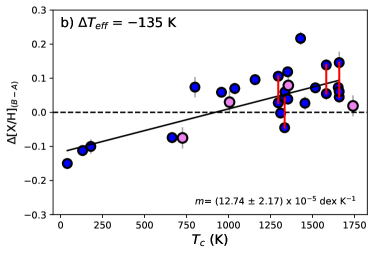
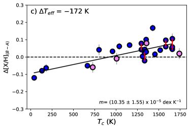
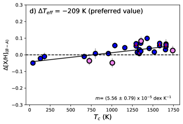
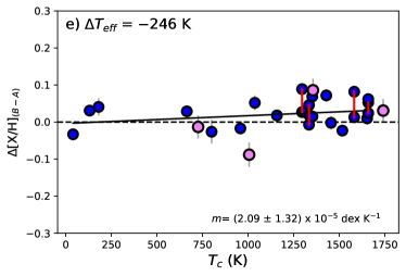
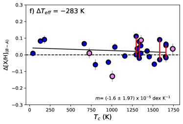
Figure 9: Same as in Figure 7, but considering different values of the B–A temperature difference, $\Delta$T_eff and keeping all other parameters constant. In this case, the panel with $\Delta$T_eff = $-$209 K is the same as Figure 7. The derived slope values of the fits are presented in the bottom-right corner of each panel.

In Figure 9 we show the abundances $\Delta$[X/H]_B-A that result considering different values of $\Delta$T_eff (from $-$283 K to $-$135 K) in the sense B$-$A. Here, only the effective temperature difference is changed by altering the temperature of the WASP-160B, while all the other parameters are kept constant.

Starting from our preferred values in panel (d), we note that the $\Delta$[X/H]_B-A versus T_c correlation becomes steeper, and also noisier, as the $\Delta$T_eff value decreases (see panel c, b, and a). Moreover, the abundance differences for elements with neutral and singly-ionized species available (Fe, Cr, Ti, Sc) increases (see the filled circles connected by red vertical lines). This behavior reaches a maximum considering, as an additional case, that the two stars are twins in terms of T_eff (i.e., $\Delta$T_eff = 0 K), which is very similar to the observed result when using the parameters of LE19. Thus, the large difference between the T_eff of the components of the WASP-160 system could not lead by itself to the observed T_c trend since the change in the slope goes in the opposite direction, i.e, as the stars become more similar in T_eff the T_c correlation is steeper.

Analyzing the behavior of the T_c trend at larger values of $\Delta$T_eff (i.e., less similar stars) beyond the preferred value can help us to explore when the correlation becomes marginal and/or changes its sign. Panels (e) and (f) in Figure 9 show the results when we derive the abundances considering $\Delta$T_eff values of $-$246 K and $-$283 K. Again, it can be noticed that as we move away from our preferred value, the difference between the abundances of elements derived from both neutral and singly-ionized species increases.

In particular, for the $\Delta$T_eff= $-$283 K we find that the trend shows a slightly negative slope whilst for $\Delta$T_eff= $-$246 K the trend exhibits a less steep slope (2.09 $\pm$ 1.32 $\times 10^{-5}$ dex K^-1 ) and, moreover, a linear fit with free values of $m$ and $b$ is no longer preferred against one with zero slope and free intercept. Nevertheless, in these two cases, WASP-160B remain chemically enhanced compared with WASP-160A. Moreover, for $\Delta$T_eff= $-$246 K, WASP-160B is still enhanced (by $\sim$ 0.007 dex at the 3$\sigma$ level) relative to WASP-160A and the trend is still present but modest statistical significant ($\sim$2$\sigma$) when considering only refractories.

To reach $\Delta$T_eff of $\sim$$-$246 K, it would be required that simultaneously the T_eff of WASP-160A be overestimated and that of WASP-160B be underestimated almost by 2$\sigma$. However, in addition to the behavior of the abundances of elements derived from both neutral and singly ionized lines, the excellent agreement between the spectroscopic $\Delta$T_eff value and those derived from independent techniques, gives us no reason to assume that our $\Delta$T_eff is different from the preferred and adopted one.

For these two last cases, and especially for that of $\Delta$T_eff = $-$246 K, one might still wonder if exists a small $\Delta\log g$ value (within the total errors in $\log g$ for example) beyond our preferred value ($\Delta\log g$ = 0.05 dex) for which the discrepancy between the abundances of elements derived from both neutral and singly-ionized species decreases and reaches a minimum and what would happen with the trend in that case. To answer these questions, we repeated the experiment but now considering different values of $\Delta\log g$ in steps of 0.05 dex and keeping constant the other parameters. For $\Delta$T_eff = $-$246 K, we found that the abundance differences for elements with two species available start to decrease and reach a minimum when $\Delta\log g$ = $-$0.1 dex. As before, to reach this value of $\Delta\log g$ it would be required that simultaneously the $\log g$ of WASP-160A be underestimated and that of WASP-160B be overestimated in $\sim$2$\sigma$. Again, given the good agreement between the spectroscopic surface gravity values and those derived with other methods, we find no reason to assume that the $\Delta\log g$ can go beyond $\sim$$\pm$0.1 dex. Moreover, for the values of $\Delta\log g$ between 0 and $-$0.1 dex there is no significant change in the trend. A very similar situation occurs for $\Delta$T_eff = $-$283 K, but in this case the minimum abundance differences for elements with two species is reached for $\Delta\log g$ = $-$0.15 dex.

Finally, we acknowledge that the difference between the T_eff of the stars might lead to marginal differences in the position of the continuous and therefore contributing to the systematic errors. Nevertheless, it is unlikely that this effect could cause a T_c trend as the one observed.

4.3 Stellar Activity

Analyzing 211 Sun-like stars, Spina et al. (2020) showed that stellar activity can modify the EWs of absorption lines in stellar spectra and hence the fundamental parameters and chemical abundances. However, Spina et al. (2020) found no evidence that the chemical pattern produced by planet engulfment events could be caused instead by different activity levels of members of the same stellar association (see their Figure 6). Despite these results, we measured the activity index $\log R^{\prime}_{HK}$ of both components of WASP-160 to compare their activity levels.

Since our GRACES spectra do not include the Ca ii H and K lines, we used the infrared triplet lines of ionized calcium (Ca ii -IRT) at 8498, 8542 and 8662 Å. The excess flux in these lines is well correlated to the standard activity indicator $\log R^{\prime}_{HK}$ (Busà et al., 2007; Martin et al., 2017). After obtaining the absolute excess fluxes of the Ca ii - IRT lines following Lorenzo-Oliveira et al. (2016), we converted these values to the $\log R^{\prime}_{HK}$-index using Eq. 10 in Martin et al. (2017). We found that both stars present very similar activity indices: $\langle\log R^{\prime}_{HK}\rangle=-4.714$ $\pm$ 0.0434 and $-4.766$ $\pm$ 0.0434 for WASP-160A and WASP-160B, respectively. Thus, we found no evidence that could link the observed abundance differences between the WASP-160 stars to their chromospheric activity status. These results agree with our analysis of the TESS light curves, where we did not find evidence of flares or rotational modulation in WASP-160A nor WASP-160B.

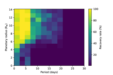
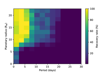
Figure 10: Injection-recovery tests performed on the TESS light curves of WASP-160A (left) and WASP-160B (right). Light and dark colors indicate high and low recovery rates, respectively. Planetary radii are corrected by the contamination due to the companion.

5 Planetary Analysis

5.1 Search for Additional Transiting Planets Around WASP-160A and WASP-160B from TESS Data

In order to constrain possible scenarios that could account for the chemical pattern observed in Figure 7, we searched for signs of additional transiting planets around both stars of the system using the TESS photometric data presented in Section 2.2.2. For the B component, we employed the light curve obtained in Section 2.2.2 but with the data-points of all the five transits of the planet removed. For the A star, we followed the same procedure applied for the secondary component to get the light curve. We picked up the pixel with the highest flux centered on the position of WASP-160A and performed single aperture photometry on it (Figure 2). As a consequence of the flux contamination by WASP-160B, this light curve showed some residual from the transits around the companion that we eliminated by removing the data-points at the times of all the transits. Lastly, we employed a Savitzky-Golay filter to smooth some remanent non-corrected systematics.

Once we obtained the detrended light curves of both components, we ran on each one separately the Transit Least Squares code (TLS, Hippke & Heller, 2019), an algorithm designed to search for periodic transits from time-series photometry. TLS did not detect any feature that could be clearly attributed to the transit of a new planet around any of the components.

Nonetheless, we performed two injection-recovery tests to evaluate the detection limits of transiting planets in the TESS light curves of both stars in the system. We explored the planetary radius-orbital period parameter-space, $R_{P}$-$P$, from 0.0 to 12.0 R_⊕ with a step of 1.0 R_⊕ for the planetary radius and from 0 to 30.0 days with a step of 2.5 days for the orbital period. The transit signals injected into the TESS light curves were generated with the BATMAN code (Kreidberg, 2015) assuming circular orbits and equatorial transits (inclination of 90 degrees). We considered a positive detection when the period recovered by the TLS code is within 5$\%$ of any half-multiple of the injected period. In Figure 10, we present the results of these tests. Planetary radii in the Y-axes are already corrected by a factor that accounts for the contamination due to the companion. In the case of the B component, this value was computed by EXOFASTv2 through the parameter FITDILUTE, whilst for the primary star we used the factor estimated for the companion and the dilution parameter “D”, as defined in Sullivan et al. (2015):

$${}D=\frac{F_{A}+F_{B}}{F_{A}}$$ (1)

where F_A and F_B are the fluxes of WASP-160A and WASP-160B, respectively, integrated in the TESS band.

The most important conclusion that arises from Figure 10 is that we might be able to detect, with high probability ($>$ 80$\%$), transiting planets larger than $\sim$ 5.5 R_⊕ and $\sim$ 7 R_⊕ with orbital periods shorter than $\sim$ 7 days around WASP-160A and WASP-160B, respectively. We do not expect a detection of planets at far distances from the stars (periods $>$ 20 days) or for small planets (radii $<$ 5.5 R_⊕) with orbital periods longer than $\sim$ 7 days in the case of WASP-160A, and small planets (radii $<$ 7 R_⊕) with orbital periods longer than $\sim$ 2.5 days for WASP-160B. The detection probabilities range from 20 to 80$\%$ for all the planets that occupied the parameter-space in between.

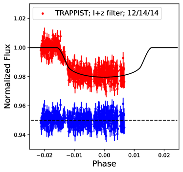
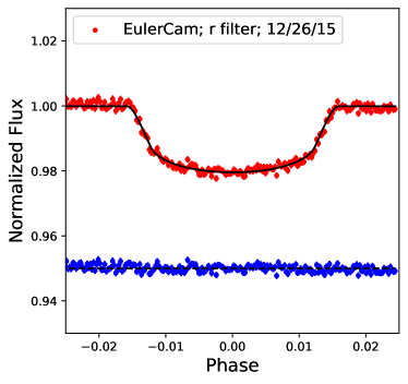
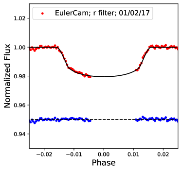
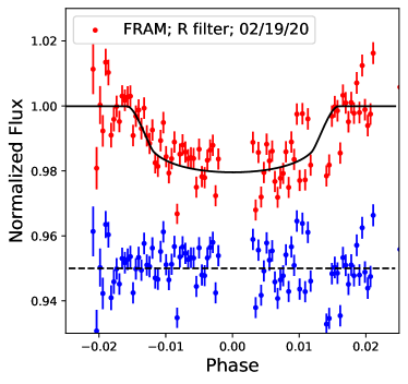
Figure 11: Ground-based light curves of WASP-160B. In the top part of each panel, the black solid line is the best-fit model from EXOFASTv2. The residual (data minus model) are shown at the bottom of each panel (in blue), where a horizontal dashed black line is plotted for reference. The observations are phase-folded to the period of the transiting planet. The names of the instruments and observation dates are denoted in boxes in the upper part of each panel.

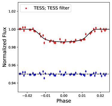
Figure 12: Phase folded TESS light curve (red) of WASP-160B. The black solid line is the best-fit model from EXOFASTv2. The residuals are plotted below (in blue), where a horizontal dashed black line is plotted for reference.

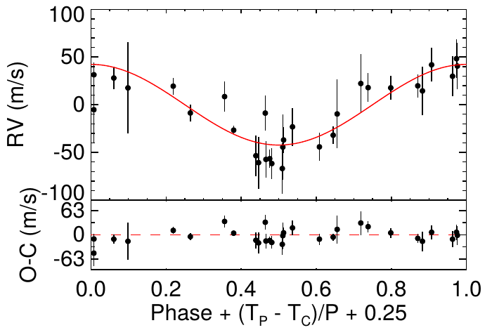
Figure 13: Radial velocity measurements of WASP-160B b from CORALIE phase folded to the best determined period from our global model. The red solid line is the best-fit model from EXOFASTv2. The residuals are plotted below. Here $T_{P}$ is the time of periastron, $T_{C}$ is the time of conjunction or transit, and $P$ is the orbital period.

5.2 Refined Planet Properties of WASP-160B b

We derived planetary and stellar properties of WASP-160B with the latest version of the EXOFASTv2 code (Eastman et al., 2013, 2019). We performed a simultaneous fit through a differential evolution Markov Chain Monte Carlo to the transit light curves and RV measurements presented in Section 2, the broadband photometry, Gaia DR2 parallax for WASP-160B and A_V extinction, and the effective temperature and metallicity derived in Section 3.1. All stellar properties are summarized in Table 2.

We set Gaussian priors for the parameters with independent constraints, namely T_eff, [Fe/H], parallax, and extinction, with widths corresponding to their one-sigma uncertainties. As for WASP-160A, we set an upper limit to the extinction of 0.04 to avoid unrealistic solutions based on the galactic dust maps by Schlafly & Finkbeiner (2011). Additionally, we used a Gaussian prior for the orbital period with its uncertainty derived by LE19, because we do not include the WASP light curve in this analysis which contributes significantly to the determination of the orbital period. We assumed a circular orbit. We used as starting points in M_⋆, R_⋆, and age, the values derived with q² presented in Section 3.3. Since these three parameters are not independent from the EXOFASTv2 analysis, we do not restrict them or set them as Gaussian priors in the fitting.

The physical properties of the planetary system are then derived by simultaneously fitting all the available data described above to a keplerian orbital motion, the transit model (Mandel & Agol, 2002), a single-star SED, and a set of stellar models, either MIST (Choi et al., 2016) or YY (Demarque et al., 2004). In the case of the TESS light curve, we accounted for the 30-min cadence of the observations by setting EXPTIME to 30 and NINTERP to 10, and for the dilution in the light curve due to WASP-160A, by fitting for the FITDILUTE parameter. Thus, we obtain two best-fit solutions for WASP-160B, one where the stellar properties are constrained with the MIST stellar models and a second one that is constrained with the YY stellar models. Each of the best-fit solutions are attained by starting the MCMC chains several times until all the data sets were optimally fitted. We ran EXOFASTv2 several times for each solution, using the same Gaussian priors, and after the first run, the starting points for the previous MIST or YY run, respectively. Each MCMC ran until the two convergence criteria were reached (number of independent draws T${}_{z}>$ 1000 and Gelman-Rubin statistic $<$ 1.01; as described in Eastman et al., 2013). As a check on our assumption that the planetary orbit is circular, we ran EXOFASTv2 allowing the eccentricity to be a free parameter using the same priors and the YY best-fit solution as a starting point. It resulted in a solution with a small eccentricity (0.03 ${}^{+0.03}_{-0.021}$), with a $\sim$97% probability of being spurious (see Lucy & Sweeney, 1971); thus confirming our choice for a circular orbit.

The derived physical properties for WASP-160B for the YY best-fit solution are presented in Table 2 for the host star, and in Table 5 of the Appendix A, for the transiting planet. We adopt the median values of the posterior distributions of each best-fit solution, and 68$\%$ confidence intervals as their one-sigma uncertainties. Both YY and MIST best-fit solutions are equivalent and consistent within their uncertainties. We have a slight preference for the best-fit solution derived from the YY models, because it allows us to compare our stellar properties with our other results minimizing systematic uncertainties arising from the choice of stellar models. Our refined planetary parameters are consistent within the errors with those found by LE19, but are more precise because of the refined stellar properties. In Figures 11 and 12, we show the resulting best-fit models for the ground-based and the TESS transit light curves, respectively, and in Figure 13 we show the best-fit model to the radial velocity measurements.

Additionally, we performed a linear fit to the mid-transit times computed with EXOFASTv2. Given that the resulting O-C values are all within 1$\sigma$ of a linear ephemeris, we do not find evidence of transit timing variations (TTVs) in the system. However, it is important to notice that the small number of transits analyzed in this work prevent us from fully discarding the existence of additional planets around WASP-160B with the TTVs analysis. Certainly, an intensive photometric follow-up to significantly increase the number of complete and high-quality transits available would place more robust constraints on the presence of intermediate-mass short-period planets in the system.

6 Discussion

6.1 Origin of the chemical differences

WASP-160A and B show a non-negligible difference in their chemical compositions (Figure 6) which also seems to correlate with the condensation temperature (Figure 7). In particular, we observe that WASP-160B is slightly depleted in volatiles ($-$0.035 dex, on average) and enhanced in refractory elements (+0.033 dex, on average) when compared to WASP-160A. To date, this kind of curious chemical pattern has been previously reported only in the binary system WASP-94 (Teske et al., 2016a), where each component hosts a hot Jupiter planet.

As discussed in Section 4, the $\Delta$[X/H]_B-A versus T_c correlation that we have detected cannot be only due to our particular choice of stellar parameters. The T_c trend is still present when we recomputed the abundances using: (i) spectroscopic fundamental parameters with solar reference, (ii) photometric T_eff and trigonometric $\log g$ values, and (iii) the fundamental parameters from LE19. Moreover, given the good agreement between our adopted $\Delta$T_eff value and those derived from independent techniques, it is unlikely that our computed temperatures could have produced the observed pattern. Also, we found no evidence that could link the observed abundance differences with their measured chromospheric activity. Under the reasonable and common assumption that the components of binary systems share their initial composition (e.g., Desidera et al., 2006; Andrews et al., 2019; Hawkins et al., 2020; Nelson et al., 2021), since they form coevally from the same molecular cloud, it is unlikely that their dissimilar abundances are caused by different Galactic chemical evolution (e.g., Adibekyan et al., 2014; Nissen, 2015) or different stellar environment effects (e.g., Önehag et al., 2014). Alternatively, as discussed in several previous studies of binary stars with similar components, the elemental abundance differences might be connected to processes of planetary formation and evolution (e.g., Ramírez et al., 2011, 2015; Teske et al., 2016a, b; Saffe et al., 2015, 2017; Oh et al., 2018; Nagar et al., 2020).

What is the origin of the differences in the abundance of volatile elements? It has been suggested that the formation of a giant planet with large volatile-rich envelopes would cause a decrease in the overall metallicity of its host star, and therefore also producing a depletion in the abundances of volatile elements (e.g., Ramírez et al., 2011, 2015; Tucci Maia et al., 2014; Teske et al., 2016a, b). Hence, the observed depletion of volatiles in WASP-160B, relative to WASP-160A, could be explained by the formation of the transiting giant planet, WASP-160B b, and/or other giant planets not yet detected in the system. As a first-order approximation, we can explore if the mass of WASP-160B b could account for the observed volatile differences using the corrected formula from Ramírez et al. (2011):

$${}\Delta[M/H]=\log\left[\frac{(Z/X)_{cz}M_{cz}+(Z/X)_{p}M_{p}}{(Z/X)_{cz}(M_{cz}+M_{p})}\right].$$ (2)

From the tracks by Siess et al. (2000), using the mass of WASP-160B, we estimated a present-day convective envelope mass $M_{cz}$ of 0.047 M_⊙. We adopt 0.1 for the planet metallicity $(Z/X)_{p}$ based on the solar system giant planets (e.g., Guillot, 2005; Fortney & Nettelmann, 2010; Ramírez et al., 2011), 0.28 M_J for the mass of WASP-160B b (see Table 5), and 0.019 for the stellar convection zone metallicity $(Z/X)_{cz}$ estimated by scaling the solar value of $(Z/X)_{\odot}$ of 0.0134 (Asplund et al., 2009) to the metallicity of WASP-160B ([Fe/H] = 0.151 dex). Interestingly, under these assumptions, the expected depletion in WASP-160B $\Delta[M/H]$ is $\sim$0.0104 dex, which is close to the observed difference in volatiles. Even a closer expected value of $\sim$0.025 dex can be obtained if the planet metallicity is slightly larger.

We note that the $M_{cz}$ that appears in Equation 2 corresponds to the convective zone at the time of planet formation, which for gas giants is suggested to occur on timescales shorter than $\sim$10 Myr (e.g., Pollack et al., 1996; Guilera et al., 2011). Alternative nonstandard models of stars with severe episodic accretion computed by Baraffe & Chabrier (2010) predict the $M_{cz}$ of a 1 M_⊙ star can reach its present-day thin size earlier than $\sim$10 Myr. Thus, as discussed in several previous studies (e.g., Chambers, 2010; Ramírez et al., 2011, 2014; Önehag et al., 2011; Melendez & Ramirez, 2016; Teske et al., 2016a; Nissen & Gustafsson, 2018; Spina et al., 2016, 2018; Tucci Maia et al., 2019), the hypothesis that planet formation (like WASP-160 B b) could have chemically altered the surface abundance pattern (i.e., depletion of volatiles) of its parent star would be plausible. However, as mentioned in Ramírez et al. (2014), the results from Baraffe & Chabrier (2010) also imply that the particular episodic accretion history of a star that forms planets will determine whether the chemical signature is imprinted or not. Moreover, recent stellar accreting models (Kunitomo et al., 2018) show that the evolution of the convective zone is relatively close to that of standard (non-accreting) pre-main-sequence evolutionary tracks for a $\sim$1 M_⊙ star.

Standard stellar models suggest that solar analog stars begin fully convective and reach their present-day low $M_{cz}$ only after $\sim$30 Myr (D’Antona & Mazzitelli, 1994; Murray et al., 2001; Serenelli et al., 2011). In this case, if instead we assume $M_{cz}$ = 0.4 M_⊙ for a $\sim$0.9 M_⊙ star at $\sim$10 Myr according to the standard model of Serenelli et al. (2011), the expected depletion in WASP-160B to explain the planet mass is only $\sim$0.002 dex, which is well below the observed offset in volatiles. If instead we assume a larger $M_{cz}$ of 0.7 M_⊙ (at $\sim$5 Myr), we expect a lower offset of 0.0008 dex.

Alternatively, we can reverse the Equation 2 and determine the mass of material that could explain the missing $\sim$0.035 dex of volatiles in WASP-160B. Considering the standard early convective envelopes of $M_{cz}$ = 0.4 M_⊙ and $M_{cz}$ = 0.7 M_⊙ for $(Z/X)_{p}$ = 0.1, we found that the mass required to explain the offset in volatiles is about 6 $M_{J}$ and 13 $M_{J}$, respectively. Therefore, in these cases, the formation of one or more gas-giant planets around WASP-160B, additional to the one already detected, would be needed to explain the observed depletion of volatiles.

The RV data from LE19 do not suggest the presence of additional giant planets in WASP-160B. However, we note that both the precision and time coverage of the CORALIE observations are not enough to fully reject the presence of a giant long period planet and/or additional lower mass bodies. As detailed in Section 5.1, we found no signs of additional transiting planets using the available TESS photometry, although we were only able to discard, with a probability higher than 80$\%$, the presence of large, close-in planets ($P$ $\lesssim$ 7 days) with $R_{P}$ $\gtrsim$ 7 R_⊕ (see Figure 10). However, as in the case of the RV data from LE19, the analyzed TESS photometric data is inconclusive with regards to the presence of smaller-size and/or longer-period planets. Furthermore, if additional bodies actually formed around WASP-160B, the non-detection of these planets might suggest that could have been ejected from the system by planet-planet interactions.

On the other hand, we need to combine the hypothesis above for the origin of the missing volatiles with possible scenarios to explain the enrichment of refractory elements in WASP-160B, relative to WASP-160A, and the weak upward T_c trend which is also observed in Figure 7. The chemical differences in refractories could be interpreted as the signature of either abundance depletion in WASP-160A or enhancement in WASP-160B:

-i) In the first case, the difference in refractory elements can be considered within the scenario proposed by M09 and Ramírez et al. (2011): the formation of rocky material (e.g., terrestrial planets, planetesimals) might result in a depletion of refractory elements (in comparison to volatiles) in the convective envelope of the host star, relative to its initial composition. Under this framework, we might interpret that refractory elements were sequestered from the protostellar nebula of WASP-160A to form rocky bodies while the volatiles were accreted onto the star. Using the model outlined in Chambers (2010), via the terra code (Yana Galarza et al., 2016), we find that $\sim$4.5 $M_{\oplus}$, where $M_{\oplus}$ is the mass of Earth, of material (with an Earth-like composition) are needed to explain the observed offset in the refractory elements which, as discussed in Sec. 4, also seem to show a weak correlation with T_c. As before, here we have assumed a present-day convection zone mass $M_{cz}$ = 0.039 M_⊙ for WASP-160A. If, as discussed before, instead we use larger convective envelopes at younger stellar ages such as $M_{cz}$ = 0.2 M_⊙ (at 15 Myr) and $M_{cz}$ = 0.4 $M_{\odot}$ (at 10 Myr), then $\sim$21 $M_{\oplus}$ and $\sim$47 $M_{\oplus}$ would be required to explain the observed trend .

To date, no planets have been reported to orbit WASP-160A. LE19 obtained eight CORALIE spectra of WASP-160A and found no evidence of any large-amplitude RV variability. In particular, they found that the RV measurements are stable within $\sim$40 ms^-1. Thus, it is unlikely that this star harbors a short-period giant planet similar to that found around WASP-160B. However, both the precision and time coverage of the RV data are not enough to fully reject the presence of a giant long period planet and/or a low mass body.

In an effort to investigate the existence of additional planets around WASP-160A which might account for the chemical pattern, as is detailed in Section 5.1, we searched for transiting planets using the available TESS photometry. We found no transit signals and we were able to discard, with a probability higher than 80$\%$, the presence of large, close-in planets ($P$ $\lesssim$ 7 days) with radii larger than 5.5 R_⊕ (see Figure 10). However, as in the case of the RV data from LE19, the analyzed TESS photometric data is inconclusive with regards to the presence of small and/or longer-period planets ($P$ $\geq$ 20 days). Long-term RV follow-up and/or additional photometric monitoring of WASP-160A might help to constrain the possible formation of planets around this star. For example, the TESS extended mission will observe WASP-160 in sectors 32 and 33 broadening the search to planets with periods within a few tens of days and increasing the chance of monotransit detections (e.g., Cooke et al., 2019). Future space telescopes within the next decade will also extend the search for planets, with observations of reflected light with Roman Space Telescope (e.g., Carrión-González et al., 2020), and to smaller planets and long periods, if WASP-160 is within the selected fields of PLATO (Rauer et al., 2014).

We also tried to provide initial restrictions on the formation of planetesimals or/and asteroids around WASP-160A by investigating the presence of circumstellar material around this star. Saffe et al. (2016) proposed that the refractory-elements depleted in $\zeta^{2}$ Ret, relative to its twin binary companion $\zeta^{1}$ Ret, are locked-up in the rocky material that produce the debris disk observed around this object (although see Faramaz et al., 2018). Since the computed missing mass of refractories in WASP-160A is roughly compatible with the masses estimated for debris disks around solar-type stars (3-50 M_⊕; Krivov et al., 2008), we could consider a similar scenario to explain the lack of refractories in WASP-160A. Nevertheless, we find no signs of infrared excess on the SEDs, obtained in Sections 3.2 and 3.3, that could be associated with circumstellar dust around WASP-160A. We caution, however, that the magnitudes employed to obtain the SEDs are restricted to mid-IR bands only and therefore the analysis is inconclusive with regards to the presence of cold debris disks at large radial distances. Additional observations in the far-IR and (sub-)millimeter wavelength regions and/or high-contrast imaging combined with high-precision polarimetry, would provide better constraints on the formation of planetesimals around WASP-160A.

-ii) In the second scenario, after the initial decrease in the overall metallicity and volatile abundances in WASP-160B, allegedly caused by the formation of the Saturn-mass planet and possibly additional ones, late-time accretion of refractory-rich planetary material onto WASP-160B could have enhanced the abundance of high-T_c elements producing the observed trend. The rocky bodies could have been pushed or dragged onto WASP-160B during the inward migration of the gas giant planet (e.g., Pinsonneault et al., 2001; Ford & Rasio, 2008; Sandquist et al., 2002; Ida & Lin, 2008; Raymond et al., 2011; Mustill et al., 2015) or by perturbations caused by its wide stellar companion (e.g., Kaib et al., 2013). Again, using terra we can estimate the amount of refractory-rich material accreted by WASP-160B for different convective envelopes sizes to reproduce the observed T_c trend. For the present-day convective envelope of 0.047 M_⊙, we find that $\sim$6 M_⊕ of material (with an Earth-like composition) are needed to explain the observed T_c trend in the refractory elements. This value rises up to $\sim$24 $M_{\oplus}$ if we consider $M_{cz}$ = 0.2 $M_{\odot}$ (at 15 Myr) and up to $\sim$48 M_⊕ for $M_{cz}$ = 0.4 M_⊙ (at 10 Myr). We caution that this result does not necessarily imply that WASP-160A did not engulf rocky material also, but instead would suggest that WASP-160B accreted a larger amount of material than the primary.

As suggested in the case of other binary systems (e.g., Saffe et al., 2017; Oh et al., 2018), it would be expected that the accretion of planetary material on the atmosphere of WASP-160B would also produce an enhancement in its abundance of lithium, relative to that of WASP-160A. Nevertheless, as we mention in Sec. 3.4, for both stars in WASP-160 we only could derive an upper limit of their abundances (A(Li) $\lesssim$ 0.17 dex and A(Li) $\lesssim$ 0.6 dex for WASP-160A and B, respectively), which are normal for their old ages and T_eff values (Ramírez et al., 2011; Aguilera-Gómez et al., 2018). Although these results might not support a pollution scenario, we should stress that the behavior of Li abundances in solar-type stars with planets is very complex, not yet fully understood, and still debated (e.g., Chaboyer, 1998; Israelian et al., 2009; Pinsonneault, 2010; Ghezzi et al., 2010; Baumann et al., 2010; Ramírez et al., 2012; Figueira et al., 2014; Delgado Mena et al., 2015; Mishenina et al., 2016). Moreover, as discussed in Meléndez et al. (2017), it is difficult to quantify the net amount of Li enhancement because it depends on several factors such as the initial stellar lithium content at the time of accretion, the time of accretion, Li depletion since the planet accretion, and the real effect and efficiency of thermohaline mixing for the depletion of Li (e.g., Théado & Vauclair, 2012).

Finally, Booth & Owen (2020) recently proposed an alternative hypothesis to that of M09. According to this new scenario, the depletion of refractories in the Sun does not arise from the sequestration of refractory material inside the planets themselves but instead from the gap, and pressure trap, created by the formation of a Jupiter analog planet that prevents the accretion of the dust (refractories) exterior to its orbit onto the star in contrast to the gas (volatiles). For the case of WASP-160, however, it is not clear how this mechanism would explain the chemical pattern observed in Figure 7. If we consider only the planet orbiting WASP-160B, according to the hypothesis of Booth & Owen (2020) this star should show low abundances of refractories relative to volatiles but we observe the opposite trend. On the other hand, if also a Jupiter analog formed around WASP-160A, in order to explain the chemical trend, the pressure trap created by this planet should have been more effective in impeding the accretion of refractory material onto the host star than the confirmed Saturn-mass planet around WASP-160B. Although the latter could perhaps be related by the migration history of WASP-160B b or its mass, the observed dissimilar composition of volatiles is hard to reconcile since in this framework the abundances of these elements should not be affected by the gaps. A detailed simulation within the scenario of Booth & Owen (2020) for WASP-160, which is beyond the scope of this paper, might provide additional constraints on how this mechanism could explain the observed chemical pattern for this binary system.

6.2 Abundance differences and binary separation

Ramírez et al. (2019, hereafter RA19) studied a sample of twelve binary systems (with and without planets) with available high-precision chemical abundances in the literature to search for correlations with stellar parameters and/or binary star characteristics. They found a weak correlation between the absolute value of elemental abundance differences and binary star projected separation. In particular, the differences seem to increase as the distance between the stars in each pair becomes larger. Moreover, the differences become more significant for species that are least abundant in the Sun’s photosphere (e.g., Sr, Zr, Rb, Y, Ba) compared to those species that are more abundant (e.g., O, C; see their Fig. 9). RA19 proposed that this could be an effect produced by the chemical inhomogeneity of the gas clouds from which the binary stars formed. Furthermore, RA19 emphasized that their results do not compromise the significance of the T_c trends previously found on binary systems and/or their interpretation as due to sequestering or ingestion of planetary material. Instead, the authors suggest that the effect of chemical inhomogeneity might blur the T_c trends observed in some binaries.

Using our computed abundances and the projected separation between the components of WASP-160, we checked if this system could also follow the weak correlation presented by RA19. We found that the WASP-160 data is consistent with the trend for elements with high solar absolute abundance (O, C), in which there is a small system-to-system $\Delta$[X/H] variation. The elements with a lower absolute abundance in the Sun tend to show larger relative differences, in comparison to the results obtained with O and C. Nevertheless, they are not as large as would be expected for a system with the projected separation of WASP-160. Overall, under the scenario proposed by RA19, the results for WASP-160 might suggest that the molecular cloud from which this pair formed was more chemical homogeneous relative to other analyzed systems. However, since the correlations presented by RA19 are of second order, an analysis with a larger sample of binary systems will allow us to better understand the results for WASP-160.

7 Summary and Conclusions

In this work, we have expanded the small sample of well-studied planet-hosting binary stars by performing a detailed characterization of the WASP-160 stellar pair. No planet has yet been reported around WASP-160A while WASP-160B hosts a short-period transiting Saturn-mass planet, WASP-160B b. For this planet, we also derived refined properties by performing a global fit that includes our precise stellar parameters, literature data, and new observations. Furthermore, based on TESS photometry, we constrained the presence of transiting planets around WASP-160A and additional ones around WASP-160B. Our injection-recovery analysis allowed us to discard, with high probability ($>$ 80$\%$), the presence of transiting planets with orbital periods $\lesssim$ 7 days, and radii $>$ 5.5 $R_{\mathrm{\oplus}}$ and $>$ 7 $R_{\mathrm{\oplus}}$ around WASP-160A and WASP-160B, respectively.

The stellar characterization included, for the first time, the computation of high-precision and strictly differential atmospheric parameters and chemical abundances of 25 elements based on high-quality spectra. The analysis revealed that WASP-160B is slightly but significantly depleted in volatiles and enhanced in refractory elements relative to WASP-160A. Therefore we found evidence of a nonzero slope trend between $\Delta$[X/H] and T_c. Interestingly, this curious chemical pattern showing both depletion of volatiles and enhancement of refractories has been previously reported only in the binary system WASP-94, where each star hosts a hot Jupiter planet (Teske et al., 2016a).

We discussed that the depletion of volatiles could be explained by the formation of the observed Saturn-mass planet WASP-160B b if we assume the present-day $M_{cz}$ of the host star, but single or multiple additional planets (to add up to $\sim$6$-$13 $M_{J}$) are required when adopting a larger $M_{cz}$. On the other hand, the refractory-difference could be explained by (i) the formation of rocky bodies (at least $\sim$4.5 $M_{\oplus}$) around WASP-160A or (ii) the late accretion of at least $\sim$6 $M_{\oplus}$ of planet-like material by WASP-160B.

The formation of the confirmed short-period giant planet orbiting WASP-160B and later accretion of planet-like material by this star, likely triggered by the inward migration of the giant planet, represents a tantalizing scenario to explain the observed anomalous chemical pattern. However, the detection limits provided by the current photometric and RV data along with the significant dependence on the assumed $M_{cz}$ prevent us from fully supporting this last hypothesis over the formation of additional (long period) giant planets in WASP-160B and those of the rocky kind around WASP-160A. Future long-term high-precision photometric and RV follow-up, as well as high-contrast imaging observations, of WASP-160A and B, would provide further constraints and might reveal the real origin of the peculiar chemical differences observed.

Appendix A Additional tables

Table 3: Adopted Atomic Data and Measured Equivalent Widths

Wavelength	Species	EP	$\log gf$	WASP-160A	WASP-160B	Sun
(Å)		(eV)		(mÅ)	(mÅ)	EW (mÅ)
6587.61	6.0	8.537	$-$1.021	10.0	6.3	14.3
5380.34	6.0	7.685	$-$1.570	14.4	9.7	20.8
9078.28	6.0	7.480	$-$0.581	73.5	53.7	110.0
9111.80	6.0	7.490	$-$0.297	97.5	74.0	140.0
7468.27	7.0	10.340	$-$0.150	7.8	5.0	4.6
8683.40	7.0	10.330	$-$0.050	10.0	6.3	8.0
7775.39	8.0	9.146	0.002	33.5	24.2	44.5
7774.16	8.0	9.150	0.220	43.0	31.5	58.7
7771.94	8.0	9.146	0.352	49.5	33.5	69.2

Table 4: Condensation Temperatures, Number of Measured lines, and Elemental Abundances Relative to Solar ([X/H]) and Differential Between WASP-160A and WASP-160B ($\Delta$[X/H]_B-A)

Species	Tc (K)	Nlines	[X/H] (dex)	Error (dex)	[X/H] (dex)	Error (dex)	$\Delta$[X/H]B-A (dex)	Error (dex)
			(WASP-160A)		(WASP-160B)
C i	40	4	$-$0.021	0.094	$-$0.097	0.090	$-$0.049	0.005
N i	131	2	0.560	0.064	0.538	0.068	$-$0.022	0.007
O i	180	3	0.130	0.021	0.118	0.052	$-$0.010	0.023
Na i	958	4	0.312	0.026	0.321	0.029	0.008	0.005
Mg i	1336	3	0.141	0.079	0.172	0.073	0.031	0.006
Al i	1653	3	0.263	0.059	0.294	0.060	0.031	0.007
Si i	1310	28	0.165	0.062	0.181	0.074	0.015	0.007
S i	664	3	0.259	0.137	0.243	0.154	$-$0.010	0.012
K i	1006	1	$-$0.152	0.172	$-$0.200	0.167	$-$0.048	0.028
Ca i	1517	8	0.161	0.051	0.170	0.052	0.017	0.008
Sc i	1659	3	0.189	0.099	0.254	0.121	0.065	0.029
Sc ii	1659	7	0.215	0.048	0.265	0.046	0.050	0.007
Ti i	1582	18	0.197	0.055	0.252	0.054	0.055	0.006
Ti ii	1582	2	0.150	0.004	0.222	0.012	0.069	0.010
V i	1429	6	0.262	0.081	0.381	0.082	0.099	0.017
Cr i	1296	10	0.149	0.057	0.202	0.058	0.053	0.006
Cr ii	1296	3	0.149	0.012	0.211	0.006	0.067	0.012
Mn i	1158	3	0.163	0.102	0.206	0.166	0.043	0.008
Fe i	1334	84	0.137	0.051	0.145	0.052	0.008	0.005
Fe ii	1334	10	0.151	0.079	0.164	0.080	0.012	0.007
Co i	1352	5	0.161	0.065	0.171	0.057	0.070	0.007
Ni i	1353	40	0.183	0.067	0.205	0.064	0.022	0.005
Cu i	1037	3	0.353	0.179	0.410	0.205	0.056	0.019
Zn i	726	1	$-$0.039	0.172	$-$0.075	0.166	$-$0.036	0.026
Rb i	800	2	$-$0.391	0.172	$-$0.383	0.141	0.008	0.031
Y ii	1659	2	0.163	0.024	0.223	0.032	0.060	0.010
Zr ii	1741	1	0.041	0.172	0.067	0.166	0.026	0.028
Ba ii	1455	2	0.063	0.047	0.102	0.032	0.039	0.018
Eu ii	1356	1	0.305	0.172	0.388	0.166	0.083	0.026

Table 5: Median values and 68% confidence interval for the Physical and Orbital Parameters of WASP-160B b

Parameter	Units	Values YY (circular)	Values MIST (circular)
$P$	Period (days)	$3.7684935\pm 0.0000016$	$3.7684935^{+0.0000016}_{-0.0000015}$
$a$	Semi-major axis (AU)	$0.04541^{+0.00037}_{-0.00035}$	$0.04536^{+0.00067}_{-0.00056}$
$R_{P}$	Radius ($R_{\mathrm{J}}$)	$1.093^{+0.022}_{-0.021}$	$1.093^{+0.023}_{-0.022}$
$M_{P}$	Mass ($M_{\mathrm{J}}$)	$0.281\pm 0.030$	$0.280\pm 0.031$
$\rho_{P}$	Density (cgs)	$0.266^{+0.033}_{-0.032}$	$0.266^{+0.033}_{-0.032}$
$logg_{P}$	Surface gravity (cgs)	$2.765^{+0.048}_{-0.052}$	$2.764^{+0.048}_{-0.052}$
$T_{eq}$	Equilibrium temperature (K)	$1099.5^{+9.0}_{-8.9}$	$1099.5^{+9.0}_{-8.9}$
$\Theta$	Safronov Number	$0.0265\pm 0.0029$	$0.0264\pm 0.0029$
$\langle F\rangle$	Incident Flux (109 erg s-1 cm-2)	$0.331^{+0.011}_{-0.010}$	$0.331\pm 0.011$
Primary transit parameters:
$R_{P}/R_{*}$	Radius of planet in stellar radii	$0.12877^{+0.00093}_{-0.00095}$	$0.12878^{+0.00093}_{-0.00094}$
$a/R_{*}$	Semi-major axis in stellar radii	$11.2^{+0.19}_{-0.18}$	$11.19^{+0.19}_{-0.18}$
$i$	Inclination (Degrees)	$88.80^{+0.49}_{-0.33}$	$88.79^{+0.49}_{-0.33}$
$b$	Transit Impact parameter	$0.234^{+0.061}_{-0.093}$	$0.235^{+0.061}_{-0.094}$
$\delta$	Transit depth (fraction)	$0.01658\pm 0.00024$	$0.01658\pm 0.00024$
$T_{FWHM}$	FWHM transit duration (days)	$0.10425^{+0.00047}_{-0.00046}$	$0.10424\pm 0.00046$
$\tau$	Ingress/egress transit duration (days)	$0.01426^{+0.00057}_{-0.00058}$	$0.01426^{+0.00058}_{-0.00059}$
$T_{14}$	Total transit duration (days)	$0.11852^{+0.00057}_{-0.00056}$	$0.11851^{+0.00057}_{-0.00056}$
$P_{T}$	A priori non-grazing transit prob	$0.0778\pm 0.0012$	$0.0778\pm 0.0012$
$P_{T,G}$	A priori transit prob	$0.1008\pm 0.0017$	$0.1008\pm 0.0017$
$d/R_{*}$	Separation at mid transit	$11.20^{+0.19}_{-0.18}$	$11.19^{+0.19}_{-0.18}$
$Depth$	Flux decrement at mid transit	$0.01658\pm 0.00024$	$0.01658\pm 0.00024$
$u_{1R}$	linear limb-darkening coeff	$0.485^{+0.048}_{-0.049}$	$0.485\pm 0.048$
$u_{1r’}$	linear limb-darkening coeff	$0.503\pm 0.025$	$0.504\pm 0.025$
$u_{1z’}$	linear limb-darkening coeff	$0.304^{+0.040}_{-0.041}$	$0.303\pm 0.041$
$u_{1TESS}$	linear limb-darkening coeff	$0.400\pm 0.046$	$0.401\pm 0.046$
$u_{2R}$	quadratic limb-darkening coeff	$0.199\pm 0.049$	$0.198^{+0.050}_{-0.049}$
$u_{2r’}$	quadratic limb-darkening coeff	$0.189\pm 0.033$	$0.189\pm 0.033$
$u_{2z’}$	quadratic limb-darkening coeff	$0.231\pm 0.047$	$0.231\pm 0.047$
$u_{2TESS}$	quadratic limb-darkening coeff	$0.222\pm 0.049$	$0.221\pm 0.048$
$A_{D}$ (TESS)	Dilution from neighboring stars	$0.281\pm 0.019$	$0.281\pm 0.019$
Radial velocity parameters:
$T_{C}$	Time of conjunction (BJDTDB)	$2457383.65491\pm 0.00012$	$2457383.65491\pm 0.00012$
$T_{0}$	Optimal conjunction Time (BJDTDB)	$2457504.24670\pm 0.00011$	$2457504.24670^{+0.00011}_{-0.00010}$
$T_{P}$	Time of Periastron (BJDTDB)	$2457383.65491\pm 0.00012$	$2457383.65491\pm 0.00012$
$T_{S}$	Time of eclipse (BJDTDB)	$2457385.53915\pm 0.00012$	$2457385.53915\pm 0.00012$
$T_{A}$	Time of Ascending Node (BJDTDB)	$2457386.48128\pm 0.00012$	$2457386.48128\pm 0.00012$
$T_{D}$	Time of Descending Node (BJDTDB)	$2457384.59703\pm 0.00012$	$2457384.59703\pm 0.00012$
$K$	RV semi-amplitude (m s-1)	$39.9^{+4.2}_{-4.3}$	$39.8^{+4.2}_{-4.3}$
$M_{P}\sin i$	Minimum mass (Mp)	$0.281\pm 0.030$	$0.280\pm 0.031$
$M_{P}/M_{*}$	Mass ratio	$0.000305\pm 0.000033$	$0.000304\pm 0.000033$
$\gamma_{\rm CORALIE}$	Relative RV Offset (m s-1)	$-6141.7^{+3.2}_{-3.3}$	$-6141.7^{+3.2}_{-3.3}$

References

- Adibekyan et al. (2014) Adibekyan, V. Z., González Hernández, J. I., Delgado Mena, E., et al. 2014, A&A, 564, L15, doi: 10.1051/0004-6361/201423435
- Aguilera-Gómez et al. (2018) Aguilera-Gómez, C., Ramírez, I., & Chanamé, J. 2018, A&A, 614, A55, doi: 10.1051/0004-6361/201732209
- Aller et al. (2020) Aller, A., Lillo-Box, J., Jones, D., Miranda, L. F., & Barceló Forteza, S. 2020, A&A, 635, A128, doi: 10.1051/0004-6361/201937118
- Alves et al. (2019) Alves, F. O., Caselli, P., Girart, J. M., et al. 2019, Science, 366, 90, doi: 10.1126/science.aaw3491
- Amarsi et al. (2019) Amarsi, A. M., Nissen, P. E., & Skúladóttir, Á. 2019, A&A, 630, A104, doi: 10.1051/0004-6361/201936265
- Andrews et al. (2019) Andrews, J. J., Anguiano, B., Chanamé, J., et al. 2019, ApJ, 871, 42, doi: 10.3847/1538-4357/aaf502
- Andrews et al. (2017) Andrews, J. J., Chanamé, J., & Agüeros, M. A. 2017, MNRAS, 472, 675, doi: 10.1093/mnras/stx2000
- Asplund et al. (2009) Asplund, M., Grevesse, N., Sauval, A. J., & Scott, P. 2009, ARA&A, 47, 481, doi: 10.1146/annurev.astro.46.060407.145222
- Astropy Collaboration et al. (2018) Astropy Collaboration, Price-Whelan, A. M., Sipőcz, B. M., et al. 2018, AJ, 156, 123, doi: 10.3847/1538-3881/aabc4f
- Baraffe & Chabrier (2010) Baraffe, I., & Chabrier, G. 2010, A&A, 521, A44, doi: 10.1051/0004-6361/201014979
- Baumann et al. (2010) Baumann, P., Ramírez, I., Meléndez, J., Asplund, M., & Lind, K. 2010, A&A, 519, A87, doi: 10.1051/0004-6361/201015137
- Bayo et al. (2008) Bayo, A., Rodrigo, C., Barrado Y Navascués, D., et al. 2008, A&A, 492, 277, doi: 10.1051/0004-6361:200810395
- Bedell et al. (2014) Bedell, M., Meléndez, J., Bean, J. L., et al. 2014, ApJ, 795, 23, doi: 10.1088/0004-637X/795/1/23
- Bedell et al. (2017) Bedell, M., Bean, J. L., Meléndez, J., et al. 2017, ApJ, 839, 94, doi: 10.3847/1538-4357/aa6a1d
- Bedell et al. (2018) —. 2018, ApJ, 865, 68, doi: 10.3847/1538-4357/aad908
- Bensby et al. (2014) Bensby, T., Feltzing, S., & Oey, M. S. 2014, A&A, 562, A71, doi: 10.1051/0004-6361/201322631
- Bernkopf et al. (2001) Bernkopf, J., Fidler, A., & Fuhrmann, K. 2001, in Astronomical Society of the Pacific Conference Series, Vol. 245, Astrophysical Ages and Times Scales, ed. T. von Hippel, C. Simpson, & N. Manset, 207
- Biazzo et al. (2015) Biazzo, K., Gratton, R., Desidera, S., et al. 2015, A&A, 583, A135, doi: 10.1051/0004-6361/201526375
- Booth & Owen (2020) Booth, R. A., & Owen, J. E. 2020, MNRAS, 493, 5079, doi: 10.1093/mnras/staa578
- Bressan et al. (2012) Bressan, A., Marigo, P., Girardi, L., et al. 2012, MNRAS, 427, 127, doi: 10.1111/j.1365-2966.2012.21948.x
- Busà et al. (2007) Busà, I., Aznar Cuadrado, R., Terranegra, L., Andretta, V., & Gomez, M. T. 2007, A&A, 466, 1089, doi: 10.1051/0004-6361:20065588
- Carrión-González et al. (2020) Carrión-González, Ó., García Muñoz, A., Cabrera, J., et al. 2020, A&A, 640, A136, doi: 10.1051/0004-6361/202038101
- Casagrande et al. (2010) Casagrande, L., Ramírez, I., Meléndez, J., Bessell, M., & Asplund, M. 2010, A&A, 512, A54, doi: 10.1051/0004-6361/200913204
- Castelli & Kurucz (2003) Castelli, F., & Kurucz, R. L. 2003, in IAU Symposium, Vol. 210, Modelling of Stellar Atmospheres, ed. N. Piskunov, W. W. Weiss, & D. F. Gray, A20
- Chaboyer (1998) Chaboyer, B. 1998, in New Eyes to See Inside the Sun and Stars, ed. F.-L. Deubner, J. Christensen-Dalsgaard, & D. Kurtz, Vol. 185, 25. https://arxiv.org/abs/astro-ph/9803106
- Chambers (2010) Chambers, J. E. 2010, ApJ, 724, 92, doi: 10.1088/0004-637X/724/1/92
- Chene et al. (2014) Chene, A.-N., Padzer, J., Barrick, G., et al. 2014, in Society of Photo-Optical Instrumentation Engineers (SPIE) Conference Series, Vol. 9151, Society of Photo-Optical Instrumentation Engineers (SPIE) Conference Series, 47, doi: 10.1117/12.2057417
- Choi et al. (2016) Choi, J., Dotter, A., Conroy, C., et al. 2016, ApJ, 823, 102, doi: 10.3847/0004-637X/823/2/102
- Cooke et al. (2019) Cooke, B. F., Pollacco, D., & Bayliss, D. 2019, A&A, 631, A83, doi: 10.1051/0004-6361/201936703
- D’Antona & Mazzitelli (1994) D’Antona, F., & Mazzitelli, I. 1994, ApJS, 90, 467, doi: 10.1086/191867
- Delgado Mena et al. (2015) Delgado Mena, E., Bertrán de Lis, S., Adibekyan, V. Z., et al. 2015, A&A, 576, A69, doi: 10.1051/0004-6361/201425433
- Demarque et al. (2004) Demarque, P., Woo, J.-H., Kim, Y.-C., & Yi, S. K. 2004, The Astrophysical Journal Supplement Series, 155, 667, doi: 10.1086/424966
- Desidera et al. (2006) Desidera, S., Gratton, R. G., Lucatello, S., & Claudi, R. U. 2006, A&A, 454, 581, doi: 10.1051/0004-6361:20064896
- Eastman et al. (2013) Eastman, J., Gaudi, B. S., & Agol, E. 2013, PASP, 125, 83, doi: 10.1086/669497
- Eastman et al. (2019) Eastman, J. D., Rodriguez, J. E., Agol, E., et al. 2019, arXiv e-prints, arXiv:1907.09480. https://arxiv.org/abs/1907.09480
- Ecuvillon et al. (2004) Ecuvillon, A., Israelian, G., Santos, N. C., et al. 2004, A&A, 418, 703, doi: 10.1051/0004-6361:20035717
- Egeland et al. (2017) Egeland, R., Soon, W., Baliunas, S., et al. 2017, ApJ, 835, 25, doi: 10.3847/1538-4357/835/1/25
- Epstein et al. (2010) Epstein, C. R., Johnson, J. A., Dong, S., et al. 2010, ApJ, 709, 447, doi: 10.1088/0004-637X/709/1/447
- Faramaz et al. (2018) Faramaz, V., Bryden, G., Stapelfeldt, K. R., et al. 2018, MNRAS, 481, 44, doi: 10.1093/mnras/sty2304
- Figueira et al. (2014) Figueira, P., Faria, J. P., Delgado-Mena, E., et al. 2014, A&A, 570, A21, doi: 10.1051/0004-6361/201424218
- Ford & Rasio (2008) Ford, E. B., & Rasio, F. A. 2008, ApJ, 686, 621, doi: 10.1086/590926
- Fortney & Nettelmann (2010) Fortney, J. J., & Nettelmann, N. 2010, Space Sci. Rev., 152, 423, doi: 10.1007/s11214-009-9582-x
- Gaia Collaboration et al. (2018) Gaia Collaboration, Brown, A. G. A., Vallenari, A., et al. 2018, A&A, 616, A1, doi: 10.1051/0004-6361/201833051
- Gaidos (2015) Gaidos, E. 2015, ApJ, 804, 40, doi: 10.1088/0004-637X/804/1/40
- Ghezzi et al. (2010) Ghezzi, L., Cunha, K., Smith, V. V., & de la Reza, R. 2010, ApJ, 724, 154, doi: 10.1088/0004-637X/724/1/154
- Gonzalez (1997) Gonzalez, G. 1997, MNRAS, 285, 403, doi: 10.1093/mnras/285.2.403
- Guilera et al. (2011) Guilera, O. M., Fortier, A., Brunini, A., & Benvenuto, O. G. 2011, A&A, 532, A142, doi: 10.1051/0004-6361/201015731
- Guillot (2005) Guillot, T. 2005, Annual Review of Earth and Planetary Sciences, 33, 493, doi: 10.1146/annurev.earth.32.101802.120325
- Hawkins et al. (2020) Hawkins, K., Lucey, M., Ting, Y.-S., et al. 2020, MNRAS, 492, 1164, doi: 10.1093/mnras/stz3132
- Hellier et al. (2011) Hellier, C., Anderson, D. R., Collier Cameron, A., et al. 2011, in European Physical Journal Web of Conferences, Vol. 11, European Physical Journal Web of Conferences, 01004, doi: 10.1051/epjconf/20101101004
- Henry et al. (1996) Henry, T. J., Soderblom, D. R., Donahue, R. A., & Baliunas, S. L. 1996, AJ, 111, doi: 10.1086/117796
- Hinkel et al. (2016) Hinkel, N. R., Young, P. A., Pagano, M. D., et al. 2016, ApJS, 226, 4, doi: 10.3847/0067-0049/226/1/4
- Hippke & Heller (2019) Hippke, M., & Heller, R. 2019, A&A, 623, A39, doi: 10.1051/0004-6361/201834672
- Ida & Lin (2008) Ida, S., & Lin, D. N. C. 2008, ApJ, 673, 487, doi: 10.1086/523754
- Israelian et al. (2009) Israelian, G., Delgado Mena, E., Santos, N. C., et al. 2009, Nature, 462, 189, doi: 10.1038/nature08483
- Janeček et al. (2019) Janeček, P., Ebr, J., Juryšek, J., et al. 2019, in European Physical Journal Web of Conferences, Vol. 197, European Physical Journal Web of Conferences, 02008, doi: 10.1051/epjconf/201919702008
- Jofré et al. (2015) Jofré, E., Petrucci, R., Saffe, C., et al. 2015, A&A, 574, A50, doi: 10.1051/0004-6361/201424474
- Jofré et al. (2020) Jofré, E., Almenara, J. M., Petrucci, R., et al. 2020, A&A, 634, A29, doi: 10.1051/0004-6361/201936446
- Jofré et al. (2017) Jofré, P., Heiter, U., Worley, C. C., et al. 2017, A&A, 601, A38, doi: 10.1051/0004-6361/201629833
- Kaib et al. (2013) Kaib, N. A., Raymond, S. N., & Duncan, M. 2013, Nature, 493, 381, doi: 10.1038/nature11780
- Kass & Raftery (1995) Kass, R. E., & Raftery, A. E. 1995, J. Am. Stat. Assoc., 90, 773, doi: 10.1080/01621459.1995.10476572
- Kilic et al. (2017) Kilic, M., Munn, J. A., Harris, H. C., et al. 2017, ApJ, 837, 162, doi: 10.3847/1538-4357/aa62a5
- King et al. (2012) King, R. R., Parker, R. J., Patience, J., & Goodwin, S. P. 2012, MNRAS, 421, 2025, doi: 10.1111/j.1365-2966.2012.20437.x
- Kratter (2011) Kratter, K. M. 2011, in Astronomical Society of the Pacific Conference Series, Vol. 447, Evolution of Compact Binaries, ed. L. Schmidtobreick, M. R. Schreiber, & C. Tappert, 47. https://arxiv.org/abs/1109.3740
- Kreidberg (2015) Kreidberg, L. 2015, PASP, 127, 1161, doi: 10.1086/683602
- Krivov et al. (2008) Krivov, A. V., Müller, S., Löhne, T., & Mutschke, H. 2008, ApJ, 687, 608, doi: 10.1086/591507
- Kunitomo et al. (2018) Kunitomo, M., Guillot, T., Ida, S., & Takeuchi, T. 2018, A&A, 618, A132, doi: 10.1051/0004-6361/201833127
- Lendl et al. (2019) Lendl, M., Anderson, D. R., Bonfanti, A., et al. 2019, MNRAS, 482, 301, doi: 10.1093/mnras/sty2667
- Lightkurve Collaboration et al. (2018) Lightkurve Collaboration, Cardoso, J. V. d. M., Hedges, C., et al. 2018, Lightkurve: Kepler and TESS time series analysis in Python, Astrophysics Source Code Library. http://ascl.net/1812.013
- Liu et al. (2020) Liu, F., Yong, D., Asplund, M., et al. 2020, MNRAS, 495, 3961, doi: 10.1093/mnras/staa1420
- Liu et al. (2014) Liu, Y. J., Tan, K. F., Wang, L., et al. 2014, ApJ, 785, 94, doi: 10.1088/0004-637X/785/2/94
- Lodders (2003) Lodders, K. 2003, ApJ, 591, 1220, doi: 10.1086/375492
- Lorenzo-Oliveira et al. (2016) Lorenzo-Oliveira, D., Porto de Mello, G. F., Dutra-Ferreira, L., & Ribas, I. 2016, A&A, 595, A11, doi: 10.1051/0004-6361/201628825
- Lucy & Sweeney (1971) Lucy, L. B., & Sweeney, M. A. 1971, AJ, 76, 544, doi: 10.1086/111159
- Mack et al. (2014) Mack, Claude E., I., Schuler, S. C., Stassun, K. G., & Norris, J. 2014, ApJ, 787, 98, doi: 10.1088/0004-637X/787/2/98
- Maldonado & Villaver (2016) Maldonado, J., & Villaver, E. 2016, A&A, 588, A98, doi: 10.1051/0004-6361/201527883
- Mandel & Agol (2002) Mandel, K., & Agol, E. 2002, ApJ, 580, L171, doi: 10.1086/345520
- Martin et al. (2017) Martin, J., Fuhrmeister, B., Mittag, M., et al. 2017, arXiv e-prints, arXiv:1708.04895. https://arxiv.org/abs/1708.04895
- Martioli et al. (2012) Martioli, E., Teeple, D., Manset, N., et al. 2012, in Society of Photo-Optical Instrumentation Engineers (SPIE) Conference Series, Vol. 8451, 2, doi: 10.1117/12.926627
- Meléndez et al. (2009) Meléndez, J., Asplund, M., Gustafsson, B., & Yong, D. 2009, ApJ, 704, L66, doi: 10.1088/0004-637X/704/1/L66
- Melendez & Ramirez (2016) Melendez, J., & Ramirez, I. 2016, arXiv e-prints, arXiv:1611.04064. https://arxiv.org/abs/1611.04064
- Meléndez et al. (2014) Meléndez, J., Ramírez, I., Karakas, A. a. I., et al. 2014, ApJ, 791, 14, doi: 10.1088/0004-637X/791/1/14
- Meléndez et al. (2017) Meléndez, J., Bedell, M., Bean, J. L., et al. 2017, A&A, 597, A34, doi: 10.1051/0004-6361/201527775
- Mishenina et al. (2016) Mishenina, T., Kovtyukh, V., Soubiran, C., & Adibekyan, V. Z. 2016, MNRAS, 462, 1563, doi: 10.1093/mnras/stw1658
- Murray et al. (2001) Murray, N., Chaboyer, B., Arras, P., Hansen, B., & Noyes, R. W. 2001, ApJ, 555, 801, doi: 10.1086/321527
- Mustill et al. (2015) Mustill, A. J., Davies, M. B., & Johansen, A. 2015, ApJ, 808, 14, doi: 10.1088/0004-637X/808/1/14
- Nagar et al. (2020) Nagar, T., Spina, L., & Karakas, A. I. 2020, ApJ, 888, L9, doi: 10.3847/2041-8213/ab5dc6
- Nelson et al. (2021) Nelson, T., Ting, Y.-S., Hawkins, K., et al. 2021, arXiv e-prints, arXiv:2104.12883. https://arxiv.org/abs/2104.12883
- Nibauer et al. (2020) Nibauer, J., Baxter, E. J., Jain, B., et al. 2020, arXiv e-prints, arXiv:2010.07241. https://arxiv.org/abs/2010.07241
- Nissen (2004) Nissen, P. E. 2004, in Origin and Evolution of the Elements, ed. A. McWilliam & M. Rauch, 154. https://arxiv.org/abs/astro-ph/0310326
- Nissen (2015) Nissen, P. E. 2015, A&A, 579, A52, doi: 10.1051/0004-6361/201526269
- Nissen & Gustafsson (2018) Nissen, P. E., & Gustafsson, B. 2018, A&A Rev., 26, 6, doi: 10.1007/s00159-018-0111-3
- Oh et al. (2018) Oh, S., Price-Whelan, A. M., Brewer, J. M., et al. 2018, ApJ, 854, 138, doi: 10.3847/1538-4357/aaab4d
- Oh et al. (2017) Oh, S., Price-Whelan, A. M., Hogg, D. W., Morton, T. D., & Spergel, D. N. 2017, AJ, 153, 257, doi: 10.3847/1538-3881/aa6ffd
- Önehag et al. (2014) Önehag, A., Gustafsson, B., & Korn, A. 2014, A&A, 562, A102, doi: 10.1051/0004-6361/201322663
- Önehag et al. (2011) Önehag, A., Korn, A., Gustafsson, B., Stempels, E., & Vandenberg, D. A. 2011, A&A, 528, A85, doi: 10.1051/0004-6361/201015138
- Pecaut & Mamajek (2013) Pecaut, M. J., & Mamajek, E. E. 2013, ApJS, 208, 9, doi: 10.1088/0067-0049/208/1/9
- Petrucci et al. (2020) Petrucci, R., Jofré, E., Gómez Maqueo Chew, Y., et al. 2020, MNRAS, 491, 1243, doi: 10.1093/mnras/stz3034
- Petrucci & Jofré (2016) Petrucci, R., & Jofré, J. E. 2016, Boletin de la Asociacion Argentina de Astronomia La Plata Argentina, 58, 298. https://arxiv.org/abs/1603.04507
- Pfalzner et al. (2014) Pfalzner, S., Steinhausen, M., & Menten, K. 2014, ApJ, 793, L34, doi: 10.1088/2041-8205/793/2/L34
- Pinsonneault (2010) Pinsonneault, M. H. 2010, in Light Elements in the Universe, ed. C. Charbonnel, M. Tosi, F. Primas, & C. Chiappini, Vol. 268, 375–380, doi: 10.1017/S1743921310004497
- Pinsonneault et al. (2001) Pinsonneault, M. H., DePoy, D. L., & Coffee, M. 2001, ApJ, 556, L59, doi: 10.1086/323531
- Pollack et al. (1996) Pollack, J. B., Hubickyj, O., Bodenheimer, P., et al. 1996, Icarus, 124, 62, doi: 10.1006/icar.1996.0190
- Ramírez et al. (2007) Ramírez, I., Allende Prieto, C., & Lambert, D. L. 2007, A&A, 465, 271, doi: 10.1051/0004-6361:20066619
- Ramírez et al. (2012) Ramírez, I., Fish, J. R., Lambert, D. L., & Allende Prieto, C. 2012, ApJ, 756, 46, doi: 10.1088/0004-637X/756/1/46
- Ramírez et al. (2019) Ramírez, I., Khanal, S., Lichon, S. J., et al. 2019, MNRAS, 490, 2448, doi: 10.1093/mnras/stz2709
- Ramírez et al. (2009) Ramírez, I., Meléndez, J., & Asplund, M. 2009, A&A, 508, L17, doi: 10.1051/0004-6361/200913038
- Ramírez et al. (2011) Ramírez, I., Meléndez, J., Cornejo, D., Roederer, I. U., & Fish, J. R. 2011, ApJ, 740, 76, doi: 10.1088/0004-637X/740/2/76
- Ramírez et al. (2014) Ramírez, I., Meléndez, J., Bean, J., et al. 2014, A&A, 572, A48, doi: 10.1051/0004-6361/201424244
- Ramírez et al. (2015) Ramírez, I., Khanal, S., Aleo, P., et al. 2015, ApJ, 808, 13, doi: 10.1088/0004-637X/808/1/13
- Rauer et al. (2014) Rauer, H., Catala, C., Aerts, C., et al. 2014, Experimental Astronomy, 38, 249, doi: 10.1007/s10686-014-9383-4
- Raymond et al. (2011) Raymond, S. N., Armitage, P. J., Moro-Martín, A., et al. 2011, A&A, 530, A62, doi: 10.1051/0004-6361/201116456
- Reddy et al. (2006) Reddy, B. E., Lambert, D. L., & Allende Prieto, C. 2006, MNRAS, 367, 1329, doi: 10.1111/j.1365-2966.2006.10148.x
- Reipurth & Mikkola (2012) Reipurth, B., & Mikkola, S. 2012, Nature, 492, 221, doi: 10.1038/nature11662
- Ricker (2015) Ricker, G. R. 2015, in AAS/Division for Extreme Solar Systems Abstracts, Vol. 47, 503.01
- Saffe et al. (2015) Saffe, C., Flores, M., & Buccino, A. 2015, A&A, 582, A17, doi: 10.1051/0004-6361/201526644
- Saffe et al. (2016) Saffe, C., Flores, M., Jaque Arancibia, M., Buccino, A., & Jofré, E. 2016, A&A, 588, A81, doi: 10.1051/0004-6361/201528043
- Saffe et al. (2017) Saffe, C., Jofré, E., Martioli, E., et al. 2017, A&A, 604, L4, doi: 10.1051/0004-6361/201731430
- Saffe et al. (2019) Saffe, C., Jofré, E., Miquelarena, P., et al. 2019, A&A, 625, A39, doi: 10.1051/0004-6361/201935352
- Sandquist et al. (2002) Sandquist, E. L., Dokter, J. J., Lin, D. N. C., & Mardling, R. A. 2002, ApJ, 572, 1012, doi: 10.1086/340452
- Savitzky & Golay (1964) Savitzky, A., & Golay, M. J. E. 1964, Analytical Chemistry, 36, 1627
- Schlafly & Finkbeiner (2011) Schlafly, E. F., & Finkbeiner, D. P. 2011, ApJ, 737, 103, doi: 10.1088/0004-637X/737/2/103
- Schuler et al. (2011) Schuler, S. C., Flateau, D., Cunha, K., et al. 2011, ApJ, 732, 55, doi: 10.1088/0004-637X/732/1/55
- Schwarz (1978) Schwarz, G. 1978, Annals of Statistics, 6, 461
- Serenelli et al. (2011) Serenelli, A. M., Haxton, W. C., & Peña-Garay, C. 2011, ApJ, 743, 24, doi: 10.1088/0004-637X/743/1/24
- Siess et al. (2000) Siess, L., Dufour, E., & Forestini, M. 2000, A&A, 358, 593. https://arxiv.org/abs/astro-ph/0003477
- Simpson et al. (2019) Simpson, J. D., Martell, S. L., Da Costa, G., et al. 2019, MNRAS, 482, 5302, doi: 10.1093/mnras/sty3042
- Sneden (1973) Sneden, C. A. 1973, PhD thesis, THE UNIVERSITY OF TEXAS AT AUSTIN.
- Southworth et al. (2004) Southworth, J., Maxted, P. F. L., & Smalley, B. 2004, MNRAS, 351, 1277, doi: 10.1111/j.1365-2966.2004.07871.x
- Spina et al. (2018) Spina, L., Meléndez, J., Casey, A. R., Karakas, A. I., & Tucci-Maia, M. 2018, ApJ, 863, 179, doi: 10.3847/1538-4357/aad190
- Spina et al. (2016) Spina, L., Meléndez, J., & Ramírez, I. 2016, A&A, 585, A152, doi: 10.1051/0004-6361/201527429
- Spina et al. (2020) Spina, L., Nordlander, T., Casey, A. R., et al. 2020, ApJ, 895, 52, doi: 10.3847/1538-4357/ab8bd7
- Stassun & Torres (2018) Stassun, K. G., & Torres, G. 2018, ApJ, 862, 61, doi: 10.3847/1538-4357/aacafc
- Sullivan et al. (2015) Sullivan, P. W., Winn, J. N., Berta-Thompson, Z. K., et al. 2015, ApJ, 809, 77, doi: 10.1088/0004-637X/809/1/77
- Takeda et al. (2001) Takeda, Y., Sato, B., Kambe, E., et al. 2001, PASJ, 53, 1211, doi: 10.1093/pasj/53.6.1211
- Teske et al. (2015) Teske, J. K., Ghezzi, L., Cunha, K., et al. 2015, ApJ, 801, L10, doi: 10.1088/2041-8205/801/1/L10
- Teske et al. (2016a) Teske, J. K., Khanal, S., & Ramírez, I. 2016a, ApJ, 819, 19, doi: 10.3847/0004-637X/819/1/19
- Teske et al. (2016b) Teske, J. K., Shectman, S. A., Vogt, S. S., et al. 2016b, AJ, 152, 167, doi: 10.3847/0004-6256/152/6/167
- Théado & Vauclair (2012) Théado, S., & Vauclair, S. 2012, ApJ, 744, 123, doi: 10.1088/0004-637X/744/2/123
- Thorngren et al. (2016) Thorngren, D. P., Fortney, J. J., Murray-Clay, R. A., & Lopez, E. D. 2016, ApJ, 831, 64, doi: 10.3847/0004-637X/831/1/64
- Tucci Maia et al. (2019) Tucci Maia, M., Meléndez, J., Lorenzo-Oliveira, D., Spina, L., & Jofré, P. 2019, A&A, 628, A126, doi: 10.1051/0004-6361/201935952
- Tucci Maia et al. (2014) Tucci Maia, M., Meléndez, J., & Ramírez, I. 2014, ApJ, 790, L25, doi: 10.1088/2041-8205/790/2/L25
- Valenti & Fischer (2005) Valenti, J. A., & Fischer, D. A. 2005, ApJS, 159, 141, doi: 10.1086/430500
- Vogt et al. (2012) Vogt, N., Schmidt, T. O. B., Neuhäuser, R., et al. 2012, A&A, 546, A63, doi: 10.1051/0004-6361/201118410
- Yana Galarza et al. (2016) Yana Galarza, J., Meléndez, J., Ramírez, I., et al. 2016, A&A, 589, A17, doi: 10.1051/0004-6361/201527912