Simultaneous Joint Lower and Upper record values Probability Laws for Absolutely Continuous or Discrete Data

Abstract.

This paper investigates the probability density function (pdf) of the $(2n-1)$-vector ($n\geq 1$) of both lower and upper record values for a sequence of independent random variables with common pdf $f$ defined on the same probability space, provided that the lower and upper record times are finite up to $n$. A lot is known about the lower or the upper record values when they are studied separately. When put together, the challenges are a far bigger complicated. The rare results in the literature still present important flaws. This paper begins a new and complete investigation with a few number of records: 2 and 3. Lessons from these simple cases will allow addressing the general formulation of simultaneous joint lower-upper records.

^† Gane Samb Lo.
LERSTAD, Gaston Berger University, Saint-Louis, Sénégal (main affiliation).
LSTA, Pierre and Marie Curie University, Paris VI, France.
AUST - African University of Sciences and Technology, Abuja, Nigeria
Imhotep Mathematical Center (IMC)
gane-samb.lo@edu.ugb.sn, gslo@aust.edu.ng, ganesamblo@ganesamblo.net
Permanent address : 1178 Evanston Dr NW T3P 0J9,Calgary, Alberta, Canada.

^†† Mohammad Ahsanullah
Department of Management Sciences. Rider University
Lawrenceville, New Jersey, USA
Email : ahsan@rider.edu

^††† Aladji Babacar Niang
LERSTAD, Gaston Berger University, Saint-Louis, Sénégal.
Imhotep Mathematical Center (IMC)
Email: niang.aladji-babacar@ugb.edu.sn, aladjibacar93@gmail.com

Keywords. strong record values and times, upper records and lower records, absolutely continuous random variables; discrete random variables; simultaneous joint lower-upper strong record values probability laws, joint characterizations of records.
AMS 2010 Mathematics Subject Classification: 60Exx; 62G30

1. Introduction

Let us $Y_{1}$, $Y_{2}$, $\cdots$ be a sequence of real random variables defined on the same probability space $\left(\Omega,\mathcal{A},\mathbb{P}\right)$. The theory of records deals with the probability laws of the strong or weak upper record values and the associated record times and the lower versions of such mathematical objects. Next, asymptotic results are drawn and applications made in real-life situations.

A great deal of that theory is known for iid data and for a few cases with dependent data, but usually in the stationary frame (see [Nevzorev (2001)]). The books by [Nevzorev (2001)], [Ahsanullah (1988)], [Ahsanullah (1995)], [Ahsanullah (2004)], [Arnold et al. (1998)], etc. introduce to that theory. Recently, in [Lo and Ahsanullah], a general formulation of probability laws regardless of the dependence has been given.

Also, a stochastic process view, via the extremal process, is provided as an extension of record value theory ([Dwass (1964)], [Deheuvels (1981)], [Goldie and Resnick (1989)], etc.)

It happens that results for upper records are easily transferred to lower records by the opposite transform or by the inverse transform for positive data. As a result, most of the results have been given for upper records.

Up to our knowledge, a simultaneous study of upper and lower records is not well documented yet and some of the available results present flaws. However, probability laws of joint lower-upper records are important in a number of situations, for example for studying the discrepancy between the upper records and lower records. For example, the empirical range of a real-valued distribution is an example of difference of record values.

In the beginning of that effort to establish the general law of strong simultaneous lower-upper record values and times, both for absolutely continuous and discrete records, we see that this task is far from easy. So, to layout the way, we completely determine the joint simultaneous lower-upper record values laws up to three lower records and upper records as a record process.

Let us be more precise with the adequate notation.

Strong upper record times. Let us put $u(1)=1$ as the first strong upper record time. For any $n\geq 2$, we define, by induction, whenever the $(n-1)$-th upper record time $u(n-1)$ exists,

$$U_{n}=\left\{j>u(n-1),\ Y_{j}>Y_{u(n-1)}\right\}.$$

Hence, for $n\geq 2$, the $n$-th upper record time is $u(n)=+\infty$ if $U_{n}$ is empty and, otherwise

$$u(n)=\inf U_{n}.$$

Strong lower record times. Let us put $\ell(1)=1$ as the first strong lower record time. For any $n\geq 2$, we define, by induction, whenever the $(n-1)$-th lower record time $\ell(n-1)$ exists,

$$L_{n}=\left\{j>\ell(n-1),\ Y_{j}<Y_{\ell(n-1)}\right\}.$$

Hence, for $n\geq 2$, the $n$-th lower record time is $\ell(n)=+\infty$ if $L_{n}$ is empty and, otherwise

$$\ell(n)=\inf L_{n}.$$

Strong record values. For each $n\geq 1$ such that $u(n)$ is finite, we have a sequence of strong upper record values

$$(Y^{(k)}=Y_{u(k)},\ 1\leq k\leq n).$$

For each $n\geq 1$ such that $\ell(n)$ is finite, we have a sequence of strong lower record values

$$(Y_{(k)}=Y_{\ell(k)},\ 1\leq k\leq n).$$

There are many results on probability laws of record values and record times, especially for iid random variables with common cdf $F$, eventually associated with the pdf $f$ with respect to the Lebesgue measure $\lambda$[ or iid random variables with common mass probability functions $p$].

For now, let us focus on that case to illustrate the motivations of that study. For $n\geq 2$, the probability laws of the record values

$$(Y^{(k)},\ 1\leq k\leq n)\ \ and\ \ (Y_{(k)},\ 1\leq k\leq n)$$

are well-known. General and particular fine results on records can be found in [Nevzorev (2001)] and in [Ansanullah and Nevzorov (2015)] for example. It is of the greatest importance to remark that the probability laws of the records values heavily depend on the record time. So, the most complete approach in addressing the probability laws of records consists in giving the joint probability law of the record times and values

$$G_{n}=(Y^{(1)},\cdots,Y^{(n)},u(1),\cdots,u(n)),$$

whenever $u(n)$ is finite, as given in [Nevzorev (2001)] (Lecture 17, Formula 17.1, page 76), and in [Lo and Ahsanullah], for example. That general joint law is necessary and enough to derive any measurable function $G_{n}$ including its margins: the joint low of record values law, the joint upper of record values, etc.

As far as the simultaneous joint laws of lower and upper records of $n$ records is concerned, the simultaneous joint lower-upper record values (sjlu)

$$Z_{n}=(Y_{1},\ Y_{(2)},\cdots,\ Y_{(n)},Y^{(2)},\cdots,Y^{(n)})$$

has not been thoroughly studied. A brief study is done in [Arnold et al. (1998)], page 274, for example. But, in deriving their general formula, it is clear that the authors did no use the different possible positioning of lower record times with respect to the upper record times. The conclusion that, given the first observation $X_{1}$, the lower records and the upper records are independent is risky. This makes sense if we assume that, given $X_{1}=x$, we have all the upper record times $u(1)<u(2)<\cdots<u(n)$ and next all the lower record times ($u(n)<\ell(1)<\cdots<\ell(n)$) or the reverse case where the lower record times come before the upper record times, and only in that case, the lower record values and the upper cases do not influence each other. But, these two cases are not the only ones possible as it can be seen in Figures 1 and 2. Theoretically, we have to consider all the permutations of

$$T_{n}=(\ell(1),\ \ell(2),\ \cdots,\ \ell(n),\ u(1),\ u(2),\ \cdots,\ u(n)).$$

But any permutation in which the lower record times

$$(\ell(1),\ \ell(2),\ \cdots,\ell(j),\cdots,\ \ell(n))$$

or the upper record times

$$(u(1),\ u(2),\ \cdots,u(j),\cdots,\ \ u(n))$$

are not given in the order in $j\in\{1,\cdots,n\}$ is an empty set. Any other permutation of the record times is possible. As a result, we will have to deal with combinatorial arguments and the final result would not be as simple as in Formula 8.4.1 in [Arnold et al. (1998)]. If $n=2$, we have exactly the two simple cases described earlier and we have other cases for $n\geq 3$. In summary, a rigorous investigating of the simultaneous joint lower-upper probability law should be done through the more general probability with record times, i.e., $(Z_{n},\ T_{n})$, following the approach is [Nevzorev (2001)].

The situation is not the same for the records values. Indeed, for strong records, we surely have

$$Y_{1}\equiv Y_{(1)}=Y^{(1)}<Y_{(2)}<\cdots Y_{(n)}<Y^{(2)}<\cdots<Y^{(n)}.$$

However, this ordering does not extend to the lower and upper record times as we will see below.

Here, we do not engage to find a closed-form expression of sjlw record values pdf which necessarily uses combinatorial methods. Rather, we are motivated to have a complete investigations for small values of $n$, for example $n=2$ and $n=3$ for strong records for both absolutely continuous and discrete distributions and to learn from those results towards the general cases. In particular, we will learn how the positioning of the lower record times and the upper record times in relation to each other will influence the final result.

We already mentioned that the two simple cases explained above are the only ones for $n=2$ records and Formula 8.4.1 in [Arnold et al. (1998)] is justified. We will see that our results below, will rediscover the same results in [Arnold et al. (1998)] for $2$ records. But, for $n=3$, we will see that the situation is more complicated. From the cases of $n=2$ or $n=3$ records, we will have a clear way to get the probability law $Z_{n}$, for any $n\geq 2$, progressively but at the cost of lengthy additive terms. So, we will fully explain the method of deriving the law of $Z_{n}$ for $n\in\{2,3\}$ and draw conclusions to be used in the general case.

To more justify our results, we will derive marginal probability laws of $Z_{n}$, i.e. the probability laws of $Y^{(2)}$, $Y^{(3)}$ and $(Y^{(2)},\ Y^{(3)})$ as already found in usual record theory books and in [Lo and Ahsanullah].

We organize the rest of the paper as follows. In Section 2, we derive the probability law of $Z_{n}$ for absolutely continuous iid random variables in two subsections, the first focusing on $n=2$ and the second on $n=3$. In Section 3, we do the same for discrete iid random variables. In a last concluding section, we will draw important facts towards the general law. We recall that we deal with strong records in that paper.

Let us suppose that the $n$-th upper and lower record times exist and let us set for $n\geq 2$,

$$Z_{n}=\left(Y_{1},Y_{(2)},\cdots,Y_{(n)},Y^{(2)},\cdots,Y^{(n)}\right).$$

We want to find the law of $Z_{n}$. In this first essay on the topic, we will study the records in an absolutely continuous frame with $f$ as the common pdf in a section. In a second one, we focus on discrete records.

2. Absolutely continuous records

Let us begin for the particular case $n=2$.

2.1. Probability law of the simultaneous joint lower-upper up to two records

Below, We state the pdf, give the proof and derive known results as means of verification of the results and get the pdf of $(Y_{(p)},Y^{(q)})$ for $2\leq p,q\leq n$, when these records are defined.

2.1.1. Finding the pdf of $Z_{2}$

Proposition 1.

Let $Y_{1}$, $Y_{2}$, $\cdots$ be a sequence of independent real random variables defined on the same probability space $\left(\Omega,\mathcal{A},\mathbb{P}\right)$ with common pdf $f$ and suppose that $u(2)$ and $\ell(2)$ are finite. Then $Z_{2}$ has the following pdf:

$$f_{Z_{2}}(y_{1},y_{2},y_{3})=f(y_{1})f(y_{2})f(y_{3})\biggr{(}\frac{1}{1-F(y_{1})}+\frac{1}{F(y_{1})}\biggr{)}1_{(y_{2}<y_{1}<y_{3})}.$$

Proof of Proposition 1. We simplify the writing $(t\in[y_{i}-dy_{i}/2,\ y_{i}+dy_{i}/2])$ as $t\in y_{i}^{\pm}$, $y_{i}^{+}=y_{i}+dy_{i}/2$ and $y_{i}^{-}=y_{i}-dy_{i}/2$, $i\geq 1$. Let $y=(y_{1},y_{2},y_{3})\in\mathbb{R}^{3}$ and let us put

$$A(dy):=\left(Y_{1}\in y_{1}^{\pm},Y_{(2)}\in y_{2}^{\pm},Y^{(2)}\in y_{3}^{\pm}\right),$$

with $dy=(dy_{1},dy_{2},dy_{3})$,  $dy_{i}>0$,  $i=1,2,3$. Put $\Delta=dy_{1}\ dy_{2}\ dy_{3}$. By definition, $Z_{2}$ has a pdf if and only if

$$\lim_{dy_{1}\rightarrow 0,dy_{2}\rightarrow 0,dy_{3}\rightarrow 0}\ \frac{\mathbb{P}(A(dy))}{\Delta}$$

exists and hence the pdf $f_{Z_{2}}$ is

$$f_{Z_{2}}(y_{1},y_{2},y_{3})=\lim_{dy_{1}\rightarrow 0,dy_{2}\rightarrow 0,dy_{3}\rightarrow 0}\ \frac{\mathbb{P}(A(dy))}{\Delta},\ (y_{1},y_{2},y_{3})\in\mathbb{R}^{3}.$$

When dealing both with lower and upper records, and since an observation cannot be repeated with continuous random variables:

(a) the event $(u(2)=\ell(2))$ is negligible;

(b) the records are necessarily strong;

(c) $Y_{2}$ is either the second upper record (and $u(2)=2$) or the second lower record (and $\ell(2)=2$).

Now, we have

$$A(dy)=\biggr{(}A(dy)\cap(u(2)<\ell(2))\biggr{)}+\biggr{(}A(dy)\cap(\ell(2)<u(2))\biggr{)}.$$

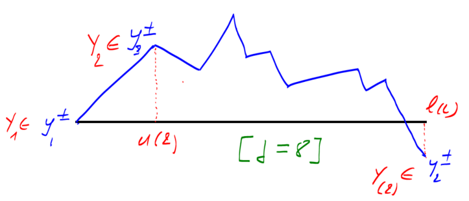
Figure 1. First lower and upper record times, where $Y_{2}$ is an upper record value

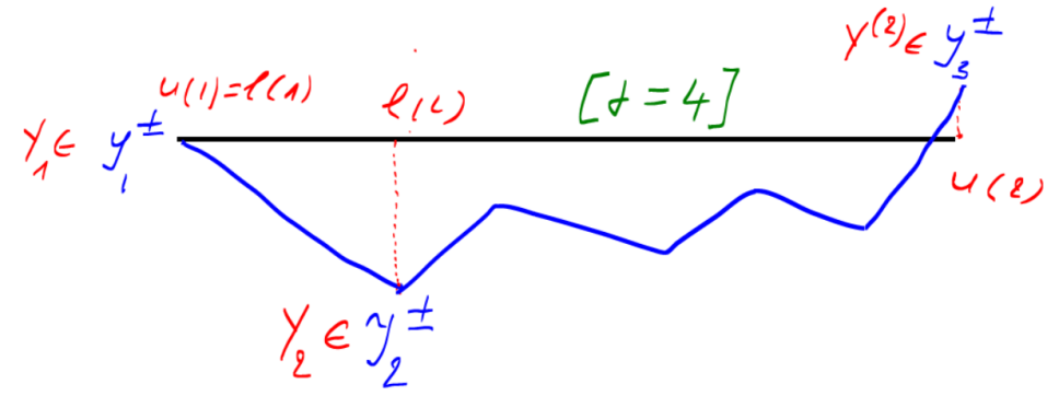
Figure 2. First lower and upper record times, where $Y_{2}$ is a lower record value

Let $N$ be the inter-record time between the two second record times. On $H_{1}=(A(dy)\cap(u(2)<\ell(2))$, for $dy_{i}$ with small norm enough, as illustrated in Fig. 1, we have that $y_{2}<y_{1}<y_{3}$ and for

$$G_{0}=\biggr{(}Y_{1}\in y_{1}^{\pm},\ Y_{2}\in y_{3}^{\pm},\ Y_{3}\in y_{2}^{\pm}\biggr{)},$$

we have

$$(\omega\in H_{1})\cap(N=0)\Rightarrow(\omega\in G_{0}),$$

and for $j\geq 1$,

$$(\omega\in H_{1})\cap(N=j) \Rightarrow \biggr{(}\omega\in(Y_{1}\in y_{1}^{\pm})\bigcap(Y_{2}\in y_{3}^{\pm})\cap(Y_{2+h}\geq y_{1}^{+},\ 1\leq h\leq j)$$

$$\ \ \ \bigcap\ \ (Y_{3+j}\in y_{2}^{\pm})\biggr{)}.$$

Conversely, for $y_{2}<y_{1}<y_{3}$, for

$$G_{j}=(Y_{1}\in y_{1}^{\pm})\cap(Y_{2}\in y_{3}^{\pm})\cap(Y_{2+j}\geq y_{1}^{+},\ 1\leq h\leq j)\cap(Y_{3+j}\in y_{2}^{\pm}),\ j\geq 1,$$

we have for any $j\geq 0$, $\omega\in G_{j}$ implies that $\omega\in A(dy)\cap(N=j)\cap(u(2)<\ell(2))$ and hence

$$G_{j}=H_{1}\cap(N=j),\ j\geq 0.$$

But

$$\mathbb{P}(G_{j})=(F(y_{1}^{+})-F(y_{1}^{-})((F(y_{3}^{+})-F(y_{3}^{-}))(1-F(y_{1}^{+}))^{j}(F(y_{2}^{+})-F(y_{2}^{-})),\ j\geq 0.$$

Finally we have

$$\frac{\mathbb{P}(H_{1})}{\Delta}=\sum_{j\geq 0}\frac{\mathbb{P}(G_{j})}{\Delta}\rightarrow\frac{f(y_{1})f(y_{2})f(y_{3})}{F(y_{1})}1_{(y_{2}<y_{1}<y_{3})}.$$

We treat $(\omega\in H_{2})\cap(N=j)$ in the same manner (see Fig. 2) where $H_{2}=(A(dy)\cap(u(2)>\ell(2))$ and the $G_{j}$’s are replaced by, for $y_{2}<y_{1}<y_{3}$,

$$G_{0}=\biggr{(}Y_{1}\in y_{1}^{\pm},\ Y_{2}\in y_{2}^{\pm},\ Y_{3}\in y_{3}^{\pm}\biggr{)},$$

and

$$G_{j}=(Y_{1}\in y_{1}^{\pm})\cap(Y_{2}\in y_{2}^{\pm})\cap(Y_{2+j}\leq y_{1}^{-},\ 1\leq h\leq j)\cap(Y_{3+j}\in y_{3}^{\pm}),\ j\geq 1,$$

and

$$\mathbb{P}(G_{j})=(F(y_{1}^{+})-F(y_{1}^{-}))(F(y_{2}^{+})-F(y_{2}^{-}))(F(y_{1}^{-})^{j}(F(y_{3}^{+})-F(y_{3}^{-})),\ j\geq 0.$$

We conclude that

$$\frac{\mathbb{P}(H_{2})}{\Delta}=\sum_{j\geq 0}\frac{\mathbb{P}(G_{j})}{\Delta}\rightarrow\frac{f(y_{1})f(y_{2})f(y_{3})}{1-F(y_{1})}1_{(y_{2}<y_{1}<y_{3})}.$$

The proof is over. $\blacksquare$

2.1.2. Derivation of known results and of the second record values (lower and upper)

(i) Let us rediscover the law of $\left(Y_{1},Y^{(2)}\right)$ whose pdf is:

$$f_{(Y_{1},Y^{(2)})}(y_{1},y_{3}) = \int f_{Z_{2}}(y_{1},y_{2},y_{3})dy_{2}$$

$$= 1_{(y_{1}<y_{3})}\left(\frac{1}{F(y_{1})}+\frac{1}{1-F(y_{1})}\right)f(y_{1})f(y_{3})\int_{-\infty}^{y_{1}}\ f(y_{2})dy_{2}$$

$$= 1_{(y_{1}<y_{3})}\left(\frac{1}{F(y_{1})}+\frac{1}{1-F(y_{1})}\right)f(y_{1})f(y_{3})F(y_{1})$$

$$= 1_{(y_{1}<y_{3})}\left(1+\frac{F(y_{1})}{1-F(y_{1})}\right)f(y_{1})f(y_{3})$$

$$= \frac{f(y_{1})}{1-F(y_{1})}f(y_{3})1_{(y_{1}<y_{3})}.$$

So, if $r(x)=f(x)/(1-F(x))$, $x\in]\textit{\text{lep}}(F),\ \textit{\text{uep}}(F)[$, then

$$f_{(Y_{1},Y^{(2)})}(x,y)=r(x)f(y)1_{(x<y)}$$

and this confirms a known result.

(ii) We can derive the law of $\left(Y_{(2)},Y^{(2)}\right)$ as given below:

Corollary 1.

The pdf of $\left(Y_{(2)},Y^{(2)}\right)$ is then

$$f_{(Y_{(2)},Y^{(2)})}(y,z)=f(y)f(z)\left(\log\frac{F(z)}{F(y)}+\log\frac{1-F(y)}{1-F(z)}\right)1_{(y<z)}.$$

Proof of Corollary 1. We have

$$f_{(Y_{(2)},Y^{(2)})}(y_{2},y_{3}) = \int f_{Z_{2}}(y_{1},y_{2},y_{3})dy_{1}$$

$$= 1_{(y_{2}<y_{3})}f(y_{2})f(y_{3})\int_{y_{2}}^{y_{3}}\left(\frac{f(y_{1})}{F(y_{1})}+\frac{f(y_{1})}{1-F(y_{1})}\right)dy_{1}$$

$$= f(y_{2})f(y_{3})\left((R_{1}(y_{3})-R_{1}(y_{2}))+(R_{2}(y_{3})-R_{2}(y_{2}))\right)1_{(y_{2}<y_{3})},$$

with $R_{1}(t)=\log F(t)$  and  $R_{2}(t)=-\log(1-F(t))$. So we finally have

$$f_{(Y_{(2)},Y^{(2)})}(y,z)=f(y)f(z)\left(\log\frac{F(z)}{F(y)}+\log\frac{1-F(y)}{1-F(z)}\right)1_{(y<z)}$$

and the proof is over. $\blacksquare$

2.2. Probability law of the simultaneous joint lower-upper up to three records

2.2.1. Finding the pdf of $Z_{3}$

Proposition 2.

Let $Y_{1}$, $Y_{2}$, $\cdots$ be a sequence of independent real random variables defined on the same probability space $\left(\Omega,\mathcal{A},\mathbb{P}\right)$ with common pdf $f$ and suppose that $u(3)$ and $\ell(3)$ are finite. Then $Z_{3}$ has the following pdf:

$$f_{Z_{3}}(x,y_{1},y_{2},z_{1},z_{2})=f(x)f(y_{1})f(y_{2})f(z_{1})f(z_{2})L(x,y_{1},z_{1})1_{(y_{2}<y_{1}<x<z_{1}<z_{2})},$$

for

$$L(x,y_{1},z_{1})$$

$$=\frac{1}{(1-[F(z_{1})-F(x)])F(x)F(y_{1})}$$

$$+\frac{1}{(1-[F(z_{1})-F(x)])(1-[F(z_{1})-F(y_{1})])(1-F(z_{1}))}$$

$$+\frac{1}{(1-[F(z_{1})-F(x)])(1-[F(z_{1})-F(y_{1})])F(y_{1})}$$

$$+\frac{1}{(1-[F(x)-F(y_{1})])(1-[F(z_{1})-F(y_{1})])(1-F(z_{1}))}$$

$$+\frac{1}{(1-[F(x)-F(y_{1})])(1-[F(z_{1})-F(y_{1})])F(y_{1})}$$

$$+\frac{1}{(1-[F(x)-F(y_{1})])(1-F(x))(1-F(z_{1}))}.$$

Proof of Proposition 2. We use similar methods to those in Section 2.1 but the situation a little more complex. We define

$$A(d):=\left(Y_{1}\in x^{\pm},Y_{(2)}\in y_{1}^{\pm},Y_{(3)}\in y_{2}^{\pm},Y^{(2)}\in z_{1}^{\pm},Y^{(3)}\in z_{2}^{\pm}\right),$$

with $d=(dx,dy_{1},dy_{2},dz_{1},dz_{2})$ and $\Delta=dx\times dy_{1}\times dy_{2}\times dz_{1}\times dz_{2}$. We have to consider all the 24 orderings of $(u(2),u(3),\ell(2),\ell(3))$. Fortunately $u(3)$ (resp. $\ell(3)$) cannot come before $u(2)$ (resp. $\ell(2)$). It will remains six orderings

$$O_{1} = (u(2)<u(3)<\ell(2)<\ell(3))$$

$$O_{2} = (u(2)<\ell(2)<\ell(3)<u(3))$$

$$O_{3} = (u(2)<\ell(2)<u(3)<\ell(3))$$

$$O_{4} = (\ell(2)<u(2)<\ell(3)<u(3))$$

$$O_{5} = (\ell(2)<u(2)<u(3)<\ell(3))$$

$$O_{6} = (\ell(2)<\ell(3)<u(2)<u(3)).$$

Let $N(h)$, $h\in\{1,2,3\}$ the three inter-record times. We have to decompose each $H_{i}=A(d)\cap O_{i}$, $i\in\{1,\cdots,6\}$ into

$$H_{i}=\sum_{i_{1}\geq 0,i_{2}\geq 0,i_{3}\geq 0}H_{i}\cap(N(1)=i_{1},N(2)=i_{2},N(3)=i_{3}).$$

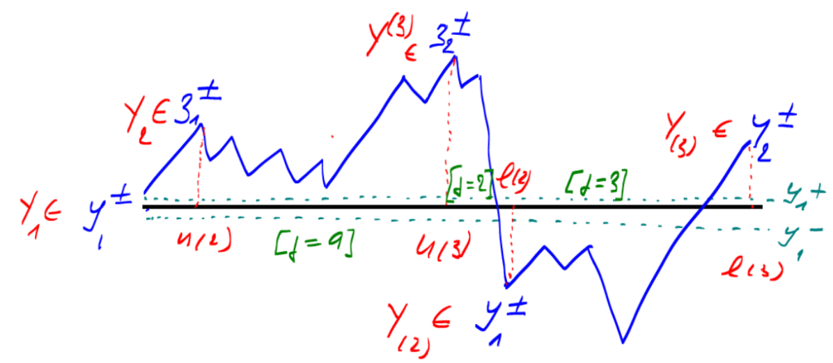
Figure 3. Case $u(2)<u(3)<\ell(2)<\ell(3)$

As above, we are going to describe $G_{i,i_{1},i_{2},i_{3}}=H_{i}\cap(N(1)=i_{1},N(2)=i_{2},N(3)=i_{3})$. We have six cases to deal with. So, we fully explain one cases and let the reader check the other five cases. From Fig. 3, we have the following facts (for $d$ small enough in norm):

(a) For $h\in]u(2),u(3)[$, $Y_{h}>x^{+}$ otherwise it would be the second lower record value, and $Y_{h}<z_{1}^{-}$ otherwise it would be the third upper record;

(b) For $h\in]u(3),\ell(2)[$, $Y_{h}>x^{+}$ otherwise it would be the second lower record (but it may exceed $z_{2}^{+}$ without any consequence);

(c) For $h\in]\ell(2),\ell(3)[$, $Y_{h}>y_{1}^{+}$ otherwise it would be the third lower record (but it is not bounded above).

Hence, we get

$$\frac{\mathbb{P}(G_{1,i_{1},i_{2},i_{3}})}{\Delta}\rightarrow f(x)f(y_{1})f(y_{2})f(z_{1})f(z_{2})(F(z_{1})-F(x))^{i_{1}}(1-F(x))^{i_{2}}(1-F(y_{1}))^{i_{3}},$$

and hence

$$\frac{\mathbb{P}(H_{1})}{\Delta}\rightarrow\frac{f(x)f(y_{1})f(y_{2})f(z_{1})f(z_{2})}{(1-[F(z_{1})-F(x)])F(x)F(y_{1})}.$$

For the five other cases, we have

$$\frac{\mathbb{P}(G_{2,i_{1},i_{2},i_{3}})}{\Delta}\rightarrow f(x)f(y_{1})f(y_{2})f(z_{1})f(z_{2})(F(z_{1})-F(x))^{i_{1}}(F(z_{1})-F(y_{1}))^{i_{2}}F(z_{1})^{i_{3}},$$

$$\frac{\mathbb{P}(G_{3,i_{1},i_{2},i_{3}})}{\Delta}\rightarrow f(x)f(y_{1})f(y_{2})f(z_{1})f(z_{2})(F(z_{1})-F(x))^{i_{1}}(F(z_{1})-F(y_{1}))^{i_{2}}(1-F(y_{1}))^{i_{3}},$$

$$\frac{\mathbb{P}(G_{4,i_{1},i_{2},i_{3}})}{\Delta}\rightarrow f(x)f(y_{1})f(y_{2})f(z_{1})f(z_{2})(F(x)-F(y_{1}))^{i_{1}}(F(z_{1})-F(y_{1}))^{i_{2}}F(z_{1})^{i_{3}},$$

$$\frac{\mathbb{P}(G_{5,i_{1},i_{2},i_{3}})}{\Delta}\rightarrow f(x)f(y_{1})f(y_{2})f(z_{1})f(z_{2})(F(x)-F(y_{1}))^{i_{1}}(F(z_{1})-F(y_{1}))^{i_{2}}(1-F(y_{1}))^{i_{3}},$$

$$\frac{\mathbb{P}(G_{6,i_{1},i_{2},i_{3}})}{\Delta}\rightarrow f(x)f(y_{1})f(y_{2})f(z_{1})f(z_{2})(F(x)-F(y_{1}))^{i_{1}}F(x)^{i_{2}}F(z_{1})^{i_{3}},$$

These facts when put together lead to

$$f_{Z_{3}}(x,y_{1},y_{2},z_{1},z_{2})=f(x)f(y_{1})f(y_{2})f(z_{1})f(z_{2})L(x,y_{1},z_{1})1_{(y_{2}<y_{1}<x<z_{1}<z_{2})}$$

with

$$L(x,y_{1},z_{1})$$

$$=\frac{1}{(1-[F(z_{1})-F(x)])F(x)F(y_{1})}$$

$$+\frac{1}{(1-[F(z_{1})-F(x)])(1-[F(z_{1})-F(y_{1})])(1-F(z_{1}))}$$

$$+\frac{1}{(1-[F(z_{1})-F(x)])(1-[F(z_{1})-F(y_{1})])F(y_{1})}$$

$$+\frac{1}{(1-[F(x)-F(y_{1})])(1-[F(z_{1})-F(y_{1})])(1-F(z_{1}))}$$

$$+\frac{1}{(1-[F(x)-F(y_{1})])(1-[F(z_{1})-F(y_{1})])F(y_{1})}$$

$$+\frac{1}{(1-[F(x)-F(y_{1})])(1-F(x))(1-F(z_{1}))}.$$

2.2.2. Derivation of known results and of the third record values (lower and upper)

(i) Checking of results by comparing with the known pdf of $\left(Y_{1},Y^{(2)},Y^{(3)}\right)$.

We have

$$f_{(Y_{1},Y^{(2)},Y^{(3)})}(x,z_{1},z_{2}) = \int\int f_{Z_{3}}(x,y_{1},y_{2},z_{1},z_{2})dy_{1}dy_{2}$$

$$=: 1_{(x<z_{1}<z_{2})}f(x)f(z_{1})f(z_{2})\left(I_{1}+I_{2}+I_{3}+I_{4}+I_{5}+I_{6}\right).$$

Let us denote, for $(x,z_{1},z_{2})$ fixed, by $D_{x}:=D_{(x,z_{1},z_{2})}=(y_{2}<y_{1}<x)$ as the section of the domain of $Z_{3}$ at $(x,z_{1},z_{2})$. So

$$I_{1} = \int\int_{D_{x}}\frac{f(y_{1})f(y_{2})}{(1-[F(z_{1})-F(x)])F(x)F(y_{1})}dy_{1}dy_{2}$$

$$= \frac{1}{(1-[F(z_{1})-F(x)])F(x)}\int\int_{D_{x}}\frac{f(y_{1})f(y_{2})}{F(y_{1})}dy_{1}dy_{2}$$

$$= \frac{1}{(1-[F(z_{1})-F(x)])F(x)}\int_{-\infty}^{x}\frac{f(y_{1})}{F(y_{1})}\left(\int_{-\infty}^{y_{1}}f(y_{2})dy_{2}\right)dy_{1}$$

$$= \frac{1}{(1-[F(z_{1})-F(x)])}.$$

$$I_{2} = \int\int_{D_{x}}\frac{f(y_{1})f(y_{2})}{(1-[F(z_{1})-F(x)])(1-[F(z_{1})-F(y_{1})])(1-F(z_{1}))}dy_{1}dy_{2}$$

$$= \frac{1}{(1-[F(z_{1})-F(x)])(1-F(z_{1}))}\int\int_{D_{x}}\frac{f(y_{1})f(y_{2})}{1-[F(z_{1})-F(y_{1})]}dy_{1}dy_{2}$$

$$= \frac{1}{(1-[F(z_{1})-F(x)])(1-F(z_{1}))}\int_{-\infty}^{x}\frac{f(y_{1})}{1-[F(z_{1})-F(y_{1})]}\left(\int_{-\infty}^{y_{1}}f(y_{2})dy_{2}\right)dy_{1}$$

$$= \frac{1}{(1-[F(z_{1})-F(x)])(1-F(z_{1}))}\int_{-\infty}^{x}\frac{f(y_{1})F(y_{1})}{1-[F(z_{1})-F(y_{1})]}dy_{1}$$

$$= \frac{1}{(1-[F(z_{1})-F(x)])(1-F(z_{1}))}\int_{-\infty}^{x}\frac{f(y_{1})\left\{1-[F(z_{1})-F(y_{1})]\right\}-f(y_{1})(1-F(z_{1}))}{1-[F(z_{1})-F(y_{1})]}dy_{1}$$

$$= \frac{1}{(1-[F(z_{1})-F(x)])(1-F(z_{1}))}\left\{\int_{-\infty}^{x}f(y_{1})dy_{1}-\int_{-\infty}^{x}\frac{f(y_{1})(1-F(z_{1}))}{1-[F(z_{1})-F(y_{1})]}dy_{1}\right\}$$

$$= \frac{1}{(1-[F(z_{1})-F(x)])(1-F(z_{1}))}\left\{F(x)-(1-F(z_{1}))\log\frac{1-[F(z_{1})-F(x)]}{1-F(z_{1})}\right\}$$

$$= \frac{F(x)}{(1-[F(z_{1})-F(x)])(1-F(z_{1}))}-\frac{\log\left(1-[F(z_{1})-F(x)]\right)-\log\left(1-F(z_{1})\right)}{1-[F(z_{1})-F(x)]}.$$

$$I_{3} = \int\int_{D_{x}}\frac{f(y_{1})f(y_{2})}{(1-[F(z_{1})-F(x)])(1-[F(z_{1})-F(y_{1})])F(y_{1})}dy_{1}dy_{2}$$

$$= \frac{1}{1-[F(z_{1})-F(x)]}\int\int_{D_{x}}\frac{f(y_{1})f(y_{2})}{(1-[F(z_{1})-F(y_{1})])F(y_{1})}dy_{1}dy_{2}$$

$$= \frac{1}{1-[F(z_{1})-F(x)]}\int_{-\infty}^{x}\frac{f(y_{1})}{(1-[F(z_{1})-F(y_{1})])F(y_{1})}\left(\int_{-\infty}^{y_{1}}f(y_{2})dy_{2}\right)dy_{1}$$

$$= \frac{1}{1-[F(z_{1})-F(x)]}\int_{-\infty}^{x}\frac{f(y_{1})}{1-[F(z_{1})-F(y_{1})]}dy_{1}$$

$$= \frac{\log\left(1-[F(z_{1})-F(x)]\right)-\log\left(1-F(z_{1})\right)}{1-[F(z_{1})-F(x)]}.$$

$$I_{4} = \int\int_{D_{x}}\frac{f(y_{1})f(y_{2})}{(1-[F(x)-F(y_{1})])(1-[F(z_{1})-F(y_{1})])(1-F(z_{1}))}dy_{1}dy_{2}$$

$$= \frac{1}{(1-F(z_{1}))}\int\int_{D_{x}}\frac{f(y_{1})f(y_{2})}{(1-[F(x)-F(y_{1})])(1-[F(z_{1})-F(y_{1})])}dy_{1}dy_{2}$$

$$= \frac{1}{(1-F(z_{1}))}\int_{-\infty}^{x}\frac{f(y_{1})}{(1-[F(x)-F(y_{1})])(1-[F(z_{1})-F(y_{1})])}\left(\int_{-\infty}^{y_{1}}f(y_{2})dy_{2}\right)dy_{1}$$

$$= \frac{1}{(1-F(z_{1}))}\int_{-\infty}^{x}\frac{f(y_{1})F(y_{1})}{(1-[F(x)-F(y_{1})])(1-[F(z_{1})-F(y_{1})])}dy_{1}.$$

Hence we use the following decomposition

$$\frac{F(y_{1})}{(1-[F(x)-F(y_{1})])(1-[F(z_{1})-F(y_{1})])} = \frac{1-F(z_{1})}{F(x)-F(z_{1})}\times\frac{1}{1-[F(z_{1})-F(y_{1})]}$$

$$- \frac{1-F(x)}{F(x)-F(z_{1})}\times\frac{1}{1-[F(x)-F(y_{1})]}$$

and so

$$I_{4} = \frac{1}{(1-F(z_{1}))}\biggr{(}\frac{1-F(z_{1})}{F(x)-F(z_{1})}\int_{-\infty}^{x}\frac{f(y_{1})}{1-[F(z_{1})-F(y_{1})]}dy_{1}$$

$$- \frac{1-F(x)}{F(x)-F(z_{1})}\int_{-\infty}^{x}\frac{f(y_{1})}{1-[F(x)-F(y_{1})]}dy_{1}\biggr{)}$$

$$= \frac{1}{(1-F(z_{1}))}\biggr{(}\frac{1-F(z_{1})}{F(x)-F(z_{1})}\left(\log\left(1-[F(z_{1})-F(x)]\right)-\log\left(1-F(z_{1})\right)\right)$$

$$+ \frac{1-F(x)}{F(x)-F(z_{1})}\log\left(1-F(x)\right)\biggr{)}$$

$$= \frac{1}{(1-F(z_{1}))(F(x)-F(z_{1}))}\biggr{(}(1-F(z_{1}))\biggr{(}\log\left(1-[F(z_{1})-F(x)]\right)-\log\left(1-F(z_{1})\right)\biggr{)}$$

$$+ (1-F(x))\log\left(1-F(x)\right)\biggr{)}.$$

$$I_{5} = \int\int_{D_{x}}\frac{f(y_{1})f(y_{2})}{(1-[F(x)-F(y_{1})])(1-[F(z_{1})-F(y_{1})])F(y_{1})}dy_{1}dy_{2}$$

$$= \int_{-\infty}^{x}\frac{f(y_{1})}{(1-[F(x)-F(y_{1})])(1-[F(z_{1})-F(y_{1})])F(y_{1})}\left(\int_{-\infty}^{y_{1}}f(y_{2})dy_{2}\right)dy_{1}$$

$$= \int_{-\infty}^{x}\frac{f(y_{1})}{(1-[F(x)-F(y_{1})])(1-[F(z_{1})-F(y_{1})])}dy_{1}$$

$$= \frac{1}{F(x)-F(z_{1})}\int_{-\infty}^{x}\frac{f(y_{1})(F(x)-F(z_{1}))}{(1-[F(x)-F(y_{1})])(1-[F(z_{1})-F(y_{1})])}dy_{1}$$

$$= \frac{1}{F(x)-F(z_{1})}\biggr{(}\int_{-\infty}^{x}\frac{f(y_{1})}{1-[F(x)-F(y_{1})]}dy_{1}-\int_{-\infty}^{x}\frac{f(y_{1})}{1-[F(z_{1})-F(y_{1})]}dy_{1}\biggr{)}\ (L4)$$

$$= \frac{\log\left(1-F(z_{1})\right)-\log\left(1-F(x)\right)-\log\left(1-[F(z_{1})-F(x)]\right)}{F(x)-F(z_{1})}$$

where we used in Line (L4) the simple fact

$$\frac{(F(x)-F(z_{1}))}{(1-[F(x)-F(y_{1})])(1-[F(z_{1})-F(y_{1})])}=\frac{1}{1-[F(x)-F(y_{1})]}-\frac{1}{1-[F(z_{1})-F(y_{1})]}$$

$$I_{6} = \int\int_{D_{x}}\frac{f(y_{1})f(y_{2})}{(1-[F(x)-F(y_{1})])(1-F(x))(1-F(z_{1}))}dy_{1}dy_{2}$$

$$= \frac{1}{(1-F(x))(1-F(z_{1}))}\int\int_{D_{x}}\frac{f(y_{1})f(y_{2})}{1-[F(x)-F(y_{1})]}dy_{1}dy_{2}$$

$$= \frac{1}{(1-F(x))(1-F(z_{1}))}\int_{-\infty}^{x}\frac{f(y_{1})}{1-[F(x)-F(y_{1})]}\left(\int_{-\infty}^{y_{1}}f(y_{2})dy_{2}\right)dy_{1}$$

$$= \frac{1}{(1-F(x))(1-F(z_{1}))}\int_{-\infty}^{x}\frac{f(y_{1})F(y_{1})}{1-[F(x)-F(y_{1})]}dy_{1}$$

$$= \frac{1}{(1-F(x))(1-F(z_{1}))}\biggr{(}\int_{-\infty}^{x}f(y_{1})dy_{1}$$

$$- \int_{-\infty}^{x}(1-F(x))\frac{f(y_{1})}{1-[F(x)-F(y_{1})]}dy_{1}\biggr{)}$$

$$= \frac{1}{(1-F(x))(1-F(z_{1}))}\biggr{(}F(x)+(1-F(x))\log(1-F(x))\biggr{)}$$

$$= \frac{F(x)}{(1-F(x))(1-F(z_{1}))}+\frac{\log(1-F(x))}{1-F(z_{1})}$$

Hence by doing the simple computations, we arrive at

$$I_{1}+I_{2}+I_{3}+I_{4}+I_{5}+I_{6}=\frac{1}{(1-F(x))(1-F(z_{1}))}$$

and hence

$$f_{(Y_{1},Y^{(2)},Y^{(3)})}(x,z_{1},z_{2}) = \frac{f(x)f(z_{1})f(z_{2})}{(1-F(x))(1-F(z_{1}))}1_{(x<z_{1}<z_{2})}$$

$$= r(x)r(z_{1})f(z_{2})1_{(x<z_{1}<z_{2})}$$

and this confirms a known result, with

$$r(t)=f(t)/(1-F(t)),\ \ t\in]\textit{\text{lep}}(F),\ \textit{\text{uep}}(F)[.$$

(ii) Let us derive the laws of $\left(Y_{(p)},Y^{(q)}\right)$, $2\leq p,q\leq 3$.

Let us begin by checking the law of $\left(Y_{(2)},Y^{(2)}\right)$, which has already been found in Corollary 1.

We have

$$f_{(Y_{(2)},Y^{(2)})}(y_{1},z_{1}) = \int\int\int f_{Z_{3}}(x,y_{1},y_{2},z_{1},z_{2})dxdy_{2}dz_{2}$$

$$=: 1_{(y_{1}<z_{1})}f(y_{1})f(z_{1})\left(J_{1}+J_{2}+J_{3}+J_{4}+J_{5}+J_{6}\right).$$

Let us denote by, for $(y_{1},z_{1})$ fixed, $D_{(y_{1},z_{1})}=(y_{2}<y_{1}<x<z_{1}<z_{2})=:D_{x}$ as the section of the domain of $Z_{3}$ at $(y_{1},z_{1})$ . So

$$J_{1} = \int\int\int_{D_{x}}\frac{f(x)f(y_{2})f(z_{2})}{(1-[F(z_{1})-F(x)])F(x)F(y_{1})}dxdy_{2}dz_{2}$$

$$= \frac{1}{F(y_{1})}\int_{-\infty}^{y_{1}}f(y_{2})dy_{2}\int_{z_{1}}^{+\infty}f(z_{2})dz_{2}\int_{y_{1}}^{z_{1}}\frac{f(x)}{(1-[F(z_{1})-F(x)])F(x)}dx$$

$$= \int_{y_{1}}^{z_{1}}\frac{f(x)(1-F(z_{1}))}{(1-[F(z_{1})-F(x)])F(x)}dx.$$

But remark that

$$\frac{1-F(z_{1})}{(1-[F(z_{1})-F(x)])F(x)}=\frac{1}{F(x)}-\frac{1}{1-[F(z_{1})-F(x)]}$$

and hence

$$J_{1} = \int_{y_{1}}^{z_{1}}\biggr{(}\frac{f(x)}{F(x)}-\frac{f(x)}{1-[F(z_{1})-F(x)]}\biggr{)}dx$$

$$= \log\frac{F(z_{1})}{F(y_{1})}+\log\left(1-[F(z_{1})-F(y_{1})]\right).$$

$$J_{2} = \int\int\int_{D_{x}}\frac{f(x)f(y_{2})f(z_{2})}{(1-[F(z_{1})-F(x)])(1-[F(z_{1})-F(y_{1})])(1-F(z_{1}))}dxdy_{2}dz_{2}$$

$$= \frac{1}{(1-[F(z_{1})-F(y_{1})])(1-F(z_{1}))}\int_{-\infty}^{y_{1}}f(y_{2})dy_{2}$$

$$\int_{z_{1}}^{+\infty}f(z_{2})dz_{2}\int_{y_{1}}^{z_{1}}\frac{f(x)}{1-[F(z_{1})-F(x)]}dx$$

$$= -F(y_{1})\times\frac{\log\left(1-[F(z_{1})-F(y_{1})]\right)}{1-[F(z_{1})-F(y_{1})]}.$$

$$J_{3} = \int\int\int_{D_{x}}\frac{f(x)f(y_{2})f(z_{2})}{(1-[F(z_{1})-F(x)])(1-[F(z_{1})-F(y_{1})])F(y_{1})}dxdy_{2}dz_{2}$$

$$= \frac{1}{(1-[F(z_{1})-F(y_{1})])F(y_{1})}\int_{-\infty}^{y_{1}}f(y_{2})dy_{2}$$

$$\int_{z_{1}}^{+\infty}f(z_{2})dz_{2}\int_{y_{1}}^{z_{1}}\frac{f(x)}{1-[F(z_{1})-F(x)]}dx$$

$$= -(1-F(z_{1}))\times\frac{\log\left(1-[F(z_{1})-F(y_{1})]\right)}{1-[F(z_{1})-F(y_{1})]}.$$

$$J_{4} = \int\int\int_{D_{x}}\frac{f(x)f(y_{2})f(z_{2})}{(1-[F(x)-F(y_{1})])(1-[F(z_{1})-F(y_{1})])(1-F(z_{1}))}dxdy_{2}dz_{2}$$

$$= \frac{1}{(1-[F(z_{1})-F(y_{1})])(1-F(z_{1}))}\int_{-\infty}^{y_{1}}f(y_{2})dy_{2}\int_{z_{1}}^{+\infty}f(z_{2})dz_{2}$$

$$\int_{y_{1}}^{z_{1}}\frac{f(x)}{1-[F(x)-F(y_{1})]}dx$$

$$= -F(y_{1})\times\frac{\log\left(1-[F(z_{1})-F(y_{1})]\right)}{1-[F(z_{1})-F(y_{1})]}.$$

$$J_{5} = \int\int\int_{D_{x}}\frac{f(x)f(y_{2})f(z_{2})}{(1-[F(x)-F(y_{1})])(1-[F(z_{1})-F(y_{1})])F(y_{1})}dxdy_{2}dz_{2}$$

$$= \frac{1}{(1-[F(z_{1})-F(y_{1})])F(y_{1})}\int_{-\infty}^{y_{1}}f(y_{2})dy_{2}$$

$$\int_{z_{1}}^{+\infty}f(z_{2})dz_{2}\int_{y_{1}}^{z_{1}}\frac{f(x)}{1-[F(x)-F(y_{1})]}dx$$

$$= -(1-F(z_{1}))\times\frac{\log\left(1-[F(z_{1})-F(y_{1})]\right)}{1-[F(z_{1})-F(y_{1})]}.$$

$$J_{6} = \int\int\int_{D_{x}}\frac{f(x)f(y_{2})f(z_{2})}{(1-[F(x)-F(y_{1})])(1-F(x))(1-F(z_{1}))}dxdy_{2}dz_{2}$$

$$= \frac{1}{(1-F(z_{1}))}\int_{-\infty}^{y_{1}}f(y_{2})dy_{2}\int_{z_{1}}^{+\infty}f(z_{2})dz_{2}$$

$$\int_{y_{1}}^{z_{1}}\frac{f(x)}{(1-[F(x)-F(y_{1})])(1-F(x))}dx$$

$$= \int_{y_{1}}^{z_{1}}\frac{f(x)F(y_{1})}{(1-[F(x)-F(y_{1})])(1-F(x))}dx.$$

But remark that

$$\frac{F(y_{1})}{(1-[F(x)-F(y_{1})])(1-F(x))}=\frac{1}{1-F(x)}-\frac{1}{1-[F(x)-F(y_{1})]}$$

and hence

$$J_{6} = \int_{y_{1}}^{z_{1}}\biggr{(}\frac{f(x)}{1-F(x)}-\frac{f(x)}{1-[F(x)-F(y_{1})]}\biggr{)}dx$$

$$= \log\frac{1-F(y_{1})}{1-F(z_{1})}+\log\left(1-[F(z_{1})-F(y_{1})]\right).$$

Hence by regrouping all terms, we will have

$$f_{(Y_{(2)},Y^{(2)})}(y_{1},z_{1})=f(y_{1})f(z_{1})\left(\log\frac{F(z_{1})}{F(y_{1})}+\log\frac{1-F(y_{1})}{1-F(z_{1})}\right)1_{(y_{1}<z_{1})}$$

and that confirms the result found in Corollary 1.

Now, we are going to derive the laws of $\left(Y_{(2)},Y^{(3)}\right)$, $\left(Y_{(3)},Y^{(2)}\right)$ and $\left(Y_{(3)},Y^{(3)}\right)$ in the next Corollaries.

Corollary 2.

The pdf of $\left(Y_{(2)},Y^{(3)}\right)$ is then given by

$$f_{(Y_{(2)},Y^{(3)})}(y,z)=-f(y)f(z)\biggr{(}\int_{y}^{z}\frac{f(x)}{F(x)(1-F(x))}\log\frac{1-F(z)}{1-F(x)}dx\biggr{)}1_{(y<z)}.$$

Proof of Corollary 2. We have

$$f_{(Y_{(2)},Y^{(3)})}(y_{1},z_{2}) = \int\int\int f_{Z_{3}}(x,y_{1},y_{2},z_{1},z_{2})dxdy_{2}dz_{1}$$

$$=: 1_{(y_{1}<z_{2})}f(y_{1})f(z_{2})\left(K_{1}+K_{2}+K_{3}+K_{4}+K_{5}+K_{6}\right).$$

Let us denote, for $(y_{1},z_{2})$ fixed, by $D_{(y_{1},z_{2})}=(y_{2}<y_{1}<x<z_{1}<z_{2})=:D_{x}$ as the section of the domain of $Z_{3}$ at $(y_{1},z_{2})$. So

$$K_{1} = \int\int\int_{D_{x}}\frac{f(x)f(y_{2})f(z_{1})}{(1-[F(z_{1})-F(x)])F(x)F(y_{1})}dxdy_{2}dz_{1}$$

$$= \frac{1}{F(y_{1})}\int_{-\infty}^{y_{1}}f(y_{2})dy_{2}\int_{y_{1}}^{z_{2}}\frac{f(x)}{F(x)}\biggr{(}\int_{x}^{z_{2}}\frac{f(z_{1})}{(1-[F(z_{1})-F(x)])}dz_{1}\biggr{)}dx$$

$$= -\int_{y_{1}}^{z_{2}}\frac{f(x)}{F(x)}\log\left(1-[F(z_{2})-F(x)]\right)dx.$$

$$K_{2} = \int\int\int_{D_{x}}\frac{f(x)f(y_{2})f(z_{1})}{(1-[F(z_{1})-F(x)])(1-[F(z_{1})-F(y_{1})])(1-F(z_{1}))}dxdy_{2}dz_{1}$$

$$= \int_{-\infty}^{y_{1}}f(y_{2})dy_{2}\int_{y_{1}}^{z_{2}}f(x)$$

$$\biggr{(}\int_{x}^{z_{2}}\frac{f(z_{1})}{(1-[F(z_{1})-F(x)])(1-[F(z_{1})-F(y_{1})])(1-F(z_{1}))}dz_{1}\biggr{)}dx$$

$$= F(y_{1})\int_{y_{1}}^{z_{2}}f(x)$$

$$\biggr{(}\int_{x}^{z_{2}}\frac{f(z_{1})}{(1-[F(z_{1})-F(x)])(1-[F(z_{1})-F(y_{1})])(1-F(z_{1}))}dz_{1}\biggr{)}dx.$$

Now we use the following relation

$$\frac{1}{(1-[F(z_{1})-F(x)])(1-[F(z_{1})-F(y_{1})])(1-F(z_{1}))}$$

$$=\frac{1}{F(x)(F(y_{1})-F(x))}\biggr{(}\frac{1}{1-F(z_{1})}-\frac{1}{1-[F(z_{1})-F(x)]}\biggr{)}$$

$$-\frac{1}{F(y_{1})(F(y_{1})-F(x))}\biggr{(}\frac{1}{1-F(z_{1})}-\frac{1}{1-[F(z_{1})-F(y_{1})]}\biggr{)}.$$

to get

$$K_{2} = F(y_{1})\int_{y_{1}}^{z_{2}}\frac{f(x)}{F(x)(F(y_{1})-F(x))}\biggr{(}\left\{\frac{f(z_{1})}{1-F(z_{1})}-\frac{f(z_{1})}{1-[F(z_{1})-F(x)]}\right\}dz_{1}\biggr{)}dx$$

$$- F(y_{1})\int_{y_{1}}^{z_{2}}\frac{f(x)}{F(y_{1})(F(y_{1})-F(x))}\biggr{(}\left\{\frac{f(z_{1})}{1-F(z_{1})}-\frac{f(z_{1})}{1-[F(z_{1})-F(y_{1})]}\right\}dz_{1}\biggr{)}dx$$

$$= \int_{y_{1}}^{z_{2}}\frac{f(x)F(y_{1})}{F(x)(F(y_{1})-F(x))}\biggr{(}-\log\frac{1-F(z_{2})}{1-F(x)}+\log\left(1-[F(z_{2})-F(x)]\right)\biggr{)}dx$$

$$- \int_{y_{1}}^{z_{2}}\frac{f(x)}{F(y_{1})-F(x)}\biggr{(}-\log\frac{1-F(z_{2})}{1-F(x)}+\log\frac{1-[F(z_{2})-F(y_{1})]}{1-[F(x)-F(y_{1})]}\biggr{)}dx$$

$$= -\int_{y_{1}}^{z_{2}}\frac{f(x)F(y_{1})}{F(x)(F(y_{1})-F(x))}\log\frac{1-F(z_{2})}{1-F(x)}dx$$

$$+ \int_{y_{1}}^{z_{2}}\frac{f(x)F(y_{1})}{F(x)(F(y_{1})-F(x))}\log\left(1-[F(z_{2})-F(x)]\right)dx$$

$$+ \int_{y_{1}}^{z_{2}}\frac{f(x)}{F(y_{1})-F(x)}\log\frac{1-F(z_{2})}{1-F(x)}dx$$

$$- \int_{y_{1}}^{z_{2}}\frac{f(x)}{F(y_{1})-F(x)}\log\frac{1-[F(z_{2})-F(y_{1})]}{1-[F(x)-F(y_{1})]}dx.$$

$$K_{3} = \int\int\int_{D_{x}}\frac{f(x)f(y_{2})f(z_{1})}{(1-[F(z_{1})-F(x)])(1-[F(z_{1})-F(y_{1})])F(y_{1})}dxdy_{2}dz_{1}$$

$$= \frac{1}{F(y_{1})}\int_{-\infty}^{y_{1}}f(y_{2})dy_{2}\int_{y_{1}}^{z_{2}}f(x)$$

$$\biggr{(}\int_{x}^{z_{2}}\frac{f(z_{1})}{(1-[F(z_{1})-F(x)])(1-[F(z_{1})-F(y_{1})])}dz_{1}\biggr{)}dx$$

$$= \int_{y_{1}}^{z_{2}}\frac{f(x)}{F(y_{1})-F(x)}\biggr{(}\int_{x}^{z_{2}}\left\{\frac{f(z_{1})}{1-[F(z_{1})-F(x)]}-\frac{f(z_{1})}{1-[F(z_{1})-F(y_{1})]}\right\}dz_{1}\biggr{)}dx$$

$$= -\int_{y_{1}}^{z_{2}}\frac{f(x)}{F(y_{1})-F(x)}\log\left(1-[F(z_{2})-F(x)]\right)dx$$

$$+ \int_{y_{1}}^{z_{2}}\frac{f(x)}{F(y_{1})-F(x)}\log\frac{1-[F(z_{2})-F(y_{1})]}{1-[F(x)-F(y_{1})]}dx.$$

$$K_{4} = \int\int\int_{D_{x}}\frac{f(x)f(y_{2})f(z_{1})}{(1-[F(x)-F(y_{1})])(1-[F(z_{1})-F(y_{1})])(1-F(z_{1}))}dxdy_{2}dz_{1}$$

$$= \int_{-\infty}^{y_{1}}f(y_{2})dy_{2}\int_{y_{1}}^{z_{2}}\frac{f(x)}{1-[F(x)-F(y_{1})]}$$

$$\biggr{(}\int_{x}^{z_{2}}\frac{f(z_{1})}{(1-[F(z_{1})-F(y_{1})])(1-F(z_{1}))}dz_{1}\biggr{)}dx$$

$$= \int_{y_{1}}^{z_{2}}\frac{f(x)}{1-[F(x)-F(y_{1})]}\biggr{(}\int_{x}^{z_{2}}\left\{\frac{f(z_{1})}{1-F(z_{1})}dz_{1}-\frac{f(z_{1})}{1-[F(z_{1})-F(y_{1})]}\right\}dz_{1}\biggr{)}dx$$

$$= \int_{y_{1}}^{z_{2}}\frac{f(x)}{1-[F(x)-F(y_{1})]}\biggr{(}-\log\frac{1-F(z_{2})}{1-F(x)}+\log\frac{1-[F(z_{2})-F(y_{1})]}{1-[F(x)-F(y_{1})]}\biggr{)}dx$$

$$= -\int_{y_{1}}^{z_{2}}\frac{f(x)}{1-[F(x)-F(y_{1})]}\log\frac{1-F(z_{2})}{1-F(x)}dx$$

$$+ \int_{y_{1}}^{z_{2}}\frac{f(x)}{1-[F(x)-F(y_{1})]}\log\frac{1-[F(z_{2})-F(y_{1})]}{1-[F(x)-F(y_{1})]}dx.$$

$$K_{5} = \int\int\int_{D_{x}}\frac{f(x)f(y_{2})f(z_{1})}{(1-[F(x)-F(y_{1})])(1-[F(z_{1})-F(y_{1})])F(y_{1}}dxdy_{2}dz_{1}$$

$$= \frac{1}{F(y_{1})}\int_{-\infty}^{y_{1}}f(y_{2})dy_{2}\int_{y_{1}}^{z_{2}}\frac{f(x)}{1-[F(x)-F(y_{1})]}\biggr{(}\int_{x}^{z_{2}}\frac{f(z_{1})}{1-[F(z_{1})-F(y_{1})]}dz_{1}\biggr{)}dx$$

$$= -\int_{y_{1}}^{z_{2}}\frac{f(x)}{1-[F(x)-F(y_{1})]}\log\frac{1-[F(z_{2})-F(y_{1})]}{1-[F(x)-F(y_{1})]}dx.$$

$$K_{6} = \int\int\int_{D_{x}}\frac{f(x)f(y_{2})f(z_{1})}{(1-[F(x)-F(y_{1})])(1-F(x))(1-F(z_{1})])}dxdy_{2}dz_{1}$$

$$= \int_{-\infty}^{y_{1}}f(y_{2})dy_{2}\int_{y_{1}}^{z_{2}}\frac{f(x)}{(1-F(x))(1-[F(x)-F(y_{1}))]}\biggr{(}\int_{x}^{z_{2}}\frac{f(z_{1})}{1-F(z_{1})}dz_{1}\biggr{)}dx$$

$$= -\int_{y_{1}}^{z_{2}}\frac{f(x)F(y_{1})}{(1-F(x))(1-[F(x)-F(y_{1}))]}\log\frac{1-F(z_{2})}{1-F(x)}dx.$$

Hence by regrouping all terms, we show that

$$K_{1}+K_{2}+K_{3}+K_{4}+K_{5}+K_{6}$$

$$=-\int_{y_{1}}^{z_{2}}\frac{f(x)}{F(x)(1-F(x))}\log\frac{1-F(z_{2})}{1-F(x)}dx$$

and this finishes the proof. $\blacksquare$

Corollary 3.

The pdf of $\left(Y_{(3)},Y^{(2)}\right)$ is then given by

$$f_{(Y_{(3)},Y^{(2)})}(y,z)=-f(y)f(z)\biggr{(}\int_{y}^{z}\frac{f(x)}{F(x)(1-F(x))}\log\frac{F(y)}{F(x)}dx\biggr{)}1_{(y<z)}.$$

Proof of Corollary 3. We have

$$f_{(Y_{(3)},Y^{(2)})}(y_{2},z_{1}) = \int\int\int f_{Z_{3}}(x,y_{1},y_{2},z_{1},z_{2})dxdy_{1}dz_{2}$$

$$=: 1_{(y_{2}<z_{1})}f(y_{2})f(z_{1})\left(M_{1}+M_{2}+M_{3}+M_{4}+M_{5}+M_{6}\right).$$

Let us denote by, for $(y_{2},z_{1})$ fixed, $D_{(y_{2},z_{1})}=(y_{2}<y_{1}<x<z_{1}<z_{2})=:D_{x}$ as the section of the domain of $Z_{3}$ at $(y_{2},z_{1})$ . So

$$M_{1} = \int\int\int_{D_{x}}\frac{f(x)f(z_{2})f(y_{1})}{(1-[F(z_{1})-F(x)])F(x)F(y_{1})}dxdz_{2}dy_{1}$$

$$= \frac{1}{F(y_{1})}\int_{z_{1}}^{+\infty}f(z_{2})dz_{2}\int_{y_{2}}^{z_{1}}\frac{f(x)}{F(x)(1-[F(z_{1})-F(x)])}$$

$$\biggr{(}\int_{y_{2}}^{x}\frac{f(y_{1})}{F(y_{1})}dy_{1}\biggr{)}dx$$

$$= (1-F(z_{1}))\int_{y_{2}}^{z_{1}}\frac{f(x)}{F(x)(1-[F(z_{1})-F(x)])}\log\frac{F(x)}{F(y_{2})}dx.$$

$$M_{2} = \int\int\int_{D_{x}}\frac{f(x)f(z_{2})f(y_{1})}{(1-[F(z_{1})-F(x)])(1-[F(z_{1})-F(y_{1})])(1-F(z_{1}))}dxdz_{2}dy_{1}$$

$$= \frac{1}{1-F(z_{1})}\int_{z_{1}}^{+\infty}f(z_{2})dz_{2}\int_{y_{2}}^{z_{1}}\frac{f(x)}{1-[F(z_{1})-F(x)]}$$

$$\biggr{(}\int_{y_{2}}^{x}\frac{f(y_{1})}{1-[F(z_{1})-F(y_{1})]}dy_{1}\biggr{)}dx$$

$$= \int_{y_{2}}^{z_{1}}\frac{f(x)}{F(x)(1-[F(z_{1})-F(x)])}\log\frac{1-[F(z_{1})-F(x)]}{1-[F(z_{1})-F(y_{2})]}dx.$$

$$M_{3} = \int\int\int_{D_{x}}\frac{f(x)f(z_{2})f(y_{1})}{(1-[F(z_{1})-F(x)])(1-[F(z_{1})-F(y_{1})])F(y_{1})}dxdz_{2}dy_{1}$$

$$= \int_{z_{1}}^{+\infty}f(z_{2})dz_{2}\int_{y_{2}}^{z_{1}}\frac{f(x)}{1-[F(z_{1})-F(x)]}$$

$$\biggr{(}\int_{y_{2}}^{x}\frac{f(y_{1})}{(1-[F(z_{1})-F(y_{1}))F(y_{1})]}dy_{1}\biggr{)}dx$$

$$= \int_{y_{2}}^{z_{1}}\frac{f(x)}{1-[F(z_{1})-F(x)]}\biggr{(}\int_{y_{2}}^{x}\left\{\frac{f(y_{1})}{F(y_{1})}-\frac{f(y_{1})}{1-[F(z_{1})-F(y_{1})]}\right\}dy_{1}\biggr{)}dx$$

$$= \int_{y_{2}}^{z_{1}}\frac{f(x)}{1-[F(z_{1})-F(x)]}\log\frac{F(x)}{F(y_{2})}dx$$

$$- \int_{y_{2}}^{z_{1}}\frac{f(x)}{1-[F(z_{1})-F(x)]}\log\frac{1-[F(z_{1})-F(x)]}{1-[F(z_{1})-F(y_{2})]}dx.$$

$$M_{4} = \int\int\int_{D_{x}}\frac{f(x)f(z_{2})f(y_{1})}{(1-[F(x)-F(y_{1})])(1-[F(z_{1})-F(y_{1})])(1-F(z_{1}))}dxdz_{2}dy_{1}$$

$$= \frac{1}{1-F(z_{1})}\int_{z_{1}}^{+\infty}f(z_{2})dz_{2}\int_{y_{2}}^{z_{1}}f(x)$$

$$\biggr{(}\int_{y_{2}}^{x}\frac{f(y_{1})}{(1-[F(x)-F(y_{1})])(1-[F(z_{1})-F(y_{1})])}dy_{1}\biggr{)}dx$$

$$= \int_{y_{2}}^{z_{1}}\frac{f(x)}{F(z_{1})-F(x)}\biggr{(}\int_{y_{2}}^{x}\left\{\frac{f(y_{1})}{1-[F(z_{1})-F(y_{1})]}-\frac{f(y_{1})}{1-[F(z_{1})-F(y_{1})]}\right\}dy_{1}\biggr{)}dx$$

$$= \int_{y_{2}}^{z_{1}}\frac{f(x)}{F(z_{1})-F(x)}\log\frac{1-[F(z_{1})-F(x)]}{1-[F(z_{1})-F(y_{2})]}dx$$

$$- \int_{y_{2}}^{z_{1}}\frac{f(x)}{F(z_{1})-F(x)}\log\left(1-[F(x)-F(y_{2})]\right)dx.$$

$$M_{5} = \int\int\int_{D_{x}}\frac{f(x)f(z_{2})f(y_{1})}{(1-[F(x)-F(y_{1})])(1-[F(z_{1})-F(y_{1})])F(y_{1})}dxdz_{2}dy_{1}$$

$$= \int_{z_{1}}^{+\infty}f(z_{2})dz_{2}\int_{y_{2}}^{z_{1}}f(x)$$

$$\biggr{(}\int_{y_{2}}^{x}\frac{f(y_{1})}{(1-[F(x)-F(y_{1})])(1-[F(z_{1})-F(y_{1})])F(y_{1})}dy_{1}\biggr{)}dx.$$

From now, we use the following relation

$$\frac{1}{(1-[F(x)-F(y_{1})])(1-[F(z_{1})-F(y_{1})])F(y_{1})}$$

$$=\frac{1}{(1-F(z_{1}))(F(z_{1})-F(x))}\biggr{(}\frac{1}{F(y_{1})}-\frac{1}{1-[F(z_{1})-F(y_{1})]}\biggr{)}$$

$$-\frac{1}{(1-F(x))(F(z_{1})-F(x))}\biggr{(}\frac{1}{F(y_{1})}-\frac{1}{1-[F(x)-F(y_{1})]}\biggr{)}.$$

So we have

$$M_{5} = (1-F(z_{1}))\int_{y_{2}}^{z_{1}}\frac{f(x)}{(1-F(z_{1}))(F(z_{1})-F(x))}$$

$$\biggr{(}\int_{y_{2}}^{x}\left\{\frac{f(y_{1})}{F(y_{1})}-\frac{f(y_{1})}{1-[F(z_{1})-F(y_{1})]}\right\}dy_{1}\biggr{)}dx$$

$$- (1-F(z_{1}))\int_{y_{2}}^{z_{1}}\frac{f(x)}{(1-F(z_{1}))(F(z_{1})-F(x))}$$

$$\biggr{(}\int_{y_{2}}^{x}\left\{\frac{f(y_{1})}{F(y_{1})}-\frac{f(y_{1})}{1-[F(x)-F(y_{1})]}\right\}dy_{1}\biggr{)}dx$$

$$= \int_{y_{2}}^{z_{1}}\frac{f(x)}{F(z_{1})-F(x)}\biggr{(}\log\frac{F(x)}{F(y_{2})}-\log\frac{1-[F(z_{1})-F(x)]}{1-[F(z_{1})-F(y_{2})]}\biggr{)}dx$$

$$- \int_{y_{2}}^{z_{1}}\frac{f(x)(1-F(z_{1}))}{(F(z_{1})-F(x))(1-F(z_{1}))}\biggr{(}\log\frac{F(x)}{F(y_{2})}+\log\left(1-[F(x)-F(y_{2})]\right)\biggr{)}dx$$

$$= \int_{y_{2}}^{z_{1}}\frac{f(x)}{F(z_{1})-F(x)}\log\frac{F(x)}{F(y_{2})}dx$$

$$- \int_{y_{2}}^{z_{1}}\frac{f(x)}{F(z_{1})-F(x)}\log\frac{1-[F(z_{1})-F(x)]}{1-[F(z_{1})-F(y_{2})]}dx$$

$$- \int_{y_{2}}^{z_{1}}\frac{f(x)(1-F(z_{1}))}{(F(z_{1})-F(x))(1-F(z_{1}))}\log\frac{F(x)}{F(y_{2})}dx$$

$$- \int_{y_{2}}^{z_{1}}\frac{f(x)(1-F(z_{1}))}{(F(z_{1})-F(x))(1-F(z_{1}))}\log\left(1-[F(x)-F(y_{2})]\right)dx.$$

$$M_{6} = \int\int\int_{D_{x}}\frac{f(x)f(z_{2})f(y_{1})}{(1-[F(x)-F(y_{1})])(1-F(x))(1-F(z_{1}))}dxdz_{2}dy_{1}$$

$$= (1-F(z_{1}))\int_{z_{1}}^{+\infty}f(z_{2})dz_{2}\int_{y_{2}}^{z_{1}}\frac{f(x)}{1-F(x)}\biggr{(}\int_{y_{2}}^{x}\frac{f(y_{1})}{1-[F(x)-F(y_{1})]}dy_{1}\biggr{)}dx$$

$$- \int_{y_{2}}^{z_{1}}\frac{f(x)}{1-F(x)}\log\left(1-[F(x)-F(y_{2})]\right)dx.$$

Hence by regrouping all terms, we show that

$$M_{1}+M_{2}+M_{3}+M_{4}+M_{5}+M_{6}$$

$$=-\int_{y_{2}}^{z_{1}}\frac{f(x)}{F(x)(1-F(x))}\log\frac{F(y_{2})}{F(x)}dx$$

and this finishes the proof. $\blacksquare$

Corollary 4.

The pdf of $\left(Y_{(3)},Y^{(3)}\right)$ is then given by

$$f_{(Y_{(3)},Y^{(3)})}(y,z)=f(y)f(z)\biggr{(}\int_{y}^{z}\frac{f(x)}{F(x)(1-F(x))}\log\frac{F(y)}{F(x)}\log\frac{1-F(z)}{1-F(x)}dx\biggr{)}1_{(y<z)}.$$

Proof of Corollary 4. We have

$$f_{(Y_{(3)},Y^{(3)})}(y_{2},z_{2}) = \int\int\int f_{Z_{3}}(x,y_{1},y_{2},z_{1},z_{2})dxdy_{1}dz_{1}$$

$$=: 1_{(y_{2}<z_{2})}f(y_{2})f(z_{2})\left(N_{1}+N_{2}+N_{3}+N_{4}+N_{5}+N_{6}\right).$$

Let us denote by, for $(y_{2},z_{2})$ fixed, $D_{(y_{2},z_{2})}=(y_{2}<y_{1}<x<z_{1}<z_{2})=:D_{x}$ as the section of the domain of $Z_{3}$ at $(y_{2},z_{2})$ . So

$$N_{1} = \int\int\int_{D_{x}}\frac{f(x)f(y_{1})f(z_{1})}{(1-[F(z_{1})-F(x)])F(x)F(y_{1})}dxdy_{1}dz_{1}$$

$$= \int_{y_{2}}^{z_{2}}\frac{f(x)}{F(x)}\biggr{(}\int_{x}^{z_{2}}\frac{f(z_{1})}{(1-[F(z_{1})-F(x)])}dz_{1}\int_{y_{2}}^{x}\frac{f(y_{1})}{F(y_{1})}dy_{1}\biggr{)}dx$$

$$= -\int_{y_{2}}^{z_{2}}\frac{f(x)\log\left(1-[F(z_{2})-F(x)]\right)\log\frac{F(x)}{F(y_{2})}}{F(x)}dx.$$

$$N_{2} = \int\int\int_{D_{x}}\frac{f(x)f(y_{1})f(z_{1})}{(1-[F(z_{1})-F(x)])(1-[F(z_{1})-F(y_{1})])(1-F(z_{1}))}dxdy_{1}dz_{1}$$

$$= \int_{y_{2}}^{z_{2}}f(x)\biggr{(}\int_{x}^{z_{2}}\frac{f(z_{1})}{(1-[F(z_{1})-F(x)])(1-F(z_{1}))}\biggr{(}\int_{y_{2}}^{x}\frac{f(y_{1})}{(1-[F(z_{1})-F(y_{1})])}dy_{1}\biggr{)}dz_{1}\biggr{)}dx$$

$$= \int_{y_{2}}^{z_{2}}f(x)\biggr{(}\int_{x}^{z_{2}}\frac{f(z_{1})\log\frac{1-[F(z_{1})-F(x)]}{1-[F(z_{1})-F(y_{2})]}}{(1-[F(z_{1})-F(x)])(1-F(z_{1}))}dz_{1}\biggr{)}dx.$$

$$N_{3} = \int\int\int_{D_{x}}\frac{f(x)f(y_{1})f(z_{1})}{(1-[F(z_{1})-F(x)])(1-[F(z_{1})-F(y_{1})])F(y_{1})}dxdy_{1}dz_{1}$$

$$= \int_{y_{2}}^{z_{2}}f(x)\biggr{(}\int_{x}^{z_{2}}\frac{f(z_{1})}{(1-[F(z_{1})-F(x)])}$$

$$\biggr{(}\int_{y_{2}}^{x}\frac{f(y_{1})}{(1-[F(z_{1})-F(y_{1})]F(y_{1}))}dy_{1}\biggr{)}dz_{1}\biggr{)}dx$$

$$= \int_{y_{2}}^{z_{2}}f(x)\biggr{(}\int_{x}^{z_{2}}\frac{f(z_{1})}{(1-[F(z_{1})-F(x)])(1-F(z_{1}))}$$

$$\biggr{(}\int_{y_{2}}^{x}\left\{\frac{f(y_{1})}{F(y_{1})}-\frac{f(y_{1})}{(1-[F(z_{1})-F(y_{1})])}\right\}dy_{1}\biggr{)}dz_{1}\biggr{)}dx$$

$$= \int_{y_{2}}^{z_{2}}f(x)\biggr{(}\int_{x}^{z_{2}}\frac{f(z_{1})}{(1-[F(z_{1})-F(x)])(1-F(z_{1}))}$$

$$\biggr{(}\log\frac{F(x)}{F(y_{2})}-\log\frac{1-[F(z_{1})-F(x)]}{1-[F(z_{1})-F(y_{2})]}\biggr{)}dz_{1}\biggr{)}dx$$

$$= \int_{y_{2}}^{z_{2}}\frac{f(x)\log\frac{F(x)}{F(y_{2})}}{F(x)}$$

$$\biggr{(}\int_{x}^{z_{2}}\left\{\frac{f(z_{1})}{1-F(z_{1})}-\frac{f(z_{1})}{(1-[F(z_{1})-F(x)])}\right\}dz_{1}\biggr{)}dx-N_{2}$$

$$= \int_{y_{2}}^{z_{2}}\frac{f(x)\log\frac{F(x)}{F(y_{2})}}{F(x)}\biggr{(}-\log\frac{1-F(z_{2})}{1-F(x)}+\log\left(1-[F(z_{2})-F(x)]\right)\biggr{)}dx-N_{2}$$

$$= -\int_{y_{2}}^{z_{2}}\frac{f(x)\log\frac{F(x)}{F(y_{2})}\log\frac{1-F(z_{2})}{1-F(x)}}{F(x)}dx-N_{1}-N_{2}.$$

$$N_{4} = \int\int\int_{D_{x}}\frac{f(x)f(y_{1})f(z_{1})}{(1-[F(x)-F(y_{1})])(1-[F(z_{1})-F(y_{1})])(1-F(z_{1}))}dxdy_{1}dz_{1}$$

$$= \int_{y_{2}}^{z_{2}}f(x)\biggr{(}\int_{x}^{z_{2}}\frac{f(z_{1})}{(1-F(z_{1}))}$$

$$\biggr{(}\int_{y_{2}}^{x}\frac{f(y_{1})}{(1-[F(x)-F(y_{1})])(1-[F(z_{1})-F(y_{1})])}dy_{1}\biggr{)}dz_{1}\biggr{)}dx$$

$$= \int_{y_{2}}^{z_{2}}f(x)\biggr{(}\int_{x}^{z_{2}}\frac{f(z_{1})}{(1-F(z_{1}))(F(x)-F(z_{1}))}\biggr{(}\int_{y_{2}}^{x}$$

$$\biggr{(}\frac{f(y_{1})}{(1-[F(x)-F(y_{1})])}$$

$$- \frac{f(y_{1})}{(1-[F(z_{1})-F(y_{1})])}\biggr{)}dy_{1}\biggr{)}dz_{1}\biggr{)}dx$$

$$= \int_{y_{2}}^{z_{2}}f(x)\biggr{(}\int_{x}^{z_{2}}\frac{f(z_{1})}{(1-F(z_{1}))(F(x)-F(z_{1}))}$$

$$\biggr{(}-\log(1-[F(x)-F(y_{2})])$$

$$- \log\left(\frac{1-[F(z_{1})-F(x)]}{1-[F(z_{1})-F(y_{2})]}\right)\biggr{)}dz_{1}\biggr{)}dx$$

$$= -\int_{y_{2}}^{z_{2}}f(x)\log(1-[F(x)-F(y_{2})])\biggr{(}\int_{x}^{z_{2}}\frac{f(z_{1})}{(1-F(z_{1}))(F(x)-F(z_{1}))}dz_{1}\biggr{)}dx$$

$$- \int_{y_{2}}^{z_{2}}f(x)\biggr{(}\int_{x}^{z_{2}}\frac{f(z_{1})\log\left(\frac{1-[F(z_{1})-F(x)]}{1-[F(z_{1})-F(y_{2})]}\right)}{(1-F(z_{1}))(F(x)-F(z_{1}))}dz_{1}\biggr{)}dx.$$

From now, we use the simple relation

(2.1) $$\frac{1}{(1-F(z_{1}))(F(x)-F(z_{1}))}$$

(2.2) $$=\frac{1}{(1-F(x))}\biggr{(}\frac{1}{F(x)-F(z_{1})}-\frac{1}{1-F(z_{1})}\biggr{)}$$

to arrive at

$$N_{4} = -\int_{y_{2}}^{z_{2}}\frac{f(x)\log(1-[F(x)-F(y_{2})])}{1-F(x)}\biggr{(}\int_{x}^{z_{2}}\frac{f(z_{1})}{F(x)-F(z_{1})}dz_{1}\biggr{)}dx$$

$$+ \int_{y_{2}}^{z_{2}}\frac{f(x)\log(1-[F(x)-F(y_{2})])}{1-F(x)}\biggr{(}\int_{x}^{z_{2}}\frac{f(z_{1})}{1-F(z_{1})}dz_{1}\biggr{)}dx$$

$$- \int_{y_{2}}^{z_{2}}f(x)\biggr{(}\int_{x}^{z_{2}}\frac{f(z_{1})\log\left(\frac{1-[F(z_{1})-F(x)]}{1-[F(z_{1})-F(y_{2})]}\right)}{(1-F(z_{1}))(F(x)-F(z_{1}))}dz_{1}\biggr{)}dx$$

$$= \int_{y_{2}}^{z_{2}}\frac{f(x)\log(1-[F(x)-F(y_{2})])\log(F(x)-F(z_{2}))}{1-F(x)}dx$$

$$- \int_{y_{2}}^{z_{2}}\frac{f(x)\log(1-[F(x)-F(y_{2})])\log\frac{1-F(z_{2})}{1-F(x)}}{1-F(x)}dx$$

$$- \int_{y_{2}}^{z_{2}}f(x)\biggr{(}\int_{x}^{z_{2}}\frac{f(z_{1})\log\left(\frac{1-[F(z_{1})-F(x)]}{1-[F(z_{1})-F(y_{2})]}\right)}{(1-F(z_{1}))(F(x)-F(z_{1}))}dz_{1}\biggr{)}dx.$$

$$N_{5} = \int\int\int_{D_{x}}\frac{f(x)f(y_{1})f(z_{1})}{(1-[F(x)-F(y_{1})])(1-[F(z_{1})-F(y_{1})])F(y_{1}))}dxdy_{1}dz_{1}$$

$$= \int_{y_{2}}^{z_{2}}f(x)\biggr{(}\int_{x}^{z_{2}}f(z_{1})$$

$$\biggr{(}\int_{y_{2}}^{x}\frac{f(y_{1})}{(1-[F(x)-F(y_{1})])(1-[F(z_{1})-F(y_{1})])F(y_{1})}dy_{1}\biggr{)}dz_{1}\biggr{)}dx$$

$$= \int_{y_{2}}^{z_{2}}f(x)\biggr{(}\int_{x}^{z_{2}}\frac{f(z_{1})}{(1-F(x))(F(x)-F(z_{1}))}$$

$$\biggr{(}\log\frac{F(x)}{F(y_{2})}+\log\left(1-[F(x)-F(y_{2})]\right)\biggr{)}dz_{1}\biggr{)}dx$$

$$- \int_{y_{2}}^{z_{2}}f(x)\biggr{(}\int_{x}^{z_{2}}\frac{f(z_{1})}{(1-F(z_{1}))(F(x)-F(z_{1}))}$$

$$\biggr{(}\log\frac{F(x)}{F(y_{2})}-\log\left(\frac{1-[F(z_{1})-F(x)]}{1-[F(z_{1})-F(y_{2})]}\right)\biggr{)}dz_{1}\biggr{)}dx$$

where in the last equality we used the simple following relation

$$\frac{1}{(1-[F(x)-F(y_{1})])(1-[F(z_{1})-F(y_{1})])F(y_{1})}$$

$$=\frac{1}{(1-F(x))(F(x)-F(z_{1}))}\biggr{(}\frac{1}{F(y_{1})}-\frac{1}{1-[F(x)-F(y_{1})]}\biggr{)}$$

$$-\frac{1}{(1-F(z_{1}))(F(x)-F(z_{1}))}\biggr{(}\frac{1}{F(y_{1})}-\frac{1}{1-[F(z_{1})-F(y_{1})]}\biggr{)}.$$

So we have

$$N_{5} = \int_{y_{2}}^{z_{2}}f(x)\biggr{(}\int_{x}^{z_{2}}\frac{f(z_{1})\log\frac{F(x)}{F(y_{2})}}{(1-F(x))(F(x)-F(z_{1}))}\biggr{)}dz_{1}\biggr{)}dx$$

$$+ \int_{y_{2}}^{z_{2}}f(x)\biggr{(}\int_{x}^{z_{2}}\frac{f(z_{1})\log\left(1-[F(x)-F(y_{2})]\right)}{(1-F(x))(F(x)-F(z_{1}))}\biggr{)}dz_{1}\biggr{)}dx$$

$$- \int_{y_{2}}^{z_{2}}f(x)\biggr{(}\int_{x}^{z_{2}}\frac{f(z_{1})\log\frac{F(x)}{F(y_{2})}}{(1-F(z_{1}))(F(x)-F(z_{1}))}\biggr{)}dz_{1}\biggr{)}dx\ \ (L3)$$

$$+ \int_{y_{2}}^{z_{2}}f(x)\biggr{(}\int_{x}^{z_{2}}\frac{f(z_{1})\log\left(\frac{1-[F(z_{1})-F(x)]}{1-[F(z_{1})-F(y_{2})]}\right)}{(1-F(z_{1}))(F(x)-F(z_{1}))}\biggr{)}dz_{1}\biggr{)}dx$$

$$= -\int_{y_{2}}^{z_{2}}\frac{f(x)\log\frac{F(x)}{F(y_{2})}\log\left(F(x)-F(z_{2})\right)}{1-F(x)}dx$$

$$- \int_{y_{2}}^{z_{2}}\frac{f(x)\log\left(1-[F(x)-F(y_{2})]\right)\log\left(F(x)-F(z_{2})\right)}{1-F(x)}dx$$

$$+ \int_{y_{2}}^{z_{2}}\frac{f(x)\log\frac{F(x)}{F(y_{2})}\log\left(F(x)-F(z_{2})\right)}{1-F(x)}dx$$

$$- \int_{y_{2}}^{z_{2}}\frac{f(x)\log\frac{F(x)}{F(y_{2})}\log\left(\frac{1-F(z_{2})}{1-F(x)}\right)}{1-F(x)}dx$$

$$+ \int_{y_{2}}^{z_{2}}f(x)\biggr{(}\int_{x}^{z_{2}}\frac{f(z_{1})\log\left(\frac{1-[F(z_{1})-F(x)]}{1-[F(z_{1})-F(y_{2})]}\right)}{(1-F(z_{1}))(F(x)-F(z_{1}))}\biggr{)}dz_{1}\biggr{)}dx$$

where we use in Line (L3) we used the relation (2.1) above

$$N_{6} = \int\int\int_{D_{x}}\frac{f(x)f(y_{1})f(z_{1})}{(1-[F(x)-F(y_{1})])(1-F(x))(1-F(z_{1}))}dxdy_{1}dz_{1}$$

$$= \int_{y_{2}}^{z_{2}}\frac{f(x)}{1-F(x)}\biggr{(}\int_{x}^{z_{2}}\frac{f(z_{1})}{1-F(z_{1})}dz_{1}\int_{y_{2}}^{x}\frac{f(y_{1})}{1-[F(x)-F(y_{1})]}dy_{1}\biggr{)}dx$$

$$= \int_{y_{2}}^{z_{2}}\frac{f(x)\log\left(\frac{1-F(z_{2})}{1-F(x)}\right)\log\left(1-[F(x)-F(y_{2})]\right)}{1-F(x)}dx.$$

Hence, we have

$$N_{1}+N_{2}+N_{3}=-\int_{y_{2}}^{z_{2}}\frac{f(x)\log\frac{F(x)}{F(y_{2})}\log\frac{1-F(z_{2})}{1-F(x)}}{F(x)}dx$$

and

$$N_{4}+N_{5}+N_{6}=-\int_{y_{2}}^{z_{2}}\frac{f(x)\log\frac{F(x)}{F(y_{2})}\log\frac{1-F(z_{2})}{1-F(x)}}{1-F(x)}dx$$

and the proof is over by regrouping all terms. $\blacksquare$

Now, let us focus on discrete random variables.

3. Discrete records

We will follow the steps we used in the above chapter by beginning by the case $n=2$. Here $f$ will denote the mass probability functions of the random variables.

In our proofs below, we use the same graphical representations in Fig. 1, 2 and 3, in which the belongings $(Y\in u^{\pm})$ are replaced by $(Y=u)$ with $Y$ playing the roles of the observation $Y_{j}$’s or the records values $Y^{(n)}$ or $Y_{(n)}$, and $u$ the roles of the $y_{n}$’s or $z_{n}$’s.

3.1. Probability law of the simultaneous joint lower-upper up to two records

Below, we state the pdf, give the proof and derive known results as means of verification of the results and get the pdf of $(Y_{(p)},Y^{(q)})$ for $p\geq 2,\ q\geq 2$, when these records are defined.

3.1.1. Finding the pdf of $Z_{2}$

Proposition 3.

Let $Y_{1}$, $Y_{2}$, $\cdots$ be a sequence of independent and identically distributed discrete real random variables defined on the same probability space $\left(\Omega,\mathcal{A},\mathbb{P}\right)$ with common discrete pdf $f$ given on the strictly support

$$\nu_{Y}=\left\{y_{j},\ j\in J\right\},\ \ J\subset\mathbb{N},$$

by

$$f(y)=\mathbb{P}(Y=y)\ \ \forall y\in\nu_{Y}\ \ and\ \ f(y)=0\ \forall y\notin\nu_{Y}.$$

The cdf $F$ is given by

$$F(y)=\mathbb{P}(Y\leq y)=\sum_{j\in J,\ y_{j}\leq y}f(y_{j}).$$

Let us denoted by

$$F^{\ast}(y)=\mathbb{P}(Y<y)=\sum_{j\in J,\ y_{j}<y}f(y_{j}).$$

Suppose that $u(2)$ and $\ell(2)$ are finite. Then $Z_{2}$ has the following pdf:

$$f_{Z_{2}}(y_{1},y_{2},y_{3})=\frac{f(y_{1})f(y_{2})f(y_{3})}{F^{\ast}(y_{1})(1-F(y_{1}))}1_{\nu_{Y}(y_{2}<y_{1}<y_{3})}.$$

Proof of Proposition 3. Let $y=(y_{1},y_{2},y_{3})\in\nu_{Y}^{3}$ and let us put

$$A(y):=\left(Y_{1}=y_{1},Y_{(2)}=y_{2},Y^{(2)}=y_{3}\right).$$

By definition, the pdf of $Z_{3}$ is

$$f_{Z_{2}}(y_{1},y_{2},y_{3})=\mathbb{P}(A(y)),\ (y_{1},y_{2},y_{3})\in\nu_{Y}^{3}.$$

When dealing both with lower or upper records, and since the records are strong and an observation can be repeated with discrete random variables:

(a) the event $(u(2)=\ell(2))$ is negligible;

(b) $Y_{2}$ may be equal to $Y_{1}$ and so would not be the second record.

Now, we have

$$A(y)=\biggr{(}A(y)\cap(u(2)<\ell(2))\biggr{)}+\biggr{(}A(y)\cap(\ell(2)<u(2))\biggr{)}.$$

Let $N_{1}$ be the inter-record time between the first and the second record time and let $N_{2}$ be the inter-record time between the two second record times. On $H_{1}:=(A(y)\cap(u(2)<\ell(2))$, as illustrated in Fig. 1, we have that $y_{2}<y_{1}<y_{3}$ and for

$$G_{0}:=\biggr{(}Y_{1}=y_{1},\ Y_{2}=y_{3},\ Y_{3}=y_{2}\biggr{)},$$

we have

$$(\omega\in H_{1})\cap(N_{1}=0,N_{2}=0)\Rightarrow(\omega\in G_{0}),$$

and for $h\geq 1$,  for $k\geq 1$,

$$(\omega\in H_{1})\cap(N_{1}=h,N_{2}=k) \Rightarrow \biggr{(}\omega\in(Y_{1}=y_{1})\bigcap(Y_{1+j}=y_{1},\ 1\leq j\leq h)\bigcap(Y_{2+h}=y_{3})$$

$$\bigcap(Y_{2+h+j}\geq y_{1},\ 1\leq j\leq k)\bigcap(Y_{3+h+k}=y_{2})\biggr{)}.$$

Conversely, for $y_{2}<y_{1}<y_{3}$, for

$$G_{(h,k)} := \biggr{(}\omega\in(Y_{1}=y_{1})\bigcap(Y_{1+j}=y_{1},\ 1\leq j\leq h)\bigcap(Y_{2+h}=y_{3})\bigcap(Y_{2+h+j}\geq y_{1},\ 1\leq j\leq k)$$

$$\ \ \ \bigcap\ \ (Y_{3+h+k}=y_{2})\biggr{)},\ h\geq 1,\ k\geq 1,$$

we have for any $h\geq 0$,  $k\geq 0$, $\omega\in G_{(h,k)}$ implies that $\omega\in A(y)\cap(N_{1}=h,N_{2}=k)\cap(u(2)<\ell(2))$ and hence

$$G_{(h,k)}=H_{1}\cap(N_{1}=h,N_{2}=k),\ h\geq 0,\ k\geq 0.$$

But

$$\mathbb{P}(G_{(h,k)})=f(y_{1})f(y_{1})^{h}f(y_{3})\mathbb{P}(Y\geq y_{1})^{k}f(y_{2}),\ h\geq 0,\ k\geq 0.$$

Finally we have

$$\mathbb{P}(H_{1})=\sum_{h\geq 0}\sum_{k\geq 0}\mathbb{P}(G_{(h,k)})=\frac{f(y_{1})f(y_{2})f(y_{3})}{(1-f(y_{1}))F^{\ast}(y_{1})}1_{\nu_{Y}\cap(y_{2}<y_{1}<y_{3})}.$$

We treat $(\omega\in H_{2})\cap(N_{1}=h,N_{2}=k)$ in the same manner (see Fig. 2) where $H_{2}=(A(y)\cap(u(2)>\ell(2))$ and the $G_{(h,k)}$’s are replaced by, for $y_{2}<y_{1}<y_{3}$,

$$G_{0}:=\biggr{(}Y_{1}=y_{1},\ Y_{2}=y_{2},\ Y_{3}=y_{3}\biggr{)},$$

and

$$G_{(h,k)} = \biggr{(}\omega\in(Y_{1}=y_{1})\bigcap(Y_{1+j}=y_{1},\ 1\leq j\leq h)\bigcap(Y_{2+h}=y_{2})\bigcap(Y_{2+h+j}\leq y_{1},\ 1\leq j\leq k)$$

$$\ \ \ \bigcap\ \ (Y_{3+h+k}=y_{3})\biggr{)},\ h\geq 1,\ k\geq 1,$$

and

$$\mathbb{P}(G_{(h,k)})=f(y_{1})f(y_{1})^{h}f(y_{2})\mathbb{P}(Y\leq y_{1})^{k}f(y_{3}),\ h\geq 0,\ k\geq 0.$$

We conclude that

$$\mathbb{P}(H_{2})=\sum_{h\geq 0}\sum_{k\geq 0}\mathbb{P}(G_{(h,k)})=\frac{f(y_{1})f(y_{2})f(y_{3})}{(1-f(y_{1}))(1-F(y_{1}))}1_{\nu_{Y}\cap(y_{2}<y_{1}<y_{3})}.$$

Hence

$$\mathbb{P}(A(y)) = \mathbb{P}(H_{1})+\mathbb{P}(H_{2})$$

$$= \frac{f(y_{1})f(y_{2})f(y_{3})}{(1-f(y_{1}))}\biggr{(}\frac{1}{F^{\ast}(y_{1})}+\frac{1}{1-F(y_{1})}\biggr{)}1_{\nu_{Y}\cap(y_{2}<y_{1}<y_{3})}$$

$$= \frac{f(y_{1})f(y_{2})f(y_{3})}{F^{\ast}(y_{1})(1-F(y_{1}))}1_{\nu_{Y}\cap(y_{2}<y_{1}<y_{3})}.$$

The proof is over. $\blacksquare$

3.1.2. Derivation of known results and of the second record values (lower and upper)

(i) Let us rediscover the law of $\left(Y_{1},Y^{(2)}\right)$ whose pdf is:

$$f_{(Y_{1},Y^{(2)})}(y_{1},y_{3}) = \sum_{y_{2}}f_{Z_{2}}(y_{1},y_{2},y_{3})$$

$$= 1_{(y_{1}<y_{3})}\frac{f(y_{1})f(y_{3})}{F^{\ast}(y_{1})(1-F(y_{1}))}\sum_{y_{2}\in\nu_{Y},\ y_{2}<y_{1}}f(y_{2})$$

$$= \frac{f(y_{1})}{1-F(y_{1})}f(y_{3})1_{(y_{1}<y_{3})}.$$

So, if $r(x)=f(x)/(1-F(x))$, $x\in]\textit{\text{lep}}(F),\ \textit{\text{uep}}(F)[$, then

$$f_{(Y_{1},Y^{(2)})}(x,y)=r(x)f(y)1_{(x<y)}$$

and this confirms a known result.

(ii) We can derive the law of $\left(Y_{(2)},Y^{(2)}\right)$ as given below:

Corollary 5.

The pdf of $\left(Y_{(2)},Y^{(2)}\right)$ is then

$$f_{(Y_{(2)},Y^{(2)})}(y,z)=f(y)f(z)\sum_{y<x<z}\frac{f(x)}{{F^{\ast}(x)(1-F(x))}}1_{(y<z)}.$$

Proof of Corollary 5. We have

$$f_{(Y_{(2)},Y^{(2)})}(y_{2},y_{3}) = \sum_{y_{1}}f_{Z_{2}}(y_{1},y_{2},y_{3})$$

$$= 1_{(y_{2}<y_{3})}f(y_{2})f(y_{3})\sum_{y_{2}<y_{1}<y_{3}}\frac{f(y_{1})}{{F^{\ast}(y_{1})(1-F(y_{1}))}}$$

and the proof is over. $\blacksquare$

3.2. Probability law of the simultaneous joint lower-upper up to two records

3.2.1. Finding the pdf of $Z_{3}$

Proposition 4.

Let $Y_{1}$, $Y_{2}$, $\cdots$ be a sequence of independent and identically distributed discrete real random variables defined on the same probability space $\left(\Omega,\mathcal{A},\mathbb{P}\right)$ with common discrete pdf $f$ given on the strictly support

$$\nu_{Y}=\left\{y_{j},\ j\in J\right\},\ \ J\subset\mathbb{N},$$

by

$$f(y)=\mathbb{P}(Y=y)\ \ \forall y\in\nu_{Y}\ \ and\ \ f(y)=0\ \forall y\notin\nu_{Y}.$$

The cdf $F$ is given by

$$F(y)=\mathbb{P}(Y\leq y)=\sum_{j\in J,\ y_{j}\leq y}f(y_{j}).$$

Let us denoted by

$$F^{\ast}(y)=\mathbb{P}(Y<y)=\sum_{j\in J,\ y_{j}<y}f(y_{j}).$$

Suppose that $u(3)$ and $\ell(3)$ are finite. Then $Z_{3}$ has the following pdf:

$$f_{Z_{3}}(x,y_{1},y_{2},z_{1},z_{2})=f(x)f(y_{1})f(y_{2})f(z_{1})f(z_{2})L(x,y_{1},z_{1})1_{\nu_{Y}\cap(y_{2}<y_{1}<x<z_{1}<z_{2})},$$

for

$$L(x,y_{1},z_{1})$$

$$=\frac{1}{(1-f(x))(1-[F(z_{1})-F^{\ast}(x)])F^{\ast}(x)F^{\ast}(y_{1})}$$

$$+\frac{1}{(1-f(x))(1-[F(z_{1})-F^{\ast}(x)])(1-[F(z_{1})-F^{\ast}(y_{1})])(1-F(z_{1}))}$$

$$+\frac{1}{(1-f(x))(1-[F(z_{1})-F^{\ast}(x)])(1-[F(z_{1})-F^{\ast}(y_{1})])F^{\ast}(y_{1})}$$

$$+\frac{1}{(1-f(x))(1-[F(x)-F^{\ast}(y_{1})])(1-[F(z_{1})-F^{\ast}(y_{1})])(1-F(z_{1}))}$$

$$+\frac{1}{(1-f(x))(1-[F(x)-F^{\ast}(y_{1})])(1-[F(z_{1})-F^{\ast}(y_{1})])F^{\ast}(y_{1})}$$

$$+\frac{1}{(1-f(x))(1-[F(x)-F^{\ast}(y_{1})])(1-F(x))(1-F(z_{1}))}.$$

Proof of Proposition 4. We use similar methods to those in Section 3.1 just above but the situation a little more complex. We define

$$A(y):=\left(Y_{1}=x,Y_{(2)}=y_{1},Y_{(3)}=y_{2},Y^{(2)}=z_{1},Y^{(3)}=z_{2}\right),$$

with $y=(x,y_{1},y_{2},z_{1},z_{2})\in\nu_{Y}^{5}$. We have to consider all the 24 orderings of $(u(2),u(3),\ell(2),\ell(3))$. Fortunately $u(3)$ (resp. $\ell(3)$) cannot come before $u(2)$ (resp. $\ell(2)$). It will remains six orderings

$$O_{1} = (u(2)<u(3)<\ell(2)<\ell(3))$$

$$O_{2} = (u(2)<\ell(2)<\ell(3)<u(3))$$

$$O_{3} = (u(2)<\ell(2)<u(3)<\ell(3))$$

$$O_{4} = (\ell(2)<u(2)<\ell(3)<u(3))$$

$$O_{5} = (\ell(2)<u(2)<u(3)<\ell(3))$$

$$O_{6} = (\ell(2)<\ell(3)<u(2)<u(3)).$$

Let $N(h)$, $h\in\{1,2,3,4\}$ the four inter-record times. We have to decompose each $H_{i}=A(y)\cap O_{i}$, $i\in\{1,\cdots,6\}$ into

$$H_{i}=\sum_{i_{1}\geq 0,i_{2}\geq 0,i_{3}\geq 0,i_{4}\geq 0}H_{i}\cap(N(1)=i_{1},N(2)=i_{2},N(3)=i_{3},N(4)=i_{4}).$$

As above, we are going to describe $G_{i,i_{1},i_{2},i_{3},i_{4}}=H_{i}\cap(N(1)=i_{1},N(2)=i_{2},N(3)=i_{3},N(4)=i_{4})$. We have six cases to deal with. So, we fully explain one cases and let the reader check the other five cases. From Fig. 3, we have the following facts :

(a) For $h\in[u(1),u(2)[$, $Y_{h}=x$ otherwise it would be the second record value (upper or lower);

(b) For $h\in[u(2),u(3)[$, $Y_{h}\geq x$ otherwise it would be the second lower record, and $Y_{h}\leq z_{1}$ otherwise it would be the third upper record;

(c) For $h\in[u(3),\ell(2)[$, $Y_{h}\geq x$ otherwise it would be the second lower record (but it is not bounded above).

(d) For $h\in[\ell(2),\ell(3)[$, $Y_{h}\geq y_{1}$ otherwise it would be the third lower record (but it is not bounded above).

Hence, we get

$$\mathbb{P}(G_{1,i_{1},i_{2},i_{3},i_{4}})=f(x)f(x)^{i_{1}}f(z_{1})\mathbb{P}(x\leq Y\leq z_{1})^{i_{2}}f(z_{2})\mathbb{P}(Y\geq x)^{i_{3}}f(y_{1})\mathbb{P}(Y\geq y_{1})^{i_{4}}f(y_{2}),$$

and hence

$$\mathbb{P}(H_{1})=\frac{f(x)f(y_{1})f(y_{2})f(z_{1})f(z_{2})}{(1-f(x))(1-[F(z_{1})-F^{\ast}(x)])F^{\ast}(x)F^{\ast}(y_{1})}.$$

For the five other cases, we have

$$\mathbb{P}(G_{2,i_{1},i_{2},i_{3},i_{4}})=f(x)f(y_{1})f(y_{2})f(z_{1})f(z_{2})f(x)^{i_{1}}\mathbb{P}(x\leq Y\leq z_{1})^{i_{2}}\mathbb{P}(y_{1}\leq Y\leq z_{1})^{i_{3}}\mathbb{P}(Y\leq z_{1})^{i_{4}},$$

$$\mathbb{P}(G_{3,i_{1},i_{2},i_{3},i_{4}})=f(x)f(y_{1})f(y_{2})f(z_{1})f(z_{2})f(x)^{i_{1}}\mathbb{P}(x\leq Y\leq z_{1})^{i_{2}}\mathbb{P}(y_{1}\leq Y\leq z_{1})^{i_{3}}\mathbb{P}(Y\geq y_{1})^{i_{4}},$$

$$\mathbb{P}(G_{4,i_{1},i_{2},i_{3},i_{4}})=f(x)f(y_{1})f(y_{2})f(z_{1})f(z_{2})f(x)^{i_{1}}\mathbb{P}(y_{1}\leq Y\leq x)^{i_{2}}\mathbb{P}(y_{1}\leq Y\leq z_{1})^{i_{3}}\mathbb{P}(Y\leq z_{1})^{i_{4}},$$

$$\mathbb{P}(G_{5,i_{1},i_{2},i_{3},i_{4}})=f(x)f(y_{1})f(y_{2})f(z_{1})f(z_{2})f(x)^{i_{1}}\mathbb{P}(y_{1}\leq Y\leq x)^{i_{2}}\mathbb{P}(y_{1}\leq Y\leq z_{1})^{i_{3}}\mathbb{P}(Y\geq y_{1})^{i_{4}},$$

$$\mathbb{P}(G_{6,i_{1},i_{2},i_{3},i_{4}})=f(x)f(y_{1})f(y_{2})f(z_{1})f(z_{2})f(x)^{i_{1}}\mathbb{P}(y_{1}\leq Y\leq x)^{i_{2}}\mathbb{P}(Y\leq x)^{i_{3}}\mathbb{P}(Y\leq z_{1})^{i_{4}}.$$

These facts when put together lead to

$$f_{Z_{3}}(x,y_{1},y_{2},z_{1},z_{2})=f(x)f(y_{1})f(y_{2})f(z_{1})f(z_{2})L(x,y_{1},z_{1})1_{(y_{2}<y_{1}<x<z_{1}<z_{2})}$$

with

$$L(x,y_{1},z_{1})$$

$$=\frac{1}{(1-f(x))(1-[F(z_{1})-F^{\ast}(x)])F^{\ast}(x)F^{\ast}(y_{1})}$$

$$+\frac{1}{(1-f(x))(1-[F(z_{1})-F^{\ast}(x)])(1-[F(z_{1})-F^{\ast}(y_{1})])(1-F(z_{1}))}$$

$$+\frac{1}{(1-f(x))(1-[F(z_{1})-F^{\ast}(x)])(1-[F(z_{1})-F^{\ast}(y_{1})])F^{\ast}(y_{1})}$$

$$+\frac{1}{(1-f(x))(1-[F(x)-F^{\ast}(y_{1})])(1-[F(z_{1})-F^{\ast}(y_{1})])(1-F(z_{1}))}$$

$$+\frac{1}{(1-f(x))(1-[F(x)-F^{\ast}(y_{1})])(1-[F(z_{1})-F^{\ast}(y_{1})])F^{\ast}(y_{1})}$$

$$+\frac{1}{(1-f(x))(1-[F(x)-F^{\ast}(y_{1})])(1-F(x))(1-F(z_{1}))}.$$

3.2.2. Derivation of known results and of the third record values (lower and upper)

(i) Checking of results by comparing with the known pdf of $\left(Y_{1},Y^{(2)},Y^{(3)}\right)$.

We have

$$f_{(Y_{1},Y^{(2)},Y^{(3)})}(x,z_{1},z_{2}) = \sum_{y_{1}}\sum_{y_{2}}f_{Z_{3}}(x,y_{1},y_{2},z_{1},z_{2})$$

$$=: 1_{(x<z_{1}<z_{2})}f(x)f(z_{1})f(z_{2})\left(S_{1}+S_{2}+S_{3}+S_{4}+S_{5}+S_{6}\right).$$

Let us denote, for $(x,z_{1},z_{2})$ fixed, by $D_{x}:=D_{(x,z_{1},z_{2})}=(y_{2}<y_{1}<x)$ as the section of the domain of $Z_{3}$ at $(x,z_{1},z_{2})$. So

$$S_{1} = \sum_{y_{1},y_{2},\ (y_{1},y_{2})\in D_{x}}\frac{f(y_{1})f(y_{2})}{(1-f(x))(1-[F(z_{1})-F^{\ast}(x)])F^{\ast}(x)F^{\ast}(y_{1})}$$

$$= \frac{1}{(1-f(x))(1-[F(z_{1})-F^{\ast}(x)])F^{\ast}(x)}\sum_{y_{1}<x}\frac{f(y_{1})}{F^{\ast}(y_{1})}\sum_{y_{2}<y_{1}}f(y_{2})$$

$$= \frac{1}{(1-f(x))(1-[F(z_{1})-F^{\ast}(x)])}.$$

$$S_{2} = \sum_{y_{1},y_{2},\ (y_{1},y_{2})\in D_{x}}\frac{f(y_{1})f(y_{2})}{(1-f(x))(1-[F(z_{1})-F^{\ast}(x)])(1-[F(z_{1})-F^{\ast}(y_{1})])(1-F(z_{1}))}$$

$$= \frac{1}{(1-f(x))(1-[F(z_{1})-F^{\ast}(x)])(1-F(z_{1}))}\sum_{y_{1}<x}\frac{f(y_{1})}{1-[F(z_{1})-F^{\ast}(y_{1})]}\sum_{y_{2}<y_{1}}f(y_{2})$$

$$= \frac{1}{(1-f(x))(1-[F(z_{1})-F^{\ast}(x)])(1-F(z_{1}))}\sum_{y_{1}<x}\frac{f(y_{1})F^{\ast}(y_{1})}{1-[F(z_{1})-F^{\ast}(y_{1})]}.$$

But remark that

$$\sum_{y_{1}<x}\frac{f(y_{1})F^{\ast}(y_{1})}{1-[F(z_{1})-F^{\ast}(y_{1})]}=F^{\ast}(x)-(1-F(z_{1}))\sum_{y_{1}<x}\frac{f(y_{1})}{1-[F(z_{1})-F^{\ast}(y_{1})]}$$

to have

$$S_{2} = \frac{F^{\ast}(x)}{(1-f(x))(1-[F(z_{1})-F^{\ast}(x)])(1-F(z_{1}))}$$

$$- \frac{1}{(1-f(x))(1-[F(z_{1})-F^{\ast}(x)])}\sum_{y_{1}<x}\frac{f(y_{1})}{1-[F(z_{1})-F^{\ast}(y_{1})]}.$$

$$S_{3} = \sum_{y_{1},y_{2},\ (y_{1},y_{2})\in D_{x}}\frac{f(y_{1})f(y_{2})}{(1-f(x))(1-[F(z_{1})-F^{\ast}(x)])(1-[F(z_{1})-F^{\ast}(y_{1})])F^{\ast}(y_{1})}$$

$$= \frac{1}{(1-f(x))(1-[F(z_{1})-F^{\ast}(x)])}\sum_{y_{1}<x}\frac{f(y_{1})}{(1-[F(z_{1})-F^{\ast}(y_{1})])F^{\ast}(y_{1})}\sum_{y_{2}<y_{1}}f(y_{2})$$

$$= \frac{1}{(1-f(x))(1-[F(z_{1})-F^{\ast}(x)])}\sum_{y_{1}<x}\frac{f(y_{1})}{1-[F(z_{1})-F^{\ast}(y_{1})]}.$$

$$S_{4} = \sum_{y_{1},y_{2},\ (y_{1},y_{2})\in D_{x}}\frac{f(y_{1})f(y_{2})}{(1-f(x))(1-[F(x)-F^{\ast}(y_{1})])(1-[F(z_{1})-F^{\ast}(y_{1})])(1-F(z_{1}))}$$

$$= \frac{1}{(1-f(x))(1-F(z_{1}))}\sum_{y_{1}<x}\frac{f(y_{1})}{(1-[F(x)-F^{\ast}(y_{1})])(1-[F(z_{1})-F^{\ast}(y_{1})])}\sum_{y_{2}<y_{1}}f(y_{2})$$

$$= \frac{1}{(1-f(x))(1-F(z_{1}))}\sum_{y_{1}<x}\frac{f(y_{1})F^{\ast}(y_{1})}{(1-[F(x)-F^{\ast}(y_{1})])(1-[F(z_{1})-F^{\ast}(y_{1})])}.$$

From now, we use the following decomposition

$$\frac{1}{(1-[F(x)-F^{\ast}(y_{1})])(1-[F(z_{1})-F^{\ast}(y_{1})])}$$

$$=\frac{1}{F(z_{1})-F(x)}\biggr{(}\frac{1}{1-[F(z_{1})-F^{\ast}(y_{1})]}-\frac{1}{1-[F(x)-F^{\ast}(y_{1})}\biggr{)}$$

to get

$$S_{4} = \frac{1}{(1-f(x))(1-F(z_{1}))(F(z_{1})-F(x))}\sum_{y_{1}<x}\frac{f(y_{1})F^{\ast}(y_{1})}{1-[F(z_{1})-F^{\ast}(y_{1})]}$$

$$- \frac{1}{(1-f(x))(1-F(z_{1}))(F(z_{1})-F(x))}\sum_{y_{1}<x}\frac{f(y_{1})F^{\ast}(y_{1})}{1-[F(x)-F^{\ast}(y_{1})]}.$$

But remark that

$$\sum_{y_{1}<x}\frac{f(y_{1})F^{\ast}(y_{1})}{1-[F(z_{1})-F^{\ast}(y_{1})]}=F^{\ast}(x)-(1-F(z_{1}))\sum_{y_{1}<x}\frac{f(y_{1})}{1-[F(z_{1})-F^{\ast}(y_{1})]}$$

and

$$\sum_{y_{1}<x}\frac{f(y_{1})F^{\ast}(y_{1})}{1-[F(x)-F^{\ast}(y_{1})]}=F^{\ast}(x)-(1-F(x))\sum_{y_{1}<x}\frac{f(y_{1})}{1-[F(x)-F^{\ast}(y_{1})]}$$

and so

$$S_{4} = \frac{F^{\ast}(x)}{(1-f(x))(1-F(z_{1}))(F(z_{1})-F(x))}$$

$$- \frac{1}{(1-f(x))(F(z_{1})-F(x))}\sum_{y_{1}<x}\frac{f(y_{1})F^{\ast}(y_{1})}{1-[F(z_{1})-F^{\ast}(y_{1})]}$$

$$- \frac{F^{\ast}(x)}{(1-f(x))(1-F(z_{1}))(F(z_{1})-F(x))}$$

$$+ \frac{1-F(x)}{(1-f(x))(1-F(z_{1}))(F(z_{1})-F(x))}\sum_{y_{1}<x}\frac{f(y_{1})F^{\ast}(y_{1})}{1-[F(x)-F^{\ast}(y_{1})]}.$$

$$S_{5} = \sum_{y_{1},y_{2},\ (y_{1},y_{2})\in D_{x}}\frac{f(y_{1})f(y_{2})}{(1-f(x))(1-[F(x)-F^{\ast}(y_{1})])(1-[F(z_{1})-F^{\ast}(y_{1})])F^{\ast}(y_{1})}$$

$$= \frac{1}{1-f(x)}\sum_{y_{1}<x}\frac{f(y_{1})}{(1-[F(x)-F^{\ast}(y_{1})])(1-[F(z_{1})-F^{\ast}(y_{1})])F^{\ast}(y_{1})}\sum_{y_{2}<y_{1}}f(y_{2})$$

$$= \frac{1}{1-f(x)}\sum_{y_{1}<x}\frac{f(y_{1})}{(1-[F(x)-F^{\ast}(y_{1})])(1-[F(z_{1})-F^{\ast}(y_{1})])}.$$

From now, we use the decomposition above to arrive at

$$S_{5} = \frac{1}{(1-f(x))(F(z_{1})-F(x))}\sum_{y_{1}<x}\frac{f(y_{1})}{1-[F(z_{1})-F^{\ast}(y_{1})]}$$

$$- \frac{1}{(1-f(x))(F(z_{1})-F(x))}\sum_{y_{1}<x}\frac{f(y_{1})}{1-[F(x)-F^{\ast}(y_{1})]}$$

$$S_{6} = \sum_{y_{1},y_{2},\ (y_{1},y_{2})\in D_{x}}\frac{f(y_{1})f(y_{2})}{(1-f(x))(1-[F(x)-F^{\ast}(y_{1})])(1-F(x))(1-F(z_{1}))}$$

$$= \frac{1}{(1-f(x))(1-F(x))(1-F(z_{1}))}\sum_{y_{1}<x}\frac{f(y_{1})}{1-[F(x)-F^{\ast}(y_{1})]}\sum_{y_{2}<y_{1}}f(y_{2})$$

$$= \frac{1}{(1-f(x))(1-F(x))(1-F(z_{1}))}\sum_{y_{1}<x}\frac{f(y_{1})F^{\ast}(y_{1})}{1-[F(x)-F^{\ast}(y_{1})]}.$$

By using the remark above, we will have

$$S_{6} = \frac{F^{\ast}(x)}{(1-f(x))(1-F(x))(1-F(z_{1}))}-\frac{1}{(1-f(x))(1-F(z_{1}))}\sum_{y_{1}<x}\frac{f(y_{1})}{1-[F(x)-F^{\ast}(y_{1})]}.$$

Hence by doing the simple computations, all terms together give

$$S_{1}+S_{2}+S_{3}+S_{4}+S_{5}+S_{6}=\frac{1}{(1-F(x))(1-F(z_{1}))}$$

and hence

$$f_{(Y_{1},Y^{(2)},Y^{(3)})}(x,z_{1},z_{2}) = \frac{f(x)f(z_{1})f(z_{2})}{(1-F(x))(1-F(z_{1}))}1_{(x<z_{1}<z_{2})}$$

$$= r(x)r(z_{1})f(z_{2})1_{(x<z_{1}<z_{2})}$$

and this confirms a known result, with

$$r(t)=f(t)/(1-F(t)),\ \ t\in]\textit{\text{lep}}(F),\ \textit{\text{uep}}(F)[.$$

(ii) Let us derive the laws of $\left(Y_{(p)},Y^{(q)}\right)$, $2\leq p,q\leq 3$.

Let us begin by checking the law of $\left(Y_{(2)},Y^{(2)}\right)$, which has already been found in Corollary 5.

We have

$$f_{(Y_{(2)},Y^{(2)})}(y_{1},z_{1}) = \sum_{x}\sum_{y_{2}}\sum_{z_{2}}f_{Z_{3}}(x,y_{1},y_{2},z_{1},z_{2})$$

$$=: 1_{(y_{1}<z_{1})}f(y_{1})f(z_{1})\left(A_{1}+A_{2}+A_{3}+A_{4}+A_{5}+A_{6}\right).$$

Let us denote by, for $(y_{1},z_{1})$ fixed, $D_{(y_{1},z_{1})}=(y_{2}<y_{1}<x<z_{1}<z_{2})=:D_{x}$ as the section of the domain of $Z_{3}$ at $(y_{1},z_{1})$ . So

$$A_{1} = \sum_{x,y_{2},z_{2},\ (x,y_{2},z_{2})\in D_{x}}\frac{f(x)f(y_{2})f(z_{2})}{(1-f(x))(1-[F(z_{1})-F^{\ast}(x)])F^{\ast}(x)F^{\ast}(y_{1})}$$

$$= \frac{1}{F^{\ast}(y_{1})}\sum_{y_{1}<x<z_{1}}\frac{f(x)}{(1-f(x))(1-[F(z_{1})-F^{\ast}(x)])F^{\ast}(x)}\sum_{y_{2}<y_{1}}f(y_{2})\sum_{z_{2}>z_{1}}f(z_{2})$$

$$= \sum_{y_{1}<x<z_{1}}\frac{(1-F(z_{1}))f(x)}{(1-f(x))(1-[F(z_{1})-F^{\ast}(x)])F^{\ast}(x)}.$$

But remark that

$$\frac{1-F(z_{1})}{(1-f(x))(1-[F(z_{1})-F^{\ast}(x)])F^{\ast}(x)}$$

$$=\frac{1}{F^{\ast}(x)}-\frac{1}{1-[F(z_{1})-F^{\ast}(x)]}$$

to have

$$A_{1} = \sum_{y_{1}<x<z_{1}}\frac{f(x)}{(1-f(x))F^{\ast}(x)}$$

$$- \sum_{y_{1}<x<z_{1}}\frac{f(x)}{(1-f(x))(1-[F(z_{1})-F^{\ast}(x)])}.$$

$$A_{2}$$

$$=\sum_{x,y_{2},z_{2},\ (x,y_{2},z_{2})\in D_{x}}\frac{f(x)f(y_{2})f(z_{2})}{(1-f(x))(1-[F(z_{1})-F^{\ast}(x)])(1-[F(z_{1})-F^{\ast}(y_{1})])(1-F(z_{1}))}$$

$$=\frac{1}{(1-[F(z_{1})-F^{\ast}(y_{1})])(1-F(z_{1}))}\sum_{y_{1}<x<z_{1}}\frac{f(x)}{(1-f(x))(1-[F(z_{1})-F^{\ast}(x)])}$$

$$\sum_{y_{2}<y_{1}}f(y_{2})\sum_{z_{2}>z_{1}}f(z_{2})$$

$$=\frac{F^{\ast}(y_{1})}{1-[F(z_{1})-F^{\ast}(y_{1})]}\sum_{y_{1}<x<z_{1}}\frac{f(x)}{(1-f(x))(1-[F(z_{1})-F^{\ast}(x)])}.$$

$$A_{3} = \sum_{x,y_{2},z_{2},\ (x,y_{2},z_{2})\in D_{x}}\frac{f(x)f(y_{2})f(z_{2})}{(1-f(x))(1-[F(z_{1})-F^{\ast}(x)])(1-[F(z_{1})-F^{\ast}(y_{1})])F^{\ast}(y_{1})}$$

$$= \frac{1}{(1-[F(z_{1})-F^{\ast}(y_{1})])F^{\ast}(y_{1})}\sum_{y_{1}<x<z_{1}}\frac{f(x)}{(1-f(x))(1-[F(z_{1})-F^{\ast}(x)])}$$

$$\sum_{y_{2}<y_{1}}f(y_{2})\sum_{z_{2}>z_{1}}f(z_{2})$$

$$= \frac{1-F(z_{1})}{1-[F(z_{1})-F^{\ast}(y_{1})]}\sum_{y_{1}<x<z_{1}}\frac{f(x)}{(1-f(x))(1-[F(z_{1})-F^{\ast}(x)])}.$$

$$A_{4} = \sum_{x,y_{2},z_{2},\ (x,y_{2},z_{2})\in D_{x}}\frac{f(x)f(y_{2})f(z_{2})}{(1-f(x))(1-[F(x)-F^{\ast}(y_{1})])(1-[F(z_{1})-F^{\ast}(y_{1})])(1-F(z_{1}))}$$

$$= \frac{1}{(1-[F(z_{1})-F^{\ast}(y_{1})])(1-F(z_{1}))}\sum_{y_{1}<x<z_{1}}\frac{f(x)}{(1-f(x))(1-[F(x)-F^{\ast}(y_{1})])}$$

$$\times \sum_{y_{2}<y_{1}}f(y_{2})\sum_{z_{2}>z_{1}}f(z_{2})$$

$$= \frac{F^{\ast}(y_{1})}{1-[F(z_{1})-F^{\ast}(y_{1})]}\sum_{y_{1}<x<z_{1}}\frac{f(x)}{(1-f(x))(1-[F(z_{1})-F^{\ast}(x)])}.$$

$$A_{5} = \sum_{x,y_{2},z_{2},\ (x,y_{2},z_{2})\in D_{x}}\frac{f(x)f(y_{2})f(z_{2})}{(1-f(x))(1-[F(x)-F^{\ast}(y_{1})])(1-[F(z_{1})-F^{\ast}(y_{1})])F^{\ast}(y_{1})}$$

$$= \frac{1}{(1-[F(z_{1})-F^{\ast}(y_{1})])F^{\ast}(y_{1})}\sum_{y_{1}<x<z_{1}}\frac{f(x)}{(1-f(x))(1-[F(x)-F^{\ast}(y_{1})])}$$

$$\sum_{y_{2}<y_{1}}f(y_{2})\sum_{z_{2}>z_{1}}f(z_{2})$$

$$= \frac{1-F(z_{1})}{1-[F(z_{1})-F^{\ast}(y_{1})]}\sum_{y_{1}<x<z_{1}}\frac{f(x)}{(1-f(x))(1-[F(z_{1})-F^{\ast}(x)])}.$$

$$A_{6} = \sum_{x,y_{2},z_{2},\ (x,y_{2},z_{2})\in D_{x}}\frac{f(x)f(y_{2})f(z_{2})}{(1-f(x))(1-[F(x)-F^{\ast}(y_{1})])(1-F(x))(1-F(z_{1}))}$$

$$= \frac{1}{1-F(z_{1})}\sum_{y_{1}<x<z_{1}}\frac{f(x)}{(1-f(x))(1-[F(x)-F^{\ast}(y_{1})])(1-F(x))}$$

$$\sum_{y_{2}<y_{1}}f(y_{2})\sum_{z_{2}>z_{1}}f(z_{2})$$

$$= F^{\ast}(y_{1})\sum_{y_{1}<x<z_{1}}\frac{f(x)}{(1-f(x))(1-[F(x)-F^{\ast}(y_{1})])(1-F(x))}.$$

Hence by doing direct computations, we will have

$$A_{1}+A_{2}+A_{3}=\sum_{y_{1}<x<z_{1}}\frac{f(x)}{(1-f(x))F^{\ast}(x)}$$

and

$$A_{4}+A_{5}+A_{6}=\sum_{y_{1}<x<z_{1}}\frac{f(x)}{(1-f(x))(1-F(x))}$$

So by regrouping all terms together, we will have

$$f_{(Y_{(2)},Y^{(2)})}(y_{1},z_{1})=f(y_{1})f(z_{1})\biggr{(}\sum_{y_{1}<x<z_{1}}\frac{f(x)}{F^{\ast}(x)(1-F(x))}\biggr{)}1_{(y_{1}<z_{1})}$$

and that confirms the result found in Corollary 5.

Now, we are going to derive the laws of $\left(Y_{(2)},Y^{(3)}\right)$, $\left(Y_{(3)},Y^{(2)}\right)$ and $\left(Y_{(3)},Y^{(3)}\right)$ in the next Corollaries.

Corollary 6.

The pdf of $\left(Y_{(2)},Y^{(3)}\right)$ is then given by

$$f_{(Y_{(2)},Y^{(3)})}(y_{1},z_{2})=1_{(y_{1}<z_{2})}f(y_{1})f(z_{2})\sum_{y_{1}<x<z_{2}}\frac{f(x)}{F^{\ast}(x)(1-F(x))}\sum_{x<z_{1}<z_{2}}\frac{f(z_{1})}{1-F(z_{1})}.$$

Proof of Corollary 6. We have

$$f_{(Y_{(2)},Y^{(3)})}(y_{1},z_{2}) = \sum_{x}\sum_{y_{2}}\sum_{z_{1}}f_{Z_{3}}(x,y_{1},y_{2},z_{1},z_{2})$$

$$=: 1_{(y_{1}<z_{2})}f(y_{1})f(z_{2})\left(B_{1}+B_{2}+B_{3}+B_{4}+B_{5}+B_{6}\right).$$

Let us denote, for $(y_{1},z_{2})$ fixed, by $D_{(y_{1},z_{2})}=(y_{2}<y_{1}<x<z_{1}<z_{2})=:D_{x}$ as the section of the domain of $Z_{3}$ at $(y_{1},z_{2})$. So

$$B_{1} = \sum_{x,y_{2},z_{1},\ (x,y_{2},z_{1})\in D_{x}}\frac{f(x)f(y_{2})f(z_{1})}{(1-f(x))(1-[F(z_{1})-F^{\ast}(x)])F^{\ast}(x)F^{\ast}(y_{1})}$$

$$= \frac{1}{F^{\ast}(y_{1})}\sum_{y_{1}<x<z_{2}}\frac{f(x)}{(1-f(x))F^{\ast}(x)}\sum_{x<z_{1}<z_{2}}\frac{f(z_{1})}{1-[F(z_{1})-F^{\ast}(x)]}\sum_{y_{2}<y_{1}}f(y_{2})$$

$$= \sum_{y_{1}<x<z_{2}}\frac{f(x)}{(1-f(x))F^{\ast}(x)}\sum_{x<z_{1}<z_{2}}\frac{f(z_{1})}{1-[F(z_{1})-F^{\ast}(x)]}.$$

$$B_{2} = \sum_{x,y_{2},z_{1},\ (x,y_{2},z_{1})\in D_{x}}\frac{f(x)f(y_{2})f(z_{1})}{(1-f(x))(1-[F(z_{1})-F^{\ast}(x)])(1-[F(z_{1})-F^{\ast}(y_{1})])(1-F(z_{1}))}$$

$$= \sum_{y_{1}<x<z_{2}}\frac{f(x)}{1-f(x)}\sum_{x<z_{1}<z_{2}}\frac{f(z_{1})}{(1-[F(z_{1})-F^{\ast}(x)])(1-[F(z_{1})-F^{\ast}(y_{1})])(1-F(z_{1}))}$$

$$\sum_{y_{2}<y_{1}}f(y_{2})$$

$$= F^{\ast}(y_{1})\sum_{y_{1}<x<z_{2}}\frac{f(x)}{1-f(x)}\sum_{x<z_{1}<z_{2}}\frac{f(z_{1})}{(1-[F(z_{1})-F^{\ast}(x)])(1-[F(z_{1})-F^{\ast}(y_{1})])(1-F(z_{1}))}.$$

From now, we use the following decomposition

$$\frac{1}{(1-[F(z_{1})-F^{\ast}(x)])(1-[F(z_{1})-F^{\ast}(y_{1})])(1-F(z_{1}))}$$

$$=\frac{1}{F^{\ast}(x)F^{\ast}(y_{1})}\biggr{(}\frac{1}{1-F(z_{1})}-\frac{1}{1-[F(z_{1})-F^{\ast}(x)]}\biggr{)}$$

$$-\frac{1}{F^{\ast}(x)(F^{\ast}(x)-F^{\ast}(y_{1}))}\biggr{(}\frac{1}{1-[F(z_{1})-F^{\ast}(y_{1})])}-\frac{1}{1-[F(z_{1})-F^{\ast}(x)]}\biggr{)}$$

to get

$$B_{2} = \sum_{y_{1}<x<z_{2}}\frac{f(x)}{F^{\ast}(x)(1-f(x))}\sum_{x<z_{1}<z_{2}}\frac{f(z_{1})}{1-F(z_{1})}$$

$$- \sum_{y_{1}<x<z_{2}}\frac{f(x)}{F^{\ast}(x)(1-f(x))}\sum_{x<z_{1}<z_{2}}\frac{f(z_{1})}{1-[F(z_{1})-F^{\ast}(y_{1})]}$$

$$- F^{\ast}(y_{1})\sum_{y_{1}<x<z_{2}}\frac{f(x)}{F^{\ast}(x)(F^{\ast}(x)-F^{\ast}(y_{1}))(1-f(x))}\sum_{x<z_{1}<z_{2}}\frac{f(z_{1})}{1-[F(z_{1})-F^{\ast}(y_{1})]}$$

$$+ F^{\ast}(y_{1})\sum_{y_{1}<x<z_{2}}\frac{f(x)}{F^{\ast}(x)(F^{\ast}(x)-F^{\ast}(y_{1}))(1-f(x))}\sum_{x<z_{1}<z_{2}}\frac{f(z_{1})}{1-[F(z_{1})-F^{\ast}(x)]}.$$

$$B_{3} = \sum_{x,y_{2},z_{1},\ (x,y_{2},z_{1})\in D_{x}}\frac{f(x)f(y_{2})f(z_{1})}{(1-f(x))(1-[F(z_{1})-F^{\ast}(x)])(1-[F(z_{1})-F^{\ast}(y_{1})])F^{\ast}(y_{1})}$$

$$= \frac{1}{F^{\ast}(y_{1})}\sum_{y_{1}<x<z_{2}}\frac{f(x)}{1-f(x)}\sum_{x<z_{1}<z_{2}}\frac{f(z_{1})}{(1-[F(z_{1})-F^{\ast}(x)])(1-[F(z_{1})-F^{\ast}(y_{1})])}$$

$$\sum_{y_{2}<y_{1}}f(y_{2})$$

$$= \sum_{y_{1}<x<z_{2}}\frac{f(x)}{1-f(x)}\sum_{x<z_{1}<z_{2}}\frac{f(z_{1})}{(1-[F(z_{1})-F^{\ast}(x)])(1-[F(z_{1})-F^{\ast}(y_{1})])}.$$

From now, we use the following decomposition

$$\frac{1}{(1-[F(z_{1})-F^{\ast}(x)])(1-[F(z_{1})-F^{\ast}(y_{1})])}$$

$$=\frac{1}{F^{\ast}(x)-F^{\ast}(y_{1})}\biggr{(}\frac{1}{1-[F(z_{1})-F^{\ast}(y_{1})]}-\frac{1}{1-[F(z_{1})-F^{\ast}(x)]}\biggr{)}$$

to have

$$B_{3} = \sum_{y_{1}<x<z_{2}}\frac{f(x)}{(1-f(x))(F^{\ast}(x)-F^{\ast}(y_{1}))}\sum_{x<z_{1}<z_{2}}\frac{f(z_{1})}{1-[F(z_{1})-F^{\ast}(y_{1})])}$$

$$- \sum_{y_{1}<x<z_{2}}\frac{f(x)}{(1-f(x))(F^{\ast}(x)-F^{\ast}(y_{1}))}\sum_{x<z_{1}<z_{2}}\frac{f(z_{1})}{1-[F(z_{1})-F^{\ast}(x)])}.$$

$$B_{4} = \sum_{x,y_{2},z_{1},\ (x,y_{2},z_{1})\in D_{x}}\frac{f(x)f(y_{2})f(z_{1})}{(1-f(x))(1-[F(x)-F^{\ast}(y_{1})])(1-[F(z_{1})-F^{\ast}(y_{1})])(1-F(z_{1}))}$$

$$= \sum_{y_{1}<x<z_{2}}\frac{f(x)}{(1-f(x))(1-[F(x)-F^{\ast}(y_{1})])}\sum_{x<z_{1}<z_{2}}\frac{f(z_{1})}{(1-[F(z_{1})-F^{\ast}(y_{1})])(1-F(z_{1}))}$$

$$\times \sum_{y_{2}<y_{1}}f(y_{2})$$

$$= \sum_{y_{1}<x<z_{2}}\frac{f(x)}{(1-f(x))(1-[F(x)-F^{\ast}(y_{1})])}\sum_{x<z_{1}<z_{2}}\frac{f(z_{1})F^{\ast}(y_{1})}{(1-[F(z_{1})-F^{\ast}(y_{1})])(1-F(z_{1}))}.$$

From now, we use the following decomposition

$$\frac{F^{\ast}(y_{1})}{(1-[F(z_{1})-F^{\ast}(y_{1})])(1-F(z_{1}))}$$

$$=\frac{1}{1-F(z_{1})}-\frac{1}{1-[F(z_{1})-F^{\ast}(y_{1})]}$$

to have

$$B_{4} = \sum_{y_{1}<x<z_{2}}\frac{f(x)}{(1-f(x))(1-[F(x)-F^{\ast}(y_{1})])}\sum_{x<z_{1}<z_{2}}\frac{f(z_{1})}{1-F(z_{1})}$$

$$- \sum_{y_{1}<x<z_{2}}\frac{f(x)}{(1-f(x))(1-[F(x)-F^{\ast}(y_{1})])}\sum_{x<z_{1}<z_{2}}\frac{f(z_{1})}{1-[F(z_{1})-F^{\ast}(y_{1})]}.$$

$$B_{5} = \sum_{x,y_{2},z_{1},\ (x,y_{2},z_{1})\in D_{x}}\frac{f(x)f(y_{2})f(z_{1})}{(1-f(x))(1-[F(x)-F^{\ast}(y_{1})])(1-[F(z_{1})-F^{\ast}(y_{1})])F^{\ast}(y_{1})}$$

$$= \frac{1}{F^{\ast}(y_{1})}\sum_{y_{1}<x<z_{2}}\frac{f(x)}{(1-f(x))(1-[F(x)-F^{\ast}(y_{1})])}\sum_{x<z_{1}<z_{2}}\frac{f(z_{1})}{(1-[F(z_{1})-F^{\ast}(y_{1})])}$$

$$\sum_{y_{2}<y_{1}}f(y_{2})$$

$$= \sum_{y_{1}<x<z_{2}}\frac{f(x)}{(1-f(x))(1-[F(x)-F^{\ast}(y_{1})])}\sum_{x<z_{1}<z_{2}}\frac{f(z_{1})}{1-[F(z_{1})-F^{\ast}(y_{1})]}.$$

$$B_{6} = \sum_{x,y_{2},z_{1},\ (x,y_{2},z_{1})\in D_{x}}\frac{f(x)f(y_{2})f(z_{1})}{(1-f(x))(1-[F(x)-F^{\ast}(y_{1})])(1-F(x))(1-F(z_{1}))}$$

$$= \sum_{y_{1}<x<z_{2}}\frac{f(x)}{(1-f(x))(1-[F(x)-F^{\ast}(y_{1})])(1-F(x))}\sum_{x<z_{1}<z_{2}}\frac{f(z_{1})}{1-F(z_{1})}\sum_{y_{2}<y_{1}}f(y_{2})$$

$$= F^{\ast}(y_{1})\sum_{y_{1}<x<z_{2}}\frac{f(x)}{(1-f(x))(1-[F(x)-F^{\ast}(y_{1})])(1-F(x))}\sum_{x<z_{1}<z_{2}}\frac{f(z_{1})}{1-F(z_{1})}.$$

Hence by regrouping all terms together, we will have

$$B_{1}+B_{2}+B_{3}+B_{4}+B_{5}+B_{6}$$

$$=\sum_{y_{1}<x<z_{2}}\frac{f(x)}{F^{\ast}(x)(1-F(x))}\sum_{x<z_{1}<z_{2}}\frac{f(z_{1})}{1-F(z_{1})}$$

and this finishes the proof. $\blacksquare$

Corollary 7.

The pdf of $\left(Y_{(3)},Y^{(2)}\right)$ is then given by

$$f_{(Y_{(3)},Y^{(2)})}(y_{2},z_{1})=1_{(y_{2}<z_{1})}f(y_{2})f(z_{1})\sum_{y_{2}<x<z_{1}}\frac{f(x)}{F^{\ast}(x)(1-F(x))}\sum_{y_{2}<y_{1}<x}\frac{f(y_{1})}{F^{\ast}(y_{1})}.$$

Proof of Corollary 7. We have

$$f_{(Y_{(3)},Y^{(2)})}(y_{2},z_{1}) = \sum_{x}\sum_{y_{1}}\sum_{z_{2}}f_{Z_{3}}(x,y_{1},y_{2},z_{1},z_{2})$$

$$=: 1_{(y_{2}<z_{1})}f(y_{2})f(z_{1})\left(C_{1}+C_{2}+C_{3}+C_{4}+C_{5}+C_{6}\right).$$

Let us denote by, for $(y_{2},z_{1})$ fixed, $D_{(y_{2},z_{1})}=(y_{2}<y_{1}<x<z_{1}<z_{2})=:D_{x}$ as the section of the domain of $Z_{3}$ at $(y_{2},z_{1})$ . So

$$C_{1} = \sum_{x,y_{1},z_{2},\ (x,y_{1},z_{2})\in D_{x}}\frac{f(x)f(y_{1})f(z_{2})}{(1-f(x))(1-[F(z_{1})-F^{\ast}(x)])F^{\ast}(x)F^{\ast}(y_{1})}$$

$$= \sum_{y_{2}<x<z_{1}}\frac{f(x)}{(1-f(x))(1-[F(z_{1})-F^{\ast}(x)])F^{\ast}(x)}\sum_{y_{2}<y_{1}<x}\frac{f(y_{1})}{F^{\ast}(y_{1})}\sum_{z_{2}>z_{1}}f(z_{2})$$

$$= (1-F(z_{1}))\sum_{y_{2}<x<z_{1}}\frac{f(x)}{(1-f(x))(1-[F(z_{1})-F^{\ast}(x)])F^{\ast}(x)}\sum_{y_{2}<y_{1}<x}\frac{f(y_{1})}{F^{\ast}(y_{1})}.$$

$$C_{2} = \sum_{x,y_{1},z_{2},\ (x,y_{1},z_{2})\in D_{x}}\frac{f(x)f(y_{1})f(z_{2})}{(1-f(x))(1-[F(z_{1})-F^{\ast}(x)])(1-[F(z_{1})-F^{\ast}(y_{1})])(1-F(z_{1}))}$$

$$= \frac{1}{1-F(z_{1})}\sum_{y_{2}<x<z_{1}}\frac{f(x)}{(1-f(x))(1-[F(z_{1})-F^{\ast}(x)])}\sum_{y_{2}<y_{1}<x}\frac{f(y_{1})}{1-[F(z_{1})-F^{\ast}(y_{1})]}\sum_{z_{2}>z_{1}}f(z_{2})$$

$$= \sum_{y_{2}<x<z_{1}}\frac{f(x)}{(1-f(x))(1-[F(z_{1})-F^{\ast}(x)])}\sum_{y_{2}<y_{1}<x}\frac{f(y_{1})}{1-[F(z_{1})-F^{\ast}(y_{1})]}.$$

$$C_{3} = \sum_{x,y_{1},z_{2},\ (x,y_{1},z_{2})\in D_{x}}\frac{f(x)f(y_{1})f(z_{2})}{(1-f(x))(1-[F(z_{1})-F^{\ast}(x)])(1-[F(z_{1})-F^{\ast}(y_{1})])F^{\ast}(y_{1})}$$

$$= \sum_{y_{2}<x<z_{1}}\frac{f(x)}{(1-f(x))(1-[F(z_{1})-F^{\ast}(x)])}\sum_{y_{2}<y_{1}<x}\frac{f(y_{1})}{(1-[F(z_{1})-F^{\ast}(y_{1})])F^{\ast}(y_{1})}\sum_{z_{2}>z_{1}}f(z_{2})$$

$$= \sum_{y_{2}<x<z_{1}}\frac{f(x)}{(1-f(x))(1-[F(z_{1})-F^{\ast}(x)])}\sum_{y_{2}<y_{1}<x}\frac{f(y_{1})(1-F(z_{1}))}{(1-[F(z_{1})-F^{\ast}(y_{1})])F^{\ast}(y_{1})}.$$

From now, we use the following decomposition

$$\frac{1-F(z_{1})}{(1-[F(z_{1})-F^{\ast}(y_{1})])F^{\ast}(y_{1})}$$

$$=\frac{1}{F^{\ast}(y_{1})}-\frac{1}{1-[F(z_{1})-F^{\ast}(y_{1})]}$$

to have

$$C_{3} = \sum_{y_{2}<x<z_{1}}\frac{f(x)}{(1-f(x))(1-[F(z_{1})-F^{\ast}(x)])}\sum_{y_{2}<y_{1}<x}\frac{f(y_{1})}{F^{\ast}(y_{1})}$$

$$- \sum_{y_{2}<x<z_{1}}\frac{f(x)}{(1-f(x))(1-[F(z_{1})-F^{\ast}(x)])}\sum_{y_{2}<y_{1}<x}\frac{f(y_{1})}{1-[F(z_{1})-F^{\ast}(y_{1})]}.$$

$$C_{4} = \sum_{x,y_{1},z_{2},\ (x,y_{1},z_{2})\in D_{x}}\frac{f(x)f(y_{1})f(z_{2})}{(1-f(x))(1-[F(x)-F^{\ast}(y_{1})])(1-[F(z_{1})-F^{\ast}(y_{1})])(1-F(z_{1}))}$$

$$= \frac{1}{(1-F(z_{1}))}\sum_{y_{2}<x<z_{1}}\frac{f(x)}{1-f(x)}\sum_{y_{2}<y_{1}<x}\frac{f(y_{1})}{(1-[F(x)-F^{\ast}(y_{1})])(1-[F(z_{1})-F^{\ast}(y_{1})])}$$

$$\sum_{z_{2}>z_{1}}f(z_{2})$$

$$= \sum_{y_{2}<x<z_{1}}\frac{f(x)}{1-f(x)}\sum_{y_{2}<y_{1}<x}\frac{f(y_{1})}{(1-[F(x)-F^{\ast}(y_{1})])(1-[F(z_{1})-F^{\ast}(y_{1})])}.$$

From now, we use the following decomposition

$$\frac{1}{((1-[F(x)-F^{\ast}(y_{1})])(1-[F(z_{1})-F^{\ast}(y_{1})])}$$

$$=\frac{1}{F(z_{1})-F(x)}\biggr{(}\frac{1}{1-[F(z_{1})-F^{\ast}(y_{1})]}-\frac{1}{1-[F(x)-F^{\ast}(y_{1})]}\biggr{)}$$

to have

$$C_{4} = \sum_{y_{2}<x<z_{1}}\frac{f(x)}{(1-f(x))(F(z_{1})-F(x))}\sum_{y_{2}<y_{1}<x}\frac{f(y_{1})}{1-[F(z_{1})-F^{\ast}(y_{1})]}$$

$$- \sum_{y_{2}<x<z_{1}}\frac{f(x)}{(1-f(x))(F(z_{1})-F(x))}\sum_{y_{2}<y_{1}<x}\frac{f(y_{1})}{1-[F(x)-F^{\ast}(y_{1})]}$$

$$C_{5} = \sum_{x,y_{1},z_{2},\ (x,y_{1},z_{2})\in D_{x}}\frac{f(x)f(y_{1})f(z_{2})}{(1-f(x))(1-[F(x)-F^{\ast}(y_{1})])(1-[F(z_{1})-F^{\ast}(y_{1})])F^{\ast}(y_{1})}$$

$$= \sum_{y_{2}<x<z_{1}}\frac{f(x)}{1-f(x)}\sum_{y_{2}<y_{1}<x}\frac{f(y_{1})}{(1-[F(x)-F^{\ast}(y_{1})])(1-[F(z_{1})-F^{\ast}(y_{1})])F^{\ast}(y_{1})}$$

$$\sum_{z_{2}>z_{1}}f(z_{2})$$

$$= (1-F(z_{1}))\sum_{y_{2}<x<z_{1}}\frac{f(x)}{1-f(x)}$$

$$\sum_{y_{2}<y_{1}<x}\frac{f(y_{1})}{(1-[F(x)-F^{\ast}(y_{1})])(1-[F(z_{1})-F^{\ast}(y_{1})])F^{\ast}(y_{1})}.$$

From now, we use the following decomposition

$$\frac{1}{(1-[F(x)-F^{\ast}(y_{1})])(1-[F(z_{1})-F^{\ast}(y_{1})])F^{\ast}(y_{1})}$$

$$=\frac{1}{(F(z_{1})-F(x))(1-F(z_{1}))}\biggr{(}\frac{1}{F^{\ast}(y_{1})}-\frac{1}{1-[F(z_{1})-F^{\ast}(y_{1})]}\biggr{)}$$

$$-\frac{1}{(F(z_{1})-F(x))(1-F(x))}\biggr{(}\frac{1}{F^{\ast}(y_{1})}-\frac{1}{1-[F(x)-F^{\ast}(y_{1})]}\biggr{)}$$

to get

$$C_{5} = \sum_{y_{2}<x<z_{1}}\frac{f(x)}{(1-f(x))(F(z_{1})-F(x))}\sum_{y_{2}<y_{1}<x}\frac{f(y_{1})}{F^{\ast}(y_{1})}$$

$$- \sum_{y_{2}<x<z_{1}}\frac{f(x)}{(1-f(x))(F(z_{1})-F(x))}\sum_{y_{2}<y_{1}<x}\frac{f(y_{1})}{1-[F(z_{1})-F^{\ast}(y_{1})]}$$

$$- (1-F(z_{1}))\sum_{y_{2}<x<z_{1}}\frac{f(x)}{(1-f(x))(F(z_{1})-F(x))(1-F(x))}\sum_{y_{2}<y_{1}<x}\frac{f(y_{1})}{F^{\ast}(y_{1})}$$

$$+ (1-F(z_{1}))\sum_{y_{2}<x<z_{1}}\frac{f(x)}{(1-f(x))(F(z_{1})-F(x))(1-F(x))}\sum_{y_{2}<y_{1}<x}\frac{f(y_{1})}{1-[F(x)-F^{\ast}(y_{1})]}.$$

$$C_{6} = \sum_{x,y_{1},z_{2},\ (x,y_{1},z_{2})\in D_{x}}\frac{f(x)f(y_{1})f(z_{2})}{(1-f(x))(1-[F(x)-F^{\ast}(y_{1})])(1-F(x))(1-F(z_{1}))}$$

$$= \frac{1}{1-F(z_{1})}\sum_{y_{2}<x<z_{1}}\frac{f(x)}{(1-f(x))(1-F(x))}\sum_{y_{2}<y_{1}<x}\frac{f(y_{1})}{1-[F(x)-F^{\ast}(y_{1})]}\sum_{z_{2}>z_{1}}f(z_{2})$$

$$= \sum_{y_{2}<x<z_{1}}\frac{f(x)}{(1-f(x))(1-F(x))}\sum_{y_{2}<y_{1}<x}\frac{f(y_{1})}{1-[F(x)-F^{\ast}(y_{1})]}.$$

Hence by regrouping all terms together, we will have

$$C_{1}+C_{2}+C_{3}+C_{4}+C_{5}+C_{6}$$

$$=\sum_{y_{2}<x<z_{1}}\frac{f(x)}{F^{\ast}(x)(1-F(x))}\sum_{y_{2}<y_{1}<x}\frac{f(y_{1})}{F^{\ast}(y_{1})}$$

and this finishes the proof. $\blacksquare$

Corollary 8.

The pdf of $\left(Y_{(3)},Y^{(3)}\right)$ is then given by

$$f_{(Y_{(3)},Y^{(3)})}(y_{2},z_{2})$$

$$=1_{(y_{2}<z_{2})}f(y_{2})f(z_{2})\sum_{y_{2}<x<z_{2}}\frac{f(x)}{F^{\ast}(x)(1-F(x))}\sum_{y_{2}<y_{1}<x}\frac{f(y_{1})}{F^{\ast}(y_{1})}\sum_{x<z_{1}<z_{2}}\frac{f(z_{1})}{1-F(z_{1})}.$$

Proof of Corollary 8. We have

$$f_{(Y_{(3)},Y^{(3)})}(y_{2},z_{2}) = \sum_{x}\sum_{y_{1}}\sum_{z_{1}}f_{Z_{3}}(x,y_{1},y_{2},z_{1},z_{2})$$

$$=: 1_{(y_{2}<z_{2})}f(y_{2})f(z_{2})\left(D_{1}+D_{2}+D_{3}+D_{4}+D_{5}+D_{6}\right).$$

Let us denote by, for $(y_{2},z_{2})$ fixed, $D_{(y_{2},z_{2})}=(y_{2}<y_{1}<x<z_{1}<z_{2})=:D_{x}$ as the section of the domain of $Z_{3}$ at $(y_{2},z_{2})$ . So

$$D_{1} = \sum_{x,y_{1},z_{1},\ (x,y_{1},z_{1})\in D_{x}}\frac{f(x)f(y_{1})f(z_{1})}{(1-f(x))(1-[F(z_{1})-F^{\ast}(x)])F^{\ast}(x)F^{\ast}(y_{1})}$$

$$= \sum_{y_{2}<x<z_{2}}\frac{f(x)}{(1-f(x))F^{\ast}(x)}\sum_{x<z_{1}<z_{2}}\frac{f(z_{1})}{1-[F(z_{1})-F^{\ast}(x)]}\sum_{y_{2}<y_{1}<x}\frac{f(y_{1})}{F^{\ast}(y_{1})}.$$

$$D_{2}$$

$$=\sum_{x,y_{1},z_{1},\ (x,y_{1},z_{1})\in D_{x}}\frac{f(x)f(y_{1})f(z_{1})}{(1-f(x))(1-[F(z_{1})-F^{\ast}(x)])(1-[F(z_{1})-F^{\ast}(y_{1})])(1-F(z_{1}))}$$

$$=\sum_{y_{2}<x<z_{2}}\frac{f(x)}{1-f(x)}\sum_{x<z_{1}<z_{2}}\frac{f(z_{1})}{(1-[F(z_{1})-F^{\ast}(x)])(1-F(z_{1}))}\sum_{y_{2}<y_{1}<x}\frac{f(y_{1})}{1-[F(z_{1})-F^{\ast}(y_{1})]}.$$

$$D_{3}$$

$$=\sum_{x,y_{1},z_{1},\ (x,y_{1},z_{1})\in D_{x}}\frac{f(x)f(y_{1})f(z_{1})}{(1-f(x))(1-[F(z_{1})-F^{\ast}(x)])(1-[F(z_{1})-F^{\ast}(y_{1})])F^{\ast}(y_{1})}$$

$$=\sum_{y_{2}<x<z_{2}}\frac{f(x)}{1-f(x)}\sum_{x<z_{1}<z_{2}}\frac{f(z_{1})}{1-[F(z_{1})-F^{\ast}(x)]}\sum_{y_{2}<y_{1}<x}\frac{f(y_{1})}{(1-[F(z_{1})-F^{\ast}(y_{1})])F^{\ast}(y_{1})}.$$

From now, we use the following decomposition

$$\frac{1}{(1-[F(z_{1})-F^{\ast}(y_{1})])F^{\ast}(y_{1})}$$

$$=\frac{1}{1-F(z_{1})}\biggr{(}\frac{1}{F^{\ast}(y_{1})}-\frac{1}{1-[F(z_{1})-F^{\ast}(y_{1})]}\biggr{)}$$

to have

$$D_{3} = \sum_{y_{2}<x<z_{2}}\frac{f(x)}{1-f(x)}\sum_{x<z_{1}<z_{2}}\frac{f(z_{1})}{(1-F(z_{1}))(1-[F(z_{1})-F^{\ast}(x]}\sum_{y_{2}<y_{1}<x}\frac{f(y_{1})}{F^{\ast}(y_{1})}$$

$$- \sum_{y_{2}<x<z_{2}}\frac{f(x)}{1-f(x)}\sum_{x<z_{1}<z_{2}}\frac{f(z_{1})}{(1-F(z_{1}))(1-[F(z_{1})-F^{\ast}(x)])}\sum_{y_{2}<y_{1}<x}\frac{f(y_{1})}{1-[F(z_{1})-F^{\ast}(y_{1})]}.$$

$$D_{4} = \sum_{x,y_{1},z_{1},\ (x,y_{1},z_{1})\in D_{x}}\frac{f(x)f(y_{1})f(z_{1})}{(1-f(x))(1-[F(x)-F^{\ast}(y_{1})])(1-[F(z_{1})-F^{\ast}(y_{1})])(1-F(z_{1}))}$$

$$= \sum_{y_{2}<x<z_{2}}\frac{f(x)}{1-f(x)}\sum_{x<z_{1}<z_{2}}\frac{f(z_{1})}{1-F(z_{1})}\sum_{y_{2}<y_{1}<x}\frac{f(y_{1})}{(1-[F(x)-F^{\ast}(y_{1})])(1-[F(z_{1})-F^{\ast}(y_{1})])}.$$

From now, we use the following decomposition

$$\frac{1}{(1-[F(x)-F^{\ast}(y_{1})])(1-[F(z_{1})-F^{\ast}(y_{1})])}$$

$$=\frac{1}{F(z_{1})-F(x)}\biggr{(}\frac{1}{1-[F(z_{1})-F^{\ast}(y_{1})]}-\frac{1}{1-[F(x)-F^{\ast}(y_{1})]}\biggr{)}$$

to have

$$D_{4} = \sum_{y_{2}<x<z_{2}}\frac{f(x)}{1-f(x)}\sum_{x<z_{1}<z_{2}}\frac{f(z_{1})}{(F(z_{1})-F(x))(1-F(z_{1}))}\sum_{y_{2}<y_{1}<x}\frac{f(y_{1})}{1-[F(z_{1})-F^{\ast}(y_{1})]}$$

$$- \sum_{y_{2}<x<z_{2}}\frac{f(x)}{1-f(x)}\sum_{x<z_{1}<z_{2}}\frac{f(z_{1})}{(F(z_{1})-F(x))(1-F(z_{1}))}\sum_{y_{2}<y_{1}<x}\frac{f(y_{1})}{1-[F(x)-F^{\ast}(y_{1})]}.$$

$$D_{5} = \sum_{x,y_{1},z_{1},\ (x,y_{1},z_{1})\in D_{x}}\frac{f(x)f(y_{1})f(z_{1})}{(1-f(x))(1-[F(x)-F^{\ast}(y_{1})])(1-[F(z_{1})-F^{\ast}(y_{1})])F^{\ast}(y_{1})}$$

$$= \sum_{y_{2}<x<z_{2}}\frac{f(x)}{1-f(x)}\sum_{x<z_{1}<z_{2}}f(z_{1})\sum_{y_{2}<y_{1}<x}\frac{f(y_{1})}{(1-[F(x)-F^{\ast}(y_{1})])(1-[F(z_{1})-F^{\ast}(y_{1})])F^{\ast}(y_{1})}.$$

From now, we use the following decomposition

$$\frac{1}{(1-[F(x)-F^{\ast}(y-1)])(1-[F(z_{1})-F^{\ast}(y_{1})])F^{\ast}(y_{1})}$$

$$=\frac{1}{(F(z_{1})-F(x))(1-F(z_{1}))}\biggr{(}\frac{1}{F^{\ast}(y_{1})}-\frac{1}{1-[F(z_{1})-F^{\ast}(y_{1})]}\biggr{)}$$

$$-\frac{1}{(F(z_{1})-F(x))(1-F(x))}\biggr{(}\frac{1}{F^{\ast}(y_{1})}-\frac{1}{1-[F(x)-F^{\ast}(y_{1})]}\biggr{)}$$

to get

$$D_{5}$$

$$=\sum_{y_{2}<x<z_{2}}\frac{f(x)}{1-f(x)}\sum_{x<z_{1}<z_{2}}\frac{f(z_{1})}{(F(z_{1})-F(x))(1-F(z_{1}))}\sum_{y_{2}<y_{1}<x}\frac{f(y_{1})}{F^{\ast}(y_{1})}$$

$$-\sum_{y_{2}<x<z_{2}}\frac{f(x)}{1-f(x)}\sum_{x<z_{1}<z_{2}}\frac{f(z_{1})}{(F(z_{1})-F(x))(1-F(z_{1}))}\sum_{y_{2}<y_{1}<x}\frac{f(y_{1})}{1-[F(z_{1})-F^{\ast}(y_{1})]}$$

$$-\sum_{y_{2}<x<z_{2}}\frac{f(x)}{(1-f(x))(1-F(x))}\sum_{x<z_{1}<z_{2}}\frac{f(z_{1})}{F(z_{1})-F(x)}\sum_{y_{2}<y_{1}<x}\frac{f(y_{1})}{F^{\ast}(y_{1})}$$

$$+\sum_{y_{2}<x<z_{2}}\frac{f(x)}{(1-f(x))(1-F(x))}\sum_{x<z_{1}<z_{2}}\frac{f(z_{1})}{F(z_{1})-F(x)}\sum_{y_{2}<y_{1}<x}\frac{f(y_{1})}{1-[F(x)-F^{\ast}(y_{1})]}.$$

$$D_{6} = \sum_{x,y_{1},z_{1},\ (x,y_{1},z_{1})\in D_{x}}\frac{f(x)f(y_{1})f(z_{1})}{(1-f(x))(1-[F(x)-F^{\ast}(y_{1})])(1-F(x))(1-F(z_{1}))}$$

$$= \sum_{y_{2}<x<z_{2}}\frac{f(x)}{(1-f(x))(1-F(x))}\sum_{x<z_{1}<z_{2}}\frac{f(z_{1})}{1-F(z_{1})}\sum_{y_{2}<y_{1}<x}\frac{f(y_{1})}{1-[F(x)-F^{\ast}(y_{1})]}.$$

Hence by doing simple computations, we will have

$$D_{1}+D_{2}+D_{3}=\sum_{y_{2}<x<z_{2}}\frac{f(x)}{(1-f(x))F^{\ast}(x)}\sum_{x<z_{1}<z_{2}}\frac{f(z_{1})}{1-F(z_{1})}\sum_{y_{2}<y_{1}<x}\frac{f(y_{1})}{F^{\ast}(y_{1})}$$

and

$$D_{4}+D_{5}+D_{6}=\sum_{y_{2}<x<z_{2}}\frac{f(x)}{(1-f(x))(1-F(x))}\sum_{x<z_{1}<z_{2}}\frac{f(z_{1})}{1-F(z_{1})}\sum_{y_{2}<y_{1}<x}\frac{f(y_{1})}{F^{\ast}(y_{1})}$$

and the proof is over by putting all the terms together. $\blacksquare$

Conclusions and perspectives

Up to three records, we have been able to establish the joint simultaneously lower and upper strong records in both frames of absolutely continuous and discrete random variables. We used the pdf’s to rediscover the joint pdf for upper records only or for lower records only. The main lesson is that: for $n\in\{2,\ 3\}$, the density of the sjlu record values pdf or mpf (both denoted $f(\circ)$ below) in $(y_{1},\cdots,y_{n},x_{1},\cdots,x_{n})$ is product of

(a) a main part of the form

$$\biggr{(}\prod_{J=1}^{N}f(x_{j})f(y_{j})\biggr{)}\ 1_{(y_{1}<\cdots<y_{n}<x_{1}<\cdots<x_{n})}$$

(b) by a function which is the addition of

$$\frac{(2(n-1))!}{((n-1)!)^{2}}$$

functions $h_{j}$, each of them being the product of $(2n-1)$ factors and being a function of terms $f(y_{j})$, $f(x_{j})$, $F(x_{j})$, $F(y_{j})$, $1-F(x_{j})$, $1-F(y_{j})$, $F(x_{h})-F(y_{k})$. Each function correspond to a permutation with repetitions of $(2(n-1))$ objects with two subgroups of indistinguishable objects of size $(n-1)$ each. Such a finding will be exploited in the study devoted to the general law.

For $n\in\{2,\ 3\}$, we extracted all the marginal laws from the sjlu record values probability laws and then, rediscovered the laws of pairs of upper record values and pairs of lower record values, accordingly to known results in the field.

References

- [Ahsanullah (1995)] Ahsanullah M.(1995). Record Statistics, Nova Science Publishers Inc.
- [Ahsanullah and Nevzorov(2001)] Ahsanullah M. and Nevzorov B.V.(2001). Ordered Random variables. Nova Publishers.
- [Ahsanullah (2001)] Ahsanullah M.(2001). Record Values Theory and Applications, University Press of America Inc.
- [Ahsanullah et al. (2013)] Ahsanullah M., Nevzorov B.V. and Shakil X. (2013) An Introduction to Order Statistics. Atlantis
- [Ansanullah and Nevzorov (2015)] Ahsanullah M. and Nevzorov B.V.(2015) Records via Probability Theory. Atlantis Press.
- [Ahsanullah (2016)] Extreme Value Distributions (2016). Atlantis Press ., 2016.
- [Ahsanullah (2015)] Ahsanullah, M.(2015). An introductory course to records. Gaston Berger of Saint-Louis. Senegal
- [Ahsanullah (1988)] Ahsanullah, M. (1988). Introduction to Record Statistics, Ginn Press, Needham Heights, MA.USA
- [Ahsanullah (1995)] Ahsanullah, M. (1995). Record Statistics. Nova Science Publishers Inc, New York, NY, USA.
- [Ahsanullah (2004)] Ahsanullah, M. (2004). Record Values - Theory and Applications. University Press of America, Lanham,MD,USA.
- [Ahsanullah (2006)] Ahsanullah,M. and Raqab, M.Z. (2006). Bounds and Characterizations of Records. Nova Science Publishers Inc, New York, NY, USA.
- [Ahsanullah(2008)] Ahsanullah,M. and Yanev, G.P.(2008). Records and Branching Processes. Nova Science Publishers Inc, New York, NY, USA.
- [Arnold et al. (1998)] Arnold, B. C., Balakrishnan, N., and Nagaraja, H. N. (1998). Records. John Wiley & Sons Inc. New York. NY, USA.
- [Chandler (1952)] Chandler, K. N. (1952). The Distribution and Frequency of Record Values. J. R. Statist. Soc. B 14, 220-228.
- [Dwass (1964)] Dwass, M. (1964). Extremal Processes. Ann. Math. Statist. 35, 1718-1725.
- [Deheuvels (1981)] Deheuvels P.(1981) The strong approximation of extremal processes. Zeitschrift fűr Wahrscheinlichkeitstheorie und Verwandte Gebiete, Vol. 58, 58, 1-6
- [Feller (1966)] Feller, W. (1966). An Introduction to Probability Theory and its Applications. Vol. II, Wiley, New York.
- [Gulatis and Padgett (2003)] Gulati,S. and Padgett,W. (2003). Parametric and nonparametric inference from record breaking data. Springer Verlag, New York, USA.
- [Lo and Ahsanullah] Lo G.S. and Ahsanullah M.(2019). An introduction to a general records theory both for dependent and high dimension. Afrika Statistika, pp. 2019-2056. (/10.16929/as/2019.2019.147)
- [Nevzorev (2001)] Nevzorov, V. B. (2001). Records : Mathematical Theory. Translation of Mathematical Monographs, Volume 194. American Mathematical Society. Providence, RI, USA
- [Resnick (1987)] Resnick, S.I. (1987). Extreme Values, Regular Variation and Point Processes. Springer-Verlag, New-York. (MR0900810)
- [Goldie and Resnick (1989)] Goldie C. M. and Resnick S.I. (1989). Records in Partially Ordered sets. Ann. probab., Vol 17 (2), pp. 678-699 (MR0985384 )
- [Csőrgő (1989)] Csőrgő E., Haeusler, E and Mason D. M.(1991). The Asymptotic Distribution of Extreme Sums. Ann. Probab. 19 (2) 783 - 811, April, 1991. https://doi.org/10.1214/aop/1176990451