Risk-perception-aware control design under dynamic spatial risks

Abstract

This work proposes a novel risk-perception-aware (RPA) control design using non-rational perception of risks associated with uncertain dynamic spatial costs. We use Cumulative Prospect Theory (CPT) to model the risk perception of a decision maker (DM) and use it to construct perceived risk functions that transform the uncertain dynamic spatial cost to deterministic perceived risks of a DM. These risks are then used to build safety sets which can represent risk-averse to risk-insensitive perception. We define a notions of “inclusiveness” and “versatility” based on safety sets and use it to compare with other models such as Conditional value at Risk (CVaR) and Expected risk (ER). We theoretically prove that CPT is the most “inclusive” and “versatile” model of the lot in the context of risk-perception-aware controls. We further use the perceived risk function along with ideas from control barrier functions (CBF) to construct a class of perceived risk CBFs. For a class of truncated-Gaussian costs, we find sufficient geometric conditions for the validity of this class of CBFs, thus guaranteeing safety. Then, we generate perceived-safety-critical controls using a Quadratic program (QP) to guide an agent safely according to a given perceived risk model. We present simulations in a 2D environment to illustrate the performance of the proposed controller.

I INTRODUCTION

Motivation: Safety is a desirable and necessary design constraint for any control system; specially when operated in a shared environment with a decision maker (DM). Arguably, most environments have associated spatial risks, whose source can vary from hard constraints (e.g. moving obstacles) to softer constraints (e.g. wind conditions). Different DMs can perceive these risks differently, leading to notions of perceived risks and perceived safety from these risks.

It is well known from psychophysics [1] and behavioral economics [2] research that humans as DMs have fundamental non-linear perception leading to non-rational decision making in risky situations. In such cases, existing methods assuming perfect knowledge or rational and coherent treatment (as in expected risk and Conditional Value at Risk (CVaR)) of risks may not suffice, which can lead to loss of trust or discomfort among DMs. This motivates the need of richer and more inclusive modeling of risk perception to capture a variety of DMs and use them for safe control design. This work aims to bridge the gap between behavioral decision making and safety using Cumulative Prospect Theory (CPT) as a risk perception model, and Control Barrier Functions (CBFs) for safe control design.

Related Work: Safe control system design has been tackled using various frameworks such as artificial potential functions [3], barrier certificates [4] and, more recently, control barrier functions (CBFs) [5]. CBFs have gained popularity due to their Lyapunov-like properties, rigorous safety guarantees and ease of application. They have been successfully used in optimization [5], stabilization [6] and data-driven control frameworks [7]. CBFs were traditionally used in static scenarios, more recently, they have been used to deal with moving obstacles [8] and multi-agent systems [9].

Uncertainty has been mainly handled using robustness measures [10], stochastic control [11], or chance constraints [12]. Very few works have considered the notion of risk perception explicitly in a control system [13, 14]. All these works use CVaR to quantify risk perception, which only captures linear and rational risk-averse behavior. CPT on the other hand is a more expressive (see [15]), non-linear and non-rational perception theory which is yet to be applied in the context of safety for a control system. Moreover, CPT has been successfully used in engineering applications like path planning [15], traffic routing [16], and network protection [17].

Contributions: We first adapt the notion of non-rational risk perception to the context of safety for control systems. With this, we capture a larger spectrum of DM’s risk profile, extending the existing literature. We support this claim theoretically by defining the notion of “inclusiveness” and proving that CPT is the most inclusive risk perception model out of the other popular models: CVaR and ER. We then use the CPT value function to construct a class of CBFs to guarantee safety according to a DM’s perceived risk and define the notion of perceived safety. Additionally, we find sufficient geometric conditions on the control input to maintain the validity of our proposed RPA CBF and compare them among the three risk perception models (RPMs). Then, we design a QP-based RPA controller to guide an agent to a desired goal safely w.r.t. perceived risks. Thus we extend the literature with more inclusive safe control design. Practically, we consider 2D simulations with moving obstacles and show the effectiveness of the proposed RPA controller along with the practical translation of the inclusiveness heirarchy.

This work provides a framework to incorporate and compare a wide range of RPMs to generate a variety of RPA controls. We would also like to clarify that the validation of CPT models using user studies for typical control scenarios is beyond the scope of this work.

II Risk perception formalism and problem setup

Here, we introduce some notation and a formal notion of risk perception, starting with a concise description of CPT and CVaR (see [18] and [19] for more details). Later, we describe our problem statement.

Risk Perception: By risk perception, we refer to the notion of attaching a value (risk) to a random cost output. Formally, let $\mathcal{S}$ be a discrete sample space endowed with a probability distribution $\mathbb{P}$. We model environmental cost via a real-valued, discrete random variable $c:\mathcal{S}\rightarrow\mathbb{R}_{\geq 0}$, taking $M$ possible values, $c_{i}\in\mathbb{R}_{\geq 0}$, $i\in\{1,\dots,M\}$, and such that $p_{i}=\mathbb{P}(c=c_{i})$, with $\sum_{i}^{M}p_{i}=1$. We Let $\mathcal{C}$ be the set of such random cost variables and $R:\mathcal{C}\rightarrow\mathbb{R}_{\geq 0}$ a value function which associates a value (risk) to a random cost variable.

A value function $R$ can be defined in many ways, resulting in different risk perceptions. Here, an RPM is characterized as a parameterized family $\mathcal{M}\triangleq\{R_{\Theta}|\Theta\in^{l}\}$ of value functions. In what follows, we consider three popular RPMs: Expected Risk (ER) Conditional Value at Risk (CVaR) [19] and Cumulative Prospect Theory (CPT) [2].

CPT captures non-rational decision making, and was introduced in [18, 20]. In CPT, outcomes are first weighed using a non-linear utility function $v:\mathbb{R}_{\geq 0}\rightarrow\mathbb{R}_{\geq 0}$, with $v(c)=\lambda c^{\gamma}$, modeling a DM’s perceived cost. The parameters $\lambda\in[1,\infty),\gamma\in[0,1]$ represent “risk aversion” and “risk sensitivity”, respectively. In addition, a non-linear probability weighing function $w:[0,1]\rightarrow[0,1]$, given by $w(p)=e^{-\beta(-\log p)^{\alpha}}$ and $w(0)=0$, is used to model uncertainty perception. Here, uncertainty sensitivity is tuned via the parameters $\alpha,\beta\in\mathbb{R}_{>0}$. CPT also suggests that probabilities are perceived via decision weights $\Pi_{i}\in[0,1]$, which are calculated in a cumulative fashion. Defining a partial sum function as $S_{i}(M)\triangleq\sum_{j=i}^{M}p_{j}$, $\forall j\in\{1,...,M\}$ and $S_{0}(M)\triangleq 0$, we have $\Pi_{j}=w\circ S_{j}(M)-w\circ S_{j-1}(M).$

With this, assigning the parameter $q$ for CVaR and $\theta=\{\alpha,\beta,\gamma,\lambda\}$ for CPT, the value functions of ER ($R^{\textup{ER}}$), CVaR ($R^{\textup{CV}}$) and CPT ($R^{\textup{cpt}}$) of a DM are defined as:

$$R^{\textup{ER}}(c)\triangleq \ \mathbb{E}(c)=\sum_{i=1}^{M}c_{i}p_{i},$$ (1a)

$$R^{\textup{CV}}_{q}(c)\triangleq \ \mathbb{E}\left[c|c\geq\min\{d:\mathbb{P}(c\leq d)\geq q\}\right],$$ (1b)

$$R^{\textup{cpt}}_{\theta}(c)\triangleq \ \sum_{j=1}^{M}(v\circ c_{j})\Pi_{j}.$$ (1c)

In CPT, $\theta$ can be varied to generate different value functions pertaining to various risk profiles of DMs (from risk-taker to risk-averse). We refer to [15, 18] for more details on the parameter choices in CPT. Risky Environment: Consider a compact state space $\mathcal{X}\subset^{n}$ containing dynamic spatial sources of risk at $y\in\mathcal{X}$ and an agent or robot at a state $x\in\mathcal{X}$. The relative state space is $\mathcal{Z}\triangleq\{\xi=y-x|x\in\mathcal{X},\,y\in\mathcal{X}\}$. Our starting point is an uncertain cost field $c:\mathcal{Z}\rightarrow\mathbb{R}_{\geq 0}$, that aims to quantify objectively the (negative) consequences of being at $x\in\mathcal{X}$ relative to a known risk source at $y\in\mathcal{X}$. More precisely, $c(\xi)$ is a discrete RV which can take $M$ possible values, $c_{i}(\xi)\in\mathbb{R}_{\geq 0}$, for $i\in\{1,\dots,M\}$. We assume that $c$ has associated mean and standard deviation functions $c_{\mu}:\mathcal{Z}\rightarrow\mathbb{R}_{\geq 0}$ and $c_{\sigma}:\mathcal{Z}\rightarrow\mathbb{R}_{\geq 0}$, respectively. We assume that $c_{\mu},c_{\sigma}$ are continuously differentiable in their domains. Given $c$, an associated spatial-risk function is given by $R_{c}:\mathcal{Z}\rightarrow\mathbb{R}_{\geq 0}$, $R_{c}(\xi)\equiv R(c(\xi))$, where $R$ belongs to any of the previous RPMs defined in (1) above. When clear from the context, we will identify $R_{c}\equiv R\in\mathcal{M}$. The larger $R_{c}$ is at $\xi$, the higher the perceived risk of being at $x\in\mathcal{X}$

Dynamic systems: We aim to control an agent modeled as a control-affine dynamic system:

$$\dot{x}=f_{x}(x,u)=f(x)+G(x)u,$$ (2)

where $u\in^{m},\ G:\mathcal{X}\rightarrow^{n\times m},\ f:\mathcal{X}\rightarrow^{n}$ and $f$ and $G$ are locally Lipschitz. We also consider a dynamic risk

$$\dot{y}=f_{y}(y),\ y\in\mathcal{X},\ f_{y}:\mathcal{X}\rightarrow^{n},$$ (3)

with a locally Lipschitz $f_{y}$. We focus on moving obstacles as the source of risk, but the approach can be extended to other scenarios. We also assume that a asymptotically stable controller $k:\mathcal{X}\rightarrow^{m}$ has been designed to guide the agent to a goal state $x^{*}\in\mathcal{X}$ in the absence of risk sources. We wish to drive the agent to a goal $x^{*}\in\mathcal{X}$ safely, while avoiding risky areas. Formally, we define safety considering a perceived spatial risk function $R_{c}$ as follows:

Definition 1

(Perceived Safety) An agent moving under (2), and subject to an uncertain cost source $c$ with dynamics (3), is said to be safe w.r.t. the perceived risk $R_{c}$ iff $R_{c}(\xi(t))\leq\rho$, $\forall\,t\geq 0$, for some tolerance $\rho\in\mathbb{R}_{>0}$.

We now state the problems we address in this work:

Problem 1

(RPA safe sets) Given a risky environment $\mathcal{X}$, endowed with an uncertain cost $c$, design perceived safety sets considering RPMs from (1). Characterize and constrast the properties of these sets among the three RPMs.

Problem 2

(RPA safe controls) Under previous conditions, design a controller $u$, nominally deviating from a stable state feedback controller $k$, such that the agent reaches the goal $x^{*}$ safely (Definition 1) and examine feasibility of $u$.

III Perceived Safety using various RPMs

This section compares various RPMs, solving Problem 1. Given an uncertain field cost $c$, we apply the different risk perception models (see Section II) to obtain the corresponding fields, $R_{c}$. With this, let us define the following sets:

$$\mathcal{X}_{\textup{safe}}(R_{c};y)= \{x\in\mathcal{X}|R_{c}(y-x)\leq\rho\},$$ (4a)

$$\mathcal{X}_{\textup{risky}}(R_{c};y)= \{x\in\mathcal{X}|R_{c}(y-x)>\rho\}.$$ (4b)

In particular, these sets depend on the choice of $R_{c}$ from (1). Given $\mathcal{M}$, we define the range set $\mathcal{R}_{\mathcal{M}}(c)\subset\mathbb{R}_{\geq 0}$ associated with $\mathcal{M}$ wrt $c$ as the set $\mathcal{R}_{\mathcal{M}}(c)\triangleq\{r\in|r=R_{\Theta}(c),\forall R_{\Theta}\in\mathcal{M}\}$. Fix a model $\mathcal{M}$ and a risk source at $y\in\mathcal{X}$. The total safe set of $\mathcal{M}$ wrt $y$ is given as $\mathcal{Y}_{\mathcal{M}}(y,c)\triangleq\bigcup_{R_{c}\in\mathcal{M}}\mathcal{X}_{\textup{safe}}(R_{c};y)$ (resp. the total risky set of $\mathcal{M}$ wrt $y\in\mathcal{X}$ is $\overline{\mathcal{Y}}_{\mathcal{M}}(y,c)\triangleq\bigcup_{R_{c}\in\mathcal{M}}\mathcal{X}_{\textup{risky}}(R_{c};y)$). Thus, given $y\in\mathcal{X}$, the set $\mathcal{Y}_{\mathcal{M}}(y,c)$ (resp. $\overline{\mathcal{Y}}_{\mathcal{M}}(y,c))$ covers all the states in $\mathcal{X}$ that safe (resp. unsafe) according to a RPM $\mathcal{M}$.

Definition 2

(Inclusiveness and Strict Inclusiveness). Consider two RPMs $\mathcal{M}_{1}$ and $\mathcal{M}_{2}$, a threshold $\rho\in\mathbb{R}_{>0}$, and a risk source at $y\in\mathcal{X}$. Let the sets $\mathcal{Y}_{1}(y,c),\,\overline{\mathcal{Y}}_{1}(y,c)$ and $\mathcal{Y}_{2}(y,c),\,\overline{\mathcal{Y}}_{2}(y,c)$ be the total safe and risky sets of $\mathcal{M}_{1}$ and $\mathcal{M}_{2}$ wrt $y$ and a spatial cost $c$, respectively. We say that $\mathcal{M}_{1}$ is more inclusive than $\mathcal{M}_{2}$ ($\mathcal{M}_{1}\vartriangleright\mathcal{M}_{2}$) if either $\overline{\mathcal{Y}}_{2}(y,c)\subseteq\overline{\mathcal{Y}}_{1}(y,c)$ and $\mathcal{Y}_{2}(y,c)\subsetneq\mathcal{Y}_{1}(y,c)$ holds, or $\overline{\mathcal{Y}}_{2}(y,c)\subsetneq\overline{\mathcal{Y}}_{1}(y,c)$ and $\mathcal{Y}_{2}(y,c)\subseteq\mathcal{Y}_{1}(y,c)$ holds, for all $y\in\mathcal{X}$ and costs $c:\mathcal{Z}\rightarrow\mathbb{R}_{\geq 0}$. If $\overline{\mathcal{Y}}_{2}(y,c)\subsetneq\overline{\mathcal{Y}}_{1}(y,c)$ and $\mathcal{Y}_{2}(y,c)\subsetneq\mathcal{Y}_{1}(y,c)$ both hold, then $\mathcal{M}_{1}$ is strictly more inclusive than $\mathcal{M}_{2}$ ($\mathcal{M}_{1}\blacktriangleright\mathcal{M}_{2}$).

In particular, if $\mathcal{M}_{1}\triangleright\mathcal{M}_{2}$, then $\mathcal{M}_{1}$ results into a wider range of safety and risky sets for a given environment than $\mathcal{M}_{2}$.

Now we compare the inclusiveness of CPT, CVaR and ER via their respective value functions. We start by comparing the range space of these RPMs.

Lemma 1

Consider a threshold $\rho\in\mathbb{R}_{\geq 0}$, a risk source at $\bar{y}\in\mathcal{X}$, and two RPMs $\mathcal{M}_{1},\,\mathcal{M}_{2}$ with range spaces $\mathcal{R}_{1},\,\mathcal{R}_{2}$, respectively. If $\mathcal{R}_{2}(c)\subseteq\mathcal{R}_{1}(c)$, and if there exists an $R_{1,c}\in\mathcal{M}_{1}$ such that $R_{1,c}>R_{2,c}$ or $R_{1,c}<R_{2,c}$ for any $R_{2,c}\in\mathcal{M}_{2}$, and any $c$, then $\mathcal{M}_{1}\vartriangleright\mathcal{M}_{2}$. In addition, if there are $R_{1,c}^{a},R_{1,c}^{b}\in\mathcal{M}_{1}$ such that $R_{1,c}^{a}>R_{2,c}^{a}$ and $R_{1,c}^{b}<R_{2,c}^{b}$, $\forall\,R_{2,c}^{a},R_{2,c}^{b}\in\mathcal{M}_{2}$, and any $c$, then $\mathcal{M}_{1}\blacktriangleright\mathcal{M}_{2}$.

Proof:

Fix $c$. Since $\mathcal{R}_{2}\subseteq\mathcal{R}_{1}$, $\forall\,R_{2}\in\mathcal{M}_{2}$, there is $R_{1}\in\mathcal{M}_{1}$ s.t. $R_{1}(c(\bar{y}-x))=R_{2}(c(\bar{y}-x))$, $\forall\,x\in\mathcal{X}$. Thus, $\mathcal{Y}_{2}(\bar{y},c)\subseteq\mathcal{Y}_{1}(\bar{y},c)$ and $\overline{\mathcal{Y}}_{2}(\bar{y},c)\subseteq\overline{\mathcal{Y}}_{1}(\bar{y},c)$. Assume $\exists\overline{R}_{1},\widetilde{R}_{1}\in\mathcal{M}_{1}$ s.t. $\overline{R}_{1}(c(\bar{y}-x))>R_{2}(c(\bar{y}-x))$ or $\widetilde{R}_{1}(c(\bar{y}-x))<R_{2}(c(\bar{y}-x))$ hold for all $R_{2}\in\mathcal{M}_{2}$. This implies either $\overline{\mathcal{Y}}_{2}(\bar{y},c)\subsetneq\overline{\mathcal{Y}}_{1}(\bar{y},c)$ or $\mathcal{Y}_{2}(\bar{y},c)\subsetneq\mathcal{Y}_{1}(\bar{y},c)$. Inclusiveness follows from Definition 2. In parallel, $\mathcal{M}_{1}\blacktriangleright\mathcal{M}_{2}$. ∎

Lemma 2

Consider the CPT, CVaR and ER risk models, with associated range sets $\mathcal{R}_{\textup{CPT}}(c),\,\mathcal{R}_{\textup{CVaR}}(c)\,,$ and $\mathcal{R}_{\textup{ER}}(c)$. Then, it holds that $\mathcal{R}_{\textup{CPT}}(c)\supsetneq\mathcal{R}_{\textup{CVaR}}(c)\supseteq\mathcal{R}_{\textup{ER}}(c)$, $\forall\,c$.

Proof:

Fix $c$. Note that $\mathcal{R}_{\textup{ER}}(c)=\{c_{\mu}\}$. By choosing $R^{\textup{cpt}}_{\overline{\theta}}\in\text{CPT}$ with $\overline{\theta}=\{1,1,1,1\}$ and $R^{\textup{CV}}_{0}\in\text{CVaR}$ we have $R^{\textup{CV}}_{0}(c)=R^{\textup{ER}}(c)=R^{\textup{cpt}}_{\overline{\theta}}(c)$, $\forall\,c$. Note that only if $c_{\sigma}=0$ then $R^{\textup{CV}}_{q}(c)=c_{\mu}=R^{\textup{ER}}(c)$ for all $q$. When $c_{\sigma}\neq 0$, with any other valid choice of parameters $q$ in CVaR we obtain $R^{\textup{CV}}_{q}(c)\notin\mathcal{R}_{\textup{ER}}(c)$. We can find $\theta\neq\overline{\theta}$ such that $R^{\textup{cpt}}_{\theta}(c)\notin\mathcal{R}_{\textup{ER}}(c)$, $\forall\,c$. Hence, $\mathcal{R}_{\textup{ER}}(c)\subseteq\mathcal{R}_{\textup{CVaR}}(c)$ and $\mathcal{R}_{\textup{CPT}}(c)\supsetneq\mathcal{R}_{\textup{ER}}(c)$.

For CVaR, $R^{\textup{CV}}_{0}=\{c_{\mu}\}$ and $R^{\textup{CV}}_{1}=\{b\}$, where $b\in$ is the worst-case outcome of $c$. Since $R^{\textup{CV}}_{q}$ increases in $q$, $\mathcal{R}_{\textup{CVaR}}\subseteq[c_{\mu},b]$. Choosing $\theta_{1}=\{1,1,1,\lambda\},$ for $\lambda\geq 1$, leads to $R^{\textup{cpt}}_{\theta_{1}}(c)=\lambda\sum_{i}c_{i}p_{i}=\lambda c_{\mu}$. Taking $\lambda\in[1,\bar{b}]$, with $\bar{b}>\frac{b}{c_{\mu}}$, we get $\mathcal{R}_{\textup{CPT}}(c)\supset[c_{\mu},b]$; hence, $\mathcal{R}_{\textup{CPT}}(c)\supsetneq\mathcal{R}_{\textup{CVaR}}(c)$. ∎

The previous results now lead to the following.

Theorem 1

Let $c$ be a discrete random field cost. Consider the ER, CVaR and CPT risk perception models with risk value functions $R^{\textup{ER}}$, $R^{\textup{CV}}_{q}$, and $R^{\textup{cpt}}_{\theta}$, respectively. For any threshold $\rho\in\mathbb{R}_{\geq 0}$ and risk source $\bar{y}\in\mathcal{X}$, $\text{CPT}\vartriangleright\text{CVaR}$ and $\text{CPT}\vartriangleright\text{ER}$ holds. If the cost outcomes are strictly lower-bounded by 1, then $\text{CPT}\blacktriangleright\text{CVaR}$ and $\text{CPT}\blacktriangleright\text{ER}$. If in fact $c_{\sigma}(\bar{y}-x)>0,\forall x\in\mathcal{X}$, then $\text{CPT}\blacktriangleright\text{CVaR}\vartriangleright\text{ER}$.

Proof:

From Lemma 2, $\mathcal{R}_{\textup{ER}}(c)\subsetneq\mathcal{R}_{\textup{CPT}}(c)$ and $\mathcal{R}_{\textup{CVaR}}(c)\subseteq\mathcal{R}_{\textup{CPT}}(c)$. As in Lemma 2, take $R^{\textup{cpt}}_{\theta_{1}}=\lambda c_{\mu}$, for some $\theta_{1}$. Choosing $\lambda=\bar{b}$, with $\bar{b}>\frac{b}{c_{\mu}}$, we get $R^{\textup{cpt}}_{\theta_{1}}>R^{\textup{CV}}_{q}$, for any $q\in[0,1]$, and $R^{\textup{cpt}}_{\theta_{1}}>R^{\textup{ER}}$. Thus, from Lemma 1, we have $\text{CPT}\vartriangleright\text{CVaR}$ and $\text{CPT}\vartriangleright\text{ER}$. Now assume $c_{i}>1$ for all $i\in\{1,\dots,M\}$. Taking $\theta_{1}=\{1,1,1,\lambda\},$ with $\lambda>1$, we get $R^{\textup{cpt}}_{\theta_{1}}>R^{\textup{CV}}_{q}$ for any $q\in[0,1]$ and $R^{\textup{cpt}}_{\theta_{1}}>R^{\textup{ER}}$. Now, take $\theta_{2}=\{1,1,\gamma,1\},$ with $0<\gamma<1$, we have $R^{\textup{cpt}}_{\theta_{2}}(c)=\sum_{i}c_{i}^{\gamma}p_{i}$. Since $c_{i},p_{i}>0$, $\forall i$, then $R^{\textup{cpt}}_{\theta_{2}}(c)<\sum_{i}c_{i}p_{i}$, implying $R^{\textup{cpt}}_{\theta_{2}}(c)<c_{\mu}$ ando $R^{\textup{cpt}}_{\theta_{2}}(c)<R^{\textup{CV}}_{q}(c)$, $\forall\,q\in[0,1]$. From Lemma 1, we get $\text{CPT}\blacktriangleright\text{CVaR}$ and $\text{CPT}\blacktriangleright\text{ER}$.

Finally, assume $c_{\sigma}>0$. There is $q\in(0,1)$ such that $R^{\textup{CV}}_{q}(c)>R^{\textup{ER}}$. Since the lower bound of $R^{\textup{CV}}_{q}(c)$ is $c_{\mu}=R^{\textup{ER}}$, there is no $q$ s.t. $R^{\textup{CV}}_{q}(c)<R^{\textup{ER}}$. Hence from Lemma 1 and the first part of this result, we get $\text{CPT}\blacktriangleright\text{CVaR}\vartriangleright\text{ER}$. ∎

The above arguments show CPT can produce a larger variety of safe and risky sets leading to richer risk perception. This is illustrated via simulations in Section V.

Additional properties of RPMs: In addition to the notion of inclusiveness, we now characterize the versatility of a RPM in the context of perceived safety.

Definition 3

(Versatility of a RPM). Consider a compact space $\mathcal{X}$, a risk source $\bar{y}\in\mathcal{X}$, and a discrete random field cost $c$, with range in $[c_{\textup{min}},c_{\textup{max}}]\subseteq\mathbb{R}_{\geq 0}$. Let $\overline{I}$ be a compact interval. An RPM $\mathcal{M}$ is said to be $\overline{I}-$versatile if $\{x\in\mathcal{X}\,|\,c(\bar{y}-x)\leq c_{\textup{$\ell$}}\}\subseteq\mathcal{Y}_{\mathcal{M}}$ for any $c_{\textup{$\ell$}}\in\overline{I}$ for a given $\rho>0$. If $\overline{I}\supseteq[c_{\textup{min}},c_{\textup{max}}]$, then $\mathcal{M}$ is most versatile in $\mathcal{X}$.

The above definition implies that an RPM is $\overline{I}-$versatile, if it has a risk-perception functionthat perceives any states having costs less than $c_{\ell}$ as safe, $\forall\,c_{\ell}$. Further, $\mathcal{M}$ is most versatile when it contains risk-perception functions that capture a range of perceptions from most risk averse (only states having costs $c\leq c_{\textup{min}}$ are safe) to the least risk-sensitive (every state including states having the highest cost $c_{\textup{max}}$ as safe). With this, we will look at versatility of the three RPMs.

Lemma 3

Consider a compact space $\mathcal{X}$, with a risk source $\bar{y}\in\mathcal{X}$, and associated discrete random field cost $c$. Then, CPT can capture the most risk averse perception, i.e. the set $\{x\in\mathcal{X}|c(\bar{y}-x)\leq c_{\textup{min}}\}$ is considered safe.

Proof:

Choosing $\theta$ as in Lemma 2 and $\lambda=\frac{\rho}{c_{\textup{min}}},$ the result follows from (4a) and Definition 3. ∎

Proposition 1

Under the setting of Lemma 3, CPT can capture the least risk sensitive perception (the set $\{x\in\mathcal{X}|c(\bar{y}-x)\leq c_{\textup{max}}\}$ is considered safe), if $c_{\textup{min}}\geq 1$, for $\rho\geq 1$, and $\forall\,i$ over $\mathcal{X}$. Consequently, CPT is most versatile in $\mathcal{X}$.

Proof:

For $\theta_{2}=\{1,1,\gamma,1\},$ with $0\leq\gamma\leq 1$ we have $R^{\textup{cpt}}_{\theta_{2}}(c)=\sum_{i}c_{i}^{\gamma}p_{i}$. Now, choosing $\gamma<\frac{\log\rho}{\log c_{\textup{max}}}$, since $c_{i}\geq 1,p_{i}\geq 0$, $\forall i$, and $\rho\geq 1$, we get $R^{\textup{cpt}}_{\theta_{1}}\leq\rho$. Thus, from (4a) and Definition 3, the first result follows. Take now $\theta_{1}=\{1,1,1,\lambda\}$ and $\theta_{2}$. Observe that $R^{\textup{cpt}}_{\theta_{1}}$ is continuous in $\lambda$ and $R^{\textup{cpt}}_{\theta_{2}}$ is continuous in $\gamma$. By the intermediate value theorem $\exists\,\lambda$ s.t. $R^{\textup{cpt}}_{\theta_{1}}\in[c_{\mu},c_{\textup{max}}]$, and a $\gamma$ s.t. $R^{\textup{cpt}}_{\theta_{2}}\in[c_{\textup{min}},c_{\mu}]$. Hence, from Lemma 3, CPT is most versatile in $\mathcal{X}$. ∎

Lemma 4

Under the assumptions of Lemma 3, with $\overline{I}_{1}=[c_{\mu},c_{\textup{max}}]$ and $\overline{I}_{2}=\{c_{\mu}\}$, CVaR is $\overline{I}_{1}-$versatile and ER is $\overline{I}_{2}-$versatile. Hence neither are most versatile RPMs.

Proof:

This result trivially follows from the range spaces $\mathcal{R}_{\textup{CVaR}}(c)$ and $\mathcal{R}_{\textup{ER}}(c)$ in the proof of Lemma 2. ∎

IV Control design with Risk-Perception-Aware-CBFs

Here, we address Problem 2 and design controls $u$ for an agent subject to (2), to ensure perceived safety (Definition 1). To do this, we formally adapt CBFs (see [5]) to our setting.

Definition 4 (RPA-CBF)

Consider an agent subject to (2), a dynamic source of risk (3), and a perceived risk $R_{c}$ model. A $\mathcal{C}^{1}$ function $h_{R}\triangleq h\circ R_{c}:\mathcal{Z}\rightarrow$ is an RPA-CBF for this system, if there is an extended class $\mathcal{K}_{\infty}$ function $\eta_{1}$ such that the control set $K_{\textup{R}}$ defined as

$$K_{\textup{R}}(R_{c})=\{u\in\mathcal{U}|\dot{h}_{R}(\xi)\geq-\eta_{1}(h_{R}(\xi)))\},$$ (5)

is non-empty for all $\xi\in\mathcal{Z}$.

The existence of $h_{R}$ according to Definition 4 implies that the superlevel set $\{x\in\mathcal{X}|h_{R}(\xi)>0\}$ is forward invariant under (2). We specify $h_{R}=h\circ R_{c}$ via $h$ given as

$$h(\xi)\triangleq\eta_{2}(\rho-R_{c}(\xi)),$$ (6)

where $\eta_{2}:\rightarrow$ is a $\mathcal{C}^{1}$ extended class $\mathcal{K}_{\infty}$ function. Since $\eta_{2}$ is non-decreasing, $h(R_{c}(\xi))\geq 0$ implies $R_{c}(\xi)\leq\rho$ and from (4a), $\mathcal{X}_{\textup{safe}}(R_{c};y)=\{x\in\mathcal{X}|h(R_{c}(y-x))\geq 0\}$. Thus, $h(R_{c}(\xi))>0$ indicates that $x$ is perceived as safe w.r.t. $R_{c}$.

The RPA control input $u$ can be now computed via:

$$u(x)=\ \operatorname*{argmin}_{u}\ \|u-k(x)\|^{2}$$ (7a)

$$\text{s.t. }\ \frac{d\eta_{2}}{dR_{c}}\left(\frac{\partial R_{c}}{\partial\xi}(\xi)\right)\cdot\left(f_{y}(y)-f_{x}(x)\right)\geq-\eta_{1}(h_{R}(\xi)).$$ (7b)

The above problem captures the notion of minimally modifying a stable controller to ensure safety of the system. Next we will analyze the feasibility conditions for the proposed controller $u$ and compare it across the proposed models.

Feasibility analysis and comparison: We first describe a construction of finite outcomes of $c$ from $c_{\mu}$ and $c_{\sigma}$ called “truncated-Gaussian cost” which will be used for analysis. Assume that $c(\xi)$ is distributed as a truncated Gaussian $\mathcal{N}_{T}(c_{\mu}(\xi),c_{\sigma}(\xi)^{2})$. Then, given $M\in\mathbb{N}$, we approximate $c$ by means of $M$ discrete values $c_{i}$, $i\in\{1,\dots,M\}$, with probability calculated from the CDF $F$ of $c$ at each $c_{i}$. That is, $p_{1}=F(c_{1})$, and $p_{i}=F(c_{i})-F(c_{i-1})$, for $i\in\{2,\dots,M\}$. Now, we show conditions on $u$ for the set $K_{\textup{CBF}}$ to be non-empty for a given risk function $R_{c}$. We first define a few constants and variables to help us compare the feasibility conditions of the three RPMs. Let $\phi_{\xi}\in[-\pi,\pi]$ be the relative angle between $\frac{\partial R_{c}}{\partial\xi}$ and $\dot{\xi}(u;x,y)$, and $c_{\mu}^{\prime}=\frac{dc_{\mu}}{d\xi}$ and $c_{\sigma}^{\prime}=\frac{dc_{\sigma}}{d\xi}$. Now define $k^{e}(\xi)=(\eta_{1}\circ R^{\textup{ER}}(\xi))/\frac{d\eta_{2}}{dR^{\textup{ER}}}$, $k^{v}_{q}(\xi)=(\eta_{1}\circ R^{\textup{CV}}_{q}(\xi))/\frac{d\eta_{2}}{dR^{\textup{CV}}_{q}}$ and $k^{v}_{\sigma}=\frac{\mathbb{P}(F^{-1}(q))}{q}$. Also we define constants $k^{c}_{\theta}(\xi)=(\eta_{1}\circ R^{\textup{cpt}}_{\theta}(\xi))/\frac{d\eta_{2}}{dR^{\textup{cpt}}_{\theta}}$, $k^{c}_{\mu}=\lambda\gamma\sum_{i=1}^{M}c_{i}^{\gamma-1}\Pi_{i}$ and $k^{c}_{\sigma}=\lambda\gamma\sum_{i=1}^{M}\left(3-\frac{6i}{M}\right)\left(c_{i}\right)^{\gamma-1}\Pi_{i}$. Consider $\eta^{e}=\frac{k^{e}(\xi)}{\left\|c_{\mu}^{\prime}\right\|}$, $\eta^{v}=\frac{k^{v}_{q}(\xi)}{\left\|c_{\mu}^{\prime}+k^{v}_{\sigma}c_{\sigma}^{\prime}\right\|}$ and $\eta^{c}=\frac{k^{c}_{\theta}(\xi)}{\left\|k^{c}_{\mu}c_{\mu}^{\prime}+k^{c}_{\sigma}c_{\sigma}^{\prime}\right\|}$. The following holds.

Proposition 2

Let an agent and risk source be subject to (2) and (3), respectively. Consider cost $c$ build from a truncated Gaussian field. If there is a $u$ s.t.:

$$\|\dot{\xi}(u;x,y)\|\cos(\phi_{\xi})\geq-\left(\dfrac{\eta_{1}(h_{R}(\xi))}{\frac{d\eta_{2}}{dR}\left\|\frac{\partial R_{c}}{\partial\xi}(\xi)\right\|}\right),$$ (8)

then $h_{R}$ defined according to (6) is a valid RPA-CBF for any $\eta_{2}$ and (7) is feasible. Specifically, with $\tilde{\xi}=\|\dot{\xi}(u;x,y)\|\cos(\phi_{\xi})$, the RHS of the above inequality reduces to $-\eta^{e}$, $-\eta^{v}$, and $-\eta^{c}$ for ER, CVaR and CPT, respectively.

Proof:

For first part, rearranging terms in (8) we get:

$$\kappa\left\|\frac{\partial R}{\partial\xi}(\xi)\right\|\cdot\left\|f_{y}(y)-f_{x}(x,u)\right\|\cos(\phi_{\xi})\geq-\eta_{1}(h(\xi)),$$ (9)

where $\kappa=\frac{d\eta_{1}}{dR}$. For the RPA-CBF to be valid, the set $K_{\textup{CBF}}$ needs to be non-empty. Due to the dynamics of the agent and obstacle, $c_{\mu}$ and $c_{\sigma}$ have dynamics:

$$\dot{c}_{\mu}=\frac{\partial c_{\mu}}{\partial\xi}(f_{y}(y)-f_{x}(x,u)),\ \dot{c}_{\sigma}=\frac{\partial c_{\sigma}}{\partial\xi}(f_{y}(y)-f_{x}(x,u)).$$ (10)

Using the chain rule, we get the time derivative of $h_{R}(\xi)$:

$$\dot{h}_{R}(x,y,\xi,u)= \frac{d\eta}{dR_{s}}\dot{R_{s}}(\xi),$$ (11a)

$$= \frac{d\eta}{dR_{s}}\begin{bmatrix}\frac{\partial R_{s}}{\partial c_{\mu}}(\xi)\\ \frac{\partial R_{s}}{\partial c_{\sigma}}(\xi)\end{bmatrix}^{\top}\begin{bmatrix}\dot{c}_{\mu}(x,y,\xi,u)\\ \dot{c}_{\sigma}(x,y,\xi,u)\end{bmatrix},$$ (11b)

$$= \kappa\left(\frac{\partial R_{s}}{\partial\xi}(\xi)\right)\cdot\left(f_{y}(y)-f_{x}(x,u)\right),$$ (11c)

$$= \kappa\left\|\frac{\partial R_{s}}{\partial\xi}(\xi)\right\|\cdot\left\|f_{y}(y)-f_{x}(x,u)\right\|\cos(\phi_{\xi})$$ (11d)

For the last part, the expressions are obtained by substituting the respective risk functions and evaluating the partial derivatives $\frac{\partial R}{\partial c_{\mu}}$ and $\frac{\partial R}{\partial c_{\sigma}}$ (part of $\frac{\partial R}{\partial\xi}$). Thus we need to show the following hold true:

$$\tilde{\xi}\geq -\left(\frac{k^{e}(\xi)}{\left\|c_{\mu}^{\prime}\right\|}\right),\text{ for ER,}$$ (12a)

$$\tilde{\xi}\geq -\left(\frac{k^{v}_{q}(\xi)}{\left\|c_{\mu}^{\prime}+k^{v}_{\sigma}c_{\sigma}^{\prime}\right\|}\right),\text{ for CVaR,}$$ (12b)

$$\tilde{\xi}\geq -\left(\frac{k^{c}_{\theta}(\xi)}{\left\|k^{c}_{\mu}c_{\mu}^{\prime}+k^{c}_{\sigma}c_{\mu}^{\prime}\right\|}\right),\text{ for CPT}.$$ (12c)

For ER we get $\frac{\partial R}{\partial c_{\mu}}=1$ and $\frac{\partial R}{\partial c_{\sigma}}=0$. For CVaR, since $c$ is assumed to belong to a truncated Gaussian distribution, we can use the closed form expression of CVaR (13) for a Gaussian distribution to calculate the partials $\frac{\partial R^{v}}{\partial c_{\mu}}$ and $\frac{\partial R^{v}}{\partial c_{\sigma}}$ .

$$R^{v}_{q}=c_{\mu}+c_{\sigma}\big{(}\frac{\mathbb{P}(F^{-1}(q))}{q}\big{)}.$$ (13)

From (13), it is easy to see that CVaR is linear in $c_{\mu}$ and $c_{\sigma}$. With this, we get $\frac{\partial R}{\partial c_{\mu}}=1$ and $\frac{\partial R}{\partial c_{\sigma}}=\frac{\mathbb{P}(F^{-1}(q))}{q}$.

Substituting these derivatives in (11) correspondingly for ER and CVaR, and using (10) we obtain the results.

For CPT, the expression is obtained by substituting the CPT risk function $R^{\textup{cpt}}_{\theta}$ and evaluating the partial derivatives $\frac{\partial R^{\textup{cpt}}_{\theta}}{\partial c_{\mu}}$ and $\frac{\partial R^{\textup{cpt}}_{\theta}}{\partial c_{\sigma}}$. Constructing truncated Gaussian costs $c$ from $c_{\mu}$ and $c_{\sigma}$, we get outcomes $\{c_{1},\dots,c_{M}\}$ and corresponding probabilities $\{p_{1},\dots,p_{M}\}$ resulting in constant $\Pi$ throughout. In this way, from (1c), the CPT value of a random cost $c$ with mean $c_{\mu}$ and $c_{\sigma}$ is given by:

$$R^{\textup{cpt}}(c_{\mu},c_{\sigma})=\sum_{i=1}^{M}\lambda\left(c_{\mu}+c_{\sigma}\left(3-\frac{6i}{M}\right)\right)^{\gamma}\Pi_{i}.$$ (14)

With this expression, we can proceed to calculate the partial derivatives $\frac{\partial R^{\textup{cpt}}_{\theta}}{\partial\mu}$ and $\frac{\partial R^{\textup{cpt}}_{\theta}}{\partial\sigma}$. From (14), we get

$$\frac{\partial R^{\textup{cpt}}}{\partial c_{\mu}}(c_{\mu},c_{\sigma})= \lambda\gamma\sum_{i=1}^{M}\left(c_{\mu}+c_{\sigma}\left(3-\frac{6i}{M}\right)\right)^{\gamma-1}\Pi_{i},$$ (15a)

$$\frac{\partial R^{\textup{cpt}}}{\partial c_{\sigma}}(c_{\mu},c_{\sigma})= \lambda\gamma\sum_{i=1}^{M}\left(3-\frac{6i}{M}\right)\left(c_{\mu}+c_{\sigma}\left(3-\frac{6i}{M}\right)\right)^{\gamma-1}\Pi_{i}.$$ (15b)

We have $\frac{\partial R^{\textup{cpt}}}{\partial c_{\mu}}(c_{\mu},c_{\sigma})=k^{c}_{\mu}$ and $\frac{\partial R^{\textup{cpt}}}{\partial c_{\sigma}}(c_{\mu},c_{\sigma})=k^{c}_{\sigma}$. Substituting $k^{c}_{\theta}$, $k^{c}_{\mu}$ and $k^{c}_{\sigma}$ in (8), we obtain (12c). ∎

From (8), observe that the RHS is independent of $u$ and the LHS is independent of $R_{c}$ and the RPM. This separation makes it easier to compare various RPMs and their associated feasibility conditions.

Next, we remark on the uncertainty perception of each RPM, which will be used in the subsequent proposition to compare the size of control sets $K^{\textup{CBF}}$ respectively generated by each of the RPMs.

Remark 1 (Uncertainty perception among RPMs)

The ER model is insensitive to uncertainty as $\frac{\partial R^{\textup{ER}}}{\partial\sigma}=0$. In this way, CVaR is averse to uncertainty as $\frac{\partial R^{\textup{CV}}_{q}}{\partial\sigma}\geq 0$ for all $q$. With CPT, $\theta$ can be tuned to get both uncertainty insensitive and uncertainty averse behavior, additionally, it can also produce uncertainty liking behavior (when $\frac{\partial R^{\textup{cpt}}_{\theta}}{\partial\sigma}\leq 0$). .

We finally compare the the flexibility provided by each model via the corresponding control sets $K$.

Proposition 3

Assume the conditions of Proposition 2 hold. Then, the feasibility sets defined according to (5) for the three RPMs satisfy $K_{\textup{ER}}\subseteq K_{\textup{CPT}}$ and $K_{\textup{CVaR}}\subseteq K_{\textup{CPT}}$.

Proof:

In order to compare the feasibility of the sets $K_{\textup{CBF}}$ from (5) for the three RPMs, we can compare their respective feasibility conditions (8). Consider $\eta^{e}=\frac{k^{e}(\xi)}{\left\|\frac{dc_{\mu}}{d\xi}\right\|}$, $\eta^{v}=\frac{k^{v}_{q}(\xi)}{\left\|\frac{dc_{\mu}}{d\xi}+k^{v}_{\sigma}\frac{dc_{\sigma}}{d\xi}\right\|}$ and $\eta^{c}=\frac{k^{c}_{\theta}(\xi)}{\left\|k^{c}_{\mu}\frac{dc_{\mu}}{d\xi}+k^{c}_{\sigma}\frac{dc_{\sigma}}{d\xi}\right\|}$. Since the LHS in (8) remains the same for any RPM and its parameter choice, to prove the proposition, it is sufficient to show that $\eta^{e}\leq\eta^{c}$ and $\eta^{v}\leq\eta^{c}$. These inequalities follow from the choice of $\theta=\theta_{1}$ in Theorem 1 and CPT’s more adaptable uncertainty perception from Remark 1. ∎

It is interesting to note that although CVaR is more inclusive than ER as proved in Theorem 1, it does not immediately translate into CVaR having a larger control feasibility set. We provide more insight in the following remark.

Remark 2

Consider the control feasibility sets $K_{\textup{ER}}$ and $K_{\textup{CVaR}}$ respectively for ER and CVaR, defined according to (5). Then, depending on the choice of $q$ and construction of $c_{\sigma}$ we can obtain either $K_{\textup{ER}}\subseteq K_{\textup{CVaR}}$ or $K_{\textup{CVaR}}\subseteq K_{\textup{ER}}$. Looking at the LHS of inequalities (12b) and (12a), although we have $k_{q}^{v}(\xi)>k^{e}(\xi)$ from Theorem 1, there isn’t conclusive proof to suggest $K_{\textup{ER}}\subseteq K_{\textup{CVaR}}$ due to the additional $k^{v}_{\sigma}\frac{dc_{\sigma}}{d\xi}(\xi)$ term in the denominator of (12b).

Stability analysis

Next, let us look at the stability properties of the proposed controller $u$ in (7). It is clear that if the nominal controller $k(x)$ also satisfies the safety constraint (7b), then $u=k(x)$ and the stability properties of $k(x)$ transfer over to $u$. To analyze stability, first we look into the RPMs and determine how they affect the deviation from $k(x)$. Later, we treat the controller $u$ as a perturbed version of $k(x)$ and analyze accordingly.

Let $\delta=k(x)-u(x)$ be the perturbation to the nominal controller $k(x)$ and $\delta^{\textup{ER}}$, $\delta^{\textup{CV}}_{q}$ and $\delta^{\textup{cpt}}_{\theta}$ be the respective perturbations of ER, CVaR and CPT with corresponding parameter choices. Then we have the following:

Proposition 4

Under the assumptions of Proposition 2, choose $u$ as in (7). Assume $\|\delta^{\textup{ER}}\|$, $\|\delta^{\textup{CV}}_{q}\|$ and $\|\delta^{\textup{cpt}}_{\theta}\|$ are bounded. Then for any given states $x$, $y$, and choice of $q$, there exists a $\theta$ such that:

1. $\|\delta^{\textup{cpt}}_{\theta}\|\leq\|\delta^{\textup{ER}}\|$ and $\|\delta^{\textup{cpt}}_{\theta}\|\leq\|\delta^{\textup{CV}}_{q}\|$.

2. The agent stabilizes inside $\mathbf{B}^{\epsilon^{\mathcal{M}}}(x^{*})$ asymptotically for all RPMs and their respective $\epsilon$ follow $\epsilon^{\textup{CPT}}\leq\epsilon^{\textup{CVaR}}$ and $\epsilon^{\textup{CPT}}\leq\epsilon^{\textup{ER}}$.

Proof:

For $1)$, apply Proposition 3 and the fact that $K_{\textup{ER}}\subseteq K_{\textup{CPT}}$ and $K_{\textup{CVaR}}\subseteq K_{\textup{CPT}}$.

For $2)$, employ an ISS argument to construct the $\mathbf{B}^{\epsilon^{\mathcal{M}}}(x^{*})$ for each RPM considering the unforced system with $u=k(x)$ in (2) and $P(x)=G(x)\delta$ being the forcing term after applying RPA controls $u$ from (7). From ISS, since the radius of the stability ball is proportional to the upper bound on $\|P(x)\|$, the result immediately follows from the first part. ∎

Proposition 4 implies that, with an appropriate $\theta$, CPT can not only produce the least perturbation among the three RPMs, but can also stabilize to the smallest ball around $x^{*}$.

V Simulation Results

Here, we visualize the results from Theorem 1 and demonstrate the effectiveness of the controller generated in (7). We consider a few scenarios involving an agent moving in an 2D environment containing one or more moving obstacles (sources of uncertain risk) and use this to compute the RPA-CBF (6) to guide the agent to a desired goal safely. We compare CPT, CVaR and ER as RPA models and illustrate the results followed by a discussion.

Uncertain Cost: We assume an agent $x\in^{2}$ with dynamics (2) in a 2D state space containing an obstacle $y\in^{2}$ moving according to (3). We assume that the obstacle is imperfectly localized and is known to be within a ball of radius $\overline{r}$ centered at $y_{\mu}\in\mathcal{X}$, i.e , $y\in\mathbf{B}^{\overline{r}}(y_{\mu})$. With this, the relative vector $\xi=y-x$ belongs to the space: $\xi\in\mathbf{B}^{\overline{r}}(y_{\mu}-x)$. We use the notion of “distance to endangerment (DTE)”, $d:^{n}\rightarrow\mathbb{R}_{\geq 0}$, $d(\xi)\triangleq\|\xi\|$ to construct the uncertain cost $c$. From this, we obtain $d\in[\|x-y_{\mu}\|-\overline{r},\|x-y_{\mu}\|+\overline{r}]$. (visualized in Figure 1). We consider the cost $c(\xi)=~{}k_{1}\mathrm{e}^{-k_{2}d(\xi)^{2}}$, denoting the cost of being at $x$, knowing the obstacle $y\in\mathbf{B}^{\overline{r}}(y_{\mu})$, with constants $k_{1},k_{2}>0$.

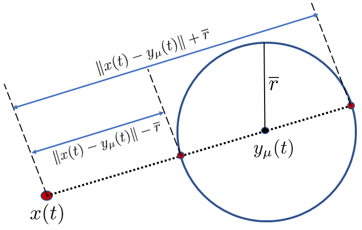
Figure 1: Illustration of simulation setting and measuring DTE for an agent at $x(t)$, facing an obstacle which is localized imperfectly in a circle of radius $\overline{r}$ and centered at $y_{\mu}(t)$.

With this, we assume the cost $c$ is distributed as a truncated Gaussian (Section III) with $c_{\mu}(\xi)=k_{1}\mathrm{e}^{-k_{2}d_{\mu}^{2}(\xi)}$ and $c_{\sigma}(\xi)=c_{\mu}(\overline{r})p^{\mathcal{N}}(\xi,\mathbf{I})$, where $d_{\mu}=\|x-y_{\mu}\|$ and $p^{\mathcal{N}}(\mu,\Sigma)$ is the pdf of a bi-variate Normal distribution with mean $\mu$ and covariance $\Sigma$ and $\mathbf{I}$ is the 2D identity matrix. We proceed to construct the uncertain cost outcomes according to Section III and then calculate $R^{\textup{cpt}},R^{v},R^{e}$ appropriately. We use the reference value $\rho=c_{\mu}(\overline{r})$, to denote the risk threshold.

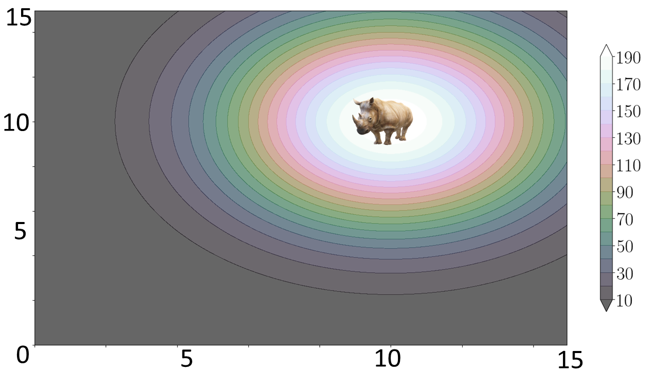
(a) Mean cost $c_{\mu}$ over $\mathcal{X}$

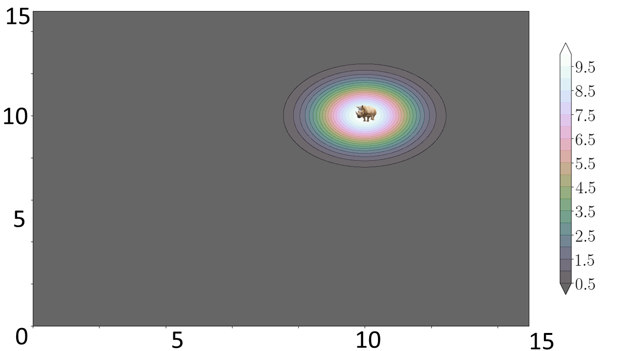
(b) Standard deviation $c_{\sigma}$ over $\mathcal{X}$

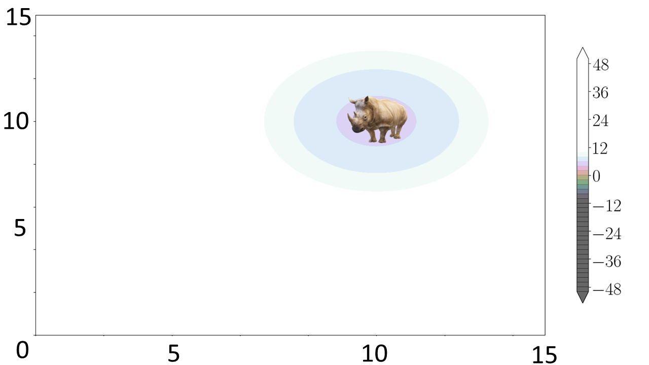
(c) Highly risk insensitive perception ($\gamma=0.45$ and $\rho=27$) with contour map depicting $\rho-R^{\textup{cpt}}$

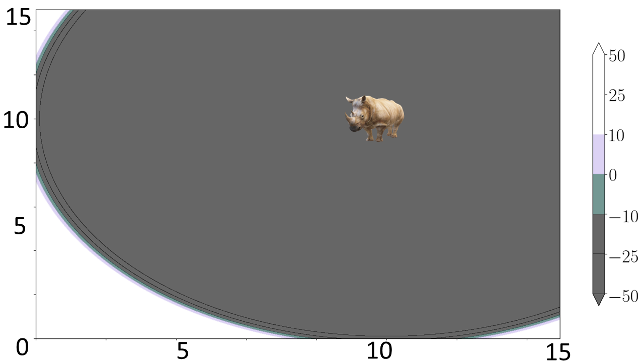
(d) Highly risk averse perception ($\lambda=100$ and $\rho=199$) with contour map depicting $\rho-R^{\textup{cpt}}$

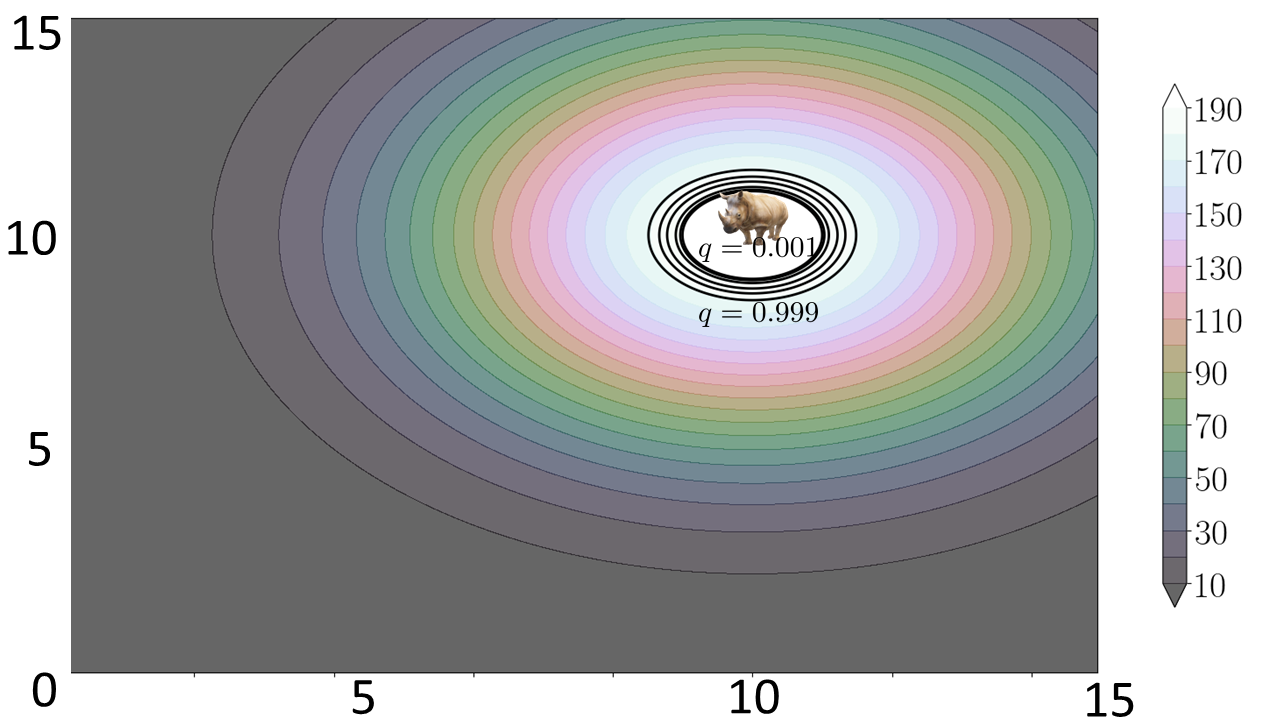
(e) Level sets of $R^{q}(\xi)=\rho$ by varying CVaR parameter $q\in\{0.001,0.1,0.4,0.8,0.95,0.999\}$

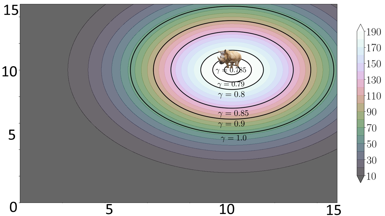
(f) Level sets of $R^{\textup{cpt}}(\xi)=\rho$ by varying risk sensitivity parameter $\gamma\in\{0.785,0.79,0.8,0.85,0.9,1.0\}$ with $\alpha=0.74,\beta=1,\lambda=3.0$

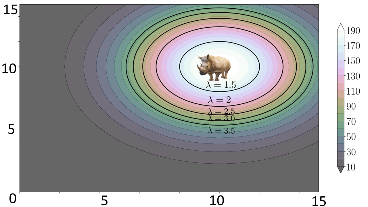
(g) Level sets of $R^{\textup{cpt}}(\xi)=\rho$ by varying risk aversion parameter $\lambda\in\{1.5,2.0,2.5,3.0,3.5\}$ with $\alpha=0.74,\beta=1,\gamma=0.95$

Figure 2: (a)-(b) Cost maps $c_{\mu}$ and $c_{\sigma}$ over the space $\mathcal{X}=[0,15]^{2}$ with obstacle’s mean position at $y_{\mu}=\{10,10\}$. (c)-(d) Illustration of versatility of CPT through depicting scalar field $\rho-R^{\textup{cpt}}$ in previous setting. (e)-(f) Change in perceived safety sets $\mathcal{X}_{\textup{safe}}$ by varying CPT parameters $\gamma$ and $\lambda$. (g) Change in perceived safety sets $\mathcal{X}_{\textup{safe}}$ by varying CVaR parameter $q$

Perceived safety visualization: Under the previous setting, we provide visualizations of the costs and perceived risks, shown in Fig. 2. Fig. 2(a) and 2(b) show the mean cost $c_{\mu}$ and standard deviation $c_{\sigma}$ respectively, across $\mathcal{X}=[0,15]^{2}$ with obstacle’s mean position at $y=(10,10)$ and $c_{\textup{min}}=1$ and $c_{\textup{max}}=200$. Versatility: CPT’s versatility is illustrated in Fig. 2(c) and Fig. 2(d) through contour maps of $h_{R}(\xi)=\rho-R^{\textup{cpt}}(x)$ across $\mathcal{X}$. Fig. 2(c) shows that despite risk threshold $\rho$ being very small ($\rho=27$) and close to $c_{\textup{min}}$, the entire space is perceived safe with positive $h$ values. In Fig. 2(d), we observe the opposite, where a very high risk threshold value ($\rho=199$), close to $c_{\textup{max}}$ still makes almost the entire $\mathcal{X}$ unsafe with negative $h_{R}(\xi)$ values. This illustrates the versatility of CPT as an RPM in accordance with Proposition 1.

Inclusiveness: This concept is illustrated in Fig. 2(e)–2(g). The black lines indicate the level sets of $R^{\textup{cpt}}=\rho$ and $R^{\textup{CV}}=\rho$ evaluated by varying their respective parameters. From Fig. 2(e) it is clear that variation in the level sets of CVaR is marginal compared to CPT (Fig. 2(f) and 2(g)). The level set $R^{\textup{ER}}(\xi)=\rho$ is shown in Fig. 2(e) as the inner most ellipse. We see that CPT is able to capture a more risk averse (larger) as well as more risk insensitive (smaller) perception than CVaR (and ER). This verifies the claims of Theorem 1 visually.

RPA-CBF controller: We consider a single agent with unicycle dynamics and a single obstacle whose dynamics evolve in the space $\mathcal{X}\subset^{2}$. We use the costs defined in the previous paragraph with $\overline{r}=0.5$ and $k_{1}=200,k_{2}=0.01$. The agent starts at $x(0)=(5,2)^{\top}$ (green dot) and its goal is $x^{*}=(10,10)^{\top}$ (motion up) while the obstacle moves from $(13,13)^{\top}$ (rhino in red ellipse) to $(2,3)^{\top}$ (motion down). If obstacle and vehicle follow along straight paths, a collision would occur and safety would be violated. To handle unicycle dynamics we use the projected point method to control a virtual point $p\in^{2}$, a distance $l$ along the direction of its heading. That is, $p=x+l\vec{d}$, where $\vec{d}$ is the direction vector corresponding to the agents heading $\phi$ and $x\in^{2}$ is the planar coordinates of the agent. With this we get the reverse transformation for the control inputs:

$$\begin{bmatrix}u_{1}\\ u_{2}\end{bmatrix}=\begin{bmatrix}\cos(\phi)&\sin(\phi)\\ \frac{-\sin(\phi)}{l}&\frac{\cos(\phi)}{l}\end{bmatrix}u.$$ (16)

Where $u_{1},u_{2}\in$ are the linear and angular velocity inputs of the unicycle model and $u\in^{2}$ is the optimized input generated from (7) considering the $p$ dynamics $\dot{p}=u$. We use a standard proportional controller for $k(x)$ with a constant $(0.6,0.6)$ We note that one can always appropriately tune the reference value $\rho$ by $l$ units to ensure safety w.r.t. $x$. The results of varying $\lambda$, $\gamma$ and $\kappa$ are shown in Fig. 3. For all the settings, the agent will collide with the obstacle (red ellipse) if it follows the nominal path (black line) from applying controls $k(x)$, thus making it unsafe. By using the controller $u$ from (7), the agent is able to swerve away from the obstacle in time and still manage to reach the goal. We see that from Fig. 3(d) - Fig. 3(f), the cbf $h_{R}$ remains positive throughout the execution, thus indicating that perceived safety is maintained irrespective of model and parameter choice. Next, we notice that by using CPT-CBF controller $u$ (Fig. 3(d) and Fig. 3(e)), the deviations from the nominal path correspondingly get more pronounced as the perceived risk increases (higher $\lambda$ and $\gamma$). Whereas, for CVaR-CBF this deviation (Fig. 3(f)) is comparatively minimal across its parameter spectrum. This is in accordance with our claims that CVaR is less inclusive (Theorem 1) and versatile (Proposition 1) than CPT, causing only minor changes in trajectories in comparison with CPT-based CBF controller.

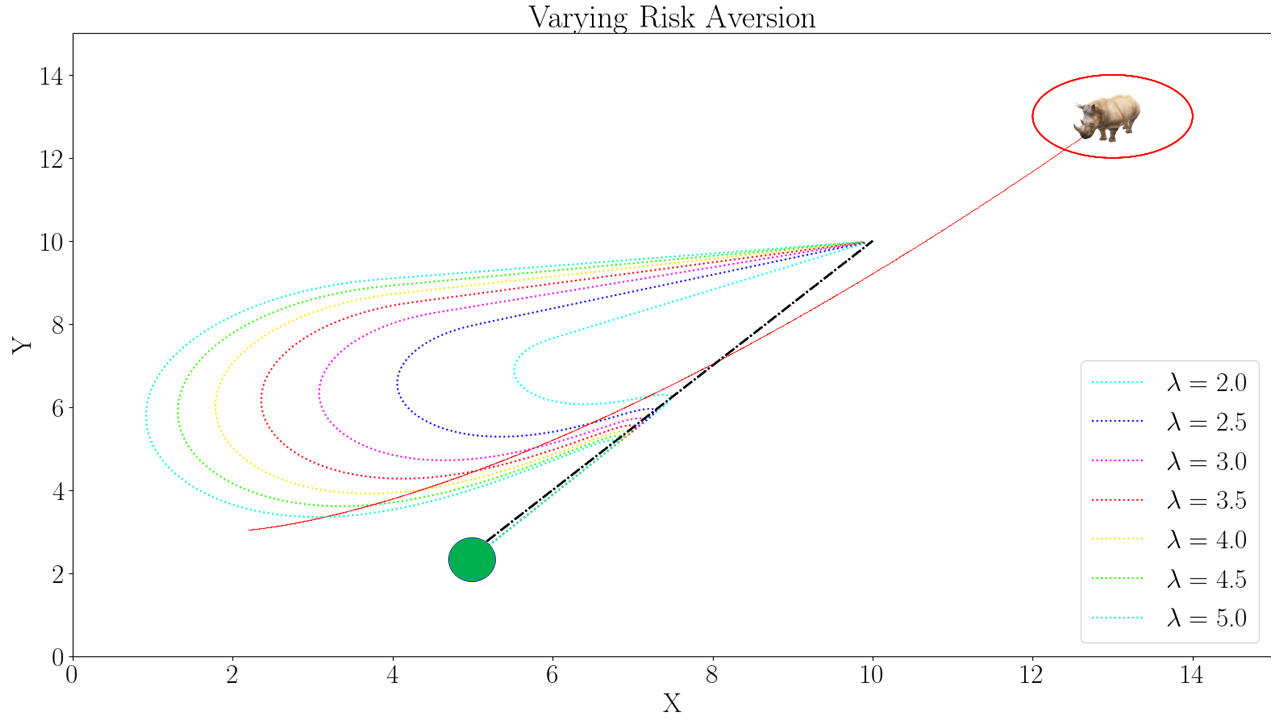
(a) Change in paths due to change in risk aversion $\lambda$ with $\gamma=0.88$

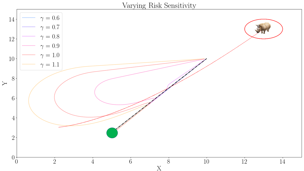
(b) Change in paths due to change in risk sensitivity $\gamma$ with $\lambda=2.25$

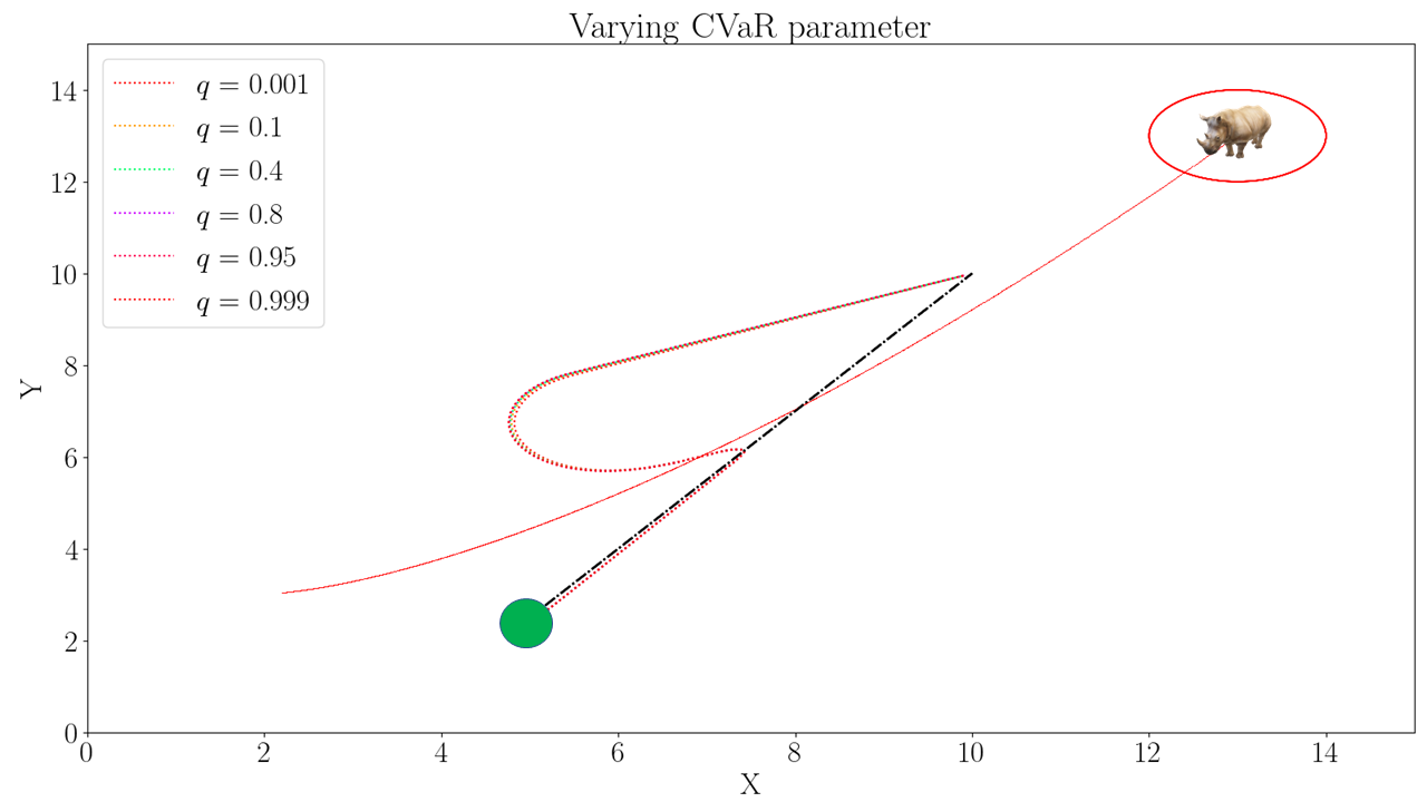
(c) Change in paths due to change in $\alpha$ with $\beta=1$

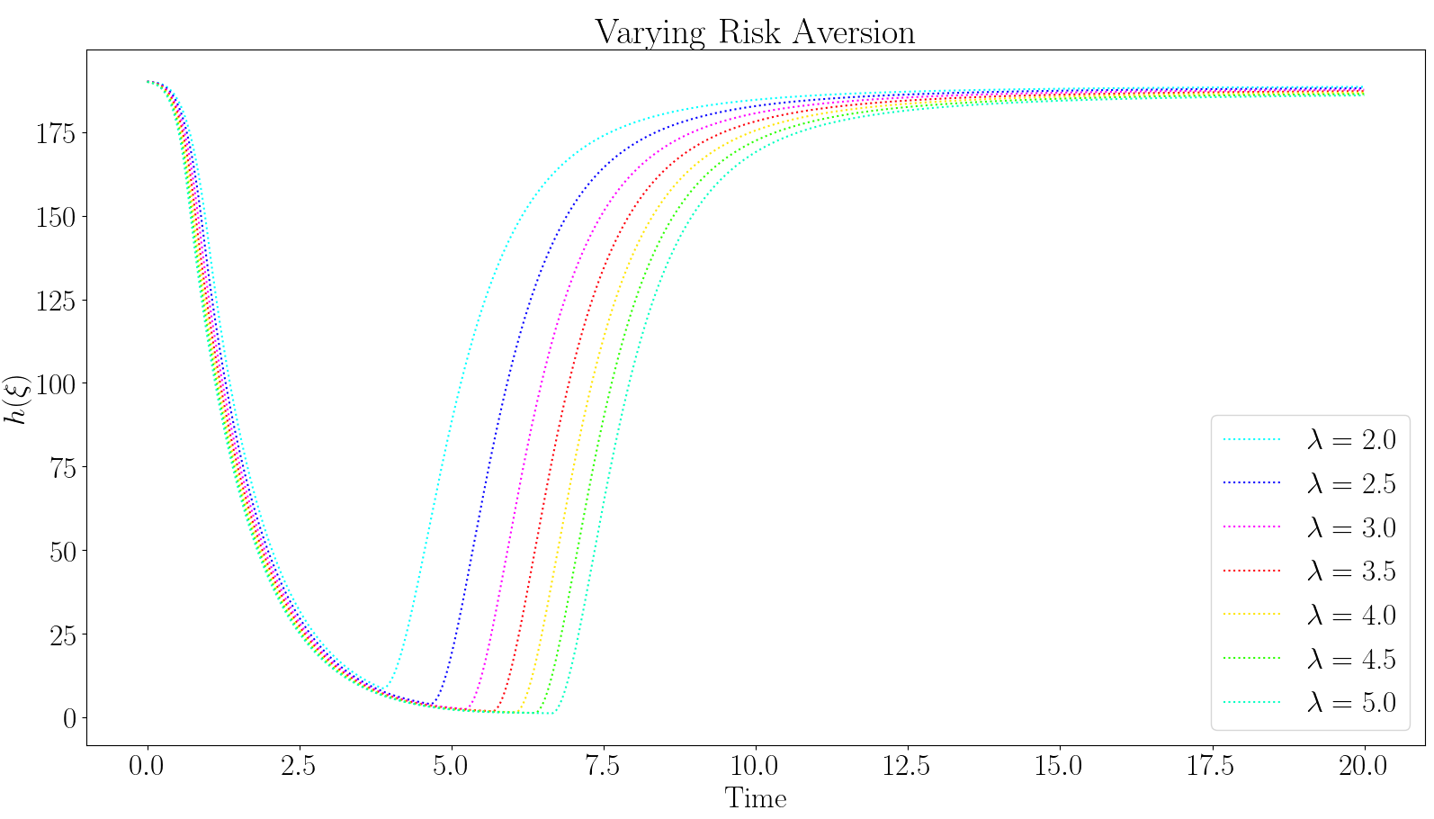
(d) Evolution of CBF function $h$ with varying $\lambda$

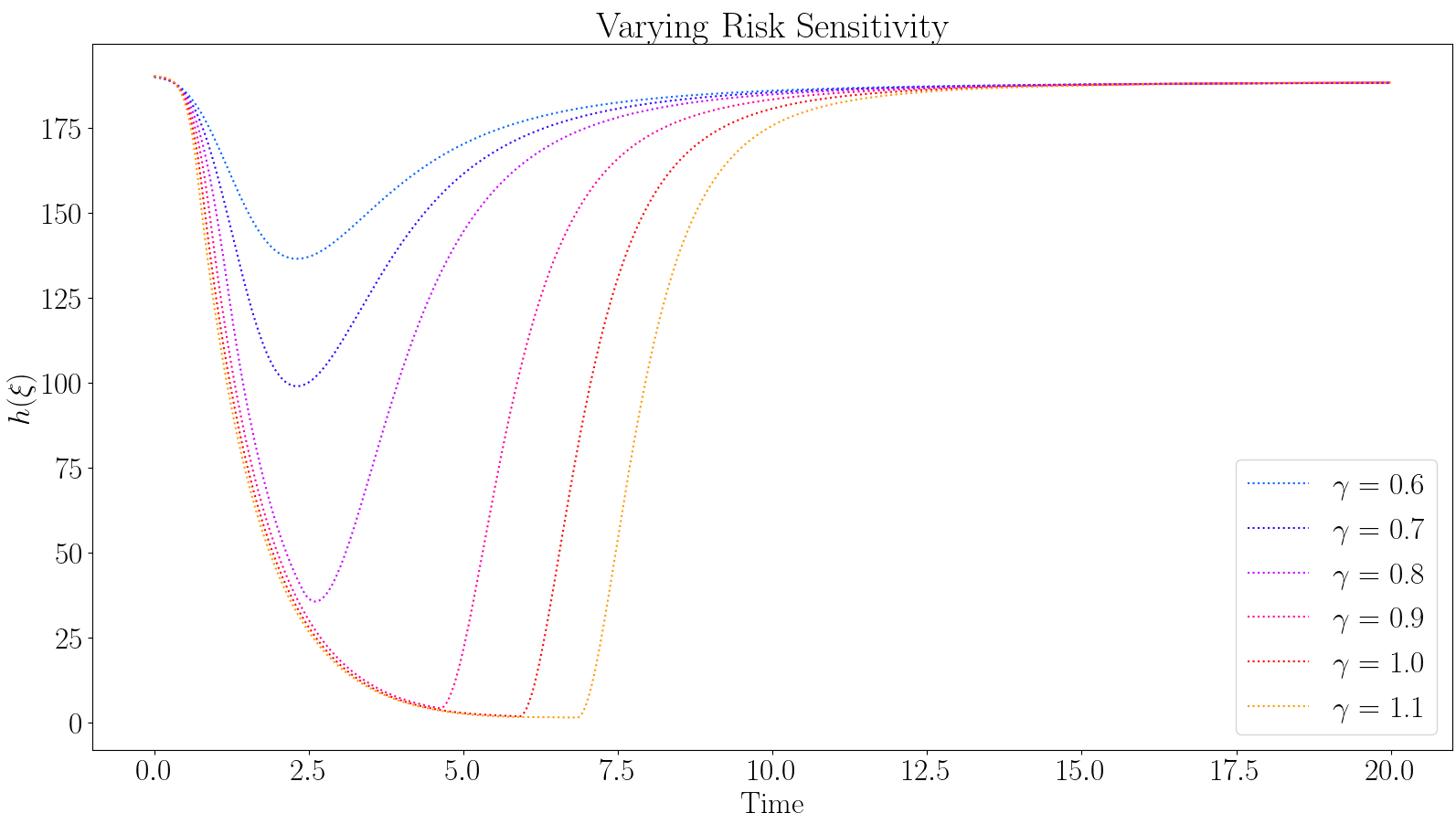
(e) Evolution of CBF function $h$ with varying $\gamma$

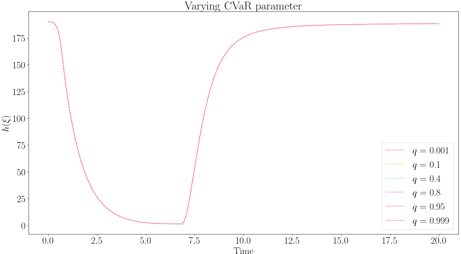
(f) Evolution of CBF function $h$ with varying $\kappa$ in CVaR

Figure 3: Path changes due to variation in risk aversion, risk sensitivity and CVaR parameter, with their corresponding CBF ($h$) evolution. The path of the obstacle (red) cross the nominal path of the agent (black) with the uncertainty circle indicated in red.

From (Fig. 3), we see that the agent is able to reach the goal while maintaining $h\geq 0$ throughout, implying that perceived safety is maintained according to Definition 1. Furthermore, as before, we see that CPT is able to generate a wider range of paths by tuning the risk aversion and risk sensitivity parameter than CVaR, thus capturing a greater variety of risk perception, which follows the theoretical arguments from Theorem 1 and Proposition 1. We also see that the agent also reaches the goal owing to the inherent stability properties of the nominal controller $k(x)$.

Next, we consider an environment where there are three moving obstacles present and a single agent. We use the composition approach proposed in [9] to construct the barrier function to handle multiple obstacles. In this approach, the worst case (closest) obstacle is dealt with first using the $\min$ operator on the barrier functions generated by the corresponding obstacles. Here, the agent has to go from $(-15,-15)$ to $(15,15)$, while the obstacles’ starting and goal points are respectively $(-17,0),(0,14),(10,-10)$ and $(17,0),(0,-14),(-10,10)$. Nominal controller $k(p)$ is generated with proportional constant $[1.6,1.6]$. The uncertainty radius is $\overline{r}=2.5$ and other cost constants are identical to the single agent setting. The results of varying the risk aversion $\lambda$, risk sensitivity $\gamma$ of CPT and $\kappa$ of CVaR are shown in Fig. 4.

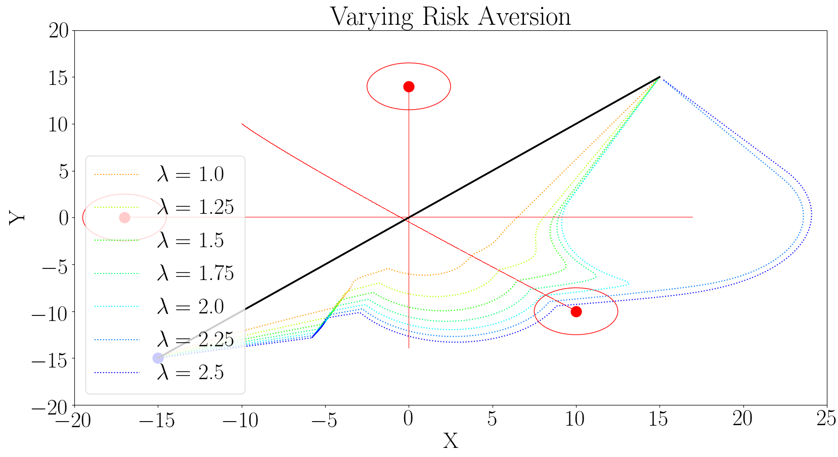
(a) Change in paths due to change in risk aversion $\lambda$ with $\gamma=0.88$

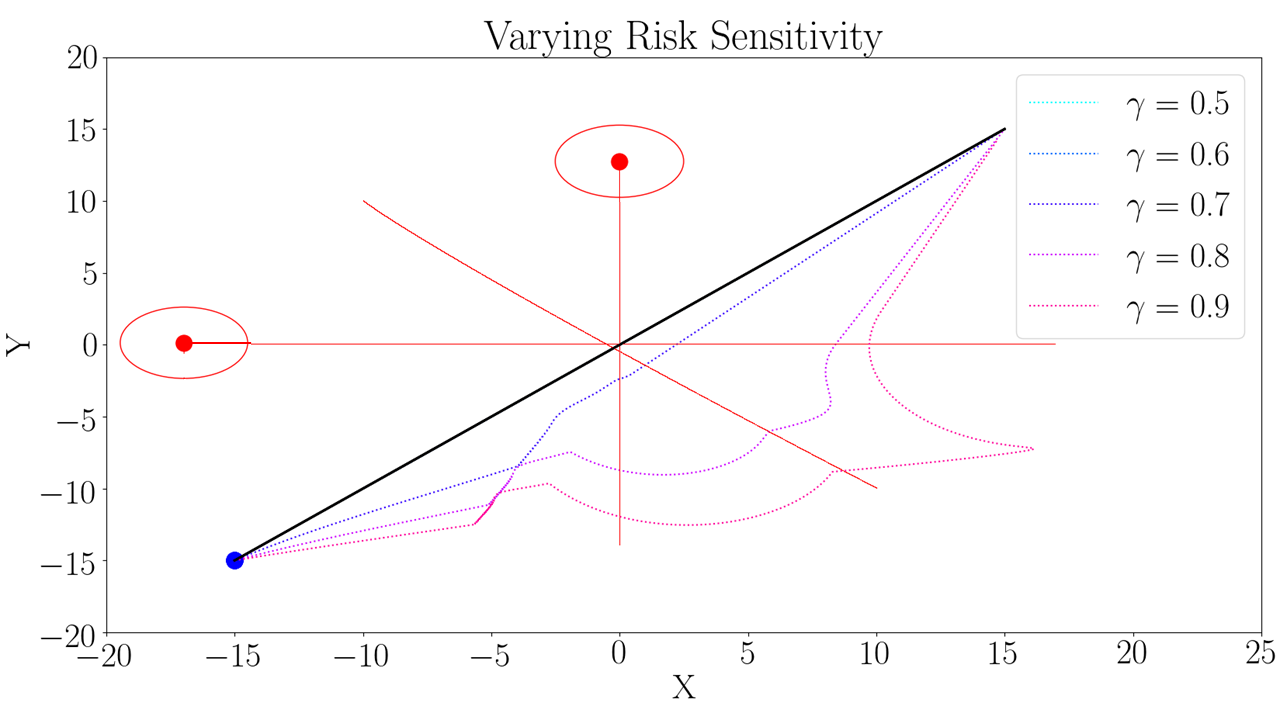
(b) Change in paths due to change in risk sensitivity $\gamma$ with $\lambda=2.25$

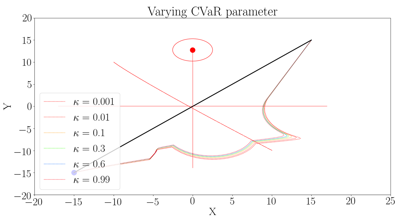
(c) Change in paths due to change in $\alpha$ with $\beta=1$

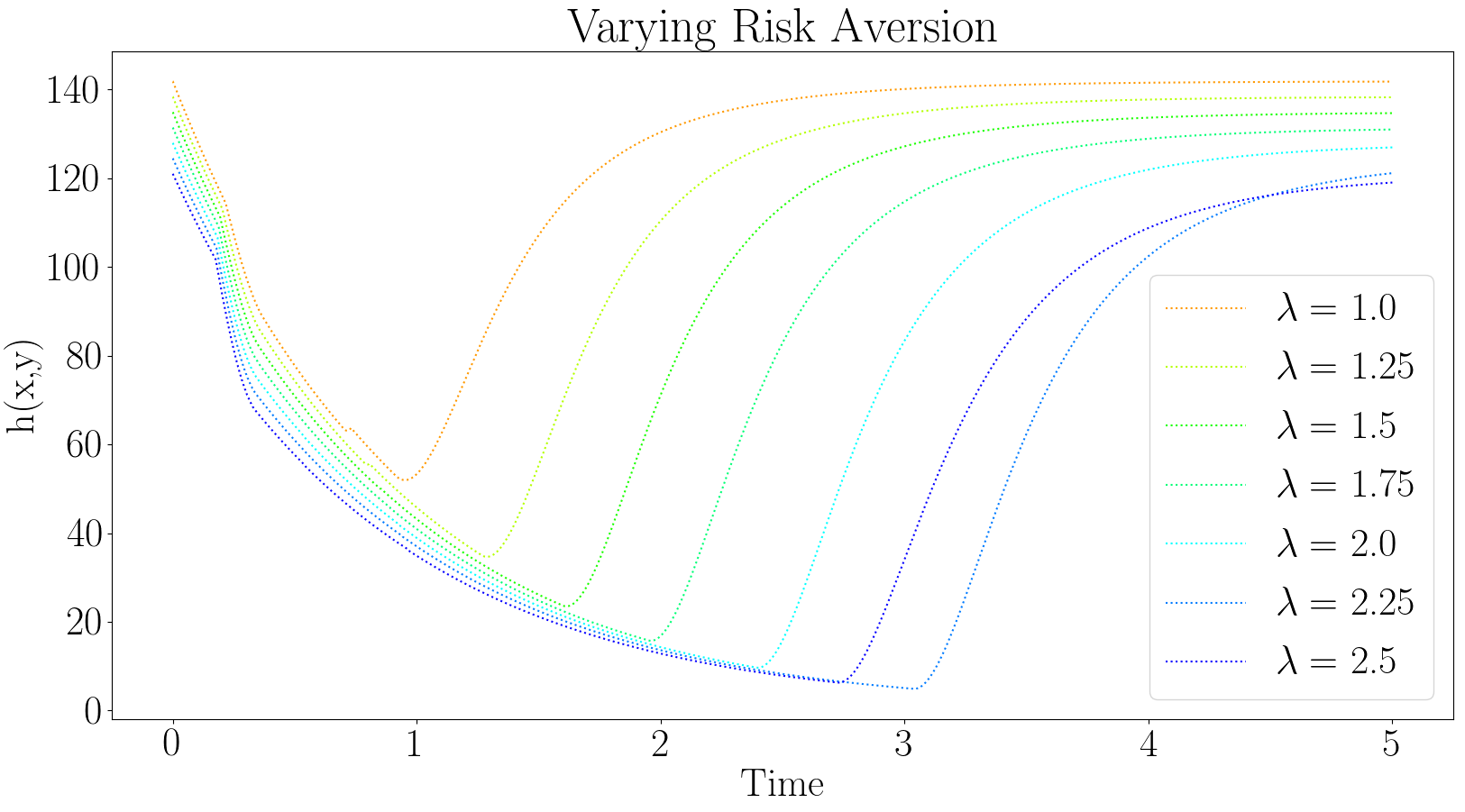
(d) Evolution of CBF function $h$ with varying $\lambda$

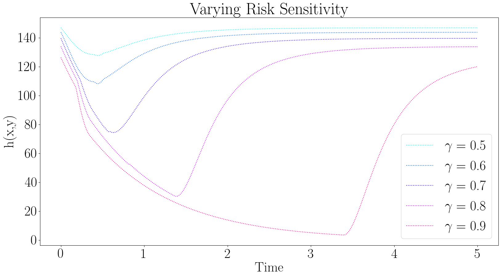
(e) Evolution of CBF function $h$ with varying $\gamma$

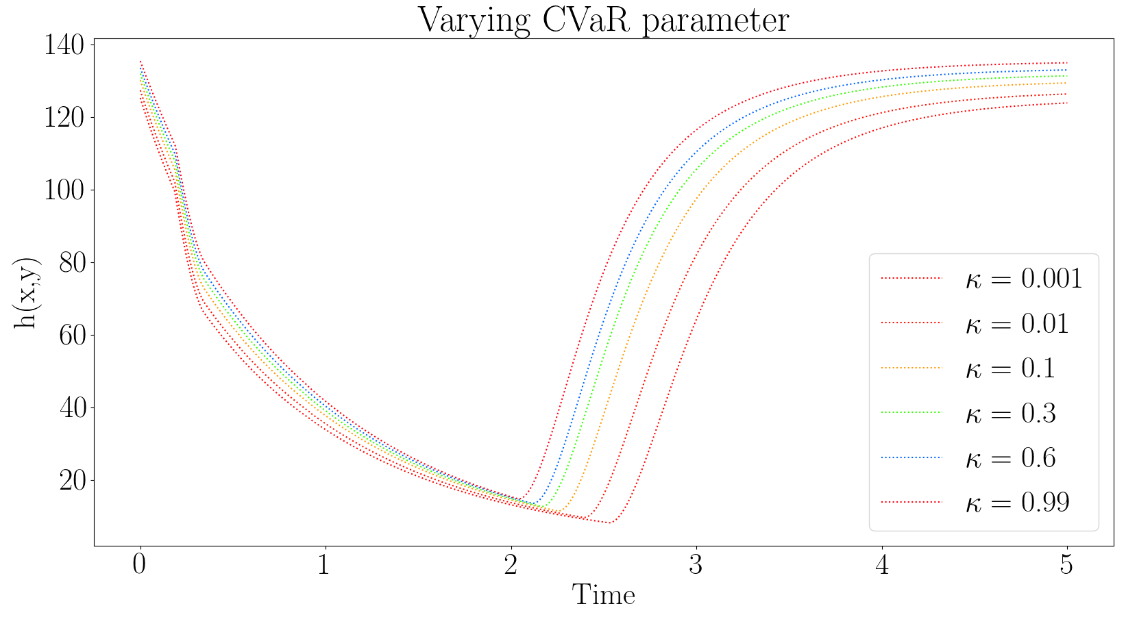
(f) Evolution of CBF function $h$ with varying $\kappa$ in CVaR

Figure 4: Path changes due to variation in risk aversion, risk sensitivity and CVaR parameter, with their corresponding CBF ($h$) evolution. The path of the obstacle (red) cross the nominal path of the agent (black) with the uncertainty circle indicated in red.

Similar to the previous case (Fig. 3), we see that the agent is able to reach the goal while maintaining $h\geq 0$ throughout, implying that perceived safety is maintained according to Definition 1. Furthermore, as before, we see that CPT is able to generate a wider range of paths by tuning the risk aversion and risk sensitivity parameter than CVaR, thus capturing a greater variety of risk perception, which follows the theoretical arguments from Theorem 1 and Proposition 1. We also see that in both the cases the agent also reaches the goal owing to the inherent stability properties of the nominal controller $k(x)$.

VI Conclusion and future work

In this work, we have proposed a novel integration of CPT (a non-rational decision making model) into a safety-critical control scheme, to generate risk-perception-aware (RPA) controls (according to a DM’s risk profile) in an environment embedded with uncertain costs. Thus, opening new avenues to incorporate behavioral decision theory into safety-critical controls. Future directions include the design of learning frameworks to determine the risk profile of an observed agent and handling unknown obstacle dynamics.

References

- [1] S. S. Stevens, “Neural events and the psychophysical law,” Science, vol. 170, no. 3962, pp. 1043–1050, 1970.
- [2] A. Tversky and D. Kahneman, “Advances in prospect theory: Cumulative representation of uncertainty,” Journal of Risk and Uncertainty, vol. 5, no. 4, pp. 297–323, 1992.
- [3] O. Khatib, Real-Time Obstacle Avoidance for Manipulators and Mobile Robots. Springer New York, 1990, pp. 396–404.
- [4] S. Prajna and A. Jadbabaie, “Safety Verification of Hybrid Systems using Barrier Certificates,” in Hybrid Systems: Computation and Control, 2004, pp. 477–492.
- [5] A. D. Ames, S. Coogan, M. Egerstedt, G. Notomista, K. Sreenath, and P. Tabuada, “Control barrier functions: Theory and applications,” in European Control Conference, 2019, pp. 3420–3431.
- [6] P. Ong and J. Cortés, “Universal formula for smooth safe stabilization,” in IEEE Int. Conf. on Decision and Control, Nice, France, Dec. 2019, pp. 2373–2378.
- [7] B. T. Lopez, J. J. E. Slotine, and J. P. How, “Robust adaptive control barrier functions: An adaptive and data-driven approach to safety,” IEEE Control Systems Letters, vol. 5, no. 3, pp. 1031–1036, 2021.
- [8] Y. Chen, H. Peng, and J. Grizzle, “Obstacle avoidance for low-speed autonomous vehicles with barrier function,” IEEE Transactions on Control Systems Technology, vol. 26, no. 1, pp. 194–206, 2018.
- [9] P. Glotfelter, J. Cortés, and M. Egerstedt, “Nonsmooth approach to controller synthesis for Boolean specifications,” IEEE Transactions on Automatic Control, vol. 66, no. 11, 2021, to appear.
- [10] S. Prajna, A. Jadbabaie, and G. J. Pappas, “A framework for worst-case and stochastic safety verification using barrier certificates,” IEEE Transactions on Automatic Control, vol. 52, no. 8, pp. 1415–1428, 2007.
- [11] A. Clark, “Control Barrier Functions for Complete and Incomplete Information Stochastic Systems,” in American Control Conference, 2019, pp. 2928–2935.
- [12] M. J. Khojasteh, V. Dhiman, M. Franceschetti, and N. Atanasov, “Probabilistic safety constraints for learned high relative degree system dynamics,” in Proceedings of Learning for Dynamics and Control, 2020, pp. 781–792.
- [13] S. Samuelson and I. Yang, “Safety-aware optimal control of stochastic systems using conditional value-at-risk,” in American Control Conference, 2018, pp. 6285–6290.
- [14] M. Ahmadi, X. Xiong, and A. D. Ames, “Risk-averse control via cvar barrier functions: Application to bipedal robot locomotion,” IEEE Control Systems Letters, vol. 6, no. 1, pp. 878–883, 2021.
- [15] A. Suresh and S. Martínez, “Planning under non-rational perception of uncertain spatial costs,” IEEE Robotics and Automation Letters, vol. 6, no. 2, pp. 4133–4140, 2021.
- [16] S. Gao, E. Frejinger, and M. Ben-Akiva, “Adaptive route choices in risky traffic networks: A prospect theory approach,” Transportation Research Part C: Emerging Technologies, vol. 18, no. 5, pp. 727–740, 2010.
- [17] A. R. Hota and S. Sundaram, “Game-Theoretic Protection against Networked sis Epidemics by Human Decision-Makers,” IFAC Papers Online, vol. 51, no. 34, pp. 145–150, 2019.
- [18] S. Dhami, The Foundations of Behavioral Economic Analysis. Oxford University press, 2016.
- [19] R. T. Rockafellar and S. Uryasev, “Optimization of conditional value-at-risk,” Journal of risk, vol. 2, no. 1, pp. 21–42, 2000.
- [20] D.Prelec, “The probability weighing function,” Econometrica, vol. 66, no. 3, pp. 497–527, 1998.