Ergodic Limits, Relaxations, and Geometric Properties of Random Walk Node Embeddings

Christy Lin, Daniel Sussman, and Prakash Ishwar Christy Lin is with the Division of Systems Engineering, College of Engineering, Boston University, 15 St Marys St, Boston, MA, 02215.
cy93lin@bu.edu Daniel Sussman is with the Department of Mathematics & Statistics, College of Arts and Sciences, Boston University, 111 Cummington Mall, Boston, MA, 02215. sussman@bu.edu Prakash Ishwar is with the Division of Systems Engineering and Department of Electrical & Computer Engineering, College of Engineering, Boston University, 8 St Marys St, Boston, MA, 02215. pi@bu.edu
Abstract

Random walk based node embedding algorithms learn vector representations of nodes by optimizing an objective function of node embedding vectors and skip-bigram statistics computed from random walks on the network. They have been applied to many supervised learning problems such as link prediction and node classification and have demonstrated state-of-the-art performance. Yet, their properties remain poorly understood. This paper studies properties of random walk based node embeddings in the unsupervised setting of discovering hidden block structure in the network, i.e., learning node representations whose cluster structure in Euclidean space reflects their adjacency structure within the network. We characterize the ergodic limits of the embedding objective, its generalization, and related convex relaxations to derive corresponding non-randomized versions of the node embedding objectives. We also characterize the optimal node embedding Grammians of the non-randomized objectives for the expected graph of a two-community Stochastic Block Model (SBM). We prove that the solution Grammian has rank 111 for a suitable nuclear norm relaxation of the non-randomized objective. Comprehensive experimental results on SBM random networks reveal that our non-randomized ergodic objectives yield node embeddings whose distribution is Gaussian-like, centered at the node embeddings of the expected network within each community, and concentrate in the linear degree-scaling regime as the number of nodes increases.

1 Introduction

Most statistical and computational tools originally developed for vector-valued data do not leverage the unique structured form of network data. Tools that exploit the graph-structure of network data could be custom-made for each network problem. A powerful alternative, however, is to develop a Euclidean-space embedding of a network that enables methods and tools developed for Euclidean-space data to effectively reason about various network properties.

Node embedding algorithms [1] aim to map nodes of a given graph into points in Euclidean space (i.e., vectors in dsuperscript𝑑\mathbb{R}^{d}) such that their relative positions capture their propensities for adjacency within the network. These embeddings

make it possible to apply to network data, tools and algorithms from multivariate statistics and machine learning that were developed for Euclidean-space data. For example, with suitable embeddings, node classification, community detection, and vertex nomination problems reduce, respectively, to standard classification, clustering, and ranking problems. Therefore, developing new node embedding algorithms, establishing the theoretical properties of these embeddings, and demonstrating how connectivity properties are reflected in the embedding space is fundamental to developing principled network inference procedures.

Random walk embeddings [2, 3, 4, 5] are a class of recently developed node embedding techniques which use random walks on graphs to capture notions of proximity between nodes. They may be viewed as network counterparts of techniques used for learning word embeddings [6, 7] in the field of natural language processing. In fact, by viewing samples of random walks in the network as sentences, with nodes playing the role of words, word embeddings can be directly applied to networks to yield node embeddings. Nodes which appear nearby within a sample of a random walk are analogous to words that appear nearby within a sentence. Word embeddings have been found to accurately capture the relationships between words and have been highly successful in several natural language processing tasks such as topic modeling, translation, and word analogy [8]. Random walk node embeddings too have been applied to a number of supervised and unsupervised learning problems such as link prediction, node classification and community detection and have demonstrated state-of-the-art performance [2, 3, 4, 5].

Unfortunately, despite excellent empirical performance in a number of supervised learning problems, random walk embeddings remain poorly understood. This is in stark contrast to the well-known spectral embeddings whose properties for the unsupervised learning problem of community detection have been extensively studied and characterized under a variety of statistical network models, specifically the Stochastic Block Model (SBM) and its generalizations [9, 10, 11, 12, 13, 14]. Attempts of theoretical analysis so far have focused on building connections between random walk embeddings algorithms and matrix factorization [15]. The properties of the resulting embedding vectors, however, still remain unexplored.

Contributions: This paper proposes a framework for random walk based node-embedding algorithms for graphs. This is based on learning node embeddings by optimizing objective functions involving skip-bigram statistics computed from random walks on a graph. This framework subsumes several existing algorithms as special cases and introduces extensions and techniques that simplify theoretical analysis. We establish ergodic limits of the proposed node-embeddings. We analyze Grammian re-parameterized convex relaxations and characterize the solution for the expected graph of a two-community SBM and the unconstrained solution for any graph. We prove that the solution of the expected graph of a two-community SBM has rank at most 222. We develop algorithms for computing solutions to our proposed embedding objectives for general graphs and conduct numerical experiments to understand the geometric structure of embedding vectors (community clustering and separation properties) for SBM random graphs. We also empirically study the concentration properties of node embeddings for SBM random graphs in the linear and logarithmic scaling regimes. We find empirically that the distribution of embeddings are Gaussian-like, centered at the node embeddings of the expected graph within each community, and that they concentrate in the linear degree scaling regime as the number of nodes increases.

Paper organization: Section 2 overviews recent work on random walk embeddings, sets up basic notation, and provides background on SBMs. Section 3 describes our proposed theoretical framework, results on ergodic limits (Section 3.1), various relaxations (Section 3.3), and the characterization of the solution for the expected graph of a two-community SBM (Section 3.4). Section 4 describes the setting of all our experiments in full detail. The geometric and concentration properties of the distribution of embedding vectors of our proposed algorithms under 2-community SBM are presented and discussed in Section 5. Concluding remarks appear in Section 6.

Notation: In this work we consider graphs that are undirected and simple with a node set 𝒱=[n]:={1,2,,n}𝒱delimited-[]𝑛assign12𝑛\mathcal{V}=[n]:=\{1,2,\dotsc,n\} and an edge set {{i,j}:i,jV,ij}conditional-set𝑖𝑗formulae-sequence𝑖𝑗𝑉𝑖𝑗\mathcal{E}\subset\{\{i,j\}:i,j\in V,i\neq j\}. The edges may be possibly weighted. We denote such a graph by 𝒢=(𝒱,)𝒢𝒱\mathcal{G}=(\mathcal{V},\mathcal{E}) and its adjacency matrix by A{0,1}n×n𝐴superscript01𝑛𝑛A\in\{0,1\}^{n\times n}, where Aij=0subscript𝐴𝑖𝑗0A_{ij}=0 if, and only if, {i,j}𝑖𝑗\{i,j\}\in\mathcal{E}.

We denote the set of all real numbers by \mathbb{R}, the set of all natural numbers by \mathbb{N}, the set of all n×n𝑛𝑛n\times n real symmetric matrices by 𝕊nsuperscript𝕊𝑛\mathbb{S}^{n}, the set of all real, symmetric, and positive semidefinite matrices by 𝕊+nsubscriptsuperscript𝕊𝑛\mathbb{S}^{n}_{+}, and the natural logistic-loss function by σ(t):=ln(1+et),tformulae-sequenceassign𝜎𝑡1superscript𝑒𝑡𝑡\sigma(t)\vcentcolon=\ln(1+e^{-t}),t\in\mathbb{R}. Matrix transpose is denoted by .

2 Background and related work

In this section we overview recent work on random walk node embeddings with a focus on the unsupervised algorithm VEC. We also summarize key aspects of the Stochastic Block Model (SBM) used in our experiments.

2.1 Random walk node embedding algorithms

A random walk node embedding algorithm typically consists of three steps: 1) Generating multiple random walks over the graph via Markov chains with the set of nodes as the state space, specified probability transition matrices at each step, and specified initial distributions. 2) Computing various statistics from the sample paths of the random walks. 3) Generating embeddings by optimizing a function that only involves the computed statistics and node embedding variables of the input graph.

Among the random walk node embedding algorithms, [2, 4, 16] make use of node embeddings within the context of supervised learning problems such as node attribute prediction and link prediction and accordingly design probability transition matrices that depend on the supervised labels. In contrast, the VEC algorithm [5] focuses on the unsupervised community detection problem [17]. The unsupervised setting of [5] is ideal for studying random walk node embeddings that capture pure network connectivity properties unsullied by node labels. We therefore select VEC as our prototypical algorithm for analysis and introduce it in detail in the next subsection.

While our focus is on unsupervised setting, the general Markov-Chain based framework we develop can be used to analyze the supervised setting as well through transition matrices that are label dependent.

In addition to the node embedding algorithms discussed above, the use of a random walks and their steady-state-distributions for graph clustering has been studied in [18] and [19]. Subsequent work [20] further proposed to exploit multi-step transition probabilities between nodes for clustering.

In terms of theoretical results, [21] have analyzed the stationary distribution of second-order random walks in [4] for specific types of networks. We provide a complete characterization of the ergodic limits for general random walk node embedding objectives in Section 3. For the task of community detection, [22] have provided large-sample error bounds for consistent community recovery from the perspective of matrix factorization. Their setting is a special, unconstrained case of our general problem stated in Definition 6 of Section 3.3.

2.2 VEC: unsupervised random walk node embedding

VEC learns a low-dimensional vector representation for each node of a graph such that the local neighborhood structures of the graph are encoded within the Euclidean geometry of node vectors. Specifically, the inner product between the embedding vectors of node pairs encode their propensity to appear nearby in random walks on the graph.

VEC generates r𝑟r random walks on 𝒢𝒢\mathcal{G} of fixed length \ell starting from each node. We let {Xs(m,p)}s=1,p=1,,rformulae-sequencesuperscriptsubscriptsuperscriptsubscript𝑋𝑠𝑚𝑝𝑠1𝑝1𝑟\{X_{s}^{(m,p)}\}_{s=1}^{\ell},p=1,\ldots,r, denote the p𝑝p-th random walk starting from node m𝑚m. All random walks follow the “natural” transition matrix W𝑊W where the next node is chosen from the immediate neighbors of the current node with probability proportional to the edge weight between them.

VEC learns node embedding using the negative-sampling framework of noise-contrastive estmation [6]. The statistics used for learning node embeddings are based on two multisets of node pairs that are computed from the sample paths of the random walks as follows. The positive multiset 𝒟+subscript𝒟\mathcal{D}_{+} consists of all node pairs (Xs(m,p),Xs(m,p))subscriptsuperscript𝑋𝑚𝑝𝑠subscriptsuperscript𝑋𝑚𝑝superscript𝑠(X^{(m,p)}_{s},X^{(m,p)}_{s^{\prime}}), including repetitions, that occur within w𝑤w steps of each other, i.e., |ss|w𝑠superscript𝑠𝑤|s-s^{\prime}|\leq w, in all the generated sample paths. Such node pairs are called w𝑤w-skip bigrams in Natural Language Processing with words viewed as nodes and sentences as sample paths of random walks. The algorithm parameter w𝑤w controls the size of the local neighborhood of a node in the given graph. The negative multiset 𝒟subscript𝒟\mathcal{D}_{-} is constructed as follows. For each node pair (i,j)𝑖𝑗(i,j) in 𝒟+subscript𝒟\mathcal{D}_{+}, we append k𝑘k node pairs (i,j1),,(i,jk)𝑖subscript𝑗1𝑖subscript𝑗𝑘(i,j_{1}),\ldots,(i,j_{k}) to 𝒟subscript𝒟\mathcal{D}_{-}, where the k𝑘k nodes j1,,jksubscript𝑗1subscript𝑗𝑘j_{1},\ldots,j_{k} are drawn in an IID manner from all the nodes according to the empirical unigram node distribution computed from all the sample paths. Let nij+superscriptsubscript𝑛𝑖𝑗n_{ij}^{+} and nijsuperscriptsubscript𝑛𝑖𝑗n_{ij}^{-} denote the number of (i,j)𝑖𝑗(i,j) pairs, counting repetitions, in 𝒟+subscript𝒟\mathcal{D}_{+} and 𝒟subscript𝒟\mathcal{D}_{-} respectively.

VEC finds the embedding vector 𝒖idsubscript𝒖𝑖superscript𝑑\bm{u}_{i}\in\mathbb{R}^{d} for each node i𝑖i by solving the following minimization problem:

Definition 1 (VEC optimization problem).
argmin{𝐮id,i𝒱}(i,j)𝒱2[nij+σ(𝐮i𝐮j)+nijσ(𝐮i𝐮j)]formulae-sequencesubscript𝐮𝑖superscript𝑑𝑖𝒱subscript𝑖𝑗superscript𝒱2delimited-[]superscriptsubscript𝑛𝑖𝑗𝜎superscriptsubscript𝐮𝑖topsubscript𝐮𝑗superscriptsubscript𝑛𝑖𝑗𝜎superscriptsubscript𝐮𝑖topsubscript𝐮𝑗\displaystyle\underset{\{\mathbf{u}_{i}\in\mathbb{R}^{d},i\in\mathcal{V}\}}{\arg\min}\sum_{(i,j)\in\mathcal{V}^{2}}\left[n_{ij}^{+}\;\sigma(\mathbf{u}_{i}^{\top}\mathbf{u}_{j})+n_{ij}^{-}\;\sigma(-\mathbf{u}_{i}^{\top}\mathbf{u}_{j})\right] (1)

One approach to solve Eq. (1) is via stochastic gradient descent (SGD) [23, 24]. This approach is followed in [6] and implemented in Python gensim package. Besides its conceptual simplicity, SGD can be parallelized and nicely scaled to large datasets [25]. The per-iteration computational complexity of the SGD algorithm used to solve Eq. (1) is O(d)𝑂𝑑O(d), i.e., linear in the emebdding dimension. The number of iterations is O(rwk)𝑂𝑟𝑤𝑘O(r\ell wk).

2.3 Stochastic Block Model

The Stochastic Block Model (SBM) [26, 27, 28] is a canonical generative probabilistic model for random graphs that reflects block (community) structures among the nodes wherein nodes within the same block have the same tendencies for connecting to all other nodes. Free of node or edge labels, it serves as a clean platform for generating graphs to empirically study and compare the properties of various node embedding algorithms and conduct a theoretical analysis. For example, SBM has helped in understanding the behavior of spectral embeddings [12].

For any given K𝐾K\in\mathbb{N}, a K𝐾K-block SBM is parameterized by the latent block membership labels y1,,yn[K]subscript𝑦1subscript𝑦𝑛delimited-[]𝐾y_{1},\dotsc,y_{n}\in[K], and the edge probability matrix, a symmetric matrix B[0,1]K×K𝐵superscript01𝐾𝐾B\in[0,1]^{K\times K}. The latent labels {yi}subscript𝑦𝑖\{y_{i}\} partition the nodes into communities indexed by each k[K]𝑘delimited-[]𝐾k\in[K]. We note that there are versions of SBM in which the yisubscript𝑦𝑖y_{i}’s are treated as random. This, however, poses minor additional difficulties. To ease the subsequent discussion, unless noted otherwise, the yisubscript𝑦𝑖y_{i}’s will always be viewed as fixed deterministic unknowns throughout this work. For a node in block k1subscript𝑘1k_{1} and a different node in block k2subscript𝑘2k_{2} (where k2subscript𝑘2k_{2} may equal k1subscript𝑘1k_{1}), the probability that an edge is present between the two nodes is Bk1k2subscript𝐵subscript𝑘1subscript𝑘2B_{k_{1}k_{2}}, and all edges appear independently. We use this model for generating graphs in all our experiments.

The goal of any community detection algorithm is to learn the latent communities of nodes purely from the graph structure. Thus community detection is an unsupervised learning problem which aims to uncover the underlying block structure. A series of work [29, 30, 31, 32, 33, 34] characterizes the information-theoretic limits of community detection in SBMs in different degree-scaling regimes. Some of our experiments are designed to operate with respect to these information-theoretic limits.

3 Analytical framework and results

There are three distinct challenges which complicate the analysis of VEC embedding vectors and their relationship to the latent graph community structure. First, the objective function Eq. (1) is nonlinear due to the logistic loss function. Second, even though the function σ(t)𝜎𝑡\sigma(t) is strictly convex, the overall objective is not convex with respect to the node embedding vectors. Finally, the objective function is itself random, partly due to intrinsic randomness in network connectivity, but also due to algorithmic randomness from the random walks and the Stochastic Gradient Descent algorithm.

VECGramVECequivalentPMIno constraintsErgoVEClimlsubscript𝑙\lim_{l\to\infty}GramErgoVEClimlsubscript𝑙\lim_{l\to\infty}equivalentErgoPMIno constraintslimlsubscript𝑙\lim_{l\to\infty}NucGramErgoVECrank\to\|\cdot\|_{*}Projected ErgoPMIrank-d𝑑dp.s.d. proj.
Figure 1: Relationships between analysis strategies.

To tackle these challenges, in this section we introduce and develop techniques, generalized formulations, and their extensions which are more amenable to theoretical analysis. We leverage three distinct strategies whose inter-relationships are succinctly depicted in Fig. 1. These are:

  • (1)

    ErgoVEC: Ergodic limits of random walks (limsubscript\lim_{\ell\rightarrow\infty}). We begin by noting that the sampled coefficients, nij+superscriptsubscript𝑛𝑖𝑗n_{ij}^{+}’s and nijsuperscriptsubscript𝑛𝑖𝑗n_{ij}^{-}’s in Eq. (1), inherit the randomness of the random walks and depend on a number of algorithm parameters that are described in Sec. 2.2. Previous empirical results [5] demonstrate that the parameters such as the number of random walks r𝑟r and their length \ell do not substantially impact performance. Motivated by this observation, as a first step, in Sec. 3.1, we eliminate algorithmic randomness by taking the ergodic limits (\ell\rightarrow\infty) of the coefficients. This gives rise to a more principled formulation, which we call ErgoVEC, that removes dependence on sampled random walks and parameters r𝑟r and \ell.

  • (2)

    GramErgoVEC and PMI: reparameterize, unconstrain and project. Like VEC, ErgoVEC is a nonconvex optimization problem since the objective is a noconvex function of the embedding vectors 𝐮isubscript𝐮𝑖\mathbf{u}_{i}. We leverage a re-parametrization trick which is similar in spirit to that used in [35] to arrive at an equivalent problem, named GramErgoVEC, that has a convex objective function with respect to new matrix variables and additional constraints. GramErgoVEC has a convex objective, but is still a nonconvex optimization problem due to the rank constraint. In order to gain insight into the structure of the solution, we characterize the solution to GramErgoVEC without any constraints and then project the unconstrained solution onto the constraint set. It turns out that the solution to the unconstrained GramErgoVEC objective is directly related to the so-called Pointwise Mutual Information (PMI) matrix [36]. We study GramErgoVEC and PMI in Sec. 3.3

  • (3)

    NucGramErgoVEC: reparameterize and convexify. Another strategy to convexify GramErgoVEC is to replace the non-convex rank constraint by a convex nuclear norm constraint. We term the resulting optimization problem NucGramErgoVEC and study its properties in the later part of Sec. 3.3

In the rest of this section, we will formally study and establish important theoretical properties of these alternative formulations and their inter-relationships.

3.1 Ergodic limits

As described in Sec. 2.2, nij+superscriptsubscript𝑛𝑖𝑗n_{ij}^{+} and nijsuperscriptsubscript𝑛𝑖𝑗n_{ij}^{-} are the number of the (i,j)𝑖𝑗(i,j) node pairs in the positive and negative multisets, 𝒟+subscript𝒟\mathcal{D}_{+} and 𝒟subscript𝒟\mathcal{D}_{-}, respectively. These depend on 555 algorithm parameters: r𝑟r (number of random walks per node), \ell (length of each walk), w𝑤w (context window size) and k𝑘k (number of negative w𝑤w-skip bigrams per positive w𝑤w-skip bigram). Specifically, nij+superscriptsubscript𝑛𝑖𝑗n_{ij}^{+}, as a w𝑤w-skip bigram count over r𝑟r IID sets of n𝑛n random walks, increases proportionally with r𝑟r and n𝑛n and roughly proportionately with \ell, for large \ell, since the number of segments of w𝑤w consecutive steps in a length-\ell walk equals (lw+1)𝑙𝑤1(l-w+1). They also increase as w𝑤w increases however their distribution can change substantially with w𝑤w. As for the negative multiset, note that |𝒟|=k|𝒟+|subscript𝒟𝑘subscript𝒟|\mathcal{D}_{-}|=k|\mathcal{D}_{+}|, so nijsuperscriptsubscript𝑛𝑖𝑗n_{ij}^{-} increases proportional to k,r𝑘𝑟k,r, and \ell. Among these parameters, the results in [5] show that r𝑟r and \ell have little effect on the final performance of VEC, while w𝑤w plays a more important role.

Besides their dependence on the algorithm parameters, nij+superscriptsubscript𝑛𝑖𝑗n_{ij}^{+}’s and nijsuperscriptsubscript𝑛𝑖𝑗n_{ij}^{-}’s inherit the randomness intrinsic to the random walks. Additionally, the number of negative (i,j)𝑖𝑗(i,j) pairs nijsuperscriptsubscript𝑛𝑖𝑗n_{ij}^{-} also inherit randomness from the categorical sampling of appended nodes j1,,jksubscript𝑗1subscript𝑗𝑘j_{1},\dots,j_{k} in the negative pairs. In order to gain an algorithmic-randomness-free understanding of network properties captured by nij+superscriptsubscript𝑛𝑖𝑗n_{ij}^{+} and nijsuperscriptsubscript𝑛𝑖𝑗n_{ij}^{-}, we study their ergodic limits.

Definition 2 (Ergodic limits of nij+superscriptsubscript𝑛𝑖𝑗n_{ij}^{+} and nijsuperscriptsubscript𝑛𝑖𝑗n_{ij}^{-}).

Let nij+superscriptsubscript𝑛𝑖𝑗n_{ij}^{+} and nijsuperscriptsubscript𝑛𝑖𝑗n_{ij}^{-} be defined as above. The (normalized) ergodic limits of nij+superscriptsubscript𝑛𝑖𝑗n_{ij}^{+} and nijsuperscriptsubscript𝑛𝑖𝑗n_{ij}^{-} are defined as

n¯ij+:=assignsuperscriptsubscript¯𝑛𝑖𝑗absent\displaystyle\bar{n}_{ij}^{+}:={} 1rnlimnij+,1𝑟𝑛subscriptsuperscriptsubscript𝑛𝑖𝑗\displaystyle\frac{1}{rn}\lim\limits_{\ell\rightarrow\infty}\frac{n_{ij}^{+}}{\ell}, (2)
n¯ij:=assignsuperscriptsubscript¯𝑛𝑖𝑗absent\displaystyle\bar{n}_{ij}^{-}:={} 1rnlimnij,1𝑟𝑛subscriptsuperscriptsubscript𝑛𝑖𝑗\displaystyle\frac{1}{rn}\lim\limits_{\ell\rightarrow\infty}\frac{n_{ij}^{-}}{\ell}, (3)

whenever these limits exist in the almost sure sense.

The Ergodic limits in Definition 2 provide, for a given graph, a deterministic version of nij+superscriptsubscript𝑛𝑖𝑗n_{ij}^{+} and nijsuperscriptsubscript𝑛𝑖𝑗n_{ij}^{-}, normalized by the cumulative length of all random walks. We note that letting \ell go to infinity may seem like incorporating global information about the entire graph instead of the more useful local connectivity patterns, but this is not the case. Regardless of the value of \ell, 𝒟+subscript𝒟\mathcal{D}_{+} only contains pairs of nodes which appear within w𝑤w steps from each other. Therefore, the positive pairs sampled still reflect local information.

In VEC we launch r𝑟r random walks starting deterministically from each node which yields a total of rn𝑟𝑛rn random walks. Dividing the w𝑤w-skip bigram counts by rn𝑟𝑛rn averages them across all random walks. The averaged counts can be loosely viewed as arising from a single random walk with a uniform initial distribution over nodes, i.e., with probability 1/n1𝑛1/n for each node. If the Markov Chain underlying the random walk is ergodic, as \ell tends to infinity, the nij+superscriptsubscript𝑛𝑖𝑗n_{ij}^{+}’s and nijsuperscriptsubscript𝑛𝑖𝑗n_{ij}^{-}’s, suitably normalized, will converge to their respective expected values under the sampling distribution of random walks. This intuition is formalized in Theorem 1 below. The theorem encompasses disconnected graphs that consist of several connected components that are often encountered in practice. In such cases, the random walks can be launched within and confined to each connected component. The theorem also covers the case where edges in the graph have real-valued (non-binary) nonnegative weights. The theorem provides explict closed-form expressions for the ergodic limits n¯ij+superscriptsubscript¯𝑛𝑖𝑗\bar{n}_{ij}^{+} and n¯ijsuperscriptsubscript¯𝑛𝑖𝑗\bar{n}_{ij}^{-}.

Theorem 1 (Ergodic limits of nij+superscriptsubscript𝑛𝑖𝑗n_{ij}^{+} and nijsuperscriptsubscript𝑛𝑖𝑗n_{ij}^{-}).

Let 𝒢𝒢\mathcal{G} be a weighted graph with connected components {𝒢t}t=1msuperscriptsubscriptsubscript𝒢𝑡𝑡1𝑚\{\mathcal{G}_{t}\}_{t=1}^{m}, where for each t𝑡t, 𝒢tsubscript𝒢𝑡\mathcal{G}_{t} has ntsubscript𝑛𝑡n_{t} nodes and a nonnegative weighted adjacency matrix Atsubscript𝐴𝑡A_{t}. Let the VEC algorithm be executed on 𝒢𝒢\mathcal{G} with parameters w𝑤w and k𝑘k and transition matrix Wt:=Dt1Atassignsubscript𝑊𝑡superscriptsubscript𝐷𝑡1subscript𝐴𝑡W_{t}\vcentcolon={}D_{t}^{-1}A_{t} in component t𝑡t, where Dtsubscript𝐷𝑡D_{t} is a diagonal matrix with i𝑖ith diagonal element Dt,ii=jAt,ij=:diD_{t,ii}=\sum_{j}A_{t,ij}=:d_{i}, i.e., the degree of node i𝑖i. Then the ergodic limits n¯ij+superscriptsubscript¯𝑛𝑖𝑗\bar{n}_{ij}^{+}’s and n¯ijsuperscriptsubscript¯𝑛𝑖𝑗\bar{n}_{ij}^{-}’s in Definition 2 exist and are given by

n¯ij+=superscriptsubscript¯𝑛𝑖𝑗absent\displaystyle\bar{n}_{ij}^{+}={} {πiv=1w(Wtv)ij,if i,j𝒢t;0otherwise.,casessubscript𝜋𝑖superscriptsubscript𝑣1𝑤subscriptsuperscriptsubscript𝑊𝑡𝑣𝑖𝑗if 𝑖𝑗subscript𝒢𝑡0otherwise\displaystyle\begin{cases}\pi_{i}\sum_{v=1}^{w}(W_{t}^{v})_{ij},&\text{if }i,j\in\mathcal{G}_{t};\\ 0&\text{otherwise}.\end{cases}, (4)
n¯ij=superscriptsubscript¯𝑛𝑖𝑗absent\displaystyle\bar{n}_{ij}^{-}={} kwπiπj,𝑘𝑤subscript𝜋𝑖subscript𝜋𝑗\displaystyle kw\pi_{i}\pi_{j}, (5)

where π𝜋\mathbf{\pi} is a stationary distribution of the random walk with πi=nttntDt,iiiDt,iisubscript𝜋𝑖subscript𝑛𝑡subscript𝑡subscript𝑛𝑡subscript𝐷𝑡𝑖𝑖subscript𝑖subscript𝐷𝑡𝑖𝑖\pi_{i}=\frac{n_{t}}{\sum_{t}{n_{t}}}\frac{D_{t,ii}}{\sum_{i}{D_{t,ii}}} for each t𝑡t and all i𝒢t𝑖subscript𝒢𝑡i\in\mathcal{G}_{t}.

The proof of Theorem 1 is based on convergence results for irreducible Markov chains and is presented in Appendix A.1. The key ideas are as follows. For the positive pairs we expand the state-space of the Markov chain and show that it is irreducible. This implies that the long term average of distributions converges to the stationary distribution. For the negative pairs the major obstacle is to deal with the second-layer of randomness conditioned on the positive samples. We overcome this difficulty by applying McDiarmid’s inequality conditionally to establish almost complete convergence.

Theorem 1 states that the ergodic limits n¯ij+superscriptsubscript¯𝑛𝑖𝑗\bar{n}_{ij}^{+} and n¯ijsuperscriptsubscript¯𝑛𝑖𝑗\bar{n}_{ij}^{-} can be evaluated directly without having to actually launch any random walks. The additional randomness from the random walks and dependence on the algorithm parameters r𝑟r and \ell are removed. As a result, the coefficients, in the form of ergodic limits, are deterministic functions of the graph adjacency matrix and two algorithm parameters w𝑤w and k𝑘k. Replacing the coefficients in Eq. (1) with their limiting values (scaled down by the factor 1/(rn)1𝑟𝑛\nicefrac{{1}}{{(rn\ell)}}) yields the following optimization problem that we name ErgoVEC:

Definition 3 (ErgoVEC optimization problem).
argmin{𝐮id,i𝒱}(i,j)𝒱2[n¯ij+σ(+𝐮i𝐮j)+n¯ijσ(𝐮i𝐮j)]formulae-sequencesubscript𝐮𝑖superscript𝑑𝑖𝒱subscript𝑖𝑗superscript𝒱2delimited-[]superscriptsubscript¯𝑛𝑖𝑗𝜎superscriptsubscript𝐮𝑖topsubscript𝐮𝑗superscriptsubscript¯𝑛𝑖𝑗𝜎superscriptsubscript𝐮𝑖topsubscript𝐮𝑗\displaystyle\underset{\{\mathbf{u}_{i}\in\mathbb{R}^{d},i\in\mathcal{V}\}}{\arg\min}\sum_{(i,j)\in\mathcal{V}^{2}}\left[\bar{n}_{ij}^{+}\;\sigma(+\mathbf{u}_{i}^{\top}\mathbf{u}_{j})+\bar{n}_{ij}^{-}\;\sigma(-\mathbf{u}_{i}^{\top}\mathbf{u}_{j})\right] (6)

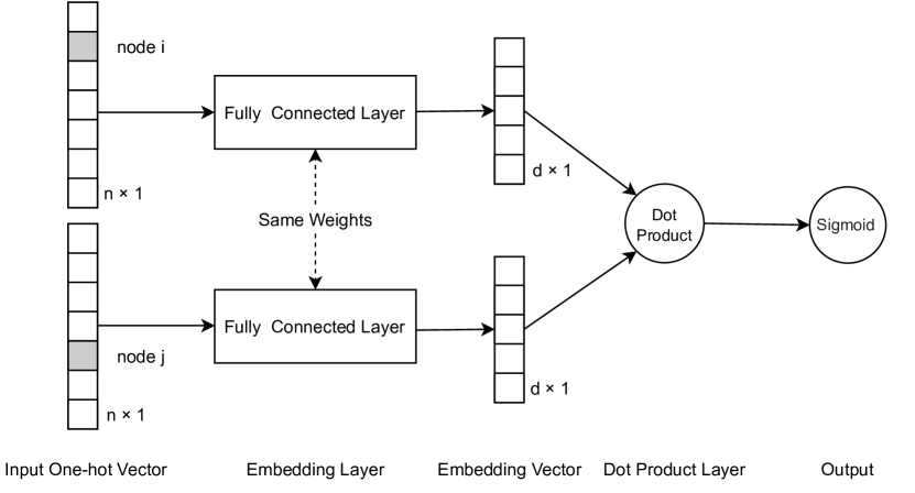
A practical approach to compute the embedding vectors of ErgoVEC can be described as follows. Given a graph and algorithm parameters w𝑤w and k𝑘k, first calculate n¯ij+superscriptsubscript¯𝑛𝑖𝑗\bar{n}_{ij}^{+}’s and n¯ijsuperscriptsubscript¯𝑛𝑖𝑗\bar{n}_{ij}^{-}’s using Theorem 1. Then use them to solve the ErgoVEC optimization problem in Equation 6 via stochastic gradient descent to find embedding vectors 𝐮isubscript𝐮𝑖\mathbf{u}_{i}’s. A neural-network implementation is described in Section 4.2 and Appendix B.

ErgoVEC calculates the coefficients of the optimization objective in a more principled way compared to VEC and completely bypasses the random walk sampling process. The r𝑟r and \ell algorithm parameters of VEC are not needed at all in ErgoVEC. However, when the graph is dense or w𝑤w is large, evaluating n¯ij+superscriptsubscript¯𝑛𝑖𝑗\bar{n}_{ij}^{+} from Eq. (4) can be computationally very expensive. In these cases, nij+superscriptsubscript𝑛𝑖𝑗n_{ij}^{+} computed from random walks could serve as an approximation. Thus VEC can may be viewed as a practical approximation to the more principled ErgoVEC.

Relationship to modularity maximization. When the graph is connected and we set w=1𝑤1w=1, Eq. (6) reduces to

argmin{𝐮i,i𝒱}(i,j)𝒱2[Aijσ(+𝐮i𝐮j)+kdidjkdkσ(𝐮i𝐮j)],subscript𝐮𝑖𝑖𝒱subscript𝑖𝑗superscript𝒱2delimited-[]subscript𝐴𝑖𝑗𝜎superscriptsubscript𝐮𝑖topsubscript𝐮𝑗𝑘subscript𝑑𝑖subscript𝑑𝑗subscript𝑘subscript𝑑𝑘𝜎superscriptsubscript𝐮𝑖topsubscript𝐮𝑗\displaystyle\underset{\{\mathbf{u}_{i},i\in\mathcal{V}\}}{\arg\min}\sum_{(i,j)\in\mathcal{V}^{2}}\left[A_{ij}\;\sigma(+\mathbf{u}_{i}^{\top}\mathbf{u}_{j})+k\frac{d_{i}d_{j}}{\sum_{k}d_{k}}\;\sigma(-\mathbf{u}_{i}^{\top}\mathbf{u}_{j})\right]\!,\!\!\!\! (7)

where disubscript𝑑𝑖d_{i} denotes the degree of node i𝑖i. If instead we set σ(t):=tassign𝜎𝑡𝑡\sigma(t)\vcentcolon=t, and constrain the embedding vectors so that for all i,j𝑖𝑗i,j, 𝐮i𝐮j{0,1}superscriptsubscript𝐮𝑖topsubscript𝐮𝑗01\mathbf{u}_{i}^{\top}\mathbf{u}_{j}\in\{0,1\}, then the minimization becomes equivalent to the modularity maximization problem [37] for two communities defined by

argmax{yi{0,1},i𝒱}(i,j)𝒱2(Aijdidj2||)1(yi=yj)formulae-sequencesubscript𝑦𝑖01𝑖𝒱subscript𝑖𝑗superscript𝒱2subscript𝐴𝑖𝑗subscript𝑑𝑖subscript𝑑𝑗21subscript𝑦𝑖subscript𝑦𝑗\displaystyle\underset{\{y_{i}\in\{0,1\},i\in\mathcal{V}\}}{\arg\max}\sum_{(i,j)\in\mathcal{V}^{2}}\left(A_{ij}-\frac{d_{i}d_{j}}{2|\mathcal{E}|}\right)1(y_{i}=y_{j})

where yisubscript𝑦𝑖y_{i} denotes the community assignment for node i𝑖i, 1()11(\cdot) is the indicator function, and |||\mathcal{E}| is the number of edges. This is often relaxed to (7) and solved via spectral approaches followed by clustering [38].

3.2 Walk-distance weighting and large r𝑟r asymptotics

Walk-distance-weighted count statistics: In VEC, nij+superscriptsubscript𝑛𝑖𝑗n_{ij}^{+} is the count of all instances where node i𝑖i appears within w𝑤w steps of node j𝑗j in all the random walks. Instances where nodes i𝑖i and j𝑗j appear exactly 111 step from each other and instances where they appear in exactly w𝑤w steps from each other, both contribute a count of 111 to the value of nij+superscriptsubscript𝑛𝑖𝑗n_{ij}^{+}. A nuanced alternative must account for the number of steps between appearances of nodes.

As a general approach to construct such a statistic, we propose associating a walk-distance weight αvsubscript𝛼𝑣\alpha_{v} to the counts of instances of node pairs that occur exactly v𝑣v steps from each other. With this modification, the walk-distance-weighted positive-pair counts will become nij+:=v=1αvnij+(v)assignsuperscriptsubscript𝑛𝑖𝑗superscriptsubscript𝑣1subscript𝛼𝑣superscriptsubscript𝑛𝑖𝑗𝑣n_{ij}^{+}:=\sum_{v=1}^{\infty}\alpha_{v}n_{ij}^{+}(v), where nij+(v)superscriptsubscript𝑛𝑖𝑗𝑣n_{ij}^{+}(v) is the count of instances where node i𝑖i appears exactly v𝑣v steps from node j𝑗j in all the random walks. The original count statistic for positive pairs can be recovered as a special case of our proposed general framework by choosing αv=1subscript𝛼𝑣1\alpha_{v}=1 for all vw𝑣𝑤v\leq w and αv=0subscript𝛼𝑣0\alpha_{v}=0 for all v>w𝑣𝑤v>w. Choosing a nonnegative decreasing sequence of walk-distance weights αvsubscript𝛼𝑣\alpha_{v} can be viewed as providing a “soft cutoff” for the bigram counts when compared to the “hard cutoff” of the original counts.

To compute walk-distance weighted counts for negative-pairs, we propose the following modification to the original negative sampling process. For each positive pair of nodes that occur exactly v𝑣v steps apart, we append k𝑘k node pairs drawn in an IID manner exactly as in the original sampling process. However, these k𝑘k negative node pairs will now contribute the value αvsubscript𝛼𝑣\alpha_{v} to the walk-distance weighted negative-pair counts as opposed to the value of 111 previously.

Large r𝑟r asymptotics: The effect of increasing \ell is similar to that of increasing r𝑟r. In a random walk on a graph, the choice of the next node depends only on the current node. From this point of view, we may loosely visualize a long random walk as being formed by joining many shorter segments which are nearly independent random walks. In this sense, an infinitely long random walk is similar to an infinite sequence of short random walks with each starting node chosen from the stationary distribution of the Markov chain. Thus, in addition to the large \ell asymptotics characterized in Theorem 1, we can also study other types of asymptotics such as r𝑟r\rightarrow\infty or, more generally, \ell and r𝑟r both going to infinity together in some manner.

The counterpart of Theorem 1 for the proposed walk-distance-weighted counts is the following general result which is proved in Appendix A.2.

Theorem 2 (Limits of walk-distance weighted counts).

Let 𝒢𝒢\mathcal{G} be a weighted connected graph with n𝑛n nodes and W𝑊W be the probability transition matrix of the natural random walk on 𝒢𝒢\mathcal{G} with stationary distribution 𝛑𝛑\bm{\pi}. Let the VEC algorithm be executed with 𝒢𝒢\mathcal{G} as input, walk-distance weights {αv}v=1superscriptsubscriptsubscript𝛼𝑣𝑣1\{\alpha_{v}\}_{v=1}^{\infty}, and negative sampling rate k𝑘k. If {αv}v=1superscriptsubscriptsubscript𝛼𝑣𝑣1\{\alpha_{v}\}_{v=1}^{\infty} is absolutely convergent, i.e., v=1|αv|<superscriptsubscript𝑣1subscript𝛼𝑣\sum_{v=1}^{\infty}|\alpha_{v}|<\infty, the following limits of n¯ij+superscriptsubscript¯𝑛𝑖𝑗\bar{n}_{ij}^{+}’s and n¯ijsuperscriptsubscript¯𝑛𝑖𝑗\bar{n}_{ij}^{-}’s exist in the almost sure sense:

  1. 1.

    When r𝑟r is fixed and \ell\rightarrow\infty (ergodic limits):

    1rnlimnij+=1𝑟𝑛subscriptsuperscriptsubscript𝑛𝑖𝑗absent\displaystyle\frac{1}{rn}\lim\limits_{\ell\rightarrow\infty}\frac{n_{ij}^{+}}{\ell}={} πiv=1αv(Wv)ij,subscript𝜋𝑖superscriptsubscript𝑣1subscript𝛼𝑣subscriptsuperscript𝑊𝑣𝑖𝑗\displaystyle\pi_{i}\sum_{v=1}^{\infty}\alpha_{v}(W^{v})_{ij}, (8)
    1rnlimnij=1𝑟𝑛subscriptsuperscriptsubscript𝑛𝑖𝑗absent\displaystyle\frac{1}{rn}\lim\limits_{\ell\rightarrow\infty}\frac{n_{ij}^{-}}{\ell}={} kπiπjv=1αv.𝑘subscript𝜋𝑖subscript𝜋𝑗superscriptsubscript𝑣1subscript𝛼𝑣\displaystyle k\pi_{i}\pi_{j}\sum_{v=1}^{\infty}\alpha_{v}. (9)
  2. 2.

    When \ell is fixed and r𝑟r\rightarrow\infty:

    1nlimrnij+r=1𝑛subscript𝑟superscriptsubscript𝑛𝑖𝑗𝑟absent\displaystyle\frac{1}{\ell n}\lim\limits_{r\rightarrow\infty}\frac{n_{ij}^{+}}{r}={} 1nm=1nv=1αv(Wv)ijs=1v(W)mis1,1𝑛superscriptsubscript𝑚1𝑛superscriptsubscript𝑣1subscript𝛼𝑣subscriptsuperscript𝑊𝑣𝑖𝑗superscriptsubscript𝑠1𝑣subscriptsuperscript𝑊𝑠1𝑚𝑖\displaystyle\frac{1}{\ell n}\sum_{m=1}^{n}\sum_{v=1}^{\infty}\alpha_{v}(W^{v})_{ij}\sum_{s=1}^{\ell-v}(W)^{s-1}_{mi}, (10)
    1nlimrnijr=1𝑛subscript𝑟superscriptsubscript𝑛𝑖𝑗𝑟absent\displaystyle\frac{1}{\ell n}\lim\limits_{r\rightarrow\infty}\frac{n_{ij}^{-}}{r}={} kπj()nm=1nv=1αvs=1v(W)mis1𝑘subscriptsuperscript𝜋𝑗𝑛superscriptsubscript𝑚1𝑛superscriptsubscript𝑣1subscript𝛼𝑣superscriptsubscript𝑠1𝑣subscriptsuperscript𝑊𝑠1𝑚𝑖\displaystyle\frac{k\pi^{(\ell)}_{j}}{\ell n}\sum_{m=1}^{n}\sum_{v=1}^{\infty}\alpha_{v}\sum_{s=1}^{\ell-v}(W)^{s-1}_{mi} (11)

    where πj()=1u=11n𝟏nWu1𝒆jsubscriptsuperscript𝜋𝑗1superscriptsubscript𝑢11𝑛superscriptsubscript1𝑛topsuperscript𝑊𝑢1subscript𝒆𝑗\pi^{(\ell)}_{j}=\frac{1}{\ell}\sum_{u=1}^{\ell}\frac{1}{n}\bm{1}_{n}^{\top}W^{u-1}\bm{e}_{j}.111We follow the convention that when the upper limit of a summation is smaller than its lower limit, the sum is 00.

  3. 3.

    Double limits:

    1nlimrlimnij+r=1nlimlimrnij+r=1𝑛subscript𝑟subscriptsuperscriptsubscript𝑛𝑖𝑗𝑟1𝑛subscriptsubscript𝑟superscriptsubscript𝑛𝑖𝑗𝑟absent\displaystyle\frac{1}{n}\lim\limits_{r\rightarrow\infty}\lim\limits_{\ell\rightarrow\infty}\frac{n_{ij}^{+}}{r\ell}={}\frac{1}{n}\lim\limits_{\ell\rightarrow\infty}\lim\limits_{r\rightarrow\infty}\frac{n_{ij}^{+}}{r\ell}={} πiv=1αv(Wv)ij,subscript𝜋𝑖superscriptsubscript𝑣1subscript𝛼𝑣subscriptsuperscript𝑊𝑣𝑖𝑗\displaystyle\pi_{i}\sum_{v=1}^{\infty}\alpha_{v}(W^{v})_{ij}, (12)
    1nlimrlimnijr=1nlimlimrnijr=1𝑛subscript𝑟subscriptsuperscriptsubscript𝑛𝑖𝑗𝑟1𝑛subscriptsubscript𝑟superscriptsubscript𝑛𝑖𝑗𝑟absent\displaystyle\frac{1}{n}\lim\limits_{r\rightarrow\infty}\lim\limits_{\ell\rightarrow\infty}\frac{n_{ij}^{-}}{r\ell}={}\frac{1}{n}\lim\limits_{\ell\rightarrow\infty}\lim\limits_{r\rightarrow\infty}\frac{n_{ij}^{-}}{r\ell}={} kπiπjv=1αv.𝑘subscript𝜋𝑖subscript𝜋𝑗superscriptsubscript𝑣1subscript𝛼𝑣\displaystyle k\pi_{i}\pi_{j}\sum_{v=1}^{\infty}\alpha_{v}. (13)

Theorem 2 is stated for a connected graph, but it holds for each connected component of a disconnected graph. The main changes are that the expressions πiv=1w(Wv)ijsubscript𝜋𝑖superscriptsubscript𝑣1𝑤subscriptsuperscript𝑊𝑣𝑖𝑗\pi_{i}\sum_{v=1}^{w}(W^{v})_{ij} and kπiπjw𝑘subscript𝜋𝑖subscript𝜋𝑗𝑤k\pi_{i}\pi_{j}w in Lemma 1 change to πiv=1αv(Wv)ijsubscript𝜋𝑖superscriptsubscript𝑣1subscript𝛼𝑣subscriptsuperscript𝑊𝑣𝑖𝑗\pi_{i}\sum_{v=1}^{\infty}\alpha_{v}(W^{v})_{ij} and kπiπj(v=1αvk\pi_{i}\pi_{j}(\sum_{v=1}^{\infty}\alpha_{v}) respectively and the large-r𝑟r asymptotic limits of the normalized count statistics are also characterized. To establish these results, we need to assume that the walk-distance weight series is absolutely convergent. Walk-distance weighting makes it possible to realize different nonlinear functions of the transition matrix as the ergodic limit of count statistics, not just polynomial functions. For instance, if we choose αv=1/v!subscript𝛼𝑣1𝑣\alpha_{v}=\nicefrac{{1}}{{v!}} for all v𝑣v, then for all i,j𝑖𝑗i,j, n¯ij+=πi(exp{W})ijsuperscriptsubscript¯𝑛𝑖𝑗subscript𝜋𝑖subscript𝑊𝑖𝑗\bar{n}_{ij}^{+}=\pi_{i}(\exp\{W\})_{ij}, where exp{W}𝑊\exp\{W\} denotes matrix exponential, and n¯ij=kπiπjesuperscriptsubscript¯𝑛𝑖𝑗𝑘subscript𝜋𝑖subscript𝜋𝑗𝑒\bar{n}_{ij}^{-}=k\pi_{i}\pi_{j}e. We note that the large-\ell asymptotic limits are independent of r𝑟r but the large-r𝑟r asymptotic limits depend on \ell. Yet, the double limits where r𝑟r is sent to infinity first before \ell equal the corresponding large-\ell limits.

3.3 Reparameterized relaxations and their properties

In this subsection, we study matrix re-parameterizations and convex relaxations of the VEC and ErgoVEC optimization problems. We follow [35] and begin by defining the n×n𝑛𝑛n\times n matrix X𝑋X to be the Gram matrix of the node embedding vectors, i.e., for all i,j𝑖𝑗i,j, Xij:=𝐮i𝐮jassignsubscript𝑋𝑖𝑗superscriptsubscript𝐮𝑖topsubscript𝐮𝑗X_{ij}:=\mathbf{u}_{i}^{\top}\mathbf{u}_{j}. Let N+superscript𝑁N^{+} and Nsuperscript𝑁N^{-} denote the n×n𝑛𝑛n\times n matrices of the positive-pair and negative-pair counts respectively, i.e., for all i,j𝑖𝑗i,j, [N+]ij=nij+subscriptdelimited-[]superscript𝑁𝑖𝑗superscriptsubscript𝑛𝑖𝑗[N^{+}]_{ij}=n_{ij}^{+} and [N]ij:=nijassignsubscriptdelimited-[]superscript𝑁𝑖𝑗superscriptsubscript𝑛𝑖𝑗[N^{-}]_{ij}:=n_{ij}^{-}. If

f(N+,\displaystyle f(N^{+}, N,X):=(i,j)𝒱2nij+σ(+Xij)+(i,j)𝒱2nijσ(Xij),\displaystyle N^{-},X)\vcentcolon={}\!\!\!\!\sum_{(i,j)\in\mathcal{V}^{2}}n_{ij}^{+}\sigma(+X_{ij})+\sum_{(i,j)\in\mathcal{V}^{2}}n_{ij}^{-}\sigma(-X_{ij}),

then the VEC optimization problem (Eq. (1)) reduces to the following equivalent optimization problem in the matrix variable X𝑋X named GramVEC:

Definition 4 (GramVEC optimization objective).
argminX𝕊+n,rank(X)df(N+,N,X).subscriptargminformulae-sequence𝑋subscriptsuperscript𝕊𝑛rank𝑋𝑑𝑓superscript𝑁superscript𝑁𝑋\operatornamewithlimits{argmin}_{X\in\mathbb{S}^{n}_{+},\ \mathrm{rank}(X)\leq d}f(N^{+},N^{-},X). (14)

In Eq. (14), the constraint X𝕊+n𝑋subscriptsuperscript𝕊𝑛X\in\mathbb{S}^{n}_{+} arises from the fact that the Gram matrix of embedding vectors is real, symmetric, and positive semi-definite. The rank constraint comes from the fact that 𝐮idsubscript𝐮𝑖superscript𝑑\mathbf{u}_{i}\in\mathbb{R}^{d}. The equivalence of the VEC (Eq. (1)) and GramVEC (Eq. (14)) optimization problems can be seen as follows. For any set of feasible 𝐮isubscript𝐮𝑖\mathbf{u}_{i}’s in (1), setting Xij=𝐮i𝐮jsubscript𝑋𝑖𝑗superscriptsubscript𝐮𝑖topsubscript𝐮𝑗X_{ij}=\mathbf{u}_{i}^{\top}\mathbf{u}_{j} for all i,j𝑖𝑗i,j, makes X𝑋X a rank-d𝑑d matrix in 𝕊+nsubscriptsuperscript𝕊𝑛\mathbb{S}^{n}_{+} and yields the same cost as in (14). In the other direction, for any feasible choice of X𝑋X in (14), let X=VdΣdVd𝑋subscriptsuperscript𝑉top𝑑subscriptΣ𝑑subscript𝑉𝑑X=V^{\top}_{d}\Sigma_{d}V_{d} denote its rank-d𝑑d reduced SVD with diagonal Σd𝕊+dsubscriptΣ𝑑subscriptsuperscript𝕊𝑑\Sigma_{d}\in\mathbb{S}^{d}_{+} and define U=[𝐮1,,𝐮n]:=ΣdVd𝑈subscript𝐮1subscript𝐮𝑛assignsubscriptΣ𝑑subscript𝑉𝑑U=[\mathbf{u}_{1},\ldots,\mathbf{u}_{n}]:=\sqrt{\Sigma_{d}}V_{d}. Then, X=UU𝑋superscript𝑈top𝑈X=U^{\top}U and for all i,j𝑖𝑗i,j, Xij=𝐮i𝐮jsubscript𝑋𝑖𝑗superscriptsubscript𝐮𝑖topsubscript𝐮𝑗X_{ij}=\mathbf{u}_{i}^{\top}\mathbf{u}_{j} and 𝐮idsubscript𝐮𝑖superscript𝑑\mathbf{u}_{i}\in\mathbb{R}^{d}, and we obtain the same cost in (1). The choices for the 𝐮isubscript𝐮𝑖\mathbf{u}_{i}’s are not unique since X=UFFU𝑋superscript𝑈topsuperscript𝐹top𝐹𝑈X=U^{\top}F^{\top}FU for any real orthonormal matrix F𝐹F. The 𝐮isubscript𝐮𝑖\mathbf{u}_{i}’s are unique only up to a real orthonormal transformation, just as in (1).

The same re-parameterization can also be applied to ErgoVEC (Eq. (6)). Let N¯+superscript¯𝑁\bar{N}^{+} and N¯superscript¯𝑁\bar{N}^{-} be n×n𝑛𝑛n\times n matrices such that for all i,j𝑖𝑗i,j, [N¯+]ij:=n¯ij+assignsubscriptdelimited-[]superscript¯𝑁𝑖𝑗superscriptsubscript¯𝑛𝑖𝑗[\bar{N}^{+}]_{ij}:=\bar{n}_{ij}^{+} and [N¯]ij:=n¯ijassignsubscriptdelimited-[]superscript¯𝑁𝑖𝑗superscriptsubscript¯𝑛𝑖𝑗[\bar{N}^{-}]_{ij}:=\bar{n}_{ij}^{-}. Then the GramErgoVEC optimization problem is defined as follows.

Definition 5 (GramErgoVEC optimization problem).
argminX𝕊+n,rank(X)df(N¯+,N¯,X).subscriptargminformulae-sequence𝑋subscriptsuperscript𝕊𝑛rank𝑋𝑑𝑓superscript¯𝑁superscript¯𝑁𝑋\operatornamewithlimits{argmin}_{X\in\mathbb{S}^{n}_{+},\ \mathrm{rank}(X)\leq d}f(\bar{N}^{+},\bar{N}^{-},X). (15)

Although Eq. (14) and Eq. (15) are equivalent to Eq. (1) and Eq. (6), respectively, they are more convenient to work with and analyze. The matrix re-parameterization transfers the non-convexity from the objective function to the constraint set which makes it possible to relax or convexify the problem as we do next.

Relaxing all constraints on X𝑋X in GramErgoVEC leads to the following optimization problem named GramErgoPMI (relaxing constraints in GramVEC similarly will yield a corresponding optimization problem GramPMI):

Definition 6 (GramErgoPMI optimization problem).
argminXn×nf(N¯+,N¯,X).subscriptargmin𝑋superscript𝑛𝑛𝑓superscript¯𝑁superscript¯𝑁𝑋\operatornamewithlimits{argmin}_{X\in\mathbb{R}^{n\times n}}f(\bar{N}^{+},\bar{N}^{-},X). (16)

In general, GramErgoPMI is not equivalent to GramErgoVEC. The relaxation enlarges the feasible set and the optimal solution may not satisfy the constraints in Eq.(15). Nonetheless, Eq. (16) admits a closed-form solution:

Proposition 1.

Let Xsuperscript𝑋X^{*} be the solution to Eq. (16). Then, Xsuperscript𝑋X^{*} is unique, symmetric, and given by

Xij=Xji={ln(n¯ij+n¯ij)if n¯ij+0;if n¯ij+=0.superscriptsubscript𝑋𝑖𝑗superscriptsubscript𝑋𝑗𝑖casessuperscriptsubscript¯𝑛𝑖𝑗superscriptsubscript¯𝑛𝑖𝑗if superscriptsubscript¯𝑛𝑖𝑗0if superscriptsubscript¯𝑛𝑖𝑗0X_{ij}^{*}=X_{ji}^{*}=\begin{cases}\ln\left(\frac{\bar{n}_{ij}^{+}}{\bar{n}_{ij}^{-}}\right)&\text{if }\bar{n}_{ij}^{+}\neq 0;\\ -\infty&\text{if }\bar{n}_{ij}^{+}=0.\end{cases} (17)

Let p(i,j)subscript𝑝𝑖𝑗p_{\ell}(i,j) denote the probability that a randomly sampled pair from the positive set 𝒟+subscript𝒟\mathcal{D}_{+} equals (i,j)𝑖𝑗(i,j) and let p1(i)subscript𝑝1𝑖p_{\ell 1}(i) and p2(j)subscript𝑝2𝑗p_{\ell 2}(j) denote, respectively, the first- and second-component marginal probabilities of i𝑖i and j𝑗j that are consistent with the joint pmf p(i,j)subscript𝑝𝑖𝑗p_{\ell}(i,j).222That is, p1(i):=j𝒱p(i,j)assignsubscript𝑝1𝑖subscript𝑗𝒱subscript𝑝𝑖𝑗p_{\ell 1}(i):=\sum_{j\in\mathcal{V}}p_{\ell}(i,j) and p2(j):=i𝒱p(i,j)assignsubscript𝑝2𝑗subscript𝑖𝒱subscript𝑝𝑖𝑗p_{\ell 2}(j):=\sum_{i\in\mathcal{V}}p_{\ell}(i,j). Note that p(i,j)subscript𝑝𝑖𝑗p_{\ell}(i,j) may not be symmetric when \ell is finite. Let PMI(i,j):=ln(p(i,j)p1(i)p2(j))assignsubscriptPMI𝑖𝑗subscript𝑝𝑖𝑗subscript𝑝1𝑖subscript𝑝2𝑗\text{PMI}_{\ell}(i,j):=\ln\left(\frac{p_{\ell}(i,j)}{p_{\ell 1}(i)p_{\ell 2}(j)}\right) denote the Pointwise Mutual Information (PMI) of (i,j)𝑖𝑗(i,j) [36]. Then for all i,j𝑖𝑗i,j,

Xij=limPMI(i,j)lnk.superscriptsubscript𝑋𝑖𝑗subscriptsubscriptPMI𝑖𝑗𝑘X_{ij}^{*}=\lim_{\ell\rightarrow\infty}\text{PMI}_{\ell}(i,j)-\ln{k}. (18)

The proof of Proposition 1 is presented in Appendix A.3. Although Xsuperscript𝑋X^{*} is symmetric, there is no guarantee that Xsuperscript𝑋X^{*} will satisfy the positive semi-definiteness constraint of GramErgoVEC, let alone the rank constraint. Without positive semi-definiteness, the square root of Xsuperscript𝑋X^{*}’s nonzero singular values will be imaginary and there will not exist any real-valued embedding vectors, even in nsuperscript𝑛\mathbb{R}^{n}, whose Gram matrix equals Xsuperscript𝑋X^{*}. A practical solution then is to compute the 2subscript2\ell_{2} projection of Xsuperscript𝑋X^{*} into the rank-d𝑑d real positive semi-definite cone of n×n𝑛𝑛n\times n matrices and factorize the projected matrix Proj(X,d)Projsuperscript𝑋𝑑\text{Proj}(X^{*},d) to get embeddings. Still, there is no guarantee that the projected matrix Proj(X,d)Projsuperscript𝑋𝑑\text{Proj}(X^{*},d) or the embeddings 𝐮isubscript𝐮𝑖\mathbf{u}_{i}’s obtained from it will be a solution to GramErgoVEC. We compare the GramErgoVEC and GramErgoPMI embedding vectors experimentally in Section 5.

An alternative approach to deal with the non-convexity of the GramErgoVEC is to replace the non-convex rank constraint with a nuclear norm constraint which is convex. The nuclear norm Xsubscriptnorm𝑋\|X\|_{*} of a matrix X𝑋X is defined as the sum of its singular values. Its relationship with the rank of a matrix has been extensively studied in the literature. For example, nuclear norm level sets have been shown to be the convex-envelope of rank level sets[39]. A bounded nuclear norm constraint has been used as a proxy for a bounded rank constraint in a number of problems such as low rank matrix completion [40], tensor robust PCA [41], and compressed sensing [42]. For some problems there exists an exact equivalence between these constraints but the conditions under which this occurs varies from problem to problem. Relaxing the rank constraint of GramErgoVEC via a bound on the nuclear norm leads to the following optimization problem that we term NucGramErgoVEC (we can similarly define NucGramVEC):

Definition 7 (NucGramErgoVEC optimization problem).
argminX𝕊+n,Xνnf(N¯+,N¯,X)subscriptargminformulae-sequence𝑋subscriptsuperscript𝕊𝑛subscriptnorm𝑋subscript𝜈𝑛𝑓superscript¯𝑁superscript¯𝑁𝑋\operatornamewithlimits{argmin}_{X\in\mathbb{S}^{n}_{+},\ \|X\|_{*}\leq\nu_{n}}f(\bar{N}^{+},\bar{N}^{-},X) (19)

A larger νnsubscript𝜈𝑛\nu_{n} implies a looser nuclear norm constraint. When νnsubscript𝜈𝑛\nu_{n} goes to \infty, the solution to NucGramErgoVEC will approach the 2subscript2\ell_{2} projection of the GramErgoPMI solution onto the real positive semi-definite cone of n×n𝑛𝑛n\times n matrices. However, when νnsubscript𝜈𝑛\nu_{n} goes to 00, the solution to NucGramErgoVEC will reduce to the all zeros matrix which has rank 00. In general, we should expect smaller values of νnsubscript𝜈𝑛\nu_{n} to yield solutions with approximately lower rank. This is corroborated by our experiments in Section 5.1. Thus the rank of the solution matrix, and consequently the dimension of the embedding vectors, can be controlled by the value of νnsubscript𝜈𝑛\nu_{n}. Note that we allow the nuclear norm threshold νnsubscript𝜈𝑛\nu_{n} to depend on n𝑛n. In Section 3.4 we show that the nuclear norms of the solutions to GramErgoPMI and GramErgoVEC for idealized graphs that have community structure scale with n𝑛n as νn=Θ(n)subscript𝜈𝑛Θ𝑛\nu_{n}=\Theta(n).

There are numerous algorithms available to numerically compute a solution to the NucGramErgoVEC optimization problem. We modified and implemented Hazan’s algorithm [43] to generate all our experimental results.

3.4 Embeddings of expected SBM graphs

As an important step toward analyzing concentration properties of embeddings, in this section we study the embedding solutions of different optimization problems focusing on the expected graph of a two-community SBM. Such graphs have an ideal community structure: all edges between nodes belonging to any specified pair of communities have the same edge weight. Our main result is summarized in the following theorem:

Theorem 3 (Embeddings of an expected SBM graph).

Let 𝒢𝒢\mathcal{G} be an SBM graph with n=2m𝑛2𝑚n=2m, m2𝑚2m\geq 2, nodes and two balanced communities. For all i𝒱𝑖𝒱i\in\mathcal{V}, let yi{0,1}subscript𝑦𝑖01y_{i}\in\{0,1\} denote the community label of node i𝑖i. Let a𝑎a and b𝑏b be the edge forming probabilities for within- and cross-community edges, respectively, with a>mm1b𝑎𝑚𝑚1𝑏a>\frac{m}{m-1}b. Let 𝐄[𝒢]𝐄delimited-[]𝒢\mathbf{E}[\mathcal{G}] denote the expected graph and n¯ij+superscriptsubscript¯𝑛𝑖𝑗\bar{n}_{ij}^{+}’s and n¯ijsuperscriptsubscript¯𝑛𝑖𝑗\bar{n}_{ij}^{-}’s the ergodic limits for 𝐄[𝒢]𝐄delimited-[]𝒢\mathbf{E}[\mathcal{G}] as in Definition 2, with k1𝑘1k\geq 1 and w1𝑤1w\geq 1. Let

X():=argminXf(N¯+,N¯,X),assignsuperscript𝑋subscriptargmin𝑋𝑓superscript¯𝑁superscript¯𝑁𝑋\displaystyle X^{*}(\mathcal{H}):=\operatornamewithlimits{argmin}_{X\in\mathcal{H}}f(\bar{N}^{+},\bar{N}^{-},X), (20)

where n×nsuperscript𝑛𝑛\mathcal{H}\subset\mathbb{R}^{n\times n}. Let 0:={(i,j):yi=yj}assignsubscript0conditional-set𝑖𝑗subscript𝑦𝑖subscript𝑦𝑗\mathcal{E}_{0}:=\left\{(i,j)\in\mathcal{E}:y_{i}=y_{j}\right\} and 1:=\0assignsubscript1\subscript0\mathcal{E}_{1}:=\mathcal{E}\backslash\mathcal{E}_{0}. Then:

  1. 1.

    Structure of ergodic limits: The values of n¯ij+superscriptsubscript¯𝑛𝑖𝑗\bar{n}_{ij}^{+} and n¯ijsuperscriptsubscript¯𝑛𝑖𝑗\bar{n}_{ij}^{-} depend only on the community membership of (i,j)𝑖𝑗(i,j), i.e.,

    n¯ij+superscriptsubscript¯𝑛𝑖𝑗\displaystyle\bar{n}_{ij}^{+} ={α1,if (i,j)0α2,if (i,j)1α3,if i=jabsentcasessubscript𝛼1if (i,j)0subscript𝛼2if (i,j)1subscript𝛼3if i=j\displaystyle=\begin{cases}\alpha_{1},&\text{if $(i,j)\in\mathcal{E}_{0}$}\\ \alpha_{2},&\text{if $(i,j)\in\mathcal{E}_{1}$}\\ \alpha_{3},&\text{if $i=j$}\end{cases}
    n¯ijsuperscriptsubscript¯𝑛𝑖𝑗\displaystyle\bar{n}_{ij}^{-} =β,(i,j),absent𝛽for-all𝑖𝑗\displaystyle=\beta,\quad\forall(i,j),

    where β=kwn2𝛽𝑘𝑤superscript𝑛2\beta=\frac{kw}{n^{2}} and αi=Ci/n2+o(1/n2)subscript𝛼𝑖subscript𝐶𝑖superscript𝑛2𝑜1superscript𝑛2\alpha_{i}=C_{i}/n^{2}+o(1/n^{2}) for i=1,2,3𝑖123i=1,2,3, where Cisubscript𝐶𝑖C_{i}’s are functions of only a𝑎a, b𝑏b and w𝑤w.

  2. 2.

    GramErgoPMI solution: Let =n×nsuperscript𝑛𝑛\mathcal{H}=\mathbb{R}^{n\times n}. Then X()superscript𝑋X^{*}(\mathcal{H}) has full rank with the same structure as n¯ij+superscriptsubscript¯𝑛𝑖𝑗\bar{n}_{ij}^{+} with

    X(n×n)superscript𝑋superscript𝑛𝑛\displaystyle X^{*}(\mathbb{R}^{n\times n}) ={ln(α1β),if (i,j)0ln(α2β),if (i,j)1ln(α3β),if i=jabsentcasessubscript𝛼1𝛽if (i,j)0subscript𝛼2𝛽if (i,j)1subscript𝛼3𝛽if i=j\displaystyle=\begin{cases}\ln\left(\frac{\alpha_{1}}{\beta}\right),&\text{if $(i,j)\in\mathcal{E}_{0}$}\\ \ln\left(\frac{\alpha_{2}}{\beta}\right),&\text{if $(i,j)\in\mathcal{E}_{1}$}\\ \ln\left(\frac{\alpha_{3}}{\beta}\right),&\text{if $i=j$}\end{cases}
  3. 3.

    NucGramErgoVEC solution for νn=subscript𝜈𝑛\nu_{n}=\infty: Let =𝕊+nsubscriptsuperscript𝕊𝑛\mathcal{H}=\mathbb{S}^{n}_{+} and ν1:=ln(α¯13+βα2+β)assignsubscript𝜈1subscript¯𝛼13𝛽subscript𝛼2𝛽\nu_{1}:=\ln\left(\frac{\bar{\alpha}_{13}+\beta}{\alpha_{2}+\beta}\right) where α¯13:=m1mα1+1mα3assignsubscript¯𝛼13𝑚1𝑚subscript𝛼11𝑚subscript𝛼3\bar{\alpha}_{13}\vcentcolon=\frac{m-1}{m}\alpha_{1}+\frac{1}{m}\alpha_{3}. Then X()superscript𝑋X^{*}(\mathcal{H}) has rank 111. Moreover, if νn=ν1nsubscript𝜈𝑛subscript𝜈1𝑛\nu_{n}=\nu_{1}n, then

    X(𝕊+n)superscript𝑋subscriptsuperscript𝕊𝑛\displaystyle X^{*}(\mathbb{S}^{n}_{+}) ={ν1,if (i,j)0 or i=jν1,if (i,j)1.absentcasessubscript𝜈1if (i,j)0 or i=jsubscript𝜈1if (i,j)1\displaystyle=\begin{cases}\phantom{-}\nu_{1},&\text{if $(i,j)\in\mathcal{E}_{0}$ or $i=j$}\\ -\nu_{1},&\text{if $(i,j)\in\mathcal{E}_{1}$}.\end{cases}
  4. 4.

    The nuclear norms of X(n×n)superscript𝑋superscript𝑛𝑛X^{*}(\mathbb{R}^{n\times n}) and X(𝕊+n)superscript𝑋subscriptsuperscript𝕊𝑛X^{*}(\mathbb{S}^{n}_{+}) scale with n𝑛n as Θ(n)Θ𝑛\Theta(n).

The full proof of Theorem 3 is presented in Appendix A.4, but the key ideas are as follows. Part 1)1) holds as a result of Theorem 1 which characterizes the ergodic limits of normalized bigram counts in terms of the random walk transition matrix. Since the transition matrix of the expected graph has block-wise constant entries, this property is carried forward to the normalized ergodic counts. Part 2)2) follows directly from part 1)1) and Proposition 1. Part 3)3) is the major piece of this theorem and is proved via an intricate analysis of the structure of the solution.

The Θ(n)Θ𝑛\Theta(n) scaling of nuclear norms of X(n×n)superscript𝑋superscript𝑛𝑛X^{*}(\mathbb{R}^{n\times n}) and X(𝕊+n)superscript𝑋subscriptsuperscript𝕊𝑛X^{*}(\mathbb{S}^{n}_{+}) arises from the block structure and the fact that all entries are of constant order. Theorem 3 also shows that N¯+superscript¯𝑁\bar{N}^{+} and X(n×n)superscript𝑋superscript𝑛𝑛X^{*}(\mathbb{R}^{n\times n}), the solution to GramErgoPMI, have the structure of a rank 222 matrix minus a scalar multiple of the identity matrix making them full rank. In contrast, X(𝕊+n)superscript𝑋subscriptsuperscript𝕊𝑛X^{*}(\mathbb{S}^{n}_{+}), the solution to NucGramErgoVEC, has rank 111 due to the positive semi-definite constraint.

Part 3)3) of Theorem 3 may seem surprising on first glance because we are getting a rank 111 solution without any rank or nuclear norm constraints. The surprise dissipates when we note that the solution is for an expected graph which has an ideal community structure. Such a result would not hold true for a random graph realization. Nonetheless, we can directly obtain the GramErgoVEC and NucGramErgoVEC solutions for the expected graph from part 3)3) of Theorem 3:

Corollary 1.

Under the assumptions of Theorem 3,

  1. 1.

    GramErgoVEC solution for any positive rank: Let ={X𝕊+n:rank(X)d}conditional-set𝑋subscriptsuperscript𝕊𝑛rank𝑋𝑑\mathcal{H}=\{X\in\mathbb{S}^{n}_{+}:\text{rank}(X)\leq d\} with d1𝑑1d\geq 1. Then X()superscript𝑋X^{*}(\mathcal{H}) has rank 111 and equals the GramErgoVEC solution for νn=subscript𝜈𝑛\nu_{n}=\infty characterized in part 3) of Theorem 3.

  2. 2.

    NucGramErgoVEC solution for all νnν1nsubscript𝜈𝑛subscript𝜈1𝑛\nu_{n}\geq\nu_{1}n: Let ={X𝕊+n:Xνn}conditional-set𝑋subscriptsuperscript𝕊𝑛subscriptnorm𝑋subscript𝜈𝑛\mathcal{H}=\{X\in\mathbb{S}^{n}_{+}:\|X\|_{*}\leq\nu_{n}\}. If νnν1nsubscript𝜈𝑛subscript𝜈1𝑛\nu_{n}\geq\nu_{1}n, then X()superscript𝑋X^{*}(\mathcal{H}) has rank 111 and equals the GramErgoVEC solution for νn=subscript𝜈𝑛\nu_{n}=\infty characterized in part 3) of Theorem 3.

When given the expected SBM graph as input, GramErgoVEC and NucGramErgoVEC will return a Gram matrix of rank 111 or 222 which when factorized will provide two distinct embedding vectors, each representing one community in the original graph. In short, the algorithms will give embeddings that are perfectly separated across communities and perfectly concentrated within communities.

In part 2)2) of Corollary 1, with νnν1nsubscript𝜈𝑛subscript𝜈1𝑛\nu_{n}\geq\nu_{1}n, the nuclear norm constraint becomes inactive. Suppose that νn=ν0nsubscript𝜈𝑛subscript𝜈0𝑛\nu_{n}=\nu_{0}n. If ν0ν1subscript𝜈0subscript𝜈1\nu_{0}\leq\nu_{1}, we conjecture that the solution will scale proportionally with ν0subscript𝜈0\nu_{0}:

Conjecture 1.

Under the assumptions of Theorem 3, let ={X𝕊+n:Xν0n}conditional-set𝑋subscriptsuperscript𝕊𝑛subscriptnorm𝑋subscript𝜈0𝑛\mathcal{H}=\{X\in\mathbb{S}^{n}_{+}:\|X\|_{*}\leq\nu_{0}n\}. If ν0<ν1subscript𝜈0subscript𝜈1\nu_{0}<\nu_{1}, then

X()superscript𝑋\displaystyle X^{*}(\mathcal{H}) ={ν0,if (i,j)0 or i=jν0,if (i,j)1.absentcasessubscript𝜈0if (i,j)0 or i=jsubscript𝜈0if (i,j)1\displaystyle=\begin{cases}\phantom{-}\nu_{0},&\text{if $(i,j)\in\mathcal{E}_{0}$ or $i=j$}\\ -\nu_{0},&\text{if $(i,j)\in\mathcal{E}_{1}$}.\end{cases}

Conjecture 1 makes an assertion about the solution to the NucGramErgoVEC optimization problem when the nuclear norm constraint is active. For a suitable nuclear norm constraint, we conjecture that the solution will be a scaling of the solution in part 3) of Theorem 3. If this conjecture holds, then, we can conclude that the solution to NucGramErgoVEC is always rank 111 with perfect separation of the communities regardless of the sparsity level of the graph. This would provide a solid starting point for analyzing the concentration properties of solutions as n𝑛n increases to \infty.

4 Experimental setup

In the following sections, we compare the node embeddings from different algorithms qualitatively and quantitatively through extensive experiments. This section details our experimental setup, including the generation of random graphs, details of implementation and parameter choices for algorithms, and evaluation metrics for embedding vectors. Section 5.1 explores the geometric properties of embedding vectors for a fixed graph size. Specifically, we study how the nuclear norm linear scaling factor ν0subscript𝜈0\nu_{0} of the nuclear norm limit νn=ν0nsubscript𝜈𝑛subscript𝜈0𝑛\nu_{n}=\nu_{0}n impacts the embedding geometry in NucGramErgoVEC. In Section 5.2 we investigate how embedding vectors change as the graph size n𝑛n increases and whether they tend to concentrate.

4.1 SBM graph generation

For simplicity, we focus on assortative, equal-sized, planted-partition SBM graphs with 2 communities. We generate random graphs with n=100,200,500,1000𝑛1002005001000n=100,200,500,1000 nodes. We consider two scaling regimes for the within-community edge forming probability p𝑝p and the cross-community edge forming probability q𝑞q: 1) Linear regime: Here, p𝑝p and q𝑞q are held constant, with values p=0.6𝑝0.6p=0.6 and q=0.06𝑞0.06q=0.06, for all graph sizes. As a result, the expected node degree scales linearly with n𝑛n. 2) Logarithmic regime: Here, p𝑝p and q𝑞q diminish with increasing graph size n𝑛n as a multiple of (lnn)/n𝑛𝑛(\ln{n})/n, specifically as p=9(lnn)/n𝑝9𝑛𝑛p=9(\ln{n})/n and q=2(lnn)/n𝑞2𝑛𝑛q=2(\ln{n})/n. The expected node degree then increases proportionally with lnn𝑛\ln{n}. Our choices of scaling factors p~=9~𝑝9\tilde{p}=9 and q~=2~𝑞2\tilde{q}=2 in the logarithmic regime ensure that the information-theoretic threshold for exact community recovery for two communities, given by p~q~>2~𝑝~𝑞2\sqrt{\tilde{p}}-\sqrt{\tilde{q}}>\sqrt{2}  [30], is slightly surpassed.

To ensure graph connectivity and improve community detection performance, we follow the prescription in [44] and apply ε𝜀\varepsilon-smoothing to all generated graphs. For a given ε0𝜀0\varepsilon\geq 0, the ε𝜀\varepsilon-smoothing of 𝒢𝒢\mathcal{G}, denoted by 𝒢εsuperscript𝒢𝜀\mathcal{G}^{\varepsilon}, is the weighted complete graph with adjacency matrix Aεsuperscript𝐴𝜀A^{\varepsilon}, where for all i,j𝑖𝑗i,j, Aijε:=Aij+εassignsubscriptsuperscript𝐴𝜀𝑖𝑗subscript𝐴𝑖𝑗𝜀A^{\varepsilon}_{ij}:=A_{ij}+\varepsilon. In addition to analytical convenience, graph-smoothing also improves the performance of spectral clustering in practice [44]. The ergodic limit of the coefficients under ε𝜀\varepsilon-smoothed graphs can be computed by Theorem 1 with a modified probability transition matrix Wεsubscript𝑊𝜀W_{\varepsilon} that corresponds to the new graph.

The optimal choice of ε𝜀\varepsilon for various performance measures such as signal-to-noise ratio, community detection accuracy, etc., varies across different random graph realizations and embedding algorithms. Since our focus is on embedding algorithms, we apply ε𝜀\varepsilon-smoothing to all random graphs that we generate with the fixed choice ε=1/10n𝜀110𝑛\varepsilon=\nicefrac{{1}}{{10n}} instead of optimizing ε𝜀\varepsilon for each algorithm and each performance measure. This is a relatively small value of ε𝜀\varepsilon as it changes the degrees from the original graph by at most 1/10110\nicefrac{{1}}{{10}} whereas the expected degrees in the linear and logarithmic regimes scale as n𝑛n and ln(n)𝑛\ln(n), respectively.

4.2 Algorithm parameter choices and implementation

We implement and compare ErgoVEC, GramErgoPMI, and NucGramErgoVEC, that were proposed in Section 3, with VEC and Spectral Clustering (SC). SC serves as a classical benchmark due to its widespread usage.

Parameter choices. For ease of visualization, we compute and plot 2-dimensional embedding vectors for all algorithms, i.e. d=2𝑑2d=2.

For all algorithms other than SC, we set the window size to w=8𝑤8w=8, and the negative sampling rate to k=5𝑘5k=5. Settings that are specific to SC, VEC, and NucGramErgoVEC are as follows:

  1. 1.

    SC: We use the first two eigenvectors of the symmetrically normalized Laplacian, i.e., D1/2AD1/2superscript𝐷12𝐴superscript𝐷12D^{-1/2}AD^{-1/2}, [45]. Since the unit-norm eigenvectors are in nsuperscript𝑛\mathbb{R}^{n}, their components, and therefore also the node embedding vectors, scale as O(1/n)𝑂1𝑛O(1/\sqrt{n}). In order to simultaneously visualize and compare embedding vectors across different values of n𝑛n, we scale them by n𝑛\sqrt{n}.

  2. 2.

    VEC: We launch r=10𝑟10r=10 walks starting from each node, each of length =100100\ell=100.

  3. 3.

    NucGramErgoVEC: In light of the linear scaling of the nuclear norm of the gram matrix of node embedding vectors for an expected SBM graph, (cf. Theorem 3 and Corollary 1), we set νn=ν0nsubscript𝜈𝑛subscript𝜈0𝑛\nu_{n}=\nu_{0}n and sweep ν0subscript𝜈0\nu_{0} over the range 0.0180.0180.018 through 0.2160.2160.216, in steps of 0.0180.0180.018, in order to illustrate changes in the geometric structure of embedding vectors (cf. Fig. 4 and Fig. 5).

Implementation of VEC and ErgoVEC. Both VEC and ErgoVEC have non-convex objectives for which there is no optimization procedure available which guarantees convergence to a global minimizer. A practical way forward is to use Stochastic Gradient Descent (SGD). We can consider two distinct approaches for implementing SGD in VEC or ErgoVEC 1) Map them to an equivalent Word2Vec problem by identifying nodes as words and random walks as sentences and then obtain word embeddings using a Word2Vec package such as Gensim [46]. 2) Reformulate each optimization problem as the training of a neural network with an appropriate architecture and cost and then train the neural network using a neural network package such as Keras [47]. Since the Gensim package cannot handle non-integer coefficients that arise in ErgoVEC, we use Keras to implement ErgoVEC and VEC. Details of our neural network implementation are presented in Appendix B. In section 5.2 we also compare the Gensim and Keras implementations of VEC.

Since both algorithms involve optimizing non-convex objectives, convergence is not guaranteed. We assess the convergence of the objective function value and the solution by evaluating the change in the objective function value and the embeddings after each epoch. To quantify the change in embeddings, we first perform a Procrustes alignment of the embedding solutions from successive epochs and then compute the Frobenius norm of the difference between the aligned sets of embeddings. We found that the change in the objective function value diminishes as the number of epochs increases, but the change in the corresponding embeddings retains a small fluctuation after diminishing initially (cf. Appendix B). This suggests that although the objective function value converges, the embeddings may be oscillating around a local optimizer. Note that the Keras implementation, which implements SGD, is not designed to minimize changes in the solution (arguments), but rather in the objective function.

Implementation of NucGramErgoVEC. We use Hazan’s algorithm [43] (suitably modified to handle inequality constraints) to solve the NucGramErgoVEC optimization problem. The algorithm is iterative and is guaranteed to converge to the global minimum. We also empirically confirmed the convergence of both the objective function value and the solution matrix using the approach used for VEC and ErgoVEC described above.

We note, however, that even though Hazan’s algorithm is guaranteed to converge to a global minimum, its convergence rate is slow. In order to improve convergence speed, we initialize with the GramErgoPMI solution suitably scaled to fit the nuclear norm limit. We also terminate the algorithm after 100010001000 iterations which is adequate for all our experiments.

4.3 Visualization and performance evaluation

Representation and alignment of embeddings: The absolute positions and orientations of embedding vectors may vary across algorithms, graph realizations, and graph sizes. Even for a given graph and algorithm the embedding vectors are not unique due to invariance of the objective function under orthogonal transformations. However clustering and separation properties of embeddings only depend on the relative positions and orientations of embedding vectors. Thus, in order to visualize and simultaneously compare different embeddings qualitatively and quantitatively, we first represent the embedding vectors using their SVD coordinates and then align them with Procrustes analysis. Specifically, let U𝑈U be an n×d𝑛𝑑n\times d matrix whose i𝑖i-th row 𝒖isuperscriptsubscript𝒖𝑖top\bm{u}_{i}^{\top} is the embedding of node i𝑖i. Let U=U~ΣV~𝑈~𝑈Σsuperscript~𝑉topU=\tilde{U}\Sigma\tilde{V}^{\top} be the SVD decomposition of U𝑈U. Then, the SVD coordinates of the embedding vectors are given by UV~𝑈~𝑉U\tilde{V}. To align two sets of embedding points U1subscript𝑈1U_{1} and U2subscript𝑈2U_{2}, we do Procrustes analysis, which finds the orthogonal matrix P𝑃P that minimizes U1U2PF2subscriptsuperscriptnormsubscript𝑈1subscript𝑈2𝑃2F\|U_{1}-U_{2}P\|^{2}_{\text{F}}. The aligned points are given by U1subscript𝑈1U_{1} and U2Psubscript𝑈2𝑃U_{2}P.

Quantifying community separation. We quantify the separation of nodes belonging to different communities using a signal-to-noise ratio (SNR) measured along the line joining the embedding centroids of the two communities. Specifically, for embeddings of nodes in community i𝑖i (i=1,2𝑖12i=1,2), let 𝝁^isubscript^𝝁𝑖\hat{\bm{\mu}}_{i} denote their empirical mean and K^isubscript^𝐾𝑖\hat{K}_{i} their empirical covariance matrix. Then we define SNR-1D as follows:

SNR-1D :=𝝁^1𝝁^22212(η^12+η^22)assignabsentsuperscriptsubscriptnormsubscript^𝝁1subscript^𝝁22212superscriptsubscript^𝜂12superscriptsubscript^𝜂22\displaystyle\vcentcolon=\frac{\|\hat{\bm{\mu}}_{1}-\hat{\bm{\mu}}_{2}\|_{2}^{2}}{\frac{1}{2}(\hat{\eta}_{1}^{2}+\hat{\eta}_{2}^{2})}

where η^i2:=(𝝁^1𝝁^2)K^i(𝝁^1𝝁^2)assignsubscriptsuperscript^𝜂2𝑖superscriptsubscript^𝝁1subscript^𝝁2topsubscript^𝐾𝑖subscript^𝝁1subscript^𝝁2\hat{\eta}^{2}_{i}:=(\hat{\bm{\mu}}_{1}-\hat{\bm{\mu}}_{2})^{\top}\hat{K}_{i}(\hat{\bm{\mu}}_{1}-\hat{\bm{\mu}}_{2}) is the empirical variance of the embeddings of nodes in community i𝑖i when projected onto the line joining the embedding centroids of the two communities.

5 Node embedding geometry of SBM graphs

In this section, we present and compare embeddings for SBM graphs produced by different algorithms and how they are positioned relative to the embeddings of the expected graph (indicated by black crosses in all our plots). Section 5.1 focuses on the comparing the geometry of embeddings across different algorithms and parameter choices whereas Section 5.2 focuses on the large graph asymptotic behavior of embeddings.

5.1 Geometry of embeddings

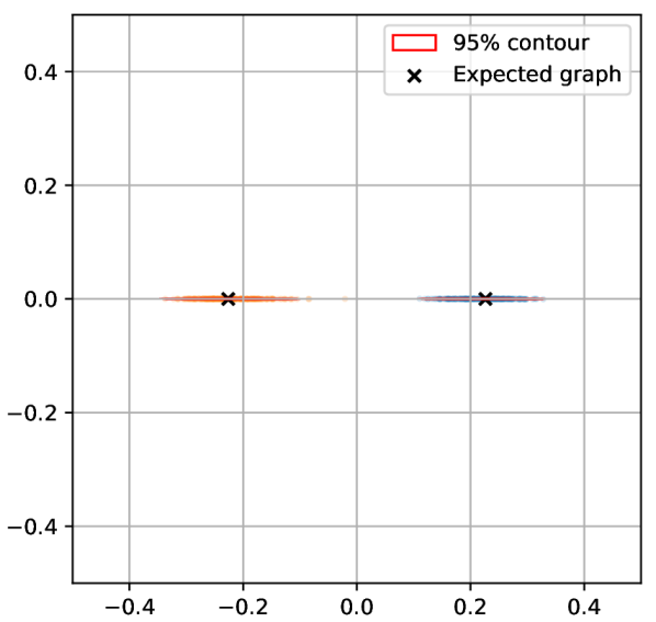
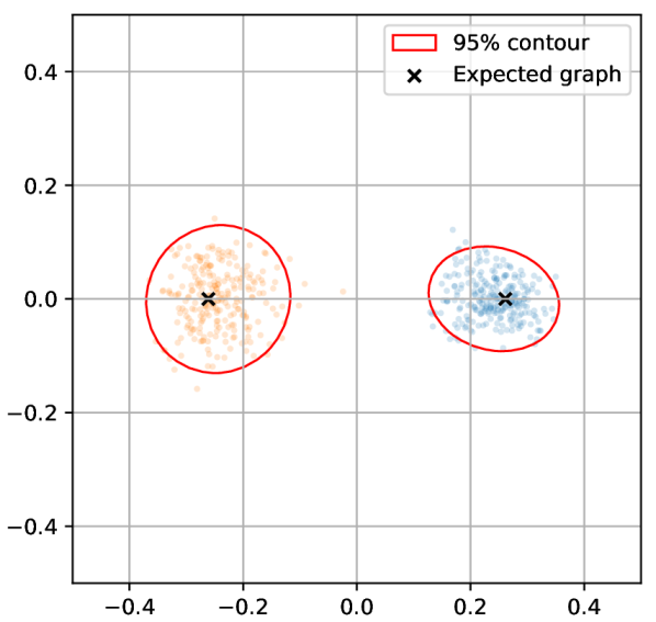
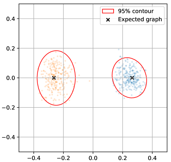
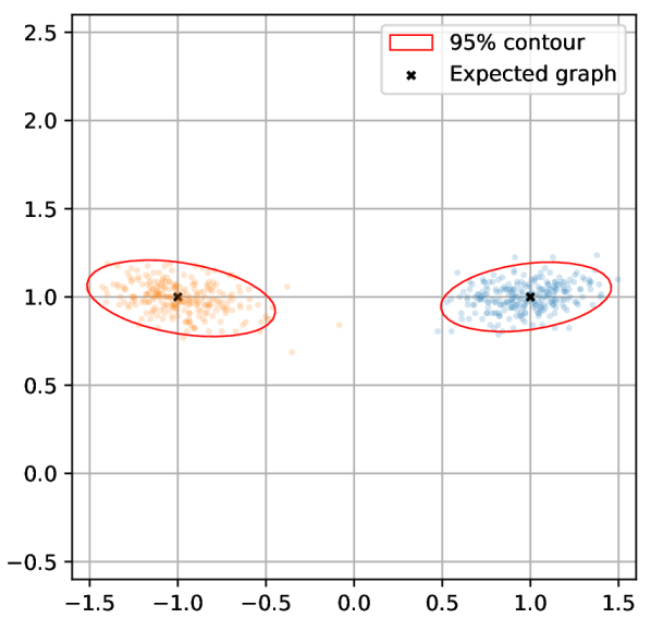
The geometry of node embedding vectors from SC, VEC, GramErgoPMI and ErgoVEC are shown in Fig. 2. We plot the 2D 95% confidence ellipse for each embedding cluster (red-colored elliptical curves) based on a maximum likelihood Gaussian fit to the data. For SC, ErgoVEC, and GramErgoPMI, the embeddings of the expected SBM graph are two distinct points (characterized in Theorem 3 and Corollary 1) which are marked as black crosses in Fig. 2. Since the VEC objective is based on empirical skip bigram counts from random walks, for a finite random walk length \ell, the embedding vectors of the expected graph will not collapse to two just distinct points, but will be distributed around the embedding vectors of ErgoVEC which are indicated as black crossses in the VEC subplot of Fig. 2.
Refer to caption
(a)      SC
Refer to caption
(b)      VEC
Refer to caption
(c)      ErgoPMI
Refer to caption
(d)      ErgoVEC
Figure 2: 2D-visualization of embeddings for SC, VEC, ErgoPMI and ErgoVEC. All four algorithms receive the same graph input with n=500𝑛500n=500 nodes generated using within community edge probabilities p=9lnn/n𝑝9𝑛𝑛p=9\ln{n}/n and across community edge probabilities q=2lnn/n𝑞2𝑛𝑛q=2\ln{n}/n.

In Fig. 2, we observe that in all four algorithms, the node embeddings in each cluster have an elliptical distribution around the cluster centroid and they can be perfectly separated linearly by the bisector of the line joining the two cluster centroids. However, the major axes of the SC embedding ellipses are nearly parallel to their inter-centroid line whereas the major axes of embedding ellipses in the other three algorithms are nearly perpendicular to their respective inter-centroid lines.

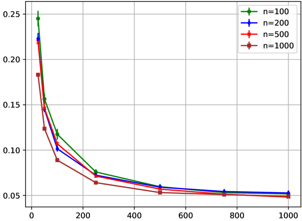
We also notice that the embedding ellipses of VEC and ErgoVEC in Fig. 2 look very similar. This is to be expected as the ErgoVEC objective is exactly the large \ell ergodic limit of the VEC objective introduced in Section 3.1. To empirically confirm that the ErgoVEC embeddings converge to the VEC embeddings in the large \ell limit, in Fig. 3 we plot the distance between VEC and ErgoVEC embeddings for increasing values of \ell and different graph sizes.

Refer to caption
Figure 3: Convergence of VEC embeddings: Frobenius norm distance between the Gram matrices of VEC and ErgoVEC versus random walk length \ell.

In order to measure the distance between embeddings up to any orthogonal transformation, we use the normalized Frobenius norm distance between the Gram matrices of the embeddings. For each n𝑛n, graphs are generated using within-community edge probabilities p=9lnn/n𝑝9𝑛𝑛p=9\ln{n}/n and across-community edge probabilities q=2lnn/n𝑞2𝑛𝑛q=2\ln{n}/n. The plot depicts the mean distance and associated error bar averaged over 555 independent graph realizations. Observe that for all graph sizes n=100,200,500,1000𝑛1002005001000n=100,200,500,1000, as the length of the random walk increases, the distance between VEC and ErgoVEC Gram matrices shrinks. However, due to the non-convexity of the VEC and and lack of global convergence guarantees for SGD methods used to optimize VEC and ErgoVEC objectives (cf. Section 4.2), the distance seems to be strictly bounded away from zero even at =10001000\ell=1000. However, the positive and negative w𝑤w-skip bigram counts and the objective function of VEC do converge to their respective ErgoVEC counterparts as \ell increases to infinity.

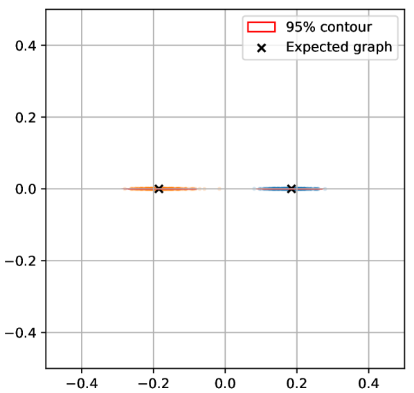
We now discuss the embedding geometry of NucGramErgoVEC. We separated this discussion from the previous four algorithms because although the embeddings of NucGramErgoVEC are also elliptically distributed and separate well into two clusters, the specific shape depends on the nuclear norm linear scaling factor ν0subscript𝜈0\nu_{0} as shown in Fig. 4.

Refer to caption
(a)      ν0=0.036subscript𝜈00.036\nu_{0}=0.036
Refer to caption
(b)      ν0=0.054subscript𝜈00.054\nu_{0}=0.054
Refer to caption
(c)      ν0=0.072subscript𝜈00.072\nu_{0}=0.072
Refer to caption
(d)      ν0=0.108subscript𝜈00.108\nu_{0}=0.108
Figure 4: 2D-visualization of NucGramErgoVEC embeddings for different nuclear norm linear scaling factors. The input graph is the same as the one used in Fig. 2.

When ν0subscript𝜈0\nu_{0} is very small, the embeddings are one dimensional (cf. Fig. 4(a)). As ν0subscript𝜈0\nu_{0} increases slightly, the embeddings remains one dimensional but spread out within each cluster and the cluster centroids move apart (cf. Fig. 4(b)). This continues until ν0subscript𝜈0\nu_{0} reaches a threshold. When ν0subscript𝜈0\nu_{0} increases beyond the threshold, the embeddings stop extending in the first dimension and start to spread in the second dimension (cf. Fig. 4(c)(d)).

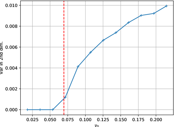
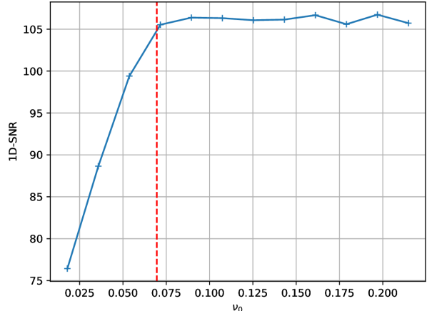
In order to obtain a more quantitative understanding of how ν0subscript𝜈0\nu_{0} influences the embedding geometry, we plot the 1D-SNR of embeddings and their variance in the second dimension for a range of values of ν0subscript𝜈0\nu_{0} in Fig. 5.

Refer to caption
(a) Variance in 2nd dim.
Refer to caption
(b) 1D-SNR
Figure 5: The change in (a) variance in second dimension and (b) 1D-SNR of NucGramErgoVEC embeddings as the nuclear norm linear scaling factor ν0subscript𝜈0\nu_{0} increases. The input graph has n=200𝑛200n=200 nodes generated with within community edge probabilities p=9lnn/n𝑝9𝑛𝑛p=9\ln{n}/n and across community edge probabilities q=2lnn/n𝑞2𝑛𝑛q=2\ln{n}/n.

Fig 5(a) shows how the variance of embeddings in the second dimension changes as the nuclear norm linear scaling factor ν0subscript𝜈0\nu_{0} increases. When ν0subscript𝜈0\nu_{0} is very small, the variance in the second dimension is 00, suggesting that embeddings are 111 dimensional. As ν0subscript𝜈0\nu_{0} increases, the variance in the second dimension remains zero until ν0subscript𝜈0\nu_{0} crosses a threshold that lies somewhere between ν0=0.054subscript𝜈00.054\nu_{0}=0.054 and ν0=0.072subscript𝜈00.072\nu_{0}=0.072 and then thereafter the variance increases monotonically. The exact value of ν0subscript𝜈0\nu_{0} where the second dimension variance emerges depends on the input graph in general and specifically on the edge forming probability.

Fig 5(b) shows how ν0subscript𝜈0\nu_{0} affects 1D-SNR of the embeddings. Here, we see a clear increase of 1D-SNR as ν0subscript𝜈0\nu_{0} increase from 0.0180.0180.018 to 0.0720.0720.072. A relative maximum level is reached when the ν0subscript𝜈0\nu_{0} is around the transition point where the second dimension variance emerges. Beyond the transition point, the 1D-SNR holds steady around the maximum level. These properties are consistent with our observations for Fig. 4.

5.2 Concentration of embeddings

After understanding how the geometry of embeddings of a single graph differs across embedding algorithms and changes with ν0subscript𝜈0\nu_{0}, in this section, we explore how the embeddings change as n𝑛n, the number of nodes, increases. To focus on the effect of increasing the number of nodes, throughout this section, we fix the scaling factors of edge forming probabilities within and across communities in each set of experiments. In addition, we omit the results of VEC because of their similarity to ErgoVEC (cf. Fig. 3). As we will see, the asymptotic behavior of embeddings largely depends on the edge forming probability.

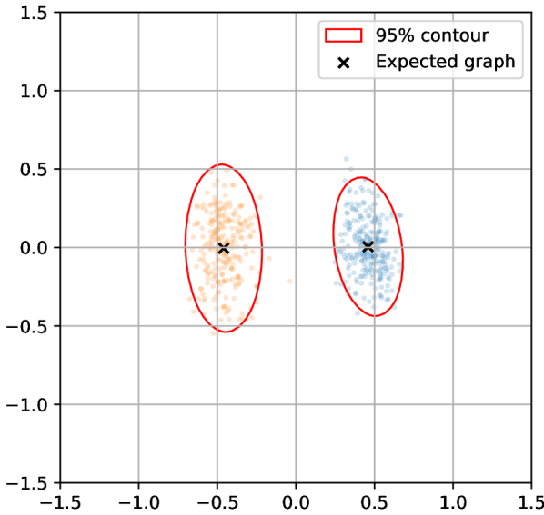
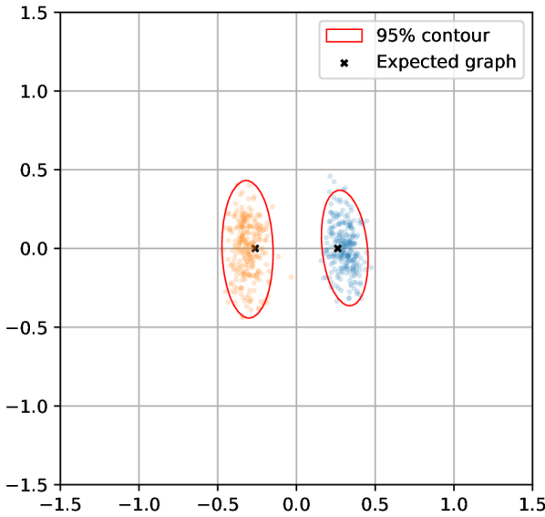
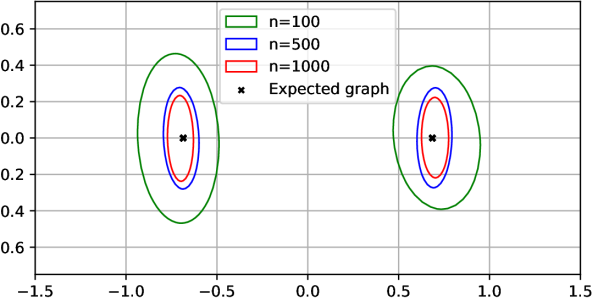
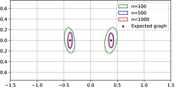
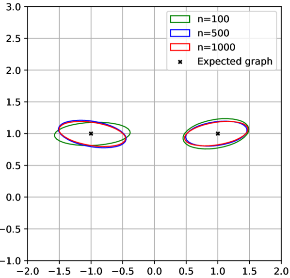
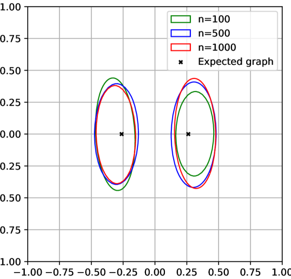
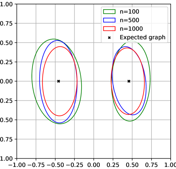
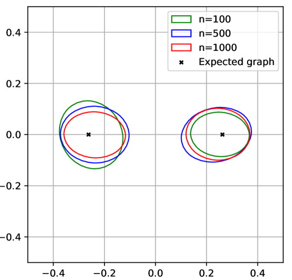
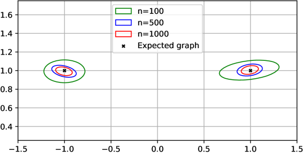
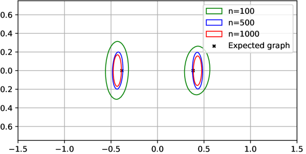
To gain a qualitative perspective, we first plot the embeddings and their 95%percent9595\% Gaussian contours for graph sizes n=100,500,1000𝑛1005001000n=100,500,1000 for each algorithm. Fig. 6 shows the embedding contours in the linear degree scaling regime. We can see that all the contours shrink as n𝑛n increases. This suggests that empirically, the embeddings of all the four algorithms concentrate to their centroids. In the logarithmic degree scaling regime, as shown in Fig. 7, the Gaussian contours for different graph sizes mostly overlap on top of each other, suggesting a convergence in distribution as opposed to a concentration that we observed in the linear regime.
Refer to caption
(a)   SC
Refer to caption
(b)   ErgoVEC
Refer to caption
(c)   ErgoPMI
   
Refer to caption
(d)   NucGramErgoVEC
ν0=0.108subscript𝜈00.108\nu_{0}=0.108
Figure 6: 95% Gaussian contours of 2D-embeddings from four algorithms in the linear regime. All algorithms receive the same sets of graphs with n=100,500𝑛100500n=100,500 and 100010001000 nodes generated using within-community edge probabilities p=0.6𝑝0.6p=0.6 and across community edge probabilities q=0.06𝑞0.06q=0.06.
Refer to caption
(a)     SC
Refer to caption
(b)     ErgoVEC
Refer to caption
(c)     ErgoPMI
   
Refer to caption
(d)   NucGramErgoVEC
ν0=0.108subscript𝜈00.108\nu_{0}=0.108
Figure 7: 95% Gaussian contours of 2D-embeddings from four algorithms in the logarithmic regime. All algorithms receive the same sets of graphs with n=100,500𝑛100500n=100,500 and 100010001000 nodes generated using within-community edge probabilities p=9lnn/n𝑝9𝑛𝑛p=9\ln{n}/n and across community edge probabilities q=2lnn/n𝑞2𝑛𝑛q=2\ln{n}/n.

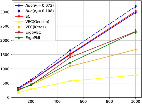
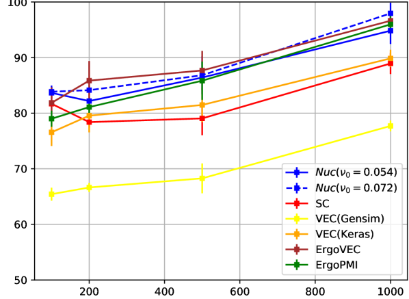
We turn to quantitative metrics to gain a more nuanced understanding. In Fig. 8, we plot the 1D-SNR of embeddings for increasing values of n𝑛n for each algorithm. Note that a higher 1D-SNR indicates either a smaller within group variance along the line that joins the cluster centroids or a greater distance between cluster centroids. Fig. 8(a) shows results for the linear degree scaling regime, where we see that 1D-SNR increases as n𝑛n increases, with NucGramErgoVEC leading, followed by SC, ErgoVEC and ErgoPMI. The VEC embeddings obtained from both implementations (Keras and Gensim) reside at the bottom. In the logarithmic degree scaling regime, as shown in Fig. 8(b), the 1D-SNR is relatively steady across different n𝑛n as opposed to a clear a growth trend observed in the linear degree scaling regime. This is consistent with our observations for Fig. 6 and Fig. 7 that the embeddings concentrate in linear regime but converges to a fixed distribution in the logarithmic regime. While VEC embeddings still under perform, ErgoPMI and ErgoVEC surpasses SC and catches NucGramErgoVEC’s lead.
Refer to caption
(a) Linear regime
Refer to caption
(b) Logarithmic regime
Figure 8: 1D-SNR versus graph size in the linear and logarithmic scaling regimes.

6 Concluding remarks

In this paper, we proposed a novel framework consisting of ergodic limits of random walks and a Grammian re-parameterization of the embedding objective to analyze a large class of random walk based node-embedding algorithms. In particular, we derived a closed-form expression for the ergodic limit of the random walk node embedding objective and proved that under the positive semi-definite constraint, the Gram matrix of optimum embedding vectors for two-community expected SBM graphs has either rank 111 or rank 222. In addition, through an empirical study we demonstrated that the embeddings based on ergodic limits, while forming better clusters, in terms of 1D-SNR, compared to the original random walk embeddings, concentrate to the embeddings of the expected graph in the linear degree scaling regime and seem to converge to a fixed distribution in the logarithmic regime.

Computational costs can vary substantially across different algorithms. For example, the Gram matrix of the optimal embedding vectors in ErgoPMI has a simple closed-form solution, whereas the better performing NucGramErgoVEC requires a computationally expensive iterative optimization procedure to compute the optimal Grammian. This suggests a possible trade-off between computational cost and accuracy of algorithms. Although not the focus of this paper, understanding these trade-offs would benefit the end users of these methods.

The results of this paper can be further improved and extended on both theoretical and practical fronts. For simplicity we focused on SBM graphs with two balanced communities. Our theoretical and experimental results can be potentially extended to more complex graph models that have a community structure. On the theoretical side, although we have shown perfect separation of the embeddings of the expected graph, there is no theoretical guarantee that the embeddings of SBM random graphs will concentrate to those of the expected graph. Further analysis of random walk embedding algorithms, especially the concentration properties of their solutions in various degree scaling regimes, would bring us more insight and understanding. On the practical side, the convergence of our Keras implementations for VEC and ErgoVEC depend highly on tuning parameters and may not converge very well, and the Hazan’s algorithm for NucGramErgoVEC suffers from slow convergence. Developing more scalable implementations of algorithms with faster and more stable convergence can bring these generalized formulations into large-scale real-world problems and also guide the theoretical analysis endeavor.

Appendix A

A.1 Proof of Theorem 1

Natural random walks will remain within the connected components in which they start. Since only pairs of nodes within the same connected component will occur in any random walk, we can analyze each connected component separately. Within each connected component 𝒢tsubscript𝒢𝑡\mathcal{G}_{t}, the random walk has transition matrix Wt=Dt1Atsubscript𝑊𝑡superscriptsubscript𝐷𝑡1subscript𝐴𝑡W_{t}=D_{t}^{-1}A_{t}. The proof of the theorem will follow immediately from the following lemma which focuses on connected graphs.

Lemma 1.

Let W𝑊W be the probability transition matrix of an irreducible Markov chain on the (finite) node space of 𝒢𝒢\mathcal{G}. Let the VEC algorithm be executed on 𝒢𝒢\mathcal{G} with random walk transition matrix W𝑊W and parameters w𝑤w and k𝑘k. Then for all i,j𝑖𝑗i,j, the ergodic limits n¯ij+superscriptsubscript¯𝑛𝑖𝑗\bar{n}_{ij}^{+} and n¯ijsuperscriptsubscript¯𝑛𝑖𝑗\bar{n}_{ij}^{-} in Definition 2 exist and are given by

n¯ij+=superscriptsubscript¯𝑛𝑖𝑗absent\displaystyle\bar{n}_{ij}^{+}={} πiv=1w(Wv)ij,subscript𝜋𝑖superscriptsubscript𝑣1𝑤subscriptsuperscript𝑊𝑣𝑖𝑗\displaystyle\pi_{i}\sum_{v=1}^{w}(W^{v})_{ij},
n¯ij=superscriptsubscript¯𝑛𝑖𝑗absent\displaystyle\bar{n}_{ij}^{-}={} kwπiπj,𝑘𝑤subscript𝜋𝑖subscript𝜋𝑗\displaystyle kw\pi_{i}\pi_{j},

where 𝛑𝛑\bm{\pi} is the unique stationary distribution of the random walk. Moreover, the Ergodic limiting coefficients are symmetric, i.e.,

n¯ij+=superscriptsubscript¯𝑛𝑖𝑗absent\displaystyle\bar{n}_{ij}^{+}={} n¯ji+,superscriptsubscript¯𝑛𝑗𝑖\displaystyle\bar{n}_{ji}^{+},
n¯ij=superscriptsubscript¯𝑛𝑖𝑗absent\displaystyle\bar{n}_{ij}^{-}={} n¯ji.superscriptsubscript¯𝑛𝑗𝑖\displaystyle\bar{n}_{ji}^{-}.

The proof of Lemma 1 is based on convergence results for irreducible Markov chains.

First, we prove the result for positive pairs. Let {Xs(m,p)}s=1superscriptsubscriptsuperscriptsubscript𝑋𝑠𝑚𝑝𝑠1\{X_{s}^{(m,p)}\}_{s=1}^{\infty} be the p𝑝p-th random walk starting from node m𝑚m following the transition matrix W𝑊W. We examine the first \ell steps in each random walk. Since the nij+superscriptsubscript𝑛𝑖𝑗n_{ij}^{+}’s consist of positive pairs extracted from all rn𝑟𝑛rn random walks (r𝑟r walks from each of the n𝑛n nodes), we have

nij+nr=1nrlm=1np=1rv=1ws=1v𝟏{Xs(m,p)=i,Xs+v(m,p)=j}.superscriptsubscript𝑛𝑖𝑗𝑛𝑟1𝑛𝑟𝑙superscriptsubscript𝑚1𝑛superscriptsubscript𝑝1𝑟superscriptsubscript𝑣1𝑤superscriptsubscript𝑠1𝑣subscript1formulae-sequencesuperscriptsubscript𝑋𝑠𝑚𝑝𝑖superscriptsubscript𝑋𝑠𝑣𝑚𝑝𝑗\frac{n_{ij}^{+}}{nr\ell}={}\frac{1}{nrl}\sum_{m=1}^{n}\sum_{p=1}^{r}\sum_{v=1}^{w}\sum_{s=1}^{\ell-v}\mathbf{1}_{\{X_{s}^{(m,p)}=i,X_{s+v}^{(m,p)}=j\}}. (21)

Letting \ell go to infinity on both sides, we have

1rnlimnij+1𝑟𝑛subscriptsuperscriptsubscript𝑛𝑖𝑗\displaystyle\frac{1}{rn}\lim_{\ell\rightarrow\infty}\frac{n_{ij}^{+}}{\ell}
=\displaystyle={} 1nrm=1np=1rv=1wlim1s=1v𝟏{Xs(m,p)=i,Xs+v(m,p)=j}.1𝑛𝑟superscriptsubscript𝑚1𝑛superscriptsubscript𝑝1𝑟superscriptsubscript𝑣1𝑤subscript1superscriptsubscript𝑠1𝑣subscript1formulae-sequencesuperscriptsubscript𝑋𝑠𝑚𝑝𝑖superscriptsubscript𝑋𝑠𝑣𝑚𝑝𝑗\displaystyle\frac{1}{nr}\sum_{m=1}^{n}\sum_{p=1}^{r}\sum_{v=1}^{w}\lim_{\ell\rightarrow\infty}\frac{1}{\ell}\sum_{s=1}^{\ell-v}\mathbf{1}_{\{X_{s}^{(m,p)}=i,X_{s+v}^{(m,p)}=j\}}.

The key step is to compute lim1s=1v𝟏{Xs(m,p)=i,Xs+v(m,p)=j}subscript1superscriptsubscript𝑠1𝑣subscript1formulae-sequencesuperscriptsubscript𝑋𝑠𝑚𝑝𝑖superscriptsubscript𝑋𝑠𝑣𝑚𝑝𝑗\lim\limits_{\ell\rightarrow\infty}\frac{1}{\ell}\sum_{s=1}^{\ell-v}\mathbf{1}_{\{X_{s}^{(m,p)}=i,X_{s+v}^{(m,p)}=j\}}. To begin, we define a new Markov Chain {Ys(m,p)}s=1superscriptsubscriptsuperscriptsubscript𝑌𝑠𝑚𝑝𝑠1\{Y_{s}^{(m,p)}\}_{s=1}^{\infty}, where Ys(m,p)=(Xs(m,p),Xs+1(m,p),,Xs+v(m,p))superscriptsubscript𝑌𝑠𝑚𝑝superscriptsubscript𝑋𝑠𝑚𝑝superscriptsubscript𝑋𝑠1𝑚𝑝superscriptsubscript𝑋𝑠𝑣𝑚𝑝Y_{s}^{(m,p)}\!=(X_{s}^{(m,p)}\!,X_{s+1}^{(m,p)}\!,\ldots,X_{s+v}^{(m,p)}). The state space of {Ys(m,p)}s=1superscriptsubscriptsuperscriptsubscript𝑌𝑠𝑚𝑝𝑠1\{Y_{s}^{(m,p)}\}_{s=1}^{\infty} is the set of all length-(v+1)𝑣1(v+1) walks under W𝑊W, i.e., Sv={(i1,i2,,iv+1)|ik+1 is accessible from ik,k=1,,v}[n]v+1subscript𝑆𝑣conditional-setsubscript𝑖1subscript𝑖2subscript𝑖𝑣1formulae-sequencesubscript𝑖𝑘1 is accessible from subscript𝑖𝑘𝑘1𝑣superscriptdelimited-[]𝑛𝑣1S_{v}=\{(i_{1},i_{2},\ldots,i_{v+1})\ \big{|}\ i_{k+1}\text{ is accessible from }i_{k},k=1,\ldots,v\}\subset{[n]^{v+1}}.

We claim that {Ys(m,p)}s=1superscriptsubscriptsuperscriptsubscript𝑌𝑠𝑚𝑝𝑠1\{Y_{s}^{(m,p)}\}_{s=1}^{\infty} is a positive recurrent Markov Chain. To see this, we first note that the state space is finite as |Sv||[n]v+1|=nv+1<subscript𝑆𝑣superscriptdelimited-[]𝑛𝑣1superscript𝑛𝑣1|S_{v}|\leq|[n]^{v+1}|=n^{v+1}<\infty. Then, we notice that 𝒂,𝒃Svfor-all𝒂𝒃subscript𝑆𝑣\forall\bm{a},\bm{b}\in S_{v}, since W𝑊W is irreducible, b1subscript𝑏1b_{1} is reachable from av+1subscript𝑎𝑣1a_{v+1} in Xs(m,p)superscriptsubscript𝑋𝑠𝑚𝑝X_{s}^{(m,p)}. Therefore, 𝒃𝒃\bm{b} is also reachable from 𝒂𝒂\bm{a}, which shows that Ys(m,p)superscriptsubscript𝑌𝑠𝑚𝑝Y_{s}^{(m,p)} is irreducible. An irreducible Markov chain on a finite state space must be positive recurrent.

Applying standard results from renewal theory, specifically [48, Proposition 3.3.1, p.102] to Markov chain {Xs(m,p)}s=1superscriptsubscriptsuperscriptsubscript𝑋𝑠𝑚𝑝𝑠1\{X_{s}^{(m,p)}\}_{s=1}^{\infty} and [48, Theorem 3.3.4, p.107] to Markov chain {Ys(m,p)}s=1superscriptsubscriptsuperscriptsubscript𝑌𝑠𝑚𝑝𝑠1\{Y_{s}^{(m,p)}\}_{s=1}^{\infty}, we get

lims=1𝟏{Xs(m,p)=i}=πi,a.s.,subscriptsuperscriptsubscript𝑠1subscript1superscriptsubscript𝑋𝑠𝑚𝑝𝑖subscript𝜋𝑖a.s.\displaystyle\lim_{\ell\rightarrow\infty}\frac{\sum_{s=1}^{\ell}\mathbf{1}_{\{X_{s}^{(m,p)}=i\}}}{\ell}=\pi_{i},\qquad\text{a.s.},
lim𝔼s=1𝟏{Xs(m,p)=i}=πi,subscript𝔼superscriptsubscript𝑠1subscript1superscriptsubscript𝑋𝑠𝑚𝑝𝑖subscript𝜋𝑖\displaystyle\lim_{\ell\rightarrow\infty}\frac{\mathbb{E}\sum_{s=1}^{\ell}\mathbf{1}_{\{X_{s}^{(m,p)}=i\}}}{\ell}=\pi_{i}, (22)
lims=1𝟏{Ys(m,p)=𝒂}=η𝒂,a.s.,subscriptsuperscriptsubscript𝑠1subscript1superscriptsubscript𝑌𝑠𝑚𝑝𝒂subscript𝜂𝒂a.s.\displaystyle\lim_{\ell\rightarrow\infty}\frac{\sum_{s=1}^{\ell}\mathbf{1}_{\{Y_{s}^{(m,p)}=\bm{a}\}}}{\ell}=\eta_{\bm{a}},\qquad\text{a.s.}, (23)
lim𝔼s=1𝟏{Ys(m,p)=𝒂}=η𝒂,subscript𝔼superscriptsubscript𝑠1subscript1superscriptsubscript𝑌𝑠𝑚𝑝𝒂subscript𝜂𝒂\displaystyle\lim_{\ell\rightarrow\infty}\frac{\mathbb{E}\sum_{s=1}^{\ell}\mathbf{1}_{\{Y_{s}^{(m,p)}=\bm{a}\}}}{\ell}=\eta_{\bm{a}},

where 𝝅𝝅\bm{\pi} and 𝜼𝜼\bm{\eta} are the stationary distributions of Xs(m,p)superscriptsubscript𝑋𝑠𝑚𝑝X_{s}^{(m,p)} and Ys(m,p)superscriptsubscript𝑌𝑠𝑚𝑝Y_{s}^{(m,p)}, respectively, and do not depend on m,p𝑚𝑝m,p because of the positive recurrence and irreducibility of the Markov chains. Note that the relationship between state counts of Xs(m,p)superscriptsubscript𝑋𝑠𝑚𝑝X_{s}^{(m,p)} and Ys(m,p)superscriptsubscript𝑌𝑠𝑚𝑝Y_{s}^{(m,p)} is given by

𝟏{Xs(m,p)=i,Xs+v(m,p)=j}=𝒂:a1=i,av+1=j𝟏{Ys(m,p)=𝒂}.subscript1formulae-sequencesuperscriptsubscript𝑋𝑠𝑚𝑝𝑖superscriptsubscript𝑋𝑠𝑣𝑚𝑝𝑗subscript:𝒂formulae-sequencesubscript𝑎1𝑖subscript𝑎𝑣1𝑗subscript1superscriptsubscript𝑌𝑠𝑚𝑝𝒂\mathbf{1}_{\{X_{s}^{(m,p)}=i,X_{s+v}^{(m,p)}=j\}}=\sum_{\bm{a}:\ a_{1}=i,a_{v+1}=j}\mathbf{1}_{\{Y_{s}^{(m,p)}=\bm{a}\}}.

And thus,

lim1s=1𝟏{Xs(m,p)=i,Xs+v(m,p)=j}subscript1superscriptsubscript𝑠1subscript1formulae-sequencesuperscriptsubscript𝑋𝑠𝑚𝑝𝑖superscriptsubscript𝑋𝑠𝑣𝑚𝑝𝑗\displaystyle\lim_{\ell\rightarrow\infty}\frac{1}{\ell}\sum_{s=1}^{\ell}\mathbf{1}_{\{X_{s}^{(m,p)}=i,X_{s+v}^{(m,p)}=j\}}
=\displaystyle={} lim1𝒂:a1=i,av+1=j𝟏{Ys(m,p)=𝒂}subscript1subscript:𝒂formulae-sequencesubscript𝑎1𝑖subscript𝑎𝑣1𝑗subscript1superscriptsubscript𝑌𝑠𝑚𝑝𝒂\displaystyle\lim_{\ell\rightarrow\infty}\frac{1}{\ell}\sum_{\bm{a}:\ a_{1}=i,a_{v+1}=j}\mathbf{1}_{\{Y_{s}^{(m,p)}=\bm{a}\}}
=(23)superscript(23)\displaystyle\stackrel{{\scriptstyle\mathclap{\mathrm{\eqref{Eq:Lemma1_proof_+Y_as}}}}}{{=}}{} 𝒂:a1=i,av+1=jη𝒂subscript:𝒂formulae-sequencesubscript𝑎1𝑖subscript𝑎𝑣1𝑗subscript𝜂𝒂\displaystyle\sum_{\bm{a}:\ a_{1}=i,a_{v+1}=j}\eta_{\bm{a}}
=\displaystyle={} 𝒂:a1=i,av+1=jlims[Ys(m,p)=𝐚]subscript:𝒂formulae-sequencesubscript𝑎1𝑖subscript𝑎𝑣1𝑗subscript𝑠delimited-[]superscriptsubscript𝑌𝑠𝑚𝑝𝐚\displaystyle\sum_{\bm{a}:\ a_{1}=i,a_{v+1}=j}\lim_{s\to\infty}\mathbb{P}[Y_{s}^{(m,p)}=\mathbf{a}]
=\displaystyle={} lims(Xs(m,p)=i,Xs+v(m,p)=j)subscript𝑠formulae-sequencesuperscriptsubscript𝑋𝑠𝑚𝑝𝑖superscriptsubscript𝑋𝑠𝑣𝑚𝑝𝑗\displaystyle\lim_{s\to\infty}\mathbb{P}(X_{s}^{(m,p)}=i,X_{s+v}^{(m,p)}=j)
=\displaystyle={} lims=1(Xs(m,p)=i,Xs+v(m,p)=j)subscriptsuperscriptsubscript𝑠1formulae-sequencesuperscriptsubscript𝑋𝑠𝑚𝑝𝑖superscriptsubscript𝑋𝑠𝑣𝑚𝑝𝑗\displaystyle\lim_{\ell\rightarrow\infty}\frac{\sum_{s=1}^{\ell}\mathbb{P}(X_{s}^{(m,p)}=i,X_{s+v}^{(m,p)}=j)}{\ell}
=\displaystyle={} (W)ijvlims=1(Xs(m,p)=i)subscriptsuperscript𝑊𝑣𝑖𝑗subscriptsuperscriptsubscript𝑠1superscriptsubscript𝑋𝑠𝑚𝑝𝑖\displaystyle(W)^{v}_{ij}\lim_{\ell\rightarrow\infty}\frac{\sum_{s=1}^{\ell}\mathbb{P}(X_{s}^{(m,p)}=i)}{\ell}
=\displaystyle={} (W)ijvlim𝔼s=1𝟏{Xs(m,p)=i}subscriptsuperscript𝑊𝑣𝑖𝑗subscript𝔼superscriptsubscript𝑠1subscript1superscriptsubscript𝑋𝑠𝑚𝑝𝑖\displaystyle(W)^{v}_{ij}\lim_{\ell\rightarrow\infty}\frac{\mathbb{E}\sum_{s=1}^{\ell}\mathbf{1}_{\{X_{s}^{(m,p)}=i\}}}{\ell}
=(22)superscript(22)\displaystyle\stackrel{{\scriptstyle\mathclap{\mathrm{\eqref{Eq:Lemma1_proof_+X_e}}}}}{{=}}{} (Wv)ijπi.subscriptsuperscript𝑊𝑣𝑖𝑗subscript𝜋𝑖\displaystyle\ (W^{v})_{ij}\pi_{i}.

Therefore, we have

lim1s=1𝟏{Xs(m,p)=i,Xs+v(m,p)=j}=(Wv)ijπi,subscript1superscriptsubscript𝑠1subscript1formulae-sequencesuperscriptsubscript𝑋𝑠𝑚𝑝𝑖superscriptsubscript𝑋𝑠𝑣𝑚𝑝𝑗subscriptsuperscript𝑊𝑣𝑖𝑗subscript𝜋𝑖\lim_{\ell\rightarrow\infty}\frac{1}{\ell}\sum_{s=1}^{\ell}\mathbf{1}_{\{X_{s}^{(m,p)}=i,X_{s+v}^{(m,p)}=j\}}=(W^{v})_{ij}\pi_{i},

and

1rnlimnij+=1nrm=1np=1rv=1w(Wv)ijπi=πiv=1w(Wv)ij.1𝑟𝑛subscriptsuperscriptsubscript𝑛𝑖𝑗1𝑛𝑟superscriptsubscript𝑚1𝑛superscriptsubscript𝑝1𝑟superscriptsubscript𝑣1𝑤subscriptsuperscript𝑊𝑣𝑖𝑗subscript𝜋𝑖subscript𝜋𝑖superscriptsubscript𝑣1𝑤subscriptsuperscript𝑊𝑣𝑖𝑗\frac{1}{rn}\lim_{\ell\rightarrow\infty}\frac{n_{ij}^{+}}{\ell}=\frac{1}{nr}\sum_{m=1}^{n}\sum_{p=1}^{r}\sum_{v=1}^{w}(W^{v})_{ij}\pi_{i}=\pi_{i}\sum_{v=1}^{w}(W^{v})_{ij}.

We now analyize the ergodic limits of negative pairs. We first count the number of (i,j)𝑖𝑗(i,j) pairs in the negative multi-set.

Let Zc(m,p,v,s)superscriptsubscript𝑍𝑐𝑚𝑝𝑣𝑠Z_{c}^{(m,p,v,s)} be the second node in c𝑐c-th negative pair generated from the positive pair (Xs(m,p),Xs+v(m,p))superscriptsubscript𝑋𝑠𝑚𝑝superscriptsubscript𝑋𝑠𝑣𝑚𝑝(X_{s}^{(m,p)},X_{s+v}^{(m,p)}) (for each positive pair we generate k𝑘k negative pairs). Since all negative pairs are generated in an i.i.d. manner, for all m,p,v,s,c𝑚𝑝𝑣𝑠𝑐m,p,v,s,c, Zc(m,p,v,s),c=1,,kformulae-sequencesuperscriptsubscript𝑍𝑐𝑚𝑝𝑣𝑠𝑐1𝑘Z_{c}^{(m,p,v,s)},c=1,\ldots,k are i.i.d. random variables with a distribution specified by the unigram node frequencies computed from the collection of random walks X=m=1np=1r{X(m,p)}𝑋superscriptsubscript𝑚1𝑛superscriptsubscript𝑝1𝑟superscript𝑋𝑚𝑝X=\bigcup_{m=1}^{n}\bigcup_{p=1}^{r}\{X^{(m,p)}\}. As in Equation 21, the counts of negative pairs is given by

nijnr=1nrm=1np=1rv=1ws=1v𝟏{Xs(m,p)=i}c=1k𝟏{Zc(m,p,s,v)=j}.superscriptsubscript𝑛𝑖𝑗𝑛𝑟1𝑛𝑟superscriptsubscript𝑚1𝑛superscriptsubscript𝑝1𝑟superscriptsubscript𝑣1𝑤superscriptsubscript𝑠1𝑣subscript1superscriptsubscript𝑋𝑠𝑚𝑝𝑖superscriptsubscript𝑐1𝑘subscript1superscriptsubscript𝑍𝑐𝑚𝑝𝑠𝑣𝑗\frac{n_{ij}^{-}}{nr\ell}={}\frac{1}{nr\ell}\sum_{m=1}^{n}\sum_{p=1}^{r}\sum_{v=1}^{w}\sum_{s=1}^{\ell-v}\mathbf{1}_{\{X_{s}^{(m,p)}=i\}}\sum_{c=1}^{k}\mathbf{1}_{\{Z_{c}^{(m,p,s,v)}=j\}}. (24)

Letting \ell go to infinity on both sides, we get

1nrlimnij1𝑛𝑟subscriptsuperscriptsubscript𝑛𝑖𝑗\displaystyle\frac{1}{nr}\lim_{\ell\rightarrow\infty}\frac{n_{ij}^{-}}{\ell}
=\displaystyle={} v=1wc=1klim1nrm=1np=1rs=1v𝟏{Xs(m,p)=i}𝟏{Zc(m,p,s,v)=j}.superscriptsubscript𝑣1𝑤superscriptsubscript𝑐1𝑘subscript1𝑛𝑟superscriptsubscript𝑚1𝑛superscriptsubscript𝑝1𝑟superscriptsubscript𝑠1𝑣subscript1superscriptsubscript𝑋𝑠𝑚𝑝𝑖subscript1superscriptsubscript𝑍𝑐𝑚𝑝𝑠𝑣𝑗\displaystyle\!\!\!\sum_{v=1}^{w}\sum_{c=1}^{k}\lim_{\ell\rightarrow\infty}\frac{1}{nr\ell}\sum_{m=1}^{n}\sum_{p=1}^{r}\sum_{s=1}^{\ell-v}\mathbf{1}_{\{X_{s}^{(m,p)}=i\}}\mathbf{1}_{\{Z_{c}^{(m,p,s,v)}=j\}}. (25)

The remainder of the proof will focus on calculating the right hand side. For this purpose, we introduce the following proposition:

Notation: [n]:={1,,n}assigndelimited-[]𝑛1𝑛[n]\vcentcolon=\{1,\ldots,n\} and X[n]:=X1,,Xnassignsubscript𝑋delimited-[]𝑛subscript𝑋1subscript𝑋𝑛X_{[n]}\vcentcolon=X_{1},\ldots,X_{n}.

Proposition A.1.1.

Let {X,}subscript𝑋\{X_{\ell},\ell\in\mathbb{N}\} be a sequence of random variables with X[n]subscript𝑋delimited-[]𝑛X_{\ell}\in[n] for every \ell. Let φ:[n][0,1]:𝜑delimited-[]𝑛01\varphi:[n]\rightarrow[0,1]. For every L𝐿L\in\mathbb{N}, let q^L:[n]L[0,1]:subscript^𝑞𝐿superscriptdelimited-[]𝑛𝐿01\widehat{q}_{L}:[n]^{L}\rightarrow[0,1] and V[L](L){0,1}subscriptsuperscript𝑉𝐿delimited-[]𝐿01V^{(L)}_{[L]}\in\{0,1\} be a sequence of random variables such that

V[L](L)|X[L]i.i.dBer(q^L(X[L])),conditionalsubscriptsuperscript𝑉𝐿delimited-[]𝐿subscript𝑋delimited-[]𝐿i.i.dsimilar-toBersubscript^𝑞𝐿subscript𝑋delimited-[]𝐿V^{(L)}_{[L]}\ |\ X_{[L]}\overset{\text{i.i.d}}{\sim}\text{Ber}\left(\widehat{q}_{L}(X_{[L]})\right),

If for some p,q[0,1]𝑝𝑞01p,q\in[0,1],

1L=1Lφ(X)La.s.p,\frac{1}{L}\sum_{\ell=1}^{L}\varphi(X_{\ell})\xrightarrow[L\to\infty]{a.s.}p, (26)

and

q^L(X[L])La.s.q\widehat{q}_{L}(X_{[L]})\xrightarrow[L\to\infty]{a.s.}q (27)

then

1L=1Lφ(X)V(L)La.s.pq.\frac{1}{L}\sum_{\ell=1}^{L}\varphi(X_{\ell})V_{\ell}^{(L)}\xrightarrow[L\to\infty]{a.s.}pq.
Proof.
1L=1Lφ(X)V(L)=1𝐿superscriptsubscript1𝐿𝜑subscript𝑋superscriptsubscript𝑉𝐿absent\displaystyle\frac{1}{L}\sum_{\ell=1}^{L}\varphi(X_{\ell})V_{\ell}^{(L)}={} (1L=1Lφ(X)V(L)1L=1Lφ(X)q^L)1𝐿superscriptsubscript1𝐿𝜑subscript𝑋superscriptsubscript𝑉𝐿1𝐿superscriptsubscript1𝐿𝜑subscript𝑋subscript^𝑞𝐿\displaystyle\left(\frac{1}{L}\sum_{\ell=1}^{L}\varphi(X_{\ell})V_{\ell}^{(L)}-\frac{1}{L}\sum_{\ell=1}^{L}\varphi(X_{\ell})\widehat{q}_{L}\right)
+q^L1L=1Lφ(X).subscript^𝑞𝐿1𝐿superscriptsubscript1𝐿𝜑subscript𝑋\displaystyle\quad+\widehat{q}_{L}\frac{1}{L}\sum_{\ell=1}^{L}\varphi(X_{\ell}).

Due to Equations 26 and 27 we immediately have

q^L(1L=1Lφ(X))La.s.pq.\widehat{q}_{L}\left(\frac{1}{L}\sum_{\ell=1}^{L}\varphi(X_{\ell})\right)\xrightarrow[L\to\infty]{a.s.}pq.

We will prove that

1L=1Lφ(X)V(L)1L=1Lφ(X)q^La.s.0.\frac{1}{L}\sum_{\ell=1}^{L}\varphi(X_{\ell})V_{\ell}^{(L)}-\frac{1}{L}\sum_{\ell=1}^{L}\varphi(X_{\ell})\widehat{q}_{\ell}\xrightarrow[L\to\infty]{a.s.}0.

For any fixed x[L][n]subscript𝑥delimited-[]𝐿delimited-[]𝑛x_{[L]}\in[n], define g:[0,1]L[0,1]:𝑔superscript01𝐿01g:[0,1]^{L}\rightarrow[0,1] as

g(v[L]):=1L=1Lφ(x)v.assign𝑔subscript𝑣delimited-[]𝐿1𝐿superscriptsubscript1𝐿𝜑subscript𝑥subscript𝑣g(v_{[L]})\vcentcolon={}\frac{1}{L}\sum_{\ell=1}^{L}\varphi(x_{\ell})v_{\ell}.

We can show that g()𝑔g(\cdot) satisfies the so-called coordinate-wise bounded difference property. In fact, for any i[L]𝑖delimited-[]𝐿i\in[L] and any v[L],vi[0,1]subscript𝑣delimited-[]𝐿superscriptsubscript𝑣𝑖01v_{[L]},v_{i}^{\prime}\in[0,1], since φ(x)[0,1]𝜑𝑥01\varphi(x)\in[0,1], we have

|g(v[L])g(v[L]{i},vi)|𝑔subscript𝑣delimited-[]𝐿𝑔subscript𝑣delimited-[]𝐿𝑖superscriptsubscript𝑣𝑖\displaystyle\left|g(v_{[L]})-g(v_{[L]\setminus\{i\}},v_{i}^{\prime})\right|
=\displaystyle={} 1L|φ(xi)||(vivi)|1𝐿𝜑subscript𝑥𝑖subscript𝑣𝑖superscriptsubscript𝑣𝑖\displaystyle\frac{1}{L}\left|\varphi(x_{i})\right|\left|(v_{i}-v_{i}^{\prime})\right|
\displaystyle\leq{} 1L.1𝐿\displaystyle\frac{1}{L}.

Since , V[L](L)superscriptsubscript𝑉delimited-[]𝐿𝐿V_{[L]}^{(L)} are i.i.d. conditioned on X[L]subscript𝑋delimited-[]𝐿X_{[L]} and g()𝑔g(\cdot) is coordinate-wise bounded, we can apply McDiarmid’s inequality [49] to V[L](L)superscriptsubscript𝑉delimited-[]𝐿𝐿V_{[L]}^{(L)} and g()𝑔g(\cdot) under the conditional probability measure: ε>0for-all𝜀0\forall\varepsilon>0,

[|g(V[L](L))𝔼[g(V[L](L))|X[L]]|ε|X[L]]2e2Lε2.\mathbb{P}\left[\left|g(V_{[L]}^{(L)})-\mathbb{E}\left[g(V_{[L]}^{(L)})\Big{|}X_{[L]}\right]\right|\geq\varepsilon\Bigg{|}X_{[L]}\right]\leq{}2e^{-2L\varepsilon^{2}}.

Since the right hand side is constant and independent of X[L]subscript𝑋delimited-[]𝐿X_{[L]}, the above bound also holds for unconditional probability:

[|g(V[L](L))𝔼[g(V[L](L))|X[L]]|ε]2e2Lε2.\mathbb{P}\left[\left|g(V_{[L]}^{(L)})-\mathbb{E}\left[g(V_{[L]}^{(L)})\Big{|}X_{[L]}\right]\right|\geq\varepsilon\right]\leq{}2e^{-2L\varepsilon^{2}}.

Since

g(V[L](L))=1L=1Lφ(X)V(L),𝑔superscriptsubscript𝑉delimited-[]𝐿𝐿1𝐿superscriptsubscript1𝐿𝜑subscript𝑋superscriptsubscript𝑉𝐿g(V_{[L]}^{(L)})={}\frac{1}{L}\sum_{\ell=1}^{L}\varphi(X_{\ell})V_{\ell}^{(L)},

we have

𝔼[g(V[L](L))|X[L]]𝔼delimited-[]conditional𝑔superscriptsubscript𝑉delimited-[]𝐿𝐿subscript𝑋delimited-[]𝐿\displaystyle\mathbb{E}\left[g(V_{[L]}^{(L)})\Big{|}X_{[L]}\right] =𝔼[1L=1Lφ(X)V(L)|X[L]]absent𝔼delimited-[]conditional1𝐿superscriptsubscript1𝐿𝜑subscript𝑋superscriptsubscript𝑉𝐿subscript𝑋delimited-[]𝐿\displaystyle={}\mathbb{E}\left[\frac{1}{L}\sum_{\ell=1}^{L}\varphi(X_{\ell})V_{\ell}^{(L)}\Big{|}X_{[L]}\right]
=1L=1Lφ(X)𝔼[V(L)|X[L]]absent1𝐿superscriptsubscript1𝐿𝜑subscript𝑋𝔼delimited-[]conditionalsuperscriptsubscript𝑉𝐿subscript𝑋delimited-[]𝐿\displaystyle={}\frac{1}{L}\sum_{\ell=1}^{L}\varphi(X_{\ell})\mathbb{E}\left[V_{\ell}^{(L)}\Big{|}X_{[L]}\right]
=1L=1Lφ(X)q^.absent1𝐿superscriptsubscript1𝐿𝜑subscript𝑋subscript^𝑞\displaystyle={}\frac{1}{L}\sum_{\ell=1}^{L}\varphi(X_{\ell})\widehat{q}_{\ell}.

In other words, we have shown

[|1L=1Lφ(X)V(L)1L=1Lφ(X)q^|ε]2e2Lε2.delimited-[]1𝐿superscriptsubscript1𝐿𝜑subscript𝑋superscriptsubscript𝑉𝐿1𝐿superscriptsubscript1𝐿𝜑subscript𝑋subscript^𝑞𝜀2superscript𝑒2𝐿superscript𝜀2\mathbb{P}\left[\left|\frac{1}{L}\sum_{\ell=1}^{L}\varphi(X_{\ell})V_{\ell}^{(L)}-\frac{1}{L}\sum_{\ell=1}^{L}\varphi(X_{\ell})\widehat{q}_{\ell}\right|\geq\varepsilon\right]\leq{}2e^{-2L\varepsilon^{2}}.

Therefore,

L=1[|1L=1Lφ(X)V(L)1L=1Lφ(X)q^|ε]superscriptsubscript𝐿1delimited-[]1𝐿superscriptsubscript1𝐿𝜑subscript𝑋superscriptsubscript𝑉𝐿1𝐿superscriptsubscript1𝐿𝜑subscript𝑋subscript^𝑞𝜀\displaystyle\sum_{L=1}^{\infty}\mathbb{P}\left[\left|\frac{1}{L}\sum_{\ell=1}^{L}\varphi(X_{\ell})V_{\ell}^{(L)}-\frac{1}{L}\sum_{\ell=1}^{L}\varphi(X_{\ell})\widehat{q}_{\ell}\right|\geq\varepsilon\right]
\displaystyle\leq{} L=12e2Lε2superscriptsubscript𝐿12superscript𝑒2𝐿superscript𝜀2\displaystyle\sum_{L=1}^{\infty}2e^{-2L\varepsilon^{2}}
=\displaystyle={} 2e2ε21e2ε22superscript𝑒2superscript𝜀21superscript𝑒2superscript𝜀2\displaystyle\frac{2e^{-2\varepsilon^{2}}}{1-e^{-2\varepsilon^{2}}}
<\displaystyle<{} \displaystyle\infty

which proves that 1L=1Lφ(X)V(L)1L=1Lφ(X)q^1𝐿superscriptsubscript1𝐿𝜑subscript𝑋superscriptsubscript𝑉𝐿1𝐿superscriptsubscript1𝐿𝜑subscript𝑋subscript^𝑞\frac{1}{L}\sum_{\ell=1}^{L}\varphi(X_{\ell})V_{\ell}^{(L)}-\frac{1}{L}\sum_{\ell=1}^{L}\varphi(X_{\ell})\widehat{q}_{\ell} is converges to zero completely. Since complete convergence implies almost sure convergence [50, Theorem 4 (c),p.310], it follows that

1L=1Lφ(X)V(L)1L=1Lφ(X)q^La.s.0,\frac{1}{L}\sum_{\ell=1}^{L}\varphi(X_{\ell})V_{\ell}^{(L)}-\frac{1}{L}\sum_{\ell=1}^{L}\varphi(X_{\ell})\widehat{q}_{\ell}\xrightarrow[L\to\infty]{a.s.}0,

which completes the proof of this proposition. ∎

To compute the right hand side of Equation 25, for each fixed c,v𝑐𝑣c,v, we apply Proposition A.1.1 in the following way:

Identifying variables: Let Γ:={1,,n}×{1,,r}×{1,,}assignΓ1𝑛1𝑟1\Gamma\vcentcolon={}\{1,\dotsc,n\}\times\{1,\dotsc,r\}\times\{1,\dotsc,\ell\}. For γ=(m,p,s)𝛾𝑚𝑝𝑠\gamma={}(m,p,s), we define

L𝐿\displaystyle L :=|Γ|=nr,assignabsentΓ𝑛𝑟\displaystyle\vcentcolon={}|\Gamma|={}nr\ell,
Xγsubscript𝑋𝛾\displaystyle X_{\gamma} :=Xs(m,p)assignabsentsuperscriptsubscript𝑋𝑠𝑚𝑝\displaystyle\vcentcolon={}X_{s}^{(m,p)}
Vγ(L)superscriptsubscript𝑉𝛾𝐿\displaystyle V_{\gamma}^{(L)} :=𝟏{Zc(m,p,s,v)=j}assignabsentsubscript1superscriptsubscript𝑍𝑐𝑚𝑝𝑠𝑣𝑗\displaystyle\vcentcolon={}\mathbf{1}_{\{Z_{c}^{(m,p,s,v)}=j\}}
φ(Xγ)𝜑subscript𝑋𝛾\displaystyle\varphi(X_{\gamma}) :=𝟏{Xγ=i}assignabsentsubscript1subscript𝑋𝛾𝑖\displaystyle\vcentcolon={}\mathbf{1}_{\{X_{\gamma}=i\}}
q^L(X[L])subscript^𝑞𝐿subscript𝑋delimited-[]𝐿\displaystyle\widehat{q}_{L}(X_{[L]}) :=1LγΓ𝟏{Xγ=j}.assignabsent1𝐿subscript𝛾Γsubscript1subscript𝑋𝛾𝑗\displaystyle\vcentcolon={}\frac{1}{L}\sum_{\gamma\in\Gamma}\mathbf{1}_{\{X_{\gamma}=j\}}.

Verification of assumptions:

V[L](L)|X[L]conditionalsuperscriptsubscript𝑉delimited-[]𝐿𝐿subscript𝑋delimited-[]𝐿\displaystyle V_{[L]}^{(L)}\ \Big{|}\ X_{[L]} i.i.dBer(q^L(XL)),i.i.dsimilar-toBersubscript^𝑞𝐿subscript𝑋𝐿\displaystyle\overset{\text{i.i.d}}{\sim}\text{Ber}\left(\widehat{q}_{L}(X_{L})\right),
1LγΓφ(Xγ)1𝐿subscript𝛾Γ𝜑subscript𝑋𝛾\displaystyle\frac{1}{L}\sum_{\gamma\in\Gamma}\varphi(X_{\gamma}) La.s.πi,\displaystyle\xrightarrow[L\to\infty]{a.s.}\pi_{i},
q^L(X[L])=subscript^𝑞𝐿subscript𝑋delimited-[]𝐿absent\displaystyle\widehat{q}_{L}(X_{[L]})={} La.s.πj\displaystyle\xrightarrow[L\to\infty]{a.s.}\pi_{j}

Therefore, by Equation 25, we have

1LγΓφ(Xγ)V[L](L)a.s.πiπj.\frac{1}{L}\sum_{\gamma\in\Gamma}\varphi(X_{\gamma})V_{[L]}^{(L)}\xrightarrow[\ell\to\infty]{a.s.}\pi_{i}\pi_{j}.

Or equivalently, for each c,v𝑐𝑣c,v,

1nrm=1np=1rs=1𝟏{Xs(m,p)=i}𝟏{Zc(m,p,s,v)=j}a.s.πiπj.\frac{1}{nr\ell}\sum_{m=1}^{n}\sum_{p=1}^{r}\sum_{s=1}^{\ell}\mathbf{1}_{\{X_{s}^{(m,p)}=i\}}\mathbf{1}_{\{Z_{c}^{(m,p,s,v)}=j\}}\xrightarrow[\ell\to\infty]{a.s.}\pi_{i}\pi_{j}.

Dropping a finite number of terms in the summation will not affect the limit as \ell\rightarrow\infty. Thus,

1nrm=1np=1rs=1v𝟏{Xs(m,p)=i}𝟏{Zc(m,p,s,v)=j}a.s.πiπj.\frac{1}{nr\ell}\sum_{m=1}^{n}\sum_{p=1}^{r}\sum_{s=1}^{\ell-v}\mathbf{1}_{\{X_{s}^{(m,p)}=i\}}\mathbf{1}_{\{Z_{c}^{(m,p,s,v)}=j\}}\xrightarrow[\ell\to\infty]{a.s.}\pi_{i}\pi_{j}.

Together with Equation 25, we have

1nrlimnij1𝑛𝑟subscriptsuperscriptsubscript𝑛𝑖𝑗\displaystyle\frac{1}{nr}\lim_{\ell\rightarrow\infty}\frac{n_{ij}^{-}}{\ell}
=\displaystyle={} v=1wc=1klim1nrm=1np=1rs=1v𝟏{Xs(m,p)=i}𝟏{Zc(m,p,s,v)=j}superscriptsubscript𝑣1𝑤superscriptsubscript𝑐1𝑘subscript1𝑛𝑟superscriptsubscript𝑚1𝑛superscriptsubscript𝑝1𝑟superscriptsubscript𝑠1𝑣subscript1superscriptsubscript𝑋𝑠𝑚𝑝𝑖subscript1superscriptsubscript𝑍𝑐𝑚𝑝𝑠𝑣𝑗\displaystyle\sum_{v=1}^{w}\sum_{c=1}^{k}\lim_{\ell\rightarrow\infty}\frac{1}{nr\ell}\sum_{m=1}^{n}\sum_{p=1}^{r}\sum_{s=1}^{\ell-v}\mathbf{1}_{\{X_{s}^{(m,p)}=i\}}\mathbf{1}_{\{Z_{c}^{(m,p,s,v)}=j\}}
=\displaystyle={} v=1wc=1kπiπja.s.superscriptsubscript𝑣1𝑤superscriptsubscript𝑐1𝑘subscript𝜋𝑖subscript𝜋𝑗a.s.\displaystyle\sum_{v=1}^{w}\sum_{c=1}^{k}\pi_{i}\pi_{j}\qquad\text{a.s.}
=\displaystyle={} kwπiπj.a.s.\displaystyle kw\pi_{i}\pi_{j}.\quad\ \ \ \qquad\text{a.s.}

This concludes the proof of expressions for n¯ij+superscriptsubscript¯𝑛𝑖𝑗\bar{n}_{ij}^{+} and n¯ijsuperscriptsubscript¯𝑛𝑖𝑗\bar{n}_{ij}^{-} in Lemma 1 and also shows that n¯ij=n¯jisuperscriptsubscript¯𝑛𝑖𝑗superscriptsubscript¯𝑛𝑗𝑖\bar{n}_{ij}^{-}=\bar{n}_{ji}^{-} . In order to show that n¯ij+superscriptsubscript¯𝑛𝑖𝑗\bar{n}_{ij}^{+} is symmetric, it suffices to show that for any v𝑣v,

πi(Wv)ij=πj(Wv)ji.subscript𝜋𝑖subscriptsuperscript𝑊𝑣𝑖𝑗subscript𝜋𝑗subscriptsuperscript𝑊𝑣𝑗𝑖\pi_{i}(W^{v})_{ij}=\pi_{j}(W^{v})_{ji}.

Since πisubscript𝜋𝑖\pi_{i} is proportional to the node degree, this is equivalent to showing that

di(Wv)ij=dj(Wv)jisubscript𝑑𝑖subscriptsuperscript𝑊𝑣𝑖𝑗subscript𝑑𝑗subscriptsuperscript𝑊𝑣𝑗𝑖d_{i}(W^{v})_{ij}=d_{j}(W^{v})_{ji}

We will prove this via induction. For v=1𝑣1v=1, by definition, diWij=Aij=djWjisubscript𝑑𝑖subscript𝑊𝑖𝑗subscript𝐴𝑖𝑗subscript𝑑𝑗subscript𝑊𝑗𝑖d_{i}W_{ij}={}A_{ij}={}d_{j}W_{ji} (initial case). If di(Ws)ij=dj(Ws)jisubscript𝑑𝑖subscriptsuperscript𝑊𝑠𝑖𝑗subscript𝑑𝑗subscriptsuperscript𝑊𝑠𝑗𝑖d_{i}(W^{s})_{ij}={}d_{j}(W^{s})_{ji}, for v=s+1𝑣𝑠1v=s+1 (induction hypothesis), then

di(Ws+1)ij=subscript𝑑𝑖subscriptsuperscript𝑊𝑠1𝑖𝑗absent\displaystyle d_{i}(W^{s+1})_{ij}= k=1ndi(Ws)ikWkjsuperscriptsubscript𝑘1𝑛subscript𝑑𝑖subscriptsuperscript𝑊𝑠𝑖𝑘subscript𝑊𝑘𝑗\displaystyle\sum_{k=1}^{n}d_{i}(W^{s})_{ik}W_{kj}
=\displaystyle= k=1ndk(Ws)kiWkjsuperscriptsubscript𝑘1𝑛subscript𝑑𝑘subscriptsuperscript𝑊𝑠𝑘𝑖subscript𝑊𝑘𝑗\displaystyle\sum_{k=1}^{n}d_{k}(W^{s})_{ki}W_{kj}
=\displaystyle= k=1ndkWkj(Ws)kisuperscriptsubscript𝑘1𝑛subscript𝑑𝑘subscript𝑊𝑘𝑗subscriptsuperscript𝑊𝑠𝑘𝑖\displaystyle\sum_{k=1}^{n}d_{k}W_{kj}(W^{s})_{ki}
=\displaystyle= k=1ndjWjk(Ws)kisuperscriptsubscript𝑘1𝑛subscript𝑑𝑗subscript𝑊𝑗𝑘subscriptsuperscript𝑊𝑠𝑘𝑖\displaystyle\sum_{k=1}^{n}d_{j}W_{jk}(W^{s})_{ki}
=\displaystyle= dj(Ws+1)ji.subscript𝑑𝑗subscriptsuperscript𝑊𝑠1𝑗𝑖\displaystyle d_{j}(W^{s+1})_{ji}.

which proves the inductive step and concludes the proof of symmetry of n¯ij+superscriptsubscript¯𝑛𝑖𝑗\bar{n}_{ij}^{+}. \hfill\square

A.2 Proof of Theorem 2

We will follow the same ideas as in the proof of Lemma 1. With walk-distance weights {αv}v=1superscriptsubscriptsubscript𝛼𝑣𝑣1\{\alpha_{v}\}_{v=1}^{\infty}, the positive pair count Equation 21 becomes:

nij+nr=1nrlm=1np=1rv=1αvs=1v𝟏{Xs(m,p)=i,Xs+v(m,p)=j}.superscriptsubscript𝑛𝑖𝑗𝑛𝑟1𝑛𝑟𝑙superscriptsubscript𝑚1𝑛superscriptsubscript𝑝1𝑟superscriptsubscript𝑣1subscript𝛼𝑣superscriptsubscript𝑠1𝑣subscript1formulae-sequencesuperscriptsubscript𝑋𝑠𝑚𝑝𝑖superscriptsubscript𝑋𝑠𝑣𝑚𝑝𝑗\frac{n_{ij}^{+}}{nr\ell}={}\frac{1}{nrl}\sum_{m=1}^{n}\sum_{p=1}^{r}\sum_{v=1}^{\infty}\alpha_{v}\sum_{s=1}^{\ell-v}\mathbf{1}_{\{X_{s}^{(m,p)}=i,X_{s+v}^{(m,p)}=j\}}. (28)

And the negative pair count Equation 24 becomes:

nijnr=1nrm=1np=1rv=1αvs=1v𝟏{Xs(m,p)=i}c=1k𝟏{Zc(m,p,s,v)=j}.superscriptsubscript𝑛𝑖𝑗𝑛𝑟1𝑛𝑟superscriptsubscript𝑚1𝑛superscriptsubscript𝑝1𝑟superscriptsubscript𝑣1subscript𝛼𝑣superscriptsubscript𝑠1𝑣subscript1superscriptsubscript𝑋𝑠𝑚𝑝𝑖superscriptsubscript𝑐1𝑘subscript1superscriptsubscript𝑍𝑐𝑚𝑝𝑠𝑣𝑗\frac{n_{ij}^{-}}{nr\ell}={}\!\frac{1}{nr\ell}\!\sum_{m=1}^{n}\sum_{p=1}^{r}\sum_{v=1}^{\infty}\alpha_{v}\sum_{s=1}^{\ell-v}\mathbf{1}_{\{X_{s}^{(m,p)}=i\}}\sum_{c=1}^{k}\mathbf{1}_{\{Z_{c}^{(m,p,s,v)}\!=j\}}. (29)

This provides the starting point for our proof.

1) The proof closely parallels the proof of Lemma 1 with minor modifications to account for the walk-distance weighting. We note that the exchange of the limit and the infinite sum is ensured by the dominated convergence theorem.

2) From (28), we have

1nlimrnij+1𝑛subscript𝑟superscriptsubscript𝑛𝑖𝑗\displaystyle\frac{1}{\ell n}\lim_{r\rightarrow\infty}\frac{n_{ij}^{+}}{\ell}
=\displaystyle={} 1rnm=1nv=1αvs=1vlimr1rp=1r𝟏{Xs(m,p)=i,Xs+v(m,p)=j}1𝑟𝑛superscriptsubscript𝑚1𝑛superscriptsubscript𝑣1subscript𝛼𝑣superscriptsubscript𝑠1𝑣subscript𝑟1𝑟superscriptsubscript𝑝1𝑟subscript1formulae-sequencesuperscriptsubscript𝑋𝑠𝑚𝑝𝑖superscriptsubscript𝑋𝑠𝑣𝑚𝑝𝑗\displaystyle\frac{1}{rn}\sum_{m=1}^{n}\sum_{v=1}^{\infty}\alpha_{v}\sum_{s=1}^{\ell-v}\lim_{r\rightarrow\infty}\frac{1}{r}\sum_{p=1}^{r}\mathbf{1}_{\{X_{s}^{(m,p)}=i,X_{s+v}^{(m,p)}=j\}}
=\displaystyle={} 1rnm=1nv=1αv1𝑟𝑛superscriptsubscript𝑚1𝑛superscriptsubscript𝑣1subscript𝛼𝑣\displaystyle\frac{1}{rn}\sum_{m=1}^{n}\sum_{v=1}^{\infty}\alpha_{v}
(s=1vlimr1rp=1r𝟏{Xs(m,p)=i}𝟏{Xs+v(m,p)=j|Xs(m,p)=i}).superscriptsubscript𝑠1𝑣subscript𝑟1𝑟superscriptsubscript𝑝1𝑟subscript1superscriptsubscript𝑋𝑠𝑚𝑝𝑖subscript1conditional-setsuperscriptsubscript𝑋𝑠𝑣𝑚𝑝𝑗superscriptsubscript𝑋𝑠𝑚𝑝𝑖\displaystyle\quad\left(\sum_{s=1}^{\ell-v}\lim_{r\rightarrow\infty}\frac{1}{r}\sum_{p=1}^{r}\mathbf{1}_{\{X_{s}^{(m,p)}=i\}}\mathbf{1}_{\{X_{s+v}^{(m,p)}=j\ |\ X_{s}^{(m,p)}=i\}}\right).

Note that

limr1rp=1r𝟏{Xs(m,p)=i}𝟏{Xs+v(m,p)=j|Xs(m,p)=i}subscript𝑟1𝑟superscriptsubscript𝑝1𝑟subscript1superscriptsubscript𝑋𝑠𝑚𝑝𝑖subscript1conditional-setsuperscriptsubscript𝑋𝑠𝑣𝑚𝑝𝑗superscriptsubscript𝑋𝑠𝑚𝑝𝑖\displaystyle\!\!\!\lim_{r\rightarrow\infty}\frac{1}{r}\sum_{p=1}^{r}\mathbf{1}_{\{X_{s}^{(m,p)}=i\}}\mathbf{1}_{\{X_{s+v}^{(m,p)}=j\ |\ X_{s}^{(m,p)}=i\}}
=limr1rp=1r𝟏{Xs(m,p)=i|X1(m,p)=m}𝟏{Xs+v(m,p)=j|Xs(m,p)=i}absentsubscript𝑟1𝑟superscriptsubscript𝑝1𝑟subscript1conditional-setsuperscriptsubscript𝑋𝑠𝑚𝑝𝑖superscriptsubscript𝑋1𝑚𝑝𝑚subscript1conditional-setsuperscriptsubscript𝑋𝑠𝑣𝑚𝑝𝑗superscriptsubscript𝑋𝑠𝑚𝑝𝑖\displaystyle={}\lim_{r\rightarrow\infty}\frac{1}{r}\sum_{p=1}^{r}\mathbf{1}_{\{X_{s}^{(m,p)}=i\ |\ X_{1}^{(m,p)}=m\}}\mathbf{1}_{\{X_{s+v}^{(m,p)}=j\ |\ X_{s}^{(m,p)}=i\}}
=𝔼𝟏{Xs(m,p)=i|X1(m,p)=m}𝟏{Xs+v(m,p)=j|Xs(m,p)=i}absent𝔼subscript1conditional-setsuperscriptsubscript𝑋𝑠𝑚𝑝𝑖superscriptsubscript𝑋1𝑚𝑝𝑚subscript1conditional-setsuperscriptsubscript𝑋𝑠𝑣𝑚𝑝𝑗superscriptsubscript𝑋𝑠𝑚𝑝𝑖\displaystyle={}\mathbb{E}\mathbf{1}_{\{X_{s}^{(m,p)}=i\ |\ X_{1}^{(m,p)}=m\}}\mathbf{1}_{\{X_{s+v}^{(m,p)}=j\ |\ X_{s}^{(m,p)}=i\}}
=𝔼𝟏{Xs(m,p)=i|X1(m,p)=m}𝔼𝟏{Xs+v(m,p)=j|Xs(m,p)=i}absent𝔼subscript1conditional-setsuperscriptsubscript𝑋𝑠𝑚𝑝𝑖superscriptsubscript𝑋1𝑚𝑝𝑚𝔼subscript1conditional-setsuperscriptsubscript𝑋𝑠𝑣𝑚𝑝𝑗superscriptsubscript𝑋𝑠𝑚𝑝𝑖\displaystyle={}\mathbb{E}\mathbf{1}_{\{X_{s}^{(m,p)}=i\ |\ X_{1}^{(m,p)}=m\}}\mathbb{E}\mathbf{1}_{\{X_{s+v}^{(m,p)}=j\ |\ X_{s}^{(m,p)}=i\}}
=(Ws1)mi(Wv)ijabsentsubscriptsuperscript𝑊𝑠1𝑚𝑖subscriptsuperscript𝑊𝑣𝑖𝑗\displaystyle={}(W^{s-1})_{mi}(W^{v})_{ij}

Therefore, we have

1nlimrnij+r=1𝑛subscript𝑟superscriptsubscript𝑛𝑖𝑗𝑟absent\displaystyle\frac{1}{\ell n}\lim\limits_{r\rightarrow\infty}\frac{n_{ij}^{+}}{r}={} 1nk=1nv=1wαv(Wv)ijs=1lv(W)mis1,1𝑛superscriptsubscript𝑘1𝑛superscriptsubscript𝑣1𝑤subscript𝛼𝑣subscriptsuperscript𝑊𝑣𝑖𝑗superscriptsubscript𝑠1𝑙𝑣subscriptsuperscript𝑊𝑠1𝑚𝑖\displaystyle\frac{1}{\ell n}\sum_{k=1}^{n}\sum_{v=1}^{w}\alpha_{v}(W^{v})_{ij}\sum_{s=1}^{l-v}(W)^{s-1}_{mi},

where the exchange of the limit and infinite sum is allowed by the dominated convergence theorem.

For the negative terms, from (29), we have

1nlimr1rnij=1nm=1nv=1αv1𝑛subscript𝑟1𝑟superscriptsubscript𝑛𝑖𝑗1𝑛superscriptsubscript𝑚1𝑛superscriptsubscript𝑣1subscript𝛼𝑣\displaystyle\frac{1}{\ell n}\lim_{r\rightarrow\infty}\frac{1}{r}n_{ij}^{-}={}\frac{1}{\ell n}\sum_{m=1}^{n}\sum_{v=1}^{\infty}\alpha_{v}
(s=1vc=1klimr1rp=1r𝟏{Xs(m,p)=i}𝟏{Zc(m,p,s,v)=j})superscriptsubscript𝑠1𝑣superscriptsubscript𝑐1𝑘subscript𝑟1𝑟superscriptsubscript𝑝1𝑟subscript1superscriptsubscript𝑋𝑠𝑚𝑝𝑖subscript1superscriptsubscript𝑍𝑐𝑚𝑝𝑠𝑣𝑗\displaystyle\left(\sum_{s=1}^{\ell-v}\sum_{c=1}^{k}\lim_{r\rightarrow\infty}\frac{1}{r}\sum_{p=1}^{r}\mathbf{1}_{\{X_{s}^{(m,p)}=i\}}\mathbf{1}_{\{Z_{c}^{(m,p,s,v)}=j\}}\right)

Proceeding as we did in the proof of Lemma 1,, we apply Proposition A.1.1 to obtain

limr1rp=1r𝟏{Xs(m,p)=i}𝟏{Zc(m,p,s,v)=j}subscript𝑟1𝑟superscriptsubscript𝑝1𝑟subscript1superscriptsubscript𝑋𝑠𝑚𝑝𝑖subscript1superscriptsubscript𝑍𝑐𝑚𝑝𝑠𝑣𝑗\displaystyle\lim_{r\rightarrow\infty}\frac{1}{r}\sum_{p=1}^{r}\mathbf{1}_{\{X_{s}^{(m,p)}=i\}}\mathbf{1}_{\{Z_{c}^{(m,p,s,v)}=j\}}
=\displaystyle={} (W)mis1(1u=11n𝟏nWu1𝒆j)subscriptsuperscript𝑊𝑠1𝑚𝑖1superscriptsubscript𝑢11𝑛superscriptsubscript1𝑛topsuperscript𝑊𝑢1subscript𝒆𝑗\displaystyle(W)^{s-1}_{mi}\left(\frac{1}{\ell}\sum_{u=1}^{\ell}\frac{1}{n}\bm{1}_{n}^{\top}W^{u-1}\bm{e}_{j}\right)
:=assign\displaystyle\vcentcolon={} (W)mis1πj()subscriptsuperscript𝑊𝑠1𝑚𝑖subscriptsuperscript𝜋𝑗\displaystyle(W)^{s-1}_{mi}\pi^{(\ell)}_{j}

Therefore,

1nlimrnijr=kπj()nm=1nv=1αvs=1v(W)mis11𝑛subscript𝑟superscriptsubscript𝑛𝑖𝑗𝑟𝑘subscriptsuperscript𝜋𝑗𝑛superscriptsubscript𝑚1𝑛superscriptsubscript𝑣1subscript𝛼𝑣superscriptsubscript𝑠1𝑣subscriptsuperscript𝑊𝑠1𝑚𝑖\frac{1}{\ell n}\lim\limits_{r\rightarrow\infty}\frac{n_{ij}^{-}}{r}={}\frac{k\pi^{(\ell)}_{j}}{\ell n}\sum_{m=1}^{n}\sum_{v=1}^{\infty}\alpha_{v}\sum_{s=1}^{\ell-v}(W)^{s-1}_{mi}

3) From 1), we know that 1rnlimnij+1𝑟𝑛subscriptsuperscriptsubscript𝑛𝑖𝑗\frac{1}{rn}\lim_{\ell\rightarrow\infty}\frac{n_{ij}^{+}}{\ell} and 1rnlimnij1𝑟𝑛subscriptsuperscriptsubscript𝑛𝑖𝑗\frac{1}{rn}\lim_{\ell\rightarrow\infty}\frac{n_{ij}^{-}}{\ell}does not depand on r𝑟r, and therefore the first part of the equality holds.

An irreducible Markov chain on a finite state space with a time-homogeneous transition matrix W𝑊W has a unique stationary distribution 𝝅𝝅\bm{\pi}. Moreover, for any initial distribution on states 𝝅0subscript𝝅0\bm{\pi}_{0}, the Cesaro-average: 𝝅¯:=𝝅01s=1Wsassignsubscript¯𝝅superscriptsubscript𝝅0top1superscriptsubscript𝑠1superscript𝑊𝑠\bar{\bm{\pi}}_{\ell}:=\bm{\pi}_{0}^{\top}\,\frac{1}{\ell}\sum_{s=1}^{\ell}W^{s}, =1,2,12\ell=1,2,\ldots, converges to the unique stationary distribution 𝝅𝝅\bm{\pi} (even if the Markov chain is not aperiodic). While this is a somewhat well-known result, we were unable to find a reliable reference that explicitly states or proves it. So for completeness we briefly sketch its proof. We argue that 𝝅¯subscript¯𝝅\bar{\bm{\pi}}_{\ell} must converge to 𝝅𝝅\bm{\pi}. If not, there is an ϵ>0italic-ϵ0\epsilon>0 and a subsequence that lies strictly outside an ϵitalic-ϵ\epsilon-ball around 𝝅𝝅\bm{\pi}. But, the probability simplex in finite-dimensional Euclidean space is compact and has the Bolzano-Weierstrass property: there is a subsequence of the subsequence (a sub-subsequence) which converges. Below we will show that the limit of this sub-subsequence must be 𝝅𝝅\bm{\pi} which would result in a contradiction (since the subsequence is outside an ϵitalic-ϵ\epsilon ball around 𝝅𝝅\bm{\pi}). Therefore, 𝝅¯subscript¯𝝅\bar{\bm{\pi}}_{\ell} must converge to the unique stationary distribution 𝝅𝝅\bm{\pi}. We will now show that any convergent subsequence of 𝝅¯subscript¯𝝅\bar{\bm{\pi}}_{\ell} (a convergent sub-subsequence is also convergent subsequence) must converge to 𝝅𝝅\bm{\pi}. Let 𝝅¯tsubscript¯𝝅subscript𝑡\bar{\bm{\pi}}_{\ell_{t}} denote a convergent subsequence and 𝝅¯subscript¯𝝅\bar{\bm{\pi}}_{\infty} its limit. Then,

𝝅¯Wsubscript¯𝝅𝑊\displaystyle\bar{\bm{\pi}}_{\infty}\,W =limt(𝝅¯tW)=limt(𝝅01ts=1tWsW)absentsubscript𝑡subscript¯𝝅subscript𝑡𝑊subscript𝑡superscriptsubscript𝝅0top1subscript𝑡superscriptsubscript𝑠1subscript𝑡superscript𝑊𝑠𝑊\displaystyle=\lim_{t\rightarrow\infty}\big{(}\bar{\bm{\pi}}_{\ell_{t}}\,W\big{)}=\lim_{t\rightarrow\infty}\Big{(}\bm{\pi}_{0}^{\top}\,\frac{1}{\ell_{t}}\sum_{s=1}^{\ell_{t}}W^{s}\cdot W\Big{)}
=limt(t+1t𝝅¯t+11t𝝅0W)absentsubscript𝑡subscript𝑡1subscript𝑡subscript¯𝝅subscript𝑡11subscript𝑡superscriptsubscript𝝅0top𝑊\displaystyle=\lim_{t\rightarrow\infty}\Big{(}\frac{\ell_{t}+1}{\ell_{t}}\,\bar{\bm{\pi}}_{\ell_{t}+1}-\frac{1}{\ell_{t}}\bm{\pi}_{0}^{\top}\,W\Big{)}
=𝝅¯absentsubscript¯𝝅\displaystyle=\bar{\bm{\pi}}_{\infty}

where in the first equality we made use of the fact that linear maps between finite-dimensional Euclidean spaces are continuous. Thus, 𝝅¯subscript¯𝝅\bar{\bm{\pi}}_{\infty} is a stationary distribution of W𝑊W since the above analysis shows that 𝝅¯W=𝝅¯subscript¯𝝅𝑊subscript¯𝝅\bar{\bm{\pi}}_{\infty}\,W=\bar{\bm{\pi}}_{\infty}. Since W𝑊W has a unique stationary distribution 𝝅𝝅\bm{\pi}, we have 𝝅¯=𝝅subscript¯𝝅𝝅\bar{\bm{\pi}}_{\infty}=\bm{\pi}. We reiterate that aperiodicity is not needed. This is important since it is not guaranteed that the connected component subgraphs of a given graph will be aperiodic.

The following results follow immediately:

lim1s=1lv(W)kis=πi.subscript1superscriptsubscript𝑠1𝑙𝑣subscriptsuperscript𝑊𝑠𝑘𝑖subscript𝜋𝑖\lim\limits_{\ell\rightarrow\infty}\frac{1}{\ell}\sum_{s=1}^{l-v}(W)^{s}_{ki}=\pi_{i}.

and

limπj()=lim1u=11n𝟏nWu1𝒆j=πj.subscriptsubscriptsuperscript𝜋𝑗subscript1superscriptsubscript𝑢11𝑛superscriptsubscript1𝑛topsuperscript𝑊𝑢1subscript𝒆𝑗subscript𝜋𝑗\lim\limits_{\ell\rightarrow\infty}\pi^{(\ell)}_{j}=\lim\limits_{\ell\rightarrow\infty}\frac{1}{\ell}\sum_{u=1}^{\ell}\frac{1}{n}\bm{1}_{n}^{\top}W^{u-1}\bm{e}_{j}=\pi_{j}.

And therefore,

1nlimlimrnij+r=1𝑛subscriptsubscript𝑟superscriptsubscript𝑛𝑖𝑗𝑟absent\displaystyle\frac{1}{n}\lim\limits_{\ell\rightarrow\infty}\lim\limits_{r\rightarrow\infty}\frac{n_{ij}^{+}}{r\ell}={} πiv=1αv(Wv)ij,subscript𝜋𝑖superscriptsubscript𝑣1subscript𝛼𝑣subscriptsuperscript𝑊𝑣𝑖𝑗\displaystyle\pi_{i}\sum_{v=1}^{\infty}\alpha_{v}(W^{v})_{ij},
1nlimlimrnijr=1𝑛subscriptsubscript𝑟superscriptsubscript𝑛𝑖𝑗𝑟absent\displaystyle\frac{1}{n}\lim\limits_{\ell\rightarrow\infty}\lim\limits_{r\rightarrow\infty}\frac{n_{ij}^{-}}{r\ell}={} kπiπjv=1αv.𝑘subscript𝜋𝑖subscript𝜋𝑗superscriptsubscript𝑣1subscript𝛼𝑣\displaystyle k\pi_{i}\pi_{j}\sum_{v=1}^{\infty}\alpha_{v}.

\hfill\square

Remark: The characterization of ergodic limits of walk-distance weighted counts stated in Theorem 2 are for connected graphs. For disconnected graphs the characterization is similar, but confined to each connected component, as in Theorem 1, and can be proved similarly.

A.3 Proof of Proposition 1

Proof.

Equation 16 is separable with respect to the Xijsubscript𝑋𝑖𝑗X_{ij} variables, and for each Xijsubscript𝑋𝑖𝑗X_{ij}, the problem reduces to the following univariate optimization problem:

argminxfij(x):=n¯ij+ln(1+ex)+n¯ijln(1+e+x).assignsubscriptargmin𝑥subscript𝑓𝑖𝑗𝑥superscriptsubscript¯𝑛𝑖𝑗1superscript𝑒𝑥superscriptsubscript¯𝑛𝑖𝑗1superscript𝑒𝑥\operatornamewithlimits{argmin}_{x\in\mathbb{R}}\ f_{ij}(x)\vcentcolon=\bar{n}_{ij}^{+}\ln\left(1+e^{-x}\right)+\bar{n}_{ij}^{-}\ln\left(1+e^{+x}\right). (30)

Since

d2fijdx2=n¯ij+ex(1+ex)2+n¯ijex(1+ex)2>0,superscriptd2subscript𝑓𝑖𝑗dsuperscript𝑥2superscriptsubscript¯𝑛𝑖𝑗superscript𝑒𝑥superscript1superscript𝑒𝑥2superscriptsubscript¯𝑛𝑖𝑗superscript𝑒𝑥superscript1superscript𝑒𝑥20\frac{\text{d}^{2}f_{ij}}{\text{d}x^{2}}=\bar{n}_{ij}^{+}\frac{e^{-x}}{(1+e^{-x})^{2}}+\bar{n}_{ij}^{-}\frac{e^{x}}{(1+e^{x})^{2}}>0,

it follows that fijsubscript𝑓𝑖𝑗f_{ij} is a twice-differentiable convex function and therefore attains a global minimum at values of x𝑥x where the derivative vanishes, i.e,

dfijdx=n¯ij+ex1+ex+n¯ijex1+ex=0,dsubscript𝑓𝑖𝑗d𝑥superscriptsubscript¯𝑛𝑖𝑗superscript𝑒𝑥1superscript𝑒𝑥superscriptsubscript¯𝑛𝑖𝑗superscript𝑒𝑥1superscript𝑒𝑥0\frac{\text{d}f_{ij}}{\text{d}x}=-\bar{n}_{ij}^{+}\frac{e^{-x}}{1+e^{-x}}+\bar{n}_{ij}^{-}\frac{e^{x}}{1+e^{x}}=0,

or equivalently

n¯ije2x+(n¯ij+n¯ij)exn¯ij+=0.superscriptsubscript¯𝑛𝑖𝑗superscript𝑒2𝑥superscriptsubscript¯𝑛𝑖𝑗superscriptsubscript¯𝑛𝑖𝑗superscript𝑒𝑥superscriptsubscript¯𝑛𝑖𝑗0\bar{n}_{ij}^{-}e^{2x}+(\bar{n}_{ij}^{+}-\bar{n}_{ij}^{-})e^{x}-\bar{n}_{ij}^{+}=0.

Note that from Equation 5 of Theorem 1 we know n¯ij>0superscriptsubscript¯𝑛𝑖𝑗0\bar{n}_{ij}^{-}>0. Therefore, when n¯ij+0superscriptsubscript¯𝑛𝑖𝑗0\bar{n}_{ij}^{+}\neq 0, we have a unique solution ex=n¯ij+n¯ijsuperscript𝑒𝑥superscriptsubscript¯𝑛𝑖𝑗superscriptsubscript¯𝑛𝑖𝑗e^{x}=\frac{\bar{n}_{ij}^{+}}{\bar{n}_{ij}^{-}}, i.e., x=ln(n¯ij+n¯ij)𝑥superscriptsubscript¯𝑛𝑖𝑗superscriptsubscript¯𝑛𝑖𝑗x=\ln\left(\frac{\bar{n}_{ij}^{+}}{\bar{n}_{ij}^{-}}\right). When n¯ij+0superscriptsubscript¯𝑛𝑖𝑗0\bar{n}_{ij}^{+}\neq 0, fij(x)subscript𝑓𝑖𝑗𝑥f_{ij}(x) is monotonically increasing over the entire real line, and we take x=𝑥x=-\infty as the solution. Thus,

Xij={ln(n¯ij+n¯ij)if n¯ij+0;if n¯ij+=0.superscriptsubscript𝑋𝑖𝑗casessuperscriptsubscript¯𝑛𝑖𝑗superscriptsubscript¯𝑛𝑖𝑗if superscriptsubscript¯𝑛𝑖𝑗0if superscriptsubscript¯𝑛𝑖𝑗0X_{ij}^{*}=\begin{cases}\ln\left(\frac{\bar{n}_{ij}^{+}}{\bar{n}_{ij}^{-}}\right)&\text{if }\bar{n}_{ij}^{+}\neq 0;\\ -\infty&\text{if }\bar{n}_{ij}^{+}=0.\end{cases}

From Lemma 1, we have n¯ij+=n¯ji+superscriptsubscript¯𝑛𝑖𝑗superscriptsubscript¯𝑛𝑗𝑖\bar{n}_{ij}^{+}=\bar{n}_{ji}^{+} and n¯ij=n¯jisuperscriptsubscript¯𝑛𝑖𝑗superscriptsubscript¯𝑛𝑗𝑖\bar{n}_{ij}^{-}=\bar{n}_{ji}^{-}. Therefore we have Xij=Xjisuperscriptsubscript𝑋𝑖𝑗superscriptsubscript𝑋𝑗𝑖X_{ij}^{*}=X_{ji}^{*}.

For rn𝑟𝑛rn random walks each of length \ell, the total number of node pairs within w𝑤w steps of each other is |𝒟,+|=rn(ww(w+1)2)subscript𝒟𝑟𝑛𝑤𝑤𝑤12|\mathcal{D}_{\ell,+}|=rn\left(\ell w-\frac{w(w+1)}{2}\right). First note that, when n¯ij+=0superscriptsubscript¯𝑛𝑖𝑗0\bar{n}_{ij}^{+}=0, (i,j)𝑖𝑗(i,j) are in two different connected components, and thus nij+=0superscriptsubscript𝑛𝑖𝑗0n_{ij}^{+}=0, or equivalently, p(i,j)=0subscript𝑝𝑖𝑗0p_{\ell}(i,j)=0. Therefore, PMI(i,j)==XijlnksubscriptPMI𝑖𝑗subscriptsuperscript𝑋𝑖𝑗𝑘\text{PMI}_{\ell}(i,j)=-\infty=X^{*}_{ij}-\ln{k} holds. For the rest of the proof, we only consider the case when n¯ij+0superscriptsubscript¯𝑛𝑖𝑗0\bar{n}_{ij}^{+}\neq 0 or, equivalently, when (i,j)𝑖𝑗(i,j) are in the same connected component. For the joint distribution, we have

p(i,j)=nij+|𝒟,+|Eq.(2)a.s.n¯ij+w.p_{\ell}(i,j)={}\frac{n_{ij}^{+}}{|\mathcal{D}_{\ell,+}|}\xrightarrow[Eq.~{}\eqref{Eq:Def_Ergolim+}]{\ell\to\infty\ a.s.}\frac{\bar{n}_{ij}^{+}}{w}.

For the marginal distributions,

p1(i)=j𝒱p(i,j)=j𝒱nij+|𝒟,+|Eq.(2)a.s.j𝒱n¯ij+w===Eq.(4)πip_{\ell 1}(i)={}\sum_{j\in\mathcal{V}}p_{\ell}(i,j)={}\frac{\sum_{j\in\mathcal{V}}n_{ij}^{+}}{|\mathcal{D}_{\ell,+}|}\xrightarrow[\text{Eq.}~{}\eqref{Eq:Def_Ergolim+}]{\ell\to\infty\ a.s.}\frac{\sum_{j\in\mathcal{V}}\bar{n}_{ij}^{+}}{w}\stackrel{{\scriptstyle\text{Eq.}~{}\!\eqref{Eq:Thm_Ergolim+}}}{{=\joinrel=\joinrel=}}{}\pi_{i}

and

p2(j)=i𝒱p(i,j)=i𝒱nij+|𝒟,+|Eq.(2)a.s.i𝒱n¯ij+w.p_{\ell 2}(j)={}\sum_{i\in\mathcal{V}}p_{\ell}(i,j)={}\frac{\sum_{i\in\mathcal{V}}n_{ij}^{+}}{|\mathcal{D}_{\ell,+}|}\xrightarrow[\text{Eq.}~{}\eqref{Eq:Def_Ergolim+}]{\ell\to\infty\ a.s.}\frac{\sum_{i\in\mathcal{V}}\bar{n}_{ij}^{+}}{w}.

Note that since 𝝅𝝅\bm{\pi} is the stationary distribution of the random walk, for any v𝑣v, 𝒱πi(Wv)ij=πjsubscriptabsent𝒱subscript𝜋𝑖subscriptsuperscript𝑊𝑣𝑖𝑗subscript𝜋𝑗\sum_{\in\mathcal{V}}\pi_{i}(W^{v})_{ij}=\pi_{j}. Combining this with Eq. (4), we get

i𝒱n¯ij+=v=1wi𝒱πi(Wv)ij=v=1wπj=wπj.subscript𝑖𝒱superscriptsubscript¯𝑛𝑖𝑗superscriptsubscript𝑣1𝑤subscript𝑖𝒱subscript𝜋𝑖subscriptsuperscript𝑊𝑣𝑖𝑗superscriptsubscript𝑣1𝑤subscript𝜋𝑗𝑤subscript𝜋𝑗\sum_{i\in\mathcal{V}}\bar{n}_{ij}^{+}={}\sum_{v=1}^{w}\sum_{i\in\mathcal{V}}\pi_{i}(W^{v})_{ij}={}\sum_{v=1}^{w}\pi_{j}={}w\pi_{j}.

Therefore, p2(j)a.s.πjp_{\ell 2}(j)\xrightarrow[a.s.]{\ell\to\infty}\pi_{j} and

PMI(i,j)====subscriptPMI𝑖𝑗absent\displaystyle\text{PMI}_{\ell}(i,j)=\joinrel={} ln(p(i,j)p1(i)p2(j))subscript𝑝𝑖𝑗subscript𝑝1𝑖subscript𝑝2𝑗\displaystyle\ln\left(\frac{p_{\ell}(i,j)}{p_{\ell 1}(i)p_{\ell 2}(j)}\right)
a.s.\displaystyle\xrightarrow[a.s.]{\ell\to\infty}{} ln(n¯ij+wπiπj)superscriptsubscript¯𝑛𝑖𝑗𝑤subscript𝜋𝑖subscript𝜋𝑗\displaystyle\ln\left(\frac{\bar{n}_{ij}^{+}}{w\pi_{i}\pi_{j}}\right)
===Eq.(5)superscript===Eq.italic-(5italic-)\displaystyle\stackrel{{\scriptstyle\text{Eq.}\eqref{Eq:Thm_Ergolim-}}}{{=\joinrel=\joinrel=}}{} ln(n¯ij+n¯ij)+lnksuperscriptsubscript¯𝑛𝑖𝑗superscriptsubscript¯𝑛𝑖𝑗𝑘\displaystyle\ln\left(\frac{\bar{n}_{ij}^{+}}{\bar{n}_{ij}^{-}}\right)+\ln k
====\displaystyle=\joinrel={} Xij+lnksuperscriptsubscript𝑋𝑖𝑗𝑘\displaystyle X_{ij}^{*}+\ln{k}

A.4 Proof of Theorem 3

The main structure of the proof is as follows:

  1. 1.

    Part 1 will be shown using Lemma 1 and the eigenvalue decomposition of the diagonal-blockwise-constant (DBC) matrices (defined below).

  2. 2.

    Part 2 is a direct consequence of combining Part 1) and Proposition 1.

  3. 3.

    Part 3 is intricate and will be proved in 3-steps:

    1) First, we will show that the solution must be a DBC matrix, and thus can be re-parameterized by the three scalars that define a DBC matrix. This will be established by showing that for any feasible solution, a DBC matrix can be constructed that is both feasible and yields a lower objective cost.

    2) Second, we will prove that among the 3 scalar variables in the re-parameterized problem, the optimal value of two of them must equal. This implies that the matrix solution must have a block structure. We will then eliminate one variable and re-parameterize the optimization problem in terms of the remaining two variables.

    3) Lastly, we will show that the optimal values of the two variables will be opposite numbers of each other which will imply that the solution matrix has rank 111.

  4. 4.

    Part 4 is a direct consequence of parts (1)—(3).

Before getting into the derivations, we set up some notation and define diagonal-blockwise-constant (DBC) matrices.

Without loss of generality, we assume that nodes in the two balanced communities are {1,,m}1𝑚\{1,\ldots,m\} and {m+1,,2m}𝑚12𝑚\{m+1,\ldots,2m\}. Under this labeling, we define the following two subsets of node pairs (edges)

0:={(i,j):ij,i,jm or i,jm+1}assignsubscript0conditional-set𝑖𝑗formulae-sequence𝑖𝑗𝑖formulae-sequence𝑗𝑚 or 𝑖𝑗𝑚1\displaystyle\mathcal{E}_{0}\vcentcolon={}\{(i,j):i\neq j,\ i,j\leq m\text{ or }i,j\geq m+1\}
1:={(i,j):im,jm+1}assignsubscript1conditional-set𝑖𝑗formulae-sequence𝑖𝑚𝑗𝑚1\displaystyle\mathcal{E}_{1}\vcentcolon={}\{(i,j):i\leq m,\ j\geq m+1\}
{(i,j):im+1,jm}.conditional-set𝑖𝑗formulae-sequence𝑖𝑚1𝑗𝑚\displaystyle\hfill\bigcup\{(i,j):i\geq m+1,\ j\leq m\}.

Then, |0|=2m(m1)subscript02𝑚𝑚1|\mathcal{E}_{0}|=2m(m-1) and |1|=2m2subscript12superscript𝑚2|\mathcal{E}_{1}|=2m^{2}.

Next, we define diagonal-blockwise-constant (DBC) matrices.

Definition A.4.1 (DBC matrix).

Let 𝟏m:=(1,1,,1)massignsubscript1𝑚superscript111topsuperscript𝑚\bm{1}_{m}\vcentcolon=(1,1,\ldots,1)^{\top}\in\mathbb{R}^{m}. Let 𝐲1=(𝟏m,𝟏m)subscript𝐲1superscriptsuperscriptsubscript1𝑚topsuperscriptsubscript1𝑚toptop\bm{y}_{1}=(\bm{1}_{m}^{\top},\bm{1}_{m}^{\top})^{\top} and 𝐲2=(𝟏m,𝟏m)subscript𝐲2superscriptsuperscriptsubscript1𝑚topsuperscriptsubscript1𝑚toptop\bm{y}_{2}=(\bm{1}_{m}^{\top},-\bm{1}_{m}^{\top})^{\top}. For m2𝑚2m\geq 2, a 2m×2m2𝑚2𝑚2m\times 2m matrix is called diagonal-blockwise-constant (DBC) if it has the form

Z2m(c1,c2,c3):=c1+c22𝒚1𝒚1+c1c22𝒚2𝒚2+(c3c1)I2m.assignsubscript𝑍2𝑚subscript𝑐1subscript𝑐2subscript𝑐3subscript𝑐1subscript𝑐22subscript𝒚1superscriptsubscript𝒚1topsubscript𝑐1subscript𝑐22subscript𝒚2superscriptsubscript𝒚2topsubscript𝑐3subscript𝑐1subscript𝐼2𝑚Z_{2m}(c_{1},c_{2},c_{3})\vcentcolon=\frac{c_{1}+c_{2}}{2}\bm{y}_{1}\bm{y}_{1}^{\top}+\frac{c_{1}-c_{2}}{2}\bm{y}_{2}\bm{y}_{2}^{\top}+(c_{3}-c_{1})I_{2m}. (31)

Certain key properties of DBC matrices that we use in our proof are described in the following proposition.

Proposition A.4.1 (Properties of DBC matrices).

Let 0subscript0\mathcal{E}_{0} and 1subscript1\mathcal{E}_{1} be as stated above and let X𝑋X be a 2m×2m2𝑚2𝑚2m\times 2m matrix for m2𝑚2m\geq 2. Then, X=Z2m(c1,c2,c3)𝑋subscript𝑍2𝑚subscript𝑐1subscript𝑐2subscript𝑐3X=Z_{2m}(c_{1},c_{2},c_{3}) if, and only if, any one of the following holds:

  1. 1.

    X𝑋X has the following block structure:

    Xij={c1if (i,j)0;c2if (i,j)1;c3if i=jsubscript𝑋𝑖𝑗casessubscript𝑐1if 𝑖𝑗subscript0subscript𝑐2if 𝑖𝑗subscript1subscript𝑐3if 𝑖𝑗X_{ij}=\begin{cases}c_{1}&\text{if }(i,j)\in\mathcal{E}_{0};\\ c_{2}&\text{if }(i,j)\in\mathcal{E}_{1};\\ c_{3}&\text{if }i=j\end{cases}
  2. 2.

    The eigenvalues and eigenvectors of X𝑋X satisfy:

    1. (a)

      λ3=λ4==λ2msubscript𝜆3subscript𝜆4subscript𝜆2𝑚\lambda_{3}=\lambda_{4}=\ldots=\lambda_{2m};

    2. (b)

      𝒖1=12m𝒚1subscript𝒖112𝑚subscript𝒚1\bm{u}_{1}=\frac{1}{\sqrt{2m}}\bm{y}_{1}, 𝒖2=12m𝒚2subscript𝒖212𝑚subscript𝒚2\bm{u}_{2}=\frac{1}{\sqrt{2m}}\bm{y}_{2}.

In addition, the set of all DBC𝐷𝐵𝐶DBC matrices is closed under matrix addition and multiplication operations.

Proof.

Proof of equivalence.

1) Both if and only if parts can be obtained directly from Equation 31 in Definition A.4.1:

Xij={c1+c22+c1c22=c1if (i,j)0;c1+c22c1c22=c2if (i,j)1;c1+c22+c1c22+(c3c1)=c3if i=jsubscript𝑋𝑖𝑗casessubscript𝑐1subscript𝑐22subscript𝑐1subscript𝑐22subscript𝑐1if 𝑖𝑗subscript0subscript𝑐1subscript𝑐22subscript𝑐1subscript𝑐22subscript𝑐2if 𝑖𝑗subscript1subscript𝑐1subscript𝑐22subscript𝑐1subscript𝑐22subscript𝑐3subscript𝑐1subscript𝑐3if 𝑖𝑗X_{ij}={}\begin{cases}\frac{c_{1}+c_{2}}{2}+\frac{c_{1}-c_{2}}{2}=c_{1}&\text{if }(i,j)\in\mathcal{E}_{0};\\ \frac{c_{1}+c_{2}}{2}-\frac{c_{1}-c_{2}}{2}=c_{2}&\text{if }(i,j)\in\mathcal{E}_{1};\\ \frac{c_{1}+c_{2}}{2}+\frac{c_{1}-c_{2}}{2}+(c_{3}-c_{1})=c_{3}&\text{if }i=j\end{cases}

2) If X=Z2m(c1,c2,c3)𝑋subscript𝑍2𝑚subscript𝑐1subscript𝑐2subscript𝑐3X=Z_{2m}(c_{1},c_{2},c_{3}), directly from equation 31, we can compute the spectral decomposition of X𝑋X. Let 𝒖1=12m𝒚1subscript𝒖112𝑚subscript𝒚1\bm{u}_{1}=\frac{1}{\sqrt{2m}}\bm{y}_{1}, 𝒖2=12m𝒚2subscript𝒖212𝑚subscript𝒚2\bm{u}_{2}=\frac{1}{\sqrt{2m}}\bm{y}_{2} and 𝒖3,,𝒖2msubscript𝒖3subscript𝒖2𝑚\bm{u}_{3},\ldots,\bm{u}_{2m} be any set of orthonormal vectors that together with 𝒖1subscript𝒖1\bm{u}_{1} and 𝒖2subscript𝒖2\bm{u}_{2} form an orthonormal basis for 2msuperscript2𝑚\mathbb{R}^{2m}. Then,

X=𝑋absent\displaystyle X={} m(c1+c2)𝒖1𝒖1+m(c1c2)𝒖2𝒖2+(c3c1)i=12m𝒖i𝒖i𝑚subscript𝑐1subscript𝑐2subscript𝒖1superscriptsubscript𝒖1top𝑚subscript𝑐1subscript𝑐2subscript𝒖2superscriptsubscript𝒖2topsubscript𝑐3subscript𝑐1superscriptsubscript𝑖12𝑚subscript𝒖𝑖superscriptsubscript𝒖𝑖top\displaystyle m(c_{1}+c_{2})\bm{u}_{1}\bm{u}_{1}^{\top}+m(c_{1}-c_{2})\bm{u}_{2}\bm{u}_{2}^{\top}+(c_{3}-c_{1})\sum_{i=1}^{2m}\bm{u}_{i}\bm{u}_{i}^{\top}
=\displaystyle={} (m(c1+c2)+(c3c1))𝒖1𝒖1+limit-from𝑚subscript𝑐1subscript𝑐2subscript𝑐3subscript𝑐1subscript𝒖1superscriptsubscript𝒖1top\displaystyle\left(m(c_{1}+c_{2})+(c_{3}-c_{1})\right)\bm{u}_{1}\bm{u}_{1}^{\top}+
(m(c1c2)+(c3c1))𝒖2𝒖2+i=32m(c3c1)𝒖i𝒖i.𝑚subscript𝑐1subscript𝑐2subscript𝑐3subscript𝑐1subscript𝒖2superscriptsubscript𝒖2topsuperscriptsubscript𝑖32𝑚subscript𝑐3subscript𝑐1subscript𝒖𝑖superscriptsubscript𝒖𝑖top\displaystyle\left(m(c_{1}-c_{2})+(c_{3}-c_{1})\right)\bm{u}_{2}\bm{u}_{2}^{\top}+\sum_{i=3}^{2m}(c_{3}-c_{1})\bm{u}_{i}\bm{u}_{i}^{\top}.

Therefore, 𝒖1,,𝒖2msubscript𝒖1subscript𝒖2𝑚\bm{u}_{1},\ldots,\bm{u}_{2m} are the eigenvectors of X𝑋X and the eigenvalues satisfy λ3=λ4==λ2m=c3c1subscript𝜆3subscript𝜆4subscript𝜆2𝑚subscript𝑐3subscript𝑐1\lambda_{3}=\lambda_{4}=\ldots=\lambda_{2m}=c_{3}-c_{1}.

Reversely, if the eigenvalues and eigenvectors of X𝑋X have the given property, letting U=[𝒖1,,𝒖2m]𝑈subscript𝒖1subscript𝒖2𝑚U=[\bm{u}_{1},\ldots,\bm{u}_{2m}], we have

X𝑋\displaystyle X =UDiag{λ1,λ2,λ3,,λ3}Uabsent𝑈Diagsubscript𝜆1subscript𝜆2subscript𝜆3subscript𝜆3superscript𝑈top\displaystyle={}U\ \text{Diag}\{\lambda_{1},\lambda_{2},\lambda_{3},\ldots,\lambda_{3}\}U^{\top}
=UDiag{λ1λ3,λ2λ3,0,,0}U+Uλ3I2mUabsent𝑈Diagsubscript𝜆1subscript𝜆3subscript𝜆2subscript𝜆300superscript𝑈top𝑈subscript𝜆3subscript𝐼2𝑚superscript𝑈top\displaystyle={}U\ \text{Diag}\{\lambda_{1}-\lambda_{3},\lambda_{2}-\lambda_{3},0,\ldots,0\}U^{\top}+U\lambda_{3}I_{2m}U^{\top}
=λ1λ32m𝒚1𝒚1+λ2λ32m𝒚2𝒚2+λ3I2mabsentsubscript𝜆1subscript𝜆32𝑚subscript𝒚1superscriptsubscript𝒚1topsubscript𝜆2subscript𝜆32𝑚subscript𝒚2superscriptsubscript𝒚2topsubscript𝜆3subscript𝐼2𝑚\displaystyle={}\frac{\lambda_{1}-\lambda_{3}}{2m}\bm{y}_{1}\bm{y}_{1}^{\top}+\frac{\lambda_{2}-\lambda_{3}}{2m}\bm{y}_{2}\bm{y}_{2}^{\top}+\lambda_{3}I_{2m}
=Z2m(λ1+λ22λ32m,λ1λ22m,λ1+λ2+(2m2)λ32m)absentsubscript𝑍2𝑚subscript𝜆1subscript𝜆22subscript𝜆32𝑚subscript𝜆1subscript𝜆22𝑚subscript𝜆1subscript𝜆22𝑚2subscript𝜆32𝑚\displaystyle={}Z_{2m}\left(\frac{\lambda_{1}+\lambda_{2}-2\lambda_{3}}{2m},\frac{\lambda_{1}-\lambda_{2}}{2m},\frac{\lambda_{1}+\lambda_{2}+(2m-2)\lambda_{3}}{2m}\right)

Proof of set closure

Let X1subscript𝑋1X_{1}, X2subscript𝑋2X_{2} be two DBC matrices. From part 2), defining U=[𝒖1,,𝒖2m]𝑈subscript𝒖1subscript𝒖2𝑚U=[\bm{u}_{1},\ldots,\bm{u}_{2m}] where 𝒖1=12m𝒚1subscript𝒖112𝑚subscript𝒚1\bm{u}_{1}=\frac{1}{\sqrt{2m}}\bm{y}_{1}, 𝒖2=12m𝒚2subscript𝒖212𝑚subscript𝒚2\bm{u}_{2}=\frac{1}{\sqrt{2m}}\bm{y}_{2} and {𝒖3,,𝒖2m}subscript𝒖3subscript𝒖2𝑚\{\bm{u}_{3},\ldots,\bm{u}_{2m}\} is any set of orthonormal vectors that together with 𝒖1subscript𝒖1\bm{u}_{1} and 𝒖2subscript𝒖2\bm{u}_{2} form an orthonormal basis for 2msuperscript2𝑚\mathbb{R}^{2m}, we have

X1subscript𝑋1\displaystyle X_{1} =UDiag{λ1,λ2,λ3,,λ3}Uabsent𝑈Diagsubscript𝜆1subscript𝜆2subscript𝜆3subscript𝜆3superscript𝑈top\displaystyle={}U\ \text{Diag}\{\lambda_{1},\lambda_{2},\lambda_{3},\ldots,\lambda_{3}\}U^{\top}
X2subscript𝑋2\displaystyle X_{2} =UDiag{μ1,μ2,μ3,,μ3}U.absent𝑈Diagsubscript𝜇1subscript𝜇2subscript𝜇3subscript𝜇3superscript𝑈top\displaystyle={}U\ \text{Diag}\{\mu_{1},\mu_{2},\mu_{3},\ldots,\mu_{3}\}U^{\top}.

Therefore,

X1+X2subscript𝑋1subscript𝑋2\displaystyle X_{1}+X_{2} =UDiag{λ1+μ1,λ2+μ2,λ3+μ3,,λ3+μ3}Uabsent𝑈Diagsubscript𝜆1subscript𝜇1subscript𝜆2subscript𝜇2subscript𝜆3subscript𝜇3subscript𝜆3subscript𝜇3superscript𝑈top\displaystyle={}U\ \text{Diag}\{\lambda_{1}+\mu_{1},\lambda_{2}+\mu_{2},\lambda_{3}+\mu_{3},\ldots,\lambda_{3}+\mu_{3}\}U^{\top}
X1X2subscript𝑋1subscript𝑋2\displaystyle X_{1}X_{2} =UDiag{λ1μ1,λ2μ2,λ3μ3,,λ3μ3}Uabsent𝑈Diagsubscript𝜆1subscript𝜇1subscript𝜆2subscript𝜇2subscript𝜆3subscript𝜇3subscript𝜆3subscript𝜇3superscript𝑈top\displaystyle={}U\ \text{Diag}\{\lambda_{1}\mu_{1},\lambda_{2}\mu_{2},\lambda_{3}\mu_{3},\ldots,\lambda_{3}\mu_{3}\}U^{\top}

satisfy the conditions a) and b) in part 2), and they are both DBC matrices. ∎

Notation. For ease of reference, for a DBC matrix X𝑋X, we denote λi(X)subscript𝜆𝑖𝑋\lambda_{i}(X) as its eigenvalues and ci(X)subscript𝑐𝑖𝑋c_{i}(X) (i=1,2,3)𝑖123(i=1,2,3) as its entry values in 0subscript0\mathcal{E}_{0}, 1subscript1\mathcal{E}_{1} and diagonal, respectively. I.e., X=Z2m(c1(X),c2(X),c3(X))𝑋subscript𝑍2𝑚subscript𝑐1𝑋subscript𝑐2𝑋subscript𝑐3𝑋X=Z_{2m}(c_{1}(X),c_{2}(X),c_{3}(X)). The derivation in the proof above gives the transformation formula between them. Specifically, given X=Z2m(c1,c2,c3)𝑋subscript𝑍2𝑚subscript𝑐1subscript𝑐2subscript𝑐3X=Z_{2m}(c_{1},c_{2},c_{3}), we have

λ1(X)subscript𝜆1𝑋\displaystyle\lambda_{1}(X) =(m1)c1+c3+mc2,absent𝑚1subscript𝑐1subscript𝑐3𝑚subscript𝑐2\displaystyle={}(m-1)c_{1}+c_{3}+mc_{2}, (32)
λ2(X)subscript𝜆2𝑋\displaystyle\lambda_{2}(X) =(m1)c1+c3mc2,absent𝑚1subscript𝑐1subscript𝑐3𝑚subscript𝑐2\displaystyle={}(m-1)c_{1}+c_{3}-mc_{2}, (33)
λ3(X)subscript𝜆3𝑋\displaystyle\lambda_{3}(X) =c3c1.absentsubscript𝑐3subscript𝑐1\displaystyle={}c_{3}-c_{1}. (34)

And given the eigenvalues λ1,λ2,λ3==λ2msubscript𝜆1subscript𝜆2subscript𝜆3subscript𝜆2𝑚\lambda_{1},\lambda_{2},\lambda_{3}=\ldots=\lambda_{2m} of X𝑋X, we have

c1(X)subscript𝑐1𝑋\displaystyle c_{1}(X) =λ1+λ22λ32mabsentsubscript𝜆1subscript𝜆22subscript𝜆32𝑚\displaystyle={}\frac{\lambda_{1}+\lambda_{2}-2\lambda_{3}}{2m} (35)
c2(X)subscript𝑐2𝑋\displaystyle c_{2}(X) =λ1λ22mabsentsubscript𝜆1subscript𝜆22𝑚\displaystyle={}\frac{\lambda_{1}-\lambda_{2}}{2m} (36)
c3(X)subscript𝑐3𝑋\displaystyle c_{3}(X) =λ1+λ2+(2m2)λ32m.absentsubscript𝜆1subscript𝜆22𝑚2subscript𝜆32𝑚\displaystyle={}\frac{\lambda_{1}+\lambda_{2}+(2m-2)\lambda_{3}}{2m}. (37)
Proposition A.4.2 (P.S.D. condition of DBC matrices).

Let X=Z2m(c1,c2,c3)𝑋subscript𝑍2𝑚subscript𝑐1subscript𝑐2subscript𝑐3X={}Z_{2m}(c_{1},c_{2},c_{3}) be a DBC matrix with c3c1subscript𝑐3subscript𝑐1c_{3}\geq c_{1}. Denote c¯13:=m1mc1+1mc3assignsubscript¯𝑐13𝑚1𝑚subscript𝑐11𝑚subscript𝑐3\bar{c}_{13}\vcentcolon={}\frac{m-1}{m}c_{1}+\frac{1}{m}c_{3} and let Y=Z2m(c¯13,c2,c¯13)𝑌subscript𝑍2𝑚subscript¯𝑐13subscript𝑐2subscript¯𝑐13Y={}Z_{2m}(\bar{c}_{13},c_{2},\bar{c}_{13}). Then, if Y0succeeds-or-equals𝑌0Y\succeq 0, we have X0succeeds-or-equals𝑋0X\succeq 0.

Proof.

By Equations 32 and 33, we have

λ1(Y)subscript𝜆1𝑌\displaystyle\lambda_{1}(Y) =(m1)c¯13+c¯13+mc2absent𝑚1subscript¯𝑐13subscript¯𝑐13𝑚subscript𝑐2\displaystyle={}(m-1)\bar{c}_{13}+\bar{c}_{13}+mc_{2}
=(m1)c1+c3+mc2absent𝑚1subscript𝑐1subscript𝑐3𝑚subscript𝑐2\displaystyle={}(m-1)c_{1}+c_{3}+mc_{2}
=λ1(X)absentsubscript𝜆1𝑋\displaystyle={}\lambda_{1}(X)
λ2(Y)subscript𝜆2𝑌\displaystyle\lambda_{2}(Y) =(m1)c¯13+c¯13mc2absent𝑚1subscript¯𝑐13subscript¯𝑐13𝑚subscript𝑐2\displaystyle={}(m-1)\bar{c}_{13}+\bar{c}_{13}-mc_{2}
=(m1)c1+c3+mc2absent𝑚1subscript𝑐1subscript𝑐3𝑚subscript𝑐2\displaystyle={}(m-1)c_{1}+c_{3}+mc_{2}
=λ2(X)absentsubscript𝜆2𝑋\displaystyle={}\lambda_{2}(X)

Since Y0succeeds-or-equals𝑌0Y\succeq 0, we have λ1(X)0subscript𝜆1𝑋0\lambda_{1}(X)\geq 0 and λ2(X)0subscript𝜆2𝑋0\lambda_{2}(X)\geq 0. Since c3c1subscript𝑐3subscript𝑐1c_{3}\geq c_{1}, we have λ3(X)=c3c10subscript𝜆3𝑋subscript𝑐3subscript𝑐10\lambda_{3}(X)=c_{3}-c_{1}\geq 0. And therefore, X0succeeds-or-equals𝑋0X\succeq 0. ∎

Now, we are ready to prove Theorem 3.

Part 1)

Note that for expected graph, the adjacency matrix A𝐴A and random walk transition matrix W𝑊W are both DBC matrices, and the stationary distribution 𝝅𝝅\bm{\pi} is uniform distribution. Specifically, we have

A𝐴\displaystyle A =Z2m(a,b,0)absentsubscript𝑍2𝑚𝑎𝑏0\displaystyle={}Z_{2m}(a,b,0)
W𝑊\displaystyle W =Z2m(a(m1)a+mb,a(m1)a+mb,0)absentsubscript𝑍2𝑚𝑎𝑚1𝑎𝑚𝑏𝑎𝑚1𝑎𝑚𝑏0\displaystyle={}Z_{2m}\left(\frac{a}{(m-1)a+mb},\frac{a}{(m-1)a+mb},0\right)
𝝅𝝅\displaystyle\bm{\pi} =12m𝟏2mabsent12𝑚subscript12𝑚\displaystyle=\frac{1}{2m}\bm{1}_{2m}

By Lemma 1, we can compute the positive and negative coefficient matrices N¯+superscript¯𝑁\bar{N}^{+} and N¯superscript¯𝑁\bar{N}^{-} as

N¯+superscript¯𝑁\displaystyle\bar{N}^{+} =12mv=1wWv,absent12𝑚superscriptsubscript𝑣1𝑤superscript𝑊𝑣\displaystyle={}\frac{1}{2m}\sum_{v=1}^{w}W^{v}, (38)
N¯superscript¯𝑁\displaystyle\bar{N}^{-} =kw𝝅𝝅=kw4m2𝟏2m𝟏2m.absent𝑘𝑤𝝅superscript𝝅top𝑘𝑤4superscript𝑚2subscript12𝑚superscriptsubscript12𝑚top\displaystyle={}kw\bm{\pi}\bm{\pi}^{\top}=\frac{kw}{4m^{2}}\bm{1}_{2m}\bm{1}_{2m}^{\top}. (39)

Equation 39 gives us n¯ij=kw4m2=kwn2=:β\bar{n}_{ij}^{-}=\frac{kw}{4m^{2}}=\frac{kw}{n^{2}}=\vcentcolon\beta. It remains to show n¯ij+superscriptsubscript¯𝑛𝑖𝑗\bar{n}_{ij}^{+}.

Since N¯+superscript¯𝑁\bar{N}^{+} is a sum of products of DBC matrices, by closure of DBC set (Proposition A.4.1), N¯+superscript¯𝑁\bar{N}^{+} is a DBC matrix. In order to compute c1(N¯+)subscript𝑐1superscript¯𝑁c_{1}(\bar{N}^{+}), c2(N¯+)subscript𝑐2superscript¯𝑁c_{2}(\bar{N}^{+}), and c3(N¯+)subscript𝑐3superscript¯𝑁c_{3}(\bar{N}^{+}), we begin from its eigenvalues. Since W𝑊W is a DBC matrix, by Equations 32, 33 and 34, we have

λ1(W)subscript𝜆1𝑊\displaystyle\lambda_{1}(W) =1,absent1\displaystyle={}1,
λ2(W)subscript𝜆2𝑊\displaystyle\lambda_{2}(W) =(m1)amb(m1)a+mb,absent𝑚1𝑎𝑚𝑏𝑚1𝑎𝑚𝑏\displaystyle={}\frac{(m-1)a-mb}{(m-1)a+mb},
λ3(W)subscript𝜆3𝑊\displaystyle\lambda_{3}(W) ==λ2m(W)=a(m1)a+mb.absentsubscript𝜆2𝑚𝑊𝑎𝑚1𝑎𝑚𝑏\displaystyle={}\ldots={}\lambda_{2m}(W)={}-\frac{a}{(m-1)a+mb}.

Note that since we assumed a>mm1b𝑎𝑚𝑚1𝑏a>\frac{m}{m-1}b, we have λ1(W)>0subscript𝜆1𝑊0\lambda_{1}(W)>0, λ2(W)>0subscript𝜆2𝑊0\lambda_{2}(W)>0, λ3(W)<0subscript𝜆3𝑊0\lambda_{3}(W)<0.

From Equation 38, we obtain the eigenvalues of N¯+superscript¯𝑁\bar{N}^{+}

λ1(N¯+)subscript𝜆1superscript¯𝑁\displaystyle\lambda_{1}(\bar{N}^{+}) =w2m,absent𝑤2𝑚\displaystyle={}\frac{w}{2m},
λ2(N¯+)subscript𝜆2superscript¯𝑁\displaystyle\lambda_{2}(\bar{N}^{+}) =12mv=1wλ2(W)v,absent12𝑚superscriptsubscript𝑣1𝑤subscript𝜆2superscript𝑊𝑣\displaystyle={}\frac{1}{2m}\sum_{v=1}^{w}\lambda_{2}(W)^{v},
λ3(N¯+)subscript𝜆3superscript¯𝑁\displaystyle\lambda_{3}(\bar{N}^{+}) ==λ2m(W)=12mv=1wλ3(W)v.absentsubscript𝜆2𝑚𝑊12𝑚superscriptsubscript𝑣1𝑤subscript𝜆3superscript𝑊𝑣\displaystyle={}\ldots={}\lambda_{2m}(W)={}\frac{1}{2m}\sum_{v=1}^{w}\lambda_{3}(W)^{v}.

Given the sign of λi(W)subscript𝜆𝑖𝑊\lambda_{i}(W), we have λ3(N¯+)<0<λ2(N¯+)<λ1(N¯+)subscript𝜆3superscript¯𝑁0subscript𝜆2superscript¯𝑁subscript𝜆1superscript¯𝑁\lambda_{3}(\bar{N}^{+})<0<\lambda_{2}(\bar{N}^{+})<\lambda_{1}(\bar{N}^{+}). With Equations 35, 36 and 37, the entry values are given as

c1(N¯+)subscript𝑐1superscript¯𝑁\displaystyle c_{1}(\bar{N}^{+}) =14m2[w+v=1wλ2(W)v2v=1wλ3(W)v]absent14superscript𝑚2delimited-[]𝑤superscriptsubscript𝑣1𝑤subscript𝜆2superscript𝑊𝑣2superscriptsubscript𝑣1𝑤subscript𝜆3superscript𝑊𝑣\displaystyle={}\frac{1}{4m^{2}}\left[w+\sum_{v=1}^{w}\lambda_{2}(W)^{v}-2\sum_{v=1}^{w}\lambda_{3}(W)^{v}\right] (40)
:=α1,assignabsentsubscript𝛼1\displaystyle\vcentcolon={}\alpha_{1},
c2(N¯+)subscript𝑐2superscript¯𝑁\displaystyle c_{2}(\bar{N}^{+}) =14m2[wv=1wλ2(W)v]absent14superscript𝑚2delimited-[]𝑤superscriptsubscript𝑣1𝑤subscript𝜆2superscript𝑊𝑣\displaystyle={}\frac{1}{4m^{2}}\left[w-\sum_{v=1}^{w}\lambda_{2}(W)^{v}\right] (41)
:=α2,assignabsentsubscript𝛼2\displaystyle\vcentcolon={}\alpha_{2},
c3(N¯+)subscript𝑐3superscript¯𝑁\displaystyle c_{3}(\bar{N}^{+}) =14m2[w+v=1wλ2(W)v+(2m2)v=1wλ3(W)v]absent14superscript𝑚2delimited-[]𝑤superscriptsubscript𝑣1𝑤subscript𝜆2superscript𝑊𝑣2𝑚2superscriptsubscript𝑣1𝑤subscript𝜆3superscript𝑊𝑣\displaystyle={}\frac{1}{4m^{2}}\left[w+\sum_{v=1}^{w}\lambda_{2}(W)^{v}+(2m-2)\sum_{v=1}^{w}\lambda_{3}(W)^{v}\right] (42)
:=α3.assignabsentsubscript𝛼3\displaystyle\vcentcolon={}\alpha_{3}.

This completes the proof of Part 1). Note that λ1(W)=1subscript𝜆1𝑊1\lambda_{1}(W)=1, λ2(W)=1O(1/n)subscript𝜆2𝑊1𝑂1𝑛\lambda_{2}(W)=1-O(1/n), λ3(W)=O(1/n)subscript𝜆3𝑊𝑂1𝑛\lambda_{3}(W)=O(1/n). Therefore, from Equations 40, 41 and 42, we have αi=Ci/n2+o(1/n2)subscript𝛼𝑖subscript𝐶𝑖superscript𝑛2𝑜1superscript𝑛2\alpha_{i}=C_{i}/n^{2}+o(1/n^{2}) for i=1,2,3𝑖123i=1,2,3, where Cisubscript𝐶𝑖C_{i}’s are functions of only a𝑎a, b𝑏b and w𝑤w. Given the sign of λi(W)subscript𝜆𝑖𝑊\lambda_{i}(W), we have

α1subscript𝛼1\displaystyle\alpha_{1} >α3>0,absentsubscript𝛼30\displaystyle>\alpha_{3}>0, (43)
α1subscript𝛼1\displaystyle\alpha_{1} >α2>0.absentsubscript𝛼20\displaystyle>\alpha_{2}>0.

Part 2)

Applying Proposition 1, since n¯ij+>0superscriptsubscript¯𝑛𝑖𝑗0\bar{n}_{ij}^{+}>0 and n¯ij>0superscriptsubscript¯𝑛𝑖𝑗0\bar{n}_{ij}^{-}>0 hold for all i,j𝑖𝑗i,j, we have

Xij=ln(n¯ij+n¯ij)={ln(α1β),if (i,j)0ln(α2β),if (i,j)1ln(α3β),if i=jsuperscriptsubscript𝑋𝑖𝑗superscriptsubscript¯𝑛𝑖𝑗superscriptsubscript¯𝑛𝑖𝑗casessubscript𝛼1𝛽if 𝑖𝑗subscript0subscript𝛼2𝛽if 𝑖𝑗subscript1subscript𝛼3𝛽if 𝑖𝑗X_{ij}^{*}=\ln\left(\frac{\bar{n}_{ij}^{+}}{\bar{n}_{ij}^{-}}\right)=\begin{cases}\ln\left(\frac{\alpha_{1}}{\beta}\right),&\text{if }(i,j)\in\mathcal{E}_{0}\\ \ln\left(\frac{\alpha_{2}}{\beta}\right),&\text{if }(i,j)\in\mathcal{E}_{1}\\ \ln\left(\frac{\alpha_{3}}{\beta}\right),&\text{if }i=j\end{cases}

Part 3)

When ={X|X0}conditional-set𝑋succeeds-or-equals𝑋0\mathcal{H}=\{X\ |\ X\succeq 0\}, we first establish structures that Xsuperscript𝑋X^{*} must have, and then solve it explicitly. We take three major steps:

  1. Step 1

    We show that Xsuperscript𝑋X^{*} must be a DBC matrix, and thus we can re-parameterize the optimization problem into three scalars variables: c1subscript𝑐1c_{1}, c2subscript𝑐2c_{2}, and c3subscript𝑐3c_{3}.

  2. Step 2

    We prove that among the optimal solution of this re-parameterized problem must satisfy c1=c3superscriptsubscript𝑐1superscriptsubscript𝑐3c_{1}^{*}=c_{3}^{*}. Then, we substitute c3subscript𝑐3c_{3} by c1subscript𝑐1c_{1} and only keep c1subscript𝑐1c_{1} and c2subscript𝑐2c_{2} as optimizing variables.

  3. Step 3

    We show that c1=c2superscriptsubscript𝑐1superscriptsubscript𝑐2c_{1}^{*}=-c_{2}^{*} must hold. After eliminating c2subscript𝑐2c_{2}, we solve the optimization explicitly.

Step 1.

For any matrix XS+𝑋subscript𝑆X\in S_{+}, let c1subscript𝑐1c_{1}, c2subscript𝑐2c_{2}, and c3subscript𝑐3c_{3} be the average of its entries in region 0subscript0\mathcal{E}_{0}, 1subscript1\mathcal{E}_{1} and on diagonal, respectively. I.e.,

x1subscript𝑥1\displaystyle x_{1} :=12m22m(i,j)0Xij,assignabsent12superscript𝑚22𝑚subscript𝑖𝑗subscript0subscript𝑋𝑖𝑗\displaystyle\vcentcolon={}\frac{1}{2m^{2}-2m}\sum_{(i,j)\in\mathcal{E}_{0}}X_{ij}, (44)
x2subscript𝑥2\displaystyle x_{2} :=12m2(i,j)1Xij,assignabsent12superscript𝑚2subscript𝑖𝑗subscript1subscript𝑋𝑖𝑗\displaystyle\vcentcolon={}\phantom{-2m^{2}}\frac{1}{2m^{2}}\sum_{(i,j)\in\mathcal{E}_{1}}X_{ij}, (45)
x3subscript𝑥3\displaystyle x_{3} :=12mi=12mXii.assignabsent12𝑚superscriptsubscript𝑖12𝑚subscript𝑋𝑖𝑖\displaystyle\vcentcolon={}\phantom{-2m^{2}}\frac{1}{2m}\phantom{=}\sum_{i=1}^{2m}X_{ii}. (46)

Then, we construct a DBC matrix X~~𝑋\tilde{X} as

X~=Z2m(x1,x2,x3).~𝑋subscript𝑍2𝑚subscript𝑥1subscript𝑥2subscript𝑥3\tilde{X}=Z_{2m}(x_{1},x_{2},x_{3}).

Denoting our objective function in Equation 20 as f𝑓f, i.e.,

f(X):=(i,j)[n¯ij+ln(1+eXij)+n¯ijln(1+eXij)],assign𝑓𝑋subscript𝑖𝑗delimited-[]superscriptsubscript¯𝑛𝑖𝑗1superscript𝑒subscript𝑋𝑖𝑗superscriptsubscript¯𝑛𝑖𝑗1superscript𝑒subscript𝑋𝑖𝑗f(X)\vcentcolon={}\sum_{(i,j)}\left[\bar{n}_{ij}^{+}\ln\left(1+e^{-X_{ij}}\right)+\bar{n}_{ij}^{-}\ln\left(1+e^{X_{ij}}\right)\right],

we claim that

  1. a)

    X~0succeeds-or-equals~𝑋0\tilde{X}\succeq 0. I.e., X~~𝑋\tilde{X}\in\mathcal{H} is feasible.

  2. b)

    f(X~)f(X)𝑓~𝑋𝑓𝑋f(\tilde{X})\leq f(X). I.e., X~~𝑋\tilde{X} will be no worse than X𝑋X.

Combining a) and b) will show that the optimal solution Xsuperscript𝑋X^{*} must be a DBC matrix. Below, we will prove these claims.

a) We begin by computing the eigenvalues of the DBC matrix X~~𝑋\tilde{X} and substituting the Equations 44, 45 and 46:

λ1(X~)subscript𝜆1~𝑋\displaystyle\lambda_{1}(\tilde{X}) =(m1)x1+x3+mx2absent𝑚1subscript𝑥1subscript𝑥3𝑚subscript𝑥2\displaystyle={}(m-1)x_{1}+x_{3}+mx_{2}
=12m(i,j)0Xij+12mi=12mXii+12m(i,j)1Xijabsent12𝑚subscript𝑖𝑗subscript0subscript𝑋𝑖𝑗12𝑚superscriptsubscript𝑖12𝑚subscript𝑋𝑖𝑖12𝑚subscript𝑖𝑗subscript1subscript𝑋𝑖𝑗\displaystyle={}\frac{1}{2m}\sum_{(i,j)\in\mathcal{E}_{0}}X_{ij}+\frac{1}{2m}\sum_{i=1}^{2m}X_{ii}+\frac{1}{2m}\sum_{(i,j)\in\mathcal{E}_{1}}X_{ij}
=12mi,jXijabsent12𝑚subscript𝑖𝑗subscript𝑋𝑖𝑗\displaystyle={}\frac{1}{2m}\sum_{i,j}X_{ij}
=12m𝟏2mX𝟏2mabsent12𝑚superscriptsubscript12𝑚top𝑋subscript12𝑚\displaystyle={}\frac{1}{2m}\bm{1}_{2m}^{\top}X\bm{1}_{2m}
0absent0\displaystyle\geq{}0
λ2(X~)subscript𝜆2~𝑋\displaystyle\lambda_{2}(\tilde{X}) =(m1)x1+x3mx2absent𝑚1subscript𝑥1subscript𝑥3𝑚subscript𝑥2\displaystyle={}(m-1)x_{1}+x_{3}-mx_{2}
=12m(i,j)0Xij+12mi=12mXii12m(i,j)1Xijabsent12𝑚subscript𝑖𝑗subscript0subscript𝑋𝑖𝑗12𝑚superscriptsubscript𝑖12𝑚subscript𝑋𝑖𝑖12𝑚subscript𝑖𝑗subscript1subscript𝑋𝑖𝑗\displaystyle={}\frac{1}{2m}\sum_{(i,j)\in\mathcal{E}_{0}}X_{ij}+\frac{1}{2m}\sum_{i=1}^{2m}X_{ii}-\frac{1}{2m}\sum_{(i,j)\in\mathcal{E}_{1}}X_{ij}
=12m[𝟏m,𝟏m]X[𝟏m𝟏m]absent12𝑚superscriptsubscript1𝑚topsuperscriptsubscript1𝑚top𝑋matrixsubscript1𝑚subscript1𝑚\displaystyle={}\frac{1}{2m}\left[\bm{1}_{m}^{\top},-\bm{1}_{m}^{\top}\right]X\begin{bmatrix}\phantom{-}\bm{1}_{m}\\ -\bm{1}_{m}\end{bmatrix}
0absent0\displaystyle\geq{}0
λ3(X~)subscript𝜆3~𝑋\displaystyle\lambda_{3}(\tilde{X}) =x3x1absentsubscript𝑥3subscript𝑥1\displaystyle={}x_{3}-x_{1}
=12m22m[(m1)i=12mXii(i,j)0Xij].absent12superscript𝑚22𝑚delimited-[]𝑚1superscriptsubscript𝑖12𝑚subscript𝑋𝑖𝑖subscript𝑖𝑗subscript0subscript𝑋𝑖𝑗\displaystyle={}\frac{1}{2m^{2}-2m}\left[(m-1)\sum_{i=1}^{2m}X_{ii}-\sum_{(i,j)\in\mathcal{E}_{0}}X_{ij}\right].

To show that λ3(X~)0subscript𝜆3~𝑋0\lambda_{3}(\tilde{X})\geq 0, we first prove the below propostion:

Proposition A.4.3.

If an m×m𝑚𝑚m\times m matrix X0succeeds-or-equals𝑋0X\succeq 0, then

Tr(X)1m𝟏mX𝟏mTr𝑋1𝑚superscriptsubscript1𝑚top𝑋subscript1𝑚\text{Tr}(X)\geq\frac{1}{m}\bm{1}_{m}^{\top}X\bm{1}_{m}
Proof.

Let the eigen-decomposition of X𝑋X be given as follows

X=UΛU,𝑋𝑈Λsuperscript𝑈topX=U\Lambda U^{\top},

where U=[𝒖1,,𝒖m]𝑈subscript𝒖1subscript𝒖𝑚U=[\bm{u}_{1},\ldots,\bm{u}_{m}] and Λ=Diag{λ1,,λm}ΛDiagsubscript𝜆1subscript𝜆𝑚\Lambda=\text{Diag}\{\lambda_{1},\ldots,\lambda_{m}\}. Then, we have

Tr(X)=Tr(UΛU)=Tr(ΛUU)=i=1nλi.Tr𝑋Tr𝑈Λsuperscript𝑈topTrΛsuperscript𝑈top𝑈superscriptsubscript𝑖1𝑛subscript𝜆𝑖\text{Tr}(X)=\text{Tr}(U\Lambda U^{\top})=\text{Tr}(\Lambda U^{\top}U)=\sum_{i=1}^{n}\lambda_{i}.

And

1n𝟏mX𝟏m1𝑛superscriptsubscript1𝑚top𝑋subscript1𝑚\displaystyle\frac{1}{n}\bm{1}_{m}^{\top}X\bm{1}_{m} =(1n𝟏mU)Λ(U1n𝟏m)absent1𝑛superscriptsubscript1𝑚top𝑈Λsuperscript𝑈top1𝑛subscript1𝑚\displaystyle={}\left(\frac{1}{\sqrt{n}}\bm{1}_{m}^{\top}U\right)\Lambda\left(U^{\top}\frac{1}{\sqrt{n}}\bm{1}_{m}\right)
=i=1nλi(1n𝟏m𝒖i)2absentsuperscriptsubscript𝑖1𝑛subscript𝜆𝑖superscript1𝑛superscriptsubscript1𝑚topsubscript𝒖𝑖2\displaystyle={}\sum_{i=1}^{n}\lambda_{i}\left(\frac{1}{\sqrt{n}}\bm{1}_{m}^{\top}\bm{u}_{i}\right)^{2}
i=1nλi1n𝟏m𝒖iabsentsuperscriptsubscript𝑖1𝑛subscript𝜆𝑖norm1𝑛subscript1𝑚normsubscript𝒖𝑖\displaystyle\leq{}\sum_{i=1}^{n}\lambda_{i}\left\|\frac{1}{\sqrt{n}}\bm{1}_{m}\right\|\left\|\bm{u}_{i}\right\|
=i=1nλi.absentsuperscriptsubscript𝑖1𝑛subscript𝜆𝑖\displaystyle={}\sum_{i=1}^{n}\lambda_{i}.

Therefore,

Tr(X)1n𝟏mX𝟏m.Tr𝑋1𝑛superscriptsubscript1𝑚top𝑋subscript1𝑚\text{Tr}(X)\geq\frac{1}{n}\bm{1}_{m}^{\top}X\bm{1}_{m}.

We divide X𝑋X into 444 m×m𝑚𝑚m\times m block matrices as

X=(X11X12X21X22).𝑋subscript𝑋11subscript𝑋12missing-subexpressionmissing-subexpressionsubscript𝑋21subscript𝑋22X={}\left(\begin{array}[]{c|c}X_{11}&X_{12}\\ \hline\cr X_{21}&X_{22}\end{array}\right).

Note that X110succeeds-or-equalssubscript𝑋110X_{11}\succeq 0 and X220succeeds-or-equalssubscript𝑋220X_{22}\succeq 0. To see this, for any 𝒂m𝒂superscript𝑚\bm{a}\in\mathbb{R}^{m}, we have 𝒂X11𝒂=[𝒂,𝟎]X[𝒂𝟎]0superscript𝒂topsubscript𝑋11𝒂superscript𝒂top0𝑋matrix𝒂00\bm{a}^{\top}X_{11}\bm{a}=\left[\bm{a}^{\top},\bm{0}\right]X\begin{bmatrix}\bm{a}\\ \bm{0}\end{bmatrix}\geq 0 and 𝒂X22𝒂=[𝟎,𝒂]X[𝟎𝒂]0superscript𝒂topsubscript𝑋22𝒂0superscript𝒂top𝑋matrix0𝒂0\bm{a}^{\top}X_{22}\bm{a}=\left[\bm{0},\bm{a}^{\top}\right]X\begin{bmatrix}\bm{0}\\ \bm{a}\end{bmatrix}\geq 0. Therefore, by Proposition A.4.3, we have

Tr(X11)1m𝟏mX𝟏m.Trsubscript𝑋111𝑚superscriptsubscript1𝑚top𝑋subscript1𝑚\text{Tr}(X_{11})\geq\frac{1}{m}\bm{1}_{m}^{\top}X\bm{1}_{m}.

Or equivalently,

(m1)i=1mXiiij,i,jmXij.𝑚1superscriptsubscript𝑖1𝑚subscript𝑋𝑖𝑖subscriptformulae-sequence𝑖𝑗𝑖𝑗𝑚subscript𝑋𝑖𝑗(m-1)\sum_{i=1}^{m}X_{ii}\geq\sum_{i\neq j,\ i,j\leq m}X_{ij}.

Similarly with X22subscript𝑋22X_{22}, we have

(m1)i=m+12mXiiij,i,jm+1Xij.𝑚1superscriptsubscript𝑖𝑚12𝑚subscript𝑋𝑖𝑖subscriptformulae-sequence𝑖𝑗𝑖𝑗𝑚1subscript𝑋𝑖𝑗(m-1)\sum_{i=m+1}^{2m}X_{ii}\geq\sum_{i\neq j,\ i,j\geq m+1}X_{ij}.

Note that 0={ij|i,jm or i,jm+1}subscript0conditional-set𝑖𝑗formulae-sequence𝑖𝑗𝑚 or 𝑖𝑗𝑚1\mathcal{E}_{0}=\{i\neq j\ |\ i,j\leq m\text{ or }i,j\geq m+1\}. Adding the above two equations yields

(m1)i=12mXii(i,j)0Xij,𝑚1superscriptsubscript𝑖12𝑚subscript𝑋𝑖𝑖subscript𝑖𝑗subscript0subscript𝑋𝑖𝑗(m-1)\sum_{i=1}^{2m}X_{ii}\geq\sum_{(i,j)\in\mathcal{E}_{0}}X_{ij},

which shows that λ3(X~)0subscript𝜆3~𝑋0\lambda_{3}(\tilde{X})\geq 0. This concludes our proof of X~0succeeds-or-equals~𝑋0\tilde{X}\succeq 0.

b) To show that X~~𝑋\tilde{X} has a better cost, we will use convexity. Specifically, we define

Ψ(x;α,β):=αln(1+ex)+βln(1+ex).assignΨ𝑥𝛼𝛽𝛼1superscript𝑒𝑥𝛽1superscript𝑒𝑥\Psi(x;\alpha,\beta)\vcentcolon=\alpha\ln(1+e^{-x})+\beta\ln(1+e^{x}).

And we can rewrite f(X)𝑓𝑋f(X) as

f(X)=𝑓𝑋absent\displaystyle f(X)={} (i,j)[n¯ij+ln(1+eXij)+n¯ijln(1+eXij)]subscript𝑖𝑗delimited-[]superscriptsubscript¯𝑛𝑖𝑗1superscript𝑒subscript𝑋𝑖𝑗superscriptsubscript¯𝑛𝑖𝑗1superscript𝑒subscript𝑋𝑖𝑗\displaystyle\phantom{k}\sum_{(i,j)}\left[\bar{n}_{ij}^{+}\ln\left(1+e^{-X_{ij}}\right)+\bar{n}_{ij}^{-}\ln\left(1+e^{X_{ij}}\right)\right]
=\displaystyle={} (i,j)0Ψ(Xij;α1,β)+(i,j)1Ψ(Xij;α2,β)+subscript𝑖𝑗subscript0Ψsubscript𝑋𝑖𝑗subscript𝛼1𝛽limit-fromsubscript𝑖𝑗subscript1Ψsubscript𝑋𝑖𝑗subscript𝛼2𝛽\displaystyle\sum_{(i,j)\in\mathcal{E}_{0}}\Psi(X_{ij};\alpha_{1},\beta)+\sum_{(i,j)\in\mathcal{E}_{1}}\Psi(X_{ij};\alpha_{2},\beta)+
i=12mΨ(Xii;α3,β).superscriptsubscript𝑖12𝑚Ψsubscript𝑋𝑖𝑖subscript𝛼3𝛽\displaystyle\phantom{k}\sum_{i=1}^{2m}\Psi(X_{ii};\alpha_{3},\beta).

Since for any α,β>0𝛼𝛽0\alpha,\beta>0,

Ψ′′(x;α,β)=ex(α+β)(1+ex)2>0.superscriptΨ′′𝑥𝛼𝛽superscript𝑒𝑥𝛼𝛽superscript1superscript𝑒𝑥20\Psi^{\prime\prime}(x;\alpha,\beta)=\frac{e^{x}(\alpha+\beta)}{(1+e^{x})^{2}}>0.

We know that Ψ(x;α,β)Ψ𝑥𝛼𝛽\Psi(x;\alpha,\beta) is strictly convex with respect to x𝑥x for any positive α𝛼\alpha and β𝛽\beta. With Equations 35, 36 and 37 in mind, we have

12m22m(i,j)0Ψ(Xij;α1,β)12superscript𝑚22𝑚subscript𝑖𝑗subscript0Ψsubscript𝑋𝑖𝑗subscript𝛼1𝛽\displaystyle\frac{1}{2m^{2}-2m}\sum_{(i,j)\in\mathcal{E}_{0}}\Psi(X_{ij};\alpha_{1},\beta) Ψ(x1;α1,β),absentΨsubscript𝑥1subscript𝛼1𝛽\displaystyle\geq\Psi\left(x_{1};\alpha_{1},\beta\right),
12m2(i,j)1Ψ(Xij;α2,β)12superscript𝑚2subscript𝑖𝑗subscript1Ψsubscript𝑋𝑖𝑗subscript𝛼2𝛽\displaystyle\frac{1}{2m^{2}}\sum_{(i,j)\in\mathcal{E}_{1}}\Psi(X_{ij};\alpha_{2},\beta) Ψ(x2;α2,β),absentΨsubscript𝑥2subscript𝛼2𝛽\displaystyle\geq\Psi\left(x_{2};\alpha_{2},\beta\right),
12mi=12mΨ(Xii;α3,β)12𝑚superscriptsubscript𝑖12𝑚Ψsubscript𝑋𝑖𝑖subscript𝛼3𝛽\displaystyle\frac{1}{2m}\sum_{i=1}^{2m}\Psi(X_{ii};\alpha_{3},\beta) Ψ(x3;α3,β).absentΨsubscript𝑥3subscript𝛼3𝛽\displaystyle\geq\Psi\left(x_{3};\alpha_{3},\beta\right).

Therefore

f(X~)=𝑓~𝑋absent\displaystyle f(\tilde{X})={} (i,j)0Ψ(x1;α1,β)+(i,j)1Ψ(x2;α2,β)+subscript𝑖𝑗subscript0Ψsubscript𝑥1subscript𝛼1𝛽limit-fromsubscript𝑖𝑗subscript1Ψsubscript𝑥2subscript𝛼2𝛽\displaystyle\sum_{(i,j)\in\mathcal{E}_{0}}\Psi(x_{1};\alpha_{1},\beta)+\sum_{(i,j)\in\mathcal{E}_{1}}\Psi(x_{2};\alpha_{2},\beta)+
i=12mΨ(x3;α3,β)superscriptsubscript𝑖12𝑚Ψsubscript𝑥3subscript𝛼3𝛽\displaystyle\phantom{k}\sum_{i=1}^{2m}\Psi(x_{3};\alpha_{3},\beta)
=\displaystyle={} (2m22m)Ψ(x1;α1,β)+2m2Ψ(x2;α2,β)+2superscript𝑚22𝑚Ψsubscript𝑥1subscript𝛼1𝛽limit-from2superscript𝑚2Ψsubscript𝑥2subscript𝛼2𝛽\displaystyle(2m^{2}-2m)\Psi(x_{1};\alpha_{1},\beta)+2m^{2}\Psi(x_{2};\alpha_{2},\beta)+
2mΨ(x3;α3,β)2𝑚Ψsubscript𝑥3subscript𝛼3𝛽\displaystyle\phantom{(}2m\Psi(x_{3};\alpha_{3},\beta)
\displaystyle\leq{} (i,j)0Ψ(Xij;α1,β)+(i,j)1Ψ(Xij;α2,β)+subscript𝑖𝑗subscript0Ψsubscript𝑋𝑖𝑗subscript𝛼1𝛽limit-fromsubscript𝑖𝑗subscript1Ψsubscript𝑋𝑖𝑗subscript𝛼2𝛽\displaystyle\sum_{(i,j)\in\mathcal{E}_{0}}\Psi(X_{ij};\alpha_{1},\beta)+\sum_{(i,j)\in\mathcal{E}_{1}}\Psi(X_{ij};\alpha_{2},\beta)+
i=12mΨ(Xii;α3,β)superscriptsubscript𝑖12𝑚Ψsubscript𝑋𝑖𝑖subscript𝛼3𝛽\displaystyle\phantom{k}\sum_{i=1}^{2m}\Psi(X_{ii};\alpha_{3},\beta)
=\displaystyle={} f(X).𝑓𝑋\displaystyle f(X).

By far, we have shown that the DBC matrix X~~𝑋\tilde{X} we constructed is in the feasible set and has a lower cost. Therefore, we conclude that the optimal solution matrix Xsuperscript𝑋X^{*} must be a DBC matrix. Without the loss of generality, we can assume X=Z2m(c1,c2,c3)𝑋subscript𝑍2𝑚subscript𝑐1subscript𝑐2subscript𝑐3X=Z_{2m}(c_{1},c_{2},c_{3}), and f(X)𝑓𝑋f(X) reduces to (up to a constant scaling)

f3(c1,c2\displaystyle f_{3}(c_{1},c_{2} ,c3):=\displaystyle,c_{3})\vcentcolon={}
(m1)Ψ(c1,α1,β)+mΨ(c2,α2,β)+Ψ(c3,α3,β).𝑚1Ψsubscript𝑐1subscript𝛼1𝛽𝑚Ψsubscript𝑐2subscript𝛼2𝛽Ψsubscript𝑐3subscript𝛼3𝛽\displaystyle(m-1)\Psi(c_{1},\alpha_{1},\beta)+m\Psi(c_{2},\alpha_{2},\beta)+\Psi(c_{3},\alpha_{3},\beta).

The optimization problem Equation 20 is equivalently transformed into

(c1,c2,c3)=superscriptsubscript𝑐1superscriptsubscript𝑐2superscriptsubscript𝑐3absent\displaystyle(c_{1}^{*},c_{2}^{*},c_{3}^{*})={} argminf3(c1,c2,c3)argminsubscript𝑓3subscript𝑐1subscript𝑐2subscript𝑐3\displaystyle\operatornamewithlimits{argmin}\ f_{3}(c_{1},c_{2},c_{3}) (47)
s.t: c1c3subscript𝑐1subscript𝑐3\displaystyle c_{1}\leq c_{3}
|c2|m1mc1+1mc3.subscript𝑐2𝑚1𝑚subscript𝑐11𝑚subscript𝑐3\displaystyle|c_{2}|\leq\frac{m-1}{m}c_{1}+\frac{1}{m}c_{3}.

Step 2.

In this step, we will prove that the optimal solution to (47) must satisfy c1=c3superscriptsubscript𝑐1superscriptsubscript𝑐3c_{1}^{*}=c_{3}^{*}. Specifically, we have the below proposition:

Proposition A.4.4.

Let c¯13:=m1mc1+1mc3assignsubscript¯𝑐13𝑚1𝑚subscript𝑐11𝑚subscript𝑐3\bar{c}_{13}\vcentcolon=\frac{m-1}{m}c_{1}+\frac{1}{m}c_{3}. If (c1,c2,c3)subscript𝑐1subscript𝑐2subscript𝑐3(c_{1},c_{2},c_{3}) is a feasible solution to optimization problem (47), then (c¯13,c2,c¯13)subscript¯𝑐13subscript𝑐2subscript¯𝑐13(\bar{c}_{13},c_{2},\bar{c}_{13}) is also feasible, and its cost is no worse than (c1,c2,c3)subscript𝑐1subscript𝑐2subscript𝑐3(c_{1},c_{2},c_{3}). I.e.,

f3(c¯13,c2,c¯13)f3(c1,c2,c3).subscript𝑓3subscript¯𝑐13subscript𝑐2subscript¯𝑐13subscript𝑓3subscript𝑐1subscript𝑐2subscript𝑐3f_{3}(\bar{c}_{13},c_{2},\bar{c}_{13})\leq f_{3}(c_{1},c_{2},c_{3}).
Proof.

We first show that (c¯13,c2,c¯13)subscript¯𝑐13subscript𝑐2subscript¯𝑐13(\bar{c}_{13},c_{2},\bar{c}_{13}) is feasible. The first constraint of (47) holds as we have the same value in the first and third argument. It remains to verify the second constraint

m1mc¯13+1mc¯13=c¯13=m1mc1+1mc3|c2|,𝑚1𝑚subscript¯𝑐131𝑚subscript¯𝑐13subscript¯𝑐13𝑚1𝑚subscript𝑐11𝑚subscript𝑐3subscript𝑐2\displaystyle\frac{m-1}{m}\bar{c}_{13}+\frac{1}{m}\bar{c}_{13}=\bar{c}_{13}=\frac{m-1}{m}c_{1}+\frac{1}{m}c_{3}\geq|c_{2}|,

where the last inequality is exactly the second constraint for (c1,c2,c3)subscript𝑐1subscript𝑐2subscript𝑐3(c_{1},c_{2},c_{3}) and holds because of its feasibility.

Next, we show that f3(c¯13,c2,c¯13)f3(c1,c2,c3)subscript𝑓3subscript¯𝑐13subscript𝑐2subscript¯𝑐13subscript𝑓3subscript𝑐1subscript𝑐2subscript𝑐3f_{3}(\bar{c}_{13},c_{2},\bar{c}_{13})\leq f_{3}(c_{1},c_{2},c_{3}). Expanding both sides, our goal is equivalent to

(m1)Ψ(c¯13,α1\displaystyle(m-1)\Psi(\bar{c}_{13},\alpha_{1} ,β)+Ψ(c¯13,α3,β)\displaystyle,\beta)+\Psi(\bar{c}_{13},\alpha_{3},\beta)
\displaystyle\leq{} (m1)Ψ(c1,α1,β)+Ψ(c3,α3,β).𝑚1Ψsubscript𝑐1subscript𝛼1𝛽Ψsubscript𝑐3subscript𝛼3𝛽\displaystyle(m-1)\Psi(c_{1\phantom{3}},\alpha_{1},\beta)+\Psi(c_{3\phantom{1}},\alpha_{3},\beta).

Collecting terms, it is equivalent to show that

(m1)(Ψ(c¯13,α1\displaystyle(m-1)(\Psi(\bar{c}_{13},\alpha_{1} ,β)Ψ(c1,α1,β))\displaystyle,\beta)-\Psi(c_{1},\alpha_{1},\beta))
\displaystyle\leq{} Ψ(c3,α3,β)Ψ(c¯13,α3,β).Ψsubscript𝑐3subscript𝛼3𝛽Ψsubscript¯𝑐13subscript𝛼3𝛽\displaystyle\Psi(c_{3},\alpha_{3},\beta)-\Psi(\bar{c}_{13},\alpha_{3},\beta). (48)

Let δ:=c¯13c1assign𝛿subscript¯𝑐13subscript𝑐1\delta\vcentcolon=\bar{c}_{13}-c_{1}, and expanding c¯13subscript¯𝑐13\bar{c}_{13} we can verify that c3c¯13=(m1)δsubscript𝑐3subscript¯𝑐13𝑚1𝛿c_{3}-\bar{c}_{13}=(m-1)\delta. The right hand side of Equation 48 can be rewritten as

Ψ(c3,α3,β)Ψ(c¯13,α3,β)Ψsubscript𝑐3subscript𝛼3𝛽Ψsubscript¯𝑐13subscript𝛼3𝛽\displaystyle\Psi(c_{3},\alpha_{3},\beta)-\Psi(\bar{c}_{13},\alpha_{3},\beta)
=\displaystyle= Ψ(c¯13+(m1)δ,α3,β)Ψ(c¯13,α3,β)Ψsubscript¯𝑐13𝑚1𝛿subscript𝛼3𝛽Ψsubscript¯𝑐13subscript𝛼3𝛽\displaystyle\Psi(\bar{c}_{13}+(m-1)\delta,\alpha_{3},\beta)-\Psi(\bar{c}_{13},\alpha_{3},\beta)
=\displaystyle= i=1m1Ψ(c¯13+iδ,α3,β)Ψ(c¯13+(i1)δ,α3,β).superscriptsubscript𝑖1𝑚1Ψsubscript¯𝑐13𝑖𝛿subscript𝛼3𝛽Ψsubscript¯𝑐13𝑖1𝛿subscript𝛼3𝛽\displaystyle\sum_{i=1}^{m-1}\Psi(\bar{c}_{13}+i\delta,\alpha_{3},\beta)-\Psi(\bar{c}_{13}+(i-1)\delta,\alpha_{3},\beta).

In order to show that it is greater or equal than the left hand side of Equation 48, it suffices to show that i{1,,m1}for-all𝑖1𝑚1\forall i\in\{1,\ldots,m-1\},

Ψ(c¯13+iδ,α3,β)limit-fromΨsubscript¯𝑐13𝑖𝛿subscript𝛼3𝛽\displaystyle\Psi(\bar{c}_{13}+i\delta,\alpha_{3},\beta)- Ψ(c¯13+(i1)δ,α3,β)Ψsubscript¯𝑐13𝑖1𝛿subscript𝛼3𝛽\displaystyle\Psi(\bar{c}_{13}+(i-1)\delta,\alpha_{3},\beta)
\displaystyle\geq Ψ(c¯13,α1,β)Ψ(c¯13δ,α1,β).Ψsubscript¯𝑐13subscript𝛼1𝛽Ψsubscript¯𝑐13𝛿subscript𝛼1𝛽\displaystyle\Psi(\bar{c}_{13},\alpha_{1},\beta)-\Psi(\bar{c}_{13}-\delta,\alpha_{1},\beta). (49)

Both sides of Equation 49 are in the form of the difference between the Ψ()Ψ\Psi() function value of two points. Since Ψ()Ψ\Psi() is smooth with respect to x𝑥x, the difference can be written as an integral of the derivative Ψ()superscriptΨ\Psi^{\prime}() between the two points. Specifically, the left hand side of (49)

Ψ(c¯13+iδ,α3,β)Ψ(c¯13+(i1)δ,α3,β)Ψsubscript¯𝑐13𝑖𝛿subscript𝛼3𝛽Ψsubscript¯𝑐13𝑖1𝛿subscript𝛼3𝛽\displaystyle\Psi(\bar{c}_{13}+i\delta,\alpha_{3},\beta)-\Psi(\bar{c}_{13}+(i-1)\delta,\alpha_{3},\beta)\qquad\qquad
=\displaystyle={} c¯13+(i1)δc¯13+iδΨ(t,α3,β)dtsuperscriptsubscriptsubscript¯𝑐13𝑖1𝛿subscript¯𝑐13𝑖𝛿superscriptΨ𝑡subscript𝛼3𝛽d𝑡\displaystyle\int_{\bar{c}_{13}+(i-1)\delta}^{\bar{c}_{13}+i\delta}\Psi^{\prime}(t,\alpha_{3},\beta)\text{d}t
=\displaystyle={} c¯13δc¯13Ψ(t+iδ,α3,β)dt.superscriptsubscriptsubscript¯𝑐13𝛿subscript¯𝑐13superscriptΨ𝑡𝑖𝛿subscript𝛼3𝛽d𝑡\displaystyle\int_{\bar{c}_{13}-\delta}^{\bar{c}_{13}}\Psi^{\prime}(t+i\delta,\alpha_{3},\beta)\text{d}t.

And the right hand side

Ψ(c¯13,α1,β)Ψ(c¯13δ,α1,β)Ψsubscript¯𝑐13subscript𝛼1𝛽Ψsubscript¯𝑐13𝛿subscript𝛼1𝛽\displaystyle\Psi(\bar{c}_{13},\alpha_{1},\beta)-\Psi(\bar{c}_{13}-\delta,\alpha_{1},\beta)\qquad\qquad\qquad\qquad\quad
=\displaystyle= c¯13δc¯13Ψ(t,α1,β)dt.superscriptsubscriptsubscript¯𝑐13𝛿subscript¯𝑐13superscriptΨ𝑡subscript𝛼1𝛽d𝑡\displaystyle\int_{\bar{c}_{13}-\delta}^{\bar{c}_{13}}\Psi^{\prime}(t,\alpha_{1},\beta)\text{d}t.

Thus, Equation 49 is equivalent to

c¯13δc¯13Ψ(t+iδ,α3,β)dtc¯13δc¯13Ψ(t,α1,β)dt.superscriptsubscriptsubscript¯𝑐13𝛿subscript¯𝑐13superscriptΨ𝑡𝑖𝛿subscript𝛼3𝛽d𝑡superscriptsubscriptsubscript¯𝑐13𝛿subscript¯𝑐13superscriptΨ𝑡subscript𝛼1𝛽d𝑡\int_{\bar{c}_{13}-\delta}^{\bar{c}_{13}}\Psi^{\prime}(t+i\delta,\alpha_{3},\beta)\text{d}t\geq{}\int_{\bar{c}_{13}-\delta}^{\bar{c}_{13}}\Psi^{\prime}(t,\alpha_{1},\beta)\text{d}t. (50)

To prove (50), it suffices to show that t[c¯13δ,c¯13]for-all𝑡subscript¯𝑐13𝛿subscript¯𝑐13\forall t\in[\bar{c}_{13}-\delta,\bar{c}_{13}],

Ψ(t+iδ,α3,β)Ψ(t,α1,β).superscriptΨ𝑡𝑖𝛿subscript𝛼3𝛽superscriptΨ𝑡subscript𝛼1𝛽\Psi^{\prime}(t+i\delta,\alpha_{3},\beta)\geq{}\Psi^{\prime}(t,\alpha_{1},\beta). (51)

We can compute Ψ(x,α,β)superscriptΨ𝑥𝛼𝛽\Psi^{\prime}(x,\alpha,\beta) explicitly as

Ψ(x,α,β)=βα+β1+ex.superscriptΨ𝑥𝛼𝛽𝛽𝛼𝛽1superscript𝑒𝑥\Psi^{\prime}(x,\alpha,\beta)=\beta-\frac{\alpha+\beta}{1+e^{x}}.

Thus, (51) is equivalent to

βα3+β1+et+iδβα1+β1+et𝛽subscript𝛼3𝛽1superscript𝑒𝑡𝑖𝛿𝛽subscript𝛼1𝛽1superscript𝑒𝑡\beta-\frac{\alpha_{3}+\beta}{1+e^{t+i\delta}}\geq\beta-\frac{\alpha_{1}+\beta}{1+e^{t}}

or

α3+β1+et+iδα1+β1+et.subscript𝛼3𝛽1superscript𝑒𝑡𝑖𝛿subscript𝛼1𝛽1superscript𝑒𝑡\frac{\alpha_{3}+\beta}{1+e^{t+i\delta}}\leq\frac{\alpha_{1}+\beta}{1+e^{t}}.

Given α1α3subscript𝛼1subscript𝛼3\alpha_{1}\geq\alpha_{3} (cf.Equation 43) and t[c¯13δ,c¯13]𝑡subscript¯𝑐13𝛿subscript¯𝑐13t\in[\bar{c}_{13}-\delta,\bar{c}_{13}], this inequality holds, which concludes the proof. ∎

Proposition A.4.4 shows that the optimal solution to (47) must satisfy c1=c3superscriptsubscript𝑐1superscriptsubscript𝑐3c_{1}^{*}=c_{3}^{*}. Therefore, we can substitue c1=c3subscript𝑐1subscript𝑐3c_{1}=c_{3} and remove c3subscript𝑐3c_{3} in (47). This reduces f3(c1,c2,c3)subscript𝑓3subscript𝑐1subscript𝑐2subscript𝑐3f_{3}(c_{1},c_{2},c_{3}) to (up to a constant scaling)

f2(c1,\displaystyle f_{2}(c_{1}, c2):=\displaystyle c_{2})\vcentcolon={}
(m1)Ψ(c1,α1,β)+mΨ(c2,α2,β)+Ψ(c1,α3,β).𝑚1Ψsubscript𝑐1subscript𝛼1𝛽𝑚Ψsubscript𝑐2subscript𝛼2𝛽Ψsubscript𝑐1subscript𝛼3𝛽\displaystyle(m-1)\Psi(c_{1},\alpha_{1},\beta)+m\Psi(c_{2},\alpha_{2},\beta)+\Psi(c_{1},\alpha_{3},\beta).

And the optimization problem Equation 47 is equivalently transformed into

(c1,c2)=superscriptsubscript𝑐1superscriptsubscript𝑐2absent\displaystyle(c_{1}^{*},c_{2}^{*})={} argminf2(c1,c2)argminsubscript𝑓2subscript𝑐1subscript𝑐2\displaystyle\operatornamewithlimits{argmin}\ f_{2}(c_{1},c_{2}) (52)
s.t: |c2|c1.subscript𝑐2subscript𝑐1\displaystyle|c_{2}|\leq c_{1}.

Step 3.

We first consider the unconstrained optimal solution (c~1,c~2)subscript~𝑐1subscript~𝑐2(\tilde{c}_{1},\tilde{c}_{2}) of optimization problem (52). Since α1,α2,α3,β>0subscript𝛼1subscript𝛼2subscript𝛼3𝛽0\alpha_{1},\alpha_{2},\alpha_{3},\beta>0, all the Ψ()Ψ\Psi() functions are strictly convex and thus f2(c1,c2)subscript𝑓2subscript𝑐1subscript𝑐2f_{2}(c_{1},c_{2}) is strictly convex. The unconstrained optimal solution is unique and can be computed by the f2(c1,c2)=0subscript𝑓2subscript𝑐1subscript𝑐20\nabla f_{2}(c_{1},c_{2})=0. Denote α¯13:=m1mα1+1mα3assignsubscript¯𝛼13𝑚1𝑚subscript𝛼11𝑚subscript𝛼3\bar{\alpha}_{13}\vcentcolon={}\frac{m-1}{m}\alpha_{1}+\frac{1}{m}\alpha_{3}, we have

f2(c1,c2)c1subscript𝑓2subscript𝑐1subscript𝑐2subscript𝑐1\displaystyle\frac{\partial f_{2}(c_{1},c_{2})}{\partial c_{1}} =mβmα¯13+mβ1+ec1=0absent𝑚𝛽𝑚subscript¯𝛼13𝑚𝛽1superscript𝑒subscript𝑐10\displaystyle={}m\beta-\frac{m\bar{\alpha}_{13}+m\beta}{1+e^{c_{1}}}=0
f2(c1,c2)c2subscript𝑓2subscript𝑐1subscript𝑐2subscript𝑐2\displaystyle\frac{\partial f_{2}(c_{1},c_{2})}{\partial c_{2}} =mβmα2+mβ1+ec1=0,absent𝑚𝛽𝑚subscript𝛼2𝑚𝛽1superscript𝑒subscript𝑐10\displaystyle={}m\beta-\frac{m\alpha_{2}+m\beta}{1+e^{c_{1}}}=0,

which gives us

c~1subscript~𝑐1\displaystyle\tilde{c}_{1} =ln(α¯13β)absentsubscript¯𝛼13𝛽\displaystyle={}\ln\left(\frac{\bar{\alpha}_{13}}{\beta}\right)
c~2subscript~𝑐2\displaystyle\tilde{c}_{2} =ln(α2β).absentsubscript𝛼2𝛽\displaystyle={}\ln\left(\frac{\alpha_{2}}{\beta}\right).

We claim that (c~1,c~2)subscript~𝑐1subscript~𝑐2(\tilde{c}_{1},\tilde{c}_{2}) is infeasible. I.e., |c~2|>c~1subscript~𝑐2subscript~𝑐1|\tilde{c}_{2}|>\tilde{c}_{1}. Given k1𝑘1k\geq 1, with Equation 41, we have

α2=14m2[wv=1wλ2(W)v]<w4m2kw4m2=β.subscript𝛼214superscript𝑚2delimited-[]𝑤superscriptsubscript𝑣1𝑤subscript𝜆2superscript𝑊𝑣𝑤4superscript𝑚2𝑘𝑤4superscript𝑚2𝛽\alpha_{2}={}\frac{1}{4m^{2}}\left[w-\sum_{v=1}^{w}\lambda_{2}(W)^{v}\right]<{}\frac{w}{4m^{2}}\leq{}\frac{kw}{4m^{2}}=\beta.

Thus, c~2<0subscript~𝑐20\tilde{c}_{2}<0 and |c~2|=c~2subscript~𝑐2subscript~𝑐2|\tilde{c}_{2}|=-\tilde{c}_{2}. Therefore, to show that (c~1,c~2)subscript~𝑐1subscript~𝑐2(\tilde{c}_{1},\tilde{c}_{2}) is infeasible, we only need to prove

ln(βα2)>ln(α¯13β).𝛽subscript𝛼2subscript¯𝛼13𝛽\ln\left(\frac{\beta}{\alpha_{2}}\right)>\ln\left(\frac{\bar{\alpha}_{13}}{\beta}\right).

Or equivalently,

β2α2α¯13.superscript𝛽2subscript𝛼2subscript¯𝛼13\beta^{2}\geq\alpha_{2}\bar{\alpha}_{13}. (53)

Recall the definition of α1subscript𝛼1\alpha_{1}, α2subscript𝛼2\alpha_{2}, and α3subscript𝛼3\alpha_{3} in Equations 40, 41 and 42, we have

α¯13:=m1mα1+1mα3=14m2[w+v=1wλ2(W)v]assignsubscript¯𝛼13𝑚1𝑚subscript𝛼11𝑚subscript𝛼314superscript𝑚2delimited-[]𝑤superscriptsubscript𝑣1𝑤subscript𝜆2superscript𝑊𝑣\bar{\alpha}_{13}\vcentcolon={}\frac{m-1}{m}\alpha_{1}+\frac{1}{m}\alpha_{3}={}\frac{1}{4m^{2}}\left[w+\sum_{v=1}^{w}\lambda_{2}(W)^{v}\right] (54)

and

α¯2=14m2[wv=1wλ2(W)v].subscript¯𝛼214superscript𝑚2delimited-[]𝑤superscriptsubscript𝑣1𝑤subscript𝜆2superscript𝑊𝑣\bar{\alpha}_{2}={}\frac{1}{4m^{2}}\left[w-\sum_{v=1}^{w}\lambda_{2}(W)^{v}\right].

Therefore,

α¯13α2subscript¯𝛼13subscript𝛼2\displaystyle\bar{\alpha}_{13}\alpha_{2} =1(4m2)2[w2(λ2(W)λ2(W)w+11λ2(W))2]absent1superscript4superscript𝑚22delimited-[]superscript𝑤2superscriptsubscript𝜆2𝑊subscript𝜆2superscript𝑊𝑤11subscript𝜆2𝑊2\displaystyle={}\frac{1}{(4m^{2})^{2}}\left[w^{2}-\left(\frac{\lambda_{2}(W)-\lambda_{2}(W)^{w+1}}{1-\lambda_{2}(W)}\right)^{2}\right]
<w2(4m2)2absentsuperscript𝑤2superscript4superscript𝑚22\displaystyle<{}\frac{w^{2}}{(4m^{2})^{2}}
k2w2(4m2)2absentsuperscript𝑘2superscript𝑤2superscript4superscript𝑚22\displaystyle\leq{}\frac{k^{2}w^{2}}{(4m^{2})^{2}}
=β2.absentsuperscript𝛽2\displaystyle={}\beta^{2}.

Thus, we have shown Equation 53 and thus, (c~1,c~2)subscript~𝑐1subscript~𝑐2(\tilde{c}_{1},\tilde{c}_{2}) is infeasible.

Since the unconstrained optimal solution (c~1,c~2)subscript~𝑐1subscript~𝑐2(\tilde{c}_{1},\tilde{c}_{2}) is infeasible, the constrained optimal solution (c1,c2)superscriptsubscript𝑐1superscriptsubscript𝑐2(c_{1}^{*},c_{2}^{*}) must activate the constraint. Next, we will show that the activated constraint must be c1=c2subscript𝑐1subscript𝑐2c_{1}=-c_{2}.

Denote \mathcal{L} the line segment joining (c1,c2)superscriptsubscript𝑐1superscriptsubscript𝑐2(c_{1}^{*},c_{2}^{*}) and (c~1,c~2)subscript~𝑐1subscript~𝑐2(\tilde{c}_{1},\tilde{c}_{2}), and 𝒢𝒢\mathcal{G} the feasible set of (52). We first claim that 𝒢={(c1,c2)}𝒢superscriptsubscript𝑐1superscriptsubscript𝑐2\mathcal{L}\bigcap\mathcal{G}=\{(c_{1}^{*},c_{2}^{*})\} must hold. If not, assume there exists (c10,c20)(c1,c2)superscriptsubscript𝑐10superscriptsubscript𝑐20superscriptsubscript𝑐1superscriptsubscript𝑐2(c_{1}^{0},c_{2}^{0})\neq(c_{1}^{*},c_{2}^{*}) and (c10,c20)𝒢superscriptsubscript𝑐10superscriptsubscript𝑐20𝒢(c_{1}^{0},c_{2}^{0})\in\mathcal{L}\bigcap\mathcal{G}. Since (c10,c20)superscriptsubscript𝑐10superscriptsubscript𝑐20(c_{1}^{0},c_{2}^{0})\in\mathcal{L}, there exist γ(0,1)𝛾01\gamma\in(0,1) such that

(c10,c20)=γ(c1,c2)+(1γ)(c~1,c~2).superscriptsubscript𝑐10superscriptsubscript𝑐20𝛾superscriptsubscript𝑐1superscriptsubscript𝑐21𝛾subscript~𝑐1subscript~𝑐2(c_{1}^{0},c_{2}^{0})={}\gamma(c_{1}^{*},c_{2}^{*})+(1-\gamma)(\tilde{c}_{1},\tilde{c}_{2}).

Then, by convexity of f2subscript𝑓2f_{2} and global optimality of (c~1,c~2)subscript~𝑐1subscript~𝑐2(\tilde{c}_{1},\tilde{c}_{2}),

f2(c10,c20)γf2(c1,c2)+(1γ)f2(c~1,c~2)<f2(c1,c2).subscript𝑓2superscriptsubscript𝑐10superscriptsubscript𝑐20𝛾subscript𝑓2superscriptsubscript𝑐1superscriptsubscript𝑐21𝛾subscript𝑓2subscript~𝑐1subscript~𝑐2subscript𝑓2superscriptsubscript𝑐1superscriptsubscript𝑐2f_{2}(c_{1}^{0},c_{2}^{0})\leq{}\gamma f_{2}(c_{1}^{*},c_{2}^{*})+(1-\gamma)f_{2}(\tilde{c}_{1},\tilde{c}_{2})<{}f_{2}(c_{1}^{*},c_{2}^{*}).

It gives us a feasible (c10,c20)superscriptsubscript𝑐10superscriptsubscript𝑐20(c_{1}^{0},c_{2}^{0}) that has a lower cost, which contradicts with the constrained optimality of (c1,c2)superscriptsubscript𝑐1superscriptsubscript𝑐2(c_{1}^{*},c_{2}^{*}). And thus, by contradiction, we have shown that 𝒢={(c1,c2)}𝒢superscriptsubscript𝑐1superscriptsubscript𝑐2\mathcal{L}\bigcap\mathcal{G}=\{(c_{1}^{*},c_{2}^{*})\}.

Note that, for the global optimizer (c~1,c~2)subscript~𝑐1subscript~𝑐2(\tilde{c}_{1},\tilde{c}_{2}), we have c~1>c~2subscript~𝑐1subscript~𝑐2\tilde{c}_{1}>\tilde{c}_{2}. To see this, note it is equivalent to α¯13>α2subscript¯𝛼13subscript𝛼2\bar{\alpha}_{13}>\alpha_{2}, which is shown from Equations 54 and 41. For any points on the {(c1,c2)|c1=c2>0}conditional-setsubscript𝑐1subscript𝑐2subscript𝑐1subscript𝑐20\{(c_{1},c_{2})|\ c_{1}=c_{2}>0\}, the line segment joining (c1,c2)subscript𝑐1subscript𝑐2(c_{1},c_{2}) and (c~1,c~2)subscript~𝑐1subscript~𝑐2(\tilde{c}_{1},\tilde{c}_{2}) will intersect the feasible set 𝒢𝒢\mathcal{G} on infinite points, which contradicts with the claim we just proved above. Therefore, the constrained optimizer (c1,c2)superscriptsubscript𝑐1superscriptsubscript𝑐2(c_{1}^{*},c_{2}^{*}) must satisfy c1=c2superscriptsubscript𝑐1superscriptsubscript𝑐2c_{1}^{*}=-c_{2}^{*}.

Therefore, we can substitue c1=c2subscript𝑐1subscript𝑐2c_{1}=-c_{2} and remove c2subscript𝑐2c_{2} in (52). This reduces f2(c1,c2)subscript𝑓2subscript𝑐1subscript𝑐2f_{2}(c_{1},c_{2}) to (up to a constant scaling)

f1(\displaystyle f_{1}( c1):=\displaystyle c_{1})\vcentcolon={}
(m1)Ψ(c1,α1,β)+mΨ(c1,α2,β)+Ψ(c1,α3,β).𝑚1Ψsubscript𝑐1subscript𝛼1𝛽𝑚Ψsubscript𝑐1subscript𝛼2𝛽Ψsubscript𝑐1subscript𝛼3𝛽\displaystyle(m-1)\Psi(c_{1},\alpha_{1},\beta)+m\Psi(c_{1},\alpha_{2},\beta)+\Psi(c_{1},\alpha_{3},\beta).

And the optimization problem reduces to

c1=argminf1(c1).superscriptsubscript𝑐1argminsubscript𝑓1subscript𝑐1c_{1}^{*}={}\operatornamewithlimits{argmin}\ f_{1}(c_{1}). (55)

Optimization problem (55) has a unique optimal solution given by f1(c1)=0superscriptsubscript𝑓1subscript𝑐10f_{1}^{\prime}(c_{1})={}0:

c1=ln(α¯13+βα2+β).superscriptsubscript𝑐1subscript¯𝛼13𝛽subscript𝛼2𝛽c_{1}^{*}=\ln\left(\frac{\bar{\alpha}_{13}+\beta}{\alpha_{2}+\beta}\right).

This gives the optimal solution Xsuperscript𝑋X^{*} to (20) when ={X|X0}conditional-set𝑋succeeds-or-equals𝑋0\mathcal{H}=\{X\ |\ X\succeq 0\}:

X={ln(α¯13+βα2+β),if (i,j)0 or i=jln(α¯13+βα2+β),if (i,j)1.superscript𝑋casessubscript¯𝛼13𝛽subscript𝛼2𝛽if (i,j)0 or i=jsubscript¯𝛼13𝛽subscript𝛼2𝛽if (i,j)1X^{*}=\begin{cases}\phantom{-}\ln\left(\frac{\bar{\alpha}_{13}+\beta}{\alpha_{2}+\beta}\right),&\text{if $(i,j)\in\mathcal{E}_{0}$ or $i=j$}\\ -\ln\left(\frac{\bar{\alpha}_{13}+\beta}{\alpha_{2}+\beta}\right),&\text{if $(i,j)\in\mathcal{E}_{1}$}.\end{cases}\\

Part 4)

Since both X(n×n)superscript𝑋superscript𝑛𝑛X^{*}(\mathbb{R}^{n\times n}) and X(𝕊+n)superscript𝑋subscriptsuperscript𝕊𝑛X^{*}(\mathbb{S}^{n}_{+}) are DBC matrices, we can compute their nuclear norms from the proof of Proposition A.4.1. Specifically, for a DBC matrix X=Z2m(c1,c2,c3)𝑋subscript𝑍2𝑚subscript𝑐1subscript𝑐2subscript𝑐3X=Z_{2m}(c_{1},c_{2},c_{3}), we have

X=subscriptnorm𝑋absent\displaystyle\|X\|_{*}={} |m(c1+c2)+(c3c1)|+|m(c1c2)+(c3c1)|𝑚subscript𝑐1subscript𝑐2subscript𝑐3subscript𝑐1𝑚subscript𝑐1subscript𝑐2subscript𝑐3subscript𝑐1\displaystyle|m(c_{1}+c_{2})+(c_{3}-c_{1})|+|m(c_{1}-c_{2})+(c_{3}-c_{1})|
+(2m2)|c3c1|.2𝑚2subscript𝑐3subscript𝑐1\displaystyle+(2m-2)|c_{3}-c_{1}|.

Since from part 2) we have

X(n×n)=Z2m(ln(α1β),ln(α2β),ln(α3β))superscript𝑋superscript𝑛𝑛subscript𝑍2𝑚subscript𝛼1𝛽subscript𝛼2𝛽subscript𝛼3𝛽\displaystyle X^{*}(\mathbb{R}^{n\times n})=Z_{2m}\left(\ln\left(\frac{\alpha_{1}}{\beta}\right),\ln\left(\frac{\alpha_{2}}{\beta}\right),\ln\left(\frac{\alpha_{3}}{\beta}\right)\right)

with

α1subscript𝛼1\displaystyle\alpha_{1} >α3>0absentsubscript𝛼30\displaystyle>\alpha_{3}>0
α1subscript𝛼1\displaystyle\alpha_{1} >α2>0,absentsubscript𝛼20\displaystyle>\alpha_{2}>0,

we have

X(n×n)=subscriptnormsuperscript𝑋superscript𝑛𝑛absent\displaystyle\|X^{*}(\mathbb{R}^{n\times n})\|_{*}={} mln(α1α2β2)+ln(α3α1)+𝑚subscript𝛼1subscript𝛼2superscript𝛽2limit-fromsubscript𝛼3subscript𝛼1\displaystyle m\ln\left(\frac{\alpha_{1}\alpha_{2}}{\beta^{2}}\right)+\ln\left(\frac{\alpha_{3}}{\alpha_{1}}\right)+
|mln(α1α2)+ln(α3α1)|+limit-from𝑚subscript𝛼1subscript𝛼2subscript𝛼3subscript𝛼1\displaystyle\left|m\ln\left(\frac{\alpha_{1}}{\alpha_{2}}\right)+\ln\left(\frac{\alpha_{3}}{\alpha_{1}}\right)\right|+
(2m2)ln(α1α3).2𝑚2subscript𝛼1subscript𝛼3\displaystyle(2m-2)\ln\left(\frac{\alpha_{1}}{\alpha_{3}}\right).

Note that αi=Θ(1/n2)subscript𝛼𝑖Θ1superscript𝑛2\alpha_{i}=\Theta(1/n^{2}) and β=Θ(1/n2)𝛽Θ1superscript𝑛2\beta=\Theta(1/n^{2}). Therefore, X(n×n)=Θ(n)subscriptnormsuperscript𝑋superscript𝑛𝑛Θ𝑛\|X^{*}(\mathbb{R}^{n\times n})\|_{*}=\Theta(n). Similarly, from part 3) we have

X(𝕊+n)=Z2m(ν1,ν1,ν1)superscript𝑋subscriptsuperscript𝕊𝑛subscript𝑍2𝑚subscript𝜈1subscript𝜈1subscript𝜈1\displaystyle X^{*}(\mathbb{S}^{n}_{+})=Z_{2m}\left(\nu_{1},-\nu_{1},\nu_{1}\right)

where ν1:=ln(α¯13+βα2+β)assignsubscript𝜈1subscript¯𝛼13𝛽subscript𝛼2𝛽\nu_{1}:=\ln\left(\frac{\bar{\alpha}_{13}+\beta}{\alpha_{2}+\beta}\right) with α¯13:=m1mα1+1mα3assignsubscript¯𝛼13𝑚1𝑚subscript𝛼11𝑚subscript𝛼3\bar{\alpha}_{13}\vcentcolon=\frac{m-1}{m}\alpha_{1}+\frac{1}{m}\alpha_{3}. We can get α¯13=Θ(1/n2)subscript¯𝛼13Θ1superscript𝑛2\bar{\alpha}_{13}=\Theta(1/n^{2}) which leads to ν1=Θ(1)subscript𝜈1Θ1\nu_{1}=\Theta(1). And

X(𝕊+n)=subscriptnormsuperscript𝑋subscriptsuperscript𝕊𝑛absent\displaystyle\|X^{*}(\mathbb{S}^{n}_{+})\|_{*}={} 2mν1=Θ(n).2𝑚subscript𝜈1Θ𝑛\displaystyle 2m\nu_{1}=\Theta(n).

\hfill\square

Appendix B Neural Network Implementation

In this appendix we detail our neural network implementation of VEC (or ErgoVEC). We first list the structure of the neural network. After that, we will detail our construction of training set (samples and labels). Next, we show that the neural network optimization objective is exactly the objective of VEC (or ErgoVEC). Lastly, we provide the learning and optimization settings we used in training.

Structure of the neural network. Figure 9 illustrates the structure of our neural network. There are four layers in the neural network.

  1. 1.

    Input layer. This layer receives a one-hot vector encoders for each nodes in a pair (i,j)𝒱2𝑖𝑗superscript𝒱2(i,j)\in\mathcal{V}^{2} as the input of this neural network

  2. 2.

    Embedding layer. The embedding layer is a n×d𝑛𝑑n\times d matrix where the rows represent the d𝑑d dimensional embedding vectors of nodes. These vectors are updated in the optimization iteration after each epoch. After the optimization process, they will be used as final output of the VEC (or ErgoVEC) algorithm. Please note that this is the only layer that will be updated in the entire optimization process. In the neural network, this layer takes the two one-hot vectors from the input layer and returns the two corresponding row vectors to the next layer.

  3. 3.

    Dot Product layer. This layer takes two embedding vectors and returns the dot product between them.

  4. 4.

    Output layer. This layer takes a scalar (the dot product from previous layer), and returns the sigmoid function value S(x):=11+exassign𝑆𝑥11superscript𝑒𝑥S(x)\vcentcolon=\frac{1}{1+e^{-x}} of it as the output of this neural network.

To sum up, this neural network takes a pair of nodes (i,j)𝑖𝑗(i,j) as input and returns the sigmoid function of their dot product y^(i,j)subscript^𝑦𝑖𝑗\hat{y}_{(i,j)}as output.

Refer to caption
Figure 9: Structure diagram of the neural network implemented with Keras package.

Training set and loss function. We use a weighted training set D={((i,j),w(i,j),y(i,j))}𝐷𝑖𝑗subscript𝑤𝑖𝑗subscript𝑦𝑖𝑗D=\{((i,j),w_{(i,j)},y_{(i,j)})\} obtained from the union of two parts: a weighted positive set and a weighted negative set. Both sets contain all node pairs (i,j)𝒱2𝑖𝑗superscript𝒱2(i,j)\in\mathcal{V}^{2}, but label and weigh them differently. All node pairs in the positive set arelabeled 111 with weights equal nij+superscriptsubscript𝑛𝑖𝑗n_{ij}^{+} (n¯ij+superscriptsubscript¯𝑛𝑖𝑗\bar{n}_{ij}^{+} for ErgoVEC), whereas node pairs in the negative set are labeled as 00 with weights equal nijsuperscriptsubscript𝑛𝑖𝑗n_{ij}^{-} (n¯ijsuperscriptsubscript¯𝑛𝑖𝑗\bar{n}_{ij}^{-} for ErgoVEC). The training set is randomly shuffled and fed in the neural network during each epoch. For the loss function, we choose binary cross entropy

H(D):=1N(i,j)DH(i,j),assign𝐻𝐷1𝑁subscript𝑖𝑗𝐷𝐻𝑖𝑗H(D)\vcentcolon={}\frac{1}{N}\sum_{(i,j)\in D}H(i,j),

where

H(i,j)=w(i,j)[y(i,j)ln(y^(i,j))+(1y(i,j))ln(1y^(i,j))].𝐻𝑖𝑗subscript𝑤𝑖𝑗delimited-[]subscript𝑦𝑖𝑗subscript^𝑦𝑖𝑗1subscript𝑦𝑖𝑗1subscript^𝑦𝑖𝑗H(i,j)={}-w_{(i,j)}\Big{[}y_{(i,j)}\ln(\hat{y}_{(i,j)})+(1-y_{(i,j)})\ln(1-\hat{y}_{(i,j)})\Big{]}. (56)

Equivalence proof. Here we show that the neural network equipped with this training set and loss function has the exact same objective as VEC. (For ErgoVEC, the same holds after replacing nij+superscriptsubscript𝑛𝑖𝑗n_{ij}^{+} with n¯ij+superscriptsubscript¯𝑛𝑖𝑗\bar{n}_{ij}^{+} in the following equations.) First note that, for (i,j)𝑖𝑗(i,j) in positive set, y(i,j)=1subscript𝑦𝑖𝑗1y_{(i,j)}=1,

H(i,j)𝐻𝑖𝑗\displaystyle H(i,j) =nij+ln(y^(i,j))=nij+ln(S(𝒖i𝒖j))absentsuperscriptsubscript𝑛𝑖𝑗subscript^𝑦𝑖𝑗superscriptsubscript𝑛𝑖𝑗𝑆superscriptsubscript𝒖𝑖topsubscript𝒖𝑗\displaystyle=-n_{ij}^{+}\ln(\hat{y}_{(i,j)})=-n_{ij}^{+}\ln{(S(\bm{u}_{i}^{\top}\bm{u}_{j})})
=nij+σ(+𝒖i𝒖j)absentsuperscriptsubscript𝑛𝑖𝑗𝜎superscriptsubscript𝒖𝑖topsubscript𝒖𝑗\displaystyle=n_{ij}^{+}\sigma(+\bm{u}_{i}^{\top}\bm{u}_{j})

and for (i,j)𝑖𝑗(i,j) in negative set, y(i,j)=0subscript𝑦𝑖𝑗0y_{(i,j)}=0,

H(i,j)=nijln(1y^(i,j))𝐻𝑖𝑗superscriptsubscript𝑛𝑖𝑗1subscript^𝑦𝑖𝑗\displaystyle H(i,j)=-n_{ij}^{-}\ln(1-\hat{y}_{(i,j)}) =nijln(1S(𝒖i𝒖j))absentsuperscriptsubscript𝑛𝑖𝑗1𝑆superscriptsubscript𝒖𝑖topsubscript𝒖𝑗\displaystyle=-n_{ij}^{-}\ln(1-S(\bm{u}_{i}^{\top}\bm{u}_{j}))
=nij+σ(𝒖i𝒖j).absentsuperscriptsubscript𝑛𝑖𝑗𝜎superscriptsubscript𝒖𝑖topsubscript𝒖𝑗\displaystyle=n_{ij}^{+}\sigma(-\bm{u}_{i}^{\top}\bm{u}_{j}).

Therefore,

H(D)𝐻𝐷\displaystyle H(D) :=1N(i,j)DH(i,j)assignabsent1𝑁subscript𝑖𝑗𝐷𝐻𝑖𝑗\displaystyle\vcentcolon={}\frac{1}{N}\sum_{(i,j)\in D}H(i,j)
=(i,j)𝒱2[nij+σ(𝐮i𝐮j)+nijσ(𝐮i𝐮j)],absentsubscript𝑖𝑗superscript𝒱2delimited-[]superscriptsubscript𝑛𝑖𝑗𝜎superscriptsubscript𝐮𝑖topsubscript𝐮𝑗superscriptsubscript𝑛𝑖𝑗𝜎superscriptsubscript𝐮𝑖topsubscript𝐮𝑗\displaystyle={}\sum_{(i,j)\in\mathcal{V}^{2}}\left[n_{ij}^{+}\;\sigma(\mathbf{u}_{i}^{\top}\mathbf{u}_{j})+n_{ij}^{-}\;\sigma(-\mathbf{u}_{i}^{\top}\mathbf{u}_{j})\right],

which is the same as (1).

Optimization paramters. We used the Adam optimizer with default parameter choice except for learning rate. We set learning rate as described in Table I, although we want to make a note that the optimal learning rates do depend on specific graph realizations.

Algorithm n𝑛n l.r. # epochs
Linear Degree Regime VEC 100 0.001 400
VEC 200 0.001 200
VEC 500 0.001 80
VEC 1000 0.001 40
ErgoVEC 100 0.02 400
ErgoVEC 200 0.02 200
ErgoVEC 500 0.02 80
ErgoVEC 1000 0.02 40
Logarithmic Degree Regime VEC 100 0.001 400
VEC 200 0.00021 1500
VEC 500 0.001 200
VEC 1000 0.001 200
ErgoVEC 100 0.0025 400
ErgoVEC 200 0.00021 1500
ErgoVEC 500 0.0025 200
ErgoVEC 1000 0.0025 200
TABLE I: Learning rates and number of epochs used in each experiment.

Remarks on convergence. In our experiments, we note that the objective functions seem to converge after a number of epochs, but the embedding vectors do not. The convergence behavior over epochs is shown in Fig. 10 with the plot of the loss function as a function of number of epochs displayed in Fig. 10 (a). Changes in the embedding vectors measured by the ratio of the Procrustes distance between embedding vectors in consecutive epochs and the Frobenius norm of the embedding vectors in the previous epoch are displayed in Fig. 10 (b). We observe that the loss function drops quickly after the first few epochs and remains essentially flat after 100010001000 epochs, but the change in the embedding vectors is bounded away from 00 even after 150015001500 epochs. A possible explanation for this behavior is that many neural network implementations and optimization procedures, including the Keras package that we used, focus on the convergence of the objective loss rather than the convergence of layer weights. Although this is very useful in various applications, it may be inadequate for finding the optimal numerical solution (the minimizing weights). Future work could attempt improving our implementation to overcome such limitations.
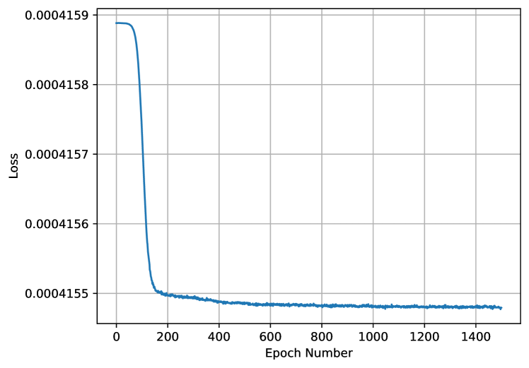
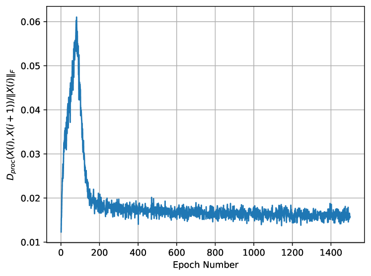
Refer to caption
(a) Loss function value as a function of number of epochs.
Refer to caption
(b) Change in embedding vectors versus epochs. The change is computed as the ratio of the Procrustes distance between embedding vectors in epoch i𝑖i and i+1𝑖1i+1 and the Frobenius norm of the embedding vectors in epoch i𝑖i.
Figure 10: Illustrating potential convergence issues associated with neural-network-based optimization of node embedding objectives.

Acknowledgments

This work was supported in part by the U.S. National Science Foundation under grant 1527618, the Department of Electrical and Computer Engineering, and the Division of Systems Engineering at Boston University. Any opinions, findings, and conclusions or recommendations expressed in this material are those of the author(s) and do not necessarily reflect the views of the supporting institutions.

References

  • [1] H. Cai, V. W. Zheng, and K. C.-C. Chang, “A comprehensive survey of graph embedding: Problems, techniques, and applications,” IEEE Transactions on Knowledge and Data Engineering, vol. 30, no. 9, pp. 1616–1637, 2018.
  • [2] B. Perozzi, R. Al-Rfou, and S. Skiena, “Deepwalk: Online learning of social representations,” in Proceedings of the 20th ACM SIGKDD international conference on Knowledge discovery and data mining.   ACM, 2014, pp. 701–710.
  • [3] Z. Yang, W. Cohen, and R. Salakhudinov, “Revisiting semi-supervised learning with graph embeddings,” in International conference on machine learning.   PMLR, 2016, pp. 40–48.
  • [4] A. Grover and J. Leskovec, “node2vec: Scalable feature learning for networks,” in Proceedings of the 22nd ACM SIGKDD international conference on Knowledge discovery and data mining.   ACM, 2016, pp. 855–864.
  • [5] W. Ding, C. Lin, and P. Ishwar, “Node embedding via word embedding for network community discovery,” IEEE Transactions on Signal and Information Processing over Networks, vol. 3, no. 3, pp. 539–552, 2017.
  • [6] T. Mikolov, I. Sutskever, K. Chen, G. S. Corrado, and J. Dean, “Distributed representations of words and phrases and their compositionality,” in Advances in neural information processing systems, 2013, pp. 3111–3119.
  • [7] J. Pennington, R. Socher, and C. Manning, “Glove: Global vectors for word representation,” in Proceedings of the 2014 conference on empirical methods in natural language processing (EMNLP), 2014, pp. 1532–1543.
  • [8] A. Bakarov, “A survey of word embeddings evaluation methods,” arXiv preprint arXiv:1801.09536, 2018.
  • [9] K. Rohe, S. Chatterjee, B. Yu et al., “Spectral clustering and the high-dimensional stochastic blockmodel,” Annals of Statistics, vol. 39, no. 4, pp. 1878–1915, 2011.
  • [10] D. L. Sussman, M. Tang, D. E. Fishkind, and C. E. Priebe, “A consistent adjacency spectral embedding for stochastic blockmodel graphs,” Journal of the American Statistical Association, vol. 107, no. 499, pp. 1119–1128, 2012.
  • [11] T. Qin and K. Rohe, “Regularized spectral clustering under the degree-corrected stochastic blockmodel,” in Advances in Neural Information Processing Systems, 2013, pp. 3120–3128.
  • [12] A. Athreya, D. E. Fishkind, M. Tang, C. E. Priebe, Y. Park, J. T. Vogelstein, K. Levin, V. Lyzinski, and Y. Qin, “Statistical inference on random dot product graphs: a survey,” Journal of machine learning research: JMLR, vol. 18, no. 1, pp. 8393–8484, Jan. 2017.
  • [13] K. Chaudhuri, F. Chung, and A. Tsiatas, “Spectral partitioning of graphs with general degrees and the extended planted partition model,” in Proceedings of the 25th conference on learning theory, vol. 2906, 2012.
  • [14] J. Cape, M. Tang, and C. E. Priebe, “On spectral embedding performance and elucidating network structure in stochastic blockmodel graphs,” Network Science, vol. 7, no. 3, pp. 269–291, 2019.
  • [15] J. Qiu, Y. Dong, H. Ma, J. Li, K. Wang, and J. Tang, “Network embedding as matrix factorization: Unifying deepwalk, line, pte, and node2vec,” in Proceedings of the Eleventh ACM International Conference on Web Search and Data Mining.   ACM, 2018, pp. 459–467.
  • [16] J. Tang, M. Qu, M. Wang, M. Zhang, J. Yan, and Q. Mei, “Line: Large-scale information network embedding,” in Proceedings of the 24th international conference on world wide web.   International World Wide Web Conferences Steering Committee, 2015, pp. 1067–1077.
  • [17] M. Girvan and M. Newman, “Girvan, m. & newman, m. e. j. community structure in social and biological networks. proc. natl acad. sci. usa 99, 7821-7826,” Proceedings of the National Academy of Sciences of the United States of America, vol. 99, pp. 7821–6, 07 2002.
  • [18] D. A. Spielman and S.-H. Teng, “Nearly-linear time algorithms for graph partitioning, graph sparsification, and solving linear systems,” in Proceedings of the thirty-sixth annual ACM symposium on Theory of computing.   ACM, 2004, pp. 81–90.
  • [19] R. Andersen, F. Chung, and K. Lang, “Local graph partitioning using pagerank vectors,” in Foundations of Computer Science, 2006. FOCS’06. 47th Annual IEEE Symposium on.   IEEE, 2006, pp. 475–486.
  • [20] R. Lambiotte, J.-C. Delvenne, and M. Barahona, “Random walks, markov processes and the multiscale modular organization of complex networks,” IEEE Transactions on Network Science and Engineering, vol. 1, no. 2, pp. 76–90, 2014.
  • [21] L. Meng and N. Masuda, “Analysis of node2vec random walks on networks,” Proceedings of the Royal Society A, vol. 476, no. 2243, p. 20200447, 2020.
  • [22] Y. Zhang and M. Tang, “Consistency of random-walk based network embedding algorithms,” arXiv preprint arXiv:2101.07354, 2021.
  • [23] L. Bottou, “Large-scale machine learning with stochastic gradient descent,” in Proceedings of COMPSTAT’2010.   Springer, 2010, pp. 177–186.
  • [24] ——, “Online algorithms and stochastic approximations,” in Online Learning and Neural Networks, D. Saad, Ed.   Cambridge, UK: Cambridge University Press, 1998, revised, oct 2012. [Online]. Available: http://leon.bottou.org/papers/bottou-98x
  • [25] B. Recht, C. Re, S. Wright, and F. Niu, “Hogwild: A lock-free approach to parallelizing stochastic gradient descent,” in Advances in Neural Information Processing Systems, 2011, pp. 693–701.
  • [26] H. White, S. Boorman, and R. Breiger, “Social structure from multiple networks, blockmodels of roles and positions,” American Journal of Sociology, pp. 730–780, 1976.
  • [27] P. Holland, K. Laskey, and S. Leinhardt, “Stochastic blockmodels: First steps,” Social Networks, vol. 5, no. 2, pp. 109–137, 1983.
  • [28] R. Boppana, “Eigenvalues and graph bisection: An average-case analysis,” in Proc. of the 28th Anuual Symposium on Foundations of Computer Science (FOCS), 1987, pp. 280–285.
  • [29] E. Abbe, A. S. Bandeira, and G. Hall, “Exact recovery in the stochastic block model,” IEEE transactions on information theory / Professional Technical Group on Information Theory, vol. 62, no. 1, pp. 471–487, Jan. 2016.
  • [30] E. Abbe and C. Sandon, “Community detection in general stochastic block models: Fundamental limits and efficient algorithms for recovery,” in Proc. of the 56th Annual Symposium on Foundations of Computer Science (FOCS), Sep. 2015, pp. 670–688.
  • [31] ——, “Detection in the stochastic block model with multiple clusters: proof of the achievability conjectures, acyclic bp, and the information-computation gap,” in Advances in Neural Information Processing Systems (NIPS), Dec. 2016.
  • [32] A. Decelle, F. Krzakala, C. Moore, and L. Zdeborová, “Asymptotic analysis of the stochastic block model for modular networks and its algorithmic applications,” Physical Review E, vol. 84, no. 6, p. 066106, 2011.
  • [33] E. Mossel, J. Neeman, and A. Sly, “Belief propagation, robust reconstruction and optimal recovery of block models,” in Proc. of the 27th Conference on Learning Theory (COLT), 2014, pp. 356–370.
  • [34] ——, “Reconstruction and estimation in the planted partition model,” Probability Theory and Related Fields, vol. 162, no. 3-4, pp. 431–461, Aug. 2015.
  • [35] O. Levy and Y. Goldberg, “Neural word embedding as implicit matrix factorization,” in Advances in neural information processing systems, 2014, pp. 2177–2185.
  • [36] K. Church and P. Hanks, “Word association norms, mutual information, and lexicography,” Computational linguistics, vol. 16, no. 1, pp. 22–29, 1990.
  • [37] M. E. Newman and M. Girvan, “Finding and evaluating community structure in networks,” Physical review E, vol. 69, no. 2, p. 026113, 2004.
  • [38] M. E. J. Newman, “Spectral methods for community detection and graph partitioning,” Physical review. E, Statistical, nonlinear, and soft matter physics, vol. 88, no. 4, p. 042822, Oct. 2013.
  • [39] M. Fazel, H. Hindi, and S. Boyd, “Rank minimization and applications in system theory,” in American Control Conference, 2004. Proceedings of the 2004, vol. 4.   IEEE, 2004, pp. 3273–3278.
  • [40] J. Dong, Z. Xue, J. Guan, Z.-F. Han, and W. Wang, “Low rank matrix completion using truncated nuclear norm and sparse regularizer,” Signal Processing: Image Communication, vol. 68, pp. 76–87, 2018.
  • [41] C. Lu, J. Feng, Y. Chen, W. Liu, Z. Lin, and S. Yan, “Tensor robust principal component analysis with a new tensor nuclear norm,” IEEE transactions on pattern analysis and machine intelligence, vol. 42, no. 4, pp. 925–938, 2019.
  • [42] B. Recht, M. Fazel, and P. A. Parrilo, “Guaranteed minimum-rank solutions of linear matrix equations via nuclear norm minimization,” SIAM review, vol. 52, no. 3, pp. 471–501, 2010.
  • [43] E. Hazan, “Sparse approximate solutions to semidefinite programs,” in Latin American symposium on theoretical informatics.   Springer, 2008, pp. 306–316.
  • [44] A. Joseph, B. Yu et al., “Impact of regularization on spectral clustering,” The Annals of Statistics, vol. 44, no. 4, pp. 1765–1791, 2016.
  • [45] U. Von Luxburg, “A tutorial on spectral clustering,” Statistics and computing, vol. 17, no. 4, pp. 395–416, 2007.
  • [46] R. Řehůřek and P. Sojka, “Software Framework for Topic Modelling with Large Corpora,” in Proceedings of the LREC 2010 Workshop on New Challenges for NLP Frameworks.   Valletta, Malta: ELRA, May 2010, pp. 45–50.
  • [47] F. Chollet et al., “Keras,” https://keras.io, 2015.
  • [48] S. M. Ross, J. J. Kelly, R. J. Sullivan, W. J. Perry, D. Mercer, R. M. Davis, T. D. Washburn, E. V. Sager, J. B. Boyce, and V. L. Bristow, Stochastic processes.   Wiley New York, 1996, vol. 2.
  • [49] C. McDiarmid, “On the method of bounded differences,” Surveys in combinatorics, vol. 141, no. 1, pp. 148–188, 1989.
  • [50] G. Grimmett and D. Stirzaker, Probability and random processes, 3rd Edition.   Oxford university press, 2001.