A simplified GW/BSE approach for charged and neutral excitation energies of large molecules and nanomaterials

Abstract

Inspired by Grimme’s simplified Tamm-Dancoff density functional theory approach [S. Grimme, J. Chem. Phys. 138, 244104 (2013)], we describe a simplified approach to excited state calculations within the GW approximation to the self-energy and the Bethe-Salpeter equation (BSE), which we call sGW/sBSE. The primary simplification to the electron repulsion integrals yields the same structure as with tensor hypercontraction, such that our method has a storage requirement that grows quadratically with system size and computational timing that grows cubically with system size. The performance of sGW is tested on the ionization potential of the molecules in the GW100 test set, for which it differs from ab intio GW calculations by only 0.2 eV. The performance of sBSE (based on sGW input) is tested on the excitation energies of molecules in the Thiel set, for which it differs from ab intio GW/BSE calculations by about 0.5 eV. As examples of the systems that can be routinely studied with sGW/sBSE, we calculate the band gap and excitation energy of hydrogen-passivated silicon nanocrystals with up to 2650 electrons in 4678 spatial orbitals and the absorption spectra of two large organic dye molecules with hundreds of atoms.

I Introduction

The GW approximation to the self-energy and the Bethe-Salpeter equation (BSE) are known to provide accurate charged and neutral excitation energies, respectively Hedin (1965); Strinati, Mattausch, and Hanke (1980); Hanke and Sham (1980); Strinati, Mattausch, and Hanke (1982); Strinati (1984); Hybertsen and Louie (1985, 1986); Albrecht et al. (1998); Rohlfing and Louie (2000). Given their successful application to solid-state materials, they have been increasingly applied to problems in molecular chemistry, for which they have been found to be affordable approaches with reasonable accuracy Tiago and Chelikowsky (2005); Faber et al. (2014); Körbel et al. (2014); Bruneval, Hamed, and Neaton (2015); Jacquemin, Duchemin, and Blase (2015); van Setten et al. (2015a); Caruso et al. (2016); Knight et al. (2016); Rangel et al. (2017). We refer to the reviews presented in Refs. Blase, Duchemin, and Jacquemin, 2018; Golze, Dvorak, and Rinke, 2019; Blase et al., 2020 for further information.

The computational cost of ab intio GW/BSE calculations depends on implementation details, which yield computational timings that scale as $N^{3}$ to $N^{6}$ with system size $N$ Foerster, Koval, and Sánchez-Portal (2011); Deslippe et al. (2012); van Setten, Weigend, and Evers (2013); Govoni and Galli (2015); Ljungberg et al. (2015); Krause and Klopper (2016); Bruneval et al. (2016); Wilhelm et al. (2018); Koval et al. (2019); Liu et al. (2020); Zhu and Chan (2021a); Bintrim and Berkelbach (2021) (throughout this work we exclusively consider the non-self-consistent G₀W₀ approximation but will typically refer to it as the GW approximation, for brevity). Although promising, the storage requirements and computational timing for ab intio GW/BSE calculations are still prohibitive for applications to very large systems or to problems requiring many calculations, such as averaging over the course of a molecular dynamics trajectory or in workflows for materials screening.

The same observations about computational costs of ab intio density functional theory (DFT) and time-dependent DFT (TDDFT) have led to a number of more affordable semiempirical approximations, including density functional tight-binding (DFTB) Elstner et al. (1998); Hourahine et al. (2020), extended tight-binding (xTB) Grimme, Bannwarth, and Shushkov (2017); Bannwarth, Ehlert, and Grimme (2019); Bannwarth et al. (2020). the simplified Tamm-Dancoff approximation (sTDA) to TDDFT, and combinations thereof, such as TD-DFTB Niehaus et al. (2001); Trani et al. (2011) and sTDA-xTB Grimme and Bannwarth (2016). Inspired in particular by Grimme’s sTDA, here we present a simplified GW/BSE approach that we call sGW/sBSE. As the heart of both approaches is a particular approximation to the electron repulsion integrals, which we show leads to a sGW/sBSE implementation with storage requirements that are quadratic in system size and execution times that are cubic in system size. Although sGW/sBSE results differ from ab intio ones by 0.1-1 eV, they can be applied to very large systems using only commodity computing resources.

II Theory

II.1 Integral approximations

A standard DFT calculation is first performed to yield the Kohn-Sham eigenvalues $\varepsilon_{p}$ and molecular orbitals (MOs) $\psi_{p}({\bm{r}})$. The MOs are expanded in a basis of atomic orbitals (AOs) $\phi_{\mu}({\bm{r}})$ or symetrically orthogonalized AOs $\phi^{\prime}_{\mu}({\bm{r}})$,

$$\psi_{p}({\bm{r}})=\sum_{\mu}\phi_{\mu}({\bm{r}})C_{\mu p}=\sum_{\mu}\phi^{\prime}_{\mu}({\bm{r}})C^{\prime}_{\mu p},$$ (1)

where $\mathbf{C}^{\prime}=\mathbf{S}^{1/2}\mathbf{C}$ and $\mathbf{S}$ is the AO overlap matrix. The primary simplification we make is to the four-center two-electron repulsion integrals (ERIs), whose storage and manipulation is responsible for much of the cost in correlated calculations with atom-centered basis functions. Following Grimme Grimme (2013), the MO ERIs are approximated to be (in 1122 notation)

$$(pq|rs)\approx\sum_{\mu\nu}L_{pq}^{\mu}L_{rs}^{\nu}J_{\mu\nu}=\sum_{\mu\nu}C^{\prime}_{\mu p}C^{\prime}_{\mu q}C^{\prime}_{\nu r}C^{\prime}_{\nu s}J_{\mu\nu}$$ (2)

where $L_{pq}^{\mu}=C^{\prime}_{\mu p}C^{\prime}_{\mu q}$ is the orthogonalized AO component of the orbital pair density. In the above, we are retaining (and approximating) only one- and two-center Coulomb integrals in the orthogonalized AO basis. The one-center Coulomb integrals are evaluated exactly, $J_{\mu\nu}^{(\mathrm{1c})}=(\mu\mu|\nu\nu)$, and the two-center Coulomb integrals are approximated by the Mataga-Nishimoto-Ohno-Klopman formula Nishimoto and Mataga (1957); Ohno (1964); Klopman (1964),

$$J_{\mu\nu}^{(\mathrm{2c})}\approx\left(\frac{1}{|r_{\mu}-r_{\nu}|^{2}+\eta_{\mu\nu}^{-2}}\right)^{-1/2},$$ (3)

where $\eta_{\mu\nu}=\left[(\mu\mu|\mu\mu)+(\nu\nu|\nu\nu)\right]/2$. The use of exact one-center integrals is a slight departure from the original sTDA method Grimme (2013).

The ERI approximation (2) has the same structure as the density fitting approximation (also known as the resolution of the identity approximation) Whitten (1973); Vahtras, Almlöf, and Feyereisen (1993); Feyereisen, Fitzgerald, and Komornicki (1993); Werner, Manby, and Knowles (2003), which have been regularly used in ab intio GW/BSE implementations with atom-centered basis sets Ren et al. (2012); Wilhelm, Ben, and Hutter (2016); Krause and Klopper (2016); Wilhelm et al. (2018); Koval et al. (2019); Liu et al. (2020); Zhu and Chan (2021a). However, we emphasize that the three-index tensors $L_{pq}^{\mu}$ are expressible as a product of two-index objects, the MO coefficients. Therefore, the standard density fitting procedure, requiring the calculation of two-center and three-center integrals and the solution of a system of linear equations, is completely bypassed (although we note that it may be used in the initial DFT calculation). More importantly, the final equality of Eq. (2) has the same structure as the ERIs with tensor hypercontraction Hohenstein, Parrish, and Martínez (2012), leading to an sGW/sBSE implementation that only requires the storage of two-index objects and opportunities for reductions in the scaling of the computational time.

II.2 Simplified GW

For the remainder of the manuscript, we will use $i,j,k,l$ to index occupied MOs in the Kohn-Sham reference, $a,b,c,d$ to index unoccupied MOs, and $p,q,r,s$ for general MOs. Within the diagonal G₀W₀ approximation, matrix elements of the self-energy operator are given by

$$\Sigma_{p}(\omega)=\Sigma_{p}^{\mathrm{(c)}}(\omega)-\sum_{i}(pi|ip).$$ (4)

The second term is the bare exchange part and the first term is the correlation part

$$\begin{split}\Sigma_{p}^{\mathrm{(c)}}(\omega)=\frac{i}{2\pi}\sum_{q}\int d\omega^{\prime}\frac{W_{pqqp}(\omega)-(pq|qp)}{\omega-\omega^{\prime}-\varepsilon_{q}+i\eta\textrm{sgn}(\varepsilon_{q}-\mu)},\end{split}$$ (5)

where $\eta$ is a positive infinitesimal and $\mu$ is the chemical potential. The screened Coulomb interaction is

$$W({\bm{r}}_{1},{\bm{r}}_{2};\omega)=\int d{\bm{r}}\varepsilon^{-1}({\bm{r}}_{1},{\bm{r}};\omega)|{\bm{r}}-{\bm{r}}_{2}|^{-1}$$ (6)

where the dielectric function is

$$\varepsilon({\bm{r}}_{1},{\bm{r}}_{2};\omega)=\delta({\bm{r}}_{1}-{\bm{r}}_{2})-\int d{\bm{r}}|{\bm{r}}_{1}-{\bm{r}}|^{-1}P({\bm{r}},{\bm{r}}_{2};\omega)$$ (7)

and the independent-particle polarizability is

$$\begin{split}P({\bm{r}}_{1},{\bm{r}}_{2};\omega)&=\sum_{ia}\psi_{a}({\bm{r}}_{1})\psi_{i}({\bm{r}}_{1})\psi_{i}({\bm{r}}_{2})\psi_{a}({\bm{r}}_{2})\\ &\hskip 10.00002pt\times\left[\frac{1}{\omega-(\varepsilon_{a}-\varepsilon_{i})+i\eta}-\frac{1}{\omega+(\varepsilon_{a}-\varepsilon_{i})+i\eta}\right].\end{split}$$ (8)

As mentioned above, Eq. (2) has the same structure as the density fitting approximation with $|\phi^{\prime}_{\mu}({\bm{r}})|^{2}$ playing the role of the auxiliary basis,

$$\psi_{p}({\bm{r}})\psi_{q}({\bm{r}})\approx\sum_{\mu}C_{\mu p}^{\prime}C_{\mu q}^{\prime}|\phi_{\mu}^{\prime}({\bm{r}})|^{2}=\sum_{\mu}L_{pq}^{\mu}|\phi_{\mu}^{\prime}({\bm{r}})|^{2}.$$ (9)

In this nonorthogonal auxiliary basis, the dielectric function has a matrix representation $\varepsilon_{\mu\nu}(\omega)\equiv[\bm{\varepsilon}(\omega)]_{\mu\nu}$ with

$$\bm{\varepsilon}(\omega) =\mathbf{S}^{\prime}-\mathbf{J}\mathbf{S}^{\prime-1}\mathbf{P}(\omega),$$ (10)

$$S_{\mu\nu}^{\prime} =\int d{\bm{r}}|\phi^{\prime}_{\mu}({\bm{r}})|^{2}|\phi^{\prime}_{\nu}({\bm{r}})|^{2},$$ (11)

$$P_{\mu\nu}(\omega) =\int d{\bm{r}}_{1}d{\bm{r}}_{2}|\phi^{\prime}_{\mu}({\bm{r}}_{1})|^{2}P({\bm{r}}_{1},{\bm{r}}_{2};\omega)|\phi^{\prime}_{\nu}({\bm{r}}_{2})|^{2}.$$ (12)

Rather than inverting the dielectric matrix at every frequency and numerically integrating, we use the plasmon-pole approximation Hybertsen and Louie (1986); von der Linden and Horsch (1988); Larson, Dvorak, and Wu (2013). Considering the generalized eigenvalue problem

$$\bm{\varepsilon}(\omega)\mathbf{U}(\omega)=\mathbf{S}^{\prime}\mathbf{U}(\omega)\bm{\lambda}(\omega),$$ (13)

we assume $\mathbf{U}(\omega)=\mathbf{U}(\omega=0)$ and that the eigenvalues can be parameterized by the form

$$\lambda_{l}^{-1}(\omega)=1+z_{l}\left(\frac{1}{\omega-(\omega_{l}-i\eta)}-\frac{1}{\omega+(\omega_{l}-i\eta)}\right).$$ (14)

The parameters $z_{l}$ and $\omega_{l}$ are chosen to match the numerical eigenvalues $\lambda_{l}(\omega)$ obtained at the two frequencies $\omega=0$ and $\omega=\varepsilon_{\mathrm{gap}}$ (i.e., the Kohn-Sham band gap). With this form, the frequency integration can be performed analytically to give

$$\begin{split}\Sigma^{\mathrm{(c)}}_{p}(\omega)&=\sum_{q\mu\nu}L_{pq}^{\mu}[\mathbf{S}^{\prime}\mathbf{U}\bm{\Lambda}^{(q)}(\omega)\mathbf{U}^{-1}\mathbf{S}^{\prime-1}\mathbf{J}]_{\mu\nu}L_{qp}^{\nu}\\ &=\sum_{ql}\left[\sum_{\mu}C_{\mu p}^{\prime}C_{\mu q}^{\prime}[\mathbf{S}^{\prime}\mathbf{U}]_{\mu l}\right]\Lambda^{(q)}_{ll}(\omega)\\ &\hskip 20.00003pt\times\left[\sum_{\nu}[\mathbf{U}^{-1}\mathbf{S}^{\prime-1}\mathbf{J}]_{l\nu}C_{\nu p}^{\prime}C_{\nu q}^{\prime}\right]\end{split}$$ (15)

where $\bm{\Lambda}^{(q)}(\omega)$ is a diagonal matrix with elements

$$\Lambda_{ll}^{(q)}(\omega)=\frac{z_{l}}{\omega-\varepsilon_{q}-\omega_{l}\textrm{sgn}(\varepsilon_{q}-\mu)}.$$ (16)

We calculate the GW quasiparticle energies $E_{p}$ using the linearized form

$$E_{p}=\varepsilon_{p}+Z_{p}\left[\Sigma_{p}(\varepsilon_{p})-v^{\mathrm{(xc)}}_{pp}\right]$$ (17)

where $v^{\mathrm{(xc)}}_{pp}$ is a diagonal matrix element of the DFT exchange-correlation potential and the renormalization factor is

$$Z_{p}=\left(1-\frac{\partial\Sigma(\omega)}{\partial\omega}\Big{|}_{\varepsilon_{p}}\right)^{-1}.$$ (18)

Using only $O(N^{2})$ storage, the intermediates indicated in square brackets in Eq. (15) can be formed for each orbital $p$ of interest in $O(N^{3})$ time; the time needed to calculate $n_{\mathrm{GW}}$ eigenvalues is then $O(n_{\mathrm{GW}}N^{3})$. If $O(N^{3})$ storage is available, then the intermediates indicated can be calculated once and stored as a three-index object; the time needed to calculate all eigenvalues is then only $O(N^{3})$.

Finally, we note that the full self-energy (4) requires bare MO exchange integrals. Within sGW/sBSE, three options exist. When the initial DFT calculation is done with a pure local functional, then the MO exchange integrals can be approximated by Eq. (2). This allows the exchange contribution for all matrix elements of the self-energy to be calculated in $O(N^{3})$ time. In numerical tests (not shown), this was found to be a poor approximation, which we believe to be a worthy topic of future study. Therefore, as a second option, we consider modifying the ERI approximation to include one-center AO exchange integrals,

$$(pq|rs)\approx\sum_{\mu\nu}L_{pq}^{\mu}L_{rs}^{\nu}J_{\mu\nu}+\sum_{\mu\neq\nu}^{(\mathrm{1c})}\left(L_{pr}^{\mu}L_{qs}^{\nu}+L_{ps}^{\mu}L_{qr}^{\nu}\right)K_{\mu\nu}^{(\mathrm{1c})}.$$ (19)

The one-center AO exchange integrals are empirically scaled by a single parameter, $K_{\mu\nu}=\alpha_{K}(\mu\nu|\mu\nu)$, and the AO ERIs $(\mu\nu|\mu\nu)$ are calculated exactly. This improvement adds negligible computational cost with only $O(N^{2})$ scaling. To motivate the third and final option, we recall that hybrid functionals often provide a better starting point for G₀W₀/BSE calculations Caruso et al. (2016); Jacquemin et al. (2017); Blase et al. (2020). In this case, matrix elements of the exchange operator are already available and can be reused for free in the evaluation of the GW self-energy. We will present results for both the second and third options in Sec. III.1.

II.3 Simplified BSE

Within the Tamm-Dancoff and static screening approximations, the BSE is an eigenvalue problem for the matrix

$$A_{ia,jb}=(E_{a}-E_{i})\delta_{ij}\delta_{ab}+\alpha(ia|jb)-(ij|W|ab),$$ (20)

where $\alpha=2$ for singlets and 0 for triplets. Note that GW quasiparticle energies $E_{p}$ are required as input to a BSE calculation; sGW energies will be used in sBSE calculations. With the integral simplification (2) and the static screening approximation to the screened Coulomb interaction (6), in sBSE we have

$$(ij|W|ab) =\sum_{\mu\nu}L_{ij}^{\mu}L_{ab}^{\nu}W_{\mu\nu}=\sum_{\mu\nu}C^{\prime}_{\mu i}C^{\prime}_{\mu j}C^{\prime}_{\nu a}C^{\prime}_{\nu b}W_{\mu\nu}$$ (21a)

$$\mathbf{W} =\mathbf{S}^{\prime}\bm{\varepsilon}^{-1}(\omega=0)\mathbf{J}$$ (21b)

Note that $(ij|W|ab)$ has the same structure as the bare $(ij|ab)$, with $W_{\mu\nu}$ replacing $J_{\mu\nu}$, and that $W_{\mu\nu}$ can be built simply by matrix multiplication, requiring only quadratic storage and cubic CPU time. We discuss further computational costs of sBSE below.

For comparison, we also provide results obtained by the simplified TDA (sTDA) approach Grimme (2013), which is a structurally identical eigenvalue problem for the matrix

$$A_{ia,jb}=(\varepsilon_{a}-\varepsilon_{i})\delta_{ij}\delta_{ab}+\alpha(ia|jb)-a_{x}(ij|ab),$$ (22)

where $a_{x}$ is the fraction of exact exchange included in the DFT functional. Our sTDA calculations closely follow Ref. Grimme, 2013 except that we use exact one-center integrals, as mentioned in Sec. II.1. Clearly the only two differences between sBSE and sTDA are the use of sGW or DFT eigenvalues and the use of a screened Coulomb interaction or a rescaled bare Coulomb interaction. For solids or heterogeneous nanostructures, it is expected that the screening in sBSE provides a more accurate treatment of the electron-hole interaction.

Select eigenvalues of the sTDA or sBSE matrices can be found by iterative eigensolvers, like the Davidson algorithm, that require only matrix-vector products and the $O(N^{2})$ storage of trial vectors $c_{i}^{a}$. With the integral approximations (2) and (21), the sTDA and sBSE matrix-vector product can be done with $O(N^{2})$ storage in $O(N^{3})$ time,

$$\begin{split}[\mathbf{Ac}]_{ia}&=(E_{a}-E_{i})c_{i}^{a}+\alpha\sum_{\mu}C^{\prime}_{\mu i}C^{\prime}_{\mu a}\sum_{\nu}J_{\mu\nu}\sum_{jb}C^{\prime}_{\nu j}C^{\prime}_{\nu b}c_{j}^{b}\\ &\hskip 10.00002pt-\sum_{\mu}C^{\prime}_{\mu i}\sum_{\nu}C^{\prime}_{\nu a}W_{\mu\nu}\sum_{j}C^{\prime}_{\mu j}\sum_{b}C^{\prime}_{\nu b}c_{j}^{b}\end{split}$$ (23)

with intermediate formation as indicated. In fact, if only a few sBSE eigenvalues are desired and only $O(N^{2})$ storage is available, then the calculation of the sGW eigenvalues to be used in the sBSE is more expensive than finding the few eigenvalues of the sBSE matrix.

III Results

All calculations (DFT, GW/BSE, and sGW/sBSE) were performed using a locally modified version of the PySCF software package Sun et al. (2018, 2020); Zhu and Chan (2021a) using the TZVP basis set Schäfer, Huber, and Ahlrichs (1994). DFT calculations used the B3LYP exchange-correlation functional unless stated otherwise.

III.1 Simplified GW

The performance of sGW is assessed with the first ionization potential (highest occupied molecular orbital energy) of the atoms and molecules in the GW100 test set van Setten et al. (2015a); the TZVP basis set is used for all atoms except I, Xe, and Rb for which the DZVP basis set Godbout et al. (1992) is used. We assess the accuracy of sGW by comparing to ab intio, full-frequency GW calculations (i.e., without the plasmon pole approximation) using the same basis set.

We first address the evaluation of the bare exchange part of the self-energy. As mentioned previously, it can be approximated by Eq. (2), Eq. (19), or calculated exactly, which is free when a hybrid functional is used in the DFT reference. Figure 1(a) compares the IPs from ab intio GW to those of sGW when approximate [Eq. (19)] or exact exchange integrals are used. With approximate exchange integrals, the single free parameter $\alpha_{K}$ is optimized to minimize the mean absolute error (MAE) with respect to the ab intio GW calculations, which leads to $\alpha_{K}=0.46$; this value was found to be robust to the basis set or exchange-correlation functional used. This approximate treatment of exchange integrals gives a reasonable estimate of the IP with a MAE of 1.81 eV (note that the IPs of the test set range from $-25$ to $-3$ eV). The use of the exact exchange integrals greatly increases the accuracy, giving a MAE of only 0.20 eV. Figure 1(b) shows that sGW also gives good agreement with experimental IPs van Setten et al. (2015a), especially when exact exchange is used. Therefore, for the rest of this study, the exact exchange integrals are used, but we will return to this point in Sec. IV.

Figure 1: First ionization potential of the molecules in the GW100 set calculated by sGW@B3LYP compared to (a) ab initio GW@B3LYP results and (b) experiment, using an approximate (light) and exact (dark) bare exchange matrix element.

Table 1 summarizes the MAE and mean signed error (MSE) of the ab initio GW and sGW IPs compared to experimental values. The GW and sGW calculations used PBE, PBE0, and B3LYP references; for PBE, we calculated the exact diagonal matrix element of the exchange operator after the SCF convergence. Calculations using the hybrid functionals PBE0 and B3LYP are about 0.2 eV more accurate than those with the PBE functional. The difference in the performance of the ab initio GW and sGW is marginal, indicating an accurate estimation of the correlation term of the self-energy by sGW. As will be demonstrated in Sec. III.3, the cost of the sGW calculations is significantly smaller than that of the ab intio GW calculations.

Table 1: Mean absolute error (MAE) and mean signed error (MSE) of the first ionization potential of the molecules in the GW100 test set with respect to ab initio GW and experimental values. Errors are in eV and exact exchange matrix elements were used in the sGW calculations.

	PBE		PBE0		B3LYP
	GW	sGW	GW	sGW	GW	sGW
MAE wrt GW	-	0.23	-	0.19	-	0.20
MSE wrt GW	-	$-0.01$	-	$-0.03$	-	$-0.04$
MAE wrt Expt	0.89	0.93	0.68	0.69	0.72	0.72
MSE wrt Expt	0.85	0.84	0.57	0.53	0.62	0.58

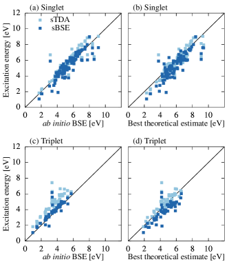
Figure 2: Singlet excitation energies of the 28 molecules in Thiel’s set calculated by sBSE compared to (a) ab initio sBSE results and (b) best theoretical estimtes. Analogous results for triplet excitation energies are shown in (c) and (d).

Table 2: Mean absolute error (MAE) and mean signed error (MSE) of singlet and triplet excitation energies of Thiel’s set with respect to ab initio BSE and best theoretical estimates (BTE). Errors are in eV.

	Singlet			Triplet
	BSE	sBSE	sTDA	BSE	sBSE	sTDA
MAE wrt BSE	-	0.51	0.47	-	0.38	1.22
MSE wrt BSE	-	$-0.10$	0.31	-	0.27	1.22
MAE wrt BTE	0.50	0.71	0.44	0.93	0.81	0.47
MSE wrt BTE	$-0.46$	$-0.56$	$-0.15$	$-0.93$	-0.66	0.29

III.2 Simplified BSE

Neutral excitation energies calculated by sTDA and sGW/sBSE are tested on a set of 28 organic molecules commonly known as Thiel’s set Schreiber et al. (2008); Silva-Junior et al. (2008). Figure 2 compares 97 singlet states and 51 triplet states calculated by sBSE to those calculated by ab initio BSE and to the best theoretical estimates from higher level methods proposed by Thiel and coworkers Schreiber et al. (2008); Silva-Junior et al. (2008). The ab initio BSE calculations are done using full-frequency GW eigenvalues, with ab initio static screening of the Coulomb interaction (i.e., without the plasmon-pole approximation), and without the Tamm-Dancoff approximation. The MAEs and MSEs are summarized in Tab. 2. The MAEs of singlet and triplet excitations calculated by sBSE with respect to ab initio BSE are 0.51 eV and 0.38 eV, respectively, which are similar to the errors exhibited by sGW. The MAEs of singlet and triplet excitations calculated by sBSE with respect to the theoretical best estimates are 0.71 eV and 0.81 eV, respectively, which are similar to the errors exhibited by ab initio BSE. Once again we conclude that the performance difference between ab initio BSE and sBSE is marginal. Interestingly, we note that sTDA gives similar but slightly smaller errors when compared to the best theoretical estimates.

III.3 Applications

Having demonstrated the accuracy of the sGW/sBSE framework on benchmark sets of small molecules, we move on to study silicon clusters as a prototypical semiconductor nanomaterial. Specifically, we study hydrogen-passivated silicon clusters ranging from SiH₄ to Si₁₈₁H₁₁₆, which has 2650 electrons and 4678 spatial orbitals. Calculations on larger clusters were limited by the cost of the initial DFT calculation. The structure of SiH₄ is from the GW100 set van Setten et al. (2015b), the structures of Si₅H₁₂ and Si₁₀H₁₆ are from PubChem pub (2021), and the structures of larger clusters are from CSIRO Nanostructure Data Bank Wilson, McKenzie-Sell, and Barnard (2014), without further geometry relaxation. In Fig. 3(a), we show the quasiparticle gap (calculated by DFT and sGW) and the first neutral excitation energy (calculated by sBSE) as a function of the cluster diameter, which is estimated by approximating the cluster as a sphere with a number density equal to that of bulk silicon (50 atoms/nm³). For comparison, we show experimental photoluminescence energies from Ref. Wolkin et al., 1999. The large system sizes accessible with sGW/sBSE allow us to compare directly to these experimental values. We see that the sBSE excitation energies are about 1 eV higher than experiment, which may be due to a vibrational Stokes shift, finite-temperature effects, differences in structure, or inaccuracies in the GW/BSE level of theory.

Figure 3(b) shows the CPU time of each method as a function of number of electrons in the silicon clusters. In practice, most calculations are performed with some degree of parallelism using up to 32 cores; thus, while we report the total CPU time, the wall time can be significantly less. For sGW, we report the CPU time required per eigenvalue using the algorithm that requires only $O(N^{2})$ storage, such that we expect $O(N^{3})$ scaling, which is confirmed numerically. The savings afforded by our sGW algorithm enabled us to calculate about 2500 GW orbital energies on our largest system (with 2650 electrons and 4678 total orbitals) in about three days using a single 32-core node. The sBSE calculations were performed in a truncated space that included those orbitals with energies between 30 eV below the highest occupied orbital and 30 eV above the lowest unoccupied orbital. Again we report the CPU time required per eigenvalue, such that we expect $O(N^{3})$ scaling, which is confirmed numerically. In practice, we were able to calculate 50 excitation energies on the largest nanocluster in less than an hour. We note that the sBSE calculations are less expensive than the preceding sGW calculations.

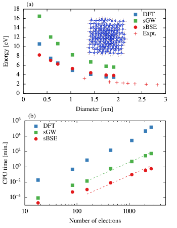
Figure 3: (a) Quasiparticle gap calculated by DFT (B3LYP) and sGW@B3LYP and first excitation energy calculated by sBSE of silicon nanoclusters. Experimental results (plus signs) were determined in Ref. Wolkin et al., 1999 by photoluminescence. Also shown is the molecular structure of the largest studied cluster, Si₁₈₁H₁₁₆, which has 2650 electrons and 4678 orbitals in the TZVP basis set. (b) CPU time required for DFT and CPU time required per eigenvalue for sGW and sBSE calculations. The sBSE calculations used a truncated set of orbitals. The dashed lines show $N^{3}$ power laws.

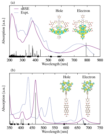
Figure 4: Absorption spectra of (a) an organic dye molecule and (b) a chlorophyll-based donor-bridge-acceptor molecule. Black vertical lines indicate the relative oscillator strength of each transition calculated by sBSE. Squares show the transitions with vanishing oscillator strength. Natural transition orbitals of the transitions at 792 nm (a) and 677 nm (b) are shown as insets.

As a final class of example problems, we apply sGW/sBSE to study the optical properties of large organic molecules. In Fig. 4, we show the absorption spectra of a 192-atom organic dye molecule and a 126-atom chlorophyll-based donor-bridge-acceptor dyad, whose structures and experimetal spectra are taken from Refs. Grimme and Bannwarth, 2016 and Huang et al., 2016, respectively. Considering that solvent effects and vibrational dynamics are neglected, the agreement between sBSE and experiment is quite good. As shown in Fig. 4(a), the organic dye molecule has a broad peak between 700 and 800 nm and strong peak at 360 nm; the sBSE predicts a slightly redshifted broad peak, but correctly predicts the strong peak at 360 nm, including its lineshape. As shown in Fig. 4(b), the chlorophyll molecule has two prototypical strong peaks, the so-called Q band and Soret band. The sBSE reproduces the Q band near 650 nm and the strong Soret band around 430 nm. However, we note that some transitions are spectroscopically dark at the equilibrium geometry but the experimental spectrum shows clear vibronic signatures, indicating the likely importance of nuclear dynamics for total agreement. Despite being a semiempirical method, sBSE yields a proper excited-state wavefunction, enabling a variety of analyses. As an example, in Fig. 4, we show the largest-weight natural transition orbitals (NTOs) Martin (2003) of one low-lying transition of each molecule (NTOs are the electron-hole orbital pair that best represent the transition). Clearly, the NTOs show that the two analyzed excitations are relatively localized to specific regions of the molecules.

IV Conclusions and future work

We have presented the simplified GW and BSE methods, which we call sGW/sBSE. In addition to the plasmon-pole and static screening approximations, an approximation to the electron repulsion integrals first used in Ref. Grimme, 2013 is most responsible for the low cost of sGW/sBSE. The sGW/sBSE results are in good agreement with ab initio results as well as those of experiments or higher-level methods. In its present form, we expect that sGW/sBSE can facilitate rapid, semiquantitative calculations of charged and neutral excitations of large molecules and nanomaterials.

An obvious limitation of the present sGW/sBSE framework is its reliance on an initial ab initio DFT calculation, especially when hybrid functionals are used, as can be seen from Fig. 3(b). Future work will address the replacement of DFT with a semiempirical mean-field theory, similar to the combination of the extended tight-binding method (xTB) with the sTDA for extremely affordable calculations of excitation energies Grimme and Bannwarth (2016). Additionally, we plan to implement spin-orbit coupling and Brillouin zone sampling for periodic systems. More generally, sGW/sBSE could be made into a more ab initio method by pursuing similar structure through tensor decompositions or integral screening. Lastly, we believe that the sGW/sBSE framework could be used as an affordable testing ground for improvements to the GW/BSE formalism, such as self-consistency, vertex corrections Shishkin, Marsman, and Kresse (2007); Romaniello, Guyot, and Reining (2009); Maggio and Kresse (2017); Lewis and Berkelbach (2019), or the combination of GW with dynamical mean-field theory Biermann, Aryasetiawan, and Georges (2003); Zhu and Chan (2021b).

References

- Hedin (1965) L. Hedin, Phys. Rev. 139, A796 (1965).
- Strinati, Mattausch, and Hanke (1980) G. Strinati, H. J. Mattausch, and W. Hanke, Phys. Rev. Lett. 45, 290 (1980).
- Hanke and Sham (1980) W. Hanke and L. J. Sham, Phys. Rev. B 21, 4656 (1980).
- Strinati, Mattausch, and Hanke (1982) G. Strinati, H. J. Mattausch, and W. Hanke, Phys. Rev. B 25, 2867 (1982).
- Strinati (1984) G. Strinati, Phys. Rev. B 29, 5718 (1984).
- Hybertsen and Louie (1985) M. S. Hybertsen and S. G. Louie, Phys. Rev. Lett. 55, 1418 (1985).
- Hybertsen and Louie (1986) M. S. Hybertsen and S. G. Louie, Phys. Rev. B 34, 5390 (1986).
- Albrecht et al. (1998) S. Albrecht, L. Reining, R. D. Sole, and G. Onida, Phys. Status Solidi 170, 189 (1998).
- Rohlfing and Louie (2000) M. Rohlfing and S. G. Louie, Phys. Rev. B 62, 4927 (2000).
- Tiago and Chelikowsky (2005) M. L. Tiago and J. R. Chelikowsky, Solid State Commun. 136, 333 (2005).
- Faber et al. (2014) C. Faber, P. Boulanger, C. Attaccalite, I. Duchemin, and X. Blase, Philos. Trans. Royal Soc. A 372, 20130271 (2014).
- Körbel et al. (2014) S. Körbel, P. Boulanger, I. Duchemin, X. Blase, M. A. L. Marques, and S. Botti, J. Chem. Theory Comput. 10, 3934 (2014).
- Bruneval, Hamed, and Neaton (2015) F. Bruneval, S. M. Hamed, and J. B. Neaton, J. Chem. Phys. 142, 244101 (2015).
- Jacquemin, Duchemin, and Blase (2015) D. Jacquemin, I. Duchemin, and X. Blase, J. Chem. Theory Comput. 11, 3290 (2015).
- van Setten et al. (2015a) M. J. van Setten, F. Caruso, S. Sharifzadeh, X. Ren, M. Scheffler, F. Liu, J. Lischner, L. Lin, J. R. Deslippe, S. G. Louie, C. Yang, F. Weigend, J. B. Neaton, F. Evers, and P. Rinke, J. Chem. Theory Comput. 11, 5665 (2015a).
- Caruso et al. (2016) F. Caruso, M. Dauth, M. J. van Setten, and P. Rinke, J. Chem. Theory Comput. 12, 5076 (2016).
- Knight et al. (2016) J. W. Knight, X. Wang, L. Gallandi, O. Dolgounitcheva, X. Ren, J. V. Ortiz, P. Rinke, T. Körzdörfer, and N. Marom, J. Chem. Theory Comput. 12, 615 (2016).
- Rangel et al. (2017) T. Rangel, S. M. Hamed, F. Bruneval, and J. B. Neaton, J. Chem. Phys. 146, 194108 (2017).
- Blase, Duchemin, and Jacquemin (2018) X. Blase, I. Duchemin, and D. Jacquemin, Chem. Soc. Rev. 47, 1022 (2018).
- Golze, Dvorak, and Rinke (2019) D. Golze, M. Dvorak, and P. Rinke, Front. Chem. 7, 377 (2019).
- Blase et al. (2020) X. Blase, I. Duchemin, D. Jacquemin, and P.-F. Loos, J. Phys. Chem. Lett. 11, 7371 (2020).
- Foerster, Koval, and Sánchez-Portal (2011) D. Foerster, P. Koval, and D. Sánchez-Portal, J. Chem. Phys. 135, 074105 (2011).
- Deslippe et al. (2012) J. Deslippe, G. Samsonidze, D. A. Strubbe, M. Jain, M. L. Cohen, and S. G. Louie, Comput. Phys. Commun. 183, 1269 (2012).
- van Setten, Weigend, and Evers (2013) M. J. van Setten, F. Weigend, and F. Evers, J. Chem. Theory Comput. 9, 232 (2013).
- Govoni and Galli (2015) M. Govoni and G. Galli, J. Chem. Theory Comput. 11, 2680 (2015).
- Ljungberg et al. (2015) M. P. Ljungberg, P. Koval, F. Ferrari, D. Foerster, and D. Sánchez-Portal, Phys. Rev. B 92, 075422 (2015).
- Krause and Klopper (2016) K. Krause and W. Klopper, J. Comput. Chem. 38, 383 (2016).
- Bruneval et al. (2016) F. Bruneval, T. Rangel, S. M. Hamed, M. Shao, C. Yang, and J. B. Neaton, Comput. Phys. Commun. 208, 149 (2016).
- Wilhelm et al. (2018) J. Wilhelm, D. Golze, L. Talirz, J. Hutter, and C. A. Pignedoli, J. Phys. Chem. Lett. 9, 306 (2018).
- Koval et al. (2019) P. Koval, M. P. Ljungberg, M. Müller, and D. Sánchez-Portal, J. Chem. Theory Comput. 15, 4564 (2019).
- Liu et al. (2020) C. Liu, J. Kloppenburg, Y. Yao, X. Ren, H. Appel, Y. Kanai, and V. Blum, J. Chem. Phys. 152, 044105 (2020).
- Zhu and Chan (2021a) T. Zhu and G. K.-L. Chan, J. Chem. Theory Comput. 17, 727 (2021a).
- Bintrim and Berkelbach (2021) S. J. Bintrim and T. C. Berkelbach, J. Chem. Phys. 154, 041101 (2021).
- Elstner et al. (1998) M. Elstner, D. Porezag, G. Jungnickel, J. Elsner, M. Haugk, T. Frauenheim, S. Suhai, and G. Seifert, Phys. Rev. B 58, 7260 (1998).
- Hourahine et al. (2020) B. Hourahine, B. Aradi, V. Blum, F. Bonafé, A. Buccheri, C. Camacho, C. Cevallos, M. Deshaye, T. Dumitrică, A. Dominguez, et al., J. Chem. Phys. 152, 124101 (2020).
- Grimme, Bannwarth, and Shushkov (2017) S. Grimme, C. Bannwarth, and P. Shushkov, J. Chem. Theory Comput. 13, 1989 (2017).
- Bannwarth, Ehlert, and Grimme (2019) C. Bannwarth, S. Ehlert, and S. Grimme, J. Chem. Theory Comput. 15, 1652 (2019).
- Bannwarth et al. (2020) C. Bannwarth, E. Caldeweyher, S. Ehlert, A. Hansen, P. Pracht, J. Seibert, S. Spicher, and S. Grimme, WIREs Comput. Mol. Sci. 11 (2020), 10.1002/wcms.1493.
- Niehaus et al. (2001) T. A. Niehaus, S. Suhai, F. Della Sala, P. Lugli, M. Elstner, G. Seifert, and T. Frauenheim, Phys. Rev. B 63, 085108 (2001).
- Trani et al. (2011) F. Trani, G. Scalmani, G. Zheng, I. Carnimeo, M. J. Frisch, and V. Barone, J. Chem. Theory Comput. 7, 3304 (2011).
- Grimme and Bannwarth (2016) S. Grimme and C. Bannwarth, J. Chem. Phys. 145, 054103 (2016).
- Grimme (2013) S. Grimme, J. Chem. Phys. 138, 244104 (2013).
- Nishimoto and Mataga (1957) K. Nishimoto and N. Mataga, Z. Phys. Chem. 12, 335 (1957).
- Ohno (1964) K. Ohno, Theor. Chim. Acta 2, 219 (1964).
- Klopman (1964) G. Klopman, J. Am. Chem. Soc. 86, 4550 (1964).
- Whitten (1973) J. L. Whitten, J. Chem. Phys. 58, 4496 (1973).
- Vahtras, Almlöf, and Feyereisen (1993) O. Vahtras, J. Almlöf, and M. Feyereisen, Chem. Phys. Lett. 213, 514 (1993).
- Feyereisen, Fitzgerald, and Komornicki (1993) M. Feyereisen, G. Fitzgerald, and A. Komornicki, Chem. Phys. Lett. 208, 359 (1993).
- Werner, Manby, and Knowles (2003) H.-J. Werner, F. R. Manby, and P. J. Knowles, J. Chem. Phys. 118, 8149 (2003).
- Ren et al. (2012) X. Ren, P. Rinke, V. Blum, J. Wieferink, A. Tkatchenko, A. Sanfilippo, K. Reuter, and M. Scheffler, New J. Phys. 14, 053020 (2012).
- Wilhelm, Ben, and Hutter (2016) J. Wilhelm, M. D. Ben, and J. Hutter, J. Chem. Theory Comput. 12, 3623 (2016).
- Hohenstein, Parrish, and Martínez (2012) E. G. Hohenstein, R. M. Parrish, and T. J. Martínez, J. Chem. Phys. 137, 044103 (2012).
- von der Linden and Horsch (1988) W. von der Linden and P. Horsch, Phys. Rev. B 37, 8351 (1988).
- Larson, Dvorak, and Wu (2013) P. Larson, M. Dvorak, and Z. Wu, Phys. Rev. B 88, 125205 (2013).
- Jacquemin et al. (2017) D. Jacquemin, I. Duchemin, A. Blondel, and X. Blase, J. Chem. Theory Comput. 13, 767 (2017).
- Sun et al. (2018) Q. Sun, T. C. Berkelbach, N. S. Blunt, G. H. Booth, S. Guo, Z. Li, J. Liu, J. D. McClain, E. R. Sayfutyarova, S. Sharma, et al., WIREs Comput. Mol. Sci. 8, e1340 (2018).
- Sun et al. (2020) Q. Sun, X. Zhang, S. Banerjee, P. Bao, M. Barbry, N. S. Blunt, N. A. Bogdanov, G. H. Booth, J. Chen, Z.-H. Cui, J. J. Eriksen, Y. Gao, S. Guo, J. Hermann, M. R. Hermes, K. Koh, P. Koval, S. Lehtola, Z. Li, J. Liu, N. Mardirossian, J. D. McClain, M. Motta, B. Mussard, H. Q. Pham, A. Pulkin, W. Purwanto, P. J. Robinson, E. Ronca, E. R. Sayfutyarova, M. Scheurer, H. F. Schurkus, J. E. T. Smith, C. Sun, S.-N. Sun, S. Upadhyay, L. K. Wagner, X. Wang, A. White, J. D. Whitfield, M. J. Williamson, S. Wouters, J. Yang, J. M. Yu, T. Zhu, T. C. Berkelbach, S. Sharma, A. Y. Sokolov, and G. K.-L. Chan, J. Chem. Phys. 153, 024109 (2020).
- Schäfer, Huber, and Ahlrichs (1994) A. Schäfer, C. Huber, and R. Ahlrichs, J. Chem. Phys. 100, 5829 (1994).
- Godbout et al. (1992) N. Godbout, D. R. Salahub, J. Andzelm, and E. Wimmer, Can. J. Chem. 70, 560 (1992).
- Schreiber et al. (2008) M. Schreiber, M. R. Silva-Junior, S. P. Sauer, and W. Thiel, J. Chem. Phys. 128, 134110 (2008).
- Silva-Junior et al. (2008) M. R. Silva-Junior, M. Schreiber, S. P. Sauer, and W. Thiel, J. Chem. Phys. 129, 104103 (2008).
- van Setten et al. (2015b) M. J. van Setten, F. Caruso, S. Sharifzadeh, X. Ren, M. Scheffler, F. Liu, J. Lischner, L. Lin, J. R. Deslippe, S. G. Louie, et al., J. Chem. Theory Comput. 11, 5665 (2015b).
- pub (2021) “National center for biotechnology information,” (2021), pubChem Compound Summary for CID 71353974 and 101946798. https://pubchem.ncbi.nlm.nih.gov. Accessed July 1, 2021.
- Wilson, McKenzie-Sell, and Barnard (2014) H. F. Wilson, L. McKenzie-Sell, and A. S. Barnard, J. Mater. Chem. C 2, 9451 (2014).
- Wolkin et al. (1999) M. Wolkin, J. Jorne, P. Fauchet, G. Allan, and C. Delerue, Phys. Rev. Lett. 82, 197 (1999).
- Huang et al. (2016) G.-J. Huang, M. A. Harris, M. D. Krzyaniak, E. A. Margulies, S. M. Dyar, R. J. Lindquist, Y. Wu, V. V. Roznyatovskiy, Y.-L. Wu, R. M. Young, et al., J. Phys. Chem. B 120, 756 (2016).
- Martin (2003) R. L. Martin, J. Chem. Phys. 118, 4775 (2003).
- Shishkin, Marsman, and Kresse (2007) M. Shishkin, M. Marsman, and G. Kresse, Phys. Rev. Lett. 99, 246403 (2007).
- Romaniello, Guyot, and Reining (2009) P. Romaniello, S. Guyot, and L. Reining, J. Chem. Phys. 131, 154111 (2009).
- Maggio and Kresse (2017) E. Maggio and G. Kresse, J. Chem. Theory Comput. 13, 4765 (2017).
- Lewis and Berkelbach (2019) A. M. Lewis and T. C. Berkelbach, J. Chem. Theory Comput. 15, 2925 (2019).
- Biermann, Aryasetiawan, and Georges (2003) S. Biermann, F. Aryasetiawan, and A. Georges, Phys. Rev. Lett. 90, 086402 (2003).
- Zhu and Chan (2021b) T. Zhu and G. K.-L. Chan, Phys. Rev. X 11, 021006 (2021b).