All Bark and No Bite: Rogue Dimensions in Transformer Language Models Obscure Representational Quality

Abstract

Similarity measures are a vital tool for understanding how language models represent and process language. Standard representational similarity measures such as cosine similarity and Euclidean distance have been successfully used in static word embedding models to understand how words cluster in semantic space. Recently, these measures have been applied to embeddings from contextualized models such as BERT and GPT-2. In this work, we call into question the informativity of such measures for contextualized language models. We find that a small number of rogue dimensions, often just 1-3, dominate these measures. Moreover, we find a striking mismatch between the dimensions that dominate similarity measures and those which are important to the behavior of the model. We show that simple postprocessing techniques such as standardization are able to correct for rogue dimensions and reveal underlying representational quality. We argue that accounting for rogue dimensions is essential for any similarity-based analysis of contextual language models.

1 Introduction

By mapping words into continuous vector spaces, we can reason about human language in geometric terms. For example, the cosine similarity of pairs of word embeddings in Word2Vec Mikolov et al. (2013) and GloVe Pennington et al. (2014) shows a robust correlation with human similarity judgments, and embeddings cluster into natural semantic classes in Euclidean space Baroni et al. (2014); Wang et al. (2019). In recent years, static embeddings have given way to their contextual counterparts, with language models based on the transformer architecture Vaswani et al. (2017) such as BERT Devlin et al. (2019), RoBERTa Liu et al. (2020), XLNet Yang et al. (2019) and GPT-2 Radford et al. (2019) achieving state of the art results on many language understanding tasks. Despite their success, relatively little is known about how these models represent and process language. Recent work has employed measures such as cosine similarity and Euclidean distance to contextual representations with unclear and counterintuitive results. For example, similarity/distance measures in BERT are extremely sensitive to word position, leading to inconsistent results on evaluation benchmarks Mickus et al. (2020); May et al. (2019). Additionally, representational quality appears to degrade severely in later layers of each network, with the final layers of BERT, RoBERTa, GPT-2 and XLNet showing little to no correlation with the semantic similarity/relatedness judgments of humans Bommasani et al. (2020).

Recent work which probes the representational geometry of contextualized embedding spaces using cosine similarity has found that contextual embeddings have several counterintuitive properties Ethayarajh (2019). For example: 1) Word representations are highly anisotropic: randomly sampled words tend to be highly similar to one another when measured by cosine similarity. In the final layer of GPT-2 for example, any two words are almost perfectly similar. 2) Embeddings have extremely low self-similarity: In later layers of transformer-based language models, random words are almost as similar to one another as instances the same word in different contexts.

In this work, we critically examine the informativity of standard similarity/distance measures (particularly cosine similarity and Euclidean distance) in contextual embedding spaces. We find that these measures are often dominated by 1-5 dimensions across all the contextual language models we tested, regardless of the specific pretraining objective. It is this small subset of dimensions which drive anisotropy, low self-similarity, and the apparent drop in representational quality in later layers. These dimensions, which we refer to as rogue dimensions are centered far from the origin and have disproportionately high variance. The presence of rogue dimensions can cause cosine similarity and Euclidean distance to rely on less than 1% of the embedding space. Moreover, we find that the rogue dimensions which dominate cosine similarity do not likewise dominate model behavior, and show a strong correlation with absolute position and punctuation.

Finally, we show that these dimensions can be accounted for using a trivially simple transformation of the embedding space: standardization. Once applied, cosine similarity more closely reflects human word similarity judgments, and we see that representational quality is preserved across all layers rather than degrading/becoming task-specific. Taken together, we argue that accounting for rogue dimensions is essential when evaluating representational similarity in transformer language models.

2 Background

Standard measures such as cosine similarity or Euclidean distance in contextual embedding spaces have been used in a wide range of applications: to understand how the representational similarity of word embedding spaces corresponds to human semantic similarity/relatedness judgments Bommasani et al. (2020); Vulić et al. (2020); Chronis and Erk (2020); A. Rodriguez and Merlo (2020), human brain activation patterns/cross-model similarity Abnar et al. (2019), syntax structure Chrupała and Alishahi (2019), semantic shift Martinc et al. (2020), compositionality/idomaticity of word vectors Garcia et al. (2021), polysemy Soler and Apidianaki (2021), context-sensitivity Reif et al. (2019), social bias May et al. (2019); Bommasani et al. (2020), changes to the embedding space during fine-tuning Merchant et al. (2020), and as an evaluation metric for text generation Zhang et al. (2020).

However, a number of works have questioned the appropriateness of cosine similarity. Schnabel et al. (2015) found that static embedding models encode a substantial degree of word frequency information, which leads to a frequency bias in cosine similarity. May et al. (2019) questioned the adequacy of cosine similarity in sentence encoders after finding contextual discrepancies in bias measures. Perhaps most relevant to the present work is Zhelezniak et al. (2019) which treats individual word embeddings as statistical samples, shows the equivalence of cosine similarity and Pearson correlation, and notes that Pearson correlation (and therefore cosine similarity) is highly sensitive to outlier dimensions. They further suggest the use of non-parametric rank correlation measures such as Spearman’s $\rho$, which is robust to outliers. Our work investigates the sensitivity of cosine similarity to outlier dimensions in contextual models, and further characterizes the behavioral correlates of these outliers.

Our goal in this work was not causal explanation of degenerate embedding spaces or post-processing for task performance gains, but rather to empirically motivate trivially simple transformations to enable effective interpretability research with existing metrics. However, we refer interested readers to Gao et al. (2019) who studied degeneration toward anisotropy in machine translation. Similarly, Li et al. (2020) suggested a learned transformation of transformer embedding spaces which resulted in increased performance on semantic textual similarity tasks.

3 Rogue Dimensions and Representational Geometry

3.1 Anisotropy

In this section, we investigate how each dimension of the embedding space contributes to anisotropy, defined by Ethayarajh (2019) as the expected cosine similarity of randomly sampled token pairs. They showed that contextual embedding spaces are highly anisotropic, meaning that the contextual representations of any two tokens are expected to be highly similar to one another. We investigate this counterintuitive property by decomposing the cosine similarity computation by dimension, and show that the cosine similarity of any two tokens is dominated by a small subset of rogue dimensions. We conclude that anisotropy is not a global property of the entire embedding space, but is instead driven by a small number of idiosyncratic dimensions.

3.1.1 Setup

Ethayarajh (2019) defines the anisotropy in layer $\ell$ of model $f$ as the expected cosine similarity of any pair of words in a corpus. This can be approximated as $\textit{$\hat{A}$}(f_{\ell})$ from a sample $S$ of $n$ random token pairs from a corpus $\mathcal{O}.$ $S=\{\{x_{1},y_{1}\},...,\{x_{n},y_{n}\}\}\sim$ $\mathcal{O}$:

$$\begin{split}\textit{$\hat{A}$}(f_{\ell})&=\frac{1}{n}\ \cdot\!\!\!\!\!\!\sum_{\{x_{\alpha},y_{\alpha}\}\in S}\cos(f_{\ell}(x_{\alpha}),f_{\ell}(y_{\alpha}))\end{split}$$ (1)

The cosine similarity, between two vectors $u$ and $v$ of dimensionality $d$ is defined as

$$\cos(u,v)=\frac{u\cdot v}{{\lVert u\rVert}{\lVert v\rVert}}=\sum_{i=1}^{d}\frac{u_{i}v_{i}}{{\lVert u\rVert}{\lVert v\rVert}}$$ (2)

Expressing cosine similarity as a summation over $d$ dimensions, we can define a function $CC_{i}(u,v)$ which gives contribution of dimension $i$ to the total cosine similarity of $u$ and $v$ as:

$$\begin{split}CC_{i}(u,v)=\frac{u_{i}v_{i}}{{\lVert u\rVert}{\lVert v\rVert}}\end{split}$$ (3)

From this, we define ${CC}(f^{i}_{\ell})$, the contribution of dimension $i$ to $\hat{A}(f_{\ell})$ as:

$$\begin{split}{CC}(f^{i}_{\ell})=\frac{1}{n}\ \cdot\!\!\!\!\!\!\sum_{\{x_{\alpha},y_{\alpha}\}\in S}CC_{i}(f_{\ell}(x_{\alpha}),f_{\ell}(y_{\alpha}))\end{split}$$ (4)

Note that $\sum^{d}_{i}{CC}(f^{i}_{\ell})=\hat{A}(f_{\ell})$. From the mean cosine contribution by dimension, we can determine how much each dimension contributes to the total anisotropy. If ${CC}(f^{1}_{\ell})\approx{CC}(f^{2}_{\ell})\approx...\approx{CC}(f^{d}_{\ell})$ then we conclude that anisotropy is a global property of the embedding space; no one dimension drives the expected cosine similarity of any two embeddings. By contrast, if ${CC}(f^{i}_{\ell})>>\sum^{d}_{j\neq i}{CC}(f^{j}_{\ell})$ then we conclude that dimension $i$ dominates the cosine similarity computation.

3.1.2 Experiment

We compute the average cosine similarity contribution, ${CC}(f^{i}_{\ell})$, for each dimension in all layers of BERT, RoBERTa, GPT-2, and XLNet. We then normalize by the total expected cosine similarity $\hat{A}(f_{\ell})$ to get the proportion of the total expected cosine similarity contributed by each dimension. All models are of dimensionality $d=768$ and have 12 layers, plus one static embedding layer. We also include two 300 dimensional non-contextual models, Word2Vec and GloVe, for comparison. Our corpus $\mathcal{O}$ is an 85k token sample of random articles from English Wikipedia. All input sequences consisted of 128 tokens. From the resulting representations we take a random sample $S$ of 500k token pairs. For each model, we report the three dimensions with the largest cosine contributions in the two most anisotropic layers, as well as the overall anisotropy $\hat{A}(f_{\ell})$.

Model	Layer	1	2	3	$\textit{$\hat{A}$}(f_{\ell})$
GPT-2	11	0.275	0.269	0.265	0.640
	12	0.763	0.131	0.078	0.885
BERT	10	0.817	0.004	0.003	0.396
	11	0.884	0.003	0.002	0.506
RoBERTa	7	0.726	0.193	0.032	0.705
	12	0.663	0.262	0.020	0.745
XLNet	10	0.990	0.000	0.000	0.887
	11	0.996	0.001	0.000	0.981
Word2Vec		0.031	0.023	0.023	0.130
GloVe		0.105	0.096	0.095	0.104

Table 1: Proportion of total expected cosine similarity, ${CC}(f^{i}_{\ell})/\textit{$\hat{A}$}(f_{\ell})$, contributed by each of the top 3 dimensions in the two most anisotropic layers of each model, along with the anisotropy estimate $\textit{$\hat{A}$}(f_{\ell})$ for the given layer. Results for all layers can be found in Table 4 of the appendix.

3.1.3 Results and Discussion

Results are summarized in Table 1. The static models Word2Vec and GloVe are relatively isotropic and are not dominated by any single dimension. Across all transformer models tested, a small subset of rogue dimensions dominate the cosine similarity computation, especially in the more anisotropic final layers. Perhaps the most striking case is layers 10 and 11 of XLNet, where a single dimension contributes more than 99% of the expected cosine similarity between randomly sampled tokens.

The dimensions which drive anisotropy are centered far from the origin relative to other dimensions. For example, the top contributing dimension in the final layer of XLNet ($i=667$) has a mean activation of $\mathbb{E}[x^{667}_{12}]=180.0$, while the expected activation of all other dimensions is $\mathbb{E}[x^{i\neq 667}_{12}]=-0.084$ with standard deviation $\sigma[x^{i\neq 667}_{12}]=0.77$.

One implication of anisotropy is that the embeddings occupy a narrow cone in the embedding space, as the angle between any two word embeddings is very small. However, if anisotropy is driven by a single dimension (or a small subset of dimensions), we can conclude that the cone lies along a single axis or within a low dimensional subspace, rather than being a global property across all dimensions. We conclude from this analysis that the anisotropy of the embedding space is an artifact of cosine similarity’s high sensitivity to a small set of outlier dimensions and is not a global property of the space.

3.2 Informativity of Similarity Measures

In the previous section, we found that anisotropy is driven by a small subset of dimensions. In this section, we investigate whether standard similarity measures are still informed by the entire embedding space, or if variability in the measure is also driven by a small subset of dimensions.

For example, it could be the case that some dimension $i$ has a large, but roughly constant activation across all tokens, meaning $\mathbb{E}[{CC}(f^{i}_{\ell})]$ will be large, but $Var[{CC}(f^{i}_{\ell})]$ will be near zero. In this case, we would be adding a large constant to cosine similarity, making $\textit{Anisotropy}(f_{\ell})$ large but not changing $Var[{cos}(f_{\ell}(x),f_{\ell}(y)]$. In this case, the average cosine similarity would be driven toward 1.0 by dimension $i$, but any changes in cosine similarity would be driven by the rest of the embedding space, not dimension $i$, meaning cosine similarity would provide information about the entire representation space, rather than a single dimension. Conversely, dimension $i$ may have mean activation near zero, but extremely large variance across tokens. In this case, dimension $i$ would not appear to make the space anisotropic, but would still drive variability in cosine similarity. Ultimately, we’re not interested in where the representation space is centered, but whether changes in a similarity measure reflect changes in the entire embedding space.

In this section we uncover which dimensions drive the variability of cosine similarity. Paralleling our findings in Section 3.1 we find that the token pairs which are similar/dissimilar to one another completely change when we remove just 1-5 dominant dimensions from the embedding space.

3.2.1 Setup

Let $f_{\ell}(x):X\xrightarrow{}\mathbb{R}^{d}$, be the function which maps a token $x$ to its representation in layer $l$ of model $f$. Let $f^{\prime}_{\ell}(x):X\xrightarrow{}\mathbb{R}^{d-k}$ be the function which maps token $x$ to its representation with top k dimensions (measured by contribution to cosine similarity) removed. Let $C(S)=\underset{x,y\in S}{cos}(f_{\ell}(x),f_{\ell}(y))$ and $C^{\prime}(S)=\underset{x,y\in S}{cos}(f^{\prime}_{\ell}(x),f^{\prime}_{\ell}(y))$. In this analysis, we compute:

$$r=Corr[C(S),C^{\prime}(S)]$$ (5)

This is the Pearson correlation between the cosine similarities in the entire embedding space and those similarities when k dimensions are removed. In our analysis we report $r^{2}$ which corresponds to the proportion of variance in $C(S)$ explained by $C^{\prime}(S)$. For example, if we were to set k=1, and the observed $r^{2}$ is large, then cosine similarity in the full embedding space is still well explained by the remaining $d-1$ dimensions. By contrast, if $r^{2}$ is small, then the variance of cosine similarity in the embedding space can not be well explained by the bottom $d-1$ dimensions, and thus a single dimension drives variability in cosine similarity.

3.2.2 Experiment

For this experiment, we compute $r^{2}=Corr[C(x,y),C^{\prime}(x,y)]^{2}$ for all layers of all models, using the same set of token representations as in Section 3.1. We remove the top $k=\{1,3,5\}$ dimensions, where dimensions are ranked by ${CC}(f^{i}_{\ell})$, the cosine similarity contribution of dimension $i$ in layer $l$. We report results for the first layer and the final two layers. Results for all layers can be found in Table 5 of the Appendix.

Model	Layer	k=1	k=3	k=5
GPT-2	0	0.999	0.996	0.996
	11	0.967	0.352	0.352
	12	0.819	0.232	0.232
BERT	0	0.999	0.997	0.997
	11	0.046	0.048	0.048
	12	0.213	0.214	0.214
RoBERTa	0	0.810	0.770	0.770
	11	0.591	0.319	0.319
	12	0.566	0.301	0.301
XLNet	0	0.999	0.996	0.996
	11	0.124	0.150	0.150
	12	0.028	0.024	0.024
Word2vec		0.998	0.993	0.988
GloVe		0.987	0.954	0.930

Table 2: Proportion of variance in cosine similarity $r^{2}$ explained by cosine similarity when the top $k$ dimensions, measured by ${CC}(f^{i}_{\ell})$, are removed. Layer 0 is the static embedding layer. Results for all layers can be found in Table 5 of the Appendix.

3.2.3 Results

Results are summarized in Table 2. We find that in the static embedding models and the earlier layers of each contextual model, no single dimension or subset of dimensions drives the variability in cosine similarity. By contrast, in later layers, the variability of cosine similarity is driven by just 1-5 dimensions. In the extreme cases of XLNet-12 and BERT-11, when we remove just a single dimension from the embedding space, almost none of the variance in cosine similarity can be explained by cosine similarity in the $d-1$ dimensional subspace. ($r^{2}=$ 0.028 and 0.046 respectively) This means that the token pairs which are similar to one another in the full embedding space are drastically different from the pairs which are similar when just a handful of dimensions are removed.

While similarity measures should reflect properties of the entire embedding space, we have shown that this is not the case with cosine similarity in contextualized embedding spaces. Not only do a small subset of dimensions in later layers drive the cosine similarity of randomly sampled words toward 1.0, but this subset also drives the variability of the measure. This result effectively renders cosine similarity a measure over 1-5 rogue dimensions rather than the entire embedding space.

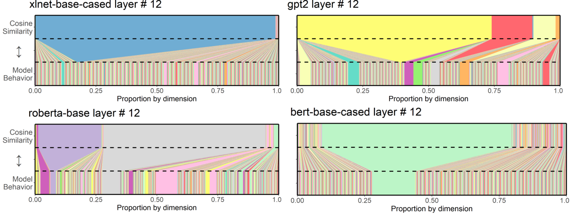
Figure 1: Relative contribution of each dimension to cosine similarity, ${CC}(f^{i}_{\ell})$, (top) paired with its relative influence on model behavior, $I(i,\ell,f)$ (bottom). The top and bottom portions of the plots each have 768 bars, one for each dimension in layer 12. The width of the bars corresponds to their relative contribution to each metric. For example, three dimensions (yellow, red, light yellow) dominate cosine similarity in GPT-2, but when we trace those dimensions to the bottom half of the plot, they appear to vanish, meaning their relative influence on model behavior is negligible. While this mismatch is less pronounced for BERT, it is particularly extreme in XLNet, where a single dimension dominates cosine similarity, but is effectively meaningless to the pretraining objective.

4 Rogue Dimensions and Model Behavior

In this section, we address the question of whether the dimensions which dominate cosine similarity likewise dominate model behavior. Specifically, if similarity measures are dominated by only a few dimensions, as shown in the previous sections, then those dimensions should be the only ones the model actually uses, otherwise, the measures only reflect a small subset of what the model is doing. We find that dimensions which dominate cosine similarity do not likewise dominate model behavior.

4.1 Behavioral Influence of Individual Dimensions

We measure the influence of individual dimensions on model behavior through an ablation study in the style of Morcos et al. (2018). The idea of neuron ablation studies is to examine how the performance of a network changes when a neuron is clamped to a fixed value, typically zero. In our study, we measure how much the language modeling distribution changes when dimension $i$ of layer $\ell$ is fixed to zero.

4.2 Setup

Let $P_{f}(s)$ be the original language modeling distribution of model $f$ for some input $s$ sampled from corpus $\mathcal{O}$. We measure how the distribution changes after ablation using KL divergence between the ablated model distribution and the unaltered reference distribution. We use KL divergence, rather than typical measures of importance in feature ablation such as accuracy or perplexity because we are interested in how much the prediction distributions change rather than performance on some task. Our measure of the importance of dimension $i$ in layer $\ell$ of model $f$ is the mean KL divergence between the two distributions across our corpus, where $S$ is a set of $n$ inputs to the model.

$$\begin{split}I(i,\ell,f)&=\frac{1}{n}\sum_{s\in S}^{n}D_{KL}[P_{f}(s)\rVert P_{f}(s|f^{i}_{\ell}(s)=0)]\end{split}$$ (6)

4.3 Experiment

To measure the importance of each dimension to model behavior, we compute $I(i,\ell,f)$ for the last 4 layers of each model over 10k distributions. Since the autoregressive models (GPT-2, XLNet) give a language modeling distribution over all tokens in the input, we use a corpus of 10k tokens from English Wikipedia. In the auto-encoder models (BERT, RoBERTa), we mask 15% of tokens and use a corpus of 150k tokens, for a total of 10k language modeling distributions. We plot the relative behavioral influence of each dimension against its contribution to cosine similarity, measured by ${CC}(f^{i}_{\ell})$, (each is normalized to sum to 1).

4.4 Results

Figure 1 displays the results for the final layer of each model. In all models, we see that the dimensions which dominate cosine similarity do not likewise dominate model behavior. The mismatch is less drastic in BERT’s final layer, but is quite severe in final XLNet and GPT-2, where removing the dimensions which dominate cosine similarity does not lead to substantial changes in the language modeling distribution.

While ablating rogue dimensions often alters the language modeling distribution more than ablating non-rogue dimensions, we emphasize that there is not a one-to-one correspondence between a dimension’s influence on cosine similarity and its influence on language modeling behavior. In the case of XLNet and GPT-2, removing dimensions which dominate cosine similarity leads to only vanishingly small changes to the behavior of the model.

4.5 Behavioral Correlates of Rogue Dimensions

We now turn to the related question of whether rogue dimensions actually capture linguistically meaningful information. Because rogue dimensions dominate representational similarity measures, these measures will be heavily biased toward whatever information these dimensions capture. To explore their behavioral correlates, we plotted the distribution of the values for rogue dimensions.

We show in Figure 2 that rogue dimensions often have highly type/position specific activation patterns. Rogue dimensions in all models are particularly sensitive to instances of the "." token and/or position 0 of the input. For example, in laters 2-11 of GPT-2 and RoBERTa, the mean cosine similarity of any two tokens in position 0 is greater than .99, while the mean similarity of tokens not in position 0 is .623 and .564 respectively.

While the transformer language models we have tested have all been shown to capture a rich range of linguistic phenomena, this linguistic knowledge may be obscured by rogue dimensions. The following section empirically evaluates this hypothesis.

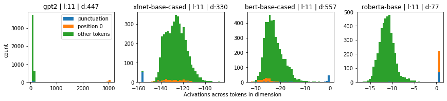
Figure 2: Distribution of values in the dimension with the highest variance in layer 11 of each model across a sample of 10k tokens from English Wikipedia. Each color corresponds to a specific type/position. The orange distribution is tokens which occur in position zero, the blue distribution is instances of the "." token, and green is instances of all other tokens. Results for all layers can be found in Figures 8 and 9 of the appendix.

5 Postprocessing and Representational Quality

While we have shown that the representational geometry of contextualized embeddings makes cosine similarity uninformative, there are several simple postprocessing methods which can correct for this. In this section we outline three such methods: standardization, all-but-the-top Mu and Viswanath (2018), and ranking (via Spearman correlation). We evaluate representational quality of the postprocessed embeddings on several word similarity/relatedness datasets and show that the underlying representational quality is obscured by the rogue dimensions. When we correct for rogue dimensions, correlation with human similarity judgments improves across the board. We also find that representational quality is preserved across all layers, rather than giving way to degraded/task specific representations as argued in previous work.

5.1 Postprocessing

Standardization: We have observed that a small subset of dimensions with means far from zero and high variance completely dominate cosine similarity. A straightforward way to adjust for this is to subtract the mean vector and divide each dimension by its standard deviation, such that each dimension has $\mu_{i}=0$ and $\sigma_{i}=1$. Concretely, given some corpus of length $|\mathcal{O}|$ containing word representations $x\in\mathbb{R}^{d}$, we compute the mean vector $\mu\in\mathbb{R}^{d}$

$$\mu=\frac{1}{|\mathcal{O}|}\cdot\sum_{x\in\mathcal{O}}x$$ (7)

as well as the standard deviation in each dimension $\sigma\in\mathbb{R}^{d}$

$$\sigma=\sqrt{\frac{1}{|\mathcal{O}|}\cdot\sum_{x\in\mathcal{O}}(x-\mu)^{2}}$$ (8)

Our new standardized representation for each word vector ($z$) becomes the z-score in each dimension.

$$z=\frac{x-\mu}{\sigma}$$ (9)

All-but-the-top: Following from similar observations (a nonzero common mean vector and a small number of dominant directions) in static embedding models, Mu and Viswanath (2018) proposed subtracting the common mean vector and eliminating the top few principle components (they suggested the top $\frac{d}{100}$), which should capture the variance of the rogue dimensions in the model and make the space more isotropic.

Spearman’s $\rho$: Zhelezniak et al. (2019) treat word embeddings as $d$ observations from an $|\mathcal{O}|$-variate distribution, and use Pearson correlation as a measure of similarity. They propose the use of non-parametric rank correlation coefficients, such as Spearman’s $\rho$ when embeddings depart from normality. Spearman correlation is just Pearson correlation but between the ranks of embeddings, rather than their values. Thus Spearman correlation can also be thought of as a postprocessing technique, where instead of standardizing the space or removing the top components, we simply transform embeddings as $x^{\prime}=\textit{rank(x)}$. Spearman’s $\rho$ is robust to outliers and thus will not be dominated by the rogue dimensions of contextual language models. Unlike standardization and all-but-the-top, Spearman correlation requires no computations over the entire corpus. While rank-based similarity measures will not be dominated by rogue dimensions, rogue dimensions will tend to occupy the top or bottom ranks.

5.2 Representational Quality

While we have shown that cosine similarity is dominated by a small subset of dimensions, a remaining question is whether adjusting for these dimensions makes similarity measures more informative. In particular, we evaluate whether the cosine similarities between word pairs align more closely with human similarity judgments after post-processing. We evaluate this using 4 word similarity/relatedness judgment datasets: RG65 Rubenstein and Goodenough (1965), WS353 Agirre et al. (2009), SimLex999 Hill et al. (2015) and SimVerb3500 Gerz et al. (2016). Examples in these datasets consist of a pair of words and a corresponding similarity rating averaged over several human annotators. Because the similarity judgments were designed to evaluate static embeddings, we use the context-aggregation strategy of Bommasani et al. (2020) to produce static representations.

For each model, we report the Spearman correlation between the model similarities and human-similarity judgments, averaged across all 4 datasets. We report the correlation for cosine similarities of the original embeddings, as well as for postprocessed embeddings using four strategies: standardization, all-but-the-top (removing the top 7 components), only subtracting the mean (the step common to both strategies) and Spearman correlation.

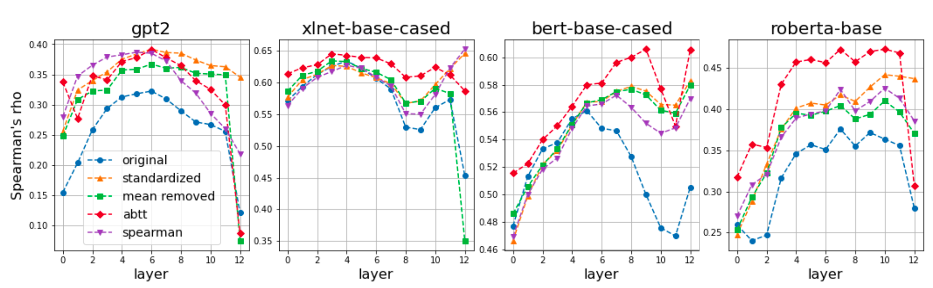
Figure 3: Average correlation (Spearman’s $\rho$) with human judgments in the four word similarity datasets, with and without postprocessing.

5.3 Results

Results are summarized in Figure 3. Our key findings are:

Postprocessing aligns the embedding space more closely to human similarity judgments across almost all layers of all models. We found that standardization was the most successful postprocessing method, showing consistent improvement over the original embeddings in all but the early layers of BERT.

All-but-the-top was generally effective, though the resulting final layer of RoBERTa and GPT-2 exhibited poor correlation with human judgements, similar to the original embeddings. In pilot analyses, we found that all-but-the-top is highly dependent on the number of components removed, a hyperparameter, $D$, which Mu and Viswanath (2018) suggest should be $\frac{d}{100}$. Just removing the first principle component in RoBERTa yielded a stronger correlation, but all-but-the top did not significantly improve correlation with human judgements in the final layer of GPT-2 for any choice of $D$.

Simply subtracting the mean vector also yielded substantial gains in most models with the exception of the final layers of GPT-2 and XLNet. The rogue dimensions in the last layer of these two models have exceptionally high variance. While subtracting the mean made the space more isotropic as measured by cosine similarity, it did not reduce the variance of each dimension. We found, particularly in the final layer of GPT-2 and XLNet that 1-3 dimensions drive the variability of cosine similarity, and this was still the case when the mean vector was subtracted.

Converting embeddings into ranks (Spearman correlation) also resulted in significantly stronger correlations with human judgments in all layers of all models, though the correlation was often weaker than standardization or all-but-the-top.

Representational quality is preserved across all layers. Previous work has suggested that the final layers of transformer language models are highly task-specific. Liu et al. (2019) showed that the middle layers of BERT outperform the final layers on language understanding tasks. Using a cosine-similarity based text-generation evaluation metric, Zhang et al. (2020) showed a sharp drop in correlation to human judgements of machine translation quality in final layers of various transformer language models. Similarly, Davis and van Schijndel (2020) used Representational Similarity Analysis (RSA) with Pearson correlation and found that intermediate layers of GPT-2 and TransformerXL encode human-like implicit causality biases which are subsequently obscured in final layers.

Our findings suggest that linguistic representational quality (in this case lexical semantics) is actually preserved in the final layers but is obscured by a small handful of rogue dimensions. After simple postprocessing, later layers of the model correlate just as well, if not better than intermediate layers with human similarity judgments. This finding reaffirms the need to carefully consider the representational geometry of a model before drawing conclusions about layerwise representational quality, and the general linguistic knowledge these models encode.

6 Discussion and Future Work

Perhaps the most important direction for future work is designing and implementing language models which do not develop rogue dimensions in the first place. Gao et al. (2019) introduce a cosine-regularization term during pretraining which improved the performance of transformer models on machine translation. Perhaps BERT or GPT models could similarly benefit from such regularization.

A prerequisite for designing models without rogue dimensions is understanding how these dimensions arise over time. Contemporaneous work from Biś et al. (2021) provides a useful characterization of how degenerate representations may be learned, which largely focuses on token frequency, while Kovaleva et al. (2021) provide a characterization of how outliers impact model performance, attributing much of the problem to scaling factors in layer normalization, and Luo et al. (2021) make observations about the contribution of positional embeddings. In the present work, we observe strong correlations with specific tokens and positions. Unifying these accounts is an important task for future work. With the recent release of the MultiBERT checkpoints Sellam et al. (2021), future work can uncover whether rogue dimensions are a coincidental property of some models, or whether they are a requisite for good performance. The MultiBERTs may also elucidate how these dimensions emerge during pretraining. While we empirically motivate a trivially simple transformation which corrects for rogue dimensions, we believe the most fruitful direction for future work is to build models whose representations require no post-hoc transformations. This would result in more interpretable embedding spaces and may additionally lead to models with better performance.

7 Conclusion

In this work, we showed that similarity measures in contextual language models are largely reflective of a small number of rogue dimensions, not the entire embedding space. Consequently, a few dimensions can drastically change the conclusions we draw about the linguistic phenomena a model actually captures. We showed that the previously observed anisotropy in contextual models is essentially an artifact of rogue dimensions and is not a global property of the entire embedding space. We also showed that variability in similarity is driven by just 1-5 dimensions of the embedding space. In many cases, removing just a single dimension completely changed which token pairs were similar to one another. However, we found that model behavior was not driven by these rogue dimensions, and that these dimensions seem to handle a small subset of a model’s linguistic abilities, such as punctuation and positional information. In summary, standard similarity measures such as cosine similarity and Euclidean distance are not informative measures of how contextual language models represent and process language. We argue that measures of similarity in contextual language models must account for rogue dimensions using techniques such as standardization. These techniques should not just be viewed as avenues to improve downstream performance, but as prerequisites for any analysis involving representational similarity.

Appendix A Removing Dominant Dimensions and Representational Geometry

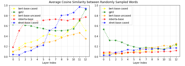
Figure 4: Anisotropy by layer of the full embedding space (left) and with the top 5 dimensions removed, as measured by $\mathbb{E}[CC_{i}]$ (right). In all models, anisotropy drastically decreases, and becomes more consistent across models and layers.

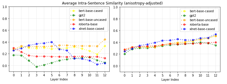
Figure 5: Intra-sentence similarity by layer of the full embedding space (left) and with the top 5 dimensions removed, as measured by $\mathbb{E}[CC_{i}]$ (right). Intra-sentence similarity is much more consistent and monotonically increasing when the top 5 dimensions are removed.

Figure 6: Average self-similarity (similarity of the same word type across contexts) by layer of the full embedding space (left) and with the top 5 dimensions removed, as measured by $\mathbb{E}[CC_{i}]$ (right). In the full embedding space, words of the same type in GPT-2 and XLNet appear no more similar to one another than randomly-sampled tokens. When we remove just 5 dimensions, words of the same type are indeed more similar to one another than the random baseline.

To facilitate a direct comparison with anisotropy estimates of Ethayarajh (2019), we replicate the experiments of Section 4 before and after removing the top $k$ dimensions with the largest $\mathbb{E}[CC_{i}]$. For these experiments we chose $k$=5 dimensions to remove. Results for anisotropy estimates are shown in Figure 4. Three key takeaways from this analysis are:

All models tested had highly anisotropic representations, including XLNet and RoBERTa which had not been evlauated in previous work. XLNet is even more anistropic than GPT-2 in its final two layers. RoBERTa’s word representations are likewise highly anisotropic, though starting in earlier layers than in XLNet and BERT.

After removing just 5 dimensions, embeddings become relatively isotropic, with $\textit{$\hat{A}$}(f_{\ell})$ never larger than 0.25 in any layer of any model.

Anisotropy becomes consistent across models and across layers, suggesting that the deviant dimensions that drive anisotropy are idiosyncratic and model/layer specific; we show this to indeed be the case in Section 4. By contrast, the geometry of the embedding space without rogue dimensions show similar properties across models/layers, suggesting that the similar qualities of the representational geometries of each model are obscured by these rogue dimensions.

This can additionally be seen in our replication of the intra-sentence similarity and self-similarity from Ethayarajh (2019). While they find extreme cases in which words of the same type are no more similar to one another than randomly sampled words, we find a consistently high degree of self-similarity across all layers of all models after removing 5 dimensions. This suggests that information about word identity is preserved across all layers, rather than giving way to extremely contextualized representations in the final layer, this concurs with our findings in Section 5. Together, these show that our conclusions about the geometry of contextual embedding spaces are heavily skewed by the sensitivity of cosine similarity to rogue dimensions present in each of these models.

Appendix B Informativity of Euclidean Distance

In this section, we conduct a similar analysis to Section 3.2 to see whether the variability in Euclidean distances between pairs of embeddings can be explained by Euclidean distance with the top $k$ dimensions are removed. Our methods for this analysis are identical to those of Section 3.2, except our criterion for choosing $k$ is the variance in each dimension. Results are shown in Table 3. In the extreme case of XLNet, none of the variability in Euclidean distances can be explained by Euclidean distances when a single dimension is removed. This means that Euclidean distance in this layer is effectively a measure of a single dimension.

Model	Layer	k=1	k=3	k=5
GPT-2	0	0.999	0.996	0.996
	1	0.983	0.975	0.975
	2	0.999	0.783	0.783
	3	0.992	0.257	0.257
	4	0.993	0.200	0.200
	5	0.993	0.159	0.159
	6	0.993	0.090	0.090
	7	0.992	0.037	0.037
	8	0.990	0.007	0.007
	9	0.990	0.002	0.002
	10	0.986	0.022	0.022
	11	0.971	0.974	0.974
	12	0.909	0.333	0.333
BERT	0	0.997	0.997	0.997
	1	0.994	0.993	0.993
	2	0.993	0.992	0.992
	3	0.994	0.993	0.993
	4	0.988	0.987	0.987
	5	0.992	0.991	0.991
	6	0.988	0.987	0.987
	7	0.982	0.981	0.981
	8	0.969	0.968	0.968
	9	0.925	0.924	0.924
	10	0.762	0.761	0.761
	11	0.434	0.433	0.433
	12	0.990	0.989	0.989
RoBERTa	0	0.810	0.770	0.770
	1	0.509	0.264	0.264
	2	0.584	0.141	0.141
	3	0.607	0.152	0.152
	4	0.657	0.200	0.200
	5	0.623	0.225	0.225
	6	0.641	0.242	0.242
	7	0.614	0.241	0.241
	8	0.578	0.235	0.235
	9	0.591	0.270	0.270
	10	0.575	0.281	0.281
	11	0.591	0.319	0.319
	12	0.566	0.301	0.301
XLNet	0	0.999	0.996	0.996
	1	1.000	1.000	1.000
	2	1.000	0.987	0.987
	3	0.993	0.992	0.992
	4	0.983	0.978	0.978
	5	0.903	0.896	0.896
	6	0.481	0.470	0.470
	7	0.432	0.426	0.426
	8	0.235	0.236	0.236
	9	0.321	0.323	0.323
	10	0.308	0.307	0.307
	11	0.124	0.150	0.150
	12	0.028	0.024	0.024

Table 3: Proportion of variance in Euclidean distance $r^{2}$ explained by Euclidean distance when the top $k$ dimensions (measured by the variance in each dimension) are removed.

Model	Layer	1	2	3	$\textit{$\hat{A}$}(f_{\ell})$
GPT-2	0	0.054	0.051	0.051	0.484
	1	0.324	0.163	0.150	0.626
	2	0.319	0.205	0.149	0.612
	3	0.294	0.264	0.145	0.589
	4	0.297	0.275	0.151	0.549
	5	0.324	0.258	0.150	0.517
	6	0.351	0.237	0.148	0.485
	7	0.374	0.205	0.144	0.466
	8	0.376	0.156	0.141	0.461
	9	0.364	0.190	0.157	0.466
	10	0.326	0.257	0.207	0.498
	11	0.275	0.269	0.265	0.640
	12	0.763	0.131	0.078	0.885
BERT	0	0.159	0.076	0.035	0.066
	1	0.541	0.049	0.024	0.154
	2	0.790	0.006	0.005	0.224
	3	0.792	0.006	0.004	0.234
	4	0.781	0.007	0.005	0.283
	5	0.809	0.007	0.005	0.360
	6	0.792	0.005	0.004	0.382
	7	0.716	0.006	0.005	0.342
	8	0.668	0.006	0.006	0.326
	9	0.743	0.004	0.004	0.380
	10	0.817	0.004	0.003	0.396
	11	0.884	0.003	0.002	0.506
	12	0.686	0.005	0.005	0.370
RoBERTa	0	0.726	0.040	0.021	0.143
	1	0.850	0.081	0.009	0.442
	2	0.862	0.093	0.013	0.627
	3	0.841	0.113	0.017	0.659
	4	0.796	0.146	0.023	0.666
	5	0.775	0.160	0.025	0.672
	6	0.745	0.180	0.030	0.679
	7	0.726	0.193	0.032	0.705
	8	0.674	0.229	0.038	0.690
	9	0.648	0.254	0.040	0.675
	10	0.698	0.223	0.032	0.689
	11	0.666	0.252	0.031	0.696
	12	0.663	0.262	0.020	0.745
XLNet	0	0.300	0.043	0.028	0.037
	1	0.085	0.059	0.036	0.022
	2	0.042	0.031	0.016	0.050
	3	0.157	0.013	0.011	0.051
	4	0.413	0.017	0.009	0.169
	5	0.700	0.005	0.004	0.177
	6	0.908	0.003	0.002	0.514
	7	0.942	0.001	0.001	0.563
	8	0.982	0.000	0.000	0.826
	9	0.984	0.000	0.000	0.833
	10	0.990	0.000	0.000	0.887
	11	0.996	0.001	0.000	0.981
	12	0.973	0.003	0.002	0.884

Table 4: Proportion of total expected cosine similarity, ${CC}(f^{i}_{\ell})/\textit{$\hat{A}$}(f_{\ell})$, contributed by each of the top 3 dimensions for all layers of each model, along with the anisotropy estimate $\textit{$\hat{A}$}(f_{\ell})$ for the given layer.

Model	Layer	k=1	k=3	k=5
GPT-2	0	0.999	0.996	0.996
	1	0.985	0.888	0.888
	2	0.990	0.899	0.899
	3	0.991	0.849	0.849
	4	0.910	0.775	0.775
	5	0.872	0.719	0.719
	6	0.853	0.684	0.684
	7	0.862	0.713	0.713
	8	0.894	0.797	0.797
	9	0.921	0.490	0.490
	10	0.947	0.428	0.428
	11	0.967	0.352	0.352
	12	0.819	0.232	0.232
BERT	0	0.999	0.997	0.997
	1	0.894	0.848	0.848
	2	0.580	0.568	0.568
	3	0.514	0.504	0.504
	4	0.459	0.449	0.449
	5	0.383	0.374	0.374
	6	0.343	0.338	0.338
	7	0.391	0.394	0.394
	8	0.400	0.398	0.398
	9	0.219	0.220	0.220
	10	0.119	0.123	0.123
	11	0.046	0.048	0.048
	12	0.213	0.214	0.214
RoBERTa	0	0.810	0.770	0.770
	1	0.509	0.264	0.264
	2	0.584	0.141	0.141
	3	0.607	0.152	0.152
	4	0.657	0.200	0.200
	5	0.623	0.225	0.225
	6	0.641	0.242	0.242
	7	0.614	0.241	0.241
	8	0.578	0.235	0.235
	9	0.591	0.270	0.270
	10	0.575	0.281	0.281
	11	0.591	0.319	0.319
	12	0.566	0.301	0.301
XLNet	0	0.999	0.996	0.996
	1	1.000	1.000	1.000
	2	1.000	0.987	0.987
	3	0.993	0.992	0.992
	4	0.983	0.978	0.978
	5	0.903	0.896	0.896
	6	0.481	0.470	0.470
	7	0.432	0.426	0.426
	8	0.235	0.236	0.236
	9	0.321	0.323	0.323
	10	0.308	0.307	0.307
	11	0.124	0.150	0.150
	12	0.028	0.024	0.024

Table 5: Proportion of variance in cosine similarity $r^{2}$ explained by cosine similarity when the top $k$ dimensions (measured by cosine similarity contribution) are removed. Layer 0 is the static embedding layer.

   

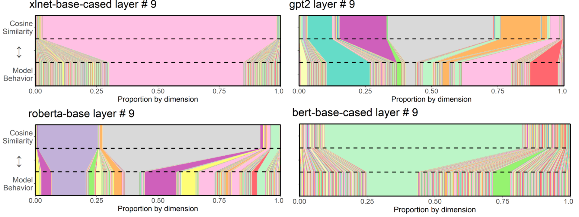
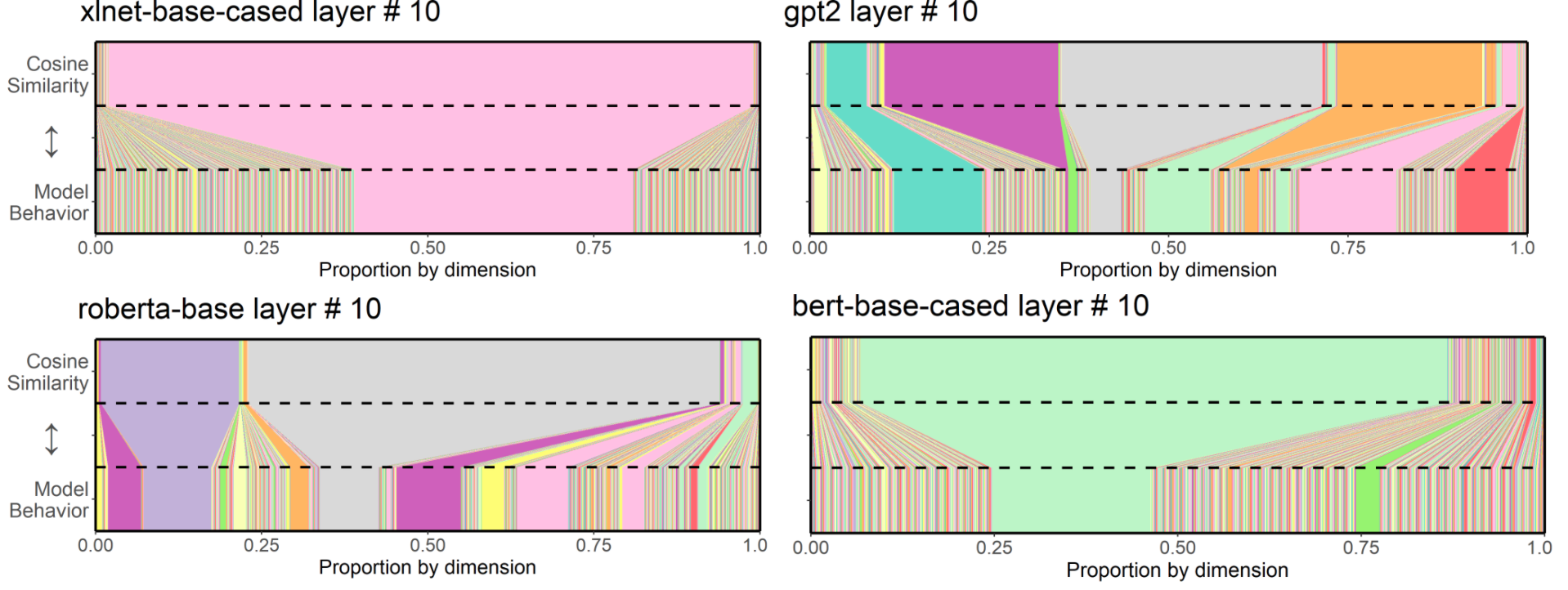
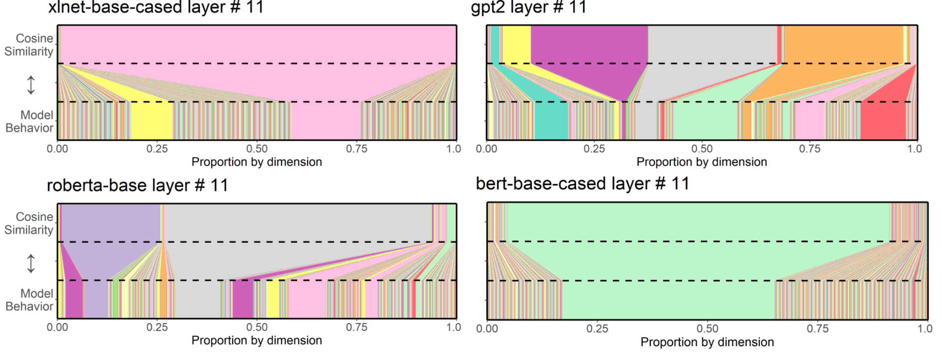
Figure 7: Relative contribution of each dimension to cosine similarity (top) paired with its relative influence on model behavior (bottom) for layers 9-11 of each model.

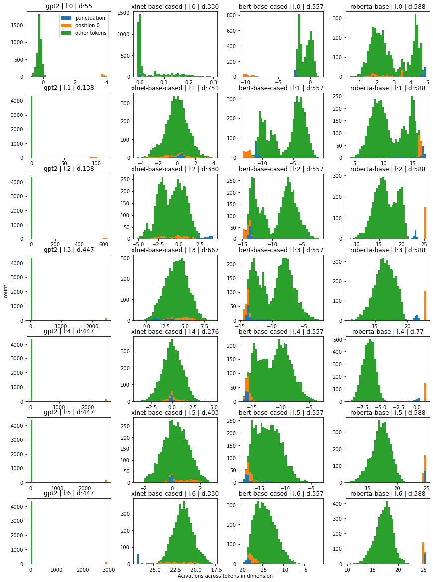
Figure 8: Distribution of activations in the dimension with highest variance in layers 0-6 of each model across a sample of 10k tokens. Each color corresponds to a specific type/position, where the orange distribution is tokens occurring in position zero, the blue distribution is instances of the "." token, and green is all other tokens. In many cases, there are two clear modes in each distribution, where one corresponds to a specific word type or position. Additionally, this behavior tends to persist within the same dimension number across layers, which is facilitated by the residual connections present in each model.

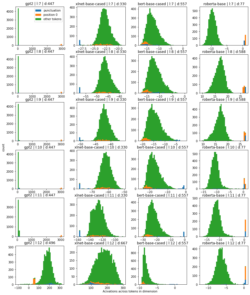
Figure 9: Distribution of activations in the dimension with highest variance in layers 7-12 of each model across a sample of 10k tokens. Each color corresponds to a specific type/position, where the orange distribution is tokens occurring in position zero, the blue distribution is instances of the "." token, and green is all other tokens. In many cases, there are two clear modes in each distribution, where one corresponds to a specific word type or position. Additionally, this behavior tends to persist within the same dimension number across layers, which is facilitated by the residual connections present in each model.

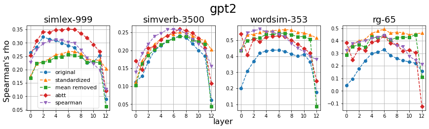
Figure 10: Average correlation (Spearman’s $\rho$) with human judgements on each word similarity dataset, with and without postprocessing for GPT-2

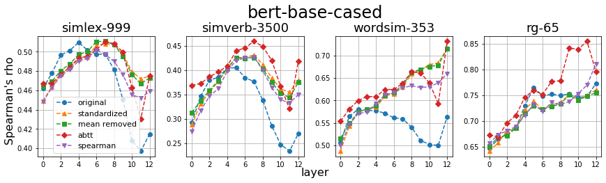
Figure 11: Average correlation (Spearman’s $\rho$) with human judgements on each word similarity dataset, with and without postprocessing for BERT

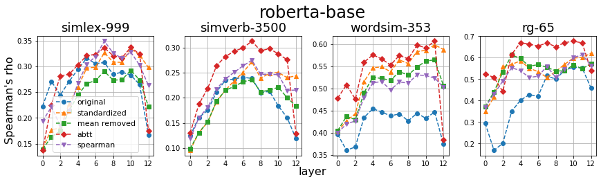
Figure 12: Average correlation (Spearman’s $\rho$) with human judgements on each word similarity dataset, with and without postprocessing for RoBERTa

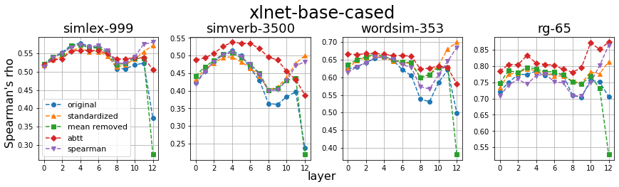
Figure 13: Average correlation (Spearman’s $\rho$) with human judgements on each word similarity dataset, with and without postprocessing for XLNet

References

- A. Rodriguez and Merlo (2020) Maria A. Rodriguez and Paola Merlo. 2020. Word associations and the distance properties of context-aware word embeddings. In Proceedings of the 24th Conference on Computational Natural Language Learning, pages 376–385, Online. Association for Computational Linguistics.
- Abnar et al. (2019) Samira Abnar, Lisa Beinborn, Rochelle Choenni, and Willem Zuidema. 2019. Blackbox meets blackbox: Representational similarity & stability analysis of neural language models and brains. In Proceedings of the 2019 ACL Workshop BlackboxNLP: Analyzing and Interpreting Neural Networks for NLP, pages 191–203, Florence, Italy. Association for Computational Linguistics.
- Agirre et al. (2009) Eneko Agirre, Enrique Alfonseca, Keith Hall, Jana Kravalova, Marius Paşca, and Aitor Soroa. 2009. A study on similarity and relatedness using distributional and WordNet-based approaches. In Proceedings of Human Language Technologies: The 2009 Annual Conference of the North American Chapter of the Association for Computational Linguistics, pages 19–27, Boulder, Colorado. Association for Computational Linguistics.
- Bach et al. (2015) Sebastian Bach, Alexander Binder, Grégoire Montavon, Frederick Klauschen, Klaus-Robert Müller, and Wojciech Samek. 2015. On pixel-wise explanations for non-linear classifier decisions by layer-wise relevance propagation. PLOS ONE, 10(7):1–46.
- Baroni et al. (2014) Marco Baroni, Georgiana Dinu, and Germán Kruszewski. 2014. Don’t count, predict! a systematic comparison of context-counting vs. context-predicting semantic vectors. In Proceedings of the 52nd Annual Meeting of the Association for Computational Linguistics (Volume 1: Long Papers), pages 238–247, Baltimore, Maryland. Association for Computational Linguistics.
- Biś et al. (2021) Daniel Biś, Maksim Podkorytov, and Xiuwen Liu. 2021. Too much in common: Shifting of embeddings in transformer language models and its implications. In Proceedings of the 2021 Conference of the North American Chapter of the Association for Computational Linguistics: Human Language Technologies, pages 5117–5130, Online. Association for Computational Linguistics.
- Bommasani et al. (2020) Rishi Bommasani, Kelly Davis, and Claire Cardie. 2020. Interpreting Pretrained Contextualized Representations via Reductions to Static Embeddings. In Proceedings of the 58th Annual Meeting of the Association for Computational Linguistics, pages 4758–4781, Online. Association for Computational Linguistics.
- Cai et al. (2021) Xingyu Cai, Jiaji Huang, Yuchen Bian, and Kenneth Church. 2021. Isotropy in the contextual embedding space: Clusters and manifolds. In International Conference on Learning Representations.
- Chronis and Erk (2020) Gabriella Chronis and Katrin Erk. 2020. When is a bishop not like a rook? when it’s like a rabbi! multi-prototype BERT embeddings for estimating semantic relationships. In Proceedings of the 24th Conference on Computational Natural Language Learning, pages 227–244, Online. Association for Computational Linguistics.
- Chrupała and Alishahi (2019) Grzegorz Chrupała and Afra Alishahi. 2019. Correlating neural and symbolic representations of language. In Proceedings of the 57th Annual Meeting of the Association for Computational Linguistics, pages 2952–2962, Florence, Italy. Association for Computational Linguistics.
- Davis and van Schijndel (2020) Forrest Davis and Marten van Schijndel. 2020. Discourse structure interacts with reference but not syntax in neural language models. In Proceedings of the 24th Conference on Computational Natural Language Learning, pages 396–407, Online. Association for Computational Linguistics.
- Devlin et al. (2019) Jacob Devlin, Ming-Wei Chang, Kenton Lee, and Kristina Toutanova. 2019. BERT: Pre-training of deep bidirectional transformers for language understanding. In Proceedings of the 2019 Conference of the North American Chapter of the Association for Computational Linguistics: Human Language Technologies, Volume 1 (Long and Short Papers), pages 4171–4186, Minneapolis, Minnesota. Association for Computational Linguistics.
- Ethayarajh (2019) Kawin Ethayarajh. 2019. How contextual are contextualized word representations? Comparing the geometry of BERT, ELMo, and GPT-2 embeddings. In Proceedings of the 2019 Conference on Empirical Methods in Natural Language Processing and the 9th International Joint Conference on Natural Language Processing (EMNLP-IJCNLP), pages 55–65, Hong Kong, China. Association for Computational Linguistics.
- Gao et al. (2019) Jun Gao, Di He, Xu Tan, Tao Qin, Liwei Wang, and Tieyan Liu. 2019. Representation degeneration problem in training natural language generation models. In International Conference on Learning Representations.
- Garcia et al. (2021) Marcos Garcia, Tiago Kramer Vieira, Carolina Scarton, Marco Idiart, and Aline Villavicencio. 2021. Probing for idiomaticity in vector space models. In Proceedings of the 16th Conference of the European Chapter of the Association for Computational Linguistics: Main Volume, pages 3551–3564, Online. Association for Computational Linguistics.
- Gerz et al. (2016) Daniela Gerz, Ivan Vulić, Felix Hill, Roi Reichart, and Anna Korhonen. 2016. SimVerb-3500: A large-scale evaluation set of verb similarity. In Proceedings of the 2016 Conference on Empirical Methods in Natural Language Processing, pages 2173–2182, Austin, Texas. Association for Computational Linguistics.
- Hill et al. (2015) Felix Hill, Roi Reichart, and Anna Korhonen. 2015. SimLex-999: Evaluating semantic models with (genuine) similarity estimation. Computational Linguistics, 41(4):665–695.
- Kovaleva et al. (2021) Olga Kovaleva, Saurabh Kulshreshtha, Anna Rogers, and Anna Rumshisky. 2021. BERT busters: Outlier dimensions that disrupt transformers. In Findings of the Association for Computational Linguistics: ACL-IJCNLP 2021, pages 3392–3405, Online. Association for Computational Linguistics.
- Li et al. (2020) Bohan Li, Hao Zhou, Junxian He, Mingxuan Wang, Yiming Yang, and Lei Li. 2020. On the sentence embeddings from pre-trained language models. In Proceedings of the 2020 Conference on Empirical Methods in Natural Language Processing (EMNLP), pages 9119–9130, Online. Association for Computational Linguistics.
- Liu et al. (2019) Nelson F. Liu, Matt Gardner, Yonatan Belinkov, Matthew E. Peters, and Noah A. Smith. 2019. Linguistic knowledge and transferability of contextual representations. In Proceedings of the 2019 Conference of the North American Chapter of the Association for Computational Linguistics: Human Language Technologies, Volume 1 (Long and Short Papers), pages 1073–1094, Minneapolis, Minnesota. Association for Computational Linguistics.
- Liu et al. (2020) Yinhan Liu, Myle Ott, Naman Goyal, Jingfei Du, Mandar Joshi, Danqi Chen, Omer Levy, Mike Lewis, Luke Zettlemoyer, and Veselin Stoyanov. 2020. Roberta: A robustly optimized bert pretraining approach.
- Luo et al. (2021) Ziyang Luo, Artur Kulmizev, and Xiaoxi Mao. 2021. Positional artefacts propagate through masked language model embeddings. In Proceedings of the 59th Annual Meeting of the Association for Computational Linguistics and the 11th International Joint Conference on Natural Language Processing (Volume 1: Long Papers), pages 5312–5327, Online. Association for Computational Linguistics.
- Martinc et al. (2020) Matej Martinc, Petra Kralj Novak, and Senja Pollak. 2020. Leveraging contextual embeddings for detecting diachronic semantic shift. In Proceedings of the 12th Language Resources and Evaluation Conference, pages 4811–4819, Marseille, France. European Language Resources Association.
- May et al. (2019) Chandler May, Alex Wang, Shikha Bordia, Samuel R. Bowman, and Rachel Rudinger. 2019. On measuring social biases in sentence encoders. In Proceedings of the 2019 Conference of the North American Chapter of the Association for Computational Linguistics: Human Language Technologies, Volume 1 (Long and Short Papers), pages 622–628, Minneapolis, Minnesota. Association for Computational Linguistics.
- Merchant et al. (2020) Amil Merchant, Elahe Rahimtoroghi, Ellie Pavlick, and Ian Tenney. 2020. What happens to BERT embeddings during fine-tuning? In Proceedings of the Third BlackboxNLP Workshop on Analyzing and Interpreting Neural Networks for NLP, pages 33–44, Online. Association for Computational Linguistics.
- Mickus et al. (2020) Timothee Mickus, Denis Paperno, Mathieu Constant, and Kees van Deemter. 2020. What do you mean, BERT? In Proceedings of the Society for Computation in Linguistics 2020, pages 279–290, New York, New York. Association for Computational Linguistics.
- Mikolov et al. (2013) Tomas Mikolov, Ilya Sutskever, Kai Chen, Greg S Corrado, and Jeff Dean. 2013. Distributed representations of words and phrases and their compositionality. In Advances in Neural Information Processing Systems, volume 26. Curran Associates, Inc.
- Morcos et al. (2018) Ari S. Morcos, David G.T. Barrett, Neil C. Rabinowitz, and Matthew Botvinick. 2018. On the importance of single directions for generalization. In International Conference on Learning Representations.
- Mu and Viswanath (2018) Jiaqi Mu and Pramod Viswanath. 2018. All-but-the-top: Simple and effective postprocessing for word representations. In International Conference on Learning Representations.
- Pennington et al. (2014) Jeffrey Pennington, Richard Socher, and Christopher Manning. 2014. GloVe: Global vectors for word representation. In Proceedings of the 2014 Conference on Empirical Methods in Natural Language Processing (EMNLP), pages 1532–1543, Doha, Qatar. Association for Computational Linguistics.
- Radford et al. (2019) A. Radford, Jeffrey Wu, R. Child, David Luan, Dario Amodei, and Ilya Sutskever. 2019. Language models are unsupervised multitask learners.
- Reif et al. (2019) Emily Reif, Ann Yuan, Martin Wattenberg, Fernanda B Viegas, Andy Coenen, Adam Pearce, and Been Kim. 2019. Visualizing and measuring the geometry of bert. In Advances in Neural Information Processing Systems, volume 32. Curran Associates, Inc.
- Rubenstein and Goodenough (1965) Herbert Rubenstein and John B. Goodenough. 1965. Contextual correlates of synonymy. Commun. ACM, 8(10):627–633.
- Schnabel et al. (2015) Tobias Schnabel, Igor Labutov, David Mimno, and Thorsten Joachims. 2015. Evaluation methods for unsupervised word embeddings. In Proceedings of the 2015 Conference on Empirical Methods in Natural Language Processing, pages 298–307, Lisbon, Portugal. Association for Computational Linguistics.
- Sellam et al. (2021) Thibault Sellam, Steve Yadlowsky, Jason Wei, Naomi Saphra, Alexander D’Amour, Tal Linzen, Jasmijn Bastings, Iulia Turc, Jacob Eisenstein, Dipanjan Das, Ian Tenney, and Ellie Pavlick. 2021. The multiberts: Bert reproductions for robustness analysis.
- Soler and Apidianaki (2021) Aina Garí Soler and Marianna Apidianaki. 2021. Let’s play mono-poly: Bert can reveal words’ polysemy level and partitionability into senses.
- Vaswani et al. (2017) Ashish Vaswani, Noam Shazeer, Niki Parmar, Jakob Uszkoreit, Llion Jones, Aidan N. Gomez, Lukasz Kaiser, and Illia Polosukhin. 2017. Attention is all you need. CoRR, abs/1706.03762.
- Voita et al. (2020) Elena Voita, Rico Sennrich, and Ivan Titov. 2020. Analyzing the source and target contributions to predictions in neural machine translation.
- Vulić et al. (2020) Ivan Vulić, Edoardo Maria Ponti, Robert Litschko, Goran Glavaš, and Anna Korhonen. 2020. Probing pretrained language models for lexical semantics. In Proceedings of the 2020 Conference on Empirical Methods in Natural Language Processing (EMNLP), pages 7222–7240, Online. Association for Computational Linguistics.
- Wang et al. (2019) Bin Wang, Angela Wang, Fenxiao Chen, Yuncheng Wang, and C.-C. Jay Kuo. 2019. Evaluating word embedding models: methods and experimental results. APSIPA Transactions on Signal and Information Processing, 8.
- Yang et al. (2019) Zhilin Yang, Zihang Dai, Yiming Yang, Jaime Carbonell, Russ R Salakhutdinov, and Quoc V Le. 2019. Xlnet: Generalized autoregressive pretraining for language understanding. In Advances in Neural Information Processing Systems, volume 32. Curran Associates, Inc.
- Zhang et al. (2020) Tianyi Zhang, Varsha Kishore, Felix Wu, Kilian Q. Weinberger, and Yoav Artzi. 2020. Bertscore: Evaluating text generation with bert. In International Conference on Learning Representations.
- Zhelezniak et al. (2019) Vitalii Zhelezniak, Aleksandar Savkov, April Shen, and Nils Hammerla. 2019. Correlation coefficients and semantic textual similarity. In Proceedings of the 2019 Conference of the North American Chapter of the Association for Computational Linguistics: Human Language Technologies, Volume 1 (Long and Short Papers), pages 951–962, Minneapolis, Minnesota. Association for Computational Linguistics.