Nonuniform mixing

Abstract

Fluid mixing usually involves the interplay between advection and diffusion, which together cause any initial distribution of passive scalar to homogenize and ultimately reach a uniform state. However, this scenario only holds when the velocity field is nondivergent and has no normal component to the boundary. If either condition is unmet, such as for active particles in a bounded region, floating particles, or for filters, then the ultimate state after a long time is not uniform, and may be time dependent. We show that in those cases of nonuniform mixing it is preferable to characterize the degree of mixing in terms of an $f$-divergence, which is a generalization of relative entropy, or to use the $L^{1}$ norm. Unlike concentration variance ($L^{2}$ norm), the $f$-divergence and $L^{1}$ norm always decay monotonically, even for nonuniform mixing, which facilitates measuring the rate of mixing. We show by an example that flows that mix well for the nonuniform case can be drastically different from efficient uniformly mixing flows.

I Introduction

I.1 Uniform mixing

The standard paradigm for mixing in fluids is as follows [1, 2, 3, 4, 5]. Initially, some passive scalar (such as red dye or virus particles) is inhomogeneously distributed in a fluid. Given enough time, the dye would diffuse and spread uniformly throughout the domain; stirring the fluid greatly enhances the speed of this homogenization process. The ultimate steady state is a fluid with uniform concentration of dye throughout the domain.

The mathematical underpinning for this process is straightforward. The dye concentration $\theta(\bm{x},t)$ obeys the advection-diffusion equation

$$\partial_{t}\theta+\bm{u}\cdot\nabla\theta=D\,\nabla^{2}\theta$$ (I.1)

where the velocity field $\bm{u}(\bm{x},t)$ is nondivergent ($\nabla\cdot\bm{u}=0$), and $D>0$ is the dye diffusivity. Since a constant $\theta$ solves (I.1), we can assume without loss of generality that $\int_{\Omega}\theta\mathop{}\!\mathrm{d}{V}=0$, that is, $\theta$ has zero mean over the bounded domain $\Omega$. In that case we find after a few integrations by parts

$$\frac{\mathrm{d}}{\mathrm{d}{t}}\int_{\Omega}\theta^{2}\mathop{}\!\mathrm{d}{V}=-2D\int_{\Omega}\lvert\nabla\theta\rvert^{2}\mathop{}\!\mathrm{d}{V}\leq 0,$$ (I.2)

where boundary terms vanish, assuming no-flux boundary conditions on $\theta$. Equation I.2 gives the evolution of the concentration variance or $L^{2}$ norm of $\theta$, and the nonpositivity of the right-hand side shows that variance will decrease until $\theta$ is a constant throughout the whole domain $\Omega$. This constant vanishes because of the zero-mean assumption, so the ultimate steady state is $\theta\equiv 0$ everywhere. We then declare the dye to be mixed. This argument makes no reference to the velocity $\bm{u}(\bm{x},t)$, since the terms involving it have integrated away. Equation I.2 thus cannot be used to get a useful estimate of the rate of mixing. Nevertheless, simply having an equation such as (I.2) is essential in mathematical analysis since it guarantees mixing for long enough times, no matter what the form of $\bm{u}$. It also validates the common use of variance as a measure of the degree of mixing. The right-hand side of Eq. I.2 is called the variance dissipation, and the magnitude of its integrand is a useful proxy for regions where mixing is most active.

Figure 1: In the presence of a suction flow, passive particles such as viruses accumulate near a filter. The filter is permeable to fluid but not to particles.

I.2 Compressibility

When the fluid is compressible, the fluid density $\rho(\bm{x},t)>0$ is solved for along with the concentration $\theta(\bm{x},t)$, and instead of (I.1) we have the coupled equations

$$\partial_{t}\rho+\nabla\cdot(\bm{u}\rho)=0,\qquad\partial_{t}(\rho\,\theta)+\nabla\cdot(\bm{u}\rho\,\theta)=D\,\nabla^{2}\theta.$$ (I.3)

Notice that $\theta=\text{const.}$ is still a solution of (I.3), so the ultimate steady state remains uniform. The concentration variance equation (I.2) becomes

$$\frac{\mathrm{d}}{\mathrm{d}{t}}\int_{\Omega}\rho\,\theta^{2}\mathop{}\!\mathrm{d}{V}=-2D\int_{\Omega}\lvert\nabla\theta\rvert^{2}\mathop{}\!\mathrm{d}{V}\leq 0,$$ (I.4)

again assuming no-flux boundary conditions on $\theta$. The variance will relax to zero over time, implying that $\theta(\bm{x},t)$ reaches the uniform mixed state. In that sense compressible mixing is also an instance of a uniform mixing scenario.

Note that setting $\rho=\text{const.}$ in (I.3) necessarily implies that $\nabla\cdot\bm{u}=0$. Starting in the next section we shall allow for cases where $\nabla\cdot\bm{u}\neq 0$, but where fluid density does not enter the problem. These cases are not the same as compressible mixing; we shall usually refer to them as divergent flows to avoid confusion.

I.3 Nonuniform mixing

There was an implicit assumption when we stated that $\theta=\text{const.}$ is a steady solution of (I.1): we required $\bm{u}\cdot\hat{\bm{n}}=0$ at the boundary $\partial\Omega$. Furthermore, when $\nabla\cdot\bm{u}\neq 0$ we must modify (I.1) to read

$$\partial_{t}\theta+\nabla\cdot(\bm{u}\,\theta)=D\,\nabla^{2}\theta$$ (I.5)

to ensure that $\int_{\Omega}\theta\mathop{}\!\mathrm{d}{V}$ is conserved under no-flux boundary conditions. For $\theta=\text{const.}$ to be a steady solution of Eq. I.1 or (I.5), we require both $\bm{u}\cdot\hat{\bm{n}}=0$ at the boundary $\partial\Omega$, as well as the nondivergence condition $\nabla\cdot\bm{u}=0$. If either of these conditions is not satisfied, then the steady state is not uniform in space. In fact there may even be no steady state at all, in which case we instead refer to an ultimate state, which is reached after a long time. We will define this ultimate state more precisely later.

The no-penetration condition $\bm{u}\cdot\hat{\bm{n}}=0$ is usually quite reasonable: it says that fluid doesn’t go through the walls. But in many relevant applications the fluid can go through boundaries, even if the passive scalar cannot. We give two examples of such a situation. (Note that we will use the term ‘passive scalar’ and ‘particles’ somewhat interchangeably. We usually denote by $\theta$ a passive scalar that can have either sign, and by $p$ or $n$ a particle density that cannot be negative.)

Particle filters.

If the fluid is air and the passive scalar consists of virus particles, then a filter is a membrane that allows the passage of air but not of viruses (hopefully). This is shown schematically in Fig. 1: the virus particles naturally accumulate at the filter where $\bm{u}\cdot\hat{\bm{n}}>0$ due to the suction effect. In this type of situation the ‘mixed state’ is no longer uniform because of this accumulation.

Active particles.

A popular model for 2D self-propelled active particles (so-called Janus particles [6]) assumes that the particles move at a constant speed $U$, in a swimming direction given by an angle $\phi$ that evolves randomly with time [7, 8]. The probability density of particles $p(\bm{x},\phi,t)$ obeys a Fokker–Planck (or Smoluchowski) equation

$$\partial_{t}p+(\bm{u}+U\hat{\bm{q}})\cdot\nabla p=D\,\nabla^{2}p+D_{\mathrm{rot}}\,\partial_{\phi}^{2}p,$$ (I.6)

with $\hat{\bm{q}}=(\cos\phi,\sin\phi)$ and rotational diffusion $D_{\mathrm{rot}}$. Equation I.6 is exactly analofous to (I.1), except that the domain $\Omega$ involves spatial coordinates $\bm{x}$ and the angle $\phi$. The fluid velocity $\bm{u}(\bm{x},t)$ obeys $\bm{u}\cdot\hat{\bm{n}}=0$ at boundaries, but the swimming velocity $U\hat{\bm{q}}$ does not: a particle may keep pushing against a boundary even after it makes contact. (It is prevented from entering the wall by the no-flux boundary condition on $p$.) Hence, the steady solution to Eq. I.6 is not uniform: particles tend to accumulate near boundaries, in a manner similar to the filter example above [9, 10, 11].

There are two other effects that can lead to nonuniform ultimate states: divergence of the velocity ($\nabla\cdot\bm{u}\neq 0$) and the presence of sources and sinks. We give examples for each case.

Divergent velocity.

Floating particles at the surface of the ocean are subjected to the fluid velocity field $\bm{u}(\bm{x},t)$ evaluated at $z=0$. Even though the three-dimensional velocity satisfies $\nabla\cdot\bm{u}=0$, the two-dimensional velocity at the surface is in general divergent. In the long-time limit, particles will tend to congregate at downwellings, where the divergence is negative. The ultimate state is thus nonuniform [12].

The same type of model applies to surfactants, which are concentration scalar fields defined at the surface of a fluid. The equation for a surfactant concentration $\theta(\bm{x},t)$ evaluated at a free surface is [13, 14]

$$\partial_{t}\theta+\nabla_{\mathrm{s}}\cdot(\bm{u}_{\mathrm{s}}\,\theta)=D\,\nabla_{\mathrm{s}}^{2}\theta-\theta\,(\nabla_{\mathrm{s}}\cdot\hat{\bm{n}}_{\mathrm{s}})\,\bm{u}\cdot\hat{\bm{n}}_{\mathrm{s}}$$ (I.7)

where $\nabla_{\mathrm{s}}$ is a gradient along the surface, $\bm{u}_{\mathrm{s}}$ is the component of $\bm{u}$ parallel to the surface, and $\hat{\bm{n}}_{\mathrm{s}}$ is the unit normal to the surface. The source-sink term on the right vanishes if the surface is flat $(\nabla_{\mathrm{s}}\cdot\hat{\bm{n}}_{\mathrm{s}}=0)$ or if it is not moving $(\bm{u}\cdot\hat{\bm{n}}_{\mathrm{s}}=0)$. Even though the three-dimensional velocity is nondivergent, the surface divergence $\nabla_{\mathrm{s}}\cdot\bm{u}_{\mathrm{s}}$ is generally nonzero. Equation I.7 thus has the form of Eq. I.5, and the surfactant concentration can achieve a nonuniform ultimate state.

Heating a room.

In the winter, a closed room may be heated by a space heater, which is a localized source of heat. A closed window somewhere else in the room may act as a sink of heat. The equilibrium state is nonuniform: after a long time, we still expect the temperature to be warmer near the heater, and cooler near the window.

Whenever Eq. I.5 fails to have a uniform steady state, we are dealing with nonuniform mixing: any initial condition $\theta(\bm{x},t_{0})$ still tends towards an ultimate state, and stirring can accelerate this convergence. However, mixing must be defined with respect to this ultimate state, not the uniform state. Note that this ultimate state may be time-dependent, which challenges our natural notion of mixing even further.

Note that even if $\bm{u}\cdot\hat{\bm{n}}\neq 0$ on the boundary $\partial\Omega$, it is still typically the case that

$$\int_{\Omega}\rho\,\bm{u}\cdot\hat{\bm{n}}\mathop{}\!\mathrm{d}{S}=0,$$ (I.8)

where $\rho$ is the fluid density. Equation I.8 is a consequence of fluid mass conservation inside $\Omega$. However, we shall not assume that Eq. I.8 is satisfied in our development, since it is unnecessary, and there are cases where fluid mass might not be conserved (for instance, if there is some external source of fluid, such as rain).

I.4 Convergence to the ultimate state

When the variance equation (I.2) is modified to allow for a nonuniform ultimate state, as described in Section I.3, we will see that it no longer implies monotonic convergence to that state, because of a nonvanishing term that is sign-indefinite. Concentration variance becomes an unreliable measure of mixing, at least from a mathematical viewpoint.

We will show that, in all cases where the ultimate state is nonuniform, the degree of mixing is better captured by a kind of entropy function, related to the relative entropy of information theory and statistical physics. This entropy function has a time evolution that is always nonincreasing, no matter the subtleties of the system, and therefore always predicts convergence to an ultimate state.

We also show that the $L^{1}$ norm of $\theta$ satisfies

$$\frac{\mathrm{d}}{\mathrm{d}{t}}\int_{\Omega}\lvert\theta\rvert\mathop{}\!\mathrm{d}{V}=-2D\int_{\{\theta=0\}}\lvert\nabla\theta\rvert\mathop{}\!\mathrm{d}{S}\leq 0$$ (I.9)

where the integral on the right is taken over the zero level set of $\theta(\cdot,t)$. Equation I.9 holds in the general case, unlike the variance equation (I.2) which depends on the nondivergence $\nabla\cdot\bm{u}=0$ and $\bm{u}\cdot\hat{\bm{n}}=0$ at the boundary $\partial\Omega$. Thus, in general the $L^{1}$ norm is preferable to the $L^{2}$ norm as a measure of mixing, as we will make evident by simple numerical examples. In fact we will show that $L^{1}$ is the only $L^{q}$ norm (with $1\leq q\leq\infty$) having this monotonic decay property.

The main point of this article is that the nondivergence condition $\nabla\cdot\bm{u}=0$ and no-penetration condition $\bm{u}\cdot\hat{\bm{n}}=0$ lead to a very special situation in that the ultimate mixed state is uniform. This is not true if either of these conditions is violated; we categorize the resulting situations as nonuniform mixing. We must then revise what we mean by the rate of mixing: instead of defining it as the rate of approach to a uniform state, it is preferable to use the rate at which any two initial states converge to each other.

Nonuniform mixing can be very different from traditional mixing. For example, we will show by an example that a constant flow can be an exceedingly good mixer in the presence of suction boundary conditions, whereas such a flow is essentially useless for traditional mixing. The reason is that with the suction conditions the flow presses particles against one wall, which leads to a rapid convergence of any two initial conditions towards each other.

The presentation in this paper is unapologetically mathematical: the aim is to give the precise underpinnings in (hopefully) an agreeable language, without the rigorous burden of function spaces. In addition, the approach presented here relies on some techniques common in the analysis of convergence in Fokker–Planck equations [15, 16, 17, 18, 19, 20, 21], which are standard in statistical physics but less well known in fluid dynamics, even though the mathematical framework is similar. One major difference is that in statistical physics one is typically less concerned with specific boundary conditions, since the independent variables are often quantities like momenta, which live in unbounded spaces. In contrast, here we shall pay particularly close attention to the role of boundary conditions. Another difference is that much of the Fokker–Planck literature involves cases where the steady state exists and is easily identified, which will not be the case here for our more complicated, time-dependent examples.

It is worth noting that entropies have been used by several authors to quantify fluid mixing; see for instance [22, 23, 24, 25, 26, 27, 28, 29, 30]. However, their approaches are usually based on measuring statistical properties, whereas here we focus directly on differential equations to get rigorous bounds. Entropy and mixing are also often studied in the context of nonequilibrium thermodynamics, but in that case there is usually an equilibrium state such as a Maxwell–Boltzmann distribution towards which the system is tending. Our description will be more general and adapted to the context of fluid mixing. Approaches based on topological entropy [31, 32, 33] are complementary but not closely related to ours, since they focus on properties of trajectories of $\bm{u}(\bm{x},t)$.

Our paper is organized as follows. In Section II we define the system and derive some basic results. We consider the simplest ‘traditional’ case of nondivergent flow with impermeable boundary conditions in Section III, and show that the time-evolution equation for variance in that case predicts convergence to a uniform state. In Section IV we relax both the nondivergence and impermeability conditions. Now the ultimate state is no longer uniform, and may not even be steady. The variance equation no longer implies convergence, due to the addition of a sign-indefinite term. We remedy this by introducing the $f$-divergence associated with two probability densities $p_{1}$ and $p_{2}$, a quantity that arises in information theory. (A special case of the $f$-divergence is the relative entropy of $p_{1}$ and $p_{2}$.) We show that the time evolution of the $f$-divergence is nondecreasing, and that it must eventually decrease to zero.

We give some simple examples for flows that can be fully solved in Section V. In particular, we show that a constant flow with suction boundary conditions can be surprisingly effective at mixing. In Section VI we incorporate the effect of sources and sinks. For those we need to slightly generalize the definition of $f$-divergence, and we can still show convergence to an ultimate state. We discuss the time evolution of the $L^{1}$ norm in Section VII. Finally, we offer some concluding remarks in Section VIII.

II A particle in a closed domain

Consider a particle in a closed, connected domain $\Omega$. The particle could represent a virus, or some molecule of a pollutant. The particle evolves according to a velocity field (or drift) $\bm{u}(\bm{x},t)$ and a diffusion tensor $\mathbb{D}(\bm{x},t)$. The probability of finding the particle in a small volume $\mathop{}\!\mathrm{d}{V}_{\bm{x}}$ centered on $\bm{x}$ is $p(\bm{x},t)\mathop{}\!\mathrm{d}{V}_{\bm{x}}$, where the probability density obeys the Fokker–Planck equation

$$\partial_{t}p+\nabla\cdot\bm{F}(p)=0,\qquad\bm{x}\in\Omega,$$ (II.1)

with the probability flux defined as

$$\bm{F}(p)\mathrel{\raisebox{0.29707pt}{:}\!\!=}\bm{u}(\bm{x},t)\,p-\mathbb{D}(\bm{x},t)\cdot\nabla p\,.$$ (II.2)

The probability flux consists of an advective part and a diffusive part. In the fluid-dynamical context Eq. II.1 is called an advection-diffusion equation.

The probability density satisfies $p\geq 0$ and $\int_{\Omega}p\mathop{}\!\mathrm{d}{V}\leq 1$. (If the total probability is less than one, then the particle might not be in the domain at all.) We can integrate Eq. II.1 over $\Omega$ and use the divergence theorem to get

$$\frac{\mathrm{d}}{\mathrm{d}{t}}\int_{\Omega}p(\bm{x},t)\mathop{}\!\mathrm{d}{V}=-\int_{\partial\Omega}\bm{F}(p)\cdot\mathop{}\!\mathrm{d}{\bm{S}}\,,$$ (II.3)

where $\mathop{}\!\mathrm{d}{\bm{S}}=\hat{\bm{n}}\mathop{}\!\mathrm{d}{S}$, with $\hat{\bm{n}}$ the outward unit normal to the boundary $\partial\Omega$. Equation II.3 makes it clear that we can conserve total probability by requiring the no-flux boundary condition

$$\bm{F}(p)\cdot\hat{\bm{n}}=0,\qquad\bm{x}\in\partial\Omega.$$ (II.4)

It is important to note that we have not made any assumptions on $\bm{u}(\bm{x},t)$, other than a bit of smoothness. In particular we did not assume $\nabla\cdot\bm{u}=0$. In addition, we did not assume $\bm{u}\cdot\hat{\bm{n}}=0$, so the boundary condition Eq. II.4 is of mixed type (i.e., a linear combination of $p$ and $\nabla p$).

We spoke of one particle in this section, but the description works equally well for $N$ noninteracting particles, with $N$ fixed, or if $p$ is a nonnegative quantity such as heat, appropriately normalized. Later in Section VI, we will introduce sources and sinks, so that $N$ will be allowed to vary.

III Nondivergent flow with impermeable boundary

We make the additional assumptions

$$\nabla\cdot\bm{u}=0,\quad \bm{x}\in\Omega,$$ (III.1a)

$$\qquad\bm{u}\cdot\hat{\bm{n}}=0,\quad \bm{x}\in\partial\Omega.$$ (III.1b)

Equation III.1a is the nondivergence condition, and Eq. III.1b is the impermeability condition. The no-flux boundary condition (II.4) reduces to $\hat{\bm{n}}\cdot\mathbb{D}\cdot\nabla p=0$.

Observe that, under conditions (III.1), Eq. II.1 with boundary conditions (II.4) has the steady solution $p=\varphi$, with

$$\varphi(\bm{x})={\lvert\Omega\rvert}^{-1},$$ (III.2)

where $\lvert\Omega\rvert$ is the volume of $\Omega$, so that $\int_{\Omega}\varphi\mathop{}\!\mathrm{d}{V}=1$. The solution $\varphi(\bm{x})={\lvert\Omega\rvert}^{-1}$ is called the uniform density on $\Omega$. Two important remarks are in order: (i) both conditions in (III.1) are necessary for Eq. III.2 to be a steady solution; (ii) Eq. III.2 is a steady solution even when $\bm{u}(\bm{x},t)$ and $\mathbb{D}(\bm{x},t)$ are explicit functions of time.

We define mixing as the tendency for any initial condition $p(\bm{x},t_{0})$ to converge to $\varphi(\bm{x})$ as $t\rightarrow\infty$. A traditional way of characterizing this convergence is to first define the anomaly

$$\theta(\bm{x},t)\mathrel{\raisebox{0.29707pt}{:}\!\!=}p(\bm{x},t)-\varphi(\bm{x})$$ (III.3)

so that $\int_{\Omega}\theta\mathop{}\!\mathrm{d}{V}=0$. The variance is then $\int_{\Omega}\theta^{2}\mathop{}\!\mathrm{d}{V}$; after a few integrations by parts, we find that it evolves according to

$$\frac{\mathrm{d}}{\mathrm{d}{t}}\int_{\Omega}\theta^{2}\mathop{}\!\mathrm{d}{V}=\int_{\Omega}\bm{u}\cdot\nabla\theta^{2}\mathop{}\!\mathrm{d}{V}-2\int_{\Omega}\nabla\theta\cdot\mathbb{D}\cdot\nabla\theta\mathop{}\!\mathrm{d}{V}.$$ (III.4)

The first integral on the right vanishes: from (III.1a) $\bm{u}\cdot\nabla\theta^{2}=\nabla\cdot(\bm{u}\theta^{2})$, followed by the divergence theorem and then (III.1b). Next we require that there exists a constant $\sigma>0$ such that

$$\bm{v}\cdot\mathbb{D}(\bm{x},t)\cdot\bm{v}\geq\sigma\lvert\bm{v}\rvert^{2}>0,\qquad\text{for all nonzero vectors {\hbox{\bm{v}}}},$$ (III.5)

i.e., the operator $\nabla\cdot(\mathbb{D}\cdot\nabla p)$ is uniformly elliptic. With (III.5), Eq. III.4 now gives

$$\frac{\mathrm{d}}{\mathrm{d}{t}}\int_{\Omega}\theta^{2}\mathop{}\!\mathrm{d}{V}\leq-2\sigma\int_{\Omega}\lvert\nabla\theta\rvert^{2}\mathop{}\!\mathrm{d}{V}\leq-2\sigma\lambda\int_{\Omega}\theta^{2}\mathop{}\!\mathrm{d}{V}$$ (III.6)

where in the last step we used the Poincaré–Wirtinger inequality $\lVert\nabla\theta\rVert_{2}^{2}\geq\lambda\,\lVert\theta\rVert_{2}^{2}$ for a mean-zero function $\theta$ . The constant $\lambda>0$ depends only on the domain $\Omega$. Grönwall’s lemma then yields the bound

$$\int_{\Omega}\theta^{2}(\bm{x},t)\mathop{}\!\mathrm{d}{V}\leq\mathrm{e}^{-2\sigma\lambda(t-t_{0})}\int_{\Omega}\theta^{2}(\bm{x},t_{0})\mathop{}\!\mathrm{d}{V}$$ (III.7)

which goes to zero as $t\rightarrow\infty$. We conclude that $\theta\rightarrow 0$, or $p\rightarrow\varphi$. Thus the ultimate fate of any initial $p(\bm{x},t_{0})$ is to be homogenized until the probability of finding the particle anywhere in $\Omega$ is uniform. The rate at which this happens is of order $2\sigma\lambda$, though this is generally an underestimate. In practice, the action of $\bm{u}(\bm{x},t)$, called stirring, amplifies gradients so that $\nabla\theta$ in Eq. III.4 can be much larger than required by the Poincaré–Wirtinger inequality. Nevertheless, Eq. III.7 is useful in that it proves that variance must converge to zero. What we have just described is the basic idea of what is traditionally meant by mixing in the fluids community.

What can happen if we violate the uniform ellipticity condition Eq. III.5? For example, consider the heat equation

$$\partial_{t}p=T^{\prime}(t)\,\nabla^{2}p$$ (III.8)

with time-dependent diffusion coefficient $D(t)=T^{\prime}(t)$. If $T^{\prime}(t)\sim t^{-\alpha}$ for large time, then the uniform ellipticity condition is violated when $\alpha>0$. We can rescale and use $T$ as a time coordinate, in which case we expect a long-time exponential decay of the form

$$p(\bm{x},t)-\lvert\Omega\rvert^{-1}\sim\mathrm{e}^{-\gamma T(t)}\,,$$ (III.9)

where $\gamma$ is the asymptotic decay rate for $T^{\prime}(t)=1$. Since $T(t)\sim t^{-\alpha+1}$, we see that $p$ will fail to converge to the uniform density for $\alpha>1$. Thus, the condition (III.5) is only sufficient: there may still be convergence to equilibrium even if it is not satisfied.

IV Divergent flow or permeable boundary

The situation described in Section III is straightforward: for any velocity field $\bm{u}(\bm{x},t)$ and diffusion tensor $\mathbb{D}(\bm{x},t)$, we can expect convergence to a uniform density as long as conditions (III.1) and (III.5) are satisfied. Now we investigate what happens when either the flow is divergent (Eq. III.1a not satisfied), or when there is suction of fluid through the boundary (Eq. III.1b not satisfied).

First consider the autonomous case where $\bm{u}(\bm{x},t)\rightarrow\bm{u}(\bm{x})$, and $\mathbb{D}(\bm{x},t)\rightarrow\mathbb{D}(\bm{x})$. Then there is an equilibrium density $\varphi(\bm{x})>0$ that satisfies

$$\nabla\cdot(\bm{u}\,\varphi-\mathbb{D}\cdot\nabla\varphi)=0,\quad\bm{x}\in\Omega;\qquad\bm{F}(\varphi)\cdot\hat{\bm{n}}=0,\quad\bm{x}\in\partial\Omega$$ (IV.1)

and is normalized: $\int_{\Omega}\varphi\mathop{}\!\mathrm{d}{V}=1$. We can then define the anomaly as we did in Eq. III.3; the only difference is that the reference state $\varphi(\bm{x})$ is no longer uniform. The variance evolution equation (III.4) is still valid, but now the first integral term on the right now longer vanishes. This term is not sign-definite: this means that we can no longer conclude from this equation alone that variance must decay. In fact, variance does eventually decay, but it might not do so monotonically. Equation III.4 alone is not enough to conclude that $p$ converges to $\varphi$.

It would be convenient, then, to have a quantity other than variance that does decay monotonically in this general case. To that end, consider the $f$-divergence of two normalized probability densities $p_{1}(\bm{x})$ and $p_{2}(\bm{x})$ [34, 35]:

$$H_{f}[p_{1},p_{2}]\mathrel{\raisebox{0.29707pt}{:}\!\!=}\int_{\Omega}p_{2}\,f(p_{1}/p_{2})\mathop{}\!\mathrm{d}{V}.$$ (IV.2)

Here $f:\mathbb{R}_{\geq 0}\rightarrow\mathbb{R}$ is an arbitrary convex function with $f(1)=0$. The $f$-divergence is nonnegative; indeed, since $p_{2}$ is a probability density, by Jensen’s inequality for the convex function $f$ we have

$$H_{f}[p_{1},p_{2}]\geq f\mathopen{}\mathclose{{}\left(\int_{\Omega}(p_{1}/p_{2})\,p_{2}\mathop{}\!\mathrm{d}{V}}\right)=f(1)=0.$$ (IV.3)

The $f$-divergence is zero if and only if $p_{1}\equiv p_{2}$; $H_{f}[p_{1},p_{2}]$ measures how different $p_{1}$ and $p_{2}$ are from each other—hence the name ‘divergence.’ The $f$-divergence is not generally a metric for probability densities, since $H_{f}[p_{1},p_{2}]\neq H_{f}[p_{2},p_{1}]$, though for certain choices of $f$ it can be made symmetric (see below).

We now further assume that $f$ is strictly convex and twice-differentiable. If each $p_{i}(\bm{x},t)$ evolves according to Eq. II.1, with no-flux boundary condition (II.4), then we show in Appendix A that

$${\dot{H_{f}\mkern-3.0mu}\mkern 3.0mu}{}[p_{1},p_{2}]=-\int_{\Omega}p_{2}\,f^{\prime\prime}(p_{1}/p_{2})\,\nabla(p_{1}/p_{2})\cdot\mathbb{D}\cdot\nabla(p_{1}/p_{2})\mathop{}\!\mathrm{d}{V}\leq 0$$ (IV.4)

since $f^{\prime\prime}>0$ for a strictly convex function. For $\mathbb{D}$ satisfying (III.5), notice that the right-hand side of (IV.4) is zero if and only if $p_{1}\equiv p_{2}$. Hence, any two solutions to $\partial_{t}p=-\nabla\cdot\bm{F}(p)$ converge to each other; in the autonomous case they converge to the fixed point $p=\varphi$.

We emphasize that Eq. IV.4 holds for any divergent flow, possibly with suction boundary conditions, with time-dependent $\bm{u}$ and $\mathbb{D}$. In that sense the $f$-divergence is a better descriptor of mixing than variance: it monotonically decreases for any flow. The evolution equation (IV.4) also suggests how to define mixing in the nonautonomous context: $p_{1}$ and $p_{2}$ converge to some ultimate state $\varphi(\bm{x},t)$, which is ‘locked’ to the time-dependence of $\bm{u}$ and $\mathbb{D}$. Thus, the main characteristic of mixing is not that it leads to a homogeneous state, but rather that it leads to a state that has completely forgotten the initial condition. This ultimate state must be unique (for connected $\Omega$), otherwise (IV.4) leads to a contradiction. Unfortunately, extracting an explicit bound on the decay rate from (IV.4) is much more challenging than it was in the case of variance in Eq. III.7, and is still a topic of ongoing research [17, 18, 19, 20].

The discussion of $H_{f}$ so far did not depend on a choice of the convex function $f$ in (IV.2), as long as it exists. A simple choice for $f$ is

$$f(u)=u\log u,\qquad f^{\prime\prime}(u)=1/u,$$ (IV.5)

which corresponds to the relative entropy or Kullback–Leibler divergence (KLD), denoted by $H_{\mathrm{KL}}(p_{1},p_{2})$ [36] :

$$H_{\mathrm{KL}}(p_{1},p_{2})=\int_{\Omega}p_{1}\log\mathopen{}\mathclose{{}\left(p_{1}/p_{2}}\right)\mathop{}\!\mathrm{d}{V}.$$ (IV.6)

The KLD can be interpreted as the amount of information lost when $p_{2}$ is used to approximate $p_{1}$. The KLD bounds the $L^{1}$ norm by Pinsker’s inequality:

$$\lVert p_{1}-p_{2}\rVert_{1}^{2}\leq 2\log 2\,H_{\mathrm{KL}}(p_{1},p_{2}).$$ (IV.7)

However, $H_{\mathrm{KL}}(p_{1},p_{2})$ is not symmetric in $p_{1}$ and $p_{2}$, and is unbounded when $p_{2}$ vanishes anywhere in $\Omega$. (We will discuss the time evolution of $\lVert p_{1}-p_{2}\rVert_{1}$ in Section VII.)

A slightly more involved choice for $f$ is

$$f(u)=\tfrac{1}{2}u\log u-\tfrac{1}{2}(1+u)\log[\tfrac{1}{2}(1+u)],\qquad f^{\prime\prime}(u)=(2u\,(1+u))^{-1},$$ (IV.8)

which leads to the Jensen–Shannon divergence (JSD), denoted by $H_{\mathrm{JS}}(p_{1},p_{2})$ [37]:

$$H_{\mathrm{JS}}(p_{1},p_{2}) =\tfrac{1}{2}\mathopen{}\mathclose{{}\left\{H_{\mathrm{KL}}(p_{1},p_{12})+H_{\mathrm{KL}}(p_{2},p_{12})}\right\}$$

$$=\tfrac{1}{2}\int_{\Omega}\mathopen{}\mathclose{{}\left\{p_{1}\log\mathopen{}\mathclose{{}\left(p_{1}/p_{12}}\right)+p_{2}\log\mathopen{}\mathclose{{}\left(p_{2}/p_{12}}\right)}\right\}\mathop{}\!\mathrm{d}{V}$$ (IV.9)

where $p_{12}\mathrel{\raisebox{0.29707pt}{:}\!\!=}\tfrac{1}{2}(p_{1}+p_{2})$. The JSD is symmetric in $p_{1}$ and $p_{2}$, and its square root is a metric. Moreover, it is bounded:

$$H_{\mathrm{JS}}(p_{1},p_{2})\leq\tfrac{1}{2}(\log 2)\,\lVert p_{1}-p_{2}\rVert_{1}\leq\log 2.$$ (IV.10)

An intuitive interpretation of the JSD is not so straightforward, and will not be needed here; see for instance [37].

One remark is in order: notice that in (IV.2) and (IV.4) there are several divisions by $p_{2}$, which should rightfully worry the reader since potentially $p_{2}$ could vanish at some points, for instance at the initial time. However, for any positive time $p_{2}$ immediately becomes strictly positive, because of diffusion. See the discussion in Arnold et al. [17, p. 161] for more careful considerations.

V One-dimensional examples

To summarize the previous sections: for a velocity field $\bm{u}(\bm{x},t)$ and diffusion tensor $\mathbb{D}(\bm{x},t)$, we seek solutions to the advection-diffusion equation (II.1) with no-flux boundary conditions (II.4). Then the possible scenarios, in increasing order of complexity, can be characterized as follows.

1. If both conditions in (III.1) hold, then the uniform density is $\varphi(\bm{x})=1/\lvert\Omega\rvert$. This is true whether or not $\bm{u}$ and $\mathbb{D}$ are explicitly time-dependent (i.e., autonomous or nonautonomous). In this case the variance evolution equation (III.4) is sufficient to directly show convergence to the uniform state.

2. If either condition in (III.1) is unsatisfied, then there are three subcategories:

   1. For $\bm{u}$ and $\mathbb{D}$ time-independent (autonomous), any initial $p(\bm{x},t_{0})$ converges to a nonuniform invariant density $\varphi(\bm{x})$.

   2. For $\bm{u}$ and $\mathbb{D}$ time-periodic with period $\tau$,

      $$\bm{u}(\bm{x},t)=\bm{u}(\bm{x},t+\tau),\qquad\mathbb{D}(\bm{x},t)=\mathbb{D}(\bm{x},t+\tau),$$ (V.1)

      any initial condition $p(\bm{x},t_{0})$ converges to a periodic limiting invariant density $\varphi(\bm{x},t)$, with $\varphi(\bm{x},t)=\varphi(\bm{x},t+\tau)$.

   3. For $\bm{u}$ and $\mathbb{D}$ time-dependent (nonautonomous), any initial condition $p(\bm{x},t_{0})$ converges to a time-dependent limiting invariant density $\varphi(\bm{x},t)$.

   In case 2 the $f$-divergence evolution equation (IV.4) can be used directly to show convergence to $\varphi(\bm{x},t)$.

Since case 1 is familiar from the traditional view of mixing, we will give explicit examples for the subcategories of case 2.

V.1 Example of case 2(a): Convergence to a nonuniform density

Consider a simple one-dimensional model where the domain $\Omega=[0,L]$, the velocity $\bm{u}=U\,\hat{\bm{x}}$, and $(\mathbb{D})_{ij}=D\,\delta_{ij}$, with $U$ and $D$ constants. Then (II.1) simplifies to

$$\partial_{t}p+U\partial_{x}p-D\,\partial_{x}^{2}p=0,\qquad 0<x<L$$ (V.2)

with no-flux boundary conditions

$$Up-D\,\partial_{x}p=0,\qquad x=0,L.$$ (V.3)

This may be regarded as a simple model of a filter: the flow is nondivergent and can pass through the membranes at $x=0$ and $L$, but particles cannot cross those membranes. Since the velocity and diffusivity are time-independent, Eq. V.2 has the invariant density

$$\varphi(x)=\frac{U}{D}\,\frac{\mathrm{e}^{Ux/D}}{\mathrm{e}^{UL/D}-1}\,.$$ (V.4)

The flow pushes particle against the boundary at $x=L$ (for $U>0$), creating a boundary layer of thickness $D/U$.

Now we solve the initial value problem for Eq. V.2. This is most generally done in terms of the Green’s function $p=P(x,t\,|\,x_{0},t_{0})=P(x,t-t_{0}\,|\,x_{0},0)$, which satisfies (V.2)–(V.3) with initial condition $P(x,t_{0}\,|\,x_{0},t_{0})=\delta(x-x_{0})$. The solution is not completely straightforward, since the PDE is not self-adjoint, but it can be obtained using Laplace transforms as

$$P(x,t\,|\,x_{0},t_{0})=\varphi(x)+\frac{D}{L^{3}}\sum_{n=1}^{\infty}\frac{\mathrm{e}^{-\gamma_{n}(t-t_{0})}}{2\gamma_{n}}\,\phi_{n}^{U}(x)\,\phi_{n}^{-U}(x_{0}),$$ (V.5)

with

$$\phi_{n}^{U}(x)=\mathrm{e}^{Ux/2D}\mathopen{}\mathclose{{}\left\{2\pi n\cos(n\pi x/L)+(\lvert U\rvert L/D)\sin(n\pi x/L)}\right\}$$ (V.6)

and decay rates

$$\gamma_{n}=D\,(\pi n/L)^{2}+U^{2}/4D.$$ (V.7)

The Green’s function is plotted in Fig. 2. The relaxation rate to the invariant density $\varphi(x)$ is given by $\gamma_{1}$, which is considerably enhanced by the constant flow $U$: the second term $U^{2}/4D$ is dominant for $UL/D>2\pi$. Thus, unlike in ‘traditional’ mixing problems, a constant velocity can accelerate mixing substantially (though for a large domain size there could be an initial transient before the concentration reaches the wall). This acceleration is due to the flow squashing the concentration field against the boundary. Superficially, this does not sound like mixing, but it is in the sense that it causes the scalar field $p(x,t)$ to quickly forget its initial condition and converge to the invariant density $\varphi(x)$.

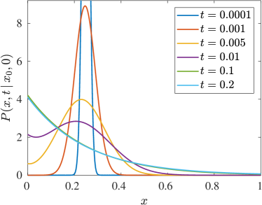
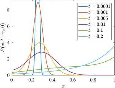
Figure 2: The Green’s function (V.5) with $x_{0}=1/4$, plotted at different times for $D=L=1$ and (a) $U=-4$; (b) $U=4$. The ultimate state is the invariant density Eq. V.4.

V.2 Example of case 2(b): Convergence to a time-periodic density

To illustrate convergence to a time-periodic invariant density $\varphi(x,t)$, we use the same system (V.2)–(V.3) as in the previous example. We mimic a time-periodic flow by reversing the direction of $\bm{u}=\pm U\,\hat{\bm{x}}$ at every half-period $\tau/2$. (This could represent the air flow reversing direction as a mask-wearer inhales and exhales.) Thus, the density $p(x,t)$ at time $t$ is evolved to time $t+\tfrac{1}{2}\tau$ by

$$p(x,t+\tfrac{1}{2}\tau) =\int_{0}^{L}P_{U}(x,\tfrac{1}{2}\tau\,|\,x_{0},0)\,p(x_{0},t)\mathop{}\!\mathrm{d}x_{0}$$ (V.8)

where $P_{U}$ is the Green’s function (V.5); then, for the next half-period, we evolve the density with a flow $\bm{u}=-U\hat{\bm{x}}$ to the left:

$$p(x,t+\tau) =\int_{0}^{L}P_{-U}(x,\tfrac{1}{2}\tau\,|\,x_{0}^{\prime},0)\,p(x_{0}^{\prime},t+\tfrac{1}{2}\tau)\mathop{}\!\mathrm{d}x_{0}^{\prime}$$

$$=\int_{0}^{L}\mathcal{P}_{\tau}(x\,|\,x_{0})\,p(x_{0},t)\mathop{}\!\mathrm{d}x_{0}$$ (V.9)

where the period-$\tau$ kernel is

$$\mathcal{P}_{\tau}(x\,|\,x_{0})\mathrel{\raisebox{0.29707pt}{:}\!\!=}\int_{0}^{L}P_{-U}(x,\tfrac{1}{2}\tau\,|\,x_{0}^{\prime},0)\,P_{U}(x_{0}^{\prime},\tfrac{1}{2}\tau\,|\,x_{0},0)\,\mathop{}\!\mathrm{d}x_{0}^{\prime}\,.$$ (V.10)

Note that $t$ in Eq. V.9 is not arbitrary but is aligned with period boundaries: $t=t_{k}=k\tau$, for integer $k$. Equation V.9 maps the density $p(x,t_{k})$ to the beginning of the next period at time $t_{k+1}=(k+1)\tau$. The invariant density $\varphi(x,t_{k})$ may be found from

$$\varphi(x,t_{k})=\int_{0}^{L}\mathcal{P}_{\tau}(x\,|\,x_{0})\,\varphi(x,t_{k})\mathop{}\!\mathrm{d}x_{0}$$ (V.11)

which is a Fredholm integral equation of the second kind. Here $\varphi(x,t_{k})$ is the periodic invariant density evaluated at the start of a period. Even for this simple time-periodic example it is not straightforward to compute $\varphi(x,t_{k})$, or the rate of convergence to $\varphi(x,t_{k})$.

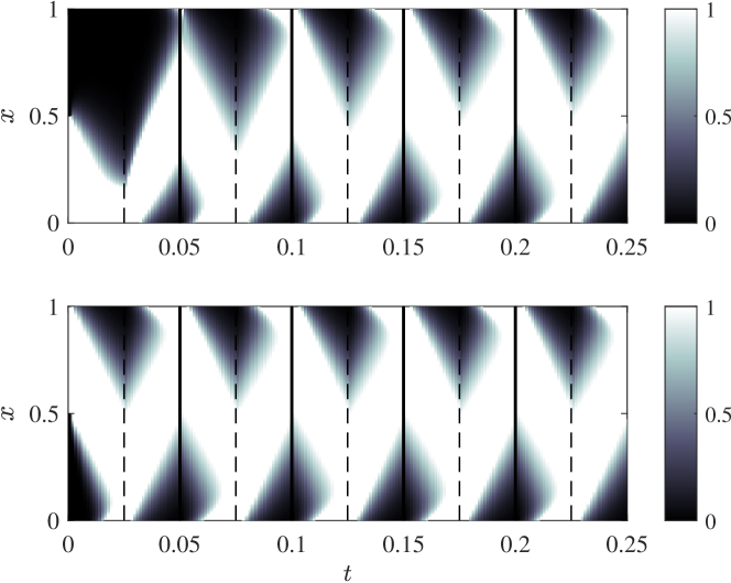
Figure 3: Density $p(x,t)$ for the periodic flow of Section V.2, for two different initial conditions. The two initial conditions converge to the same periodic pattern $\varphi(x,t)$ after about three periods. Here the period $\tau=0.05$ and drift $U=20$, for a domain of width $L=1$ and with diffusivity $D=1$. The vertical lines indicate period boundaries, and the dashed lines are half-periods when the flow switches from right to left.

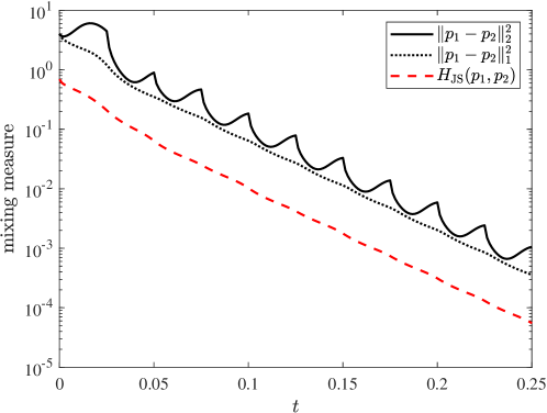
Figure 4: Variance or $L^{2}$ norm (solid line), squared $L^{1}$ norm (dotted line), and Jensen–Shannon divergence (dashed line) between the two solutions in Fig. 3. The variance is nonmonotonic, whereas the $L^{1}$ norm and $H_{\mathrm{JS}}$ decreases monotonically.

In Fig. 3 we show a numerical solution of Eq. V.9, for two different initial conditions: the first ($p_{1}(x,0)$) has particles initially concentrated on the right side of the interval, and the second ($p_{2}(x,0)$) on the left. The two solutions rapidly converge to each other after about three periods. The ultimate state $\varphi(x,t)$ may be considered ‘mixed’ even if it is not uniform. In Fig. 4 we compare the time evolution of variance $\int_{\Omega}\lvert p_{1}-p_{2}\rvert^{2}\mathop{}\!\mathrm{d}{V}$ to the Jensen–Shannon divergence (IV.9). The variance is not at all monotonic: it oscillates about a decreasing trend. The JSD is nice and monotonic, which makes it much easier to assign a numerical value to the decay rate.

V.3 Example of case 2(c): Convergence to an aperiodic density

A simple way to produce an example that is neither steady nor time-periodic is to add some randomness [38]. Recall that in the periodic example of Section V.2 we imposed a flow $U\hat{\bm{x}}$ to the right for a time $\tfrac{1}{2}\tau$, followed by a flow $-U\hat{\bm{x}}$ to the left for a time $\tfrac{1}{2}\tau$, to obtain a period-$\tau$ map. One simple way to randomize this process is to select for every time interval $[t_{k},t_{k}+\tau)$ a uniform independent random number $\alpha_{k}\in[0,1]$, and impose a flow to the right for a time $\alpha_{k}\tau$, followed by a flow to the left for a time $(1-\alpha_{k})\tau$. The kernel Eq. V.10 is then replaced by

$$\mathcal{P}_{\tau,\alpha_{k}}(x\,|\,x_{0})\mathrel{\raisebox{0.29707pt}{:}\!\!=}\int_{0}^{L}P_{-U}(x,(1-\alpha_{k})\tau\,|\,x_{0}^{\prime},0)\,P_{U}(x_{0}^{\prime},\alpha_{k}\tau\,|\,x_{0},0)\,\mathop{}\!\mathrm{d}x_{0}^{\prime}$$ (V.12)

and the map from time $t_{k}$ to $t_{k+1}=t_{k}+\tau$ is

$$p(x,t_{k}+\tau)=\int_{0}^{L}\mathcal{P}_{\tau,\alpha_{k}}(x\,|\,x_{0})\,p(x_{0},t_{k})\mathop{}\!\mathrm{d}x_{0}\,.$$ (V.13)

Figure 5: Density $p(x,t)$ for the random flow of Section V.3, for two different initial conditions. The two initial conditions rapidly converge to the same random pattern $\varphi(x,t)$. The vertical lines indicate period boundaries $t_{k}$, and the dashed lines are the random times $t_{k}+\alpha_{k}\tau$ when the flow switches from right to left. Parameter values are as in Fig. 3.

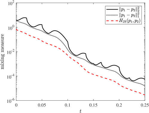
Figure 6: Variance or $L^{2}$ norm (solid line), squared $L^{1}$ norm (dotted line), and Jensen–Shannon divergence (dashed line) between the two solutions in Fig. 5. The variance is nonmonotonic, whereas the $L^{1}$ norm and $H_{\mathrm{JS}}$ decreases monotonically.

In Fig. 5 we show a numerical solution of Eq. V.13, for two different initial conditions, which rapidly converge to each other after about three periods. The ultimate state $\varphi(x,t)$ is ‘mixed’ even though it is neither uniform nor periodic. In Fig. 6 we compare the time evolution of variance $\int_{\Omega}\lvert p_{1}-p_{2}\rvert^{2}\mathop{}\!\mathrm{d}{V}$ to the Jensen–Shannon divergence (IV.9). Much like the periodic case, the variance is not at all monotonic, whereas the JSD relentlessly decreases towards zero.

VI Sources and sinks

VI.1 Varying the number of particles

So far the number of particles was fixed. Now consider the particle density $n(\bm{x},t)\geq 0$ (also sometimes called particle number or number density), which obeys the equation

$$\partial_{t}n+\nabla\cdot\bm{F}(n)=Q(\bm{x},t;n),\qquad\bm{x}\in\Omega,$$ (VI.1)

with the particle flux $\bm{F}(n)=\bm{u}n-\mathbb{D}\cdot\nabla n$ defined as in (II.2). The particle density differs from the probability density $p(\bm{x},t)$ in that the number of particles

$$N(t)=\int_{\Omega}n(\bm{x},t)\mathop{}\!\mathrm{d}{V}$$ (VI.2)

is not necessarily $1$, and can change with time. The number of particles $N(t)$ is not in general an integer. This can either be interpreted as a small error when $N$ is very large, or $n/N$ can be interpreted as a probability.

The source-sink function $Q(\bm{x},t;n)$ is not completely arbitrary: it must preserve the positivity of $n$. There is an asymmetry between adding and removing particles: we can always add particles, but we can only remove particles if there are particles present. One common form of $Q$ that naturally enforces this is

$$Q(\bm{x},t;n)=S(\bm{x},t)-K(\bm{x},t)\,n,\qquad S\geq 0,\ K\geq 0$$ (VI.3)

for given nonnegative functions $S$ and $K$. The source $S$ creates particles indiscriminately, but the sink $-Kn$ vanishes as $n\rightarrow 0$. Of course, more general forms than (VI.3) are possible.

The same considerations for the interior source-sink apply to the flux at the boundary: we should not remove particles if there are none present. Thus, we write for the boundary flux

$$q(\bm{x},t;n)=-\bm{F}(n)\cdot\hat{\bm{n}}=s(\bm{x},t)-k(\bm{x},t)\,n,\qquad s\geq 0,\ k\geq 0,\qquad\bm{x}\in\partial\Omega$$ (VI.4)

for given nonnegative boundary functions $s$ and $k$. The minus sign in front of $\bm{F}\cdot\hat{\bm{n}}$ in (VI.4) is because $\hat{\bm{n}}$ is an outward normal, so $\bm{F}(n)\cdot\hat{\bm{n}}>0$ corresponds to particles leaving the domain $\Omega$.

Using Eqs. VI.2 and VI.1 and the definition of $q$ in (VI.4), we see that the time evolution of $N$ satisfies

$$\dot{}N=\int_{\Omega}Q\mathop{}\!\mathrm{d}{V}+\int_{\partial\Omega}q\mathop{}\!\mathrm{d}{S}$$ (VI.5)

where the first term is the ‘bulk’ source of particles, and the second is the flux of particles across the boundary of $\Omega$.

VI.2 Convergence to asymptotic state

In Section IV we showed that, for one particle (or equivalently a fixed number of noninteracting particles) we can use the $f$-divergence to prove that any two initial conditions will converge to the same ultimate state $\varphi(\bm{x},t)$. The ultimate state may be nonuniform and time-dependent, but what characterizes it is that it is independent of the initial condition: it is an asymptotic state.

Having now allowed for sources and sinks in Section VI.1, we can ask about defining $\varphi(\bm{x},t)$ in that case. After all, adding and removing particles should not prevent two arbitrary initial conditions from converging to each other, as long as they are subjected to the same sources and sinks.

We define the difference $\theta=n_{1}-n_{2}$ between any two solutions of Eq. VI.1. The squared-integral of $\theta$ obeys an equation analogous to the variance evolution Eq. III.4:

$$\frac{\mathrm{d}}{\mathrm{d}{t}}\int_{\Omega}\theta^{2}\mathop{}\!\mathrm{d}{V}=\int_{\Omega}\bm{u}\cdot\nabla\theta^{2}\mathop{}\!\mathrm{d}{V}-2\int_{\Omega}\nabla\theta\cdot\mathbb{D}\cdot\nabla\theta\mathop{}\!\mathrm{d}{V}\\ -2\int_{\Omega}K\,\theta^{2}\mathop{}\!\mathrm{d}{V}-2\int_{\partial\Omega}k\,\theta^{2}\mathop{}\!\mathrm{d}{V}.$$ (VI.6)

The source $S$ does not enter the equation; the last two terms are new but they are nonpositive, so they promote convergence to an equilibrium. However, the same sign-indefinite term involving the integral of $\bm{u}\cdot\nabla\theta^{2}$ appears on the right. This term does go away under the nondivergence and impermeability assumptions (III.1), in which case (VI.6) is enough to conclude convergence to an ultimate state $\varphi(\bm{x},t)$, independent of initial condition.

However, in the divergent or permeable case, we have the same problem as before: the presence of a sign-indefinite term prevents us from guaranteeing convergence. A generalization of the $f$-divergence (IV.2) is needed, with a time evolution that allows us to conclude convergence. We tentatively define

$$H_{f}[n_{1},n_{2}]=\int_{\Omega}n_{2}\,f(n_{1}/n_{2})\mathop{}\!\mathrm{d}{V}.$$ (VI.7)

This is not strictly speaking an $f$-divergence, since $n_{1}$ and $n_{2}$ are not normalized probability densities. The proof from Eq. IV.3 that $H_{f}$ is positive now reads

$$H_{f}[n_{1},n_{2}]=N_{2}\int_{\Omega}f(n_{1}/n_{2})\,p_{2}\mathop{}\!\mathrm{d}{V}\geq N_{2}f\mathopen{}\mathclose{{}\left(\int_{\Omega}(n_{1}/n_{2})\,p_{2}\mathop{}\!\mathrm{d}{V}}\right)=N_{2}f(N_{1}/N_{2})$$

where $N_{i}=\int_{\Omega}n_{i}\mathop{}\!\mathrm{d}{V}$, and $p_{i}=n_{i}/N_{i}$ are normalized probability densities. Hence, to guarantee $H_{f}[n_{1},n_{2}]\geq 0$ we must add the additional requirement that $f\geq 0$, which is satisfied by the Jensen–Shannon choice (IV.8) for $f$. (To satisfy $f\geq 0$, the Kullback–Leibler choice (IV.5) can simply be modified to read $f(u)=u\log u-u+1$, in which case $H_{f}$ is sometimes called the physical relative entropy.) With this additional constraint on $f$, we have $H_{f}[n_{1},n_{2}]=0$ if and only if $n_{1}\equiv n_{2}$.

With the same approach as in Appendix A we can show that the time evolution of $H_{f}[n_{1},n_{2}]$ is given by

$${\dot{H_{f}\mkern-3.0mu}\mkern 3.0mu}{}[n_{1},n_{2}]=-\int_{\Omega}n_{2}\,f^{\prime\prime}(n_{1}/n_{2})\,\nabla(n_{1}/n_{2})\cdot\mathbb{D}\cdot\nabla(n_{1}/n_{2})\mathop{}\!\mathrm{d}{V}\\ -\int_{\Omega}\mathopen{}\mathclose{{}\left(Kn_{2}f(n_{1}/n_{2})+S\,g_{f}(n_{1}/n_{2})}\right)\mathop{}\!\mathrm{d}{V}\\ -\int_{\partial\Omega}\mathopen{}\mathclose{{}\left(kn_{2}f(n_{1}/n_{2})+s\,g_{f}(n_{1}/n_{2})}\right)\mathop{}\!\mathrm{d}{S}\leq 0,$$ (VI.8)

where

$$g_{f}(u)\mathrel{\raisebox{0.29707pt}{:}\!\!=}(u-1)f^{\prime}(u)-f(u)\geq 0,\qquad g_{f}(1)=0.$$ (VI.9)

The inequality in (VI.8) follows from the positivity of $n_{i}$, the strict convexity of $f$ ($f^{\prime\prime}>0$), the positive-definiteness of $\mathbb{D}$, the nonnegativity of $f$, $K$, $S$, $k$, $s$, and the inequality in (VI.9). (The latter is easy to prove: a differentiable convex function satisfies $f(x)\geq f(y)+(x-y)f^{\prime}(y)$ for all $x$, $y$, since its graph is above all its tangents; set $x=1$ and $y=u$ and use $f(1)=0$.) The right-hand side of (VI.8) vanishes if and only if $n_{1}=n_{2}$.

VII Total variation distance and $L^{1}$ norm

As an alternative to the $f$-divergence, another measure of convergence of two densities is the total variation distance (or variational distance), which is equivalent to $\tfrac{1}{2}\lVert p_{1}-p_{2}\rVert_{1}$ [36], where $\lVert\cdot\rVert_{1}$ is the $L^{1}$ norm on $\Omega$. Compare the evolution of $\lVert p_{1}-p_{2}\rVert_{1}^{2}$ to the concentration variance $\lVert p_{1}-p_{2}\rVert_{2}^{2}$ in Figs. 4 and 6. Notice that the $L^{1}$ norm, much like $H_{f}$, decays monotonically, exhibiting none of the troublesome oscillations of the $L^{2}$ norm (variance). In this section we will show that the $L^{1}$ norm does indeed always decrease monotonically, so that it is a more reliable measure of mixing than the $L^{2}$ norm for nonuniform mixing.

We shall prove this for two general number densities $n_{1}$ and $n_{2}$ obeying Eq. VI.1 with the source-sink (VI.3), and with boundary conditions (VI.4). Let $\theta=n_{1}-n_{2}$, which satisfies $\partial_{t}\theta=-\nabla\cdot\bm{F}(\theta)-K\theta$ and $\bm{F}(\theta)\cdot\hat{\bm{n}}=k\,\theta$ on $\partial\Omega$. For any function $G(\theta)$, we have

$$\frac{\mathrm{d}}{\mathrm{d}{t}}\int_{\Omega}G(\theta)\mathop{}\!\mathrm{d}{V}=\int_{\Omega}G^{\prime\prime}(\theta)\,\theta\bm{u}\cdot\nabla\theta\mathop{}\!\mathrm{d}{V}-\int_{\Omega}G^{\prime\prime}(\theta)\,\nabla\theta\cdot\mathbb{D}\cdot\nabla\theta\mathop{}\!\mathrm{d}{V}\\ -\int_{\Omega}G^{\prime}(\theta)\,K\theta\mathop{}\!\mathrm{d}{V}-\int_{\partial\Omega}G^{\prime}(\theta)\,k\theta\mathop{}\!\mathrm{d}{S}$$ (VII.1)

which is a generalization of Eq. VI.6. Now let $G(\theta)=\lvert\theta\rvert$, so that $G^{\prime}(\theta)=\operatorname{sgn}(\theta)$ and $G^{\prime\prime}(\theta)=2\delta(\theta)$. With that choice, Eq. VII.1 becomes

$$\frac{\mathrm{d}}{\mathrm{d}{t}}\lVert\theta\rVert_{1}=2\int_{\Omega}\delta(\theta)\,\theta\bm{u}\cdot\nabla\theta\mathop{}\!\mathrm{d}{V}-2\int_{\Omega}\delta(\theta)\,\nabla\theta\cdot\mathbb{D}\cdot\nabla\theta\mathop{}\!\mathrm{d}{V}-\int_{\Omega}K\lvert\theta\rvert\mathop{}\!\mathrm{d}{V}-\int_{\partial\Omega}k\lvert\theta\rvert\mathop{}\!\mathrm{d}{S}.$$

The first term on the right vanishes since the delta function forces $\theta=0$; for the second term, we can turn the volume integral into a surface integral [39, Theorem 6.1.5]:

$$\frac{\mathrm{d}}{\mathrm{d}{t}}\lVert\theta\rVert_{1} =-2\int_{\{\theta=0\}}\nabla\theta\cdot\mathbb{D}\cdot\nabla\theta\,\frac{\mathop{}\!\mathrm{d}{S}}{\lvert\nabla\theta\rvert}-\int_{\Omega}K\lvert\theta\rvert\mathop{}\!\mathrm{d}{V}-\int_{\partial\Omega}k\lvert\theta\rvert\mathop{}\!\mathrm{d}{S}\leq 0,$$ (VII.2)

where the first integral is over the zero level set of $\theta(\cdot,t)$. We conclude that the total variation distance $\tfrac{1}{2}\lVert n_{1}-n_{2}\rVert_{1}$ does indeed decrease monotonically, as was apparent from the earlier numerical simulations. (The level-set integral in Eq. VII.2 appears in approaches based on tracer coordinates [40].)

The ‘proof’ presented here relies on the apparently strong assumption that $\lvert\nabla\theta\rvert\neq 0$ on the zero level set of $\theta$. However, the uniform ellipticity bound (III.5) implies that $-\nabla\theta\cdot\mathbb{D}\cdot\nabla\theta/\lvert\nabla\theta\rvert\leq-\sigma\lvert\nabla\theta\rvert$, so singular points limit nicely to zero in the integrand. In Appendix B we show that the $L^{1}$ norm is the only $L^{q}$ norm that decays monotonically in the nonuniform mixing case.

One possible advantage Eq. VII.2 has over the corresponding equation (VI.8) for the $f$-divergence is that it shows convergence even when the source $S(\bm{x},t)$ is negative, since the source has dropped out of (VII.2) completely. However Eq. VI.8 suggests that a positive source can actually improve the rate of convergence. Another weakness of Eq. VII.2 compared to (VI.8) is that the its right-hand side is difficult to compute: it requires tracking of the zero level set, which is a challenging problem in practice because of resolution and changes in topology. By comparison, the right-hand side of Eq. VI.8 is readily computed and regions of large entropy production can be identified from the magnitude of the integrands.

VIII Discussion

The traditional view of mixing in nondivergent flow is that a stirred passive scalar will ultimately be homogenized to a uniform concentration. As we discussed, this requires both nondivergence of the velocity field and no-penetration boundary conditions. If either condition is violated, the ultimate state of the mixing process is no longer uniform, and may in fact be time-dependent for nonautonomous systems, where $\bm{u}$ or $\mathbb{D}$ are explicit functions of time. We refer to these systems as nonuniform mixing, because the passive scalar may be mixed even though its concentration is not uniform. Such nonuniform situations will arise in the presence of filters, which are membranes that permits the passage of fluid but not of particles (passive scalar).

Using the standard concentration variance as a proxy for mixing is less useful for nonuniform mixing, since the variance is not necessarily a monotonically-decreasing function of time. Of course, variance will eventually decrease to zero even in nonuniform mixing (as long as it it defined appropriately), but the excursions it undertakes can make it hard to ascribe a rate of mixing to the system (see Figs. 4 and 6). Instead of concentration variance, a more reliable proxy for mixing is the $f$-divergence, which is related to relative entropy. Instead of relying an initial condition to become uniform, we define the rate of mixing in terms of the rate at which two arbitrary densities $p_{1}(\bm{x},t)$ and $p_{2}(\bm{x},t)$ approach each other. They will eventually both converge to an ultimate density $\varphi(\bm{x},t)$, which is independent of the initial condition. The $f$-divergence picture is easily adapted to cases with sources and sinks.

The connection between the $f$-divergence and mix-norms [41, 42, 4] is not completely clear. Mix-norms are used as a diagnostic for mixing, and are not guaranteed to decay monotonically for the types of examples presented here. Their behavior is thus probably more closely related to that of concentration variance than to $f$-divergence, though they have the advantage that they decay even when the diffusivity is set to zero, which renders them more useful for optimization [43, 44, 45, 46, 47]. Perhaps there is a hybrid approach that could marry the advantages of both.

Finally, note that nonuniform mixing suggests a different type of mixing optimization problem, where the goal is to decrease spatial or temporal variations of $\varphi(\bm{x},t)$ itself rather than the rate of approach to $\varphi(\bm{x},t)$. This was investigated previously for source-sink systems [48, 49, 50, 51], but it could be effected in any problem involving nonuniform mixing. For example, a flow could be designed to minimize the concentration of viruses near a filter, to mitigate the effect of inevitable imperfections in the membrane.

Appendix A Derivation of Eq. IV.4

Write $\partial_{t}p_{i}=-\nabla\cdot\bm{F}(p_{i})$, with $\bm{F}(p)\mathrel{\raisebox{0.29707pt}{:}\!\!=}\bm{u}\,p-\mathbb{D}\cdot\nabla p$, and consider a domain $\Omega\subset\mathbb{R}^{n}$ with $\bm{F}(p_{i})\cdot\hat{\bm{n}}=0$ on $\partial\Omega$. Then by direct differentiation of Eq. IV.2:

$${\dot{H_{f}\mkern-3.0mu}\mkern 3.0mu}{}[p_{1},p_{2}] =\int_{\Omega}\mathopen{}\mathclose{{}\left(\partial_{t}p_{2}\,f(p_{1}/p_{2})+p_{2}\,f^{\prime}(p_{1}/p_{2})\mathopen{}\mathclose{{}\left(\partial_{t}p_{1}/p_{2}-p_{1}\,\partial_{t}p_{2}/p_{2}^{2}}\right)}\right)\mathop{}\!\mathrm{d}{V}$$

$$=-\int_{\Omega}\mathopen{}\mathclose{{}\left(\nabla\cdot\bm{F}(p_{2})\,f(p_{1}/p_{2})+f^{\prime}(p_{1}/p_{2})\mathopen{}\mathclose{{}\left(\nabla\cdot\bm{F}(p_{1})-(p_{1}/p_{2})\nabla\cdot\bm{F}(p_{2})}\right)}\right)\mathop{}\!\mathrm{d}{V}.$$

We integrate by parts, and two terms containing $f^{\prime}(p_{1}/p_{2})\,\bm{F}(p_{2})\cdot\nabla(p_{1}/p_{2})$ cancel. We are left with

$$\dot{}H_{f}[p_{1},p_{2}]=\text{BT}[p_{1},p_{2}]+\int_{\Omega}p_{2}^{-1}f^{\prime\prime}(p_{1}/p_{2})\nabla(p_{1}/p_{2})\cdot\mathopen{}\mathclose{{}\left(p_{2}\bm{F}(p_{1})-p_{1}\bm{F}(p_{2})}\right)\mathop{}\!\mathrm{d}{V}$$ (A.1)

with the boundary terms

$$\text{BT}[p_{1},p_{2}] =-\int_{\partial\Omega}f(p_{1}/p_{2})\,\bm{F}(p_{2})\cdot\hat{\bm{n}}+p_{2}^{-1}\,f^{\prime}(p_{1}/p_{2})\mathopen{}\mathclose{{}\left(p_{2}\bm{F}(p_{1})-p_{1}\bm{F}(p_{2})}\right)\cdot\mathop{}\!\mathrm{d}{\bm{S}}.$$

The boundary terms vanish when $\bm{F}(p_{i})\cdot\hat{\bm{n}}=0$ on $\partial\Omega$. Also,

$$p_{2}\bm{F}(p_{1})-p_{1}\bm{F}(p_{2}) =p_{2}(\bm{u}\,p_{1}-\mathbb{D}\cdot\nabla p_{1})-p_{1}(\bm{u}\,p_{2}-\mathbb{D}\cdot\nabla p_{2})$$

$$=-p_{2}\mathbb{D}\cdot\nabla p_{1}+p_{1}\mathbb{D}\cdot\nabla p_{2}$$

$$=-p_{2}^{2}\,\mathbb{D}\cdot\nabla(p_{1}/p_{2}).$$ (A.2)

Inserting (A.2) into (A.1) recovers Eq. IV.4.

Appendix B Decay of $L^{q}$ norms

For $1\leq q\leq\infty$, does any $L^{q}$ norm other than $q=1$ decay monotonically? If we put $G(\theta)=\lvert\theta\rvert^{q}$ in Eq. VII.1, then for $q$ even we have $G(\theta)=\theta^{q}$, $G^{\prime}(\theta)=q\theta^{q-1}$, and $G^{\prime\prime}(\theta)=q(q-1)\theta^{q-2}$, and find

$$\frac{\mathrm{d}}{\mathrm{d}{t}}\lVert\theta\rVert_{q}^{q}=q(q-1)\int_{\Omega}\theta^{q-1}\,\bm{u}\cdot\nabla\theta\mathop{}\!\mathrm{d}{V}-q(q-1)\int_{\Omega}\theta^{q-2}\,\nabla\theta\cdot\mathbb{D}\cdot\nabla\theta\mathop{}\!\mathrm{d}{V}$$ (B.1)

where we set $K=k=0$ for convenience. The first term on the right is not sign definite for any even $q$, so none of these norms will necessarily decay monotonically. For $q$ odd, we have that $G^{\prime}(\theta)=q\theta^{q-1}\operatorname{sgn}(\theta)$ and $G^{\prime\prime}(\theta)=2q\theta^{q-1}\delta(\theta)+q(q-1)\theta^{q-2}\operatorname{sgn}(\theta)$, and Eq. VII.1 becomes

$$\frac{\mathrm{d}}{\mathrm{d}{t}}\lVert\theta\rVert_{q}^{q}=q(q-1)\int_{\Omega}\theta^{q-2}\lvert\theta\rvert\,\bm{u}\cdot\nabla\theta\mathop{}\!\mathrm{d}{V}\\ -2q\int_{\Omega}\theta^{q-1}\delta(\theta)\,\nabla\theta\cdot\mathbb{D}\cdot\nabla\theta\mathop{}\!\mathrm{d}{V}-q(q-1)\int_{\Omega}\lvert\theta\rvert^{q-2}\,\nabla\theta\cdot\mathbb{D}\cdot\nabla\theta\mathop{}\!\mathrm{d}{V}.$$ (B.2)

For $q=1$ this reduces to Eq. VII.2; for $q>1$ we have

$$\frac{\mathrm{d}}{\mathrm{d}{t}}\lVert\theta\rVert_{q}^{q}=q(q-1)\int_{\Omega}\theta^{q-2}\lvert\theta\rvert\,\bm{u}\cdot\nabla\theta\mathop{}\!\mathrm{d}{V}-q(q-1)\int_{\Omega}\lvert\theta\rvert^{q-2}\,\nabla\theta\cdot\mathbb{D}\cdot\nabla\theta\mathop{}\!\mathrm{d}{V}.$$ (B.3)

and again the first term is not sign-definite. We conclude that the $L^{1}$ norm is the only such norm that exhibits a monotonic decay to zero in the nonuniform mixing case.